Quantifying the Callable Risk of a Bond Portfolio A Binomial Approach

Bert Korevaar & Gert Verheij

AMRO Bank / FMG Investment Research, Rallypost 422, PO Box 283, 1000 EA Amsterdam, The Netherlands

Summary

This article deals with pricing in the Dutch Private Loan Market in general and the valuation of callable bonds in this market in particular. This subject is gaining importance now that portfolio management is placing increasing emphasis on risk management rather than on the maximisation of effective returns. Furthermore, it is expected that borrowers will in the future make increasing use of their right to call bonds before maturity.

The Dutch Private Loan Market is characterised by a wide diversity of loan modalities in combination with a secondary market that lacks liquidity. The valuation model described in this article is based on the term structure of the Dutch Public Bond Market.

A callable bond can only be valued accurately if we take account of the option component of the bond. The right to call the bond before maturity, after all, is basically a call option written by the investor who receives a premium from the issuer in return. Due to the hybrid nature of options (both European and American) and their variable exercise prices, options cannot be effectively analysed with the Black & Scholes option valuation model. The binomial model offers a more practicable approach.

The option theory enables us to derive the duration and convexity of callable bonds. A significant factor is that the convexity may become negative when the option is in the money, i.e. when the issuer stands to gain from exercising the right to call before maturity.

The derived model makes it possible to include in a proper way callable bonds in any portfolio analysis and/or performance system. Alternative approaches based on the duration till maturity or till the first callable date will result in an inaccurate analysis of the risk involved in the fixed-interest portfolio.

329

Résumé

Quantifier le Risque Remboursable d'un Portefeuille d'Obligations Une Approche Binomiale

Cet article traite de la tarification dans le Marché des Prêts Privés hollandais en général et de l'évaluation des obligations remboursables dans ce marché en particulier. Ce sujet est de plus en plus important maintenant que la gestion de portefeuille se concentre de plus en plus sur la gestion du risque plutôt que sur la maximisation des rendements effectifs. De plus, on s'attend à ce que les emprunteurs utilisent de plus en plus, à l'avenir, leur droit d'amortir les obligations avant l'échéance.

Le Marché des Prêts Privés hollandais se caractérise par une grande diversité de modalités de prêts alliée à un marché secondaire qui manque de liquidité. Le modèle d'évaluation décrit dans cet article est basé sur la structure d'échéance du Marché des Obligations Publiques hollandais.

Une obligation remboursable ne peut être évaluée avec exactitude que si nous tenons compte du composant optionel de l'obligation. Après tout, le droit d'amortir l’obligation avant l'échéance est en fait une option d'achat souscrite par l'investisseur qui reçoit en échange une prime de l’émetteur. Etant donnée la nature hybride des options (à la fois européennes et américaines) et leur prix de levée variable, les options ne peuvent pas être efficacement analysées avec le modèle d'évaluation d'options Black & Scholes. Le modèle binomial offre une approche plus facile à utiliser.

La théorie des options nous permet de decluire la durée et la convexité des obligations remboursables. Un facteur important est que la convexité peut devenir négative lorsque l'option est dans l’argent, c'est-à-dire quand l'assureur a des chances de faire un gain en exerçant le droit d'amortissement avant échéance.

Le modèle dérivé permet d'inclure d'une façon appropriée des obligations remboursables dans toute analyse de portefeuille et/ou système de performance. D'autres approches basées sur la durée jusqu'à l'échéance ou jusqu'à la première date d'amortissement anticipé conduiront à une analyse inexacte du risque impliqué dans le portefeuille à intérêt fixe.

330

1 Introduction

1.1 Dutch institutional investors

Institutional investors (insurance companies and pension funds) traditionally make up the largest

market party on the supply side of the Dutch capital market. The tremendous flight of collective

saving in the past decades has resulted in a sharp increase in their investable funds, now

totalling approximately 120% of the Dutch gross national product.

Dutch institutional investors, as a rule, pursue a cautious, risk-averse investment policy. In the

Dutch situation this is natural as their obligations consist mainly of long-term guilder

commitments. The composition of their investment portfolios - particularly the sizable fixed-

interest component - illustrates the point.

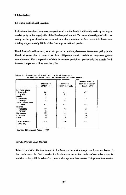
Table 1: Portfolios of Dutch institutional investors (at end September 1989, as percentage of total assets)

Private loans - Domestic - Foreign Bonds - Domestic - Foreign Total bonds and

Loans

Shares - Domestic - Foreign Mortgages Property Cash

Total assets (Dfl bn)

Insurance Private Companies Pension Funds

46 2

7 2

57

41 2

15 5

63

10 3

22 8 0

142 219

Source: DNB Annual Report 1989

1.2 The Private Loan Market

8 11 4

11 3

General Public Service Pension

Fund (ABP)

69 1

13 1

84

3

1 6 0

151

Table 1 subdivides the investments in fixed-interest securities into private loans and bonds. It

does so because the Dutch market for fixed-interest securities consists of two submarkets. In

addition to the public bond market, there is also a private loan market. This private loan market

331

1

is unique in the world of international finance. The difference between bonds and private loans

is that the former are aimed at the investing public at large while the latter are targeted at a

single or limited number of investor(s). With private loans, the borrower and lender lay down

their mutual obligations regarding payments and payment dates in a written agreement.

The private loan market, no doubt, offers Dutch institutional investors certain advantages. The

main advantages of private loans over ordinary bonds are:

- The conditions of the loan can easily be adapted to the requirements of borrowers and

lenders;

- Issues involve no more than a few participants;

- Issues can be made at any time;

- The lender has the advantage of the higher interest rate paid on private loans;

- The borrower’s costs are lower (no prospectus, no publicity, lower fees).

However portfolio managers are now also waking up to its drawbacks. Two of these are

discussed in this article. The first concerns low liquidity and non-transparent pricing in the

private loan market. The second has to do with the built-in right to call before maturity, which

is an extremely frequent phenomenon in the private loan market. Though the maturity of loans

is longer in the private loan market than in the public bond market, virtually all private loans

with terms over ten years are callable. The conditions - e.g. the penalty percentages - are often

laid down in standard contracts.

What then persuaded investors in the past to turn to the private loan market in spite of the

disadvantages? It could be that investors were prepared to accept these disadvantages provided

the private loan market offered sufficiently higher returns than the public market. The low

liquidity of the private loan market did not concern them as the private loans were seen as a

core holding in the total investment portfolio. Their willingness to accept callable bonds also

derives from the desire to maximise effective returns, which was once the prime objective of

portfolio managers. Bonds called before maturity, after all, yield higher returns than non-

callable bonds. But today the private loan market is beginning to lose ground. This has partly

to do with a shift in portfolio management priorities. No longer is the maximisation of effective

returns the sole concern. Portfolio managers are gearing their strategies increasingly to

maturities policy (i.e. riskmanagement). To achieve this, portfolios must satisfy liquidity

requirements. Portfolio managers also want the flexibility to pursue an active investment strategy

within the framework of the overall investment policy. Another reason for the dwindling interest

in the private loan market may therefore be that the maturity of callable bonds is unpredictable,

making them unsuitable for an active, optimising policy.

332

In addition, callable bonds also have a remarkable effect on the performance of fixed-interest

portfolios. For, in practice, performance measurement systems treat such bonds as short

maturities when the current interest rate is significantly lower than the coupon of the loan. This

is natural as it is realistic to assume that in such cases the bonds will be redeemed at the

earliest opportunity (next callable date). But suppose interest rates rise again, then the interest

gap will narrow and so automatically extend the maturity of the bonds. This is an odd twist.

After all, when interest rates rise it is better to have your funds invested in short-term loans.

The same applies in the case of falling interest rates. It is needless to point out the disastrous

effects on the overall performance of the portfolio.

Due to these disturbing developments, there is a growing need to find an effective method for

pricing private loans in general and callable private loans in particular. This need has become

even more acute following a recent official announcement stating that the Dutch government,

one of the largest borrowers in the private loan market, intends in the coming years to make

frequent use of its right to call before maturity. The 1989 annual report on the national debt 1

puts it as follows: “In 1989 the Agency called a large number of private loans totalling NLG

725m before maturity. The number of loans eligible for early redemption will increase

significantly in the coming years. The redemption of these loans will depend on interest rate

movements.” There can be little doubt that other major borrowers will follow suit.

In conjunction with one of the largest pension funds in the Netherlands , a model has been 2

developed to allow the valuation of private loans. Particular attention has been devoted to

callable private loans. Drawing on the existing literature , this article tries to combine the 3

various aspects involved in order to arrive at a consistent method for including callable private

loans in portfolio analysis and/or performance systems. Section 2 first introduces the reader to

the pricing mechanism in the private loan market and then describes the valuation model.

Section 3 gives the derivations of certain yardsticks for determining the interest sensitivity of

callable bonds. Section 4 illustrates the theory with an example. Finally some conclusions are

given in section 5.

1 Agency of Finance, 1989

2 Unilever Pension Fund “Progress”, Rotterdam

3 In particular, De Munnik & Vorst, 1989 and Dunetz & Mahoney, 1988

333

2 Pricing and valuation

2.1 Pricing in the private loan market

Pricing private loans forms a problem for borrowers and lenders alike because there is no frame

of reference. The first snag is the extremely diverse nature of the loans themselves. Basically

each loan is unique. The second problem is the low liquidity of the secondary market. In the

primary market, the borrower contacts the lender through a intermediary and negotiations are

held to determine the modalities and price of the loan. Mostly the public bond market serves

as a frame of reference for these negotiations. The interest rates applicable to similar bonds in

the public bond market are used to determine the yield spread. Research shows that the longer 4

the life of the loan is, the higher the yield spread will be, and that in the past the spreads of

longer-term loans fluctuated less than those of shorter-term loans.

Figure 1: Yield spread between Public Bond Market and Private Loan Market

Source: AMRO Bank

4 AMRO Bank, 1989

334

From 1985 to 1989, the difference between the yield spread on private loans and public bonds

ranged overall from -25 to 50 basis points (see figure 1). The average spread for short-term

government loans, for instance, was 12 basis points with a variance of 16 basis points, while the

average for long-term government loans was 17 basis points with a variance of 10 basis points.

The public bond market, in our view, also offers a good point of reference for pricing loans

in the secondary private loan market. This article is based on the term structure of government

bonds in the public market. By estimating the spreads available between the public and private

market, it is possible to derive the term structure of the private loan market.

2.2 The Pricing of Callable Bonds

Pricing callable bonds is a complicated business both in the public and private markets. There

are relatively few capable bonds listed in the Dutch public bond market so this does not really

present a problem in the Netherlands. In the private loan market, however, callable bonds are

quite common. In this already highly non-transparent market, it is important to be able to price

callable bonds accurately.

Practitioners often overvalue callable bonds, simply because they tend to underestimate the role

of the option component. We should bear in mind that a callable bond is basically a bond with

a written call option. The issuer has bought the right from the investor to call the bond before

the normal redemption date. In return for this right the investor receives a premium. The

underestimation of the option component becomes apparent when we look at the way in which

callable bonds are valued in practice. Callable bonds are usually valued on the basis of maturity

till normal redemption or on the basis of the maturity until the earliest callable date. The

minimum of the resulting two prices determines the ultimate price. This price only indicates

the upper limit of the callable bond’s value. As a result, the callable bond is often overvalued.

Specific option valuation techniques provide a more fruitful way of setting the price of callable

bonds. Only recent literature devotes attention to these techniques and so far they have not

received widespread application in practice. The best-known option valuation method - the

Black & Scholes method - is not very useful as most callable bonds are not purely European

options, but rather options with a combination of European and American characteristics. They

are European in that the issuer is not allowed to redeem the bond before a specified date, but

American in that after this specified date they can be redeemed at any time (in the case of

Dutch government bonds) or on any future coupon date (in the case of other borrowers).

335

Another reason why the Black & Scholes model is not suitable is that different penalty

percentages apply depending on the different callable dates. The Black & Scholes model is

unable to take account of these variable exercise prices.

The binomial model (from which the Black & Scholes model can be derived) offers us an

alternative approach. The problems mentioned above do not occur in using the binomial model.

This model involves the construction of a tree of possible underlying values. The theoretical

value of the option can then be calculated on the basis of the tree and the various characteristics

of the option.

23 Valuation model for callable bonds 5

In this section we give a description of the binomial valuation model. First a distribution of

forward rates will be derived. Secondly, we use this distribution to build up a tree of possible

forward rates. As an example we apply this tree to a so-called tow-period model. After that this

principle can be expanded to an n-period model. On the basis of this n-period model of a

forward rate tree and the cashflow scheme of a bond, the price of the bond can be calculated.

We then describe a specific feature of the model in the valuation of callable bonds.

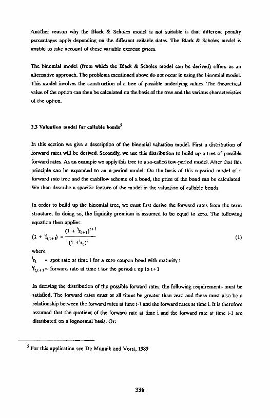
In order to build up the binomial tree, we must first derive the forward rates from the term

structure. In doing so, the liquidity premium is assumed to be equal to zero. The following

equation then applies:

where

= spot rate at time i for a zero coupon bond with maturity t

= forward rate at time i for the period t up to t + 1

(1)

In deriving the distribution of the possible forward rates, the following requirements must be

satisfied. The forward rates must at all times be greater than zero and there must also be a

relationship between the forward rates at time i-1 and the forward rates at time i. It is therefore

assumed that the quotient of the forward rate at time i and the forward rate at time i-1 are

distributed on a lognormal basis. Or:

5 For this application see De Munnik and Vorst, 1989

336

Another reason why the Black & Scholes model is not suitable is that different penalty

percentages apply depending on the different callable dates. The Black & Scholes model is

unable to take account of these variable exercise prices.

The binomial model (from which the Black & Scholes model can be derived) offers us an

alternative approach. The problems mentioned above do not occur in using the binomial model.

This model involves the construction of a tree of possible underlying values. The theoretical

value of the option can then be calculated on the basis of the tree and the various characteristics

of the option.

23 Valuation model for callable bonds 5

In this section we give a description of the binomial valuation model. First a distribution of

forward rates will be derived. Secondly, we use this distribution to build up a tree of possible

forward rates. As an example we apply this tree to a so-called tow-period model. After that this

principle can be expanded to an n-period model. On the basis of this n-period model of a

forward rate tree and the cashflow scheme of a bond, the price of the bond can be calculated.

We then describe a specific feature of the model in the valuation of callable bonds.

In order to build up the binomial tree, we must first derive the forward rates from the term

structure. In doing so, the liquidity premium is assumed to be equal to zero. The following

equation then applies:

where

= spot rate at time i for a zero coupon bond with maturity t

= forward rate at time i for the period t up to t+1

(1)

In deriving the distribution of the possible forward rates, the following requirements must be

satisfied. The forward rates must at all times be greater than zero and there must also be a

relationship between the forward rates at time i-1 and the forward rates at time i. It is therefore

assumed that the quotient of the forward rate at time i and the forward rate at time i-1 are

distributed on a lognormal basis. Or:

5 For this application see De Munnik and Vorst, 1989

337

(2)

Suppose n=2, i.e. that two periods remain before the expiration of the callable date of the

bond. The binomial tree can then be constructed as follows:

where

= the first possible forward rate over period 1 to 2

= the second possible forward rate over period 1 to 2

Suppose also that the chance of forward rate f 1 12 occurring in period 1 is equal to the chance

of forward rate f 2 1,2 occurring in period 1. On the basis of this assumption and the distribution

assumed earlier (see equation (2)), the following equation can be derived:

The following can be derived for the standard deviation:

It then follows from equation (4) that:

(3)

(4)

(5)

As discounting must take place in the binomial tree according to the discount rate applicable

to the current term structure, equations (1), (3) and (5) permit the derivation of the following

equations:

(6)

where

= the spot rate at time i

= the standard deviation of the forward rate over period 1 to 2

338

As the term structure - and hence the spot rates r 1 and r 2 are known while the standard

deviation is also known - it is possible to derive f from equation (6). We make use of σ 1,2 1 1,2

the term structure of the Dutch government bonds in the public market and a predetermined

spread between this market and the private loan market to get the spot rates. In addition,

historical data are used to determine the volatility of the term structure. The model makes use

of the standard deviations of spot rates and forward rates which are estimated on the basis of

a 10-year history of monthly term structures. f from equation (6) can be derived by means 1 1,2

of the Secanten Method Equation (5) then results in f . 6 2

1,2

This principle can then be. expanded by assuming that there are n periods - instead of two

periods - remaining before the redemption date of the callable bond. This results in the

following binomial tree:

The following equations apply to this tree:

(7)

(8)

As r and r are already known on the basis of the term structure and as the standard t t+1

deviation σ is predetermined, equation (7) allows us to calculate the value for f while t,t+1

1 t,t+1

equation (8) permits the calculation of values f up to and including f . 2 t+1

t,t+1 t,t+1

6 Cheney and Kincaid, 1985

339

The binomial tree of forward rates makes it possible to calculate the price of any bond by

means of a recursive process. We know that the bond is redeemed at 100% and the final

coupon is received on the maturity date. The value of this can be determined, one period before

the maturity date, with the aid of the forward rates f the expected interest for the period i n-1,n ,

n-1 to n. This results in n different values.

for i = 1..n-1 (9)

where

C = the price of the bond n-1 periods after today i n-1

For one period further back, we can determine the values using the forward rates f , the i n-2,n-1

expected interest for the period n-2 to n-1. These values are determined by means of the

following equation.

where

C i t = the price of the bond t periods after today

for i = 1..n-1 and t = 1..n-1 (10)

By repeating this process, a binomial tree of bond prices is built up, eventually permitting us

to determine the value C , i.e. the value of the bond at the present instant. 0

1

We can apply this principle in order to determine the present value of a callable bond, Cb . For 0

every callable period before maturity (i.e. in every knot of the binomial tree), the issuer will

weigh up the pros and cons of early redemption. If the early redemption value plus the coupon

(or current coupon) exceeds the value of the callable bond in the relevant knot, the bond will

340

not be called before maturity. But if it is lower, the bond will be redeemed before maturity and

the value in the knot will be replaced with the early redemption value plus the coupon, equal

to ER . The resulting binomial tree is built up with the aid of the following equations: t

for i = 1...n

for i = 1...n

(11)

(12)

for i = 1...t+1 and t = 1...n-2 (13)

(14)

if early redemption is possible at time i

other

for t = 0..n-1 (15)

In this way it is possible to determine the value of every callable bond. The value of the option

can be calculated as follows. Calculate the value of the underlying bond without the option

feature be equation (8) to (9). The difference between the value of the callable bond and the

value of the underlying bond is the value of the option.

So far we have been silent about the number and length of the periods. In the equations above,

it was assumed that the periods coincided with the coupon date of the bond. So we assumed

that issuers only considered the call option on the coupon dates. In the developed model, we

opted for the following time division. Period 1 is the time between today and the next coupon

date. The other periods run from the coupon date to the next coupon date. This choice does

mean that we need to take current interest into account in the first period. The value of the

callable bond therefore is Cb , including current interest (for which an adjustment must be 0

made). The model can be adjusted to situations where the issuer does not only consider coupon

dates in excersising his option. In such a situation we need to take current interest into account

at every time.

The model also assumes that the issuer always acts as a rational decision-maker. In practice,

however, a relative attractive level of interest rates certainly do not always lead to early

341

redemption. Issuers may be reluctant to call for various reasons, such as refinancing costs, the

simultaneous callability of several bonds, balance sheet or budgetary considerations, and so on.

It turns out that issuers considering early redemption often take account of a higher penalty

percentage than they will actually be required to pay. On the basis of past experience, it is

possible to take account of this fictitious interest percentage in the model.

The above equations all assume that the bond is repaid at the end of the period of the bond.

Though this is becoming an increasingly common practice in the Netherlands both in the public

and private markets, the issuance of such bullet bonds was not permitted in the Netherlands

until the beginning of 1986. Before 1986 borrowers were obliged to repay the bond in at least

four equal annual installments. Many of the currently outstanding bonds, particularly in the

private market, date from before 1986 and therefore cannot be redeemed in one amount. This

aspect must be taken into account in the binomial tree7.

3. Interest Sensitivity

3.1 Duration and Convexity

In the past 20 years duration of bonds has developed into an important tool for portfolio

managers of fixed-interest securities. The duration gives a fairly accurate idea as to how

sensitive the bond is to interest rate fluctuations and is widely used as a yardstick for measuring

the interest rate risk involved in bond portfolios. The interest in convexity is of more recent

date. Convexity allows us to trace the relationship between the bond price and the current

interest rate and so improves our insight into the interest sensitivity of bonds, particularly when

interest rates are volatile. Positive convexity implies that the bond price will rise faster when

interest rates fall than it will drop when interest rates rise (see figure 2).

Most research in this field has so far concentrated on non-callable bonds. In such cases, the

duration and the convexity is relatively easy to determine as the cashflows are known and fixed.

But callable bonds are a different matter; both the maturity and volume of the cashflows are

uncertain. This means that neither the duration nor the convexity can be calculated with any

degree of certainty. As with the pricing of callable bonds, the option approach again offers a

solution. For we can use the option theory in order to determine the duration and convexity of

callable bonds.

7 We will return to this in a later version of this article

342

Figure 2: Price-Yield Relationship: Duration and Convexity Effect.

The general equation for the value of a callable bond is:

(16)

where P represents the value of a comparable - but non-callable -bond (i.e. the underlying ncb value), P is the value of the callable bond and P the value of the call option. Every change ° cb in the value of the hypothetical non-callable bond resulting from a change in interest rates

must therefore be absorbed by a change in the value of the callable bond an/or a change in the

value of the call option. The characteristics of the callable bond, such as duration and convexity,

can therefore be defined as a combined characteristic of the option and the hypothetical non-

callable bond. We will see that certain elements from the option theory afford excellent insight

into the behaviour of the duration and convexity of callable bonds.

343

3.2 Interest Sensitivity of Callable Bonds and the Option Theory

An important given of an option is the delta, which is defined as the change in the option price

given a change in the price of the underlying value. The delta δ can then be written as:

(17)

The delta is comparable with the duration of a bond and, in the case of call options, varies

between zero and one. When the delta approximates to zero, P will be virtually equal to P ncb cb

as a change in value of the non-callable bond will have virtually no effect on the value of the

option. When the delta moves towards one, an increase in P ncb will have only a slight effect on

P cb as the value of the option will increase proportionate to P ncb . A further increase in P due ncb

to a further fall in interest rates will have a direct effect on the value of the option. The delta

of the call option will therefore influence both the price sensitivity and the duration of the

callable bond.

With the aid of this delta, it is very easy to determine the duration of the callable bond by

means of the following derivation : 8

8 Dunetz and Mahoney, 1988. This duration is calculated on the basis of the same assumptions as in the calculation of the ’normal’ duration.

344

(18)

where

dY = change in effective yield

duration

This duration gives an indication of the theoretically accurate interest sensitivity. It will be lower

than D but higher than the duration of a bond which runs up to the time of early redemption. ncb

The equation shows that D depends on both the delta and the price of the option. cb

Another important given is the gamma Γ of an option. This is defined as the change in the value

of the delta given a change in the price of the underlying value. Just as the delta can be

compared with the duration of a bond, the gamma can be compared with the convexity of a

bond. The gamma Γ can be written as

(19)

The convexity of the callable bond (C ) can now be derived in the same manner as the cb duration . 9

(20)

This convexity can never be greater than C as the delta and the gamma are never smaller ncb

than zero. A small delta and gamma imply that C will be virtually equal to C . A delta and ncb cb

gamma that approximate to the value one indicate a smaller convexity. The convexity of callable

bonds may even become negative. This happens when interest rates are low in comparison with

the coupon, making it increasingly attractive to exercise the option. The time value of the option

is raised accordingly. In other words, when the underlying value rises due to a fall in interest

rates, an increasing portion of this increase is absorbed by an increase in the option price, thus

(partly) neutralising the increase in the value of the callable bond.

9 For this derivation see Dunetz and Mahoney, 1988

345

Though this option approach gives us excellent insight into the characteristics of the callable

bond, a slightly different method has been used in the model. In the above, the delta δ of the

option was defined as the change in the value of the option given a change in the price of the

underlying value while the gamma Γ was defined as the change in the value of the delta given

a change in the price of the underlying value. However, the price of the underlying value is a

direct derivation of the interest rate. We shall therefore define an alternative delta and gamma

as sensitivities of the price relative to interest rate fluctuations. This leads to the following

derivations.

(21)

In order to determine the duration and convexity of a callable bond by means of the model, we

can simply shift the underlying term structure in parallel and build up a new binomial tree,

allowing new prices for both the callable bond and the call option to be determined. The

duration and the delta δ can be derived from the original prices and the new prices. The

convexity and the gamma Γ can be derived in the same manner.

Given the price, the level of the coupon and the calculated duration of the callable bond, we

can work out the approximate point of time that the bond will be called. By assuming this

hypothetical maturity, it is possible to calculate the accompanying effective yield. In this way,

the callable bond can be included as a hypothetical non-callable bond in any portfolio analysis

and/or performance system.

4 Example

Table 2 projects the prices of two comparable loans given a number of interest rate scenarios.

The coupon, the effective yield and the duration on the basis of the longest duration are

virtually the same. The influence of a negative convexity is particularly striking in this example . 10

10 At this moment we are not able to give the accurate figures. During the seminar we will present our result.

346

Table 2: Call-Adjusted Projection of Two Callable Bonds

Bond Dutch Government 8.75% Coupon Dutch Government 8.75% Coupon Maturity Sept. 1, 2020 NOV. 1, 2026 Callable Currently at 106.5% From NOV. 1, 1993 at 103.49%

Price 99.50% 100% Yield to Mat. 8.795% 8.749% Duration to Mat. 10.382 10.889

Call-Adj. Duration 6.784 7.595 Call-Adj. Convexity -171 -68

Synthetic Mat. 3/01/98 11/01/99 Yield to Synth. Mat. 8.819% 8.749%

Charge in IRR (bo) Projected Price* Projected Price*

-300 107.579 116.082 -200 107.447 112.865 -100 105.526 107.305

0 99.500 100.000 +100 91.729 92.004 +200 84.121 84.332 +300 77.208 76.762

* Projected Price = Pcb + Dcb x Pcb x dY + l/2 x Ccb x Pcb x dY2. The call-adjusted duration and convexity were recalculated for every 100-basis-point move in yields.

Both callable bonds have a negative convexity because of the right of early redemption. As the

first loan is already callable, it has a more negative convexity than the second loan which is not

callable within the next three years or so. As a result the second loan is more sensitive to a fall

in interest rates than the first, but both loans are almost equally sensitive to an increase in

interest rates.

5 Conclusion

Many types of bonds can be seen as normal bonds combined with an option position. This

article deals exclusively with the right to call the bond before maturity. Other types of options

include the investor’s right to extend the loan, the issuer’s right to adjust the interest rate in the

interim to current market circumstances, etc. The model described in this article permits us to

calculate the value of the option component of such bonds and hence the value of the

combination. The option theory also enables us to arrive at a closer approximation of the

interest sensitivity of these instruments.

Applied to the Dutch private loan market, the model also allows us to calculate the value of

any form of private loan. The accuracy of the calculation will largely depend on how precisely

we are able to estimate the volatility and spreads applicable to the term structure in the public

347

loan market. As long as the private loan market continues to lack liquidity, analysts will have

to base their strategies on the approach described in this article.

The example described in section 4 reveals just how important it is to make an accurate analysis

not only of the call-adjusted option, but particularly of the call-adjusted convexity. The approach

described above is the only way to achieve a targeted maturities policy and effective risk

management.

References

- Agency of Finance, Verslag van de stand der staatsschuld, jaarverslag 1989, Amsterdam,

1989.

- AMRO Bank, Onderhandse Kapitaalmarkt, unpublished paper, Amsterdam, 1989.

- Cheney W. & D. Kincaid, Numerical mathematics and Computing, Books/Cole, 1985

- Cox, J.C. and M. Rubinstein, Options Markets, Englewood Cliffs (New Jersey), 1985.

- Dunetz, M.L. and J.M. Mahoney, Using Duration and Convexity in the Analysis of Callable

Bonds, in: Financial Analysts Journal, May-June 1988.

- Munnik, J.F.J. the and A.C.F. Vorst, De waardering van vervroegd aflosbare staatsobligaties,

in: Berkman, H. e.a., Financiering en Belegging, Rotterdam, 1989.

348