crawling the cosmic network: identifying and quantifying ﬁlamentary ...€¦ · crawling the...

Mon. Not. R. Astron. Soc. 409, 156–168 (2010) doi:10.1111/j.1365-2966.2010.17307.x

Crawling the cosmic network: identifying and quantifying filamentarystructure

Nicholas A. Bond,� Michael A. Strauss and Renyue CenPrinceton University Observatory, Department of Astrophysical Sciences, Princeton, NJ 08544, USA

Accepted 2010 July 6. Received 2010 July 6; in original form 2010 March 5

ABSTRACTWe present the Smoothed Hessian Major Axis Filament Finder (SHMAFF), an algorithm that usesthe eigenvectors of the Hessian matrix of the smoothed galaxy distribution to identify individualfilamentary structures. Filaments are traced along the Hessian eigenvector corresponding tothe largest eigenvalue and are stopped when the axis orientation changes more rapidly thana preset threshold. In both N-body simulations and the Sloan Digital Sky Survey (SDSS)main galaxy redshift survey data, the resulting filament length distributions are approximatelyexponential. In the SDSS galaxy distribution, using smoothing lengths of 10 and 15 h−1 Mpc,we find filament lengths per unit volume of 1.9×10−3 and 7.6×10−4 h2 Mpc−2, respectively.The filament width distributions, which are much more sensitive to non-linear growth, arealso consistent between the real and mock galaxy distributions using a standard cosmology.In SDSS, we find mean filament widths of 5.5 and 8.4 h−1 Mpc on 10 and 15 h−1 Mpcsmoothing scales, with standard deviations of 1.1 and 1.4 h−1 Mpc, respectively. Finally, thespatial distribution of filamentary structure in simulations is very similar between z = 3 andz = 0 on smoothing scales as large as 15 h−1 Mpc, suggesting that the outline of filamentarystructure is already in place at high redshift.

Key words: methods: data analysis – surveys – cosmology: observations – large-scale struc-ture of Universe.

1 I N T RO D U C T I O N

Observational evidence for filamentary structures in the large-scaledistribution of galaxies was first presented in galaxy redshiftssurveys (e.g. Thompson & Gregory 1978; Davis et al. 1982; deLapparent, Geller & Huchra 1986; Sathyaprakash et al. 1998;Colless et al. 2001; Gott et al. 2005). When similar structures wereseen in cosmological N-body simulations of the dark matter dis-tribution (e.g. Bond, Kofman & Pogosyan 1996; Sathyaprakash,Sahni & Shandarin 1996; Aragon-Calvo et al. 2007; Hahn et al.2007a), a picture of a vast ‘cosmic web’, in which filaments skirtedthe boundaries of voids and were connected by galaxy clusters, be-gan to emerge. These filaments are thought to provide pathways formatter to accrete on to galaxy clusters (e.g. Tanaka et al. 2007) andto torque dark matter haloes to align their spin axes (Hahn et al.2007a,b, 2009). Filaments also produce deep potential wells andwill give rise to a gravitational lensing signal on the largest scales(Dietrich et al. 2005; Massey et al. 2007). A number of authorshave claimed detections of filaments using weak lensing (e.g. Kaiseret al. 1998; Dietrich et al. 2005; Massey et al. 2007), but simulationspredict that structure along the line of sight should produce shearcomparable to that of the target filaments (Dolag et al. 2006) and the

�E-mail: [email protected]

evidence remains far from conclusive. In addition, the formation offilaments is accompanied by gravitational heating, which graduallyincreases the temperature of the intergalactic medium over timeand produces the so-called warm–hot intergalactic medium by z =0 (e.g. Cen & Ostriker 1999).

Perhaps the simplest and most effective means of identifyingclusters in discretely sampled fields, such as redshift surveys andN-body simulations, is the friends-of-friends algorithm (FOF;Huchra & Geller 1982), in which particle groups are assembledbased on the separation of nearest neighbours. These FOF structurescan then be quantified with ‘Shapefinders’, statistics which measurethe length, breadth and thickness of structures and are related to theMinkowski functionals (Sahni, Sathyaprakash & Shandarin 1998).Sheth et al. (2003) have developed an algorithm for computing theShapefinders on structures at an arbitrary density threshold. Manyof those found in data and simulations are indeed filamentary, butFOF algorithms are optimized for structures that lie above a setdensity threshold, a condition approximately met by clusters at thepresent epoch. Filaments and walls, however, are not bound and astrict density cut alone would not provide clean samples of suchstructures.

Another algorithm, called the Skeleton (Novikov, Colombi &Dore 2006; Sousbie et al. 2008a,b), identifies filaments by search-ing for saddle points in a density field and then following the den-sity gradient along the filament until it reaches a local maximum.

C© 2010 The Authors. Journal compilation C© 2010 RAS

Crawling the cosmic network 157

Although it appears to be effective at making an outline of thecosmic network, it lacks an intuitive definition of filament ends.Aragon-Calvo et al. (2008) were also not able to provide such a def-inition, but has been successful at tracing the filament network incosmological simulations using watershed segmentation (see alsoPlaten, van de Weygaert & Jones 2007) and a Delaunay tessellationdensity estimator (Schaap & van de Weygaert 2000). If we wishto analyse filament length distributions or their spatial relationshipto clusters, it is important to separate individual filaments in thecosmic web. Structure-finding techniques that only detect filamentsbetween galaxy cluster pairs (e.g. Colberg, Krughoff & Connolly2005; Pimbblet 2005; Gonzalez & Padilla 2010) would present abiased view of the filament–cluster relationship.

An early technique for identifying filaments in two-dimensionaldata was developed by Moody, Turner & Gott (1983) that works ona similar principle to the algorithm described in this paper. It di-vides the density field into a pixelized grid and identifies as filamentelements any grid cell that has a larger density than its immediateneighbours along two of the four axes (including the two coordinateaxes and two axes at 45◦ angles to the grid) through the grid cell.The algorithm was run on the Shane–Wirtanen galaxy count cata-logue (Seldner et al. 1977) but has not been developed further. Alater algorithm, presented by Dave et al. (1997), works on a similarprinciple, identifying ‘linked sequences’ using the eigenvectors ofthe inertia tensor. The authors found that the algorithm was poorat discriminating between cosmological models using CfA1-likemock galaxy catalogues, primarily because of the small number ofgalaxies in the catalogues.

In Paper I, we used the distribution of the Hessian eigenvalues ofthe smoothed density field (λ-space) on a grid to study three typesof structure: clumps, filaments and walls. Filaments were found inthe λ-space distributions at a variety of smoothing scales, rangingat least from 5 to 15 h−1 Mpc, in both N-body simulations andthe galaxy distribution measured by the Sloan Digital Sky Survey(SDSS; York et al. 2000). Furthermore, filaments were found todominate the large-scale distribution of matter using smoothingscales of 10–15 h−1 Mpc, giving way to clumps with ∼5 h−1 Mpcsmoothing.

The fact that the eigenvalues of the Hessian can be used to dis-criminate different types of structure in a particle distribution is fun-damental to a number of structure-finding algorithms (e.g. Colombi,Pogosyan & Souradeep 2000; Aragon-Calvo et al. 2007; Hahn et al.2007a; Forero-Romero et al. 2009). However, the relationship be-tween λ-space and a particular structure is not always trivial. Forexample, one might think that a filamentary grid cell would havetwo positive and one negative eigenvalues. This will be true near thecentre of a filament connecting two overdense filament ends, but inthe vicinity of the overdensities or in the case that the filament endsat an underdensity, all three eigenvalues will become negative. Inaddition, when working with a smoothed density field, these criteriaselect regions that are near clumps and do not necessarily lie alongthe filament. Finally, these criteria disregard the structure’s width –for example, the regions away from the centre of the filament mayhave positive values of λ2.

In this paper, we will describe a procedure to identify filaments inthe three-dimensional galaxy distribution using an algorithm calledthe Smoothed Hessian Major Axis Filament Finder (SHMAFF) andcompare their properties in cosmological N-body simulations tothose in the SDSS galaxy redshift survey. We describe our method-ology, which uses the eigenvalues and eigenvectors of the smoothedHessian matrix (see Bond, Strauss & Cen 2010, hereafter Paper I),in Section 2. In Section 3, we run the code with a range of possi-

ble input parameters and justify our choices for each. We discussthe behaviour of the algorithm when used on Gaussian randomfields in Section 4, allowing us to distinguish those features ofthe large-scale distribution of matter that are a direct consequenceof the non-linear growth of structure. In Section 5, we use mockgalaxy catalogues to estimate the incompleteness and contamina-tion rates of filament samples and then use these quantities to inter-pret the distribution of filaments found in the SDSS (Section 6). InSection 7, we summarize our results and discuss the implicationsof our findings.

2 FI NDI NG I NDI VI DUAL FI LAMENTS

Filaments, clusters and walls all present sharp features in the densityfield along at least one of their principal axes. In Paper I, we de-scribed a procedure to generate a matrix of Gaussian-smoothed sec-ond derivatives of the density field (the Hessian matrix) at each gridcell, computing its eigenvalues, λi (defined such that λ1 < λ2 < λ3),and eigenvectors, Ai. For the testing and development of the algo-rithm, we ran a series of cosmological N-body simulations, usinga particle-mesh code with �m = 0.29, �� = 0.71, σ8 = 0.85and h = H0/(100 km s−1 Mpc−1) = 0.69 (see Paper I for details).The simulation is performed within a 200 h−1 Mpc box with 5123

particles, each with mass, mp = 4.77 × 109 h−1 M�.In order to generate a three-dimensional distribution of mock

galaxies, we first identify dark matter haloes within the parti-cle distribution using the HOP algorithm (Eisenstein & Hut 1998)and then populate them using the halo occupation distributionand parametrization of Zheng, Coil & Zehavi (2007, see Paper Ifor details). The resulting mock galaxy distribution is smoothedusing a Gaussian kernel and its second derivatives, yielding a128 × 128 × 128 grid with Hessian eigenvalues and eigenvectors ineach cell. In Fig. 1, we plot a slice from the simulation 10 h−1 Mpcdeep and 27.21 h−1 Mpc on a side, chosen to encompass a prominentfilamentary structure. Shown are the galaxies (upper left), galaxydensity map (upper right) and λ1 map (lower left and lower right),smoothed with a l = 2 h−1 Mpc kernel to bring out the filament.The structure appears most clearly in λ1, so we construct a list ofgrid cells, G, ordered by an increasing value of λ1. Before markingthe first filament, we remove from G all grid cells that satisfy anyof the following criteria:

λ1 > 0

λ2 > 0

ρ < ρ, (1)

where ρ is the mean density of objects making up the density field.The λ1 and λ2 thresholds follow from the definition of a filament– the density field must be concave down along at least two of theprincipal axes.

The first element in G (the most negative in λ1) is marked witha cross in the lower left panel of Fig. 1. From this starting point,we trace out the filament in both directions of the ‘axis of structure’(parallel and antiparallel to A3), taking steps equal to the grid scale of1.5625 h−1 Mpc. Subsequent filament elements are not constrainedto lie on the grid, so we use a third-order polynomial interpolationscheme (Press, Flannery & Teukolsky 1986) on the grid to obtainthe local Hessian parameters. If, at any point along the filament, theangular rate of change of the axis of structure exceeds a threshold, C,we stop tracing and mark the point as a filament end. The stoppingcondition at step m is given by∣∣A3,m × A3,m−1

∣∣ > sin(C �), (2)

C© 2010 The Authors. Journal compilation C© 2010 RAS, MNRAS 409, 156–168

158 N. A. Bond, M. A. Strauss and R. Cen

Figure 1. Slice from a cosmological simulation 10 h−1 Mpc deep and 27.21 h−1 Mpc on a side, encompassing a prominent filamentary structure. Shown arethe galaxies (upper left), density map (upper right) and λ1 map (lower two panels), where smoothing is performed on a scale of l = 2 h−1 Mpc. The cross inthe lower left panel indicates the minimum value of λ1 on the slice. This will be the starting point for the first filament traced by the algorithm. The circlearound the cross has a radius equal to the removal width (see the text). The solid lines in the lower right panel indicate the filaments as traced by a 2D versionof SHMAFF.

where �, the grid cell size, is also the size of each step. The filamentfinder will also stop and mark a filament end if it passes into a cellthat satisfies one or more of the criteria specified in equation (1).In the lower right panel of Fig. 1, we show the filaments that resultfrom a sample run of SHMAFF on a 27×27×10 h3 Mpc−3 slice fromthe dark matter particle distribution in our cosmological simulation.

For each step along a filament, all grid cells within a width, W,of the most recently chosen filament element, are removed from G,where

Wi = K

√−ρi

λ1, i

. (3)

In order to avoid tracing a filament more than once, subsequentfilaments cannot start within one of the removed cells. They may,however, extend into a removed cell, so long as the cell is notexcluded by any of the criteria given in equations (1) and (2). Fora cylindrical filament with a Gaussian cross-section extending intoa zero-density background, a value of K = 1 should exclude thoseparts of the structure that are not already excluded by equation (1).

The filaments traced by the above algorithm may be offset fromthe ridges in the initial point field because of the finite resolutionof the grid. Thus, we adjust the position of a filament element, j,based on the average perpendicular displacement of nearby gridcells from the filament axis,

�sj =∑N

i=1 Ri

N, (4)

where

Ri = Aj × ( Aj × (xj − xi)). (5)

Here, Aj is the unit vector along the axis of structure (with anarbitrary sign) and N is the number of objects in the initial pointfield that are within a smoothing length. Application of the centringalgorithm can result in fragmented filaments when shot noise isnon-negligible, so we will not run it on point distributions with verysparse sampling, such as the SDSS galaxy distribution.



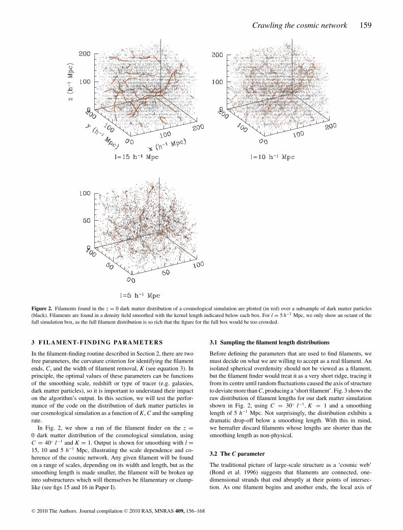
Figure 2. Filaments found in the z = 0 dark matter distribution of a cosmological simulation are plotted (in red) over a subsample of dark matter particles(black). Filaments are found in a density field smoothed with the kernel length indicated below each box. For l = 5 h−1 Mpc, we only show an octant of thefull simulation box, as the full filament distribution is so rich that the figure for the full box would be too crowded.

3 FILAMENT-FINDING PARAMETERS

In the filament-finding routine described in Section 2, there are twofree parameters, the curvature criterion for identifying the filamentends, C, and the width of filament removal, K (see equation 3). Inprinciple, the optimal values of these parameters can be functionsof the smoothing scale, redshift or type of tracer (e.g. galaxies,dark matter particles), so it is important to understand their impacton the algorithm’s output. In this section, we will test the perfor-mance of the code on the distribution of dark matter particles inour cosmological simulation as a function of K, C and the samplingrate.

In Fig. 2, we show a run of the filament finder on the z =0 dark matter distribution of the cosmological simulation, usingC = 40◦ l−1 and K = 1. Output is shown for smoothing with l =15, 10 and 5 h−1 Mpc, illustrating the scale dependence and co-herence of the cosmic network. Any given filament will be foundon a range of scales, depending on its width and length, but as thesmoothing length is made smaller, the filament will be broken upinto substructures which will themselves be filamentary or clump-like (see figs 15 and 16 in Paper I).

3.1 Sampling the filament length distributions

Before defining the parameters that are used to find filaments, wemust decide on what we are willing to accept as a real filament. Anisolated spherical overdensity should not be viewed as a filament,but the filament finder would treat it as a very short ridge, tracing itfrom its centre until random fluctuations caused the axis of structureto deviate more than C, producing a ‘short filament’. Fig. 3 shows theraw distribution of filament lengths for our dark matter simulationshown in Fig. 2, using C = 30◦ l−1, K = 1 and a smoothinglength of 5 h−1 Mpc. Not surprisingly, the distribution exhibits adramatic drop-off below a smoothing length. With this in mind,we hereafter discard filaments whose lengths are shorter than thesmoothing length as non-physical.

3.2 The C parameter

The traditional picture of large-scale structure as a ‘cosmic web’(Bond et al. 1996) suggests that filaments are connected, one-dimensional strands that end abruptly at their points of intersec-tion. As one filament begins and another ends, the local axis of



Figure 3. Length distribution for a sample of filaments found in thez = 0 smoothed dark matter distribution (smoothing kernel width ofl = 5 h−1 Mpc). The dashed line indicates the smoothing length, belowwhich filaments are removed from the sample.

structure should change the direction rapidly. The C parameter de-notes the maximum angular rate of change in the axis of structurealong a filament. If this threshold is exceeded, filament tracing isstopped.

In order to test the sensitivity of the output filaments to the valueof the C parameter, we set K = 1 and generated filament networksin the N-body simulation with a range of C. In all of these tests,

increasing the value of C led to an increase in the average length ofthe filaments and a decrease in the total number of filaments found.If the curvature criterion is not strict enough, a filament will betraced past its vertex and into another filament. Since our algorithmonly prevents filaments from starting within previously identifiedfilaments (they are allowed to cross one another), this can lead todouble detections of filaments. We can obtain a rough count of thesedouble detections by comparing filament elements to one another,where a filament element is defined as a single step (of interval, �)on the grid. In other words, for each step along a given filament, wefind the closest filament element that is not a member of that samefilament. If the closest filament element is within a smoothing lengthand has an axis of structure within C, then the original element islabelled a ‘repeat detection’. The total number of repeat detectionsin an output filament network is denoted by R. The total length ofthe network at this scale is therefore given by

Lf = (Ne − R)�, (6)

where Ne is the total number of filament elements found and �

is the step size taken by the filament finder. Non-filamentary re-gions of space have already been excluded by the criteria in equa-tion (1), so an optimum set of parameters will maximize Lf whileminimizing R.

In the left-hand panel of Fig. 4, we plot both the fraction of repeatdetections (R/Ne, dotted lines) and the total length of the network(Lf , solid lines) as a function of C. On all smoothing scales, thefraction of false positives increases steadily with increasing C, withno obvious breaks or minima. The total length, however, tends torise until it reaches a maximum, after which point it either flattens orfalls slowly. This suggests that, as long as the curvature criterion isabove a critical value, the algorithm will trace out the entire filamentnetwork. Since the fraction of false positives increases with C, wewill hereafter use a curvature criterion near this value; that is, C =50, 40 and 30◦ l−1 for l = 15, 10 and 5 h−1 Mpc, respectively.

Figure 4. Total length of the output filament network (solid lines) and the fraction of ‘repeat detections’ (dotted lines) as a function of the curvature criterion,C (left) and K (right). The value of C determines the filament ending points and the value of K determines the removal width (see equation 3). Filaments wereidentified on three different smoothing scales, l = 15 h−1 Mpc (blue), l = 10 h−1 Mpc (green) and l = 5 h−1 Mpc (red). The total length of the network (afterremoving repeat detections) maximizes at a value of C that depends on the smoothing length.



3.3 The K parameter

As each filament is found, we wish to remove from the grid asmuch of it as possible without preventing the detection of furtherreal filaments. Using the previously determined critical values of C,we ran the filament finder with a range of K and computed the totallength of the filament network and the fraction of repeat detectionsas a function of K. The results are shown in the right-hand panel ofFig. 4. All of the curves are monotonic, with repeat detections andthe network length decreasing with increasing K. Hereafter, we willset K = 1 because it yields R/Ne � 20 per cent.

3.4 Effects of sparse sampling

In real galaxy catalogues, the number of galaxies per smoothingvolume will sometimes be small and it is important to understandthe impact of shot noise on the algorithm’s ability to trace thefilament network. In a density field with sparse sampling, shotnoise will create spurious filament detections in addition to the‘repeat detections’ described in Section 3.2. We have an effectivelyshot-noise-free density field in the dark matter particle distribution(with the simulation using a mean dark matter particle density of17 particles h3 Mpc−3), so we perform sparse sampling on this fieldand use the complete particle distribution as a standard for com-parison. We construct three such data sets, sampled to densities of5 × 10−3, 2 × 10−3 and 1 × 10−3 particles h3 Mpc−3, respectively,matching the densities of the real galaxy samples to be presentedin Section 6. For each sample, we recompute the SHMAFF parame-ters and run the filament finder on all three smoothing scales, usingthe parameters derived in previous sections. We will call a ‘falsepositive’ any filament element found in the sparsely sampled datawhose nearest neighbouring element in the ‘true’ filament networkis more than a smoothing length away or does not have an axis ofstructure within an angle equal to C × l. Similarly, incompletenessis quantified by counting the filament elements in the ‘true’ networkthat have no counterparts in the sparse-sampled one.

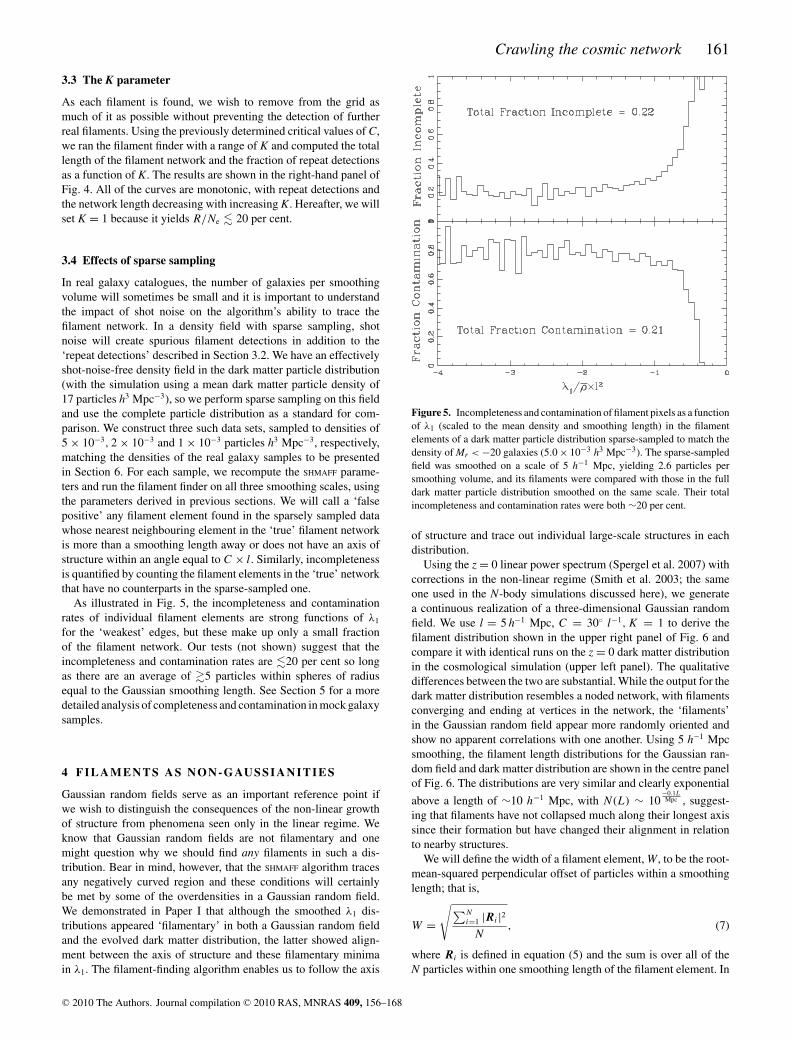
As illustrated in Fig. 5, the incompleteness and contaminationrates of individual filament elements are strong functions of λ1

for the ‘weakest’ edges, but these make up only a small fractionof the filament network. Our tests (not shown) suggest that theincompleteness and contamination rates are �20 per cent so longas there are an average of �5 particles within spheres of radiusequal to the Gaussian smoothing length. See Section 5 for a moredetailed analysis of completeness and contamination in mock galaxysamples.

4 FILAMENTS A S N ON-GAU SSIANITIES

Gaussian random fields serve as an important reference point ifwe wish to distinguish the consequences of the non-linear growthof structure from phenomena seen only in the linear regime. Weknow that Gaussian random fields are not filamentary and onemight question why we should find any filaments in such a dis-tribution. Bear in mind, however, that the SHMAFF algorithm tracesany negatively curved region and these conditions will certainlybe met by some of the overdensities in a Gaussian random field.We demonstrated in Paper I that although the smoothed λ1 dis-tributions appeared ‘filamentary’ in both a Gaussian random fieldand the evolved dark matter distribution, the latter showed align-ment between the axis of structure and these filamentary minimain λ1. The filament-finding algorithm enables us to follow the axis

Figure 5. Incompleteness and contamination of filament pixels as a functionof λ1 (scaled to the mean density and smoothing length) in the filamentelements of a dark matter particle distribution sparse-sampled to match thedensity of Mr < −20 galaxies (5.0 × 10−3 h3 Mpc−3). The sparse-sampledfield was smoothed on a scale of 5 h−1 Mpc, yielding 2.6 particles persmoothing volume, and its filaments were compared with those in the fulldark matter particle distribution smoothed on the same scale. Their totalincompleteness and contamination rates were both ∼20 per cent.

of structure and trace out individual large-scale structures in eachdistribution.

Using the z = 0 linear power spectrum (Spergel et al. 2007) withcorrections in the non-linear regime (Smith et al. 2003; the sameone used in the N-body simulations discussed here), we generatea continuous realization of a three-dimensional Gaussian randomfield. We use l = 5 h−1 Mpc, C = 30◦ l−1, K = 1 to derive thefilament distribution shown in the upper right panel of Fig. 6 andcompare it with identical runs on the z = 0 dark matter distributionin the cosmological simulation (upper left panel). The qualitativedifferences between the two are substantial. While the output for thedark matter distribution resembles a noded network, with filamentsconverging and ending at vertices in the network, the ‘filaments’in the Gaussian random field appear more randomly oriented andshow no apparent correlations with one another. Using 5 h−1 Mpcsmoothing, the filament length distributions for the Gaussian ran-dom field and dark matter distribution are shown in the centre panelof Fig. 6. The distributions are very similar and clearly exponential

above a length of ∼10 h−1 Mpc, with N (L) ∼ 10−0.1LMpc , suggest-

ing that filaments have not collapsed much along their longest axissince their formation but have changed their alignment in relationto nearby structures.

We will define the width of a filament element, W, to be the root-mean-squared perpendicular offset of particles within a smoothinglength; that is,

W =√∑N

i=1 |Ri |2N

, (7)

where Ri is defined in equation (5) and the sum is over all of theN particles within one smoothing length of the filament element. In



Figure 6. Distribution of filaments in the dark matter distribution (no sparse sampling, upper left panel) and a Gaussian random field (upper right) with the�CDM z = 0 non-linear power spectrum. The filaments are found on l = 5 h−1 Mpc scales and we only plot subsections of the full 200 h−1 Mpc boxes. In thecentre and lower panels, we show the filament length and width distributions, respectively, for the dark matter distribution (solid line) and Gaussian randomfield (dashed line). In both cases, the filament-finding algorithm was run with C = 30◦ l−1 and K = 1.

the lower panel of Fig. 6, we plot the width distributions for the twofields, again using l = 5 h−1 Mpc. The dark matter width distribu-tions are broader and are peaked at smaller widths, suggesting thatthe filaments have collapsed significantly along two of their princi-pal axes, despite having a similar length distribution. As one wouldexpect with bottom-up structure formation, the width distributionin the Gaussian random field and dark matter distribution are morediscrepant at smaller smoothing scales (other scales not shown).

4.1 Filament evolution

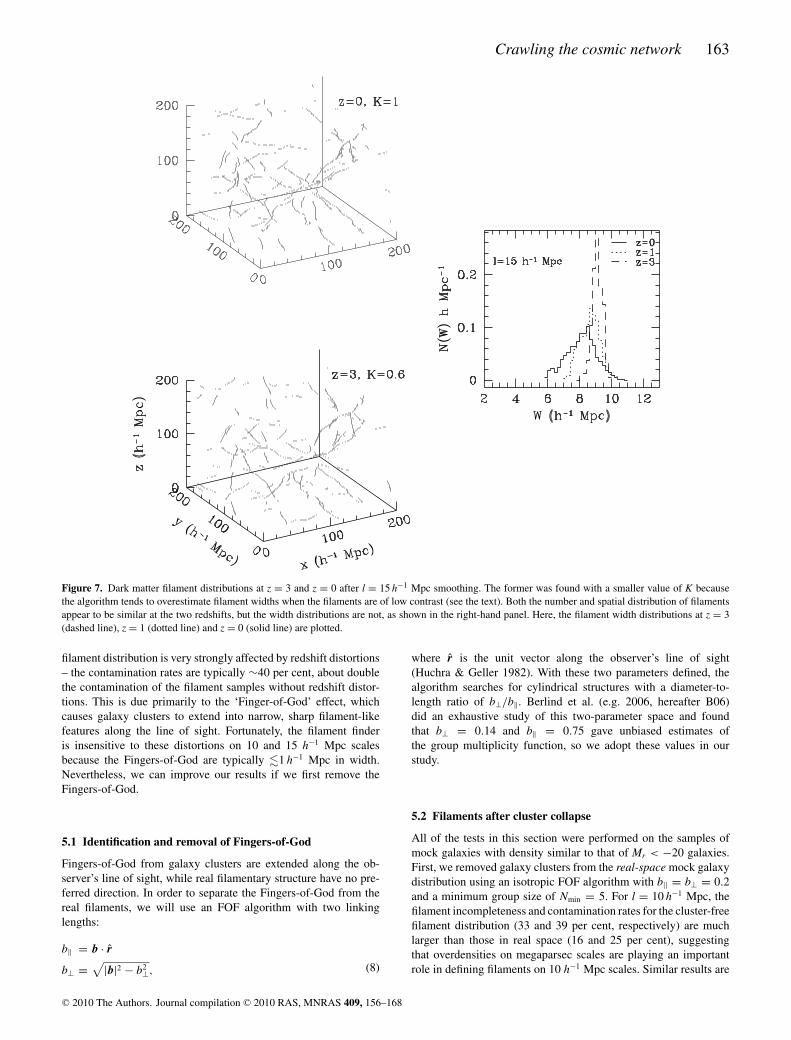
In Paper I, we showed that on a given comoving smoothing scale,there was evidence for a wall-to-filament-to-clump evolution withcosmic time. Furthermore, we showed that the axis of structurealigns with the filamentary backbone in two-dimensional slices fromcosmological simulations as early as z = 3 (see fig. 14 in Paper I).Fig. 7 shows the filament distribution at z = 0 and z = 3, now withl = 15 h−1 Mpc so as to test the largest and least-evolved structures

in the simulation box. We used a smaller removal width, K = 0.6,for the z = 3 filament distribution because the filaments are of lowercontrast than at z = 0, causing equation (3) to overestimate theirsizes. The z = 3 and z = 0 filament distributions are very similarto the eye, suggesting that the basic filament framework for l =15 h−1 Mpc is almost entirely in place at z = 3 [where 15 h−1 Mpcfluctuations have

⟨(�M/M)2

⟩1/2 ∼ 0.1]. The right-hand panel ofFig. 7 shows the filament element width distributions as a functionof redshift. As non-linear evolution proceeds, the filament widthdistributions broaden and peak at smaller widths.

5 FI L A M E N T S IN TH E M O C K G A L A X YC ATA L O G U E S

Before we proceed to identify filaments in the SDSS data, we runthe filament finder on the mock galaxy samples in redshift space(see Paper I) and compare the resulting filaments to those identifiedin the real-space z = 0 dark matter distribution. The l = 5 h−1 Mpc



Figure 7. Dark matter filament distributions at z = 3 and z = 0 after l = 15 h−1 Mpc smoothing. The former was found with a smaller value of K becausethe algorithm tends to overestimate filament widths when the filaments are of low contrast (see the text). Both the number and spatial distribution of filamentsappear to be similar at the two redshifts, but the width distributions are not, as shown in the right-hand panel. Here, the filament width distributions at z = 3(dashed line), z = 1 (dotted line) and z = 0 (solid line) are plotted.

filament distribution is very strongly affected by redshift distortions– the contamination rates are typically ∼40 per cent, about doublethe contamination of the filament samples without redshift distor-tions. This is due primarily to the ‘Finger-of-God’ effect, whichcauses galaxy clusters to extend into narrow, sharp filament-likefeatures along the line of sight. Fortunately, the filament finderis insensitive to these distortions on 10 and 15 h−1 Mpc scalesbecause the Fingers-of-God are typically �1 h−1 Mpc in width.Nevertheless, we can improve our results if we first remove theFingers-of-God.

5.1 Identification and removal of Fingers-of-God

Fingers-of-God from galaxy clusters are extended along the ob-server’s line of sight, while real filamentary structure have no pre-ferred direction. In order to separate the Fingers-of-God from thereal filaments, we will use an FOF algorithm with two linkinglengths:

b‖ = b · r

b⊥ =√

|b|2 − b2⊥, (8)

where r is the unit vector along the observer’s line of sight(Huchra & Geller 1982). With these two parameters defined, thealgorithm searches for cylindrical structures with a diameter-to-length ratio of b⊥/b‖. Berlind et al. (e.g. 2006, hereafter B06)did an exhaustive study of this two-parameter space and foundthat b⊥ = 0.14 and b‖ = 0.75 gave unbiased estimates ofthe group multiplicity function, so we adopt these values in ourstudy.

5.2 Filaments after cluster collapse

All of the tests in this section were performed on the samples ofmock galaxies with density similar to that of Mr < −20 galaxies.First, we removed galaxy clusters from the real-space mock galaxydistribution using an isotropic FOF algorithm with b|| = b⊥ = 0.2and a minimum group size of Nmin = 5. For l = 10 h−1 Mpc, thefilament incompleteness and contamination rates for the cluster-freefilament distribution (33 and 39 per cent, respectively) are muchlarger than those in real space (16 and 25 per cent), suggestingthat overdensities on megaparsec scales are playing an importantrole in defining filaments on 10 h−1 Mpc scales. Similar results are



obtained when clusters are found and removed in redshift spaceusing the approach of Section 5.1.

If we instead collapse the Fingers-of-God presented by galaxyclusters, we can remove most of the contamination without hav-ing to remove the clusters themselves. For this study, we will takethe very simple approach of moving all members of a particularcluster to their mean position; that is, we will collapse the Fingers-of-God to a point weighted by the number of galaxies in the cluster.If we follow this procedure, the incompleteness and contamina-tion are smaller (19 and 26 per cent) than the cluster-free mockgalaxy distributions and a marginal improvement over the redshift-space distribution with no special treatment of clusters (20 and27 per cent).

We repeated this exercise for filaments found on a 5 h−1 Mpcsmoothing scale. Collapsing the Fingers-of-God does lead to amarginal improvement, but filaments are still very poorly definedin redshift space at these densities, with ∼40 per cent contamina-tion rates. A more sophisticated treatment of the clusters may beneeded, but is beyond the scope of this paper. In the section thatfollows, we will discuss the application of the filament finder to realSDSS data. To minimize contamination, we will be working onlywith filaments found on 10 and 15 h−1 Mpc scales and only aftercollapsing Fingers-of-God.

6 FI LAMENTS IN THE SDSS GALAXYDI STRI BU TI ON

The SDSS has imaged a quarter of the sky in five wavebands,ranging from 3000 to 10 000 Å, to a depth of r ∼ 22.5 (York et al.2000). As of Data Release 6 (DR6; Adelman-McCarthy et al. 2008),spectra had been taken of ∼800 000 galaxies, covering 9583 deg2

and extending to Petrosian r ∼ 17.7 (Strauss et al. 2002). Galaxyredshifts are typically accurate to ∼30 km s−1, making it ideal forstudies of large-scale structure. For this study, we need a portion ofsky with relatively few coverage gaps to minimize the effect of thewindow function on the λ-space distributions. With this in mind, weconstruct two volume-limited subsamples from the northern portion(8 < α < 16 h and 25 < δ < 60) of the DR6 update of the NYUValue-Added Galaxy Catalog (NYU-VAGC; Blanton et al. 2005) thefirst 140×140×340 (h−1 Mpc)3 in size with Mr < −20.5 (Mr205)and the second 170 × 170 × 400 (h−1 Mpc)3 in size with Mr <

−21 (Mr21). The samples extend to maximum redshifts of z = 0.12and z = 0.15, respectively, and are plotted in redshift space in Fig. 8.Absolute magnitudes were computed with KCORRECT (Blanton et al.2003) using SDSS r-band Petrosian magnitudes shifted to z = 0.1(and using h = 1).

We described the compilation and processing of the SDSS sub-samples and their mock counterparts in Paper I. Before generating

Figure 8. Two volume-limited samples taken from the SDSS NYU-VAGC large-scale structure sample, with galaxies placed at their comoving positions basedon the concordance cosmology. The arrows indicate the location of the Milky Way, which is r = (310, −20, 170) h−1 Mpc and r = (400, −25, 200) h−1 Mpcin the Mr205 and Mr21 samples, respectively. The z-axes are parallel to the North Galactic Pole.



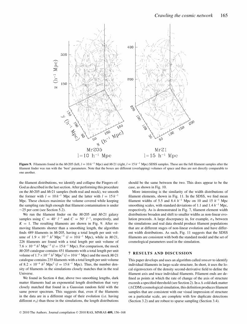
Figure 9. Filaments found in the Mr205 (left, l = 10 h−1 Mpc) and Mr21 (right, l = 15 h−1 Mpc) SDSS samples. These are the full filament samples after thefilament finder was run with the ‘best’ parameters. Note that the boxes are different (overlapping) volumes of space and thus are not directly comparable toone another.

the filament distributions, we identify and collapse the Fingers-of-God as described in the last section. After performing this procedureon the Mr205 and Mr21 samples (both real and mock), we smooththe former with l = 10 h−1 Mpc and the latter with l = 15 h−1

Mpc. These choices maximize the volume covered while keepingthe sampling rate high enough that filament contamination is under∼25 per cent (see Section 5.2).

We run the filament finder on the Mr205 and Mr21 galaxysamples using C = 40◦ l−1 and C = 50◦ l−1, respectively, andK = 1. The resulting filaments are shown in Fig. 9. After re-moving filaments shorter than a smoothing length, the algorithmfinds 489 filaments in Mr205, having a total length per unit vol-ume of 1.9 × 10−3 h2 Mpc−2 (l = 10 h−1 Mpc), while in Mr21,226 filaments are found with a total length per unit volume of7.6 × 10−4 h2 Mpc−2 (l = 15 h−1 Mpc). For comparison, the mockMr205 catalogue contains 451 filaments with a total length per unitvolume of 1.7×10−3 h2 Mpc2 (l = 10 h−1 Mpc) and the mock Mr21catalogue contains 235 filaments with a total length per unit volumeof 8.2 × 10−4 h2 Mpc2 (l = 15 h−1 Mpc). Thus, the number den-sity of filaments in the simulations closely matches that in the realUniverse.

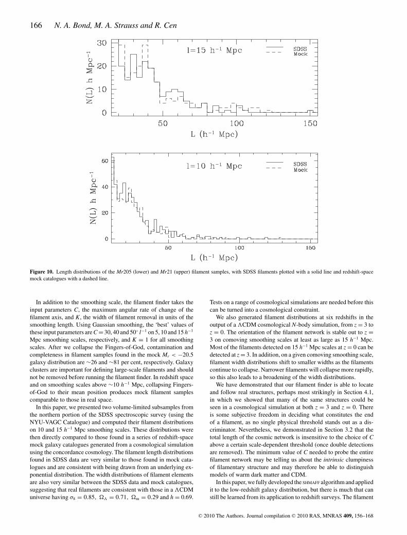
We found in Section 4 that, above two smoothing lengths, darkmatter filaments had an exponential length distribution that veryclosely matched that found in a Gaussian random field with thesame power spectrum. This suggests that, even if the filamentsin the data are in a different stage of their evolution (i.e. havingdifferent σ 8) than those in the simulations, the length distributions

should be the same between the two. This does appear to be thecase, as shown in Fig. 10.

More interesting is the similarity of the width distributions offilament elements, shown in Fig. 11. In the SDSS, we find meanfilament widths of 5.5 and 8.4 h−1 Mpc on 10 and 15 h−1 Mpcsmoothing scales, with standard deviations of 1.1 and 1.4 h−1 Mpc,respectively. As is demonstrated in Fig. 7, filament element widthdistributions broaden and shift to smaller widths as non-linear evo-lution proceeds. A large discrepancy in, for example, σ 8 betweenthe simulations and real data should produce filament populationsthat are at different stages of non-linear evolution and have differ-ent width distributions. As such, Fig. 11 suggests that the SDSSfilaments are consistent with both the standard model and the set ofcosmological parameters used in the simulation.

7 R ESULTS AND D ISCUSSION

This paper develops and uses an algorithm called SHMAFF to identifyindividual filaments in large-scale structure. In short, it uses the lo-cal eigenvectors of the density second-derivative field to define thefilament axis and trace individual filaments. Filament ends are de-fined as points at which the rate of change of the axis of structureexceeds a specified threshold (see Section 2). In a � cold dark matter(�CDM) cosmological simulation, this definition produces filamentsamples that are consistent with our visual impression of structureon a particular scale, are complete with few duplicate detections(Section 3.2) and are robust to sparse sampling (Section 3.4).



Figure 10. Length distributions of the Mr205 (lower) and Mr21 (upper) filament samples, with SDSS filaments plotted with a solid line and redshift-spacemock catalogues with a dashed line.

In addition to the smoothing scale, the filament finder takes theinput parameters C, the maximum angular rate of change of thefilament axis, and K, the width of filament removal in units of thesmoothing length. Using Gaussian smoothing, the ‘best’ values ofthese input parameters are C = 30, 40 and 50◦ l−1 on 5, 10 and 15 h−1

Mpc smoothing scales, respectively, and K = 1 for all smoothingscales. After we collapse the Fingers-of-God, contamination andcompleteness in filament samples found in the mock Mr < −20.5galaxy distribution are ∼26 and ∼81 per cent, respectively. Galaxyclusters are important for defining large-scale filaments and shouldnot be removed before running the filament finder. In redshift spaceand on smoothing scales above ∼10 h−1 Mpc, collapsing Fingers-of-God to their mean position produces mock filament samplescomparable to those in real space.

In this paper, we presented two volume-limited subsamples fromthe northern portion of the SDSS spectroscopic survey (using theNYU-VAGC Catalogue) and computed their filament distributionson 10 and 15 h−1 Mpc smoothing scales. These distributions werethen directly compared to those found in a series of redshift-spacemock galaxy catalogues generated from a cosmological simulationusing the concordance cosmology. The filament length distributionsfound in SDSS data are very similar to those found in mock cata-logues and are consistent with being drawn from an underlying ex-ponential distribution. The width distributions of filament elementsare also very similar between the SDSS data and mock catalogues,suggesting that real filaments are consistent with those in a �CDMuniverse having σ8 = 0.85, �� = 0.71, �m = 0.29 and h = 0.69.

Tests on a range of cosmological simulations are needed before thiscan be turned into a cosmological constraint.

We also generated filament distributions at six redshifts in theoutput of a �CDM cosmological N-body simulation, from z = 3 toz = 0. The orientation of the filament network is stable out to z =3 on comoving smoothing scales at least as large as 15 h−1 Mpc.Most of the filaments detected on 15 h−1 Mpc scales at z = 0 can bedetected at z = 3. In addition, on a given comoving smoothing scale,filament width distributions shift to smaller widths as the filamentscontinue to collapse. Narrower filaments will collapse more rapidly,so this also leads to a broadening of the width distributions.

We have demonstrated that our filament finder is able to locateand follow real structures, perhaps most strikingly in Section 4.1,in which we showed that many of the same structures could beseen in a cosmological simulation at both z = 3 and z = 0. Thereis some subjective freedom in deciding what constitutes the endof a filament, as no single physical threshold stands out as a dis-criminator. Nevertheless, we demonstrated in Section 3.2 that thetotal length of the cosmic network is insensitive to the choice of Cabove a certain scale-dependent threshold (once double detectionsare removed). The minimum value of C needed to probe the entirefilament network may be telling us about the intrinsic clumpinessof filamentary structure and may therefore be able to distinguishmodels of warm dark matter and CDM.

In this paper, we fully developed the SHMAFF algorithm and appliedit to the low-redshift galaxy distribution, but there is much that canstill be learned from its application to redshift surveys. The filament



Figure 11. Width distributions of the Mr205 (lower) and Mr21 (upper) filament samples, with SDSS filaments plotted with a solid line and redshift-spacemock catalogues with a dashed line. The SDSS filaments in both samples are consistent with those in the cosmological simulations, suggesting that they are insimilar stages of non-linear evolution.

evolution seen in cosmological simulations (see Section 4.1) can betested in the DEEP2 galaxy survey (Davis et al. 2003) at z ∼ 1,and the results of this comparison have already been presented inChoi, Bond & Strauss (2010). On l = 5 and 10 h−1 Mpc scales, theyconfirm a shift in the filament width distribution to smaller widthsfrom z ∼ 0.8 to 0.1, as well as a broadening of the filament widthdistribution. A possible extension of this work is a careful test ofthe �CDM cosmological model, including precision constraints oncosmological parameters, such as σ 8, and tests for primordial non-Gaussianity using the length distribution of filamentary structures.In addition, it would be useful to elaborate on the relationship oflarge-scale filaments to galaxy clusters and to explore the propertiesof galaxies in filaments relative to the general galaxy population.Finally, it would be interesting to conduct a careful search for wallsin SDSS. Paper I hinted at their presence in the data, but they wereonly present at low contrast and the λ-space distributions were notoptimal for identifying individual wall-like structures.

AC K N OW L E D G M E N T S

Funding for the SDSS and SDSS-II has been provided by the AlfredP. Sloan Foundation, the Participating Institutions, the National Sci-ence Foundation, the U.S. Department of Energy, the National Aero-nautics and Space Administration, the Japanese Monbukagakusho,the Max Planck Society, and the Higher Education Funding Councilfor England. The SDSS Web Site is http://www.sdss.org/.

The SDSS is managed by the Astrophysical Research Consor-tium for the Participating Institutions. The Participating Institu-tions are the American Museum of Natural History, AstrophysicalInstitute Potsdam, University of Basel, University of Cambridge,Case Western Reserve University, University of Chicago, DrexelUniversity, Fermilab, the Institute for Advanced Study, the JapanParticipation Group, Johns Hopkins University, the Joint Institutefor Nuclear Astrophysics, the Kavli Institute for Particle Astro-physics and Cosmology, the Korean Scientist Group, the ChineseAcademy of Sciences (LAMOST), Los Alamos National Labora-tory, the Max-Planck-Institute for Astronomy (MPIA), the Max-Planck-Institute for Astrophysics (MPA), New Mexico State Uni-versity, Ohio State University, University of Pittsburgh, Universityof Portsmouth, Princeton University, the United States Naval Ob-servatory and the University of Washington.

REFERENCES

Adelman-McCarthy J. K. et al., 2008, ApJS, 175, 297Aragon-Calvo M. A., Jones B. J. T., van de Weygaert R., van der Hulst J.

M., 2007, A&A, 474, 315Aragon-Calvo M. A., Platen E., van de Weygaert R., Szalay A. S., 2008,

preprint (arXiv:0809.5104)Berlind A. A. et al., 2006, ApJS, 167, 1 (B06)Blanton M. R. et al., 2003, AJ, 125, 2348Blanton M. R. et al., 2005, AJ, 129, 2562Bond J. R., Kofman L., Pogosyan D., 1996, Nat, 380, 603Bond N. A., Strauss M. A., Cen R., 2010, MNRAS, 406, 1609 (Paper I)



Cen R., Ostriker J. P., 1999, ApJ, 514, 1Choi E., Bond N. A., Strauss M. A., 2010, MNRAS, 406, 320Colberg J. M., Krughoff K. S., Connolly A. J., 2005, MNRAS, 359, 272Colless M. et al., 2001, MNRAS, 328, 1039Colombi S., Pogosyan D., Souradeep T., 2000, Phys. Rev. Lett., 85, 5515Dave R., Hellinger D., Primack J., Nolthenius R., Klypin A., 1997, MNRAS,

284, 607Davis M., Huchra J., Latham D. W., Tonry J., 1982, ApJ, 253, 423Davis M. et al., 2003, in Guhathakurta P., ed., Proc. SPIE Vol. 4834, Science

Objectives and Early Results of the DEEP2 Redshift Survey. SPIE,Bellingham, p. 161

de Lapparent V., Geller M. J., Huchra J. P., 1986, ApJ, 302, L1Dietrich J. P., Schneider P., Clowe D., Romano-Dıaz E., Kerp J., 2005, A&A,

440, 453Dolag K., Meneghetti M., Moscardini L., Rasia E., Bonaldi A., 2006,

MNRAS, 370, 656Eisenstein D. J., Hut P., 1998, ApJ, 498, 137Forero-Romero J. E., Hoffman Y., Gottlober S., Klypin A., Yepes G., 2009,

MNRAS, 396, 1815Gonzalez R. E., Padilla N. E., 2010, MNRAS, 407, 1449Gott J. R. I., Juric M., Schlegel D., Hoyle F., Vogeley M., Tegmark M.,

Bahcall N., Brinkmann J., 2005, ApJ, 624, 463Hahn O., Porciani C., Carollo C. M., Dekel A., 2007a, MNRAS, 375,

489Hahn O., Carollo C. M., Porciani C., Dekel A., 2007b, MNRAS, 381, 41Hahn O., Porciani C., Dekel A., Carollo C. M., 2009, MNRAS, 398, 1742Huchra J. P., Geller M. J., 1982, ApJ, 257, 423Kaiser N., Wilson G., Luppino G., Kofman L., Gioia I., Metzger M., Dahle

H., 1998, preprint (astro-ph/9809268)Massey R. et al., 2007, Nat, 445, 286

Moody J. E., Turner E. L., Gott J. R. I., 1983, ApJ, 273, 16Novikov D., Colombi S., Dore O., 2006, MNRAS, 366, 1201Pimbblet K. A., 2005, MNRAS, 358, 256Platen E., van de Weygaert R., Jones B. J. T., 2007, MNRAS, 380,

551Press W. H., Flannery B. P., Teukolsky S. A., 1986, Numerical Recipes: The

Art of Scientific Computing. Cambridge Univ. Press, CambridgeSahni V., Sathyaprakash B. S., Shandarin S. F., 1998, ApJ, 495, L5Sathyaprakash B. S., Sahni V., Shandarin S. F., 1996, ApJ, 462, L5Sathyaprakash B. S., Sahni V., Shandarin S., Fisher K. B., 1998, ApJ, 507,

L109Schaap W. E., van de Weygaert R., 2000, A&A, 363, L29Seldner M., Siebers B., Groth E. J., Peebles P. J. E., 1977, AJ, 82, 249Sheth J. V., Sahni V., Shandarin S. F., Sathyaprakash B. S., 2003, MNRAS,

343, 22Smith R. E. et al., 2003, MNRAS, 341, 1311Sousbie T., Pichon C., Courtois H., Colombi S., Novikov D., 2008a, ApJ,

672, L1Sousbie T., Pichon C., Colombi S., Novikov D., Pogosyan D., 2008b,

MNRAS, 383, 1655Spergel D. N. et al., 2007, ApJS, 170, 377Strauss M. A. et al., 2002, AJ, 124, 1810Tanaka M., Hoshi T., Kodama T., Kashikawa N., 2007, MNRAS, 379,

1546Thompson L. A., Gregory S. A., 1978, ApJ, 220, 809York D. G. et al., 2000, AJ, 120, 1579Zheng Z., Coil A. L., Zehavi I., 2007, ApJ, 667, 760

This paper has been typeset from a TEX/LATEX file prepared by the author.


crawling the cosmic network: identifying and quantifying ﬁlamentary ...€¦ · crawling the...

Documents