quality ladders in a ricardian model of trade with

Working Paper No. 81

December 2008 (Revised, April 2010)

www.carloalberto.org

THE

CARL

O AL

BERT

O NO

TEBO

OKS

Quality Ladders in a Ricardian Model of Trade with Nonhomothetic Preferences

Esteban Jaimovich

Vincenzo Merella

Quality Ladders in a Ricardian Model of Trade with

Nonhomothetic Preferences�

Esteban Jaimovich

Collegio Carlo Alberto

Vincenzo Merella

City University London

April 2010

Abstract

The literature on North-South trade has explored conditions under which international

trade might magnify income disparities between the advanced North and the backward South.

Little attention has yet been placed on the e¤ect of trade on countries that do not display

substantial dissimilarities concerning aggregate capital endowments. We show that even

when no single country is technologically more advanced than any other one and productivity

changes are uniform and identical in all countries, international trade may still be a source

of income divergence when nonhomothetic preferences and quality ladders are jointly taken

into account. Income divergence will be experienced when comparative advantages induce

patterns of specialisation that, although optimal for each country at some initial point in

time, do not o¤er the same scope for improvements in terms of subsequent quality upgrading

of �nal products.

Keywords: International Trade, Nonhomothetic Preferences, Quality Ladders

JEL Classi�cations: F11, F43

�We would like to thank Michael Ben-Gad, Jonathan Eaton, Maitreesh Ghatak, Alessio Moro, Nicola Pavoni,

Juan Pablo Rud, Stephen Wright, Fabrizio Zilibotti, and seminar participants in the Far East and South Asia

Meeting of the Econometric Society (Tokyo) and the Royal Economic Society Meeting (Surrey) for helpful com-

ments.

1

1 Introduction

In the past two decades a number of articles on international trade have started to acknowledge

the importance of nonhomothetic preferences for capturing some relevant features of North-South

trade �e.g., Flam and Helpman (1987), Stokey (1991), and Matsuyama (2000). These papers

have developed tractable models that yield patterns of specialisation where richer countries

produce and export goods with high income demand elasticity. One of the main predictions of

those models is that the impact of international trade on growth may be uneven across countries

which are at di¤erent stages in the process of development. More precisely, trade would tend

to be more bene�cial to developed economies (the North), and it may even be detrimental

to underdeveloped countries (the South). The key mechanism at work is the one originally

proposed by Prebisch (1950) and Singer (1950): as the world income rises, world aggregate

demand shifts towards the goods produced by the North, improving their terms of trade and,

thereby, magnifying initial income disparities between those richer economies and the South.

The papers mentioned above thus restrict the attention to a world economy where some coun-

tries (the North) have somehow historically accumulated larger amounts of human and physical

capital than others (the South), and show conditions under which trade magni�es initial income

disparities resulting from those capital di¤erences. However, the pattern of international special-

isation and trade might also be the source of income di¤erentials between countries that do not

display any substantial dissimilarity regarding their initial levels of human and physical capital.

In this paper, we look at economies that start o¤ with similar capital endowments, and pro-

pose a theory of uneven growth induced by trade, based on nonhomothetic preferences, quality

di¤erentiation and productive specialisation driven by Ricardian comparative advantages.

Our theory rests on �ve fundamental elements. First, there exists a large number of con-

sumption goods in the economy. Second, each speci�c type of consumption good is present in

several levels of quality, with higher qualities being increasingly costly to produce. Third, some

goods o¤er larger scope for quality upgrading than others, in the sense that it is less costly to

increase their quality. Fourth, individuals care about the quality of the goods they consume

and, moreover, their willingness to pay for higher quality of consumption increases with their

income. Fifth, countries that are similar in terms of their average productivities specialise in

the production of di¤erent goods according to their comparative advantage.

The �rst four elements above give room for nonhomothetic demand schedules, where the

income demand elasticity of every good is tied to the speci�c quality in which that particular good

2

is (optimally) traded in the market. The last element yields patterns of regional specialisation

that, combined with nonhomothetic demand schedules, may lead to divergent dynamics among

countries that are initially similar in terms of capital endowments. In such a framework, we show

that international trade may induce income divergence across countries characterised by similar

initial income levels and with no absolute advantage over one another. In particular, income

divergence will be experienced when comparative advantages dictate patterns of specialisation

that, although optimal for each speci�c country at a given stage of development, do not o¤er

the same scope for technological improvements in terms of subsequent quality upgrading of �nal

goods.

To convey some preliminary intuition of how nonhomothetic demand schedules arise as an

equilibrium result of our model, it is worth discussing in further detail some of the speci�cities

of the commodity space. In that respect, we follow the quality ladder structure featured in

Grossman and Helpman (1991) �that is, in a continuum of horizontally di¤erentiated goods, an

in�nite number of qualities for each good are available in the market. Unlike Grossman-Helpman,

however, in our framework the optimal expenditure shares across goods do not remain constant

as income changes. In particular, we postulate that the additional utility the individual derives

from a marginal increase in the quality of the goods he consumes increases with the quantity

of consumption, hence with the individual�s income (in other words, the individual�s taste for

quality increases with income). As a result, as individuals become richer they optimally shift

resources towards those goods whose quality can be set at relatively higher levels. The budget

constraint, in turn, implies that the extent by which quality can be raised for any given type

of good is related to its speci�c cost of quality upgrading. Thus, the distribution of quality

upgrading across goods results from the interplay between the underlying technological structure

and the response of the consumers�taste for quality to income variations.

In such a framework we show that, if the cost of quality upgrading di¤ers across goods, then

the shift towards higher-quality goods with rising income will (optimally) occur at di¤erent

speeds across goods. More precisely, the lower the cost of quality upgrading for a speci�c good,

the larger the quality upgrading for that good. This uneven climbing-up-the-quality-ladder will

in turn lead to nonhomothetic demand schedules, where the fraction of income spent in di¤erent

goods depends on the level of income itself.

When introduced into a general equilibrium model of international trade, the interplay be-

tween quality upgrading and comparative advantage may lead to income divergence through its

e¤ect on the terms of trade. To brie�y characterise this mechanism, take some hypothetical

3

country (call it country Z) that specialises in the production of good x, which exhibits high cost

of quality upgrading. According to the mechanism proposed in this paper, quality upgrading for

x is relatively slow as world income grows. Hence, the world expenditure share on x decreases

over time, while it shifts towards goods whose quality can be upgraded faster. As a result, as

the world income rises, Z experiences a decline in its terms of trade, because the types of goods

it produces display low income demand elasticity.

An important and novel feature of our model is the fact that quality upgrading is a phenom-

enon that occurs within types of goods, and (possibly) heterogeneously across di¤erent types

of goods. This, in turn, implies that our model generates two distinct (yet interrelated) types

of nonhomothetic behaviour: �rst, nonhomotheticity within goods arises as richer consumers

shift their expenditure towards higher-qualities of each speci�c good; second, nonhomotheticity

across goods (possibly) arises as richer consumers shift their expenditure towards goods with

larger scope for quality upgrading.1

Our open economy model predicts that richer economies specialise in the production of

goods that exhibit larger scope for quality upgrading (in turn, implying that they specialise in

the production of higher-quality goods). This prediction is in fact consistent with the evidence

presented in Khandelwal (2009). This paper estimates the length of quality ladders for di¤er-

ent industries, showing that import penetration from poorer economies in the US is lower in

industries that exhibit longer quality ladders (hence larger scope for quality upgrading), while

exports to the US originating from other developed economies tend to belong precisely to those

industries and, in particular, to the upper spectrum of their respective (long) quality ladders.2

The model also predicts that citizens from richer countries consume higher qualities than

those consumed by citizens from poorer countries. This prediction rationalises the �ndings by

Verhoogen (2008) and Iacovone and Javorcik (2009), who show that Mexican manufacturing

plants produce higher-quality goods to export to richer markets (mainly the US), and by Hallak

1Notice that we keep the word �possibly�in parenthesis for a very speci�c reason: if all goods o¤ered the same

scope of quality upgrading, then our model would no longer feature the second source of nonhomotheticity (i.e.,

expenditure shares would remain constant across types of goods with rising income).

2Schott (2004) also shows that the quality dimension within varieties of goods (measured in his paper by unit

values) is key to understand trade patterns in the world economy. In particular, he provides evidence that US

import unit values correlate positively with the exporter�s GDP per head. Moreover, this positive correlation

tends to be more pronounced for goods that exhibit larger scope for quality upgrading (e.g., manufactured goods)

compared to more homogeneous goods (e.g., natural resources goods). See also Hallak (2006) for related evidence

showing that rich countries import relatively more from countries that produce higher-quality goods.

4

and Schott (2009) who, using cross-country data, show that the quality gap in production

between rich and poor economies is smaller than their income gap, which suggests that poorer

economies are producing high-quality goods to sell in richer markets.3

Most of the existing trade literature with nonhomothetic preferences has relied on speci�-

cations that take luxuries as an exogenous category, like hierarchical or �0/1�preferences.4 An

implication of this exogeneity of luxuries is the fact that they can only deliver hump-shaped

Engel curves. By contrast, our utility speci�cation is able to let di¤erent goods behave as lux-

uries at di¤erent levels of income, and hence rationalise the highly non-monotonic shape that

observed Engel curves take, even after controlling for a number of factors such as consumers�age

and households�composition (for a short review of the �ndings about empirical Engel curves,

see Lewbel, 2006).

An exception to the above literature is a recent paper by Fajgelman, Grossman and Helpman

(2009), who provide a model of international trade with nonhomothetic preferences and di¤eren-

tiated goods, which can be o¤ered in several degrees of quality. Di¤erent from our paper, their

production technology is the same for all types of goods. Hence, nonhomotheticity is unrelated

to the heterogeneous scope for quality upgrading across goods, which is a crucial point in our

model. Finally, our paper also relates to other contributions that study Ricardian trade models

with quality ladders for a continuum of di¤erentiated types of goods, such as Taylor (1993),

Alcala (2009), and Benedetti Fasil and Borota (2009). All these contributions, however, use

homothetic speci�cations of preferences.

The paper is organised as follows. Section 2 describes the setup of the model. Section 3

presents the partial equilibrium consumer�s problem, illustrating the speci�cities of the nonho-

motheticity of demand in our model. Section 4 computes the general equilibrium in the world

economy, and analyses the e¤ects of uniform aggregate productivity growth, population growth

and income inequality within countries. Section 5 presents some illustrative empirical results

consistent with the main model�s predictions using cross-country trade data. Section 6 illustrates

our theory with a particular historical example. Section 7 concludes. The appendices contain

the omitted proofs and some additional algebraic derivations used in the main text.

3Brooks (2006) provides evidence similar to Verhoogen�s (2008) for Colombian manufacturing plants. The

same conclusion as Hallak and Schott (2009) follows from Fieler (2007), who reports that unit prices (a proxy for

quality) rise with the importer�s income per capita, even for goods from the same exporter and category.

4Further details on hierarchical preferences can be found in Bertola, Foellmi and Zweimuller (2006, pp. 302-

320). The �0/1�speci�cation of preferences is due to Foellmi, Hepenstrick and Zweimuller (2008).

5

2 Structure of the Model

We consider a world composed by two countries: the Home country and the Foreign country. For

brevity, hereafter we refer to the former as H and to the latter as F. These two economies share

a common commodity space, de�ned along two distinct dimensions: horizontal and vertical.

The �rst dimension (horizontal) designates the di¤erent types of goods (e.g., fruit products,

TVs, etc.). Di¤erent goods are indexed by the letter v along the space V � R : v 2 [0; 1].The second dimension (vertical) refers to the intrinsic quality of the good of each particular

type v (e.g., organic vs. non-organic fruit products, LCD TVs vs. cathode ray tube TVs, etc.).

For each good v 2 V, commodities are vertically ordered by the quality-index q belonging tothe set Q � R : q 2 [1;1), where a higher q denotes a higher quality. The commodity spaceis then given by the set V�Q = [0; 1] � [1;1), and each commodity is identi�ed by a pair(v; q) 2 V�Q.5

We assume that all commodities are tradable. Additionally, we assume there are no transport

costs and no tari¤s a¤ecting international trade.

2.1 Technology

In both H and F competitive �rms produce commodities based on linear production functions

in which labour represents their only variable input. Whenever it proves needed, hereafter we

adopt the following notation: unstarred symbols refer to H, starred ones to F. We let unit

labour requirements vary both across goods and across qualities of each good. Also, we let

unit labour requirements di¤er across countries. In particular, in H the unit labour requirement

for commodity (v; q) 2 V�Q is given by cvq = a (v) q�(v)=�, while in F is given by c�vq =

a� (v) q�(v)=�.

The parameter � > 0 above denotes a world aggregate-productivity parameter, which can be

interpreted as the global technology frontier. The functions a (v) and a� (v) represent good-speci�c

technological parameters, for H and F respectively, and we assume they may di¤er between those

two economies. Finally, the function �(v) summarises the cost elasticity of quality upgrading for

5 In our setup, di¤erent goods should be then understood as groups of commodities that aim at satisfying

di¤erent needs. On the other hand, di¤erent qualities of a particular good refer to the extent (or degree) in which

the need is actually satis�ed by the commodity. In that regard, food satis�es a di¤erent need when compared to

TVs (physiological nutrition vs. visual entertainment), but LCD TVs satisfy the need for visual entertainment

(objectively!) better than cathode ray tube TVs.

6

each good v, which is assumed to be the same for both H and F. Henceforth, we suppose that

a (v) : [0; 1] ! R++, where a0 (�) � 0; analogously, a� (v) : [0; 1] ! R++, where a�0 (�) � 0. Wealso assume that � (v) : [0; 1]! R++, where �0 (�) > 0 and � (0) > 1.6

In our world economy, each country will naturally specialise in those commodities they can

produce more cheaply. As a result, the international price of each commodity will be given

by pvq = min�cvqw; c

�vqw

�, where w (w�) denotes the wage in H (F), measured in a commonnumeraire. Given the unit labour requirements in the two countries speci�ed above, we can

express the international price of each commodity (v; q) 2 V�Q as follows:

pvq = � (v) q�(v)=�; (1)

where � (v) � min fa (v)w; a� (v)w�g.

2.2 Preferences and Budget Constraint

Both H and F are inhabited by a continuum of individuals with identical preferences de�ned

over the commodity space V�Q.We assume that individuals consume only one quality, denoted by qv, of each type of good

v. Let xv 2 R+ denote the consumed quantity of commodity qv (i.e., the consumed quantityof good v in quality q) by a representative individual from H. This individual�s preferences are

summarised by the following utility function:

U =

ZVlnCv dv

with Cv =

8<: xv if xv < 1

(xv)qv if xv � 1

(2)

where Cv represents a quality-adjusted consumption index.7

6From the labour requirements functions it is apparent that qualitative upgrade is costly, which seems a

natural assumption to make. Additionally, from our assumptions it follows that � (v) > 1 for all v 2 V, whichimplies that the marginal cost of improving quality is, for each good, increasing along the quality space. In

that sense, this assumption also seems quite natural, as it re�ects the fact that subsequent quality improvements

become increasingly costly. Finally, note that �0 (�) > 0, coupled with a0 (�) � 0, implies that goods are sorted

along the space V by their cost of quality upgrading.7The assumption of a single consumed quality for each good is posed to ease our exposition, and it corresponds

to the solution that arises when assuming an in�nite degree of substitution between qualities of the same goods.

More precisely, the single consumed quality would still arise if we were to consider the following utility function:

U =

ZVln

�ZQmax fxvq; (xvq)qg dq

�dv, where xvq denotes the consumed quantity of commodity (v; q) 2 V�Q.

7

The utility function captures the notion that quality is a desirable feature, and that quality

turns increasingly desirable as physical consumption rises. Notice that quality magni�es the

utility derived from (physical) consumption only when xv > 1. This last property of (2) intends

to capture the idea that individuals �rst seek to satisfy their basic consumption needs, and just

after these basic needs are met, do they start paying attention to the quality dimension of the

goods they consume.

Some additional properties about the utility function speci�ed in (2) are worth noting. First,

for each good v, marginal utility is unbounded above as consumption approaches zero, implying

that all goods will be actively consumed in an optimum. Second, considering the hypothetical

consumed quantities, xvq and xvq, of two di¤erent levels of the quality-index, q < q, for the same

good v, the marginal rate of substitution of xvq for xvq is non-decreasing along a proportional

expansion path of xvq and xvq.8 This last property of (2) allows demand functions to display

nonhomothetic behaviour, where the rich spend a larger fraction of their income in higher-

qualities than the poor.

Each individual is endowed with one unit of e¤ective labour, which is supplied inelastically.

Labour is immobile across countries. As a result, each individual in H supplies his entire labour

endowment to domestic �rms in return of a wage w 2 R++. This wage represents the onlysource of income for the individual. Therefore, his budget constraint reads as follows:Z

Vpv xv dv � w (3)

where pv 2 R++ denotes the (international) price of each unit of good qv.We de�ne �v � pvxv=w as the demand intensity of good v 2 V.9 In the optimum, given the

speci�cation in (2), the budget constraint (3) will naturally bind. It is thus straightforward to

notice that demand intensities will sum up to one across goods (i.e.,RV �vdv = 1).

All individuals in the world face the same prices for the reproducible commodities. As a

result, the analogous expressions in (2) and (3) corresponding to F read, respectively, as follows:

8To see this, note theMRS(xvq; xvq) is de�ned by (@U=@xvq) =(@U=@xvq) and, along a proportional expansion

path, xvq = k xvq, with k > 0. Then, from (2), for xvq; xvq > 1:

MRS(k xvq; xvq) =�q=q

�kq�1

�xvq�q�q

;

from where it is clear that, along the ray xvq = k xvq; MRS(xvq; xvq) is increasing in xvq.

9Demand intensities are the continuous counterpart of the discrete-case expenditure shares. Their relationship

is analogous to that between densities and discrete probabilities. We borrow this nomenclature from Horvath

(2000).

8

U� =RVmax

nxv; (xv)

q�vodv and

RV pvx

�vdv � w�. (Bear in mind that, since labour is immobile,

w and w� need not be equal.)

3 The Individual�s Optimal Consumption Choice

In this section we present the optimal consumption choice of a representative individual from

H, given the set of prices in the world economy. The results so obtained can be easily extended

to an individual from F, which is done in Appendix B.

Before stating the consumer�s optimisation problem, it proves convenient to state the follow-

ing preliminary result:

qv > 1 ) xv > 1: (4)

This result follows immediately from noting that, for all v 2 V, utility derived from consum-

ing xv 2 (0; 1] is independent of the consumed quality qv, while according to (1) the price ofcommodity qv is strictly increasing along the quality space. Given (4), we may then restate the

quality-adjusted consumption index in (2) simply as: Cv = (xv)qv .

Bearing in mind result (4) and the fact that xv = w�v=pv, the individual�s optimisation

problem can be thus stated in terms of two sets of control variables, namely fqv; �vgv2V:

maxfqv ;�vgv2V

U =

ZVqv ln

�w�vpv

�dv;

subject to:ZV�vdv = 1;

qv � 1; 8v 2 V;

pv = � (v) (qv)�(v) =�; 8v 2 V:

(5)

The �rst-order conditions corresponding to (5) are stated in the Appendix A. From those

�rst-order conditions we may obtain the following expression for each �v in the optimum:

�v = qv=Q; 8v 2 V; (6)

where Q �RV qzdz can be regarded as an aggregate index measuring the optimal consumption

bundle�s average quality. Notice that, according to (6), the fraction of income spent on good v is

determined by its optimal quality relative to the average quality of consumption. In that regard,

if all goods were optimally consumed at identical quality degrees (i.e., if qv = Q, 8v 2 V), then�v = 1 would hold for all v 2 V, and our model would behave exactly as the one by Dornbusch,Fischer and Samuelson (1977).

9

3.1 Distribution of Qualities and Demand Intensities across Goods

Given the technology in the world economy, summarised by �; � (�) and � (�), it is possible tocharacterise the distribution of the optimal qualities across goods according to their position

within the set V. Lemma 1 provides the �rst result in that direction.

Lemma 1

Consider two goods v; v 2 V, such that v < v. Then: qv � qv; with strict inequality i¤ qv > 1.

Proof. See Appendix C.

Lemma 1 implies that the consumed quality qv is non-increasing in the good-index v. The

underlying intuition for Lemma 1 is straightforward: those goods which can be more cheaply

upgraded tend to be optimally consumed in higher quality degrees.

The monotonicity of qv implied by Lemma 1 allows us to split the goods space in two disjoint

subsets. The �rst subset containing goods that are bound to be consumed at the baseline quality

(i.e., qv = 1) � these are the higher-indexed goods. The second one comprising the goods for

which the constraint qv � 1 in (5) does not bind in the optimum �these are the lower-indexed

goods. Henceforth, we denote the second subset by L � V.Lastly, regarding the distribution of the demand intensities, from the condition in (6) we can

observe that, in the optimum, demand intensities are set proportional to the optimal qualities.

As a result, the distribution of �v across goods will qualitatively mirror that of qv.

3.2 E¤ects of Aggregate Productivity Growth on Demand

In this section we study the e¤ects of letting the parameter � vary, while holding unchanged

the functions a (�), a� (�) and � (�), along with w and w�. The consequence of this is letting theconsumer�s real income increase, without altering any of the relative prices of commodities in

the space V�Q.For su¢ ciently low levels of aggregate productivity, the subset of goods consumed at the

baseline quality initially comprises the entire set V; formally, L = ; holds when � is below thethreshold � � a (0) exp (� (0)). As world aggregate productivity rises beyond the threshold �,

the subset L starts expanding, and eventually L = V holds when � is su¢ ciently large.10

The next lemma complements Lemma 1 and describes in further detail how optimal qualities

evolve as the parameter � changes.10For a formal proof of these results, see Lemma 3 in Appendix D.

10

Lemma 2

Let L = fv 2 V : �v = 0g, where �v is the Lagrange multiplier associated to the constraint qv � 1.Consider two goods v; v 2 V, such that v < v. Then:

i) 8� 2 (0; �) ) @qv=@� = @qv=@� = 0;

ii) 8� � � ) @qv=@� � @qv=@�; with strict inequality if v 2 L.


Lemma 2 shows that, whenever L is non-empty (i.e., case ii in the lemma), for all goods

belonging to L the consumed quality increases when world aggregate productivity rises. Fur-

thermore, this e¤ect is stronger for those goods whose quality can be more cheaply upgraded

�i.e., those goods carrying a lower � (v). On the other hand, we can observe that the optimal

quality of goods that do not belong to L does not respond to (in�nitesimal) changes in �.

We can accordingly identify two distinct regimes depending on the level of � that prevails.

First, we refer to an economy with � � � as a subsistence economy. In a subsistence economy,all goods are consumed at the baseline quality. Second, we refer to an economy with � > � as

a modern economy. In a modern economy some goods (and possibly all of them) are consumed

strictly above the baseline quality.

In what follows we proceed to further characterise these two regimes.

Subsistence Economy: � � �

In this regime, qv = 1 holds for all v 2 V. This in turn means that Q = 1 and �v = 1

must hold for all v 2 V as well. Thus, in a subsistence economy demand intensities remain

constant and equal to one for all goods as � increases.11 In that regard, a subsistence economy

displays analogous behaviour to the economy discussed in Dornbusch et al (1977), where demand

schedules are homothetic across types of goods.

Modern Economy: � > �

This regime is characterised by qv > 1 for all v 2 [0; ~v(�)), where ~v(�) denotes the thresholdv 2 V such that qv > 1 for all v < ~v(�). Hence, the average quality can be written as Q =

1 � ~v (�) +R ~v(�)0 qz dz, from where it follows that @Q=@� =

R ~v(�)0 (@qz=@�) dz > 0. Since

@qv=@� = 0 for all v =2 L, then because of (6), @�v=@� < 0 must hold for all v =2 L. As a11 It must be noted that this result applies only if � � � holds after performing the comparative statics exercise.

11

result, given thatRV �v dv = 1, it must thus be the case that the demand intensities of some

(and possibly all) v 2 L will increase as � rises. Henceforth, let J � V denote the subset of Vcomprising all those goods for which @�v=@� > 0.

In a subsistence economy, J = ;, while in a modern economy, J 6= ;. In other words, in amodern economy the homotheticity of demand intensities across goods no longer holds, as a

subset of goods whose income demand elasticity is larger than one shows up. Notice, too, that

J � L, since @qv=@� > 0 is a necessary condition for @�v=@� > 0 to hold.The next proposition further characterises the behaviour of the demand intensities, �v, as �

rises.

Proposition 1

Let J = fv 2 V : @�v=@� > 0g. Consider two goods v; v 2 V, such that v < v. Then:

i) 8� 2 (0; �) ) @�v=@� = @�v=@� = 0;

ii) 8� � � ) @�v=@� � @�v=@�; with strict inequality if v 2 J


To interpret our previous results more clearly, notice that J may be understood as the set

of luxury goods, where by luxury goods we refer to those goods whose income demand elasticity

is larger than 1. Since the set J always comprises lower-indexed goods, the luxury goods are

exactly those goods whose quality qv is relatively high compared to the average quality Q: In

that regard, in our model it is the (relative) quality that determines whether or not a particular

goods is luxurious.

Figure 1 illustrates this feature graphically. The distributions of qualities and demand in-

tensities across goods are drawn for four di¤erent levels of world aggregate-productivity (�0 �� < �1 < �2 < �3). When individuals are still poor (i.e., for a level of productivity �0 � �),

satisfying all basic needs constitutes their main goal, leading them to keep the quality of all

goods at the baseline and setting accordingly equal demand intensities for all goods. As indi-

viduals become richer, some goods � for a level of productivity �1 2 (�0; �2)� and eventually

all goods � for a level of productivity �3 � �2� are consumed in higher qualities. As a result,

for those three levels of �, a subset of goods with �v > 1 appears in the lower spectrum of the

(unit) goods set. Additionally, the goods whose quality is relatively higher attract increasingly

larger income shares, as given the preference speci�cation in (2) individuals tend to value high-

quality commodities relatively more as they become wealthier. This last point is formalised in

the following corollary.

12

Figure 1: Distribution of qualities and demand intensities across goods

qv

v1

q.(κ3)

0

βv

v10

q.(κ0)

q.(κ1)

q.(κ2)

β.(κ3)

β.(κ2)

β.(κ1)β.(κ0)

Corollary 1

Let # (v) �R v0 �z dz. Then:

(i) 8� 2 (0; �) ) @# (v) =@� = 0; 8v 2 V;

(ii) 8� � � ) @# (v) =@� � 0; 8v 2 V; with strict inequality if v < 1.


Corollary 1 synthesizes the eventual nonhomothetic behaviour of the demand schedules im-

plied by our model. More precisely, whenever � < �, demand schedules are homothetic across

goods. However, when � lies above the threshold �, income starts being spent in growing

proportion on lower-indexed goods.

4 General Equilibrium in the World Economy

In Section 3, we have studied the optimal consumption choice of an individual from H, taking

the wages in H and in F, w and w�, as exogenously given. (In Appendix B, we do the same for

the case of an individual from F.) These wages in turn determine the prices of all reproducible

commodities in the world economy through equation (1). Our former analysis has therefore

yielded only partial equilibrium results.

13

The present section computes the general equilibrium in this world economy. This requires

endogenising wages and, thereby, the prices of all reproducible commodities. Given that in a

general equilibrium only relative prices are determined, we henceforth take the wage in F as the

numeraire, by setting w� = 1.

So far we have not put any structure in terms of comparative advantage. The next assumption

dictates the pattern of comparative advantage across countries.

Assumption 1 Let A (v) � a� (v) =a (v). We suppose: (i) A0 (v) < 0, and (ii) 9 v0 2 (0; 1) :A (v0) = 1.

Assumption 1 represents the only source of heterogeneity across countries in our model. In

particular, this last assumption implies that H enjoys a comparative advantage in the production

of lower-indexed commodities, while F has a comparative advantage in the production of upper-

indexed commodities.

Note that given the cost functions cvq and c�vq speci�ed in section 2.1, because � (v) is the

same for H and F, the nature of comparative advantage does not change as we move up in

the quality ladder.12 In that sense, in the model, the comparative advantage always refers to

particular goods, irrespective of the quality at which those goods are actually produced (for

example, a country that has a comparative advantage in producing fruit products, will have this

advantage both in organic and in non-organic fruit products).

From the international pricing equation (1) and Assumption 1, we can derive the marginal

good m (that is, the good that can be supplied by both countries at the same price), which

satis�es:

A (m) = w=w�: (7)

Equation (7) implies that, given the relative wage w=w�, H will produce all the goods in the

interval [0;m] and F will produce all the goods within [m; 1].

In order to allow countries to possibly display identical income per head in equilibrium (that

is, in order to remove any direct source of absolute advantage from the model), we pose the next

assumption, which formally states symmetry in terms of countries�comparative advantage.

Assumption 2 (Symmetric comparative advantages) We suppose: v0 = 0:5.

12Letting � (�) vary across countries change in a similar fashion as a (�) would not qualitatively alter the resultsof the paper � in fact, adding heterogeneity on � (�), on top of that on a (�), would reinforce our �ndings.

14

Additionally, to disregard the e¤ects of heterogeneous population size in di¤erent countries,

we initially suppose that both H and F are inhabited by a continuum of individuals with identical

mass, which we normalise to one. (We explore the general equilibrium e¤ects of heterogenous

population size later on in Section 4.2.)

A representative individual from H will then solve:

maxfqv ;�vgv2V

U =

Z m

0qv ln

�v�

a (v) q�(v)v

!dv +

Z 1

mqv ln

�v�w

a� (v) q�(v)v

!dv;

subject to:ZV�v dv = 1; and qv � 1; 8v 2 V:

(8)

On the other hand, a representative individual from F solves:

maxfq�v ;��vgv2V

U� =

Z m

0q�v ln

��v�

a (v) q�(v)v w

!dv +

Z 1

mq�v ln

��v�

a� (v) q�(v)v

!dv;

subject to:ZV��v dv = 1; and q

�v � 1; 8v 2 V:

(9)

The solution of (8) and (9) yields the demand functions of each good v 2 V by H and F,

respectively. By using # (v) �R v0 �z dz (as de�ned in Corollary 1) and #

� (v) �R v0 �

�zdz (see

Corollary 2 in Appendix B), we can write the equilibrium condition for the market of goods

produced in H as follows:

# (m)w + #� (m) = w; (10)

wherem is the marginal good as de�ned by (7). Condition (10) essentially says that the aggregate

amount of income spent by the world in goods produced in H must be equal to the aggregate

income of H. This condition can also be understood as the equilibrium condition for the labour

market in H.13

The world economy general equilibrium is determined by (7), (8), (9), and (10). Henceforth,

we will focus our attention on the equilibrium values of w and m, and on how these two variables

respond to some comparative statics experiments commonly explored by the previous literature

on international trade with nonhomothetic preferences. Firstly, we analyse the general equilib-

rium consequences of uniform aggregate productivity growth in the world economy; this exercise

shows how our model can account for income divergence across countries with similar initial con-

ditions purely via the endogenous evolution of the terms of trade. Secondly, we investigate the13Because of the Walras�Law, an analogous condition can be derived for the equilibrium in the labour market

in F.

15

e¤ects of uneven population growth across countries, and illustrate how the country in which

population grows faster tends to experience a decline in its terms of trade and relative income.

Lastly, we look at the case of income inequality within countries, and discuss how inequality

tends to improve the terms of trade and the relative income of the economy that specialises in

producing goods that display higher income demand elasticity, regardless of whether inequality

arises in H or F.

4.1 Worldwide Uniform Aggregate Productivity Growth

In this subsection, we look at the impact of changes in � on the equilibrium values of w and m.

We can split the results in two di¤erent cases.

Subsistence economies: � � �

From our previous discussion, we can observe that when � � �, the optimal demand intensitiesare set at �v = ��v = 1 for all v 2 V. This result in turn implies that # (m) = #� (m) = m.

Therefore, (10) simpli�es to:

w = m= (1�m) : (11)

Combining (7) with (11), leads to m= (1�m) = A (m), from where it follows that, for all � � �:w = 1 and m = 0:5. That is, H and F exhibit the same level of income, and the pattern of

regional specialisation is accordingly dictated by the �natural�comparative advantage of each

country without the relative-wage e¤ect (i.e., those that derive purely from Assumption 1).14

Modern economies: � > �

When aggregate productivity is su¢ ciently high, the income equality between H and F no longer

holds. In particular, as � rises above the threshold �, the terms of trade start moving in favour

of H, and thus H becomes relatively richer than F. Moreover, the income disparity between H

and F further increases as � keeps rising.

Proposition 2

Let � > �. Then, in equilibrium:

14Notice that, since w = 1 for all � � �, in fact � = �� (that is, the threshold on � that divides a subsistence-economy from a modern economy happens to be the same for both H and F). As a consequence, we can refer to

both thresholds simply as �.

16

(i) w > 1; m < 0:5;

(ii) @w=@� > 0; @m=@� < 0:

Proof.

Part (i). When � > �, from Corollary 1 and 2 it follows that #(m) > m and #�(m) > m. As a

result, by using (10), we can obtain:

w =#�(m)

1� #(m) >m

1�m: (12)

Combining next (12) with (7), and recalling Assumption 1 and 2 leads to:

A(m) =#�(m)

1� #(m) >m

1�m , m < 0:5.

Finally, since m < 0:5, equation (7) implies that w > 1:

Part (ii). Next, to study how w and m vary as � keeps rising above �, we di¤erentiate the

equilibrium conditions (7) and (10). This leads to:

@w

@�= A0(m)

@m

@�(13)

and

(w�m + ��m)@m

@�+

�w@#(m)

@w+ #(m) +

@#�(m)

@w

�@w

@�+

�@#(m)

@�+@#�(m)

@�

�=@w

@�; (14)

where the �rst term in (14) uses the fact that @#(m)=@m = �m and @#�(m)=@m = ��m. Plugging

(13) into (14), we can obtain:

@m

@�=

@#(m)=@�+ @#�(m)=@�

[1� #(m)� w @#(m)=@w � @#�(m)=@w]A0(m)� (w�m + ��m): (15)

For determining the sign of (15), we can use the following two results: �rst, Corollary 1 states

that both @#(m)=@� > 0 and @#�(m)=@� > 0; second, as shown in Appendix D, @#(m)=@w � 0and @#�(m)=@w < 0. Therefore, since 1 � #(m) > 0 and A0(m) < 0, then @m=@� < 0 obtainsfrom the right-hand side of (15). Finally, from (13) it then follows that @w=@� > 0.

Proposition 2 shows that as the world aggregate-productivity parameter, �, increases, the

income in H eventually begins diverging away from the income in F. The reason for the divergence

rests on the fact that H enjoys a comparative advantage in producing lower-indexed goods, which

tend to be consumed in relatively higher qualities and display accordingly higher income demand

elasticity. As a consequence, as the world productivity grows uniformly above �, aggregate world

17

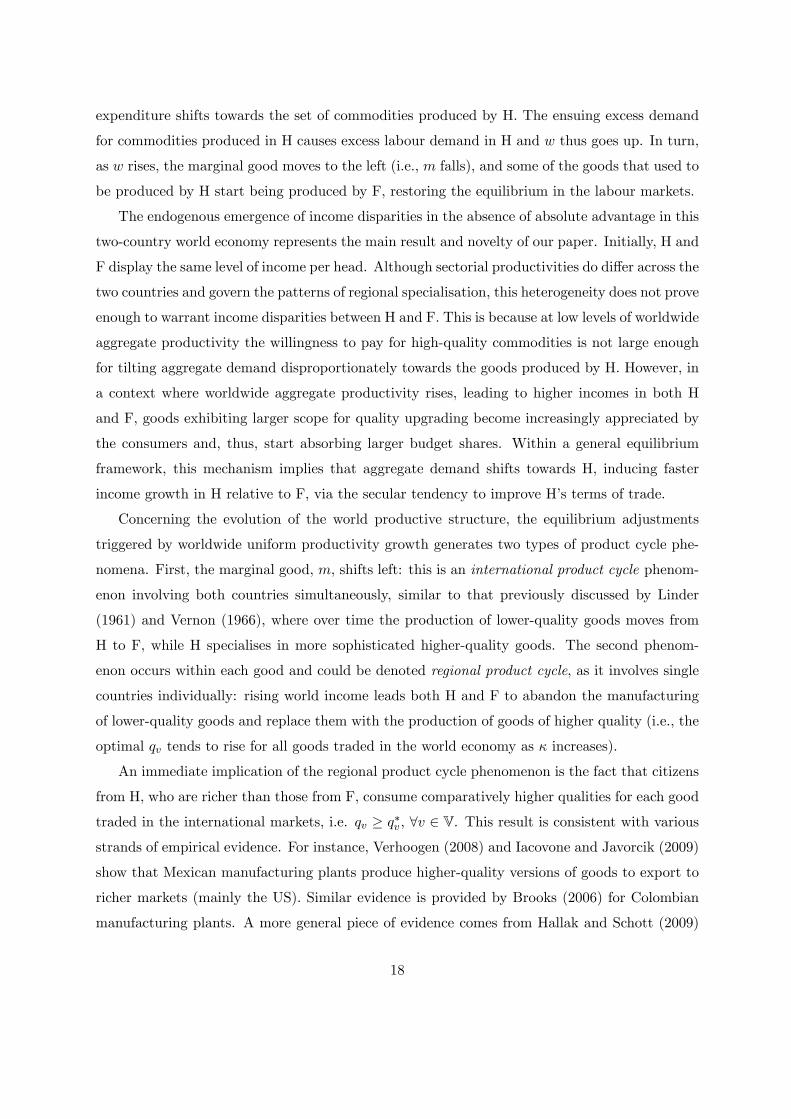
expenditure shifts towards the set of commodities produced by H. The ensuing excess demand

for commodities produced in H causes excess labour demand in H and w thus goes up. In turn,

as w rises, the marginal good moves to the left (i.e., m falls), and some of the goods that used to

be produced by H start being produced by F, restoring the equilibrium in the labour markets.

The endogenous emergence of income disparities in the absence of absolute advantage in this

two-country world economy represents the main result and novelty of our paper. Initially, H and

F display the same level of income per head. Although sectorial productivities do di¤er across the

two countries and govern the patterns of regional specialisation, this heterogeneity does not prove

enough to warrant income disparities between H and F. This is because at low levels of worldwide

aggregate productivity the willingness to pay for high-quality commodities is not large enough

for tilting aggregate demand disproportionately towards the goods produced by H. However, in

a context where worldwide aggregate productivity rises, leading to higher incomes in both H

and F, goods exhibiting larger scope for quality upgrading become increasingly appreciated by

the consumers and, thus, start absorbing larger budget shares. Within a general equilibrium

framework, this mechanism implies that aggregate demand shifts towards H, inducing faster

income growth in H relative to F, via the secular tendency to improve H�s terms of trade.

Concerning the evolution of the world productive structure, the equilibrium adjustments

triggered by worldwide uniform productivity growth generates two types of product cycle phe-

nomena. First, the marginal good, m, shifts left: this is an international product cycle phenom-

enon involving both countries simultaneously, similar to that previously discussed by Linder

(1961) and Vernon (1966), where over time the production of lower-quality goods moves from

H to F, while H specialises in more sophisticated higher-quality goods. The second phenom-

enon occurs within each good and could be denoted regional product cycle, as it involves single

countries individually: rising world income leads both H and F to abandon the manufacturing

of lower-quality goods and replace them with the production of goods of higher quality (i.e., the

optimal qv tends to rise for all goods traded in the world economy as � increases).

An immediate implication of the regional product cycle phenomenon is the fact that citizens

from H, who are richer than those from F, consume comparatively higher qualities for each good

traded in the international markets, i.e. qv � q�v , 8v 2 V. This result is consistent with variousstrands of empirical evidence. For instance, Verhoogen (2008) and Iacovone and Javorcik (2009)

show that Mexican manufacturing plants produce higher-quality versions of goods to export to

richer markets (mainly the US). Similar evidence is provided by Brooks (2006) for Colombian

manufacturing plants. A more general piece of evidence comes from Hallak and Schott (2009)

18

who using cross-country data show that the quality gap in production between rich and poor

economies is smaller than their income gap, which suggests that poorer economies are producing

high-quality goods to sell in richer markets. The same conclusion follows from Fieler (2007) who

reports that unit prices (a proxy for quality) rise with the importer�s income per capita, even

for goods originating from the same exporter and commodity category.

As a �nal remark, notice that the proof of result (ii) in Proposition 2, which states that

wages rise and the marginal good shifts leftwards as world aggregate-productivity increases, does

not rely on Assumption 2 at any moment. In fact, both @w=@� > 0 and @m=@� < 0 would still

obtain if we instead gave a larger range of initial advantage to F by assuming that �0 < 0:5. If

�0 < 0:5, somewhat richer dynamics would be obtained, though. More precisely, w < 1 would

hold for levels of worldwide productivity below a certain (�nite) threshold b� > �, while the

model would predict catching-up by H for values of � 2 (�; b�), followed next by overtaking anddivergence in an analogous fashion as it occurred when �0 = 0:5.

4.2 Uneven Population Growth

In this subsection we let the population size in F di¤er from that in H. In particular, we let the

total mass of individuals in F equal L > 1, while we keep the total mass of individuals in H

equal to 1. Thus, the labour market equilibrium condition in H will be given by:

#(m)w + L#�(m) = w: (16)

Visual inspection on (16) and (10), combined with (7), immediately implies that the equi-

librium value of w that is delivered by (16) will be strictly larger than that yielded by (10).

In particular, in equilibrium w > 1, regardless of the value of �. Furthermore, this source of

income disparity between F and H magni�es as the value of L rises. This is because, when the

population in F increases, the relative wage w must go up so as to accommodate the excess

supply of labour in F. More precisely, a larger L requires more goods to be produced by F in

order to keep full employment there; this is accomplished by letting w go up, which in turn

shifts the marginal good m to the left, helping restore the equilibrium in the labour markets.

The result that, as the relative population of F increases, the H relative wage rises is in

line with the models in Flam and Helpman (1987), Stokey (1991) and Matsuyama (2000).

However, some interesting di¤erences are also present. In Flam-Helpman and Stokey, although

the optimal bundle of goods traded in the market changes, no new goods actually appear in the

world economy as w rises due to uneven population growth in the world. In Matsuyama, new

19

goods start being produced, but this happens only in the country whose population grows slower

(i.e., in H); the country whose population grows faster, F, does not introduce new goods into

the world markets, but only takes on the production of (some) goods that are abandoned by H

as w increases. In our model, new goods actually start being produced by F as its relative wage

decreases owing to faster population growth. A higher w brings about two di¤erent e¤ects: �rst,

individuals in H become richer (income e¤ect); second, the relative prices of the goods originally

produced in F decline (substitution e¤ect). Taken jointly, these two e¤ects reinforce one another

and induce individuals from H to start demanding higher qualities for the goods produced in

F.15

4.3 Income Inequality within Countries

In this subsection we discuss the general equilibrium consequences of introducing some degree

of income heterogeneity within countries. Here, analogous qualitative results are generated

regardless of whether inequality is introduced in F or H (or in both at the same time). Therefore,

for brevity, in what follows we focus only on the �rst case.

Assume that F is inhabited by two types of individuals: p and r, where the p stands for

poor and r stands for rich. Each sub-group of individuals from F has mass equal to 0:5. The

di¤erence between the two sub-groups lies in that a type p is endowed with a smaller amount

of e¤ective labour than a type r. In particular, suppose that type-p individuals are endowed

with 1� � units of e¤ective labour and individuals in r are endowed with 1+ � units of it, where� 2 (0; 1). On the other hand, in H everyone is endowed with the same amount of e¤ective

labour. Introducing income inequality in the model leads to interesting results when the types

p are so poor that, in equilibrium, they consume all goods at the baseline quality level, whereas

in contrast the types r can a¤ord consuming at least some of the goods strictly above that level.

To focus on such case, we accordingly set � = �.

Introducing income inequality in F raises the relative wage in H. This is owing to the nonho-

motheticity of the demand schedules of the rich foreigners. More precisely, increasing � transfers

income from the poor foreigners, who spend a fraction m of it in goods from H, to the rich

foreigners, who spend a fraction #�r(m) > m of their income on those commodities. As a result,

aggregate demand for goods produced in H rises, leading to higher w. Similarly, it is quite15For example, our model then predicts that Africa will start to produce, say, organic bananas to sell in Europe,

as increasingly richer European consumers begin desiring to purchase higher-quality fruit products, which are

moreover becoming relatively cheaper over time as population in Africa grows faster than in Europe.

20

straightforward to observe that incorporating inequality in H would carry similar consequences

on w and m. This is the case because the rich locals would tend to shift demand towards the

goods produced in H; exactly the same shift induced before by the presence of rich foreigners.

5 Length of Quality Ladders and Exports Behaviour: a brief

examination of the trade data

In this section, we conduct a few empirical exercises to assess whether the central predictions

of our model �nd some empirical support in the trade data. More speci�cally, our aim is to

determine whether the exports, both at a world- and country-level of aggregation, correlate with

world income changes in a way that is consistent with our previous theoretical �ndings. For this

purpose, we propose two stylised reduced-form approaches to assess our predictions. The �rst

approach, illustrated in Section 5.2, looks at whether long-ladder goods attract increasing world

expenditure shares with rising world income. The second approach, illustrated in Section 5.3,

investigates whether exports from countries specialising in the production of long-ladder goods

increase relatively more when world income rises. Furthermore, we look at how economies�initial

specialisation correlates with future exports growth in a context of world income growth, in the

attempt to investigate whether the initial pattern of specialisation may lead to uneven future

exports growth when goods di¤er in their scope for quality upgrading.

5.1 The Length of Quality Ladders Across Goods

The �rst step is to construct a proxy for the length of quality ladders across a large set of di¤er-

ent types of tradeable goods. We build two di¤erent proxies based on measures of dispersion of

import unit prices using the data compiled by Feenstra et al (2005). This dataset documents bi-

lateral trade at the country level for the period 1962-2000 measured both in value and quantities,

organised following the 4-digit Standard International Trade Classi�cation (SITC-4), Revision

2. From this dataset, we calculate the (average) import unit prices of each SITC-4 product by

each importer during the year 2000.16 As a result, we are able to obtain up to 182 di¤erent unit

16We choose to calculate unit prices using only the year 2000 for two di¤erent reasons. First, it avoids problems

that may arise from comparing unit prices at di¤erent points in time. Second, and more importantly, using the

last year available seems the most promising one in terms of proxying the length of ladders according to the

nature of nonhomotheticities in our model. This is because the poorest country in 2000 was roughly as poor as

the poorest one in 1962, whereas the richest economy in 2000 was substantially richer than the richest one in

21

prices (one for each importer) for each of the 749 di¤erent goods in the SITC-4 categorisation.

In order to construct our �rst proxy for the length of quality ladders, we sort the (average)

import unit prices obtained for every importer, and pick the maximum and minimum for each of

the 749 goods in the SITC-4 categorisation. We next use these two boundary prices to compute

the max-to-min price ratio for every SITC-4 good. In that regard, unit prices of each SITC-4

good are taken as proxies for the intrinsic qualities of that particular good, and the max-to-min

price ratios are accordingly viewed as proxies for the length of quality ladders of goods.17

To obtain our second proxy for the length of quality ladders, we compute the coe¢ cients of

variation of the distribution of unit prices for each of the SITC-4 goods.18 The underlying idea

for this measure is that goods featuring longer quality ladders should, in general, also display a

more �dispersed�distribution of unit prices.19

In Table 1 we group all the SITC-4 sectors/goods into their corresponding 1-digit sector.

Therein we report the average values of the max-to-min unit price ratios and the average values

of coe¢ cients of variation of unit prices. With the exception of sector 2, Table 1 seems to point

to the common perception that the quality ladders of primary goods tend to be shorter than

those of manufacturing products (i.e. sectors 5 to 8). Sector 9, which contains only 5 products

in the SITC-4 classi�cation, appears to be an outlier when compared to the other sectors.

1962. (In 1962 the poorest and richest economies were Guinnea Bissau and Switzerland with GDP per head 417

and 19512, respectively, measured in PPP 2005 US dollars. In 2000, the poorest was Zaire with GDP per capita

equal to 312 and the richest was Luxemburg with 63419, both measured in PPP 2005 US dollars.)

17 In order to mitigate the e¤ect of outliers and measurement errors, when computing the max-to-min price

ratios we clean the data on unit prices along two di¤erent dimensions: i) we disregard unit prices from importers

whose reported import quantities of those particular SITC-4 goods equals 1; ii) we disregard the lowest price

when the second-lowest recorded unit price is more than 100% larger than the former and, similarly, we disregard

the highest price if this one more than doubles the second-highest recorded unit price (when this occurs, we utilise

the second-lowest or second-highest unit prices to build the extreme price ratios).

18 In this case, we also clean the data of import unit prices following the same two procedures stated in the

previous footnote.19As mentioned previously in the Introduction, unit prices/values have been used before as proxies of quality

in the empirical trade literature: e.g., Schott (2004), Hallak (2006), Fieler (2007). Of course, unit prices/values

should only be taken as an imperfect proxy of the intrinsic quality of the commodity, since factors other than

quality may also be a¤ecting unit prices (for example, the degree of horizontal di¤erentiation across industries,

heterogeneous transport costs, trade tari¤s).

22

Table 1: Averages at 1digit level of disaggregationNumber of Average of Average ofproducts in maxtomin coeff. of variation

SITC4 classif. unit price ratios of unit prices

0 Food and live animals 93 46.7 0.7111 Beverages and tobacco 11 25.1 0.6562 Crude materials, inedible, except fuels 101 134.6 1.0843 Mineral fuels, lubricants and rel. materials 20 44.6 0.8764 Animal and vegetable oils, fats and waxes 18 11.8 0.5265 Chemicals and related products 91 177.8 1.0246 Manufactured goods classified chiefly by material 175 102.7 0.9527 Machinery and transport equipment 157 186.1 0.9198 Miscellaneous manufactured articles 78 100.8 0.8879 Commodities and trans. not classified elsewhere 5 1450.7 2.309

ALL GOODS 749 130.6 0.927

SITC1 Sector

5.2 Cross-Good Regressions

One of the main predictions of our model is that goods with lower cost of quality upgrading tend

to feature longer quality ladders and exhibit higher income demand elasticities. As a result, long-

ladder goods will tend to attract increasing world expenditure shares with rising world income.

We assess this prediction on a reduced-form approach by running the following regression:

�Xj;t = �+ � (�Yw;t � Ladderj) + �t + "j;t; (17)

where �Xj;t is the percentage growth of the total value of world exports (and imports) of

good j in year t, �Yw;t is the percentage growth of world income per head in year t, and the

variable Ladderj denotes the length of the quality ladder of good j. Our model thus predicts

� > 0 because goods with larger scope for quality upgrading should also display higher income

demand elasticities. Notice that since (17) includes year �xed e¤ects (�t), we do not need to

include �Yw;t as another independent variable because such e¤ect will be fully captured by each

�t (more precisely, �Yw;t and �t are perfectly colinear).

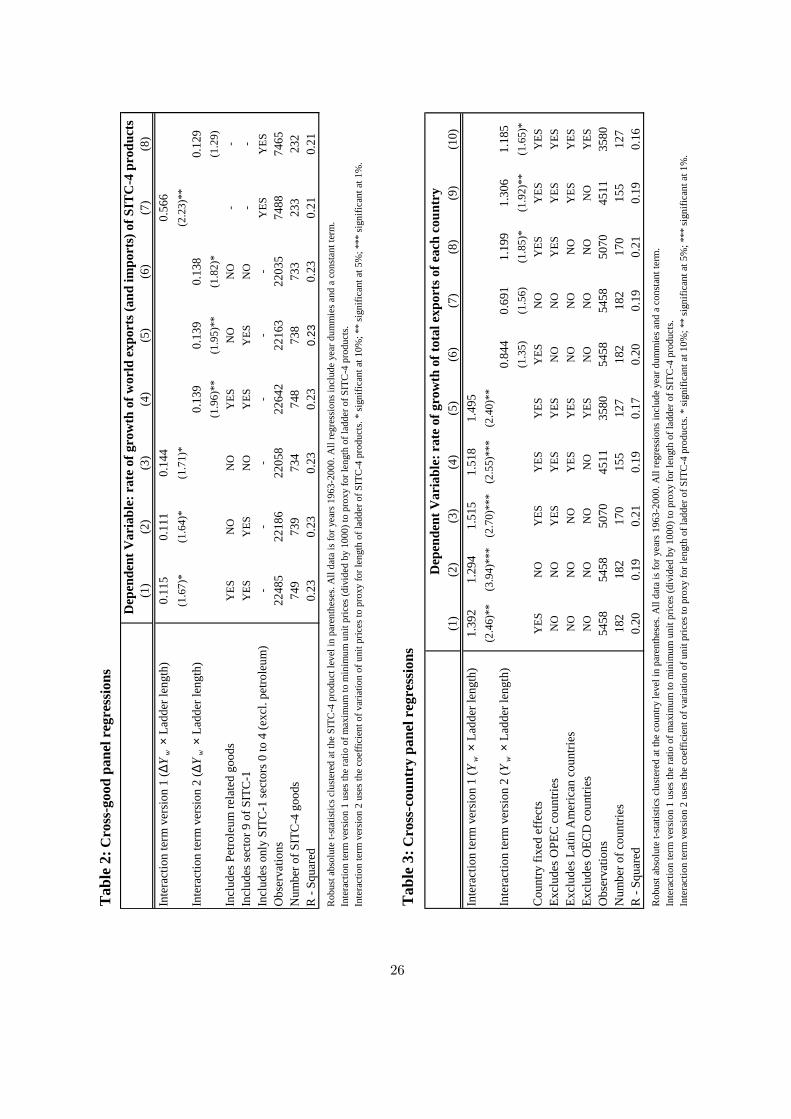
Table 2 displays the results of the cross-good regressions. The regressions using �interaction

term version 1�are run with the length of ladder being proxied by the max-to-min unit price

ratios. In the �rst column we use all the 4-digit goods. Column (2) removes petroleum related

goods (all goods coded 3300 through to 3400 in the dataset) in case these goods have a particular

in�uence on the results for reasons other than nonhomotheticity linked to heterogeneity in the

scope of quality di¤erentiation (for example, petroleum related goods may display relatively high

income demand elasticity not necessarily because they exhibit long quality ladders, but because

23

they may represent fundamental inputs in the production of long-ladder goods). Column (3)

removes all �ve goods in �Commodities and transactions not classi�ed elsewhere�as they seem

to be clear outliers according to Table 1. In the three cases, results are consistent with our

model�s prediction and all the estimates of � are signi�cantly di¤erent from zero at 10% level.

Similar conclusions (at somewhat higher signi�cance levels) follow from regressions in columns

(4)-(6), where the length of ladder is proxied by the coe¢ cients of variation of unit prices.20

Finally, in columns (7) and (8) we run regression (17) using only sectors producing primary

goods (excluding again petroleum related goods). Column (7) seems to suggest that the link

between scope of quality upgrading (proxied by the max-to-min price ratios) and income demand

elasticity is also present when we look only at primary goods; in (8) the coe¢ cient is also

positive although it fails to reach signi�cance at 10% level. This last result may suggest that our

mechanism might be relevant not only when comparing manufacturing versus agricultural goods,

as the Prebisch-Singer hypothesis has been traditionally presented in the North-South literature.

In particular, our model may also apply to cases in which the patterns of specialisation are not

strictly linked to di¤erent stages of economic development.21

5.3 Cross-Country Regressions

Our model also predicts that countries that specialise in the production of goods with longer

quality ladders should see their exports value increase more strongly when world income rises.

We assess this prediction resorting again to a reduced-form approach by conducting the following

regression:

�Xi;t = � + (�Yw;t � Ladderi;t) + �t + �i + �i;t; (18)

20Notice that since (17) is capturing a reduced-form correlation between the variables placed in the regression,

the product (� � Ladderj) cannot actually be interpreted as a component of the income demand elasticity ofgood j. More precisely, to estimate such elasticity we would �rst need to abstract from all general equilibrium

interactions that take place when international prices adjust to income shocks (in terms of our general equilibrium

model, we would need to remove the e¤ects brought about by the changes of w resulting from variations in �).

Nevertheless, our general equilibrium model still predicts a positive correlation between changes in the value of

exports of good j and its ladder�s length in a context of positive world income growth, which is the correlation

we aim to capture with (17).

21An illustrative example of how our model can be applied to rationalise patterns of specialisation of countries

at similar stages of economic development is presented next in Section 6, where we discuss the case of colonial

Jamaica and compare it to the one of pre-industrial Argentina.

24

where �Xi;t is the percentage growth of the total value of exports by country i in year t. The

variable Ladderi;t measures the average length of ladders of the bundle of goods exported by

i in year t: we build this variable by weighing Ladderj (i.e., the variable used before in our

cross-good regressions) of each good j by the share of that good in the total value of exports of

country i in period t. Our model thus predicts > 0.

Columns (1)-(5) in Table 3 show the results of di¤erent versions of (18) when we measure

the length of ladders by the max-to-min unit price ratios. Column (1) and (2) use all countries

in the panel, the former including country �xed e¤ects and the latter excluding them: in both

cases the estimates are positive, similar in magnitude, and highly signi�cant. In (3) we exclude

countries from the OPEC from the regression in case oil exporters may have a large impact on

the results (in particular, given that our sample includes years when the oil shocks occurred);

the previous results remain essentially intact. Results also remain unchanged when we exclude

Latin American economies from the sample in column (4) � in this case, the rationale is the

fact that many of these economies have gone through severe macroeconomic and external crises

during �80s and �90s, including large devaluations of their currencies. Finally, in (5) we exclude

the OECD countries to have some feeling about whether our results are crucially driven by

comparing developed economies to less developed ones; as we can readily observe, results still

remain essentially una¤ected when we restrict the sample in such a way.

In columns (6)-(10) we replicate the same regressions using the coe¢ cients of variation of

unit prices. Although the signi�cance of the estimates is lower than in (1)-(5), and in (6) and

(7) we fail to reach signi�cance at 10% level, all the estimates carry the expected sign and,

moreover, their magnitudes exhibit a similar pattern to those in (1)-(5).

Viewed from a longer run perspective, our model argues that, if countries� comparative

advantages across goods remain constant over time, the initial pattern of specialisation may

lead to uneven future exports growth when goods di¤er in their scope for quality upgrading.

Table 4 looks at how economies�initial specialisation correlates with future exports growth in

a context of positive world income growth. In particular, we are interested in investigating

whether, when focusing on periods of positive world income growth, countries that initially

specialise in goods with longer quality ladders will tend to experience a higher rate of growth of

their exports. For this purpose, we build a proxy for country i initial specialisation �in terms

of scope for (future) quality upgrading�by weighting the length of ladders of SITC-4 products

25

Tab

le 2

:Cro

ssg

ood

pane

l reg

ress

ions

(1)

(2)

(3)

(4)

(5)

(6)

(7)

(8)

Inte

ract

ion

term

ver

sion

1 ( Δ

Yw

× La

dder

leng

th)

0.11

50.

111

0.14

40.

566

(1.6

7)*

(1.6

4)*

(1.7

1)*

(2.2

3)**

Inte

ract

ion

term

ver

sion

2 ( Δ

Yw

× La

dder

leng

th)

0.13

90.

139

0.13

80.

129

(1.9

6)**

(1.9

5)**

(1.8

2)*

(1.2

9)In

clud

es P

etro

leum

rela

ted

good

sY

ESN

ON

OY

ESN

ON

O

In

clud

es se

ctor

9 o

f SIT

C1

YES

YES

NO

YES

YES

NO

Incl

udes

onl

y SI

TC1

sect

ors 0

to 4

(exc

l. pe

trole

um)

YES

YES

Obs

erva

tions

2248

522

186

2205

822

642

2216

322

035

7488

7465

Num

ber o

f SIT

C4

goo

ds74

973

973

474

873

873

323

323

2R

Sq

uare

d0.

230.

230.

230.

230.

230.

230.

210.

21R

obus

t abs

olut

e ts

tatis

tics c

luste

red

at th

e SI

TC4

pro

duct

leve

l in

pare

nthe

ses.

All

data

is fo

r yea

rs 1

963

2000

. All

regr

essi

ons i

nclu

de y

ear d

umm

ies a

nd a

con

stan

t ter

m.

Inte

ract

ion

term

ver

sion

1 u

ses t

he ra

tio o

f max

imum

to m

inim

um u

nit p

rices

(div

ided

by

1000

) to

prox

y fo

r len

gth

of la

dder

of S

ITC

4 p

rodu

cts.

Inte

ract

ion

term

ver

sion

2 u

ses t

he c

oeffi

cien

t of v

aria

tion

of u

nit p

rices

to p

roxy

for l

engt

h of

ladd

er o

f SIT

C4

pro

duct

s. *

sign

ifica

nt a

t 10%

; **

sign

ifica

nt a

t 5%

; ***

sign

ifica

nt a

t 1%

.

Dep

ende

nt V

aria

ble:

rat

e of

gro

wth

of w

orld

exp

orts

(and

impo

rts)

of S

ITC

4 p

rodu

cts

Tab

le 3

:Cro

ssc

ount

ry p

anel

reg

ress

ions

(1)

(2)

(3)

(4)

(5)

(6)

(7)

(8)

(9)

(10)

Inte

ract

ion

term

ver

sion

1 (Y

w×

Ladd

er le

ngth

)1.

392

1.29

41.

515

1.51

81.

495

(2.4

6)**

(3.9

4)**

*(2

.70)

***

(2.5

5)**

*(2

.40)

**In

tera

ctio

n te

rm v

ersi

on 2

(Yw

× La

dder

leng

th)

0.84

40.

691

1.19

91.

306

1.18

5(1

.35)

(1.5

6)(1

.85)

*(1

.92)

**(1

.65)

*C

ount

ry fi

xed

effe

cts

YES

NO

YES

YES

YES

YES

NO

YES

YES

YES

Excl

udes

OPE

C c

ount

ries

NO

NO

YES

YES

YES

NO

NO

YES

YES

YES

Excl

udes

Lat

in A

mer

ican

cou

ntrie

sN

ON

ON

OY

ESY

ESN

ON

ON

OY

ESY

ESEx

clud

es O

ECD

cou

ntrie

sN

ON

ON

ON

OY

ESN

ON

ON

ON

OY

ESO

bser

vatio

ns54

5854

5850

7045

1135

8054

5854

5850

7045

1135

80N

umbe

r of c

ount

ries

182

182

170

155

127

182

182

170

155

127

R

Squa

red

0.20

0.19

0.21

0.19

0.17

0.20

0.19

0.21

0.19

0.16

Rob

ust a

bsol

ute

tsta

tistic

s clu

ster

ed a

t the

cou

ntry

leve

l in

pare

nthe

ses.

All

data

is fo

r yea

rs 1

963

2000

. All

regr

essio

ns in

clud

e ye

ar d

umm

ies a

nd a

con

stan

t ter

m.

Inte

ract

ion

term

ver

sion

1 u

ses t

he ra

tio o

f max

imum

to m

inim

um u

nit p

rices

(div

ided

by

1000

) to

prox

y fo

r len

gth

of la

dder

of S

ITC

4 p

rodu

cts.

Inte

ract

ion

term

ver

sion

2 u

ses t

he c

oeffi

cien

t of v

aria

tion

of u

nit p

rices

to p

roxy

for l

engt

h of

ladd

er o

f SIT

C4

pro

duct

s. *

sign

ifica

nt a

t 10%

; **

sign

ifica

nt a

t 5%

; ***

sign

ifica

nt a

t 1%

.

Dep

ende

nt V

aria

ble:

rat

e of

gro

wth

of t

otal

exp

orts

of e

ach

coun

try

26

Table 4: Future exports growth regressions

(1) (2) (3) (4) (5) (6) (7) (8)

Initial ladder length (196266) version 1 3.91 4.58 5.22 5.21( 2.48)** (2.70)*** (2.50)** (2.42)**

Initial ladder length (196266) version 2 1.40 2.87 2.80 2.50(1.18) (2.36)** (2.22)** (2.05)**

Excludes OPEC countries NO YES YES YES NO YES YES YESExcludes Latin American countries NO NO YES YES NO NO YES YESExcludes OECD countries NO NO NO YES NO NO NO YESObservations 140 129 114 89 140 129 114 89R Squared 0.04 0.06 0.07 0.07 0.01 0.04 0.04 0.03

Initial ladder length version 1 uses the maxtomin unit price ratios (divided by 1000) to proxy for length of ladder of SITC4 products, weightingthese ratios by the average exports shares of each product during years 196266. Initial ladder length version 2 uses the coeffients of variation of unit prices.Dependent variable is the average growth of total exports by each country during years in the sample in which world income per head displays positive growth.Robust tstatistics in parentheses. All regressions include a constant term. * significant at 10%; ** significant at 5%; *** significant at 1%.

Average growth of exports using years of positive world income growthSample: years 19712000

by their average export shares during years 1962-66. Notice that, although we use the �rst �ve

years in the sample for the export-share weights, the length of ladders for each SITC-4 good are

still being proxied by the max-to-min price during the last year in the sample (i.e. year 2000).

This is in line with the logic of our model, where goods�potential of quality upgrading is the

feature that really matters for long-run exports growth, and the process of quality upgrading

itself materialises over time as world productivity expands and world income rises accordingly.

In Table 4 we take the subsample of years in the period 1971-2000, and we compute the

average growth of exports of each country, using only years in which world income per head

growth was positive. Next, we regress those average growth rates on countries�initial length of

ladder, which are built as explained in the above paragraph. As for Table 3, we run regressions

including all countries in the sample, and subsequently excluding OPEC, Latin American and

OECD countries, in that order. All the regressions (except for column 5) reach the same conclu-

sion: the patterns of specialisation during the �rst �ve years in the sample (in terms of average

length of ladders of exports during 1962-66) correlates signi�cantly with the average growth of

future exports during years of positive world income growth. (We ran the same regressions using

the subsample 1981-2000; the results obtained are qualitatively similar to those in Table 4 and

are available from the authors upon request.)22

22All regressions in Table 3 and Table 4 include sector 9 of the 1-digit SITC categorisation. Results obtained

excluding goods in sector 9 are very similar to those presented before, and are available upon request.

27

6 An Illustrative Historical Example: colonial Jamaica and

pre-industrial Argentina

Situations where the mechanism proposed in this paper may have played an important role

include the cases of economies for which exogenous initial geographical conditions greatly in�u-

enced their specialisation in the world economy during some period in history. As an illustrative

example, we take the case of colonial Jamaica (denoted by J) and compare it to the one of

pre-industrial Argentina (denoted by A). In this example, we consider two goods, namely sugar

(denoted by s) and beef (denoted by b).

From the second half of the XVII century until the �rst half of the XIX century, the Jamaican

economy grew mainly based on the production and export of sugar from sugarcane. This is not

surprising given the excellent climatic conditions this tropical island o¤ered for that type of crop.

By 1805, Jamaica was the largest sugar exporter in the world (Higman, 2005). Given the value

attributed to sugar by European consumers, during that period Jamaica was deemed probably

the most important British colony in the Americas (Hall, 1959; Sheridan, 1973). Although sugar

was indeed a very valuable consumption good at that time, it clearly was a type of good with

very limited scope for undergoing subsequent improvements in quality. As such, according to

our model, sugar was bound to eventually lose its status of luxury among consumers as their

incomes would rise.23 In fact, by the second half of the XIX century, sugar began to lose its

economic preeminence in the world markets and started experiencing a long phase of declining

(relative) prices, which in turn seriously damaged the Jamaican economy.24

In Argentina, geographical conditions made this country exceptionally apt for the breeding

of cattle and growing cereals, which constituted the main engines of its economy until 1914.

The commercial production of cattle started in the late second half of the XVIII century with

the appearance of the saladeros �slaughterhouses where meat would be cured by drying and

salting (Newton, 1966). Salt-cured beef was a rather unsophisticated product that was mostly

23 In that regard, Sheridan (1973) writes, "Until the late years of the 17th century English sugar consumption

seems to have been con�ned rather closely to the wealthy sections of society. [...] Lower income groups were

reported to have used quantities of molasses, treacle and low-quality sugar to sweeten their eatables, and to make

drinkable liquors. [...] During the 18th century the [physical ] demand for sugar grew so rapidly among all sections

of English society that few people considered it a luxury [anymore ]."24By 1820 the GDP per head in Jamaica was 1.05 times the world average GDP per head, whereas by 1870 it

equalled 0.61 the world average GDP per head. In fact, during the period 1820-1870, income per head in Jamaica

fell 23.6%, while the world average income per head grew 31%. Data taken from Maddison (2008).

28

exported to Cuba and Brazil to feed slaves. In fact, the industry of the saladeros did not mean

a big push to the Argentinean economy, which was at that time still a very marginal country

within the world economy.

The big boom for the cattle industry in Argentina came much later, at the end of the XIX

century. Unlike the sugar industry, the cattle industry had some scope for quality upgrad-

ing, in the form of chilled and frozen beef. The market size for this product, certainly more

appreciated by consumers than salt-cured beef, was however initially quite limited, since the

transportation cost induced a huge di¤erential in the prices of the two goods. Yet, in Europe,

incomes had been continuously rising during the XIX century, thanks to the massive technolog-

ical advancement that followed the advent of the Industrial Revolution. The availability of a

higher-quality commodity in the cattle industry eventually attracted well-to-do European con-

sumers, whose demand induced Argentinean �rms to export large amounts of chilled and frozen

beef to Europe.25 During the period 1890-1914, Argentina grew on average at rate of 5.5%

yearly, attracted millions of immigrants from Europe and became one of the richest countries in

the world (Maddison, 2008).26 The exportation of chilled and frozen beef was undoubtedly one

of the main activities that spurred this phase of fast and steady economic growth in Argentina

between 1880-1914 (Rapaport, 1988).

This example illustrates how exogenous geographical conditions greatly in�uenced the path of

GDP growth in Jamaica and in Argentina via the evolution of their exports, in the way our model

would predict. Jamaica was comparatively e¢ cient at producing sugar, while Argentina enjoyed

a comparative advantage in beef production (in terms or our model, aJs < aAs and aAb < aJb ).

Sugar o¤ered very limited scope for quality improvements, which is analogous to assuming that

the cost of quality upgrading for sugar products is extremely high. On the contrary, beef did

o¤er some more scope for quality upgrading than sugar (in our model, �b < �s). The latter

materialised in the switch from salt-cured beef production (lower-quality commodity) to chilled

and frozen beef (higher-quality commodity). As predicted by our model, sugar exports initially

sustained high growth in Jamaica, until rising income in the world (i.e., driven by rising �)

shifted aggregate world expenditure towards goods which could be o¤ered in higher quality

25The main market for Argentinean chilled and frozen beef at that time was by far the prosperous Great

Britain of end of XIX and beginning of XX century (in 1914, 83.5% of the total Argentinean exports of chilled

and frozen beef was sent to the UK). See Rapaport (1988).

26By 1913, the GDP per head in Argentina was slightly larger than that of France and Germany, and it was

0.77 times the GDP per head in the UK. Data taken from Maddison (2008).

29

degrees, such as chilled and frozen beef from Argentina.27

7 Conclusion

We have proposed a model of international trade with nonhomothetic preferences based on

comparative advantages that are unrelated to the stage in the process of development in which

countries are. This feature represents the main point of departure with respect to the past

literature on North-South trade, where the comparative advantage stems from the fact that

some countries (the North) have historically accumulated larger amounts of capital than others

(the South).

The key novel �nding of our model is pointing out that even when no single country enjoys

a clear absolute advantage over any other country and productivity changes are uniform and

identical in all countries, international trade may still be the source of income divergence in

the world economy when nonhomothetic preferences and quality ladders are jointly taken into

account. In particular, countries� incomes will diverge when comparative advantage induce

patterns of specialisation that, although optimal for each country at early stages in the process

of development, do not o¤er the same scope for improvements in terms of quality upgrading of

�nal products in the long run.

Our model also points out that worldwide uniform productivity growth generates two dis-

tinct types of product cycle phenomena. The �rst is an international product cycle phenomenon

à la Linder-Vernon, where over time one economy takes on the production of goods previously

produced by another economy. The second �which is novel to our model �is a regional prod-

uct cycle that occurs within each good and within each economy: rising world income makes

all economies engage in the production of newer goods of higher quality (so as to satisfy the

increasing demand for high qualities by wealthier consumers).

Admittedly, we have presented a largely stylised model, simpli�ed in several dimensions, so

as to illustrate in a concise way our main mechanism and its implications: the fact that the dy-

27One may argue that the productivity improvement discussed in the illustrative example should be read as

a rise in good-speci�c productivity (in our model, a fall in ab) rather than an increase in aggregate productivity.

Even if we supposed that was the case, a mere change in this parameter would not necessarily rationalise the

facts illustrated in this example, as the way total expenditure shares in good b would respond to a change in ab

crucially depends on the price elasticity of beef demand. Therefore, variations in ab would not necessarily a¤ect

the relative terms of trade between the two countries in such a way as to account for the increase in per-capita

Argentinean income relative to Jamaican observed in historical data.

30

namics of quality upgrading in consumption, in a context of worldwide growth and international

trade, may cause world demand to continuously shift towards those economies that produce

commodities o¤ering larger scope for quality improvements. This result may hold, nonetheless,

under more general assumptions regarding preferences and technology, some of them already

discussed in previous sections.

Concerning preferences, the essential feature is that the marginal utility of quality upgrading

rises with income fast enough relative to the marginal cost of quality upgrading. With respect

to the technology itself, somewhat restrictive assumptions such as: (i) the monotonicity of A(v)

in Assumption 1 or (ii) the fact that functions a(v) and a�(v) are both increasing in v, could

be relaxed. A non-monotonic A(v) will certainly lead to richer general equilibrium responses

to worldwide technological growth. Yet, the key �nding that the economy specialising in the

goods with lowest cost of quality upgrading will eventually experience faster growth through the

improvement of its terms of trade would still obtain. On the other hand, letting a(v) and a�(v)

behave in an unrestricted way may give rise to changes and switches in the order of quality

upgrading across goods. However, again, the goods with relatively low elasticity of quality

upgrading, i.e. those with relatively low �(v), will eventually become those that experience

relatively fast quality upgrading, just as it occurred in our benchmark model.

We conducted a number of empirical exercises which suggest that the central theoretical

predictions of our model �nd some empirical support in the trade data. In particular, we �nd

that exports, both at a world- and country-level of aggregation, correlate with world income

changes in a way that is consistent with our theory. Our tests followed two stylised reduced-

form approaches. The �rst approach shows that long-ladder goods tend to attract increasing

world expenditure shares with rising world income. The second approach shows that exports

from countries specialising in the production of long-ladder goods increase relatively more when

world income rises. In addition, our �nding that economies�initial specialisation correlates with

future exports growth in a context of world income growth is suggestive of the fact that initial

comparative advantage may lead to uneven future exports growth when goods di¤er in their

scope for quality upgrading.

Finally, here, we have focused on illustrating how our theory may shed light on historical

cases where comparative advantage emerged exogenously, for example as a result of geographical

conditions. Other issues, including what determines the relative successes of economies with

similar comparative advantage, and why richer countries tend to trade among themselves more

than they do with poorer economies, are the subject of ongoing research.

31

Appendices

A First-Order Conditions for Consumption Choice in H

The optimisation problem in (5) yields the following �rst-order conditions (where � represents

the Lagrange multiplier associated to the budget constraint and f�vgv2V denote those associatedto the constraints fqv � 1gv2V):

ln

�vw

��1� (v) q�(v)v

!� � (v) + �v = 0; 8v 2 V; (19)

qv�v� � = 0; 8v 2 V; (20)

qv � 1 � 0; �v � 0; and �v (qv � 1) = 0; 8v 2 V; (21)

1�ZV�v dv = 0: (22)

From (20), it follows that �v = qv=�. Then, replacing this last expression into (22) leads toRV qz dz = �, from where the condition (6) immediately obtains by using again (20).

By using the condition (6), we can rewrite (19) as:

�v = � (v) + ln [� (v) =w]� ln�+ lnQ+ [� (v)� 1] ln qv: (23)

The expression in (23) will be used in many of the following proofs.

B Optimal Consumption Choice in F

Bearing in mind Assumption 1, we can write down the optimisation problem faced by a repre-

sentative individual from F as follows:

maxfx�vqg(v;q)2V�Q

U� =

ZVq�v ln

�w��vpv

�dv;

subject to:RV �

�vdv = 1;

q�v � 1; 8v 2 V;

pvq = ��1q�(v)� (v) ; 8 (v; q) 2 V�Q:

Lemma 4 holds for x�vq in a similar fashion as for xvq. Hence, we can re-state the problem

speci�ed above in terms of q�v and ��v, as it was previously done for H (where q�v now denotes

32

the quality of good v consumed, in the optimum, in F). This way, we can obtain the following

�rst-order conditions, which constitute the analogous versions for F of (6) and (23), respectively:

��v =q�vR

V q�z dz

; 8v 2 V; (24)

��v = � (v) + ln [� (v) =w�]� ln�+ lnQ� + [� (v)� 1] ln q�v : (25)

Given the �rst-order conditions in (24) and (25), all the ensuing results found in Section 3 fol-

low through in qualitative terms. In particular, we can derive functions fq�vgv2V and f��vgv2V dis-playing identical qualitative properties as their counterparts in H, that is fqvgv2V and f�vgv2V,in terms of Lemmas 1 - 2 and Proposition 1. Furthermore, we can similarly �nd the thresh-

old �� for the worldwide aggregate-productivity parameter, which splits F in the regimes of

subsistence-economy and modern-economy ; both exhibiting analogous properties as described

for H.28 Finally, likewise for H in Corollary 1, for F the following holds:

Corollary 2

Let #� (v) �R v0 �

�z dz. Then:

(i) 8� 2 (0; ��) ) @#� (v) =@� = 0, 8 v 2 V;(ii) 8� � �� ) @#� (v) =@� > 0; 8v 2 V; with strict inequality if v < 1.

C Omitted Proofs

Proof of Lemma 1.

Suppose qv < qv. Since by de�nition qv � 1, then qv > 1, hence (23) paired with (21) yield:

� (v) + ln [� (v) =w]� ln (�=Q) � 0;

while:

� (v) + ln [� (v) =w]� ln (�=Q) + [� (v)� 1] ln qv = 0:

Thus:

� (v) + ln� (v) � � (v) + ln� (v) + [� (v)� 1] ln qv:

This last equality in turn leads to:

[� (v)� � (v)] + ln [� (v) =� (v)] + [� (v)� 1] ln qv � 0;

28From Section 4, it is straightforward to observe that, given Assumption 1, �� = �.

33

which cannot possibly hold if qv > 1, as its left-hand side would then be strictly positive.

Therefore, it must necessarily be the case that qv � qv.

Suppose now qv = qv > 1. In this case, (23) in conjunction with (21) yield:

� (v) + ln� (v) + [� (v)� 1] ln qv = � (v) + ln� (v) + [� (v)� 1] ln qv = 0:

This last equality in turn leads to:

� [� (v)� � (v)] (1 + ln qv) = ln [� (v) =� (v)] :

However, this last equality cannot possibly hold since its right-hand side is strictly positive,

while the left-hand side is negative. As a result, qv > qv must necessarily hold when qv > 1.

Proof of Lemma 2.

Part (i). Proof follows immediately from noting that Lemma ?? implies that, whenever � 2(0; �), qv = 1 must hold for all v 2 V. Thus, whenever � 2 (0; �), @qv=@� = 0 for all v 2 V.

Part (ii). Firstly, notice that, since qv = 1 must hold for all v =2 L, a proof analogous to

that of Part (i) of this Lemma applies for all goods in this subset. Secondly, for any v 2 L,di¤erentiating (31) with respect to � yields:

dqvd�

=� (0)� 1� (v)� 1

"e�(0)� (0)

e�(v)� (v)

# 1�(v)�1

(q0)�(0)��(v)�(v)�1

dq0d�; 8v 2 L:

Using again (31), the equation above can be written:

dqvd�

=� (0)� 1� (v)� 1

qvq0

dq0d�; 8v 2 L: (26)

(Since � (�) > 1, notice that dqv=d� and dq0=d� must then share the same sign, for all v 2 L).Given that:

Q = 1� ~v(�) +Z ~v(�)

0qz dz;

it follows that:dQ

d�=

Z ~v(�)

0

dqzd�dz =

1

q0

Z ~v(�)

0

� (0)� 1� (z)� 1qzdz

!dq0d�:

Applying (23) to v = 0 when �0 = 0 yields: q0 =�a (0) e�(0)Q

�� 1�(0)�1 �

1�(0)�1 . Thus:

dq0d�

=q0

� (0)� 1Q

�

1� ~v +

Z ~v(�)

0

� (z)

� (z)� 1 qz dz!�1

> 0:

34

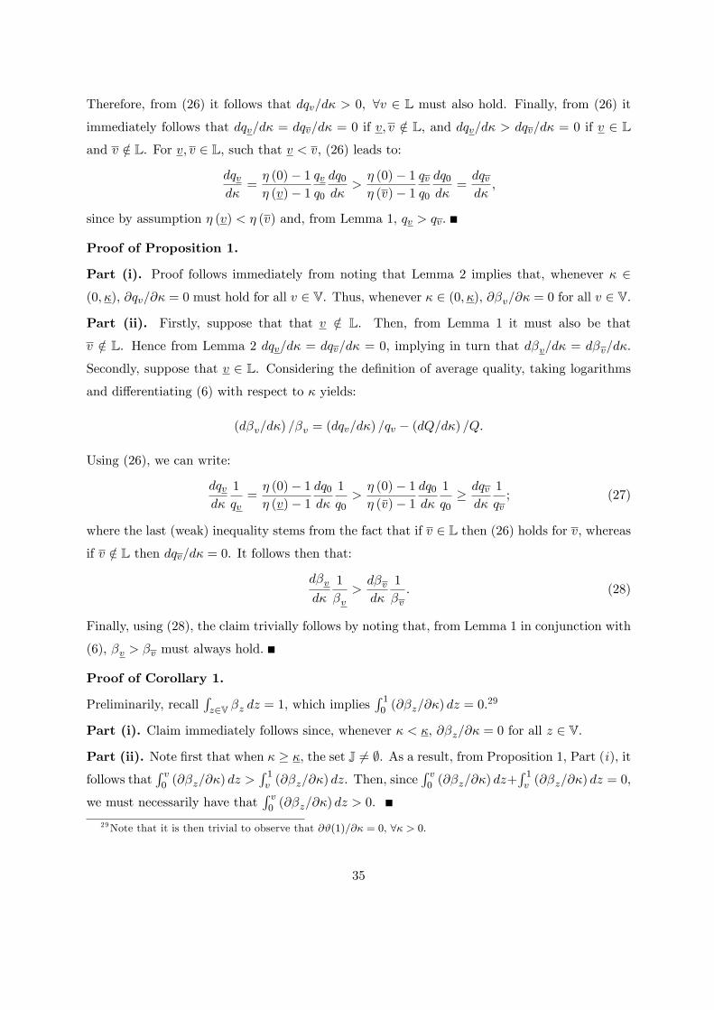
Therefore, from (26) it follows that dqv=d� > 0; 8v 2 L must also hold. Finally, from (26) it

immediately follows that dqv=d� = dqv=d� = 0 if v; v =2 L, and dqv=d� > dqv=d� = 0 if v 2 Land v =2 L. For v; v 2 L, such that v < v, (26) leads to:

dqvd�

=� (0)� 1� (v)� 1

qvq0

dq0d�

>� (0)� 1� (v)� 1

qvq0

dq0d�

=dqvd�;

since by assumption � (v) < � (v) and, from Lemma 1, qv > qv.

Proof of Proposition 1.

Part (i). Proof follows immediately from noting that Lemma 2 implies that, whenever � 2(0; �), @qv=@� = 0 must hold for all v 2 V. Thus, whenever � 2 (0; �), @�v=@� = 0 for all v 2 V.

Part (ii). Firstly, suppose that that v =2 L. Then, from Lemma 1 it must also be that

v =2 L. Hence from Lemma 2 dqv=d� = dqv=d� = 0, implying in turn that d�v=d� = d�v=d�.

Secondly, suppose that v 2 L. Considering the de�nition of average quality, taking logarithmsand di¤erentiating (6) with respect to � yields:

(d�v=d�) =�v = (dqv=d�) =qv � (dQ=d�) =Q:

Using (26), we can write:

dqvd�

1

qv=� (0)� 1� (v)� 1

dq0d�

1

q0>� (0)� 1� (�v)� 1

dq0d�

1

q0� dqvd�

1

qv; (27)

where the last (weak) inequality stems from the fact that if v 2 L then (26) holds for v, whereasif v =2 L then dqv=d� = 0. It follows then that:

d�vd�

1

�v>d�vd�

1

�v: (28)

Finally, using (28), the claim trivially follows by noting that, from Lemma 1 in conjunction with

(6), �v > �v must always hold.

Proof of Corollary 1.

Preliminarily, recallRz2V �z dz = 1, which implies

R 10 (@�z=@�) dz = 0:

29

Part (i). Claim immediately follows since, whenever � < �; @�z=@� = 0 for all z 2 V.

Part (ii). Note �rst that when � � �, the set J 6= ;. As a result, from Proposition 1, Part (i), itfollows that

R v0 (@�z=@�) dz >

R 1v (@�z=@�) dz. Then, since

R v0 (@�z=@�) dz+

R 1v (@�z=@�) dz = 0,

we must necessarily have thatR v0 (@�z=@�) dz > 0.

29Note that it is then trivial to observe that @#(1)=@� = 0, 8� > 0.

35

D Auxiliary Derivations and Proofs

Lemma 3

Let � � a (0) exp [� (0)]. Then:

(i) 8� 2 (0; �) ) L = ;;

(ii) 8� � � ) L = [0; ~v(�)] ; where ~v(�) : [�;1) ! [0; 1] ; ~v(�) = 0; ~v0 (�) � 0, with strict

inequality if ~v (�) < 1.

Proof.

Part (i). When � 2 (0; �), conditions stipulated in (21) and (23) applied on v = 0 entail that:q0 = 1 and �0 > 0. As a result, from Lemma 1 it follows that qv = 1, 8v 2 V: Therefore, sincea0 (v) � 0 and �0 (v) > 0, again from (23), �v > 0 for all v 2 V obtains, and thus L = ;.

Part (ii). Firstly, note that (23) applied on v = 0, in conjunction Lemma 1, implies that when

� = �, then �0 = 0 and q0 = 1. Then, Lemma 1 implies Q = 1. Using these results in (23)

yields:

�v = � (v) + ln [� (v) =w]� ln�;

implying that �v > 0 for all v 2 (0; 1]. As a result, the set L = ;, meaning that ~v(�) = 0.

Secondly, notice that, from Lemma 4 below, @�0;v (v) =@v < 0 and @�0;v (v) =@v < 0 since

a0 (v) � 0 and �0 (v) > 0, hence the set L � V comprises the lower-indexed goods in V, with

~v(�) representing its upper bound. Given Lemma 1 and Lemma 5 below, the aggregate quality

index can be written as follows:

Q = 1� ~v(�) +Z ~v(�)

0qv dv:

Furthermore, observe that, whenever ~v(�) < 1:

ln (�=Q) = � (~v(�)) + ln [� (~v(�)) =w]

must hold in equilibrium. This last condition yields, after some simple algebra:

Q = �w exp [�� (~v)] =� (~v) :

In addition to that, because of Lemma 1, in equilibrium:

[� (v)� 1] ln qv = ln (�=Q)� � (v)� ln [� (v) =w]

36

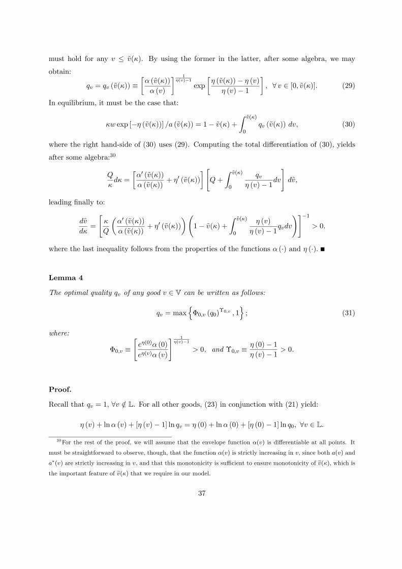
must hold for any v � ~v(�). By using the former in the latter, after some algebra, we may

obtain:

qv = qv (~v(�)) �� (~v(�))

� (v)

� 1�(v)�1

exp

�� (~v(�))� � (v)� (v)� 1

�, 8 v 2 [0; ~v(�)]: (29)

In equilibrium, it must be the case that:

�w exp [�� (~v(�))] =a (~v(�)) = 1� ~v(�) +Z ~v(�)

0qv (~v(�)) dv; (30)

where the right hand-side of (30) uses (29). Computing the total di¤erentiation of (30), yields

after some algebra:30

Q

�d� =

��0 (~v(�))

� (~v(�))+ �0 (~v(�))

�"Q+

Z ~v(�)

0

qv� (v)� 1dv

#d~v;

leading �nally to:

d~v

d�=

"�

Q

��0 (~v(�))

� (~v(�))+ �0 (~v(�))

� 1� ~v(�) +

Z ~v(�)

0

� (v)

� (v)� 1qvdv!#�1

> 0:

where the last inequality follows from the properties of the functions � (�) and � (�).

Lemma 4

The optimal quality qv of any good v 2 V can be written as follows:

qv = maxn�0;v (q0)

�0;v ; 1o; (31)

where:

�0;v �"e�(0)� (0)

e�(v)� (v)

# 1�(v)�1

> 0, and �0;v �� (0)� 1� (v)� 1 > 0.

Proof.

Recall that qv = 1, 8v =2 L. For all other goods, (23) in conjunction with (21) yield:

� (v) + ln� (v) + [� (v)� 1] ln qv = � (0) + ln� (0) + [� (0)� 1] ln q0; 8v 2 L:

30For the rest of the proof, we will assume that the envelope function �(v) is di¤erentiable at all points. It

must be straightforward to observe, though, that the function �(v) is strictly increasing in v, since both a(v) and

a�(v) are strictly increasing in v, and that this monotonicity is su¢ cient to ensure monotonicity of ev(�), which isthe important feature of ev(�) that we require in our model.

37

Isolating [� (v)� 1] ln qv, and applying exponentials to both sides gives:

(qv)�(v)�1 =

e�(0)

e�(v)�(0)

� (v)(q0)

�(0)�1 ; 8v 2 L:

Finally, raising both sides to the power [� (v)� 1]�1, and considering Lemma 1, (31) obtains.

Lemma 5

If ~v(�) < 1, then q~v(�) = 1.

Proof.

By de�nition of L, �~v(�) = 0. Thus, the condition (23) applied on ~v(�) yields:

� (~v(�)) + ln [� (~v(�)) =w]� ln�+ lnQ = � [� (~v(�))� 1] ln q~v(�) (32)

Suppose now that q~v(�) > 1, and take some " 2 (0; 1 � ~v(�)]. Then, since v = ~v(�) + " =2 L, itmust be the case that:

� (~v(�) + ") + ln [� (~v(�) + ") =w]� ln�+ lnQ = �~v(�)+": (33)

Then, by continuity of � (�) and � (�), and using the result in (32), we must have:

lim"!0

f� (~v(�) + ") + ln [� (~v(�) + ") =w]� ln�+ lnQg = � [� (~v(�))� 1] ln q~v(�) < 0:

Hence, q~v(�) > 1 cannot possibly hold when ~v(�) < 1 as it would imply that �~v(�)+" < 0 in (33)

for "! 0, violating (21).

Proof of @#(m)=@w � 0.

Suppose �rst that ~v < m. Then, L � [0;m). Di¤erentiating (23) with respect to w yields:

� (v)� 1qv

@qv@w

+1

Q

@Q

@w= 0; 8v 2 L: (34)

Furthermore, from (31) it follows that:

@qv@w

=� (0)� 1� (v)� 1

qvq0

@q0@w

; 8v 2 L: (35)

Since @Q=@w =R ~v0 (@qz=@w) dz, combining (34) and (35) yields:�1� ~v +

Z ~v

0

� (z)

� (z)� 1qzdz�� (0)� 1q0

1

Q

@q0@w

= 0 ) @q0@w

= 0;

38

Therefore, using again (35), @qv=@w = 0 for all v 2 [0; ~v] obtains. In addition, because of Lemma1, it must thus be the case that @qv=@w = 0 holds as well for all v 2 (~v; 1]. Finally, recalling (6)it then follows that @�v=@w = 0 for all v 2 V, which in turn implies that @# (m) =@w = 0.Suppose now that ~v � m. Di¤erentiating (23) with respect to w now yields:

� (v)� 1qv

@qv@w

+1

Q

@Q

@w=

8<: 0; 8v 2 [0;m)1=w; 8v 2 [m; ~v]

(36)

From (36) it follows that a necessary condition for @# (m) =@w > 0 to hold is that @Q=@w < 0.31

However, (36) means that if @Q=@w < 0, then @qv=@w > 0 should hold for all v 2 [m; ~v]. If~v = 1; it must be straightforward to observe that @Q=@w < 0 cannot thus hold. Alternatively, if

~v < 1, then @Q=@w < 0 would require that @qv=@w < 0 prevails for some v 2 (~v; 1] which is notfeasible either since it would lead to violating the constraint qv � 1. As a result, @Q=@w � 0

must hold, which in turn implies @# (m) =@w � 0.

Proof of @#� (m) =@w < 0.

Suppose �rst that ~v� < m. Then, L�� [0;m). Di¤erentiating (23) �adjusted for representingan individual from F �with respect to w yields:

� (v)� 1q�v

@q�v@w

+1

Q�@Q�

@w= � 1

w; 8v 2 L�: (37)

In addition, from (31) it follows that:

@q�v@w

=� (0)� 1� (v)� 1

q�vq�0

@q�0@w

; 8v 2 L�: (38)

Combining (37) and (38) leads to: 1� ~v� +

Z ~v�

0

� (z)

� (z)� 1qzdz!� (0)� 1q�0

1

Q�@q�0@w

= � 1w

) @q�0@w

< 0:

Hence, using again (38), @q�v=@w < 0 for all v 2 [0; ~v�] obtains, which in turn implies @Q�=@w <0. Next, since for all v � ~v� the constraint q�v � 1 is binding, it must be the case that @q�v=@w � 0,8v 2 (~v�; 1]. As a result, because of (6), @��v=@w > 0 for all v 2 [m; 1] follows, which in turnimplies @#� (m) =@w < 0.

Suppose now ~v� � m. Di¤erentiating (23) with respect to w now yields:

� (v)� 1q�v

@q�v@w

+1

Q�@Q�

@w=

8<: �1=w; 8v 2 [0;m)0; 8v 2 [m; ~v�]

(39)

31Otherwise, if @Q=@w � 0, (36) would imply that @qv=@w � 0 for all v 2 [0;m). Recalling (6), it is thenstraightforward to observe that @Q=@w � 0 would mean @�v=@w � 0 for all v 2 [0;m), which in turn leads to@# (m) =@m � 0.

39

Suppose @Q�=@w � 0. From (39) it follows that @q�v=@w < 0 for all v 2 [0; ~v�). Furthermore,Lemma 1 then implies that @q�v=@w � 0 for all v 2 [~v�; 1]; as a result, @Q�=@w < 0 must

necessarily hold. Now, notice that if @Q�=@w < 0, then (39) implies @q�v=@w > 0 for all v 2[m; ~v�]. Moreover, in case ~v� < 1, since 8v 2 (~v�; 1] the constraint q�v � 1 is binding, @q�v=@w � 0must necessarily hold for all v 2 (~v�; 1]. As a result, if @Q�=@w < 0, then @��v=@w > 0 for allv 2 [m; 1], which in turn leads to @#� (m) =@w < 0.

References

[1] Alcala, F. (2009). �Comparative advantage across goods and product quality�, DT02/09, BBVA

Foundation.

[2] Benedetti Fasil, C. and Borota, T. (2009). �World Trade Patterns and Prices: The Role of Produc-

tivity and Quality Heterogeneity�, Mimeo, Uppsala University.

[3] Bertola, G., Foellmi, R. and Zweimuller, J. (2006). Income distribution in macroeconomic models,

Princeton: Princeton University Press.

[4] Brooks, E. (2006). �Why don�t �rms export more? Product quality and Colombian plants�, Journal

of Development Economics, vol. 80, pp. 160-178.

[5] Dornbusch, R., Fischer, S. and Samuelson, P. (1977). �Comparative advantage, trade, and payments

in a ricardian model with a continuum of goods�, American Economic Review, vol. 67, pp. 823-839.

[6] Fajgelbaum, P., Grossman, G. and Helpman, E. (2009). �Income distribution, product quality, and

international trade�, Mimeo, Harvard University.

[7] Feenstra, R. C., Lipsey, R. E., Deng, H., Ma, A. C. and Mo, H. (2005) �World Trade Flows: 1962-

2000�, NBER Working Paper No. W11040.

[8] Fieler, A. C. (2007). �Quality Di¤erentiation in International Trade: Evidence from the Demand

and Supply Sides�, Mimeo, NYU.

[9] Flam, H. and Helpman, E. (1987). �Vertical product di¤erentiation and North-South trade�, Amer-

ican Economic Review, vol. 77, pp. 810-822.

[10] Foellmi, R., Hepenstrick, C. and Zweimuller, J. (2008). �Income e¤ects in the theory of monopolistic

competition and international trade�, Mimeo, University of Zurich.

40

[11] Grossman, G. and Helpman, E. (1991). �Quality ladders and product cycles�, Quarterly Journal of

Economics, vol. 106, pp. 557-586.

[12] Hall, D. (1959). Free Jamaica, 1838-1865: an economic history, New Haven: Yale University Press.

[13] Hallak, J. C. (2006). �Product quality and the direction of trade�, Journal of International Eco-

nomics, vol. 68, pp. 238-265.

[14] Hallak, J. C., and Schott, P. (2009). �Estimating cross-country di¤erences in product quality�, Mimeo.

[15] Higman, B. W. (2005). Plantation Jamaica, 1750-1850: capital and control in a colonial economy,

Jamaica: University of the West Indies Press.

[16] Horvath, M. (2000). �Sectoral shocks and aggregate �uctuations�, Journal of Monetary Economics,

vol. 45, pp. 69-106.

[17] Iacovone, L. and Javorcik, B. (2008). �Shipping good tequila out: Investment, domestic unit values

and entry of multi-product plants into export markets�, Mimeo, Oxford University.

[18] Khandelwal, A. (2009). �The long and short (of) quality ladders�, Review of Economic Studies,

forthcoming.

[19] Lewbel, A. (2006). Engel Curves. The New Palgrave Dictionary in Economics, 2nd Edition.

[20] Linder, S. (1961). An essay on trade and transformation, Uppsala: Almqvist & Wiksell.

[21] Maddison, A. (2008). Statistics on World Population, GDP and Per Capita GDP, 1-2006 AD.

Website: http://www.ggdc.net/maddison.

[22] Matsuyama, K. (2000). �A Ricardian model with a continuum of goods under nonhomothetic prefer-

ences: demand complementarities, income distribution, and North-South trade�, Journal of Political

Economy, vol. 108, pp. 1093-1120.

[23] Newton, J. (1966). Historia de la sociedad rural argentina, Buenos Aires: Editorial Goncurt

[24] Prebisch, R. (1950). The economic development of Latin America and its principal problems. United

Nations, Econ. Comm. Latin America.

[25] Rapaport, M. (1988). Economia e historia: contribuciones a la historia economica argentina, Buenos

Aires: Libreria Editorial Tesis.

41

[26] Sheridan, R. (1973). Sugar and slavery: an economic history of the British West Indies 1623-1775,

Baltimore: The John Hopkins University Press.

[27] Schott, P. (2004). �Across-product versus within-product specialization in international trade�, Quar-

terly Journal of Economics, vol. 119, pp.647-678.

[28] Singer, H. (1950). �The distributions of gains between investing and borrowing countries�, American

Economic Review, vol. 40, pp. 473-485.

[29] Stokey, N. (1991). �The volume and composition of trade between rich and poor countries�, Review

of Economic Studies, vol. 58, pp. 63-80.

[30] Taylor, M. S. (1993). �Quality ladders and Ricardian trade�, Journal of International Economics,

vol. 34, pp. 225-243.

[31] Verhoogen, E. (2008). �Trade, Quality Upgrading andWage Inequality in the Mexican Manufacturing

Sector�, Quarterly Journal of Economics, vol. 123, pp 489-530.

[32] Vernon, R. (1966). �International investment and international trade in the product cycle�, Quarterly

Journal of Economics, vol. 80, pp 190-207.

42

quality ladders in a ricardian model of trade with

Documents