A Model of Trade with Ricardian Comparative Advantage and

Intra-sectoral Firm Heterogeneity�

Haichao FANy Edwin L.-C. LAIz Han (Ste¤an) QIx

October 3, 2013

Abstract

In this paper, we incorporate Ricardian comparative advantage into a multi-sector version of

Melitz�s (2003) model to explain the pattern of international specialization and trade. The model

is able to capture the existence of inter-industry trade and intra-industry trade in a single uni�ed

framework. Trade liberalization can lead to a �reverse-Melitz outcome�in the two-way trade sectors

in which the country has the strongest comparative disadvantage, if the country is su¢ ciently large

or its tari¤ reduction is su¢ ciently asymmetric compared with its trading partners. In this case,

the productivity cuto¤ for survival is lowered while the exporting cuto¤ increases in the face of

trade liberalization, leading to reductions in real wage in terms of these goods. This is because the

inter-sectoral resource allocation (IRA) e¤ect together with the unilateral liberalization (UL) e¤ect

dominate the Melitz selection e¤ect in these sectors. Analyses of data of Chinese manufacturing

sectors con�rm our hypotheses. Our model can be extended to capture the e¤ect that, in the

comparative advantage sector, it is possible that �rms that sell domestically have higher average

productivity than �rms that do not, as documented by Lu (2010) and others.

Keywords: inter-industry trade, intra-industry trade, heterogeneous �rms, trade liberalization

JEL Classi�cation codes: F12, F14

�We would like to thank participants in seminars in the Paris School of Economics, Graduate Institute in Geneva,

ECARES in Brussels, Chinese University of Hong Kong and City University of Hong Kong, Shanghai University of Finance

and Economics, ETH Zurich, as well as conference participants in Tsinghua University International Trade Workshops in

2010 and 2011, and Australian Trade Workshop 2012, for helpful comments. The work in this paper has been supported

by the Research Grants Council of Hong Kong, China (General Research Funds Project no. 642210).yFan: Department of Economics, Hong Kong University of Science and Technology, Clear Water Bay, Kowloon, Hong

Kong. Email: fhxac@ust.hkzLai: Corresponding author. CESifo Research Network Fellow. Department of Economics, Hong Kong University of

Science and Technology, Clear Water Bay, Kowloon, Hong Kong. Phone: (852) 2358-7611; Fax: (852) 2358-2084; Email:

elai@ust.hk or edwin.l.lai@gmail.comxQi: Department of Economics, Hong Kong University of Science and Technology, Clear Water Bay, Kowloon, Hong

Kong. Email: ste¤an@ust.hk

0

1 Introduction

How do �rms�entry, exit, output and exporting decisions respond to trade integration and trade liberal-

ization? Do they respond di¤erently across sectors? How is trade pattern determined by the interaction

between pattern of comparative advantage across sectors and monopolistic competition between �rms

within the same sector? How are trade pattern and welfare a¤ected by globalization? We try to an-

swer these questions by developing a model of trade with comparative advantage across sectors and

intra-sectoral �rm heterogeneity.

There are by and large two types of international trade: inter-industry trade and intra-industry

trade. It is widely recognized that the former is driven by comparative advantage and the latter by

economies of scale. The most widely used models for capturing comparative advantage are of the

Ricardian type (e.g. Dornbusch, Fisher and Samuelson (DFS) 1977, Eaton and Kortum 2002) and

the Heckscher-Ohlin type. The most notable models used to capture intra-industry trade are probably

attributed to Krugman (1979, 1980). More recently, Melitz (2003) extends Krugman�s (1980) model

to analyze intra-industry trade when there is �rm heterogeneity, thus capturing the selection of �rms

according to productivity and pro�t-shifting to �rms of higher productivity when a country opens up

to trade and trade liberalization. It stimulates much further work in this direction, notably Chaney

(2008), Melitz and Ottaviano (2008), and Arkolakis (2010), to name just a few.

In this paper, we incorporate Ricardian comparative advantage into a multi-sector version of Melitz�s

(2003) model. By doing so, we have a model that explains how comparative advantage, economies of

scale and �rm selection interact to sort sectors into ones in which only one of the countries produces

(where there is inter-industry trade) and ones in which both countries produce (where there is intra-

industry trade). A number of testable hypotheses are generated. First, sectors in which one of the

countries has strong comparative advantage would be characterized by inter-industry trade, while sectors

in which neither country has strong comparative advantage would be characterized by intra-industry

trade. Second, for any given country, the fraction of �rms that export is higher for a sector with stronger

comparative advantage. Third, we are able to understand better the causes of the welfare e¤ect of trade

liberalization. We �nd that we can decompose the total e¤ect of trade liberalization into those caused

by inter-sectoral resource allocation (which we call IRA e¤ect), selection of �rms e¤ect according to

productivity (which we call Melitz selection e¤ect) and unilateral reduction of importing cost (which

we call unilateral liberalization e¤ect).

Although, like Melitz (2003), trade integration (switching from autarky to trade) is always welfare-

improving, the welfare e¤ect of trade liberalization (reduction of trade barriers) depends on the relative

size of the two countries, the degree of asymmetry in trade liberalization between the two countries and

the pattern of comparative advantage.

First, in the case of symmetric trade liberalization, we �nd that the interaction of the IRA e¤ect

and the Melitz selection e¤ect can give rise to an outcome that is opposite to what is predicted by

Melitz. For lack of a better term, we call this reverse-Melitz outcome. This is not a criticism of Melitz�s

work, but rather a complement of his pathbreaking contribution by pointing out richer possibilities

1

when his model is extended to multi-sector setting. Melitz predicts that symmetric trade liberalization

leads to an increase in the productivity cuto¤ for survival but a decrease in the exporting productivity

cuto¤, and this gives rise to an increase in the average productivity of the �rms that serve the domestic

market, leading to an increase in domestic real wage in terms of goods in the sector. Our model predicts,

however, that in certain sectors of a country, symmetric trade liberalization can lead to a decrease in the

productivity cuto¤ for survival but an increase in the exporting productivity cuto¤, and this gives rise to

a decrease in the average productivity of the �rms that serve the domestic market, leading to domestic

real wage reductions in terms of goods in these sectors. This is because the IRA e¤ect dominates the

Melitz selection e¤ect in the sectors where the country has the strongest comparative disadvantage and

yet still produces. The reason why the country can pro�tably produce in the sectors in which it has

comparative disadvantage is the home market e¤ect in the larger country, as explained by Krugman

(1980). For this reason, the reverse-Melitz outcome cannot exist in the smaller country in a two-country

setting.

Second, in the case of asymmetric trade liberalization, another reason for the existence of reverse-

Melitz outcome is that the country understakes su¢ ciently drastic asymmetric trade liberalization

compared with its trading partners. This is because unilateral reduction of iceberg importing cost in

Home always leads to the reverse-Melitz outcome in all sectors in Home, while unilateral reduction of

iceberg importing cost of Foreign always leads to the Melitz outcome in all sectors in Home. Therefore,

if the former e¤ect dominates the latter, we have the reverse-Melitz outcome for Home.

Therefore, upon trade liberalization, our theory predicts that there exists a reverse-Melitz outcome

in the comparative disadvantage sectors and a Melitz outcome in the comparative advantage sectors,

if the country is su¢ ciently large or its trade liberaliation is su¢ ciently asymmetric compared with

its trading partners. In other words, in the face of trade liberalization, the fraction of exporters and

the share of export revenue in total revenue both increase in the comparative advantage sectors but

they both decrease in the sectors in which the country has the least comparative advantage yet still

produces. The theory is con�rmed by testing the hypotheses using Chinese �rm-level data. China�s

liberalization upon its accession to WTO in 2001 �ts the above conditions very well: It was large, and

its trade liberaliztion was very asymmetric.

Recently, there has been some discussion of another �reverse-Melitz outcome�, which is completely

di¤erent from ours. Lu (2010) incorporates comparative advantage into the one-sector Melitz (2003)

model and demonstrates that, in the comparative advantage sectors, �rms that sell domestically can

have higher average productivity than �rms that do not. She supports her theory by the �nding that

in sectors where China had comparative advantage (i.e. labor-intensive sectors), Chinese �rms that

mainly exported were on average less productive than those that served the domestic market. Does her

theoretical and empirical �ndings contradict our theory or empirical �nding here? The answer is no.

First, as far as theory is concerned, our model can be easily modi�ed to yield the same theoretical pre-

diction as Lu by making a slight change in the assumption about market-entry costs, namely, assuming

that a �rm needs to incur a market entry cost if it enters a market, be it domestic or foreign. Second,

even with this modi�cation, all the propositions in our paper remain the same. Most importantly, the

2

model continues to yield our reverse-Melitz outcome. In addition, the modi�ed model throws light on

how the peculiar feature of the Chinese exporting sector (namely the existence of a large fraction of

�rms engaging in processing trade) can possibly explain Lu�s emprical �ndings.

The introduction of comparative advantage in a multi-sector Melitz model captures a number of

e¤ects that a one-sector Melitz model without comparative advantage cannot. Moreover, these inter-

esting e¤ects indeed occur in the real world, as revealed by the empirical evidence of this paper and

Lu�s (2010).

In the recent theoretical literature modeling open economy with heterogeneous �rms, papers by

Okubo (2009) and Bernard, Redding and Schott (2007) are the closest to ours. Like us, Okubo (2009)

also introduces multiple sectors into the Melitz model, thus making it a hybrid of the multiple-sector

Ricardian model and the Melitz model. In the two-sector case he analyzes the general equilibrium

e¤ects, allowing the endogenous determination of the relative wage. But the focus of his paper is quite

di¤erent from ours, though there are some similarities. He mainly focuses on changes in population and

the e¤ects on the number of varieties. We mainly focus on how the strength of comparative advantage

of a sector a¤ects �rm selection under trade liberalization. We analyze and obtain closed form solution

of the international pattern of specialization and trade as a function of trade barriers, relative country

size and Ricardian comparative advantage. We decompose the total e¤ect of trade liberalization into

the IRA e¤ect, the unilateral liberalization e¤ect and Melitz selection e¤ect, and explain the condition

under which the Melitz selection e¤ect is dominated by the other two e¤ects. Most importantly, we

identify the conditions under which there exists a reverse-Melitz outcome (accompanied by the lowering

of real wage) from trade liberalization in certain sectors or even the entire economy. We carry out

empirical tests of the hypotheses while he does not conduct any empirical tests.

Bernard, Redding and Schott (2007) incorporate �rm heterogeneity into a two-sector, two-country

Heckscher-Ohlin model, and analyze how falling trade costs lead to the reallocation of resources, both

within and across industries. Inter-sectoral resource reallocation changes the ex-ante comparative ad-

vantage and provides a new source of welfare gains from trade as well as causes redistribution of income

across factors. In their paper, trade liberalization raises the productivity cuto¤ for survival and lowers

the exporting productivity cuto¤ in both industries, with the e¤ect being disproportionately larger in

the comparative advantage sectors. Therefore, there is no reverse-Melitz outcome in their paper.1

One could have captured inter-industry trade and intra-industry trade in a uni�ed model without

assuming �rm heterogeneity.2 As is found elsewhere in the literature, the aggregate results remain about

the same whether or not �rm heterogeneity is assumed. Probably the largest bene�t from incorporating

�rm heterogeneity is that we are able to use �rm level data to confront some of the hypotheses. For

example, some propositions contain predictions about the variation in the percentage of �rms that

export across sectors. Such propositions cannot be derived from a model with homogeneous �rms.

1Other papers analyzing the e¤ects of trade liberalization based on Melitz-type models include Baldwin and Forslid

(2006) and P�uger and Russek (2010).2For example, Helpman and Krugman (1985) integrate the inter-industry trade and intra-industry trade model with

homogeneous �rms.

3

The paper is organized as follows. Section 2 presents the model with heterogeneous �rms in the

closed economy and examines the properties of the equilibrium. In section 3, we carry out an analysis

of the equilibrium in the open economy. We analyze the pattern of specialization and trade and identify

the existence of inter-industry trade as well as intra-industry trade. In section 4, we show the impact

of opening up to trade on the productivity cuto¤s and welfare in each sector. In section 5, we analyze

the e¤ects of both symmetric and asymmetric trade liberalization, and demonstrate the existence of a

reverse-Melitz outcome in the most comparative disadvantage two-way trade sectors when the country

is su¢ ciently large or trade liberalization is su¢ ciently asymmetric. In section 6, we extend our model

by modifying our assumption to allow for the possibility that some �rms only export but do not serve

the domestic market. After modi�cation, all previous propositions remain unchanged, but the model

now yields predictions consistent with theoretical and empirical �ndings by Lu (2010). In section 7,

empirical tests of the main propositions in section 5 are carried out. Section 8 concludes.

2 A Closed-economy Model

In this section, we shall describe the features of a closed economy, but where necessary we also touch

upon some features of a two-country model when the closed economy opens up to trade. The closed

economy is composed of multiple sectors: a homogenous-good sector, and a continuum of sectors of

di¤erentiated goods. There is only one factor input called labor. The homogeneous good is produced

using a constant returns to scale technology. It is freely traded with zero trade costs when the country

is opened up to trade. Firms are free to choose the sectors into which they enter. We assume that

in order to produce a di¤erentiated good, a �rm has to pay a sunk cost of entry. After entry, a �rm

decides whether or not to produce according to whether the expected present discounted value of its

economic pro�t is non-negative after its �rm-speci�c productivity has realized. The economic pro�t is

determined by the following factors. There is a �xed cost of production per period, and a constant

marginal cost of production. The �xed cost of production is the same for all �rms but the marginal

cost of production of a �rm is partly determined by a random draw from a distribution. Upon payment

of the entry cost fe, the �rm earns the opportunity to make a random draw from a distribution of

�rm productivity. The draw will determine the �rm-speci�c component of the �rm�s productivity (i.e.

reciprocal of the unit labor requirement for production). The above characterizations of the model

are basically drawn from Melitz (2003). Unlike Melitz, there is another factor that a¤ects the variable

cost of production of a �rm, which is an exogenously determined sector-speci�c technological level. In

general, this technological level di¤ers across sectors in a country as well as di¤ers across countries

within the same sector. The set of sector-speci�c technological levels across sectors in both countries

determine the pattern of comparative advantage across sectors of each country.

There are L consumers, each supplying one unit of labor. Preferences are de�ned by a nested

Cobb-Douglas function:

4

lnU = � lnCh +R 10 bk lnCkdk (1)

Ck =hR �k0 ck(j)

�dji 1�with

R 10 bkdk = 1� � and 0 < � < 1, (2)

where � denotes the share of expenditure on the homogenous good, bk is the share of expenditure on

di¤erentiated good k 2 [0; 1]; �k is the endogenously determined mass of varieties in di¤erentiated-

good sector k. The homogeneous good is produced with constant unit labor requirement 1=Ah. The

price of the homogeneous good is w=Ah, where w is the wage, as it is produced and sold under perfect

competition. For the di¤erentiated-goods sectors, the exact price index for each sector is denoted by

Pk, where

Pk =hR �k0 pk(j)

1��dji 11��

, where 1 > � =1

1� � > 1

where pk(j) denotes the price of variety j in sector k, and � denotes the elasticity of substitution between

varieties. Cost minimization by �rms implies that the gross revenue of �rm j in sector k is given by

rk(j) = bkE

�pk(j)

Pk

�1��(3)

where E = wL denotes the total expenditure on all goods.

The labor productivity of a �rm in the di¤erentiated-good sector k is the product of two terms:

one is a �rm-speci�c, random variable 'k following a Pareto distribution P (1; ) = 1 ��1'k

� where

'k 2 [1;1] and (> � � 1) is the shape parameter of the distribution;3 the other is Ak, which isexogenous and sector-speci�c. The labor productivity of a �rm is thus equal to Ak'k. Production labor

employed by �rm j in sector k is a linear function of output yk(j):

lk(j) = f +yk(j)

Ak'k(j);

where f is the �xed cost of production per period, and Ak'k(j) is the productivity of �rm j in sector

k. Therefore, under monopolistic competition in sector k the pro�t-maximizing price is given by

pk(j) =w

�Ak'k(j)(4)

Note that we could allow and � to be di¤erent across sectors and still obtain all the propositions

of this paper, but the derivation would be very tedious and no additional insights are obtained.

(3) and (4) imply that the �ow of pro�t of �rm j in sector k is given by

�k(j) =rk(j)

�� fw =

bkwL�Pkw

�1�Ak'k(j)���1

�� fw

3The assumption > � � 1 ensures that, in equilibrium, the size distribution of �rms has a �nite mean.

5

If a �rm draws too low a productivity, it will exit immediately, as its expected economic pro�t is

negative. Denote the cuto¤ productivity for a �rm to survive in sector k by 'k. We shall call this the

productivity cuto¤ for survival. Then, the aggregate (exact) price index in sector k can be rewritten as

Pk =

(�k

1R'k

[pk(')]1�� g(')

1�G('k)d'

) 11��

= �1

1��k pk(e'k);

where pk(') � w�Ak'

, G(') is the c.d.f. of the distribution of the �rm-speci�c component of productivity

' in the sector and g(') is its p.d.f. The function G(') is the same for all sectors. Moreover,

pk(e'k) = w

�Ak e'kwhere e'k can be interpreted as the �average�productivity in sector k. It can be easily shown that

e'k ="Z 1

'k

'��1g(')

1�G('k)d'

# 1��1

=

�

� � + 1

� 1��1

'k (5)

The zero cuto¤ pro�t (ZCP) condition determines the productivity 'k of the marginal �rm that makes

zero expected economic pro�ts:

�fw = rk('k) =bkwL

�k

�'ke'k���1

=bkwL

�k

� � � + 1

�(ZCP) (6)

As more �rms enter, the cuto¤productivity increases. This in turn lowers the probability of surviving

after entry. So, when the cuto¤ productivity becomes su¢ ciently high, there will be no more entry.

More precisely, the free entry (FE) condition, which relates the cuto¤ productivity to the entry cost fe,

is given by

few = pine�k = [1�G('k)] e�k (FE) (7)

where pin � 1 � G('k) is the ex-ante probability of successful entry; e�k � �k(e'k) is the net averagepro�t of a surviving �rm, which is equal to fw

�� e'k'k

���1� 1�= fw

���1 ��+1

�according to the ZCP

condition (6) and equation (5).4

Solving for the above system of 2 equations, (6) and (7), for 2 unknowns, we can get

('k) =

�� � 1

� � + 1

�f

fe� D1; �k =

� � � + 1

�bk�fL � D2 (k) � L

Therefore, the fraction of �rms that can successfully enter, 1 � G('k), is the same across sectors.However, the actual cuto¤ productivity, Ak'k, still di¤ers across sectors. From now on, we assume�

��1 ��+1

�ffe� 1, in order to avoid corner solution.

4e�k � �k(e'k) = rk(e'k)�

�fw = 1�

� e'k'k

���1rk('k)�fw = fw

�� e'k'k

���1� 1

�= fw

���1

��+1

�. The third equality arises

from the fact that� e'k'k

���1= rk(e'k)

rk('k). The fourth equality stems from the fact that �fw = rk('k), which is the ZCP

condition (6). The �fth equality comes from (5).

6

Lemma 1 In the closed economy, the fraction of �rms that can successfully enter is independent of Ak.The number of �rms in each sector is also independent of Ak.

Note that Lemma 1 holds even if � and di¤er across sectors.

The intuition for 'k to be independent of Ak is that an increase in Ak causes a �rm�s optimal price

to decrease, and as a result, the aggregate price for this sector decreases as well. Consequently, each

�rm�s optimal price relative to the sectoral aggregate price is unchanged so that the expected pro�t of

each �rm does not change. As a result, the fraction of �rms that can successfully enter is independent

of Ak. Note that though the increase in Ak does not a¤ect the number of �rms in the sector, it improves

consumers�welfare due to the increased output of each �rm.

3 An Open-economy Model

In this section, we consider a global economy with two countries: Home and Foreign. We attach an

asterisk to all the variables pertaining to Foreign. We index sectors such that as the index increases

Home�s comparative advantage strengthens. In other words, the sector-speci�c relative productivity

a(k) � ak � AkA�kincreases in k 2 [0; 1]. Therefore, a0(k) > 0.

On the demand side, we assume that consumers in both countries have identical tastes:

lnU = � lnCh +R 10 bk lnCkdk with

R 10 bkdk = 1� �

and Ck =�R �k0 ck(i)

�di+R ��k0 c

�k(j)

�dj� 1�

On the production side, the labor productivity in the homogeneous good sector are respectively Ahand A�h in Home and Foreign. In the rest of the paper, we assume that the homogeneous good sector

is su¢ ciently large so that the homogeneous good is produced in both countries.5 We also assume that

there is no trade cost associated with the homogeneous good. Therefore free trade of homogeneous goods

implies that the wage ratio is determined by relative labor productivity in the sector, i.e. ! � ww� =

AhA�h,

where w� denotes Foreign�s wage. Without loss of generality, we assume that AhA�h

= 1 and normalize

by setting w� = 1. Therefore, in equilibrium w = w� = 1. The speci�cation on technology in the

di¤erentiated-good sectors is the same as in the closed economy. The assumptions of a freely traded

outside good that is produced by all countries, and Pareto distribution of �rm productivity in each

di¤erentiated-good sector, greatly simplify the analysis.6

5The su¢ cient condition is � > maxn

LL+L� ;

L�

L+L�

o. However, this is just a su¢ cient, not necessary, condition. In

general, we do not need such a strong assumption on �, as each country usually both imports and exports di¤erentiated

goods. If trade in di¤erentiated goods is close to balanced, � can be much smaller.6 In adopting these assumptions, we follow Chaney (2008), who was probably the �rst to make these assumptions to

simplify the analysis.

7

The subscript �dk�pertains to a domestic �rm serving the domestic market in sector k, the subscript

�xk�pertains to a domestic �rm serving the foreign market in sector k, and the subscript �k�pertains

to sector k regardless of who serves the market. For the di¤erentiated-good sectors, each �rm�s pro�t-

maximizing price in the domestic market is given, as before, by pdk(j) = 1�Ak'k(j)

. But Home�s exporting

�rms will set higher prices in Foreign�s market due to the existence of an iceberg trade cost, such that

� (> 1) units of goods have to be shipped from the source in order for one unit to arrive at the

destination. Therefore, the optimal export price of a Home-produced good sold in Foreign is given

by pxk(j) = ��Ak'k(j)

. Similarly, Foreign�s �rms� pricing rules are given by p�dk(j) =1

�A�k'�k(j)

and

p�xk(j) =�

�A�k'�k(j). Following Melitz (2003), we initially assume that trade costs are symmetrical so that

iceberg importing cost of Home is the same as that of Foreign. In addition to the iceberg trade cost,

the exporting �rm has to bear a �xed cost of exporting, fx, which is the same for all �rms.

3.1 Firm entry and exit

According to the �rms�pricing rules, the gross revenue and net pro�t of �rm j in di¤erentiated sector

k from domestic sales for Home�s �rms are, respectively:

rdk(j) = bkL

�pdk(j)

Pk

�1��,

�dk(j) =rdk(j)

�� f .

The expressions for the corresponding variables for Foreign�s �rms, r�dk(j) and ��dk(j), are de�ned anal-

ogously. The variables Pk and P �k are the aggregate price index in sector k of goods sold in Home and

Foreign, respectively. Their expressions are given in equation (8) below. Following the same logic, the

gross exporting revenue and net pro�t of �rm j in sector k for Home�s �rms are, respectively:

rxk(j) = bkL��pxk(j)

P �k

�1��,

�xk(j) =rxk(j)

�� fx.

The expressions for the corresponding variables for Foreign�s �rms, r�xk(j) and ��xk(j), are de�ned

analogously. Let 'dk and 'xk denote productivity cuto¤s in sector k for domestic sales and exporting

respectively for Home�s �rms; '�dk and '�xk denote the corresponding variables for Foreign. Consequently,

the mass of exporting �rms from Home is equal to:

�xk =1�G('xk)1�G ('dk)

�dk =

�'dk'xk

� �dk

where �dk denotes the mass of operating �rms in Home. The corresponding expression relating the

variables ��xk and ��dk for Foreign are de�ned analogously. Then, in di¤erentiated-good sector k, the

mass of varieties available to consumers in Home is equal to

�k = �dk + ��xk

8

and ��k is de�ned analogously. The aggregate price indexes are given by:

Pk = (�k)1

1�� pdk(e'k); P �k = (��k)

11�� p�dk(e'�k) (8)

where e'k and e'�k denote the aggregate productivity in di¤erentiated sector k for goods sold in Homeand Foreign, respectively. They are given respectively by:

(e'k)��1 = 1

�k

"�dk (e'dk)��1 + ��xk ���1 1ak e'�xk

���1#, (9)

(e'�k)��1 = 1

��k

h��dk (e'�dk)��1 + �xk ���1ak e'xk���1i (10)

where e'dk ( e'�dk ) and e'xk ( e'�xk ) denote respectively the aggregate productivity level of all of Home�s(Foreign�s) operating �rms and Home�s (Foreign�s) exporting �rms.7 The relationships between e'dk and'dk, between e'�dk and '�dk, between e'xk and 'xk, and between e'�xk and '�xk, are exactly the same as inthe closed economy, namely equation (5). That is, e'sk = �

��+1

� 1��1

'sk and e'�sk = � ��+1

� 1��1

'�skfor s = x; d. From the above equations, it is obvious that these aggregate productivity measures as well

as aggregate price indexes are functions of ('dk, '�dk, 'xk, '

�xk, �dk, �

�dk). As will be shown below, as long

as fxf is su¢ ciently large, an entering �rm will produce only if it can generate positive expected pro�t

by selling domestically, and export only if it can generate positive expected pro�t by selling abroad.8

Then we have the following four zero cuto¤ pro�t conditions

rdk('dk) = bkL (Pk�Ak'dk)��1 = �f (11)

r�dk('�dk) = bkL

� (P �k �A�k'

�dk)

��1 = �f (12)

rxk('xk) = bkL��P �k��Ak'xk

���1= �fx (13)

r�xk('�xk) = bkL

�Pk��A�k'

�xk

���1= �fx (14)

De�ne e�k and e��k as the average pro�t �ow of a surviving �rm in sector k in Home and Foreign

7The derivation of the above two equations are available from the corresponding author�s homepage at

http://ihome.ust.hk/~elai/ or upon request.8The condition is fx

f> maxf L

L� ;L�

Lg. If this condition is not satis�ed, then there exist some sectors in which all �rms

export (besides serving the domestic market).

9

respectively. It can be easily shown that9

e�k = �dk(e'dk) + � 1�G('xk)1�G ('dk)

��xk(e'xk) = � � 1

� � + 1

�f +

�'dk'xk

� fx

�e��k = ��dk(e'�dk) +

"1�G('�xk)1�G

�'�dk

�#��xk(e'�xk) = � � 1 � � + 1

�f +

�'�dk'�xk

� fx

�.

These are analogous to the equation shown in footnote 4 for the closed economy. The potential entrant

will enter if her expected post-entry pro�t is above the cost of entry. Hence, the free entry (FE)

conditions for Home and Foreign are, respectively

fe = [1�G ('dk)] e�k = � � � 1 � � + 1

��f � ('dk)� + fx � ('xk)�

�(15)

fe = [1�G ('�dk)] e��k = � � � 1 � � + 1

��f � ('�dk)

� + fx � ('�xk)� � (16)

3.2 General equilibrium

Assuming that both countries produce in sector k, given the wage ratio Ah=A�h = 1, we can solve for

('dk, '�dk, 'xk, '

�xk, �dk, �

�dk) from the four zero cuto¤ pro�t conditions and two free entry conditions

(11) to (16) since the aggregate prices are functions of these six variables (for details, please refer to

Appendix A). The solutions are given below.

('dk) = D1

�B �B�1B � (ak)

�(17)

('�dk) = D1

�B �B�1

B � (ak)� �

(18)

'xk =

�Bfxf

� 1 '�dkak

(19)

'�xk =

�Bfxf

� 1

ak'dk (20)

�dk = D2 (k)

24BL� B�(ak) B(ak)

�1L�

B �B�1

35 (21)

��dk = D2 (k)

24BL� � B(ak) �1

B�(ak) L

B �B�1

35 (22)

9e�dk � �dk(e'dk) = rdk(e'dk)�

�f = 1�

� e'dk'dk

���1rdk('dk)�f = f

�� e'dk'dk

���1� 1

�= f � ��1

��+1 . The third equality arises

from the fact that� e'dk'dk

���1= rdk(e'dk)

rdk('dk). The fourth equality comes from the fact that �f = rdk('dk), which is the ZCP

condition above. The �fth equality comes from equation (5). Furthermore, e�xk = fx � ��1 ��+1

�can be derived from similar

steps as above by replacing the subscript �d�by �x�and the variable f by fx. Finally, note that 1�G(') = '� .

10

where B � � �fxf

� ��1�1

. The variable B can be interpreted as a summary measure of trade barriers;

ak can be interpreted as competitiveness of Home in di¤erentiated goods sector k. Recall that a0k(k) > 0

is assumed.

In a one-sector model, Melitz (2003) imposes the condition ���1fx > f so as to ensure that some

�rms produce exclusively for their domestic market in both countries. In this paper, we adopt a more

stringent condition, fxf > maxfLL� ;

L�

L g, so as to ensure that, in each country, some �rms sell exclusivelyto their domestic market in all sectors.10 This condition implies that B > 1.11

According to equations (21) and (22) Home�s �rms will exit sector k when �dk � 0, and Foreign�s

�rms will exit the sector if ��dk � 0. This implies that B�1 B�(ak)

B(ak) �1 <

LL� < B B�(ak)

B(ak) �1 is needed for

both countries to produce positive outputs in sector k, otherwise there will be complete dominance by

one country in the sector and one-way trade. Rearranging these inequalities, we can sort the sectors

into three types according to Home�s strength of comparative advantage. Home will not produce in

sector k i¤ k � k1, where k1 satis�es

(ak1) =

B�LL� + 1

�B2 LL� + 1

; (23)

and Foreign will not produce in sector k i¤ k � k2, where k2 satis�es12

(ak2) =

B2L�

L + 1

B�L�L + 1

� : (24)

Therefore, the solutions to (17)-(22) are valid if and only if k 2 (k1; k2). It is clear that k 2 (k1; k2)implies that (ak)

2�1B ; B

�for any possible GDP ratio L=L�, which ensures that the productivity

cuto¤s will never reach the corner for the sectors in which both countries produce.

When k =2 (k1; k2), the number of �rms in one of the countries solved from the system (17)-(22)

is negative. In that case, there is no interior solution to some of the equations in the system. This

re�ects the fact that no �rms from that country enters in sector k, which means that the other country

completely dominates that sector. Therefore, a di¤erent set of equations need to be solved for this case.

Without loss of generality, we consider the Home-dominated sectors. As there is no competitionfrom Foreign�s �rms when Home�s �rms sell in Foreign, the aggregate price indexes become

10The proof is straightforward. From Table 1, we see that 'dk < 'xk , fxf> 1

B� B(ak)

�1B�(ak)

. Similarly, '�dk < '�xk ,fxf> 1

B� B�(ak) B(ak)

�1 . Equations (21) and (22) imply that1B� B(ak)

�1B�(ak)

� L�

Land 1

B� B�(ak) B(ak)

�1 �LL� for k 2 [k1; k2], where

�dk � 0 and ��dk � 0. Hence fxf> maxf L

L� ;L�

Lg is a su¢ cient condition for 'dk < 'xk and '�dk < '�xk for all two-way trade

sectors.

In addition, Table 1 shows that fxf> maxf L

L� ;L�

Lg is also a su¢ cient condition for 'dk < 'xk and '�dk < '�xk (whenever

the country produces) for all one-way trade sectors.

11As � > 1, fxf� 1, and > � � 1, it is obvious that B � �

�fxf

� ��1�1

> 1 under our condition.

12BecauseB2 L�

L+1

B(L�L+1)

>B( L

L� +1)B2 L

L� +1holds as long as B > 1, we always have k1 < k2.

11

Pk = (�dk)1

1��1

�Ak e'dkP �k = (�xk)

11��

�

�Ak e'xkAccordingly, the two zero cuto¤ pro�t conditions for Home (11) and (13) continue to hold.

As the free entry condition (15) for Home�s �rms continues to hold, solving the diminished system

of three equations (11), (13), (15) for three unknowns, we have

�dk =bkL

�f

� � � + 1

�= D2 (k)L

�xk =bkL

�

�fx

� � � + 1

�= D2 (k)

f

fxL�

('dk) =

L+ L�

LD1.

Furthermore, we can easily obtain ('xk) =

�L+L�

L�� fxf D1 by noting that �xk =

1�G('xk)1�G('dk)

�dk. An

analogous set of solutions for the Foreign-dominated sectors can be obtained.13, 14

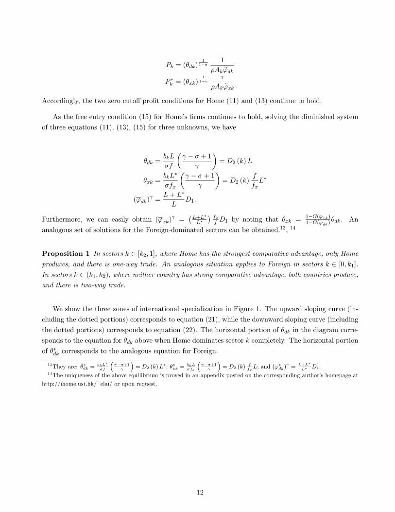
Proposition 1 In sectors k 2 [k2; 1], where Home has the strongest comparative advantage, only Homeproduces, and there is one-way trade. An analogous situation applies to Foreign in sectors k 2 [0; k1].In sectors k 2 (k1; k2), where neither country has strong comparative advantage, both countries produce,and there is two-way trade.

We show the three zones of international specialization in Figure 1. The upward sloping curve (in-

cluding the dotted portions) corresponds to equation (21), while the downward sloping curve (including

the dotted portions) corresponds to equation (22). The horizontal portion of �dk in the diagram corre-

sponds to the equation for �dk above when Home dominates sector k completely. The horizontal portion

of ��dk corresponds to the analogous equation for Foreign.

13They are: ��dk =bkL

�

�f

� ��+1

�= D2 (k)L

�; ��xk =bkL�fx

� ��+1

�= D2 (k)

ffxL; and ('�dk)

= L+L�

L� D1.14The uniqueness of the above equilibrium is proved in an appendix posted on the corresponding author�s homepage at

http://ihome.ust.hk/~elai/ or upon request.

12

0 k

DomesticFirmNumber

dkθ*dkθ

Only Foreign produces

Both countries produce

Only Home produces

11k 2k

Figure 1. Three Zones of International Specialization (assumptions: (i) expenditure shares are

equal across sectors; (ii) L < L�).

4 Opening up to Trade

In this section, we analyze how opening trade between the two countries impacts the economy of

each country, e.g. the productivity cuto¤s, the mass of producing and exporting �rms, as well as

welfare. Before proceeding with the analysis, it is helpful to list the solutions to the relevant variables

corresponding to the three types of sectors in Table 1.

13

Sector type Foreign-dominated Two-way trade Home-dominated

k < k1 k1 < k < k2 k > k2

('dk) ? D1

B�B�1B�(ak) D1

L+L�

L

('xk) ? D1

B�B�1B�(ak)�

�1ak

� �Bfxf

�D1

fxf

�L+L�

L��

('�dk) D1

L+L�

L� D1B�B�1B�(ak)�

?

('�xk) D1

fxfL+L�

L D1B�B�1B�(ak) (ak)

�Bfxf

�?

�dk 0 D2 (k)BL� B�(ak)

B(ak) �1L

�

B�B�1 D2 (k)L

�xk 0�'dk'xk

� �dk D2 (k)

ffxL�

��dk D2 (k)L� D2 (k)

BL��B(ak) �1

B�(ak) L

B�B�1 0

��xk D2 (k)ffxL

�'�dk'�xk

� ��dk 0

Pk [D2 (k)L]1

1�� akB1

�L

L+L�

� 1 1�Ak e'ck [D2 (k)L]

11�� 1

�Ak e'dk [D2 (k)L]1

1�� 1�Ak e'dk

P �k [D2 (k)L�]

11�� 1

�A�k e'�dk [D2 (k)L�]

11�� 1

�A�k e'�dk [D2(k)L�]1

1��

�A�k e'�ck B1

ak

�L�

L+L�

� 1

Table 1: Solution of the System

D1 =

�� � 1

� � + 1

�f

fe; D2 (k) =

� � � + 1

�bk�f

; (ak1) =

B�LL� + 1

�B2 LL� + 1

; (ak2) =

B2L�

L + 1

B�L�L + 1

�4.1 Impacts on productivity cuto¤s

In this subsection, we analyze how trade a¤ects the productivity cuto¤s from two aspects: within sector

and across sectors. First, we look at how trade integration changes the cuto¤s within a certain sector.

In this regard, we �nd that the impacts of trade integration on productivity cuto¤s are the same as

in Melitz (2003) in all sectors. Then we compare the cuto¤s across sectors upon trade integration.

We add a subscript c to all the parameters pertaining to autarky (c=closed economy). It has been

shown in Section 2 that the autarky productivity cuto¤ for survival in Home and Foreign is given by

('ck) = ('�ck)

=�

��1 ��+1

�ffe= D1. If both countries produce, then the equilibrium cuto¤s for

survival are given by (17) and (18). As (ak) 2

�1B , B

�, we have 'dk > 'ck and '

�dk > '

�ck.

Recall that if only one country produces, the equilibrium productivity cuto¤s for survival are

given by:

('dk) =

L+ L�

LD1 > ('ck)

if only Home produces

('�dk) =

L+ L�

L�D1 > ('

�ck)

if only Foreign produces

Hence, the least productive �rms in all sectors will exit the market after trade integration. As a

result, resources will be reallocated to the most productive �rms. Furthermore, 'dk > 'ck implies thate'dk > e'ck, and '�dk > '�ck implies that e'�dk > e'�ck. Therefore, the average productivity in any sector k14

is higher under trade integration than in autarky. Thus we generalize Melitz�s result to a setting where

there exist endogenous intra-industry trade and inter-industry trade in a uni�ed model.

In the closed economy, the cuto¤s for survival are identical across sectors. However, this is not true

any more in the open economy. In the sectors where both countries produce, the equilibrium cuto¤ for

survival is an increasing function of the sectoral comparative advantage. More precisely, as ak increases,

'dk rises but '�dk falls, and, following the free entry conditions (15) and (16), 'xk falls but '

�xk rises.

Thus, we have

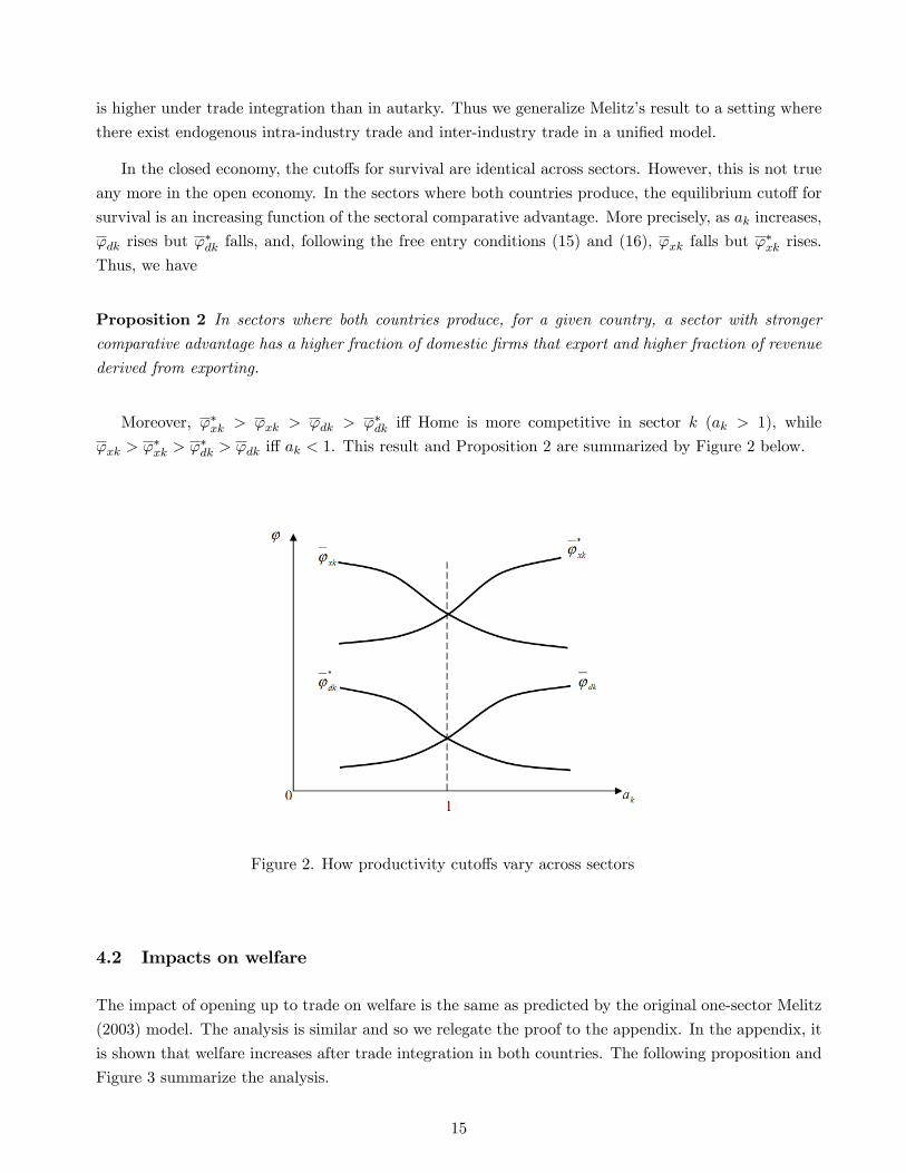
Proposition 2 In sectors where both countries produce, for a given country, a sector with strongercomparative advantage has a higher fraction of domestic �rms that export and higher fraction of revenue

derived from exporting.

Moreover, '�xk > 'xk > 'dk > '�dk i¤ Home is more competitive in sector k (ak > 1), while

'xk > '�xk > '

�dk > 'dk i¤ ak < 1. This result and Proposition 2 are summarized by Figure 2 below.

Figure 2. How productivity cuto¤s vary across sectors

4.2 Impacts on welfare

The impact of opening up to trade on welfare is the same as predicted by the original one-sector Melitz

(2003) model. The analysis is similar and so we relegate the proof to the appendix. In the appendix, it

is shown that welfare increases after trade integration in both countries. The following proposition and

Figure 3 summarize the analysis.

15

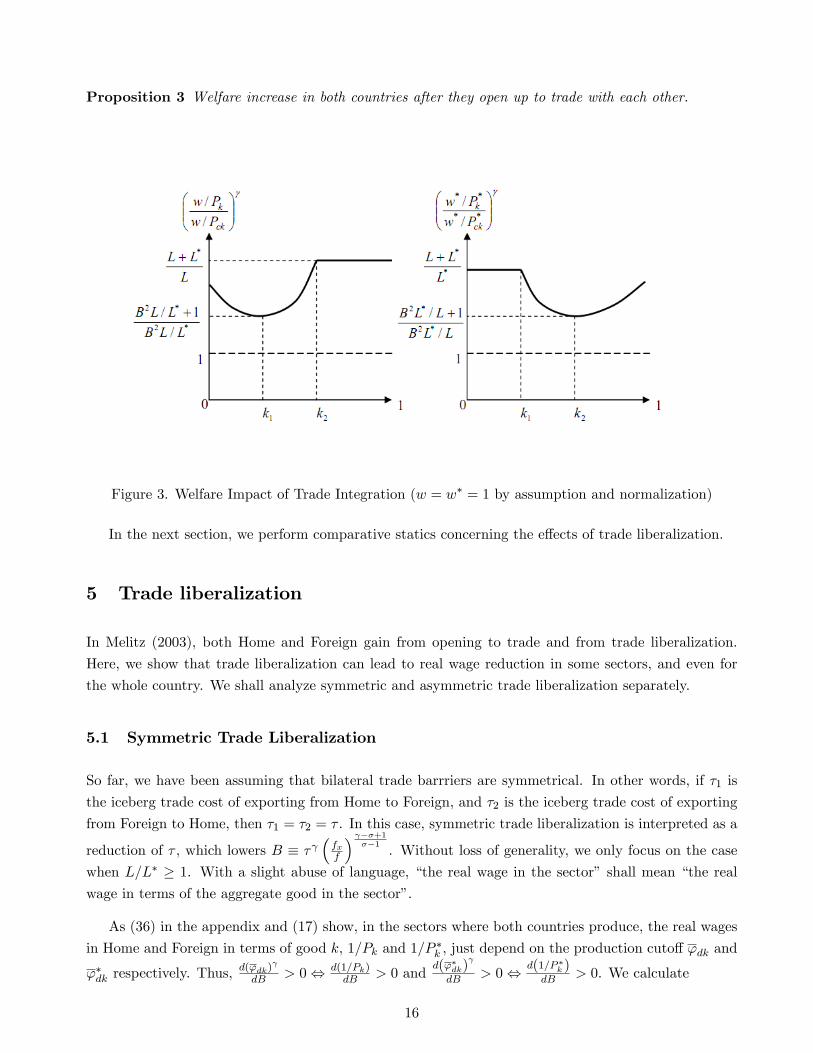
Proposition 3 Welfare increase in both countries after they open up to trade with each other.

Figure 3. Welfare Impact of Trade Integration (w = w� = 1 by assumption and normalization)

In the next section, we perform comparative statics concerning the e¤ects of trade liberalization.

5 Trade liberalization

In Melitz (2003), both Home and Foreign gain from opening to trade and from trade liberalization.

Here, we show that trade liberalization can lead to real wage reduction in some sectors, and even for

the whole country. We shall analyze symmetric and asymmetric trade liberalization separately.

5.1 Symmetric Trade Liberalization

So far, we have been assuming that bilateral trade barrriers are symmetrical. In other words, if �1 is

the iceberg trade cost of exporting from Home to Foreign, and �2 is the iceberg trade cost of exporting

from Foreign to Home, then �1 = �2 = � . In this case, symmetric trade liberalization is interpreted as a

reduction of � , which lowers B � � �fxf

� ��+1��1

. Without loss of generality, we only focus on the case

when L=L� � 1. With a slight abuse of language, �the real wage in the sector� shall mean �the real

wage in terms of the aggregate good in the sector�.

As (36) in the appendix and (17) show, in the sectors where both countries produce, the real wages

in Home and Foreign in terms of good k, 1=Pk and 1=P �k , just depend on the production cuto¤ 'dk and

'�dk respectively. Thus,d('dk)

dB > 0, d(1=Pk)dB > 0 and

d('�dk)

dB > 0, d(1=P �k )dB > 0. We calculate

16

d ('dk)

dB=2B�1 �

�1 +B�2

�(ak)

[B � (ak) ]2(25)

d ('�dk)

dB=2B�1 �

�1 +B�2

�(ak)

� �B � (ak)�

�2 (26)

which shows that 'dk increases with B (and 'xk decreases with B according to (15) ) if and only if

(ak) < 2B

1+B2. Moreover, '�dk increases with B (and '

�xk decreases with B according to (16)) if and only

if (ak) > 1+B2

2B . Recalling that (ak1) =

B( LL�+1)B2 L

L�+1and (ak2)

=B2 L

�L+1

B(L�L+1), and comparing them with the

above thresholds, we can obtain the following conclusions. (i) When L = L�, k1 and k2 exactly coincide

with these thresholds, meaning that in the two-way trade sectors, 'dk (as well as real wage in sector k)

always decreases with B, and 'xk always increases with B. In other word, Melitz�s predictions hold in

this case. (ii) As L=L� increases above one, k1 decreases, and there exist some two-way trade sectors

k 2hk1;

2B1+B2

i, in which 'dk increases with B and 'xk decreases with B. That is, symmetric trade

liberalization leads to a decrease in the productivity cuto¤ for survival but an increase in the exporting

cuto¤. Moreover, the real wage in these sectors also fall. These are all opposite to the predictions of the

original Melitz model. Thus, we call this the �reverse-Melitz outcome�. (iii) As L=L� increases above

one, k2 decreases, and so there does not exist any sector in which '�dk increases with B or '�xk decreases

with B. Thus, the reverse-Melitz outcome does not exist in any sector in the smaller country.

For a more detailed mathematical analysis of the impacts of symmetric trade liberalization, refer to

equations (36) to (38) and to Appendix C.

Figure 4 summarizes the e¤ects graphically. The diagram shows the welfare e¤ects of symmetric

trade liberalization. The k1 and k2 curves show the pattern of international specialization for any given

L=L�. (Recall that L=L� � 1 is assumed.) The zone to the left of the k1 curve corresponds to sectorscompletely dominated by Foreign. The zone to the right of the k2 curve corresponds to the sectors

completely dominated by Home. The downward sloping k1 curve indicates that as the relative size of

Home becomes larger, it can pro�tably produce in more sectors. This shows the home market e¤ect as

explained by Krugman (1980) � the �rms located in the larger country has the advantage of saving the

trade costs of serving the larger market, which more than compensates for its cost disadvantage relative

to the �rms located in the smaller country in the same sector. On the other hand, the downward sloping

k2 curve shows that Foreign, the smaller country, can pro�tably produce in fewer sectors as the relative

size of Home increases. This reminds us of the result in Markusen and Venables (2000), in which they

�nd that the larger country can export a good in which it has comparative disadvantage because of

home market e¤ect. As will be shown later, this explains why the �reverse-Melitz outcome�can only

occur in the larger country under symmetric trade liberalization or symmetric trade cost reduction.

The �gure also shows, for any given value of L=L�, the signs of the real-wage e¤ect of symmetric

trade liberalization on Home and Foreign in di¤erent sectors. The upper sign inside a rectangle indicates

the sign of Home�s change in real wage in terms of good k due to an in�nitesimal decrease in � , and

the lower sign indicates the sign of Foreign�s change in real wage in terms of good k. For example, for

1 < L=L� < B2 (indicated by the arrow on the vertical axis in Figure 4), when there is an in�nitesimal

17

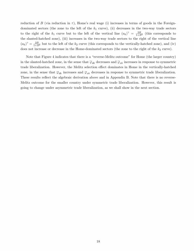
reduction of B (via reduction in �), Home�s real wage (i) increases in terms of goods in the Foreign-

dominated sectors (the zone to the left of the k1 curve), (ii) decreases in the two-way trade sectors

to the right of the k1 curve but to the left of the vertical line (ak) = 2B

1+B2(this corresponds to

the slanted-hatched zone), (iii) increases in the two-way trade sectors to the right of the vertical line

(ak) = 2B

1+B2but to the left of the k2 curve (this corresponds to the vertically-hatched zone), and (iv)

does not increase or decrease in the Home-dominated sectors (the zone to the right of the k2 curve).

Note that Figure 4 indicates that there is a �reverse-Melitz outcome�for Home (the larger country)

in the slanted-hatched zone, in the sense that 'dk decreases and 'xk increases in response to symmetric

trade liberalization. However, the Melitz selection e¤ect dominates in Home in the vertically-hatched

zone, in the sense that 'dk increases and 'xk decreases in response to symmetric trade liberalization.

These results re�ect the algebraic derivation above and in Appendix B. Note that there is no reverse-

Melitz outcome for the smaller country under symmetric trade liberalization. However, this result is

going to change under asymmetric trade liberalization, as we shall show in the next section.

18

Figure 4. Welfare E¤ects of Symmetric Trade Liberalization (in�nitesimal reduction of B through a

reduction of �). In each region, the upper sign inside the rectangle indicates the welfare

change of Home and the lower sign indicates the welfare change of Foreign. The short

horizontal arrows indicate the movement of lines as B falls.

As B decreases, the curves for k1 and k2, as well as the vertical lines corresponding to (ak) = 2B

B2+1

and (ak) = B2+1

2B , will all shift, with the directions of shifts shown by the small horizontal arrows in

Figure 4. For any given L=L�, as � (and therefore B) decreases from a large number, k1 increases, k2�rst decreases then increases, (ak)

= 2BB2+1

increases while (ak) = B2+1

2B decreases.

Depending on the range of [a0, a1] and the value of L=L�, it is possible that the k1 or k2 curve (or

both) may situate outside the range k 2 [0; 1] for some or all values of L=L�. For example, if ak1 < a0 fora given value of L=L�, then no Foreign-dominated sector exist for that value of L=L�. This is because

as L=L� gets su¢ ciently large, the home-market e¤ect in Home gets so strong that Home can compete

19

even in the sector in which it has the weakest comparative advantage, namely sector k = 0.

The above discussion and Figure 4 can be summarized by the following lemma and proposition:

Lemma 2 When the two country are of the same size, symmetric trade liberalization improves the realwages in all two-way trade sectors in both countries.

Proposition 4 Consider the sectors in which both countries produce. Suppose Home is larger thanForeign. In the sectors where Home has the strongest comparative disadvantage but still produces, there

is a reverse-Melitz outcome in the sense that 'dk decreases while 'xk increases in the face of symmetric

trade liberalization, leading to reduction in Home�s real wage in these sectors.

Proposition 4 deserves more discussion, as it highlights one of the most important results of this

paper. If Home is the larger country, the sectors in which its real wage deceases upon symmetric trade

liberalization are de�ned bynk j (ak1)

< (ak) < (ak2)

and (ak) < 2B

1+B2

o. The �rst condition in-

dicates that the sector is a two-way trade sector. The second condition indicates that the sector is

among those in which the larger country has the weakest comparative advantage. The two conditions

combined says that, in the sectors where the larger country has the weakest comparative advantage yet

still produces, Home�s real wage decreases with symmetric trade liberalization. In other words, there

is a reverse-Melitz outcome in these sectors, i.e. 'dk decreases while 'xk increases in the face ofsymmetric trade liberalization, leading to a decrease in the average productivity of �rms serving the

Home market, thus lowering real wage in that sector. We can explain the existence of the reverse-

Melitz outcome by decomposing the total e¤ect of symmetric trade liberalization into two e¤ects: the

Melitz selection e¤ect and the inter-sectoral resource allocation (IRA) e¤ect. We shall analyze from the

perspective of Home and Home�s �rms.

� Note that the number of potential entrants in sector k in Home is given by

nk =�dk

1�G ('dk)= �dk ('dk)

= D1D2 (k)

�BL

B � (ak) � L�

B (ak) � 1

�(27)

and recall

�dk = D2 (k)

24BL� B�(ak) B(ak)

�1L�

B �B�1

35 (21)

('dk) = D1

�B �B�1B � (ak)

�(17)

d ('dk)

dB=2B�1 �

�1 +B�2

�(ak)

[B � (ak) ]2(25)

1

Pk=

�B �B�1B � (ak)

� 1 1

Pck(36) from the appendix

20

� When L = L�, and ak = 1, 8k, our model collapses to the Melitz model with a homogenous-goodsector. (27) implies that nk = D1D2 (k)L. With symmetric trade liberalization, the numbers

of potential entrants nk and n�k will remain unchanged. Note that (17) implies that ('dk) =

D1�B+1B

�. Therefore, d('dk)

dB < 0. That is, real wages in all sectors rise with symmetric trade

liberalization. As a result, the export revenue of a typical exporting �rm will increase as trade

cost falls. This creates pressure for both 'xk and '�xk to decrease. Meanwhile, this willforce the least productive �rms in each country to exit, as there are more �rms exporting to the

domestic market. This creates pressure for both 'dk and '�dk to increase. The increase inaverage productivity in all sectors lead to increase in real wage in all sectors. This is the Melitzselection e¤ect, which is the only e¤ect here. Thus, we have the Melitz outcome.

� Next, we allow ak to deviate from 1 for some k, but keep L = L�. This creates compara-

tive advantage for Home in some sectors and comparative disadvantage for Home in other sec-

tors. Note that (25) holds only if sector k satis�es the constraint for two-way trade, given by

(ak1) < (ak)

< (ak2) . Observe that (i) (23) implies that (ak1)

< (ak) is equivalent to

2B�1 ��1 +B�2

�(ak)

< 0; therefore, (25) implies that d('dk)

dB < 0 for all two-way trade sec-

tors. In other words, symmetric trade liberalization always increases the real wage in a two-way

trade sector. That is, the Melitz selection e¤ect dominates in all two-way trade sectors as long as

L = L�. (ii) (25) implies that���d('dk) dB

��� increases with ak. That is, the dominance of the Melitze¤ect in a sector decreases as the comparative advantage of Home diminishes. (iii) (23) implies

that at k = k1, 2B�1 ��1 +B�2

�(ak)

= 0, which in turn implies that d('dk)

dB = 0. That is,

the Melitz selection e¤ect is completely o¤set in sector k1, the sector in which Home has the least

comparative advantage yet still produces. What happens to make���d('dk) dB

��� increase with ak? Thee¤ect comes from re-allocation of resources (labor) between sectors as B decreases, which we call

inter-sectoral resource allocation (IRA) e¤ect. Symmetric trade liberalization leads to re-sources in Home (as well in Foreign) being re-allocated away from the di¤erentiated-good sectors

in which it has comparative disadvantage to ones in which it has comparative advantage (and

possibly the homogeneous good sector). Therefore, nk decreases and n�k increases in the sectors

in which Home has comparative disadvantage. As n�k increases, Foreign�s market becomes more

competitive (as there are more �rms in Foreign) and so rxk (') decreases for all '. This createspressure for an increase in 'xk (i.e. only the more productive Home �rms can pro�tably

export now). As nk decreases, �dk also decreases. This leads to the expansion of the sizes of the

surviving Home �rms. Thus, rdk (') increases for all '. This creates pressure for a decreasein 'dk as some less productive �rms which were expected to be unpro�table before can be ex-pected to be pro�table now. The IRA e¤ect causes the variables nk, n�k, rxk ('), 'xk, �dk, rdk ('),

'dk to move in opposite directions in the sectors in which Home has comparative advantage. In

other words, the IRA e¤ect reinforces the Melitz selection e¤ect in the sectors in which Home has

comparative advantage but counteracts the Melitz e¤ect in the sectors in which it has comparative

disadvantage.15 Observations (ii) and (iii) above indicate that the IRA e¤ect is stronger when

Home has weaker comparative advantage in the sector. However, as long as L = L�, the IRA15The de�nition of a comparative advantage sector is bound to be subjective. Here, we de�ne a sector to be a comparative

advantage (disadvantage) sector if nk increases (decreases) as � decreases.

21

e¤ect never dominates the Melitz selection e¤ect, as each country cannot pro�tably produce goods

in which it does not have su¢ ciently strong comparative advantage. Without any home market

e¤ect, the range of goods produced by Home is limited by its comparative advantage. Therefore,

there is still no reverse-Melitz outcome in any sector.

� Next, we allow L= L� to increase above one, in addition to ak 6= 1 for some k. Now, because

of increasing returns to scale and the home market e¤ect as explained in Krugman (1980), it is

possible for the IRA e¤ect to dominate the Melitz selection e¤ect in Home, as Home is now able to

pro�tably produce goods that it was not able to when L = L�. In other words, because of its large

size, Home is now able to pro�tably produce goods in which it has comparative disadvantage. In

these sectors, d('dk)

dB < 0 � the IRA e¤ect dominates the Melitz selection e¤ect, and we have the

reverse-Melitz outcome. However, Foreign, the smaller country, can never have reverse-Melitzoutcome in any sector, because it is not able to pro�tably produce any good that it was not able

to when L = L�.

As the IRA e¤ects in the comparative advantage sectors are positive, there are gains in real wage in

terms of these sectors�goods upon symmetric trade liberalization. Can these gains o¤set the losses in the

comparative disadvantage sectors mentioned above? The answer is, it depends on Home�s relative size.

If Home�s relative size is large, and the Foreign-dominated sector is small, then the gains cannot o¤set

the losses. For example, when B = 2, L=L� = 5, = 2 (and therefore ak1 = 0:756 and ak2 = 0:866);

and suppose a0 = 0:8 (and therefore k1 < 0, which means that there does not exist any sector in

which Foreign completely dominates). Then, Home will unambiguously lose from symmetric trade

liberalization, as it loses in the sectors where k 2 [0; k2], and does not gain or lose in the sectors wherek 2 [k2; 1] and in the homogeneous good sector.

Based on the above analysis, we end this section with the following two propositions:

Proposition 5 Consider the sectors in which both countries produce. Suppose Home is larger thanForeign. In the face of symmetric trade liberalization, the fraction of exporters increases in Home�s

comparative advantage sectors but decreases in the sectors in which Home has the strongest comparative

disadvantage.

Proposition 6 Consider the sectors in which both countries produce. Suppose Home is larger thanForeign. In the face of symmetric trade liberalization, the fraction of revenue derived from exporting

increases in Home�s comparative advantage sectors but decreases in the sectors in which Home has the

strongest comparative disadvantage.

22

5.2 Asymmetric Trade Liberalization

We have shown that reverse-Melitz outcome occurs only in the larger country under symmetic trade

liberalization. However, we shall show below that it occurs even in the smaller country under asymmetric

trade liberalization, if the percentage reduction of importing cost of the smaller country is su¢ ciently

greater than that of the larger country. In the extreme case, unilateral trade liberalization of Home

lowers its real wage in all sectors regardless of its relative size. This result is important as we shall use

it to test the reverse-Melitz outcome in China, which underwent asymmetric trade liberalization upon

its accession to the WTO.

Let �1 denote the trade cost of exporting from Home to Foreign, and �2 denote the trade cost of

exporting from Foreign to Home. In general �1 6= �2 and therefore B1 6= B2. The detailed analysis isrelegated to the Appendix. In the appendix, we prove that (i) Home�s real wage falls in all sectorsas Home unilaterally reduces its tari¤s against Foreign�s exports (we call this unilateralliberalization (UL) e¤ect); and (ii) Home�s real wage rises in all sectors as Foreign unilaterallyreduces its tari¤s against Home�s exports. The UL e¤ect works similarly as the IRA e¤ect in Home�s

comparative disadvantage sectors: nk and �dk both fall, while n�k rises. As n�k increases, it forces up

'xk as Foreign�s market becomes more competitive. As �dk decreases, the revenues of all domestic �rms

increase, forcing down 'dk.

The following equations extracted from the appendix will be useful in the ensuing analysis.

(ak1) =

B1�LL� + 1

�B1B2

LL� + 1

(39)

(ak2) =

B1B2L�

L + 1

B2�L�L + 1

� (40)

d ('dk)

dB2= D1

B�22B1 � (ak)

(41)

d ('dk)

dB1= D1

B�12 � (ak)

[B1 � (ak) ]2(42)

Suppose �1and �2 both decrease so that B1 and B2 both fall.

Assumptions: (a) De�ne � � dB1=dB2 where � > 0; and

(b) jdB1=B1j < jdB2=B2j (which is equivalent to jd�1=�1j < jd�2=�2j, i.e. the percentage reductionin iceberg importing cost is lower in Foreign than in Home).

Note that (a) and (b) imply that B1 > �B2. If reduction in B1 and B2 results in a fall in 'dk, then

23

we have a reverse-Melitze outcome. Therefore, reverse-Melitz outcome exists in a sector i¤

d ('dk)

dB2+ �

d ('dk)

dB1> 0

() B1 + �B2 ��1 + �B22

�(ak)

> 0

() (ak) <

B1 + �B21 + �B22

Thus, we have

Lemma 3 Reverse-Melitz outcome exists in a sector i¤ (ak) < B1+�B2

1+�B22.

Now, consider the case L = L�. Equations (41) and (42) imply that there is reverse-Melitz outcome

when k = k1 (the two-way trade sector in which Home has the weakest compararive advantage) i¤

d ('dk)

dB2+ �

d ('dk)

dB1> 0 at k = k1

() B1 + �B2 ��1 + �B22

�(ak1)

> 0 (28)

() (B1 � �B2) (B1B2 � 1) > 0,

which is true according to our assumption B1 > �B2 and the fact that B1, B2 > 1.

From Lemma 3 and the above result, we can conclude that there is reverse-Melitz outcome for the

sectors satisfying2B1

B1B2 + 1= (ak1)

< (ak) <

B1 + �B21 + �B22

.

Therefore we have

Conclusion 1: There is reverse-Melitz outcome in Home even if L = L�, as long as jd�1=�1j <jd�2=�2j.

The intuition for Conclusion 1 is as follows. We assume L = L� and allow ak to deviate from 1 for

some k. This creates comparative advantage for Home in some sectors and comparative disadvantage

for Home in other sectors. Note that (41) and (42) hold only if sector k satis�es the constraint for

two-way trade, given by (ak1) < (ak)

< (ak2) . Observe that (i) (39) implies that (ak1)

< (ak) is

equivalent to 2B1 � (1 +B1B2) (ak) < 0; therefore, (41) and (42) imply that d('dk)

dB2+ �d('dk)

dB1> 0

at k = k1 i¤ (B1 � �B2) (B1B2 � 1) > 0, which is true as long as jd�1=�1j < jd�2=�2j. In other

words, asymmetric trade liberalization (with jd�1=�1j < jd�2=�2j) lowers the real wage for the two-way trade sectors in which Home has the weakest comparative advantage, i.e. sectors k satisfying2B1

B1B2+1= (ak1)

< (ak) < B1+�B2

1+�B22. That is, the reverse-Melitz outcome exists even when L = L�,

contrary to the case with symmetric trade liberalization. (ii) (41) and (42) imply that d('dk)

dB2+�d('dk)

dB1

24

is negative when ak gets su¢ ciently large.16 That is, there will not be reverse-Melitz outcome in the

sectors in which Home has su¢ ciently strong comparative advantage.

Suppose we allow L 6= L�. For reverse-Melitz outcome to exist, we invoke (39) and (28), by solving forLL� from (ak1)

= B1+�B21+�B22

, and �nd that the reverse-Melitz outcome can occur in the most comparative

disadvantage two-way trade sectors in Home (i.e. k1) as long as

L

L�>�B2B1

=jd�1=�1jjd�2=�2j

The right hand side is less than one. Therefore, we have

Conclusion 2: It is possible for reverse-Melitz outcome to occur in Home under asymmetric tradeliberalization even if Home is smaller than Foreign. More speci�cally, as long as jd�1=�1j < jd�2=�2j,reverse-Melitz outcome exists in sector k1 i¤ L=L� > jd�1=�1j = jd�2=�2j.

We summarize the above conclusions in Propositions 7, 8 and 9 below, which are parallel to Propo-

sitions 4, 5 and 6 respectively.

Proposition 7 Consider the sectors in which both countries produce. If the percentage decrease inHome�s iceberg import cost is more than that of Foreign�s, then 'dk decreases while 'xk increases in the

sectors in which Home has the strongest comparative disadvantage, leading to reduction in Home�s real

wage in these sectors, as long as Home is not too small compared with Foreign.

Proposition 8 Consider the sectors in which both countries produce. If the percentage decrease inHome�s iceberg import cost is more than that of Foreign�s, then the fraction of exporters increases in

Home�s comparative advantage sectors but decreases in the sectors in which Home has the strongest

comparative disadvantage, as long as Home is not too small compared with Foreign.

Proposition 9 Consider the sectors in which both countries produce. If the percentage decrease inHome�s iceberg import cost is more than that of Foreign�s, then the fraction of revenue derived from

exporting increases in Home�s comparative advantage sectors but decreases in the sectors in which Home

has the strongest comparative disadvantage, as long as Home is not too small compared with Foreign.

Discussion. Symmetric trade liberalization is a special case of asymmetric liberalization (with

jd�1=�1j = jd�2=�2j). (In fact, the same results as in the symmetric case analyzed in the last subsectionobtain even when �1 6= �2.) We can think of asymmetric liberalization (with Home liberalizing more

than Foreign, i.e. jd�1=�1j < jd�2=�2j) as the combination of symmetric liberalization and unilateral16As (28) shows, the reverse-Melitz outcome requires that B1 + �B2 �

�1 + �B2

2

�(ak1)

be positive. However, the

expression gets smaller as ak1 increases.

25

liberalization by Home. Symmetric liberalization has been thoroughly analyzed in the last subsection.

It leads to the reverse-Melitz outcome in Home�s most comparative disadvantage two-way trade sectors

if Home is larger than Foreign. Unilateral liberalization by Home leads to reduction of real wage in all

sectors in Home, contributing to an additional reason for the existence of the reverse-Melitz outcome.

We call this unilateral liberalization e¤ect (UL e¤ect). The UL e¤ect explains why reverse-Melitz

outcome occurs under asymmetric liberalization even when Home is smaller than Foreign. Note that

reduction of real wage occurs even in a one-sector model (with say ak = 1). When we combine the Melitz

selection e¤ect, IRA e¤ect and UL e¤ect, the impact of asymmetric trade liberalization on real wage

again turns from negative to positive as the comparative advantage of the sector increases, like in the

case of symmetric liberalization. Thus, there is reverse-Melitz outcome only for the most comparative

disadvantage sectors, as in the case with symmetric trade liberalization. We expect a large country

undergoing asymmetric trade liberalization to be likely to exhibit reverse-Melitz outcome. The episode

of trade liberalization by China following its accession to WTO in 2001 is a good candidate to test our

theory, as China was large, and the trade liberalization episode then was quite asymmetric. Therefore,

in Section 7 we shall test propositions 8 and 9 using Chinese data. Before that, we �rst discuss in the

next section a possible extension of our model to capture another interesting phenomenon in China�s

trade recently documented.

6 Can �rms that sell domestically be more productive than �rmsthat don�t?

Recently, there has been some discussion of the existence of another �reverse-Melitz outcome�. Lu

(2010) shows that, theoretically, in a multi-sector Melitz model, the average productivity of exporters

can be lower than that of the �rms that serve the domestic market in the comparative advantage sectors.

She then supports her theory by the empirical �nding that, in the comparative advantage sectors, the

exporters in China have a relative lower average productivity compared with the �rms that serve the

domestic market. This e¤ect, though also contrasts sharply with Melitz�s one-sector result, is completely

di¤erent from the one explained in section 5. Nonetheless, it is still worth asking whether our model

can be made consistent with this e¤ect. The answer is yes.

So far, we simpli�ed our analysis by assuming that fxf > maxfLL� ;

L�

L g so as to exclude the possibilitythat some �rms only export but do not serve the domestic market. Our model can in fact be modi�ed to

accommodate this possibility by relaxing this assumption. First of all, we adopt the assumption that a

�rm needs to incur a market entry cost if it enters a market, be it domestic or foreign. Now, let f and fxstand for the �xed market-entry cost plus the overhead cost for serving the domestic market and foreign

market respectively.17 In this case, we can relax the assumption fxf > maxf

LL� ;

L�

L g (only ���1fx > f

is needed), and all of our propositions still hold. In the appendix, we show that when fx is su¢ ciently

smaller than f , then we can have a situation where the cuto¤ productivity for exporting is lower than

the cuto¤ productivity for selling domestically in the comparative advantage sectors. Thus, the average

17This is di¤erent from the original assumption in Melitz (2003) as well as in this paper so far.

26

productivity of the �rms that export is lower than the average productivity of �rms that both export

and sell domestically in the comparative advantage sector. The main point is that it is possible that for

some sector k, we have 'dk > 'xk. Once we have this outcome, we can have the situation where some

�rms in the sectors where a country has the strongest comparative advantage may only export; thus

in these sectors the �rms that only export are less productive than those that also serve the domestic

market. This is also consistent with Lu�s (2012) �nding that in labor-intensive sectors, �rms that serve

domestic market have higher productivity than exporters, as China has comparative advantage in the

labor-intensive industries.

Detailed calculation is given in the appendix. We state our result in

Proposition 10 If the �xed entry cost for exporting is not too high, then in the sectors where a countryhas the strongest comparative advantage, the �rms that do not serve the domestic market can have a

lower average productivity than those that do.

One major characteristic of the Chinese exporting sector is that a large fraction of exporting �rms

engage in processing trade, and they mostly concentrate in the labor-intensive sectors, which are the

comparative advantage sectors of China. Export processing in China is subject to very di¤erent policy

treatment compared to non-processing trade. First, processing activities enjoy favorable taxation. The

amount of imported inputs actually used in the making of the �nished products for export is exempt

from tari¤s and import-related taxes. All processed �nished products for export are also exempt from

export tari¤s and value-added tax. Second, the �nished products using the tax-exempted materials

have to be re-exported, and enterprises are not allowed to sell the tax-exempted materials and parts

or �nished products in China. The assumption that the �xed cost for exporting �rms is relatively low

compared with the �xed cost for �rms selling in the domestic market �ts the observation that the cost

of entry into processing trade in China is relatively low because of government policy.

According to Dai, Maitra and Yu (2011), �In China roughly a �fth of exporters, accounting for

about one-third of total export value, are engaged in processing trade only. These �rms are 4% to 30%

less productive than non-exporters.�They go on to say, �Our data shows that processing trade �rms

pay lower average wages implying that they are more unskilled labor intensive, are relatively less capital

intensive, and have low pro�tability compared to non-processing ones. Given that processing �rms pay

lower �xed cost (due to government intervention) it makes sense that only the low productivity �rms

would select into processing trade.�These �ndings are all consistent with this modi�ed version of our

model.

Thus, our theoretical model can indeed be extended to include both types of non-standard e¤ects.

Next, we move on to some emprical evidence. The empirical evidence for Lu�s (2010) e¤ect has already

been o¤ered by her. In the next section, we present the empirical tests of our two major propositions.

27

7 Empirical Tests of Propositions 8 and 9

Propositions 8 and 9 in section 5 predict the existence of a reverse-Melitz outcome: For a su¢ ciently

large country, like China, in the sectors where it has the strongest comparative disadvantage but still

produces, the fraction of �rms that export and the share of revenue derived from exporting will both

decrease upon asymmetric trade liberalization such that the percentage reduction of China�s trade cost

is lower than that of its trading partners. Can we �nd any evidence to support the existence of the

reverse-Melitz outcome? This section shows that we indeed �nd evidence of such an e¤ect.

China acceded to the WTO in December 2001. Since then there was a series of tari¤ reductions for

a number of years. It is well-documented that the conditions of WTO accession require China to reduce

its import barriers with very little corresponding changes in its trade partners�import barriers against

China. Therefore, this kind of asymmetric trade liberalization (that the percentage reduction in China�s

iceberg import cost is higher than those of its trading partners) �ts the description in Propositions 8

and 9 very well. We should therefore expect the comparative disadvantage sectors of China to exhibit

reverse-Melitz outcome while the comparative advantage sectors to exhibit Melitz outcome.

We test the theory at the 4-digit CIC level, using Chinese industrial �rm data from National Bureau

of Statistics of China (NBSC), Chinese Customs data from China�s General Administration of Customs

and tari¤ data from the World Trade Organization (WTO). To get a panel of variables, we need to �rst

tackle the problem caused by a major revision to the Chinese Industry Classi�cation (CIC) in the year

2002. In order to have a consistent de�nition of sectors, we follow Brandt, Van Biesebroeck & Zhang

(2012) by adjusting the 4-digit CIC so as to make the same industry classi�cation code representing

the same industry both before and after year 2002.18 After adjusting the CIC code for each sector, we

aggregate the variables at the 4-digit sector level and obtain a panel of aggregate variables (e.g. mass

of �rms, mass of �rms that export, total revenue, total exporting revenue, etc.) from the years 2001 to

2006, and then calculate the variables we need.19

In order to test the e¤ect of trade liberalization, we also need to establish a proper measure of trade

cost � . As transportation cost is hard to measure and should not vary much in a few years�time, we

take the tari¤ rate, which decreased a lot after China joined the WTO, as the measure of trade cost.

It is also noteworthy that the tari¤ rates for di¤erent sectors are di¤erent, which is not consistent with

the assumption of our model. Fortunately, it turns out that the results and equations of the model will

not be qualitatively a¤ected by the heterogeneity of trade costs across sectors. Therefore, we take into

consideration the heterogeneity of tari¤ rates across sectors in calculating which sectors are predicted

to exhibit the reverse-Melitz outcome according to the theory. More explanation is provided below.

Following Amiti and Konings (2007), Goldberg, Khandelwal, Pavcnik and Topalova (2010) and Ge,

Lai and Zhu (2011), we construct the industry tari¤ rate through aggregating tari¤s to the 4-digit CIC

18The detail of the matching can be found at http://www.econ.kuleuven.be/public/N07057/CHINA/appendix/19The choice of the years is based on the fact that China acceded to World Trade Organization in December 2001, which

further integrated the country with the world. Under the WTO commitments, China cut average tari¤ from 15.4% in 2001

to 5.31% in 2006.

28

level. Like the CIC, there was a major reclassi�cation in the international HS 6-digit codes in 2002.

Hence we also construct a mapping of the 6-digit HS coding system from the pre-2002 to the post-2002

periods. With these matchings in place, we assign each 8-digit HS product to the 6-digit HS code to

which it belongs, and then connect this 6-digits HS code with the standardized 4-digit CIC code, for

each year.20 Finally, we calculate the industry tari¤ as the import-value-weighted average of all 8-digit

HS products which fall into the same 4-digit CIC code for each year. To be precise, the industry tari¤ is

calculated from �it =�PGi

g=1vgt�gt

�=�PGi

g=1vgt

�, where �gt is the 8-digit HS level tari¤ of an imported

good g at year t, vgt is the import value of good g in that year, and Gi is the number of 8-digit HS sectors

included in 4-digit CIC sector i. Later, we use these tari¤ data to test our theory. These industry tari¤s

are the tari¤s faced by foreign �rms entering the Chinese market. As a robustness check, we use the

import value in 2003 (which is the middle year of our sample), vg2003 , as the weight for tari¤ calculation

for all years and rerun all the tests. The purpose of doing so is to control for the variation of trade value

within industry across years during the trade liberalization period so that we can get a clearer picture

of the pure e¤ect of tari¤ reduction.

In addition to allowing tari¤ rate to be di¤erent across sectors, we also allow the elasticity of

substitution �, and the productivity dispersion level to be di¤erent across sectors. It can be shown

that the results listed in Table 1A are qualitatively the same as before. The only change needed in Table

1A in the Appendix is to change B1 to Bk1 � (��k ) �k�fxf

� �k��k�1�1 and B2 to Bk2 � (�k)

k�fxf

� k�k�1

�1. It

follows that Propositions 8 and 9 continue to hold. We further assume that � (� dB1=dB2 where B1 isimport barrier of Foreign and B2 is import barrier of Home) is di¤erent across sectors. Thus, we de�ne

Bk1 as the import barrier of Foreign in sector k and Bk1 as the import barrier of Home in sector k, and

�k � dBk1=dBk2 . Now, di¤erent sectors have di¤erent threshold for ak: (ak) k <

Bk1+�kBk2

1+�k(Bk2 )2 according to

Lemma 3. In other words, the theory predicts that the reverse-Melitz outcome will occur in the two-way

trade sectors in which the relative productivity index (ak) is less than Bk1+�kB

k2

1+�k(Bk2 )2 . Furthermore, from

the version of Table 1A modi�ed for di¤erences in and � across sectors, we can easily verify that the

fraction of �rms that export in each sector satis�es:

�xk�dk

=

�'dk'xk

� k=

1

Bk2� B

k2 (ak)

k � 1Bk1 � (ak) k

� ffx

() �xk�dk

�Bk2

�2= Bk2

�Bk2 (ak)

k � 1Bk1 � (ak) k

�f

fx

Thus, the condition for reverse-Melitz outcome to occur in sector k can be re-written as below:

(ak) k <

Bk1 + �kBk2

1 + �k�Bk2�2 () Bk2

�Bk2 (ak)

k � 1Bk1 � (ak) k

�<1

�k

() Bk2

�Bk2 (ak)

k � 1Bk1 � (ak) k

�f

fx<

f

�kfx() �xk

�dk

�Bk2

�2<

f

�kfx

where the last equivalence is obtained by invoking the previous equation.

20The NBSC provide a concordance table between the 6-digit HS code and the 4-digit Chinese industry code. Source of

this table can be found at: http://www.5000.gov.cn/release/FrontManage/next_page.aspx?currentPosition=2&cateid=2.

29

Therefore, �xk�dk�Bk2�2< f

�kfxi¤ there is reverse-Melitz outcome in sector k. Unfortunately, we do

not have data of �k, as it requires knowing the export barriers of China�s exports to all its trading

partners, which is a daunting task. Therefore, we take a short cut: we assume that �k is randomly

distributed across sectors with mean �. As there is no reason to suspect that �k is correlated with k, this

assumption is justi�able. This assumption is equivalent to saying that �k is i.i.d. with mean �, which

in turn implies that there is more likely to be reverse-Melitz outcome in a sector k when �xk�dk

�Bk2�2is

smaller. We calculate the variable �xk�dk

�Bk2�2, which we call RATIO, for each of the twenty-nine 2-digit

CIC sectors, and rank them. Note that a lower RATIO is assigned a lower rank. A higher RATIO implies

that China has stronger comparative advantage in that sector.21 Table 2 shows the ranking of these

2-digit CIC sectors and the corresponding sectoral information that determine the RATIO. We choose

the eight sectors with the lowest RATIOs to test for the reverse-Melitz outcome and the eight sectors

with the highest RATIOs to test for the Melitz outcome. We run (i) the fraction of exporting �rms and

(ii) the share of exporting revenue, on the tari¤ rate for each 4-digit sector, while controlling for the

year and industry (2-digit CIC level) �xed e¤ects and other relevant variables (including employment,

capital-labor ratio, average wage in each 4-digit sector). Amongst these variables, employment stands

for the size of the sector, and is used to control for the economies of scales; K/L = capital-labor ratio

is used to control for production technique; average wage is used to control for the variable costs and

worker skill. The right hand side variables we choose are similar to those of Bernard, Jensen and Schott

(2006, Table 4). The results are shown in Tables 3A and 3B. (CA stands for comparative advantage.)

<Table 2 about here>

From Tables 3A and 3B, we see that all the coe¢ cients for the variable �Tari¤� are signi�cant

in both regressions. Most importantly, the signs are distinctly positive for the eight comparative-

disadvantage sectors and distinctly negative for the eight comparative-advantage sectors. In other

words, both the fraction of exporting �rms and the share of exporting revenue decrease (increase)

with trade liberalization for the sectors in which China has comparative disadvantage (comparative

advantage). Therefore, we conclude that, consistent with our theory, there exists reverse-Melitz outcome

in the sectors where China has the comparative disadvantage but still produces; while the Melitz

outcome continues to prevail in the sectors in which China has comparative advantage. The coe¢ cients

of the other right hand side variables make sense too. For example, higher K/L signi�es stronger

comparative disadvantage, which lowers exporting ratio and share of export revenue according to our

21Based on a nested constant-elasticity-substitution utility function, Broda and Weinstein (2006) estimate product-

speci�c elasticities of substitution at the HS 10-digit level. The data is available from Weinstein�s website. We aggregate

these numbers up to the HS6 level by taking means, and then use the concordance table from NBSC to calculate the

elasticity of substitution of each sector as the average of all the 6-digit HS products which fall into the standardized 2-digit

CIC code. For the Pareto location parameter k, we estimate them using the estimates of �k and the theoretical prediction

that �rm sales follow a Pareto distribution with shape parameter k�k�1

within industry k. We follow Eaton, Kortum and

Kramarz (2011) in restricting attention to exporters only and back out the shape parameter of the �rm sales distribution

from a regression of the logarithm of the �rm sales rank on the logarithm of �rm sales. As in Axtell (2001), we �nd that k

�k�1is close to 1 for each sector. Hence, we have Bk � � kk and we use � kk to approximate Bk, where �k is the average

tari¤ rate in each 2-digit CIC industry and k captures the productivity dispersion level in each 2-digit CIC industry.

30

theory. Higher wage signi�es higher labor quality, which tends to induce higher propensity to export.

Higher employment signi�es higher economic scale, which also tends to induce higher propensity to

export.

Fraction of exporting �rms, year 2000-2006

Regressor eight sectors with weakest CA eight sectors with strongest CA

Tari¤ 0.593��� 0.754��� 0.542��� -0.420��� -0.180��� -0.144���

(0.125) (0.158) (0.151) (0.065) (0.051) (0.050)

log(employment) -0.002 0.014���

(0.005) (0.004)

log(K/L) -0.128��� -0.095���

(0.015) (0.015)

log(wage) 0.198��� 0.087���

(0.033) (0.029)

Industry �xed e¤ect NA Yes Yes NA Yes Yes

Year �xed e¤ect NA Yes Yes NA Yes Yes

Observations 474 474 474 564 564 564

Note: ���Signi�cant at the 1% level; ��Signi�cant at the 5% level; �Signi�cant at the 10% level.

Table 3A

Share of exporting revenue in total revenue, year 2000-2006

Regressor eight sectors with weakest CA eight sectors with strongest CA

Tari¤ 0.558��� 0.646��� 0.422��� -0.442��� -0.225��� -0.208���

(0.133) (0.150) (0.139) (0.068) (0.052) (0.049)

log(employment) 0.002 0.008��

(0.005) (0.004)

log(K/L) -0.138��� -0.123���

(0.014) (0.015)

log(wage) 0.139��� -0.015

(0.031) (0.028)

Industry �xed e¤ect NA Yes Yes NA Yes Yes

Year �xed e¤ect NA Yes Yes NA Yes Yes

Observations 474 474 474 564 564 564

Note: ���Signi�cant at the 1% level; ��Signi�cant at the 5% level; �Signi�cant at the 10% level.

Table 3B

The choice of the eight sectors with the lowest RATIOs to stand for comparative disadvantage sectors

and the eight sectors with the highest RATIOs to stand for comparative advantage sectors may sound a

bit arbitrary. Therefore, we check the robustness of the results by varying the set of sectors we choose.

We run six regressions for each set of sectors we choose: we run (i) the fraction of exporting �rms and (ii)

the share of exporting revenue, on the tari¤ rate for each set of sectors, while controlling for the year and

industry (2-digit CIC level) �xed e¤ects and other relevant variables (including employment, capital-

31

labor ratio, average wage in each 4-digit sector). Each regression is the same as the corresponding one

shown in Tables 3A and 3B, though the set of sectors used is di¤erent. The result is shown in Figure 5.

Figure 5.

The horizontal axis in Figure 5 indicates what sectors are included when running the regressions.

Note that there is a set of bars on the left and another set of bars on the right. On the left, a number x

on the horizontal axis indicates that sectors from the sector with ranking number 1 to the sector with

ranking number x are included in the regressions. Therefore, as x increases, the number of comparative

disadvantage sectors included in the regressions increase. On the right, a number x indicates that

sectors from the sector with ranking number x to the sector with ranking number 29 are included in

the regression. Therefore, as x decreases, the number of comparative advantage sectors included in the

regressions increase. The vertical axis indicates the number of regressions for which the coe¢ cient for

the variable �Tari¤� is statistically signi�cant when the corresponding set of sectors indicated on the

horizontal axis is included in the regressions. In the �gure, the darkest bars represent the number of

coe¢ cients with the right sign (positive for the left group of sectors and negative for the right group

of sectors) and signi�cant at 1% level. The second darkest bars represent the number of coe¢ cients

with the right sign and signi�cant at 5% level (but not signi�cant at 1% level). The lightest bars

represent the number of coe¢ cients with the right sign, but not signi�cant at 5% level.22 From the

22For example, a number 9 on the horizontal axis indicates that sectors with rankings 1 through 9 are included in the

regressions. Corresponding to that, all six regressions similar to the ones shown in Table 3A and 3B yield positive and

signi�cant coe¢ cients (at 1% level) for variable �Tari¤�. A number 21 on the horizontal axis indicates that sectors with

rankings 21 through 29 are included in the regressions. Corresponding to that, �ve of the regressions similar to the ones

shown in Table 3A and 3B yield negative and signi�cant coe¢ cients (at 1% level) for �Tari¤�, while one regression yields

32

�gure, it is clear that the reverse-Melitz outcome becomes signi�cant when we include su¢ ciently large

number of sectors with the smallest RATIOs (the �gure shows that 4 is a su¢ ciently large number

of sectors), and the e¤ect remains signi�cant till we include the 9 sectors with the smallest RATIOs.

Likewise, the Melitz outcome becomes signi�cant when we include su¢ ciently large number of sectors

with the largest RATIOs (the �gure shows that 4 is also a su¢ ciently large number of sectors), and the

outcome continues to prevail till we include the 11 sectors with the highest RATIOs. The coe¢ cients

for the sectors at both ends of the ranking are mostly not very signi�cant, probably due to the limited

sample size (too few observations).23 The coe¢ cients are mostly not very signi�cant when the sectors

in the middle of the ranking are included. This is consistent with our theory, as they are sectors at

the margin, and neither the Melitz outcome nor the reverse-Melitz outcome dominate. Thus, the total

e¤ect is ambiguous. Table 4 shows the results of the OLS regressions when the data of all sectors are

pooled together.

Year 2000-2006 Fraction of exporting �rms Share of exporting revenue in total revenue

Regressor All sectors All sectors

Tari¤ -0.010 0.011 0.022 -0.110�� -0.061 -0.051

(0.040) (0.041) (0.038) (0.044) (0.044) (0.042)

log(employment) 0.016��� 0.013���

(0.002) (0.002)

log(K/L) -0.112��� -0.142���

(0.007) (0.008)

log(wage) 0.124��� 0.107���

(0.013) (0.014)

Industry �xed e¤ect NA Yes Yes NA Yes Yes

Year �xed e¤ect NA Yes Yes NA Yes Yes

Observations 2430 2430 2430 2430 2430 2430

Note: ���Signi�cant at the 1% level; ��Signi�cant at the 5% level; �Signi�cant at the 10% level.

Table 4

In Table 4, most of the coe¢ cients are not statistically signi�cant and even the signs of the coe¢ cients

are ambiguous. This is consistent with our theory, as some sectors exhibit reverse-Melitz outcome

while others exhibit Melitz outcome, and therefore the total e¤ect maybe ambiguous and statistically

insigni�cant. This result contrast with that obtained by Bernard, Jensen & Schott (2006). They use

plant level data of the U.S. and run a similar regression of the probability of exporting on change in

trade cost. They get negative sign (Melitz outcome) at 10% level of signi�cance for that regression.

The main reason for the di¤erence might be that, unlike China, the U.S. does not have many sectors in

which it has strong comparative disadvantage but in which it still produces. As a result, fewer plants

in the U.S. would show reverse-Melitz outcome. Therefore, the overall outcome is dominated by the

Melitz selection e¤ect. Moreover, the coe¢ cient is also not very signi�cant statistically as the Melitz

negative and signi�cant coe¢ cient at 5% level for �Tari¤�.23Some 2-digit industries contain fewer than ten 4-digit sectors. Thus the degree of freedom of the regression may be

limited if we choose too few 2-digit industries for testing our propositions.

33

selection e¤ect is countered by the IRA e¤ect in some sectors.

Robustness of the Result

For robustness check, we construct the tari¤ for each industry using the import value in 2003 (which

is the middle year of our sample), vg2003 , as the weight for tari¤ calculation for all years and report

the regression results in Figure 6. As in Figure 5, Figure 6 shows that the reverse-Melitz outcome

becomes signi�cant when we include su¢ ciently large number of sectors with the smallest RATIOs,

and the e¤ect remains signi�cant until we include the 7 sectors with the smallest RATIOs. Likewise,

the Melitz outcome becomes signi�cant when we include su¢ ciently large number of sectors with the

largest RATIOs, and the outcome continues to prevail until we include the 16 sectors with the highest

RATIOs. Thus, these results are also consistent with the predictions of our theory. Furthermore, we

report the results of the OLS regressions when the data of all sectors are pooled together in Table 5.

Like in Table 4, the coe¢ cients in Table 5 are not statistically signi�cant either, as the reverse-Melitz

outcome and the Melitz outcome cancel each other when all sectors are pooled together.

Figure 6.

34

Year 2000-2006 Fraction of exporting �rms Share of exporting revenue in total revenue

Regressor All sectors All sectors

Tari¤ -0.011 0.011 0.024 -0.105�� -0.058 -0.045

(0.039) (0.039) (0.037) (0.043) (0.043) (0.040)

log(employment) 0.015��� 0.013���

(0.002) (0.003)

log(K/L) -0.111��� -0.140���

(0.007) (0.008)

log(wage) 0.122��� 0.105���

(0.013) (0.014)

Industry �xed e¤ect NA Yes Yes NA Yes Yes

Year �xed e¤ect NA Yes Yes NA Yes Yes

Observations 2406 2406 2406 2406 2406 2406

Note: ���Signi�cant at the 1% level; ��Signi�cant at the 5% level; �Signi�cant at the 10% level.

Table 5

8 Conclusion

In this paper, we incorporate Ricardian comparative advantage into a multi-sector version of Melitz�s

(2003) model to explain how the pattern of international specialization and trade is determined by

the interaction of comparative advantage, economies of scale, country sizes and trade barriers. The

model is able to capture the existence of inter-industry trade and intra-industry trade in a single

uni�ed framework. It explains how opening up to trade and trade liberalization a¤ect the pattern of

international specialization and welfare. The paper examines the generality of Melitz�s �rm selection

e¤ect in response to trade liberalization in a multi-sectoral setting.

Although, like Melitz (2003), opening up to trade is welfare-improving in both countries, trade

liberalization can lead to a reverse-Melitz outcome in the two-way trade sectors in which the country

has the strongest comparative disadvantage, if the country is su¢ ciently large or its tari¤ reduction

is su¢ ciently asymmetric compared with its trading partners. In this case, the productivity cuto¤ for

survival is lowered while the exporting cuto¤ increases in the face of trade liberalization, leading to

reductions in real wage in terms of these goods. This is because the inter-sectoral resource allocation

(IRA) e¤ect together with the unilateral liberalization (UL) e¤ect dominate the Melitz selection e¤ect

in these sectors.

Empirical evidence in the years 2000-2006 con�rms that the fraction of exporting �rms as well as

the share of export revenue in total revenue both decreased in the comparative-disadvantage sectors of

China in the face of trade liberalization, consistent with our hypothesis.

Our basic model can be easily modi�ed to capture the existence of another type of reverse-Melitz

outcome that, in the comparative advantage sector, it is possible that �rms that sell domestically have

higher average productivity than �rms that do not, as documented by Lu (2010) and others.

35

Appendixes

A Solving for the System

In this appendix, we will show how to solve the model for the sectors where both countries produce.

In other words, we solve for ('dk, '�dk, 'xk, '

�xk, �dk, �

�dk) from the system constituted of the four zero

cuto¤ pro�t conditions and two free entry conditions. Combining the two zero cuto¤ conditions for

�rms serving the Home market, (11) and (14), we have

'�xk'dk

= ak

�Bfxf

� 1

(29)

Similarly, combining those for �rms serving Foreign�s market, (12) and (13), we can get

'xk'�dk

=1

ak

�Bfxf

� 1

(30)

Equations (29), (30), and the FE conditions (15), and (16) now form a system of four equations and

four unknowns, 'dk,'xk,'�dk and '

�xk. Solving, we obtain (17), (18), (19) and (20).

Then recall that the aggregate price indexes are given by Pk = �1

1��k pdk(e'k) and P �k = (��k) 1

1�� p�dk(e'�k).Substituting these price indexes into Zero Cuto¤Conditions (11) and (12), and with the help of equation

(9) and (10), we have

�f =bkL

�k

�'dke'k

���1=

� � � + 1

�� bkL

�dk + ��xkfxf

(31)

�f =bkL

�

��k

�'�dke'�k

���1=

� � � + 1

�� bkL

�

��dk + �xkfxf

(32)

From the equilibrium productivity cuto¤s (17) and (18) in both countries, we get�'dk'�dk

� =B � (ak)�

B � (ak) (33)

Therefore, the number of exporting �rms in Home and Foreign are respectively:

�xk =

�'dk'xk

� �dk =

�ak'dk'�dk

� � f

Bfx

��dk (34)

��xk =

�'�dk'�xk

� ��dk =

�'�dk

ak � 'dk

� � f

Bfx

���dk (35)

Equations (31), (32), (33), (34), (35) then imply (21) and (22).

�xk and ��xk can be obtained by substituting (33), (21), (22) into (34) and (35) respectively.

36

B Impacts of opening up to trade on welfare

For sectors in which both countries produce, i.e. when (ak) 2

�B( LL�+1)B2 L

L�+1;B2 L

�L+1

B(L�L+1)

�, we can write

Home�s aggregate price index in the sector as:

Pk = (�dk + ��xk)

11�� pdk(e'k) = ��dk + ��xk fxf

� 11��

pdk(e'dk)Substituting the equilibrium values of �dk, ��xk, �

�dk, �xk into the above equation, we �nd that �dk +

��xkfxf = �ck. Therefore, we can simplify the price index as:

Pk = (�ck)1

1��1

�Ak e'dkTherefore, Home�s real wage in terms of the aggregate good in this sector (hereinafter we shall refer to

real wage in terms of the aggregate good in sector k as the �real wage in terms of good k�) is given by:

1

Pk= (�ck)

1��1 �Ak e'dk = � B �B�1

B � (ak) � 1 1

Pck>

1

Pck(36)

In a sector where Foreign completely dominates, i.e. when (ak) 2

�0;B( LL�+1)B2 L

L�+1

�, Home�s real

wage in terms of the aggregate good in this sector is given by:

1

Pk= (��xk)

1��1 �A�k e'�xk 1� = a�1k B� 1

�L+ L�

L

� 1 1

Pck>

1

Pck(37)

In a sector where Home completely dominates, i.e. when (ak) 2

�B2 L

�L+1

B(L�L+1);1�, Home�s real

wage in terms of the aggregate good in this sector is given by:

1

Pk= (�dk)

1��1 �Ak e'dk = �L+ L�

L

� 1 1

Pck>

1

Pck(38)

Therefore, the welfare increases after trade integration. The following proposition and Figure 3 sum-

marize the analysis above.

C Welfare Impact of Trade Liberalization

In this appendix, we will prove how the real wage in terms of the aggregate good of sector k (thereafter

called real wage in terms of good k) changes after trade liberalization in three cases. Without loss of

generality, we assume that L > L�.

37

1. Foreign-dominated sectors: k 2 (0; k1). The real wage in terms of good k in this zone inHome and Foreign are, respectively:

1

Pk= (��xk)

1��1 �A�k e'�xk 1� = �A�kB� 1

�L+ L�

LD1

� 1 �

� � + 1D2 (k)L� 1

��1

1

P �k= (��dk)

1��1 �A�k e'�dk = �A�k �L+ L�L�

D1

� 1 �

� � + 1D2 (k)L�� 1

��1

Since trade liberalization will increase 1Pkas B falls, the real wage in terms of good k in Home will be

improved. However, the real wage in Foreign, 1P �k, is not related to the trade barriers. That�s, trade

liberalization does not a¤ect the real wage in Foreign.

2. Both countries produce: k 2 (k1; k2). The real wage in Home and Foreign in terms of goodk are equal to:

1

Pk= (�ck)

1��1 �Ak e'dk = �Ak �D1 B �B�1

B � (ak) � 1

�

� � + 1D2 (k)L� 1

��1

1

P �k= (��ck)

1��1 �A�k e'�dk = �A�k �D1 B �B�1

B � (ak)� � 1

�

� � + 1D2 (k)L�� 1

��1

This zone is divided into two cases:

(a) Scenario A: (ak) < 2B

1+B2.

Note that B�B�1B�(ak) decreases but

B�B�1B�(ak)�

increases as trade barrier B falls, as (ak) < 2B

1+B2.

Therefore, the real wage in terms of good k in Home will decline, but the real wage in Foreign rises.

This is the case with reverse-Melitz outcome in Home.

(b) Scenario B: (ak) 2

�2B1+B2

; 1+B2

2B

�.

Since both B�B�1B�(ak) and

B�B�1B�(ak)�

increase as trade barrier B falls when (ak) 2

�2B1+B2

; 1+B2

2B

�, the

real wages in terms of good k in both countries increase in this zone.

3. Home-dominated sectors: k 2 (k2; 1). Real wages in terms of good k are given by

1

Pk= (�dk)

1��1 �Ak e'dk = �Ak �L+ L�

LD1

� 1 �

� � + 1D2 (k)L� 1

��1

1

P �k= (�xk)

1��1 �Ak e'xk 1

�= �AkB

� 1

�L+ L�

L�D1

� 1 �

� � + 1D2 (k)L�� 1

��1

It is clear that real wage in terms of good k in Home is unchanged but that in Foreign increases as B

falls.

38

D Asymmetric Trade Liberalization

Let �1 represents trade cost of exporting from Home to Foreign, �2 represents trade cost of exporting

from Foreign to Home. Then, some of the equations have to be modi�ed, as shown below.

pdk(j) =1

�Ak'k(j), pxk(j) =

�1�Ak'k(j)

p�dk(j) =1

�A�k'�k(j)

, p�xk(j) =�2

�A�k'�k(j)

rdk(j) = bkL

�pdk(j)

Pk

�1��,

�dk(j) =rdk(j)

�� f .

rxk(j) = bkL��pxk(j)

P �k

�1��,

�xk(j) =rxk(j)

�� fx.

�xk =1�G('xk)1�G ('dk)

�dk =

�'dk'xk

� �dk

Pk = (�k)1

1�� pdk(e'k); P �k = (��k)

11�� p�dk(e'�k) (8�)

(e'k)��1 = 1

�k

"�dk (e'dk)��1 + ��xk ���12 1

ake'�xk���1

#, (9�)

(e'�k)��1 = 1

��k

h��dk (e'�dk)��1 + �xk ���11 ak e'xk���1i (10�)

Thus we have the following six equations

rdk('dk) = bkL (Pk�Ak'dk)��1 = �f (11�)

r�dk('�dk) = bkL

� (P �k �A�k'

�dk)

��1 = �f (12�)

rxk('xk) = bkL��P �k�1�Ak'xk

���1= �fx (13�)

r�xk('�xk) = bkL

�Pk�2�A�k'

�xk

���1= �fx (14�)

fe = [1�G ('dk)] e�k = � � � 1 � � + 1

��f � ('dk)� + fx � ('xk)�

�(15�)

fe = [1�G ('�dk)] e��k = � � � 1 � � + 1

��f � ('�dk)

� + fx � ('�xk)� � (16�)

39

Solving for them, we get

('dk) = D1

�B1 �B�12B1 � (ak)

�(17�)

('�dk) = D1

�B2 �B�11B2 � (ak)�

�(18�)

'xk =

�B1fxf

� 1 '�dkak

(19�)

'�xk =

�B2fxf

� 1

ak'dk (20�)

�dk = D2 (k)

24B1L� B1�(ak) B2(ak)

�1L�

B1 �B�12

35 (21�)

��dk = D2 (k)

24B2L� � B2(ak) �1

B1�(ak) L

B2 �B�11

35 (22�)

where B1 � � 1�fxf

� ��1�1

, B2 � � 2�fxf

� ��1�1

.

(ak1) =

B1�LL� + 1

�B1B2

LL� + 1

(39)

(ak2) =

B1B2L�

L + 1

B2�L�L + 1

� (40)

40

The equations for the one-way trade sectors will not change.

Sector type Foreign-dominated Two-way trade Home-dominated

k < k1 k1 < k < k2 k > k2

('dk) ? D1

B1�B�12B1�(ak) D1

L+L�

L

('xk) ? D1

B2�B�11B2�(ak)�

�1ak

� �B1fxf

�D1

fxf

�L+L�

L��

('�dk) D1

L+L�

L� D1B2�B�11B2�(ak)�

?

('�xk) D1

fxfL+L�

L D1B1�B�12B1�(ak) (ak)

�B2fxf

�?

�dk 0 D2B1L�

B1�(ak)

B2(ak) �1L

�

B1�B�12D2L

�xk 0�'dk'xk

� �dk D2

ffxL�

��dk D2L� D2

B2L��B2(ak)

�1B1�(ak)

L

B2�B�110

��xk D2ffxL

�'�dk'�xk

� ��dk 0

Pk [D2L]1

1�� akB1

2

�L

L+L�

� 1 1�Ak e'ck [D2L]

11�� 1

�Ak e'dk [D2L]1

1�� 1�Ak e'dk

P �k [D2L�]

11�� 1

�A�k e'�dk [D2L�]

11�� 1

�A�k e'�dk [D2L�]

11�� B

1 1ak

�L�

L+L�

� 1 1�A�k e'�ck

Table 1A: Solution of the System Under Asymmetric Iceberg Trade Costs

(B1 = import cost of Foreign; B2 = import cost of Home)

D1 =

�� � 1

� � + 1

�f

fe; D2 =

� � � + 1

�bk�f

; (ak1) =

B1�LL� + 1

�B1B2

LL� + 1

; (ak2) =

B1B2L�

L + 1

B2�L�L + 1

�d ('dk)

dB2= D1

B�22B1 � (ak)

> 0 i¤ B1 > (ak) (41)

d ('xk)

dB2= D1

B�11 � (ak)� �B2 � (ak)�

�2 � 1ak� �B1fx

f

�< 0 i¤ B1 > (ak)

Thus, 'dk decreases as B2 decreases i¤ B1 > (ak) , and 'xk increases as B2 decreases i¤ B1 > (ak)

.

However, B1 > (ak) must be true. Thus 'xk'dk

increases as B2 decreases, in all sectors. (There is reverse-

Melitz outcome (Home�s real wage falls) in all sectors as Home unilaterally reduces its tari¤s against

Foreign�s exports.)

On the other hand,

d ('dk)

dB1= D1

B�12 � (ak)

[B1 � (ak) ]2< 0 i¤ 1=B2 < (ak)

(42)

d ('xk)

dB1= D1

B2

B2 � (ak)� �1

ak

� �fxf

�> 0 i¤ 1=B2 < (ak)

Thus, 'dk increases as B1 decreases i¤B1 > (ak) , and 'xk decreases as B1 decreases i¤B1 > (ak)

.

However, 1=B2 < (ak) must be true. Therefore, 'xk'dk

decreases as B1 decreases, in all sectors. (There is

41

Melitz outcome (Home�s real wage rises) in all sectors as Foreign unilaterally reduces its tari¤s against

Home�s exports.)

E When the assumption fxf > maxf

LL� ;

L�

L g is relaxed

Table 1 shows that that 'dk > 'xk is equivalent tofxf <

L�

L in the Home-dominated sectors k 2 (k2; 1].In the Foreign-dominated sectors k 2 [0; k1) ; '�dk > '�xk is equivalent to

fxf < L

L� . In the two-way

trade sectors k 2 (k1; k2), 'dk > 'xk is equivalent to (ak) >B2 fx

f+1

B�fxf+1� and '�dk > '�xk is equivalent to

(ak) <

B�fxf+1�

B2 fxf+1. Here, we can introduce two new thresholds k3 and k4, such that, (ak4)

=B2 fx

f+1

B�fxf+1�

and (ak3) =

B�fxf+1�

B2 fxf+1.

It is clear that the assumption fxf > maxf

LL� ;

L�

L g ensures that k3 < k1 < k2 < k4. Thus 'dk < 'xkand '�dk < '

�xk in all sectors k 2 [0; 1], and all �rms either only serve the domestic market, or export and

sell to domestic market at the same time. If the assumption fxf > maxf

LL� ;

L�

L g is relaxed, some Homeproducers can only sell to the Foreign market if fxf <

L�

L (which is equivalent to k4 < k2). Furthermore,

some Foreign producers can only sell to Home�s market if fxf <LL� (which is equivalent to k1 < k3).

Now relax the assumption fxf > maxf

LL� ;

L�

L g while maintaining the assumption ���1fx > f (which

ensures that some �rms produce exclusively for their domestic market in both countries in some sectors,

i.e., k3 < k4). Under the condition that L� < L, we have the following three cases:

(a): If L�

L < fxf <

LL� and B

2 fxfL�

L > 1, then we have k1 < k3 < k2 < k4.

(b): If L�

L <fxf <

LL� and B

2 fxfL�

L < 1, then we have k1 < k2 < k3 < k4.

(c): If fxf < minfLL� ;

L�

L g, then we have k1 < k3 < k4 < k2.

In all those three cases, there are some sectors in which the �rms in some country that do not

serve the domestic market can have a lower average productivity than those that do. In the following

discussion, we focus our attention on case (c), i.e., k1 < k3 < k4 < k2. In zone [0; k1), only Foreign�s

�rms produce; some of them only export, while others serve both markets. In zone (k1; k3), �rms in both

countries produce; Home�s �rms either serve both markets or Home�s market only, while Foreign�s �rms

either only export or sell to both markets. In zone (k3; k4), �rms in both countries produce; they either

serve both markets or their own domestic market only. In zone (k4; k2), �rms in both countries produce;

Home�s �rms either only export or sell to both markets, while Foreign�s �rms either serve both markets

or their domestic market only. In zone (k2; 1] ;only Home�s �rms produce; some of them only export,

and some serve both markets. Consequently, in zone (k4; 1), where Home has comparativeadvantage, we have 'dk > 'xk, provided that

1���1 <

fxf < minf

LL� ;

L�

L g.

42

References

[1] Amiti, Mary and Jozef Konings: Trade Liberalization, Intermediate Inputs, and Productivity:

Evidence from Indonesia, American Economic Review, 97(5), 1611�1638 (2007)

[2] Arkolakis, Costas: Market Penetration Costs and the New Consumers Margin in International

Trade, Journal of Political Economics 118(6), 1151-1199 (2010)

[3] Axtell, Robert L.: Zipf Distribution of US Firm Sizes, Science 293, 1818-1820 (2001)

[4] Baldwin, Richard and Rikard Forslid, 2006, �Trade Liberalization with Heterogeneous

Firms�NBER Working Paper No. 12192.

[5] Bernard, Andrew B., J. Bradford Jensen and Peter K. Schott: Trade costs, �rms and productivity,

Journal of Monetary Economics 53(5), 917-937 (2006)

[6] Bernard, Andrew B., Stephen J. Redding and Peter K. Schott.: Comparative Advantage and

Heterogeneous Firms, Review of Economic studies 74(1), 31�66 (2007)

[7] Brandt, Loren, Johannes Van Biesebroeck and Yifan Zhang: Creative Accounting or Creative

Destruction? Firm-level Productivity Growth in Chinese Manufacturing, Journal of Development

Economics 97(2), 339-351 (2012)

[8] Broda, Christian and David E. Weinstein: Globalization and the Gains from Variety, The Quarterly

Journal of Economics 121(2), 541-585 (2006)

[9] Chaney, Thomas: Distorted Gravity: The Intensive and Extensive Margins of International Trade,

American Economic Review 98(4), 1707-1721 (2008)

[10] Dai, Mi, Madhura Maitra and Miaojie Yu: Unexceptional Exporter Performance in China? The

Role of Processing Trade, Working Paper (2011)

[11] Dornbusch, Rudiger, Stanley Fischer and Paul A. Samuelson: Comparative Advantage, Trade, and

Payments in Ricardian model with a Continuum of Goods, American Economic Review 67(5),823�839 (1977)

[12] Eaton, Jonathan and Samuel Kortum: Technology, Geography and Trade, Econometrica 70(5),1741�1779 (2002)

[13] Eaton, Jonathan and Samuel Kortum and Francis Karmarz: An Anatomy of International Trade:

Evidence From French Firms, Econometrica 79(5), 1453-1498 (2011)

[14] Ge, Ying, Huiwen Lai and Susan Chun Zhu: Intermediates Import and Gains from Trade Liberal-

ization, Working Paper (2011)

[15] Goldberg, Pinelopi Koujianou, Amit Kumar Khandelwal, Nina Pavcnik and Petia Topalova: Im-

ported Intermediate Inputs and Domestic Product Growth: Evidence from India, The Quarterly

Journal of Economics 125(4), 1727�1767 (2010)

43

[16] Helpman, Elhanan and Paul Krugman, Market Structure and Foreign Trade, MIT Press, 1985.

[17] Krugman, Paul: Increasing Returns, Monopolistic Competition, and International Trade, Journal

of International Economics 9(4), 469-479 (1979)

[18] Krugman, Paul: Scale Economies, Product Di¤erentiation, and the Pattern of Trade, American

Economic Review 70(5), 950-959 (1980)

[19] Lu, Dan: Exceptional Exporter Performance? Evidence from Chinese Manufacturing Firms, Work-

ing Paper (2010)

[20] Markusen, James R. and Anthony J. Venables: The Theory of Endowment, Intra-industry and

Multi-national Trade, Journal of International Economics 52(2), 209�234 (2000)

[21] Melitz, Marc J.: The Impact of Trade on Intraindustry Reallocations and Aggregate Industry

Productivity, Econometrica 71(6), 1695�1725 (2003)

[22] Melitz, Marc J. and Gianmarco I.P. Ottaviano: Market Size, Trade and Productivity, Review of

Economic studies 75(1), 295�316 (2008)

[23] Okubo, Toshihiro: Firm Heterogeneity and Ricardian Comparative Advantage within and across

Sectors, Economic Theory 38(3), 533-559 (2009)

[24] P�uger, Michael and Stephan Russek, 2010, �Trade and Industrial Policies with Heterogeneous

Firms,�IZA Discussion Paper No. 5387.

44

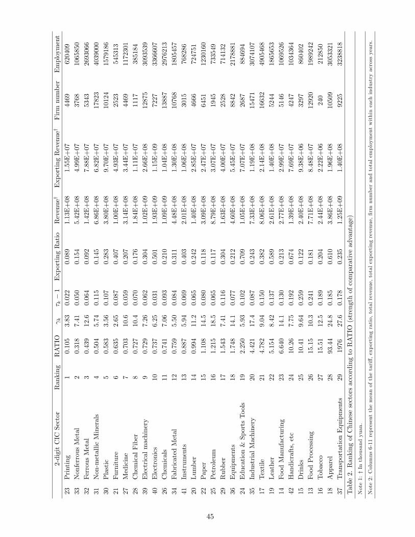
2-digitCICSector

Ranking

RATIO

k

� k�1

ExportingRatio

Revenuey

ExportingRevenuey

Firmnumber

Employment

23Printing

10.105

3.83

0.022

0.089

1.13E+08

1.55E+07

4469

620409

33NonferrousMetal

20.318

7.41

0.050

0.154

5.42E+08

4.99E+07

3768

1065850

32FerrousMetal

30.439

12.6

0.064

0.092

1.42E+08

7.88E+07

5343

2693066

31Non-metallicMinerals

40.504

5.74

0.115

0.145

6.86E+08

6.82E+07

17823

4039000

30Plastic

50.583

3.56

0.107

0.283

3.80E+08

9.70E+07

10124

1579186

21Furniture

60.635

2.65

0.087

0.407

1.00E+08

4.93E+07

2523

545313

27Medicine

70.703

10.6

0.059

0.207

3.14E+08

3.44E+07

4469

1172301

28ChemicalFiber

80.727

10.4

0.070

0.176

1.84E+08

1.11E+07

1117

385184

39Electricalmachinery

90.729

7.26

0.062

0.304

1.02E+09

2.66E+08

12875

3093539

40Electronics

100.737

6.25

0.031

0.501

1.93E+09

1.15E+09

7227

3366607

26Chemicals

110.741

7.06

0.093

0.210

1.09E+09

1.04E+08

13887

2976213

34FabricatedMetal

120.759

5.50

0.084

0.311

4.48E+08

1.30E+08

10768

1805457

41Instruments

130.887

5.94

0.069

0.403

2.01E+08

1.06E+08

3015

768286

20Lumber

140.994

11.2

0.065

0.242

1.40E+08

2.85E+07

4666

724751

22Paper

151.108

14.5

0.080

0.118

3.09E+08

2.47E+07

6451

1230160

25Petroleum

161.215

18.5

0.065

0.117

8.79E+08

3.07E+07

1945

733549

29Rubber

171.543

7.41

0.116

0.304

1.63E+08

4.00E+07

2528

714132

36Equipments

181.748

14.1

0.077

0.212

4.60E+08

5.45E+07

8842

2178881

24Education&SportsTools

192.250

5.93

0.102

0.709

1.05E+08

7.07E+07

2687

884694

35IndustrialMachinery

204.421

17.4

0.087

0.243

7.33E+08

1.19E+08

15471

3074107

17Textile

214.782

9.04

0.150

0.382

8.06E+08

2.14E+08

16632

4905468

19Leather

225.154

8.42

0.137

0.589

2.61E+08

1.40E+08

5244

1865653

14FoodManufacturing

236.640

14.1

0.130

0.213

2.77E+08

2.99E+07

5146

1069526

42Handicrafts,etc

2410.26

7.75

0.192

0.674

1.39E+08

7.69E+07

4247

1034364

15Drinks

2510.41

9.64

0.259

0.122

2.40E+08

9.38E+06

3297

860402

13FoodProcessing

2615.15

10.3

0.241

0.181

7.71E+08

8.48E+07

12920

1989242

16Tobacco

2715.51

12.5

0.189

0.204

2.44E+08

2.22E+06

240

212850

18Apparel

2893.44

24.8

0.185

0.610

3.86E+08

1.96E+08

10509

3053321

37TransportationEquipments

291976

27.6

0.178

0.235

1.25E+09

1.40E+08

9225

3238818

Table2.RankingofChinesesectorsaccordingtoRATIO(strengthofcomparativeadvantage)

Note1:yInthousandyuan.

Note2:Columns6-11representthemeanofthetari¤,exportingratio,totalrevenue,totalexportingrevenue,�rm

numberandtotalemploymentwithineachindustryacrossyears.

45