qsep studies in economics and population
TRANSCRIPT
RESEARCH INSTITUTE FOR QUANTITATIVE
STUDIES IN ECONOMICS AND POPULATIONQSEP
AGGREGATION AND OTHER BIASES IN THE CALCULATION OF CONSUMER ELASTICITIES
FOR MODELS OF ARBITRARY RANK
FRANK T. DENTONDEAN C. MOUNTAIN
QSEP Research Report No. 447
August 2011
Frank Denton is a QSEP Research Associate and faculty member in the Department ofEconomics, McMaster University. Dean Mountain is a faculty member of the McMasterMichael G. DeGroote School of Business and an associate member of the Department ofEconomics.
The Research Institute for Quantitative Studies in Economics and Population (QSEP) is aninterdisciplinary institute established at McMaster University to encourage and facilitatetheoretical and empirical studies in economics, population, and related fields. For furtherinformation about QSEP visit our web site http://socserv.mcmaster.ca/qsep or contact Secretary,QSEP Research Institute, Kenneth Taylor Hall, Room 426, McMaster University, Hamilton,Ontario, Canada, L8S 4M4, FAX: 905 521 8232, Email: [email protected]. The ResearchReport series provides a vehicle for distributing the results of studies undertaken by QSEPassociates. Authors take full responsibility for all expressions of opinion.
AGGREGATION AND OTHER BIASES IN THECALCULATION OF CONSUMER ELASTICITIES
FOR MODELS OF ARBITRARY RANK
FRANK T. DENTONDEAN C. MOUNTAIN
QSEP Research Report No. 447
Aggregation and Other Biases in the Calculation of
Consumer Elasticities for Models of Arbitrary Rank
Frank T. Denton and Dean C. Mountain*
McMaster University
Consumer-related policy decisions often require analysis of aggregate responses or mean elasticities. However, in practice these mean elasticities are seldom used. Mean elasticities can be approximated using aggregate data, but that introduces aggregation bias for full and compensated price elasticities, though interestingly not for expenditure elasticities. The biases corresponding to incorrect approximations of mean elasticities depend on the type of data (micro or aggregate), the type and rank of the model, and generalized measures of income inequality. These biases are distinct from the biases (already noted in the literature) when using aggregate data to estimate micro elasticites at mean income.
Keywords: Aggregate price and expenditure elasticities, aggregation bias, consumer demand, generalized measures of income inequality, income distribution
JEL Classification: D11, C43
_____________
*Email: [email protected]; [email protected] . Helpful suggestions and comments of Arthur Lewbel are greatly appreciated.
2
Aggregation and Other Biases in the Calculation
of Consumer Elasticities for Models of Arbitrary Rank
1. Introduction
Economic policy decisions frequently require the evaluation of aggregate
responses - the aggregate response of consumer expenditure on gasoline to a gasoline tax,
say, or the aggregate effect of an income supplement on the demand for rental housing.1
Such responses are often represented best in the form of aggregate elasticities - or mean
elasticities, since the two are the same. True mean elasticity formulas are seldom used,
though. Elasticities are often reported at mean or other income levels for models fitted to
micro data and elasticities calculated from aggregate data (and hence subject to
aggregation bias) are often interpreted as elasticities at mean income. But elasticities at
the mean are not the same as mean elasticities; they are approximations at best and fail to
take into account the characteristics of the income distribution. We derive in this paper
exact formulas for mean price and expenditure elasticities for models of arbitrary rank
and arbitrary income distribution. We derive also formulas for the biases resulting from
the use of elasticities at the mean to represent mean elasticities and from the use of
aggregate rather than micro data in the calculation of either. We then show what the
biases look like for four familiar consumer expenditure models. (The biases are
theoretical. They are illustrated numerically but the paper is not concerned with issues of
statistical estimation.)
Three types of elasticities are of interest: expenditure elasticities, full
(uncompensated) price elasticities, and compensated price elasticities. (Full price
elasticities may be of practical importance for policy forecasting - forecasting the revenue
yield of the gasoline tax, for example - while compensated price elasticities are of more
interest from a welfare point of view.) We consider three situations (in describing them 1 In their survey on how to account for heterogeneity in aggregation, Blundell and Stoker (2005) begin their discussion by emphasizing that “some of the most important questions in economics…concern economic aggregates.” Economics “is often concerned with…aggregate consumption and savings, market demand and supply, total tax revenues,… and so forth.” Moreover, Slottje (2008) points to the recent “experiment of the US government in pumping over $50 billion dollars into consumers’ hands to jump start the US economy in 2008” as an exemplification of “the importance of understanding aggregate consumer behavior and what does and does not impact it.”
3
we follow the frequent practice in the literature of using “income” as equivalent to total
expenditure, in references to the income distribution):
(1) Micro data are available and are used to calculate mean (or aggregate) elasticities.
(2) Micro data are available and are used to calculate elasticities at the mean of the
income distribution. The elasticities at the mean are then used as approximations to mean
elasticities.
(3) Only aggregate data are available (time series, say) and those are used to estimate the
underlying micro model and corresponding elasticities. The elasticities are interpreted as
if they were mean or “representative consumer” elasticities in the micro model, and
possibly used to represent the aggregate effects of a price or income change.2
We derive the formulas for calculating the mean elasticities in situation (1) and the biases
implicit in situations (2) and (3). The biases depend on the structure of the income
distribution, irrespective of whether micro data or aggregate data are used. But there is an
interesting exception: calculations of mean expenditure elasticities based on aggregate
data are unbiased; regardless of the income distribution there is no aggregation error.
2. Framework
Assume I commodities, indexed by i , K households, indexed by k , and a
common price vector ),...,,( 21 Ipppp = (sometimes referred to as the law of one price).
Household k spends ikx units of income to purchase 0>ikq units of commodity i , has
2In spite of the increased availability and obvious advantages of micro data sets it is still the case that aggregate data must often be used in estimating consumer demand models. Of 21 published articles surveyed by the present authors, 15 used aggregate data in the estimation of “almost ideal demand systems,” either AIDS or QUAIDS (Denton and Mountain, 2007). The reasons no doubt vary: lack of availability of micro data for a particular country or region, lack of sufficient commodity detail required for a particular purpose, or of observations on particular explanatory variables, the need to use time series available only at the aggregate level in order to estimate a model with dynamic properties, and so on. We note too that much of the attention given to elasticities calculated from aggregate data in the literature has focused on their use as estimates of underlying micro elasticities, much less on their use as estimates of aggregate elasticities, even though the latter are often of greater policy relevance.
4
total income (expenditure) kx , and thus an expenditure share k
ikik x
xw = . Now consider,
for some arbitrary R , the generic expenditure system
( ) ),...,2,1(,)(~1
0
Iipxfx
pcwR
rkr
k
riik == ∑
−
=
(1)
where ( ) ⎟⎟⎠
⎞⎜⎜⎝
⎛ −=
)()(
,pb
pdxfpxf k
rkr for a translated and deflated system, the )(~ pcri can be
interpreted as coefficients, conditional on p , and the functions )( pd and )( pb are
homogeneous of degree one.3 (Note that demographic, geographic, and other such
household characteristics commonly included as additional variables in expenditure
models can be accommodated in ic0~ (p) and )( pd .) The rank of the demand system is the
maximum number of dimensions spanned by the system’s Engle curves. Equation (1)
nests Gorman’s (1981) rank 3 rationally derived system, Lewbel’s (1989a) rank 4
rationally derived system, and Lewbel’s (2003) translated deflated income system. At the
level of specific applicable models it nests such well known ones as the translog
(Christensen, Jorgenson, and Lau, 1975), AIDS (Deaton and Muellbauer, 1980), and
QUAIDS (Banks, Blundell, and Lewbel, 1997). More generally, it is consistent with
many studies in which expenditure systems have been found to be well approximated by
finite (invariably low) order log-income polynomials. In the case of rank 2 and rank 3
polynomials in logarithms of deflated expenditures, such as translog, AIDS and
QUAIDS, equation (1) simplifies to
( )∑−
=
==1
0),...,2,1(ln)(
R
r
rkriik Iixpaw for 3,2=R (2)
3 To obtain this expenditure system, we could begin with
( )i
riri
R
rkrriik p
pcpcwhereIipxfpcq
)(~)(~~),...,2,1(,)(~~1
0===∑
−
=
5
by dropping the translation term )( pd and by setting r
kkkr pb
xpb
xpxf ⎥
⎦
⎤⎢⎣
⎡⎟⎟⎠
⎞⎜⎜⎝
⎛=
(ln
)(),(
and ( ) rjR
rjjiri pb
rjj
pcpbpa −−
=
−⎟⎟⎠
⎞⎜⎜⎝
⎛−
= ∑ )(ln()(~)()(1
. Here R is the rank of the system.
Reformulating k
kr
xpxf ),(
in equation (1) as a Taylor series expansion in kxln
around 0ln =kx ( 1=kx ), and using the notation rf to denote the function ),( pxf kr ,
results in
( ) ( ) ),...,2,1(ln|1ln!
1)(~10
1
0Iixf
xf
mpcw m
kx
rm
mk
rm
m
R
rriik
k
=⎟⎟⎠
⎞⎜⎜⎝
⎛−+
∂∂
==
∞
=
−
=∑∑ ,
with 000
0
lnf
xf
k
=∂
∂ .
With further regrouping of terms involving ( )mkxln , this can be further simplified to
( )∑∞
=
==0
),...,2,1(ln)(m
mkmiik Iixpcw (3)
where ( )1
1
0|1
ln!1)(~)(
=
−
=⎟⎟⎠
⎞⎜⎜⎝
⎛−+
∂
∂= ∑
kxr
mm
k
rmR
rrimi f
xf
mpcpc
The fact that equation (3) nests equation (2) can be seen by setting to zero all the
derivatives of order higher than 2.
Elasticities (the focus of this paper) are invariant to scalar transformations of the
units of measurement for income and prices. This allows us to simplify notation, without
loss of generality (and with no implications for how a model might actually be estimated
6
in practice), by introducing the normalization restrictions ipi ∀= ,1 , and 1=x
where ∑=
=K
k
k
Kx
x1
. Hereafter we write simply mic , if the context permits.
We now need an appropriate way of characterizing the income distribution. To
that end we write ∑=
=K
kkxX
1
, Xx
y kk = , and ,...).2,1,0()ln(ln
1=−= ∑
=
mxxyh mk
K
kkm
We
can interpret mh as a generalized measure of inequality (GMI) of order m . This is a
straightforward mathematical generalization of Theil’s (1967) measure of inequality,
which is obtained by setting 1=m , and which was inspired by Shannon’s (1948)
measure of information entropy. An arbitrary income distribution can then be
characterized by the sequence ,,, 210 hhh etc. (Note that 10 =h . Note too that 0=mh for
all 0>m when the distribution is uniform.) Invoking the normalization restriction 1=x
allows the simpler definition mk
K
kkm xyh )(ln
1∑=
= .
The GMIs provide a bridge from the micro specification of equation (3) to the
corresponding specification at the aggregate level. Let iX be aggregate expenditure on
commodity i by all households and let ∑=
==K
kkik
ii yw
XX
W1
be the aggregate expenditure
share. Then
∑∑ ∑∞
=
∞
= =
==00 1
)(lnm
mmim
mk
K
kkmii hcxycW (4)
For polynomials in logarithms of deflated expenditures defined in equation (2) for
3,2=R , the aggregate expenditure share is
∑∑ ∑−
=
−
= =
==1
0
1
0 1)(ln
R
rrri
R
r
rk
K
kkrii haxyaW (5)
7
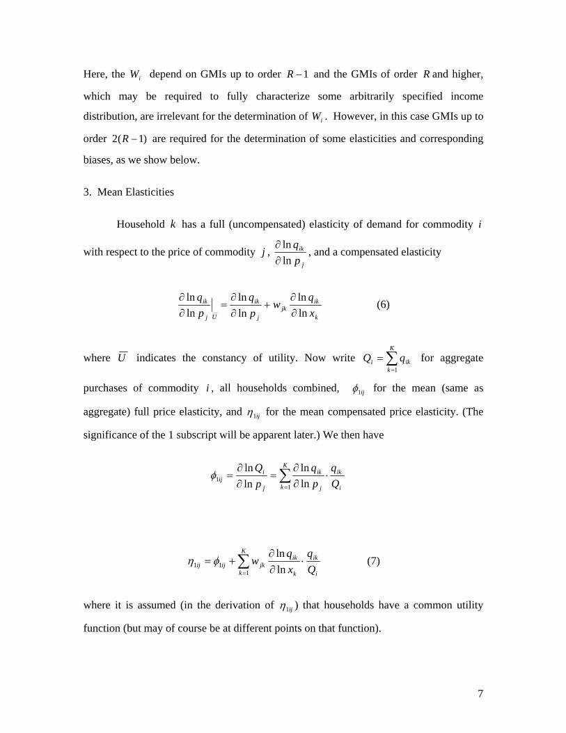
Here, the iW depend on GMIs up to order 1−R and the GMIs of order R and higher,
which may be required to fully characterize some arbitrarily specified income
distribution, are irrelevant for the determination of iW . However, in this case GMIs up to
order )1(2 −R are required for the determination of some elasticities and corresponding
biases, as we show below.
3. Mean Elasticities
Household k has a full (uncompensated) elasticity of demand for commodity i
with respect to the price of commodity j , j
ik
pq
lnln
∂∂
, and a compensated elasticity
k
ikjk
j
ik
Uj
ik
xq
wpq
pq
lnln
lnln
lnln
∂∂
+∂∂
=∂∂ (6)
where U indicates the constancy of utility. Now write ∑=
=K
kiki qQ
1
for aggregate
purchases of commodity i , all households combined, ij1φ for the mean (same as
aggregate) full price elasticity, and ij1η for the mean compensated price elasticity. (The
significance of the 1 subscript will be apparent later.) We then have
i
ikK
k j
ik
j
iij Q
qpq
pQ ∑
=
⋅∂∂
=∂∂
=1
1 lnln
lnln
φ
∑=
⋅∂∂
+=K
k i
ik
k
ikjkijij Q
qxq
w1
11 lnln
φη (7)
where it is assumed (in the derivation of ij1η ) that households have a common utility
function (but may of course be at different points on that function).
8
The expenditure elasticity for commodity i and for household k is k
ik
xq
lnln
∂∂
. To
derive a corresponding mean elasticity it is necessary to stipulate how a proportional
increase in aggregate income is shared among households. The most straightforward
assumption, and the one that we make, is that the proportional change is the same for all
households, so that 1lnln
=∂∂
Xxk for all .k 4 Writing i1ε for the mean expenditure
elasticity we then have
i
ikK
k k
ikk
ki
ik
ik
kK
k k
ik
i
ii Q
qxq
Xx
xX
qx
xq
QX
XQ ∑∑
==
⋅∂∂
=∂∂⋅⋅⋅⋅
∂∂
=⋅∂∂
=11
1 lnln
ε (8)
4. Calculations with Micro Data
Given an appropriate set of data for individual households and an expenditure
system defined by equation (3), price and expenditure elasticities can be calculated
directly, whatever the distribution of income. These elasticities are the correct ones for
evaluating aggregate effects. Elasticities at the mean of the income distribution can also
be calculated, either for their own value or as (biased) approximations to the mean
elasticities. We present the results of these calculations in the form of two theorems and a
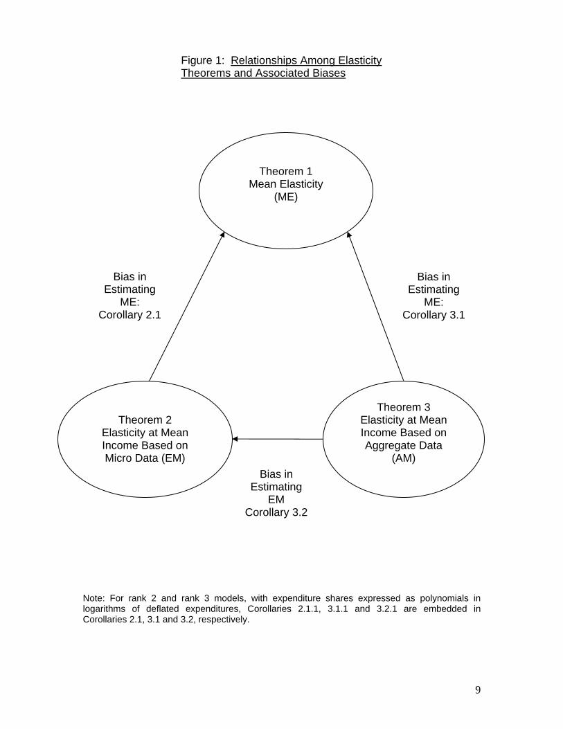
corollary. (All proofs are provided in Appendix A, both for this section and the next.)
Figure 1 provides a schematic illustration of the relationship among these two theorems
(theorems dealing with the use of micro data to calculate the elasticity at the mean of the
income distribution (EM), and the mean elasticity (ME)) and our third theorem, which is
concerned with estimating the elasticity at mean income based on aggregate data (AM).
The biases in using one of these elasticities (EM or AM) to estimate another (ME or EM),
as identified in the corollaries, are correspondingly labeled in the figure.
4 This assumption is consistent with what Lewbel (1989b, 1990) calls “mean scaling.”
9
Note: For rank 2 and rank 3 models, with expenditure shares expressed as polynomials in logarithms of deflated expenditures, Corollaries 2.1.1, 3.1.1 and 3.2.1 are embedded in Corollaries 2.1, 3.1 and 3.2, respectively.
Theorem 1
Mean Elasticity (ME)
Bias in Estimating
ME: Corollary 3.1
Bias in Estimating
ME: Corollary 2.1
Theorem 3 Elasticity at Mean Income Based on Aggregate Data
(AM)
Theorem 2
Elasticity at Mean Income Based on Micro Data (EM)
Figure 1: Relationships Among Elasticity Theorems and Associated Biases
Bias in Estimating
EM Corollary 3.2
10
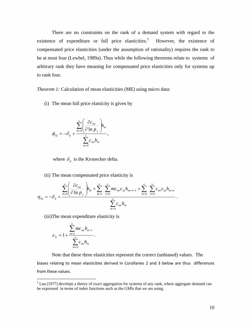
There are no constraints on the rank of a demand system with regard to the
existence of expenditure or full price elasticities.5 However, the existence of
compensated price elasticities (under the assumption of rationality) requires the rank to
be at most four (Lewbel, 1989a). Thus while the following theorems relate to systems of
arbitrary rank they have meaning for compensated price elasticities only for systems up
to rank four.
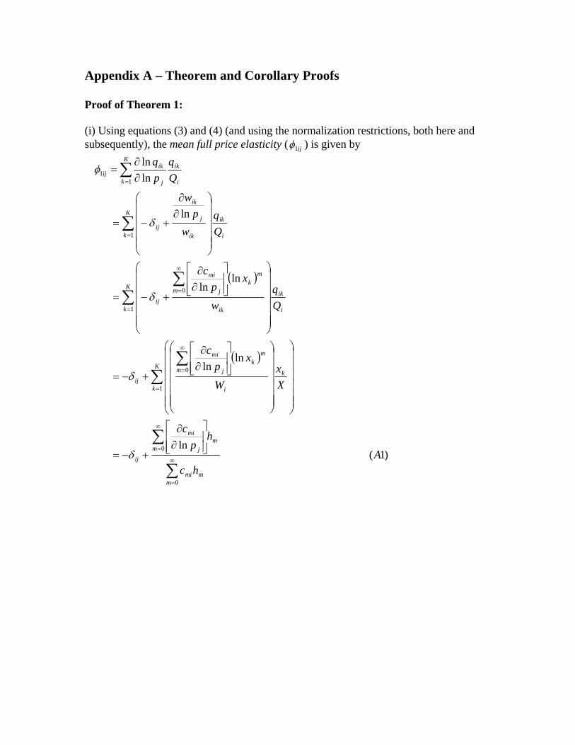
Theorem 1: Calculation of mean elasticities (ME) using micro data:
(i) The mean full price elasticity is given by
,ln
0
01
∑
∑∞
=
∞
=⎟⎟⎠
⎞⎜⎜⎝
⎛
∂∂
+−=
mmmi
mm
j
mi
ijij
hc
hp
c
δφ
where ijδ is the Kronecker delta.
(ii) The mean compensated price elasticity is
.ln
0
0001
101
∑
∑∑∑∑∑∞
=
∞
=+
∞
=
∞
=−+
∞
=
∞
=
++⎟⎟⎠
⎞⎜⎜⎝
⎛
∂∂
+−=
mmmi
nnmnjmi
mnnmnjmi
mmm
j
mi
ijij
hc
hcchcmchp
c
δη
(iii)The mean expenditure elasticity is
.1
0
11
1
∑
∑∞
=
−
∞
=+=
mmmi
mm
mi
i
hc
hmcε
Note that these three elasticities represent the correct (unbiased) values. The
biases relating to mean elasticities derived in Corollaries 2 and 3 below are thus differences
from these values. 5 Lau (1977) develops a theory of exact aggregation for systems of any rank, where aggregate demand can be expressed in terms of index functions such as the GMIs that we are using.
11
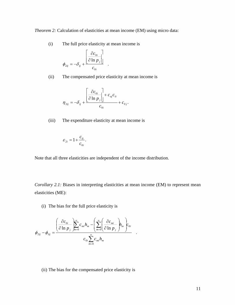
Theorem 2: Calculation of elasticities at mean income (EM) using micro data:
(i) The full price elasticity at mean income is
.ln
0
0
2i
j
i
ijij c
pc
⎥⎥⎦
⎤
⎢⎢⎣
⎡
∂∂
+−= δφ
(ii) The compensated price elasticity at mean income is
.ln
00
10
2 ji
iojj
i
ijij cc
ccp
c
+
+⎥⎥⎦
⎤
⎢⎢⎣
⎡
∂∂
+−= δη
(iii) The expenditure elasticity at mean income is
.10
12
i
ii c
c+=ε
Note that all three elasticities are independent of the income distribution.
Corollary 2.1: Biases in interpreting elasticities at mean income (EM) to represent mean
elasticities (ME):
(i) The bias for the full price elasticity is
.lnln
00
000
0
12
∑
∑∑∞
=
∞
=
∞
= ⎟⎟⎠
⎞⎜⎜⎝
⎛⎟⎟⎠
⎞⎜⎜⎝
⎛
∂∂
−⎟⎟⎠
⎞⎜⎜⎝
⎛
∂∂
=−
mmmii
im
mj
mi
mmmi
j
i
ijij
hcc
chp
chc
pc
φφ
(ii) The bias for the compensated price elasticity is
12
.ln
ln
00
0000
110
0100
0
12
∑
∑∑∑∑∑
∑
∞
=
∞
=+
∞
=
∞
=−+
∞
=
∞
=
∞
=
⎪⎪⎪
⎭
⎪⎪⎪
⎬
⎫
⎪⎪⎪
⎩
⎪⎪⎪
⎨
⎧
⎟⎟⎠
⎞⎜⎜⎝
⎛++⎟
⎟⎠
⎞⎜⎜⎝
⎛
∂∂
−⎟⎟⎠
⎞⎜⎜⎝
⎛+⎟⎟⎠
⎞⎜⎜⎝
⎛+
∂∂
=−
mmmii
in
nmnjmimn
nmnjmimm
mj
mi
mmmiiojij
j
i
ijij
hcc
chcchcmchp
c
hcccccp
c
ηη
(iii) The bias for the expenditure elasticity is
.
00
0 1101
12
∑
∑ ∑∞
=
∞
=
∞
=−−
=−
mmmii
m mmmiimmii
ii
hcc
hmcchccεε
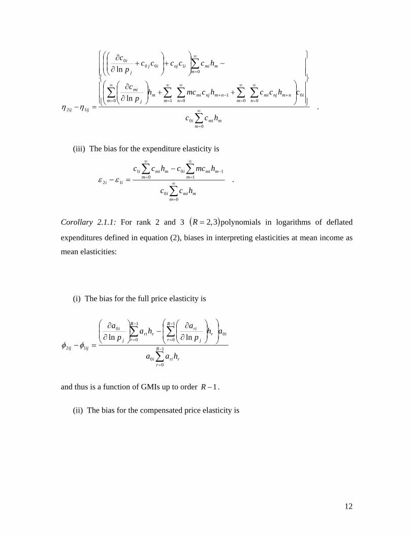
Corollary 2.1.1: For rank 2 and 3 ( )3,2=R polynomials in logarithms of deflated
expenditures defined in equation (2), biases in interpreting elasticities at mean income as
mean elasticities:
(i) The bias for the full price elasticity is
∑
∑∑−
=
−
=
−
= ⎟⎟⎠
⎞⎜⎜⎝
⎛⎟⎟⎠
⎞⎜⎜⎝
⎛
∂∂
−⎟⎟⎠
⎞⎜⎜⎝
⎛
∂∂
=− 1
00
0
1
0
1
0
0
12
lnlnR
rrrii
i
R
rr
j
riR
rrri
j
i
ijij
haa
ahp
aha
pa
φφ
and thus is a function of GMIs up to order 1−R .
(ii) The bias for the compensated price elasticity is
13
∑
∑∑∑∑∑
∑
−
=
−
=+
−
=
−
=−+
−
=
−
=
−
=
⎪⎪⎪
⎭
⎪⎪⎪
⎬
⎫
⎪⎪⎪
⎩
⎪⎪⎪
⎨
⎧
⎟⎟⎠
⎞⎜⎜⎝
⎛++⎟
⎟⎠
⎞⎜⎜⎝
⎛
∂∂
−⎟⎟⎠
⎞⎜⎜⎝
⎛+⎟
⎟⎠
⎞⎜⎜⎝
⎛+
∂∂
=− 1
00
0
1
0
1
0
1
01
1
1
1
0
1
0100
0
12
ln
ln
R
rrrii
i
R
ssrsjri
R
r
R
ssrsjri
R
r
R
rr
j
ri
R
rrriiojij
j
i
ijij
haa
ahaaharahp
a
haaaaap
a
ηη and thus is a
function of GMIs up to order )1(2 −R .
(iii) The bias for the expenditure elasticity is
∑
∑ ∑−
=
−
=
−
=−−
=− 1
00
1
0
1
1101
12 R
rrrii
R
r
R
rrriirrii
ii
haa
hraahaaεε
and thus is a function of GMIs up to order 1−R .
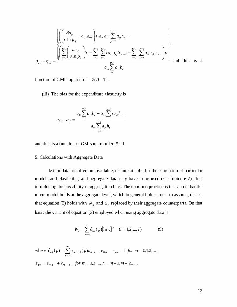
5. Calculations with Aggregate Data
Micro data are often not available, or not suitable, for the estimation of particular
models and elasticities, and aggregate data may have to be used (see footnote 2), thus
introducing the possibility of aggregation bias. The common practice is to assume that the
micro model holds at the aggregate level, which in general it does not – to assume, that is,
that equation (3) holds with ikw and kx replaced by their aggregate counterparts. On that
basis the variant of equation (3) employed when using aggregate data is
[ ] ),...,2,1(ln)(ˆ0
IixpcW m
mmii == ∑
∞
=
(9)
where ∑∞
=−=
mnmnnimnmi hpcepc )()(ˆ , ,...2,1,010 === mforee mmm ,
,...2,1,...,2,11,11, ++==+= −−− mmnmforeee nmnmmn .
14
The associated full price, compensated price, and expenditure elasticities for this
model are obtained by calculating
,lnln
,lnln
33Uj
iij
j
iij p
QpQ
∂∂
=∂∂
= ηφ and XQi
i lnln
3 ∂∂
=ε ,
where ijijij W 333 εφη += . (10).
The formulas for these calculations using aggregate data are stated in the following
theorem:
Theorem 3: Calculation of elasticities at mean income using aggregate data (AM), based
on equation (9):
(i) The full price elasticity is
(ii) The compensated price elasticity is
.ln
0
110
00
0
3
∑
∑∑∑∞
=
∞
=−
∞
=
∞
=
++∂∂
+−=
mmmi
mmmij
mmnminj
nj
i
ijij
hc
hcmchhccp
c
δη
(iii) The expenditure elasticity is
.1
0
11
3
∑
∑∞
=
∞
=−
+=
mmmi
mmmi
i
hc
hmcε
.ln
0
11
1
0
3
∑
∑∑∞
=
∞
=−
∞
=
−∂∂
+−=
mmmi
nn
mnjmimj
i
ijij
hc
hhcmcp
c
δφ
15
If the formulas in Theorem 3 are applied, and the results are interpreted as true
mean elasticities, the biases are as given in Corollary 3.1. If on the other hand the results
are interpreted as elasticities at mean income the biases are as given in Corollary 3.2.6
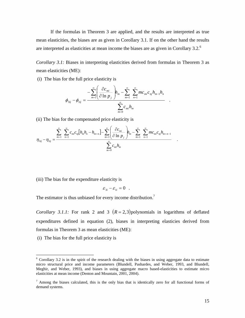
Corollary 3.1: Biases in interpreting elasticities derived from formulas in Theorem 3 as
mean elasticities (ME):
(i) The bias for the full price elasticity is
.ln
0
1 11
113
∑
∑ ∑∑∞
=
∞
=
∞
=−
∞
=
−⎟⎟⎠
⎞⎜⎜⎝
⎛
∂∂
−
=−
mmmi
mn
nmnjmi
mm
j
mi
ijij
hc
hhcmchp
c
φφ
(ii) The bias for the compensated price elasticity is
[ ].
ln
0
111111
13
∑
∑∑∑∑∑∞
=
−+
∞
=
∞
=
∞
=+
∞
=
∞
=
−⎟⎟⎠
⎞⎜⎜⎝
⎛
∂∂
−−
=−
mmmi
nmn
njmimm
mj
minmnm
nnjmi
mijij
hc
hcmchp
chhhccηη
(iii) The bias for the expenditure elasticity is
013 =− ii εε .
The estimator is thus unbiased for every income distribution.7
Corollary 3.1.1: For rank 2 and 3 ( )3,2=R polynomials in logarithms of deflated
expenditures defined in equation (2), biases in interpreting elasticies derived from
formulas in Theorem 3 as mean elasticities (ME):
(i) The bias for the full price elasticity is
6 Corollary 3.2 is in the spirit of the research dealing with the biases in using aggregate data to estimate micro structural price and income parameters (Blundell, Pashardes, and Weber, 1993, and Blundell, Meghir, and Weber, 1993), and biases in using aggregate macro based-elasticities to estimate micro elasticities at mean income (Denton and Mountain, 2001, 2004). 7 Among the biases calculated, this is the only bias that is identically zero for all functional forms of demand systems.
16
.ln
1
0
1
1
1
11
1
1
13
∑
∑ ∑∑−
=
−
=
−
=−
−
=
−⎟⎟⎠
⎞⎜⎜⎝
⎛
∂∂
−
=−R
rrri
R
rs
R
srsjri
R
rr
j
ri
ijij
ha
hharahp
a
φφ ,
and thus is a function of GMIs up to order 1−R .
(ii) The bias for the compensated price elasticity is
[ ].
ln1
0
1
11
1
1
1
1
1
1
1
1
13
∑
∑∑∑∑∑−
=
−
=−+
−
=
−
=+
−
=
−
=
−⎟⎟⎠
⎞⎜⎜⎝
⎛
∂∂
−−
=− R
rrri
R
ssrsjri
R
r
R
rr
j
risrsr
R
ssjri
R
r
ijij
ha
harahp
ahhhaa
ηη
and thus is a function of GMIs up to order )1(2 −R .
(iii) The bias for the expenditure elasticity is
013 =− ii εε .
The estimator is thus unbiased for every income distribution.
Corollary 3.2: Biases in interpreting elasticies derived from formulas in Theorem 3 as
elasticities at mean income (EM):
(i) The bias for the full price elasticity is
.ln
00
11
10
00
0
23
∑
∑∑∑∞
=
∞
=−
∞
=
∞
=
−⎟⎠
⎞⎜⎝
⎛−
∂∂
=−
mmmii
nn
mnjmim
im
mmiij
i
ijij
hcc
hhcmcchccp
c
φφ
(ii) The bias for the compensated price elasticity is
17
.lnln
00
0001
0
0 110
0
00
23
∑
∑∑ ∑∑∞
=
∞
=
∞
=
∞
=−
∞
= ⎪⎭
⎪⎬⎫
⎪⎩
⎪⎨⎧
⋅⎥⎥⎦
⎤
⎢⎢⎣
⎡++
∂∂
−⎥⎥⎦
⎤
⎢⎢⎣
⎡++
∂∂
⋅
=−
mmmii
mmmiijioj
j
i
m mmmijmnminj
nj
ii
ijij
hcc
hcccccp
chcmchhcc
pc
c
ηη
(iii) The bias for the expenditure elasticity is
.
00
01
110
23
∑
∑∑∞
=
∞
=
∞
=− −
=−
mmmii
mmmii
mmmii
ii
hcc
hcchmccεε
Corollary 3.2.1: For rank 2 and 3 ( )3,2=R polynomials in logarithms of deflated
expenditures defined in equation (2), biases in interpreting elasticities derived from
formulas in Theorem 3 as elasticities at mean income (EM):
(i) The bias for the full price elasticity is
∑
∑∑∑−
=
−
=−
−
=
−
=
−⎟⎠
⎞⎜⎝
⎛−
∂∂
=− 1
00
1
11
1
10
1
00
0
23
lnR
rrrii
s
R
srsjri
R
ri
R
rrrii
j
i
ijij
haa
hharaahaap
a
φφ
and thus is a function of GMIs up to order 1−R .
(ii) The bias for the compensated price elasticity is
18
∑
∑∑ ∑∑−
=
−
=
−
=
−
=−
−
= ⎪⎭
⎪⎬⎫
⎪⎩
⎪⎨⎧
⋅⎥⎥⎦
⎤
⎢⎢⎣
⎡++
∂∂
−⎥⎥⎦
⎤
⎢⎢⎣
⎡++
∂∂
⋅
=− 1
00
1
0001
01
0
1
110
1
0
00
23
lnlnR
rrrii
R
rrriijioj
j
iR
r
R
rrrijrsrisj
R
sj
ii
ijij
haa
haaaaap
aharahhaa
pa
a
ηη
and thus is a function of GMIs up to order 1−R .
(iii) The bias for the expenditure elasticity is
∑
∑∑−
=
−
=
−
=− −
=− 1
00
1
01
1
110
23 R
rrrii
R
rrrii
R
rrrii
ii
haa
haahraaεε
and thus is a function of GMIs up to order 1−R .
All of the biases in Corollaries 3.1 and 3.2 are (in general) nonzero, with the
exception of the expenditure elasticity bias in Corollary 3.1, where aggregate data are
used to estimate the mean elasticity, and the bias is zero. The notion of a “representative
consumer” is often invoked to justify the use of aggregate data. For the expenditure
elasticity the representative consumer turns out in fact to be a household with mean
elasticity, whatever the rank of the system and the distribution of income. For the price
elasticities, though, that is not the case.
6. Illustrations
Four models of applied demand systems ranging from rank 2 to rank 4 that are
familiar in the literature are the translog (TLOG), the linear Almost Ideal Demand
System (AIDS), the quadratic extension of the linear system (QUAIDS), and Lewbel’s
rank 4 demand system, which we shall refer to as L4. TLOG and AIDS are rank 2
systems, QUAIDS is a rank 3 system. We use these four models to illustrate the biases
discussed above.
19
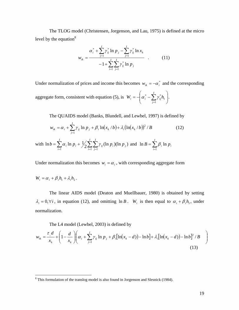
The TLOG model (Christensen, Jorgenson, and Lau, 1975) is defined at the micro
level by the equation8
∑∑
∑ ∑
= =
= =
+−
−+= I
i
I
jjij
I
j
I
jkijjiji
ik
p
xpw
1 1
*
1 1
***
ln1
lnln
γ
γγα . (11)
Under normalization of prices and income this becomes *iikw α−= and the corresponding
aggregate form, consistent with equation (5), is ⎟⎟⎠
⎞⎜⎜⎝
⎛−−= ∑
=1
1
** hWI
jijii γα .
The QUAIDS model (Banks, Blundell, and Lewbel, 1997) is defined by
( ) ( )( ) Bbxbxpw k
I
jikijijiik //ln/lnln 2
1∑=
+++= λβγα (12)
with ∑ ∑∑= = =
+=I
i
I
i
I
jjiijii pppb
1 1 1
))(ln(ln21lnln γα and ∑
=
=I
iii pB
1lnln β
Under normalization this becomes iiw α= , with corresponding aggregate form
21 hhW iiii λβα ++= .
The linear AIDS model (Deaton and Muellbauer, 1980) is obtained by setting
ii ∀= ,0λ , in equation (12), and omitting Bln . iW is then equal to 1hii βα + , under
normalization.
The L4 model (Lewbel, 2003) is defined by
( )[ ] ( )[ ] ⎟⎟⎠
⎞⎜⎜⎝
⎛−−+−−++⎟⎟
⎠
⎞⎜⎜⎝
⎛−+= ∑
=
Bbdxbdxpxd
xd
w k
I
jikijiji
kkik
i /ln)lnln)lnln1 2
1
λβγατ
(13)
8 This formulation of the translog model is also found in Jorgenson and Slesnick (1984).
20
with ∑ ∑∑= = =
++=I
i
I
i
I
jjiijii pppb
1 1 10 ))(ln(ln2
1lnln γαα , ∏=
=I
ii
ipd1
0τρ and
∑=
=I
iii pB
1
lnln β .9 Note that L4 nests QUAIDS ( Iiforand i ,...,2,1000 === τρ ) and
hence AIDS ( ,0=iλ additionally, for Ii ,...,2,1= ).
With normalization, equation (13) becomes ( ) iiiw αρρτ 00 1−+= . 10 In the
form of equation (3), the Taylor series expansion of equation (13) is
( )∑=
=+=3
0
),...,2,1(ln)(m
mkmiik Iiminorderhigheroftermsxpcw (14)
with
( ) ( )[ ] ( )[ ] ,/ln)1lnln)1lnln1)( 2
1⎟⎟⎠
⎞⎜⎜⎝
⎛−−+−−++−+= ∑
=
BbdbdpddpcI
jiijijioi i
λβγατ
( )[ ] ( )[ ]
( )[ ] ,ln)1ln2
/ln)1lnln)1lnln)( 2
11
bdB
Bbdbdpddpc
i
i
I
jiijijiii
−−
++⎟⎟⎠
⎞⎜⎜⎝
⎛−−+−−+++−= ∑
=
λ
βλβγατ
( )[ ] ( )[ ]
( )[ ] ,)1(
2ln)1ln21
/ln)1lnln)1lnln21)( 2
12
⎥⎦
⎤−
+⎟⎠⎞
⎜⎝⎛ −−+
−
⎢⎢⎣
⎡+⎟⎟
⎠
⎞⎜⎜⎝
⎛−−+−−++−= ∑
=
dBbd
Bdd
Bbdbdpddpc
iii
I
jiijijiii
λλβ
λβγατ
9 Two small typos appear in Lewbel’s (2003) original paper. The corrected version of the model can be found in Lewbel (2004). The demand system in equation (13) is the correct version. 10 Without loss of generality, part of the normalization for the L4 demand system is ( )00 1ln ρα −= .
21
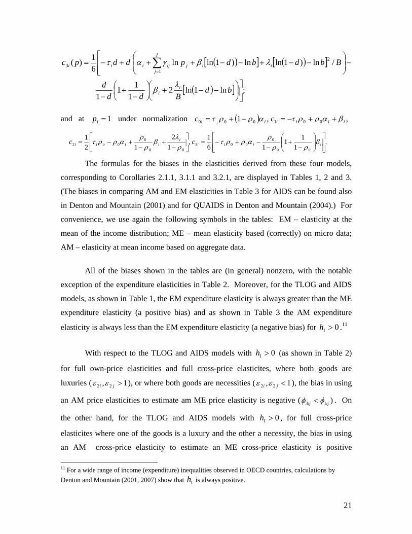
and at 1=ip under normalization ( ) ,,1 001000 iiiiii cci
βαρρταρρτ ++−=−+=
.1
1116
1,1
212
1
00
0003
00
002
⎥⎥⎦
⎤
⎢⎢⎣
⎡⎟⎟⎠
⎞⎜⎜⎝
⎛−
+−
−+−=⎥⎦
⎤⎢⎣
⎡−
+−
+−= iiiii
iioii cc βρρ
ραρρτ
ρλ
βρ
ραρρτ
The formulas for the biases in the elasticities derived from these four models,
corresponding to Corollaries 2.1.1, 3.1.1 and 3.2.1, are displayed in Tables 1, 2 and 3.
(The biases in comparing AM and EM elasticities in Table 3 for AIDS can be found also
in Denton and Mountain (2001) and for QUAIDS in Denton and Mountain (2004).) For
convenience, we use again the following symbols in the tables: EM – elasticity at the
mean of the income distribution; ME – mean elasticity based (correctly) on micro data;
AM – elasticity at mean income based on aggregate data.
All of the biases shown in the tables are (in general) nonzero, with the notable
exception of the expenditure elasticities in Table 2. Moreover, for the TLOG and AIDS
models, as shown in Table 1, the EM expenditure elasticity is always greater than the ME
expenditure elasticity (a positive bias) and as shown in Table 3 the AM expenditure
elasticity is always less than the EM expenditure elasticity (a negative bias) for 01 >h .11
With respect to the TLOG and AIDS models with 01 >h (as shown in Table 2)
for full own-price elasticities and full cross-price elasticites, where both goods are
luxuries ( 1, 22 >ji εε ), or where both goods are necessities ( 1, 22 <ji εε ), the bias in using
an AM price elasticities to estimate am ME price elasticity is negative ( )13 ijij φφ < . On
the other hand, for the TLOG and AIDS models with 01 >h , for full cross-price
elasticites where one of the goods is a luxury and the other a necessity, the bias in using
an AM cross-price elasticity to estimate an ME cross-price elasticity is positive
11 For a wide range of income (expenditure) inequalities observed in OECD countries, calculations by Denton and Mountain (2001, 2007) show that 1h is always positive.
( )[ ] ( )[ ]
( )[ ] ;ln1ln21
111
/ln)1lnln)1lnln61)( 2
13
⎥⎦
⎤⎟⎠⎞
⎜⎝⎛ −−+⎟⎠⎞
⎜⎝⎛
−+
−
⎢⎢⎣
⎡−⎟⎟
⎠
⎞⎜⎜⎝
⎛−−+−−+++−= ∑
=
bdBdd
d
Bbdbdpddpc
ii
I
jiijijiii
λβ
λβγατ
22
( ).13 ijij φφ > In all of these situations, the larger is the expenditure inequality (the larger is
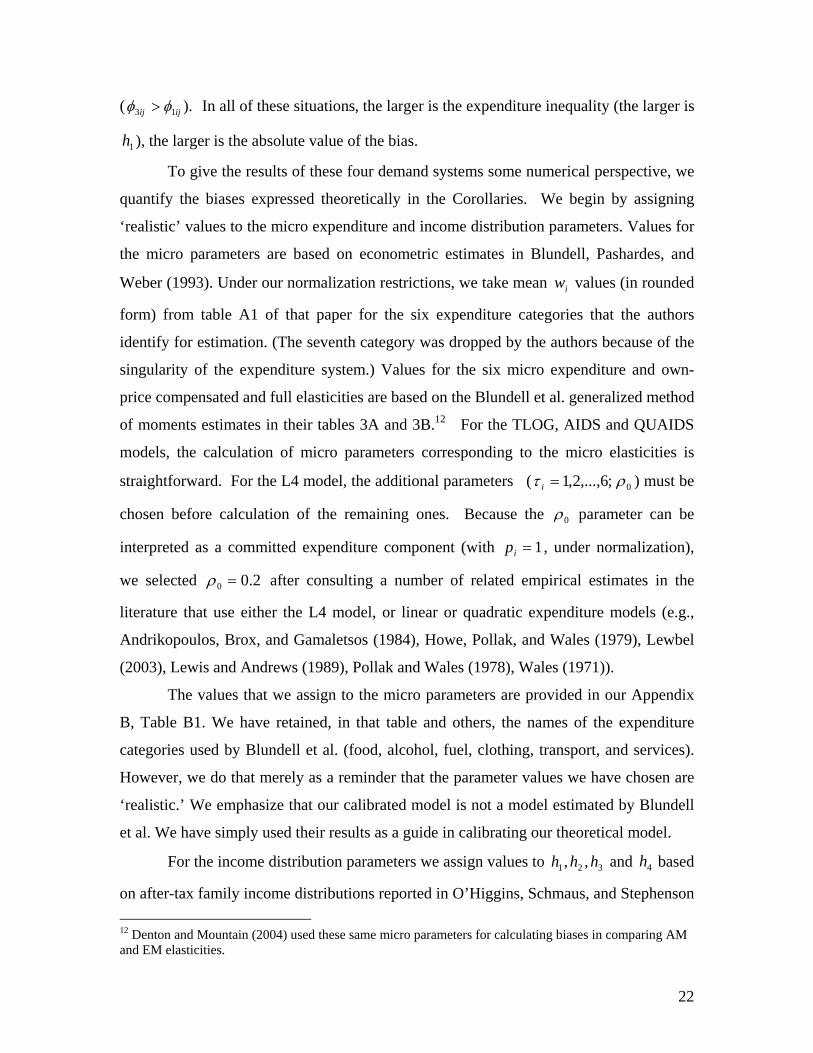
1h ), the larger is the absolute value of the bias.
To give the results of these four demand systems some numerical perspective, we
quantify the biases expressed theoretically in the Corollaries. We begin by assigning
‘realistic’ values to the micro expenditure and income distribution parameters. Values for
the micro parameters are based on econometric estimates in Blundell, Pashardes, and
Weber (1993). Under our normalization restrictions, we take mean iw values (in rounded
form) from table A1 of that paper for the six expenditure categories that the authors
identify for estimation. (The seventh category was dropped by the authors because of the
singularity of the expenditure system.) Values for the six micro expenditure and own-
price compensated and full elasticities are based on the Blundell et al. generalized method
of moments estimates in their tables 3A and 3B.12 For the TLOG, AIDS and QUAIDS
models, the calculation of micro parameters corresponding to the micro elasticities is
straightforward. For the L4 model, the additional parameters ( 0;6,...,2,1 ρτ =i ) must be
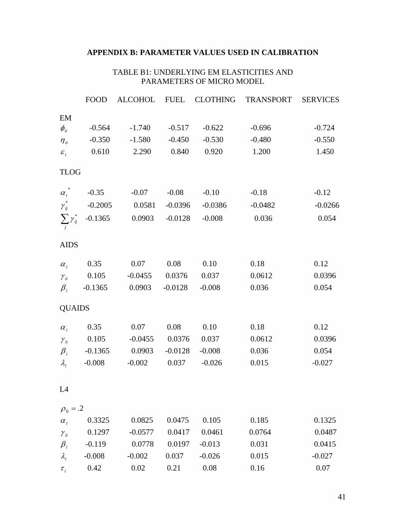
chosen before calculation of the remaining ones. Because the 0ρ parameter can be
interpreted as a committed expenditure component (with 1=ip , under normalization),
we selected 2.00 =ρ after consulting a number of related empirical estimates in the
literature that use either the L4 model, or linear or quadratic expenditure models (e.g.,
Andrikopoulos, Brox, and Gamaletsos (1984), Howe, Pollak, and Wales (1979), Lewbel
(2003), Lewis and Andrews (1989), Pollak and Wales (1978), Wales (1971)).
The values that we assign to the micro parameters are provided in our Appendix
B, Table B1. We have retained, in that table and others, the names of the expenditure
categories used by Blundell et al. (food, alcohol, fuel, clothing, transport, and services).
However, we do that merely as a reminder that the parameter values we have chosen are
‘realistic.’ We emphasize that our calibrated model is not a model estimated by Blundell
et al. We have simply used their results as a guide in calibrating our theoretical model.
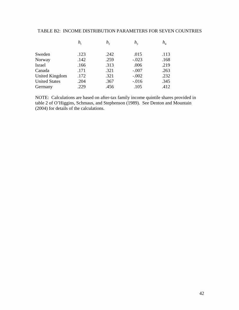
For the income distribution parameters we assign values to 321 ,, hhh and 4h based
on after-tax family income distributions reported in O’Higgins, Schmaus, and Stephenson 12 Denton and Mountain (2004) used these same micro parameters for calculating biases in comparing AM and EM elasticities.
23
(1989, table 2). Values were calculated for seven OECD countries, reflecting a wide
range of income distributions. The calculated values for 4321 ,, handhhh are provided in
Table B2 of Appendix B. For the L4 model our estimates of biases are based on
numerical approximations, where we made use of sh' up to 4h .
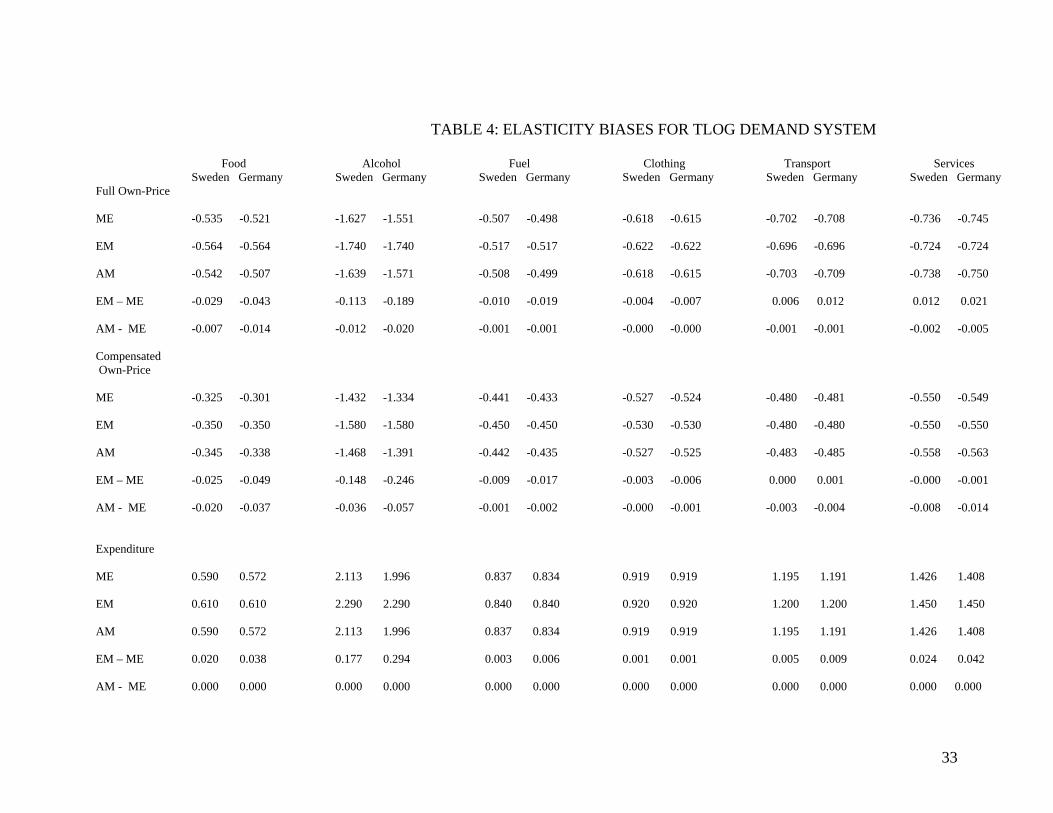
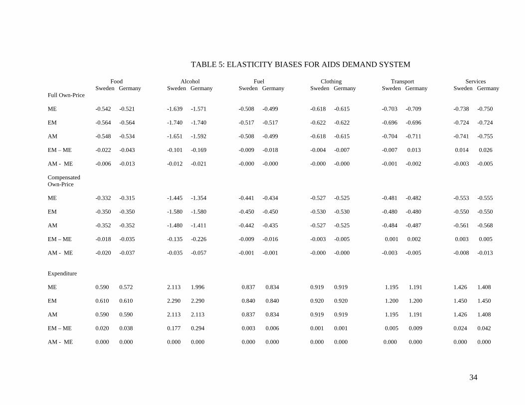
With the underlying micro parameters, we then calculated the biases reported in
Tables 1, 2 and 3 for countries with the least and greatest inequality of income
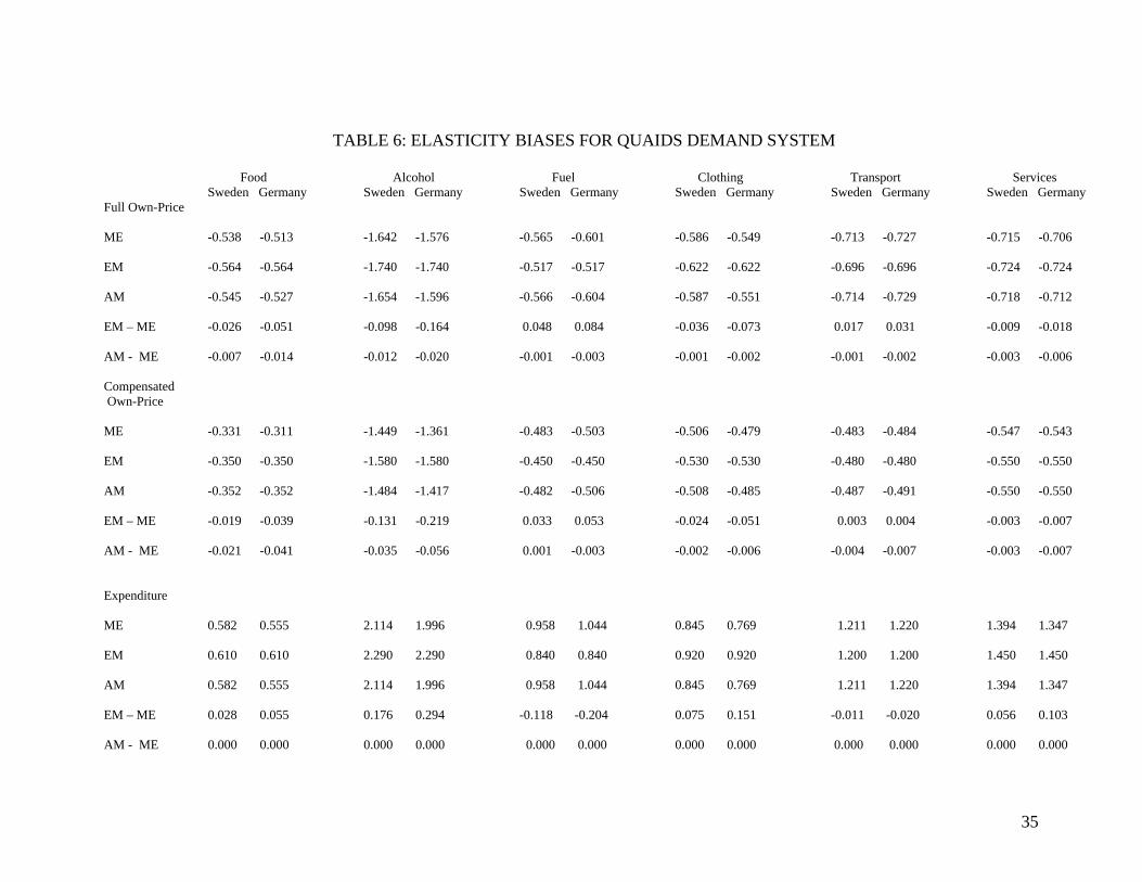
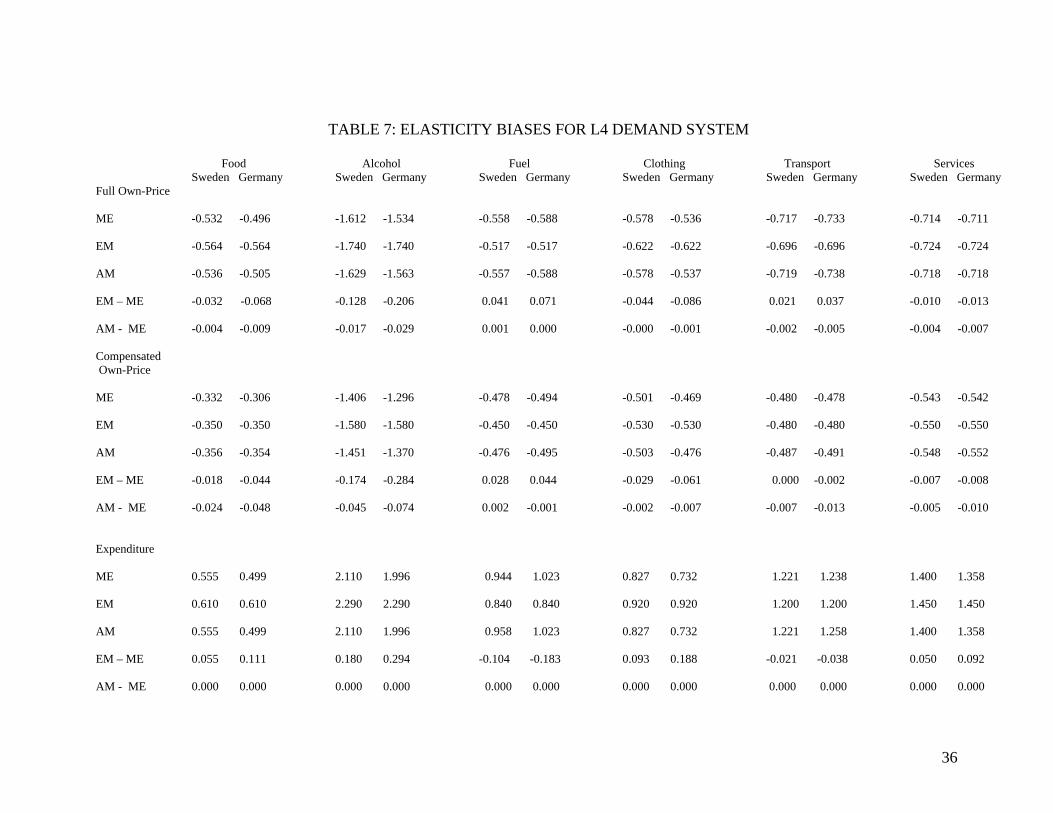
distribution, Sweden and Germany. Tables 4, 5, 6 and 7 report the corresponding mean
elasticities (ME), the micro elasticity calculated at the mean of the income distribution
(EM), and the elasticity at mean income based on aggregate data (AM) for all four
models. Biases in estimating ME with either EM or AM elasticity are calculated. This is
done for full own-price elasticities, compensated own-price elasticities and expenditure
elasticities.
The results are similar across all four models. The main conclusions are as
follows. Not unexpectedly, the greater the income inequality, the greater is the bias.
(The biases for Sweden are generally smaller than those for Germany.) Furthermore, the
greater the departure of the expenditure elasticity from one, the greater is the bias. For
example, for food and alcohol, with EMs of 0.61 and 2.29, respectively, the biases are
relatively large. This is in contrast with the results for clothing, with an EM of 0.92.
Although not always, generally, in estimating the ME the AM does a better job than the
EM. In terms of absolute size, the expenditure elasticity bias tends to be larger than the
full price and compensated price elasticity biases.
For the L4 model we also tried different values of 0ρ to investigate the sensitivity
of the results to that parameter’s value. When we changed the value of 0ρ from 0.2 to
0.5, we found the biases in the price elasticities to be only slightly larger. However, we
did find some much larger biases involving expenditure elasticities (e.g., MEEM −
biases are 0.113 and 0.235 for food in Sweden and Germany with 5.00 =ρ , compared
with 0.055 and 0.111 for 2.00 =ρ ).
24
7. Conclusion
We began this paper by noting that consumer-related policy decisions frequently
require the evaluation of aggregate responses, often in the form of mean price or
expenditure elasticities. Such elasticitities can be derived from a properly specified model
fitted to micro data, but in practice that is seldom done. They can be approximated from a
model fitted to aggregate data, but the approximation introduces the possibility of
aggregation bias in the calculation of price elasticities, though interestingly not in the
calculation of expenditure elasticities. We provide in this paper formulas for the correct
calculation of mean elasticities – expenditure and both full and compensated price
elasticities – and the corresponding biases when incorrect formulas are used. The correct
formulas and the biases depend in general on the type of data (micro or aggregate), the
type of model being estimated, the rank of the model, and the characteristics of the
income distribution.
We have quantified the range of biases for familiar demand systems. The
empirical results are robust in that the estimated biases are of the same order of
magnitude, regardless of the functional form. Whether we use AM or EM elasticities to
estimate the ME elasticity, the biases increase as the income inequality grows and as the
underlying expenditure elasticities depart from one. Generally, the AM elasticity
performs a better job than the EM elasticity in estimating ME.
25
References Andrikopoulos, A.A., J.A. Brox, and T. Gamaletsos (1984): Forecasting Canadian
Consumption Using the Dynamic Generlized Linear Expenditure System (DGLES),” Applied Economics, 16, 839-853.
Banks, J., R. Blundell, and A. Lewbel (1997): “Quadratic Engel Curves and Consumer
Demand,” Review of Economics and Statistics, 79, 527-539. Blundell, R., C. Meghir, and G. Weber (1993): “Aggregation and Consumer Behaviour:
Some Recent Results,” Ricerche Economiche, 47, 235-252. Blundell, R., P. Pashardes, and G. Weber (1993): “What Do We Learn About Consumer
Demand Patterns from Micro Data?” American Economic Review, 83, 570-597. Blundell, R., and T.M. Stoker (2005): “Heterogeneity and Aggregation,” Journal of
Economic Literature, 43, 347-391.
Christensen, L.R., D.W. Jorgenson, and L.J. Lau (1975): “Transcendental Logarithmic Utility Functions,” American Economic Review, 65, 367-383.
Deaton, A., and J. Muellbauer (1980): “An Almost Ideal Demand System,” American
Economic Review, 70, 312-326. Denton, F.T., and D.C. Mountain (2001): “Income Distribution and
Aggregation/Disaggregation Biases in the Measurement of Consumer Demand Elasticities,” Economics Letters, 21-28.
Denton, F.T., and D.C. Mountain (2004): “Aggregation Effects on Price and Expenditure
Elasticities in a Quadratic Almost Ideal Demand System,” Canadian Journal of Economics, 37, 613-628.
Denton, F.T., and D.C. Mountain (2011): “Exploring the Effects of Aggregation Error in the Estimation of Consumer Demand Elasticities,” Economic Modelling, 1747-1755.
Gorman, W.M. (1981): “Some Engel Curves,” in Essays in the Theory and Measurement
of Consumer Behaviour in Honor of Sir Richard Stone, ed. by A. Deaton. Cambridge, U.K.: Cambridge University Press, 7-29.
Howe, H., R.A. Pollak, and T.J. Wales (1979): “Theory and Time Series Estimation of
the Quadratic Expenditure System,” Econometrica, 47, 1231-1247.
26
Jorgenson, D.W. and D.T. Slesnick (1984): “Inequality in the Distribution of Individual Welfare,” in Advances in Econometrics, ed. by R.L. Basmann and G.F. Rhodes, Jr. Greenwich, Connecticut: JAI Press Inc., Vol. 3, 67-130.
Lau, L.J. (1977): “Existence Conditions for Aggregate Demand Functions: The Case of Multiple Indexes,” Technical report no. 248, Stanford, CA: Institute for Mathematical Studies in the Social Sciences, Stanford University
Lewbel, A. (1989a): “A Demand System Rank Theorem,” Econometrica, 57, 701-705. Lewbel, A. (1989b): “Exact Aggregation and a Representative Consumer,” Quarterly
Journal of Economics, 104, 621-633. Lewbel, A. (1990): “Income Distribution Movements and Aggregate Money Illusion,”
Journal of Econometrics, 43, 35-42. Lewbel, A. (2003): “A. Rational Rank Four Demand System,” Journal of Applied
Econometrics, 18, 127-135.
Lewbel, A. (2004): “A. Rational Rank Four Demand System (corrected version),” http://www2.bc.edu/~lewbel/rank4fix.pdf.
Lewis, P., and N. Andrews (1989): “Household Demand in China,” Applied Economics,
21, 793-807.
O’Higgins, M., G. Schmaus, and G. Stephenson (1989): “Income Distribution and Redistribution: a Microdata Analysis for Seven Countries,” Review of Income and
Wealth, 35, 107–131
Pollak, R.A., and T.J. Wales (1978): “Estimation of Complete Demand Systems from Household Budget Data: The Linear and Quadratic Expenditure Systems,” American Economic Review, 68, 348-359.
Shannon, C.E. (1948): “A Mathematical Theory of Communication,” Bell System
Technical Journal, 27, 379-423. Slottje, D. (2008): “Estimating Demand Systems and Measuring Consumer Preferences,”
Journal of Econometrics, 147, 207-209. Theil, H. (1967): Economics and Information Theory. Chicago: Rand McNally and
Company.
Wales, T.J. (1971): “A Generalized Linear Expenditure Model of the Demand for Non- Durable Goods in Canada,” Canadian Journal of Economics, 4, 471-484.
27
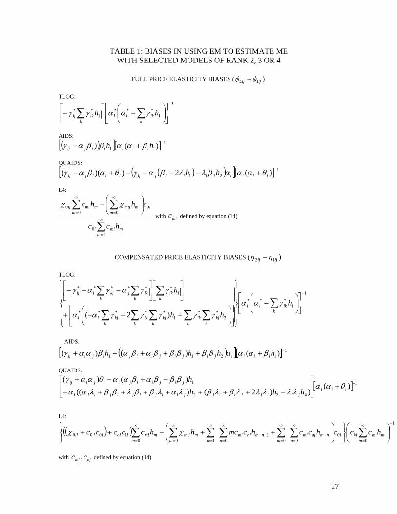
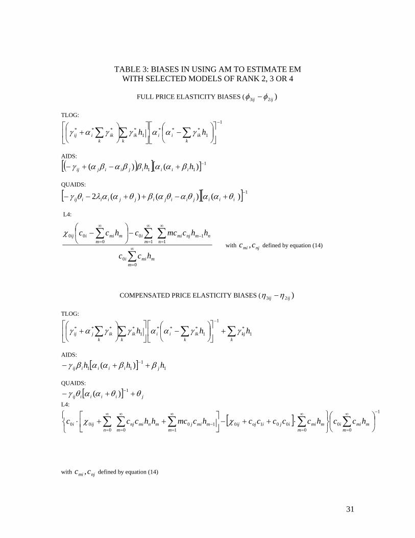
TABLE 1: BIASES IN USING EM TO ESTIMATE ME WITH SELECTED MODELS OF RANK 2, 3 OR 4
FULL PRICE ELASTICITY BIASES ( )12 ijij φφ −
TLOG:
1
1***
1**
−
⎥⎦
⎤⎢⎣
⎡⎟⎠
⎞⎜⎝
⎛−⎥
⎦
⎤⎢⎣
⎡− ∑∑
kikii
kikij hh γααγγ
AIDS:
( )[ ][ ] 111 )() −+− hh iiiiijij βααββαγ
QUAIDS:
( )( )[ ][ ] 121 )(2))(( −+−+−−+− iiiijiiijijiiijij hh θαααβλλβαγθαβαγ
L4:
∑
∑∑∞
=
∞
=
∞
=
⎟⎠
⎞⎜⎝
⎛−
00
000
0
mmmii
im
mmijm
mmiij
hcc
chhc χχ with mic defined by equation (14)
COMPENSATED PRICE ELASTICITY BIASES ( )12 ijij ηη −
TLOG:
1
1***
2**
1*****
1******
)2(
−
⎥⎦
⎤⎢⎣
⎡⎟⎠
⎞⎜⎝
⎛−
⎪⎪
⎭
⎪⎪
⎬
⎫
⎪⎪
⎩
⎪⎪
⎨
⎧
⎥⎦
⎤⎢⎣
⎡⎟⎠
⎞⎜⎝
⎛++−+
⎥⎦
⎤⎢⎣
⎡⎥⎦
⎤⎢⎣
⎡−−−
∑∑ ∑∑∑∑
∑∑ ∑
kikii
k kkj
kik
kkj
kikkjii
kik
k kikjkjiij
hhh
hγαα
γγγγγαα
γγαγαγ
AIDS:
( )[ ][ ] 11211 )()()( −++++−+ hhhh iiiijijijiijijiij βαααβββββαβαβααγ
QUAIDS:
[ ] 1
432
1 )())2()((
)()( −+⎥⎥⎦
⎤
⎢⎢⎣
⎡
++++++++−
++−+iii
jiijjiijjiijijijiji
jijiijiijiij
hhh
hθαα
λλλλλβλβλαλββλββλαα
βββαβααθααγ
L4:
( )( )1
000
0001
1001000
−∞
=
∞
=+
∞
=
∞
=−+
∞
=
∞
=
∞
=
⎟⎠
⎞⎜⎝
⎛
⎭⎬⎫
⎩⎨⎧
⎟⎠
⎞⎜⎝
⎛++−++ ∑∑∑∑∑∑∑
mmmiii
nnmnjmi
mnnmnjmi
mmmmij
mmmiiojijij hccchcchcmchhccccc χχ
with njmi cc , defined by equation (14)
28
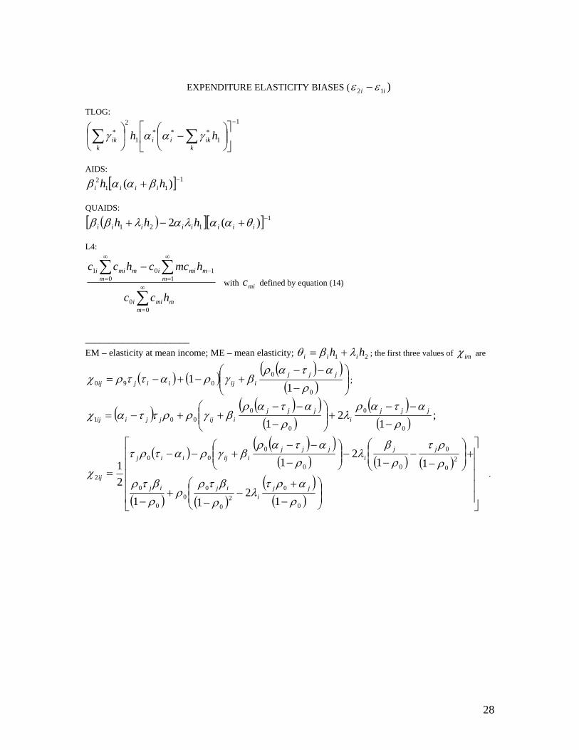
EXPENDITURE ELASTICITY BIASES ( )12 ii εε −
TLOG:
1
1***
1
2*
−
⎥⎦
⎤⎢⎣
⎡⎟⎠
⎞⎜⎝
⎛−⎟
⎠
⎞⎜⎝
⎛ ∑∑k
ikiik
ik hh γααγ
AIDS:
[ ] 111
2 )( −+ hh iiii βααβ QUAIDS:
( )[ ][ ] 1121 )(2 −+−+ iiiiiiii hhh θααλαλββ
L4:
∑
∑ ∑∞
=
∞
=
∞
=−−
00
0 1101
mmmii
m mmmiimmii
hcc
hmcchcc with mic defined by equation (14)
______________________ EM – elasticity at mean income; ME – mean elasticity; 21 hh iii λβθ += ; the first three values of imχ are
( ) ( ) ( )( )( ) ⎟⎟
⎠
⎞⎜⎜⎝
⎛−
−−+−+−=
0
0090 1
1ρ
αταρβγραττρχ jjj
iijiijij ;
( ) ( )( )( )
( )( ) ;1
21 0
0
0
0001 ρ
αταρλ
ραταρ
βγρρτταχ−
−−+⎟⎟
⎠
⎞⎜⎜⎝
⎛−
−−++−= jjj
ijjj
iijjjiij
( ) ( )( )( ) ( ) ( )
( ) ( )( )( ) ⎥
⎥⎥⎥⎥
⎦
⎤
⎢⎢⎢⎢⎢
⎣
⎡
⎟⎟⎠
⎞⎜⎜⎝
⎛
−
+−
−+
−
+⎟⎟⎠
⎞⎜⎜⎝
⎛
−−
−−⎟⎟
⎠
⎞⎜⎜⎝
⎛−
−−+−−
=
0
02
0
00
0
0
20
0
00
000
2
12
11
112
1
21
ραρτ
λρ
βτρρ
ρβτρ
ρ
ρτρ
βλ
ραταρ
βγρατρτ
χjj
iijij
jji
jjjiijiij
ij .
29
TABLE 2: BIASES IN USING AM TO ESTIMATE ME
FULL PRICE ELASTICITY BIASES ( )13 ijij φφ −
TLOG: 1
1**
1**
−
⎥⎦
⎤⎢⎣
⎡+−⎥
⎦
⎤⎢⎣
⎡− ∑∑∑
kiki
kik
kkj hh γαγγ
AIDS:
[ ][ ] 111
−+− hh iiji βαββ
QUAIDS:
L4:
∑
∑ ∑∑∞
=
∞
=
∞
=−
∞
=
−−
0
1 11
1
mmmi
mn
nmnjmi
mmmij
hc
hhcmchκ with njmi cc , defined by equation (14)
COMPENSATED PRICE ELASTICITY BIASES ( )13 ijij ηη −
TLOG:
( )1
1**
212
1**
−
⎥⎦
⎤⎢⎣
⎡+−⎥
⎦
⎤⎢⎣
⎡−− ∑∑ ∑
kiki
k kkjik hhhh γαγγ
AIDS:
[ ][ ] 1121
21
−+−− hhhh iiji βαββ
QUAIDS:
[ ][ ] 134
22232112
21 )2())(()( −+−−+−−++−− iijijijiji hhhhhhhhhh θαλλβλλβββ
L4:
[ ]
∑
∑∑∑∑∑∞
=
−+
∞
=
∞
=
∞
=+
∞
=
∞
=
−−−
0
111111
mmmi
nmn
njmimm
mmijnmnmn
njmim
hc
hcmchhhhcc κ
with njmi cc , defined by equation (14)
[ ][ ] 112 )2( −++− iijiiji hh θαθλββλ
30
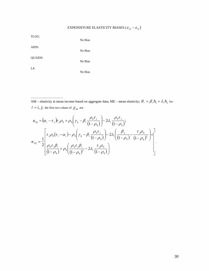
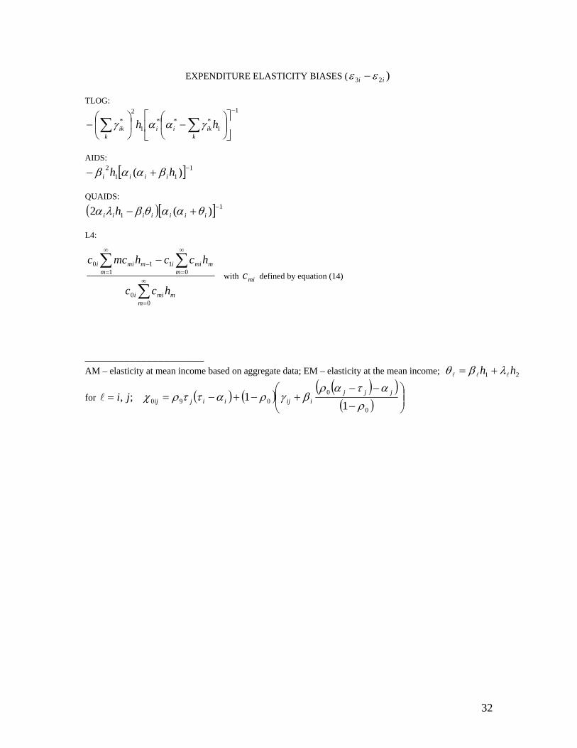
EXPENDITURE ELASTICITY BIASES ( )13 ii εε −
TLOG: No Bias AIDS: No Bias QUAIDS: No Bias L4: No Bias _____________________ AM – elasticity at mean income based on aggregate data; ME – mean elasticity; 21 hh lll λβθ += for
;, ji=l the first two values of imχ are
( ) ( ) ( ) ;12
1 0
0
0
0001 ρ
τρλ
ρτρ
βγρρττακ−
−⎟⎟⎠
⎞⎜⎜⎝
⎛−
−+−= ji
jiijjjiij
( ) ( ) ( ) ( )
( ) ( ) ( ) ⎥⎥⎥⎥⎥
⎦
⎤
⎢⎢⎢⎢⎢
⎣
⎡
⎟⎟⎠
⎞⎜⎜⎝
⎛
−−
−+
−
+⎟⎟⎠
⎞⎜⎜⎝
⎛
−−
−−⎟⎟
⎠
⎞⎜⎜⎝
⎛−
−−−
=
0
02
0
00
0
0
20
0
00
000
2
12
11
112
1
21
ρρτ
λρ
βτρρ
ρβτρ
ρ
ρτρ
βλ
ρτρ
βγρατρτ
κj
iijij
jji
jiijiij
ij .
31
TABLE 3: BIASES IN USING AM TO ESTIMATE EM WITH SELECTED MODELS OF RANK 2, 3 OR 4
FULL PRICE ELASTICITY BIASES ( )23 ijij φφ −
TLOG:
1
1***
1****
−
⎥⎦
⎤⎢⎣
⎡⎟⎠
⎞⎜⎝
⎛−⎥
⎦
⎤⎢⎣
⎡⎟⎠
⎞⎜⎝
⎛+ ∑∑∑
kikii
kik
kikiij hh γααγγαγ
AIDS:
( )[ ][ ] 111 )()( −+−+− hh iiiijiijij βααββαβαγ
QUAIDS:
[ ][ ] 1)()()(2 −+−++−− iiijiijijjiiiij θααθαθαβθααλθγ
L4:
∑
∑∑∑∞
=
∞
=−
∞
=
∞
=
−⎟⎠
⎞⎜⎝
⎛−
00
11
10
000
mmmii
nn
mnjmim
im
mmiiij
hcc
hhcmcchccχ with njmi cc , defined by equation (14)
COMPENSATED PRICE ELASTICITY BIASES ( )23 ijij ηη −
TLOG:
∑∑∑∑ +⎥⎦
⎤⎢⎣
⎡⎟⎠
⎞⎜⎝
⎛−⎥
⎦
⎤⎢⎣
⎡⎟⎠
⎞⎜⎝
⎛+
−
kkj
kikii
kik
kikjij hhh 1
*1
1***
1**** γγααγγαγ
AIDS:
[ ] 11
11 )( hhh jiiiiij ββααβγ ++− −
QUAIDS:
[ ] jiiiiij θθααθγ ++− −1)(
L4:
[ ]1
00
00010
0 110
000
−∞
=
∞
=
∞
=
∞
=−
∞
=
⎟⎠
⎞⎜⎝
⎛
⎭⎬⎫
⎩⎨⎧
⋅++−⎥⎦
⎤⎢⎣
⎡++⋅ ∑∑∑ ∑∑
mmmii
mmmiijiojij
m mmmijmnminj
niji hcchccccchcmchhccc χχ
with njmi cc , defined by equation (14)
32
EXPENDITURE ELASTICITY BIASES ( )23 ii εε −
TLOG: 1
1***
1
2*
−
⎥⎦
⎤⎢⎣
⎡⎟⎠
⎞⎜⎝
⎛−⎟
⎠
⎞⎜⎝
⎛− ∑∑
kikii
kik hh γααγ
AIDS:
[ ] 111
2 )( −+− hh iiii βααβ QUAIDS:
( )[ ] 11 )(2 −+− iiiiiii h θααθβλα
L4:
∑
∑∑∞
=
∞
=
∞
=− −
00
01
110
mmmii
mmmii
mmmii
hcc
hcchmcc with mic defined by equation (14)
_____________________ AM – elasticity at mean income based on aggregate data; EM – elasticity at the mean income; 21 hh lll λβθ +=
for ;, ji=l ( ) ( ) ( )( )( ) ⎟⎟
⎠
⎞⎜⎜⎝
⎛−
−−+−+−=
0
0090 1
1ρ
αταρβγραττρχ jjj
iijiijij
33
TABLE 4: ELASTICITY BIASES FOR TLOG DEMAND SYSTEM
Food Alcohol Fuel Clothing Transport Services Sweden Germany Sweden Germany Sweden Germany Sweden Germany Sweden Germany Sweden Germany Full Own-Price ME -0.535 -0.521 -1.627 -1.551 -0.507 -0.498 -0.618 -0.615 -0.702 -0.708 -0.736 -0.745 EM -0.564 -0.564 -1.740 -1.740 -0.517 -0.517 -0.622 -0.622 -0.696 -0.696 -0.724 -0.724 AM -0.542 -0.507 -1.639 -1.571 -0.508 -0.499 -0.618 -0.615 -0.703 -0.709 -0.738 -0.750 EM – ME -0.029 -0.043 -0.113 -0.189 -0.010 -0.019 -0.004 -0.007 0.006 0.012 0.012 0.021 AM - ME -0.007 -0.014 -0.012 -0.020 -0.001 -0.001 -0.000 -0.000 -0.001 -0.001 -0.002 -0.005 Compensated Own-Price ME -0.325 -0.301 -1.432 -1.334 -0.441 -0.433 -0.527 -0.524 -0.480 -0.481 -0.550 -0.549 EM -0.350 -0.350 -1.580 -1.580 -0.450 -0.450 -0.530 -0.530 -0.480 -0.480 -0.550 -0.550 AM -0.345 -0.338 -1.468 -1.391 -0.442 -0.435 -0.527 -0.525 -0.483 -0.485 -0.558 -0.563 EM – ME -0.025 -0.049 -0.148 -0.246 -0.009 -0.017 -0.003 -0.006 0.000 0.001 -0.000 -0.001 AM - ME -0.020 -0.037 -0.036 -0.057 -0.001 -0.002 -0.000 -0.001 -0.003 -0.004 -0.008 -0.014 Expenditure ME 0.590 0.572 2.113 1.996 0.837 0.834 0.919 0.919 1.195 1.191 1.426 1.408 EM 0.610 0.610 2.290 2.290 0.840 0.840 0.920 0.920 1.200 1.200 1.450 1.450 AM 0.590 0.572 2.113 1.996 0.837 0.834 0.919 0.919 1.195 1.191 1.426 1.408 EM – ME 0.020 0.038 0.177 0.294 0.003 0.006 0.001 0.001 0.005 0.009 0.024 0.042 AM - ME 0.000 0.000 0.000 0.000 0.000 0.000 0.000 0.000 0.000 0.000 0.000 0.000
34
TABLE 5: ELASTICITY BIASES FOR AIDS DEMAND SYSTEM
Food Alcohol Fuel Clothing Transport Services Sweden Germany Sweden Germany Sweden Germany Sweden Germany Sweden Germany Sweden Germany Full Own-Price ME -0.542 -0.521 -1.639 -1.571 -0.508 -0.499 -0.618 -0.615 -0.703 -0.709 -0.738 -0.750 EM -0.564 -0.564 -1.740 -1.740 -0.517 -0.517 -0.622 -0.622 -0.696 -0.696 -0.724 -0.724 AM -0.548 -0.534 -1.651 -1.592 -0.508 -0.499 -0.618 -0.615 -0.704 -0.711 -0.741 -0.755 EM – ME -0.022 -0.043 -0.101 -0.169 -0.009 -0.018 -0.004 -0.007 -0.007 0.013 0.014 0.026 AM - ME -0.006 -0.013 -0.012 -0.021 -0.000 -0.000 -0.000 -0.000 -0.001 -0.002 -0.003 -0.005 Compensated Own-Price ME -0.332 -0.315 -1.445 -1.354 -0.441 -0.434 -0.527 -0.525 -0.481 -0.482 -0.553 -0.555 EM -0.350 -0.350 -1.580 -1.580 -0.450 -0.450 -0.530 -0.530 -0.480 -0.480 -0.550 -0.550 AM -0.352 -0.352 -1.480 -1.411 -0.442 -0.435 -0.527 -0.525 -0.484 -0.487 -0.561 -0.568 EM – ME -0.018 -0.035 -0.135 -0.226 -0.009 -0.016 -0.003 -0.005 0.001 0.002 0.003 0.005 AM - ME -0.020 -0.037 -0.035 -0.057 -0.001 -0.001 -0.000 -0.000 -0.003 -0.005 -0.008 -0.013 Expenditure ME 0.590 0.572 2.113 1.996 0.837 0.834 0.919 0.919 1.195 1.191 1.426 1.408 EM 0.610 0.610 2.290 2.290 0.840 0.840 0.920 0.920 1.200 1.200 1.450 1.450 AM 0.590 0.590 2.113 2.113 0.837 0.834 0.919 0.919 1.195 1.191 1.426 1.408 EM – ME 0.020 0.038 0.177 0.294 0.003 0.006 0.001 0.001 0.005 0.009 0.024 0.042 AM - ME 0.000 0.000 0.000 0.000 0.000 0.000 0.000 0.000 0.000 0.000 0.000 0.000
35
TABLE 6: ELASTICITY BIASES FOR QUAIDS DEMAND SYSTEM
Food Alcohol Fuel Clothing Transport Services Sweden Germany Sweden Germany Sweden Germany Sweden Germany Sweden Germany Sweden Germany Full Own-Price ME -0.538 -0.513 -1.642 -1.576 -0.565 -0.601 -0.586 -0.549 -0.713 -0.727 -0.715 -0.706 EM -0.564 -0.564 -1.740 -1.740 -0.517 -0.517 -0.622 -0.622 -0.696 -0.696 -0.724 -0.724 AM -0.545 -0.527 -1.654 -1.596 -0.566 -0.604 -0.587 -0.551 -0.714 -0.729 -0.718 -0.712 EM – ME -0.026 -0.051 -0.098 -0.164 0.048 0.084 -0.036 -0.073 0.017 0.031 -0.009 -0.018 AM - ME -0.007 -0.014 -0.012 -0.020 -0.001 -0.003 -0.001 -0.002 -0.001 -0.002 -0.003 -0.006 Compensated Own-Price ME -0.331 -0.311 -1.449 -1.361 -0.483 -0.503 -0.506 -0.479 -0.483 -0.484 -0.547 -0.543 EM -0.350 -0.350 -1.580 -1.580 -0.450 -0.450 -0.530 -0.530 -0.480 -0.480 -0.550 -0.550 AM -0.352 -0.352 -1.484 -1.417 -0.482 -0.506 -0.508 -0.485 -0.487 -0.491 -0.550 -0.550 EM – ME -0.019 -0.039 -0.131 -0.219 0.033 0.053 -0.024 -0.051 0.003 0.004 -0.003 -0.007 AM - ME -0.021 -0.041 -0.035 -0.056 0.001 -0.003 -0.002 -0.006 -0.004 -0.007 -0.003 -0.007 Expenditure ME 0.582 0.555 2.114 1.996 0.958 1.044 0.845 0.769 1.211 1.220 1.394 1.347 EM 0.610 0.610 2.290 2.290 0.840 0.840 0.920 0.920 1.200 1.200 1.450 1.450 AM 0.582 0.555 2.114 1.996 0.958 1.044 0.845 0.769 1.211 1.220 1.394 1.347 EM – ME 0.028 0.055 0.176 0.294 -0.118 -0.204 0.075 0.151 -0.011 -0.020 0.056 0.103 AM - ME 0.000 0.000 0.000 0.000 0.000 0.000 0.000 0.000 0.000 0.000 0.000 0.000
36
TABLE 7: ELASTICITY BIASES FOR L4 DEMAND SYSTEM
Food Alcohol Fuel Clothing Transport Services Sweden Germany Sweden Germany Sweden Germany Sweden Germany Sweden Germany Sweden Germany Full Own-Price ME -0.532 -0.496 -1.612 -1.534 -0.558 -0.588 -0.578 -0.536 -0.717 -0.733 -0.714 -0.711 EM -0.564 -0.564 -1.740 -1.740 -0.517 -0.517 -0.622 -0.622 -0.696 -0.696 -0.724 -0.724 AM -0.536 -0.505 -1.629 -1.563 -0.557 -0.588 -0.578 -0.537 -0.719 -0.738 -0.718 -0.718 EM – ME -0.032 -0.068 -0.128 -0.206 0.041 0.071 -0.044 -0.086 0.021 0.037 -0.010 -0.013 AM - ME -0.004 -0.009 -0.017 -0.029 0.001 0.000 -0.000 -0.001 -0.002 -0.005 -0.004 -0.007 Compensated Own-Price ME -0.332 -0.306 -1.406 -1.296 -0.478 -0.494 -0.501 -0.469 -0.480 -0.478 -0.543 -0.542 EM -0.350 -0.350 -1.580 -1.580 -0.450 -0.450 -0.530 -0.530 -0.480 -0.480 -0.550 -0.550 AM -0.356 -0.354 -1.451 -1.370 -0.476 -0.495 -0.503 -0.476 -0.487 -0.491 -0.548 -0.552 EM – ME -0.018 -0.044 -0.174 -0.284 0.028 0.044 -0.029 -0.061 0.000 -0.002 -0.007 -0.008 AM - ME -0.024 -0.048 -0.045 -0.074 0.002 -0.001 -0.002 -0.007 -0.007 -0.013 -0.005 -0.010 Expenditure ME 0.555 0.499 2.110 1.996 0.944 1.023 0.827 0.732 1.221 1.238 1.400 1.358 EM 0.610 0.610 2.290 2.290 0.840 0.840 0.920 0.920 1.200 1.200 1.450 1.450 AM 0.555 0.499 2.110 1.996 0.958 1.023 0.827 0.732 1.221 1.258 1.400 1.358 EM – ME 0.055 0.111 0.180 0.294 -0.104 -0.183 0.093 0.188 -0.021 -0.038 0.050 0.092 AM - ME 0.000 0.000 0.000 0.000 0.000 0.000 0.000 0.000 0.000 0.000 0.000 0.000
Appendix A – Theorem and Corollary Proofs
Proof of Theorem 1: (i) Using equations (3) and (4) (and using the normalization restrictions, both here and subsequently), the mean full price elasticity ( ij1φ ) is given by
( )
( )
)1(ln
lnln
lnln
ln
lnln
0
0
1
0
1
0
1
11
Ahc
hp
c
Xx
W
xp
c
w
xp
c
wp
w
pq
mmmi
mm j
mi
ij
K
k
k
i
mk
m j
mi
ij
K
k i
ik
ik
mk
m j
mi
ij
K
k i
ik
ik
j
ik
ij
i
ikK
k j
ikij
∑
∑
∑∑
∑∑
∑
∑
∞
=
∞
=
=
∞
=
=
∞
=
=
=
⎥⎥⎦
⎤
⎢⎢⎣
⎡
∂∂
+−=
⎟⎟⎟⎟⎟⎟
⎠
⎞
⎜⎜⎜⎜⎜⎜
⎝
⎛
⎟⎟⎟⎟⎟⎟
⎠
⎞
⎜⎜⎜⎜⎜⎜
⎝
⎛
⎥⎥⎦
⎤
⎢⎢⎣
⎡
∂∂
+−=
⎟⎟⎟⎟⎟⎟
⎠
⎞
⎜⎜⎜⎜⎜⎜
⎝
⎛
⎥⎥⎦
⎤
⎢⎢⎣
⎡
∂∂
+−=
⎟⎟⎟⎟⎟
⎠
⎞
⎜⎜⎜⎜⎜
⎝
⎛∂∂
+−=
∂∂
=
δ
δ
δ
δ
φ
38
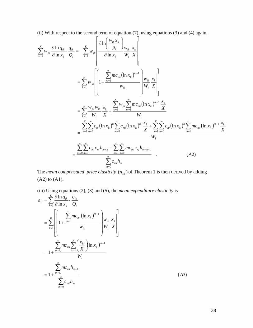
(ii) With respect to the second term of equation (7), using equations (3) and (4) again,
( )
( )
( ) ( ) ( ) ( )
)2(.
lnlnlnln
ln
ln1
ln
ln
lnln
0
1 01
0 0
1 0 1
1
1 0 0
1
1
1
1
1
1
1
11
Ahc
hcmchcc
WXx
xmcxcXx
xcxc
WXx
xmcw
Xx
Www
Xx
Ww
w
xmcw
Xx
Ww
xp
xw
wQq
xq
w
mmmi
m nnmnjmi
m nnmnjmi
i
kK
k n m
mkmi
nknj
kK
k n m
mkmi
nknj
i
k
m
mkmi
K
kjk
kK
k i
ikjk
K
k
k
i
ik
ik
m
mkmi
jk
K
k
k
i
ik
k
i
kik
jki
ikK
k k
ikjk
∑
∑∑∑∑
∑∑ ∑∑∑ ∑
∑∑∑
∑∑
∑∑
∞
=
∞
=
∞
=−+
∞
=
∞
=+
=
∞
=
∞
=
−
=
∞
=
∞
=
∞
=
−
=
=
=
∞
=
−
==
+=
+=
+=
⎥⎥⎥⎥
⎦
⎤
⎢⎢⎢⎢
⎣
⎡
⎟⎟⎟⎟
⎠
⎞
⎜⎜⎜⎜
⎝
⎛
+=
⎥⎥⎥⎥⎥
⎦
⎤
⎢⎢⎢⎢⎢
⎣
⎡
∂
⎟⎟⎠
⎞⎜⎜⎝
⎛∂
=⋅∂∂
The mean compensated price elasticity )( 1ijη of Theorem 1 is then derived by adding (A2) to (A1). (iii) Using equations (2), (3) and (5), the mean expenditure elasticity is
( )
( )
)3(1
ln1
ln1
lnln
0
1,1
1
1
,1
1
1
1
11
Ahc
hcm
W
xXx
cm
Xx
Ww
w
xmc
xq
mmmi
mmim
i
K
k
mk
kmi
m
K
k
k
i
ik
ik
m
mkmi
i
ikK
k k
iki
∑
∑
∑∑
∑∑
∑
∞
=
−
∞
=
=
−∞
=
=
∞
=
−
=
+=
⎟⎠⎞
⎜⎝⎛
+=
⎥⎥⎥⎥
⎦
⎤
⎢⎢⎢⎢
⎣
⎡
⎟⎟⎟⎟
⎠
⎞
⎜⎜⎜⎜
⎝
⎛
+=
⋅∂∂
=ε
39
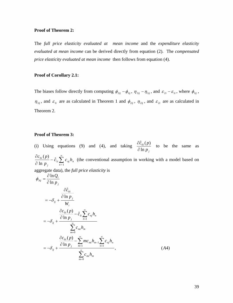
Proof of Theorem 2:
The full price elasticity evaluated at mean income and the expenditure elasticity
evaluated at mean income can be derived directly from equation (2). The compensated
price elasticity evaluated at mean income then follows from equation (4).
Proof of Corollary 2.1:
The biases follow directly from computing ijij 12 φφ − , ijij 12 ηη − , and ii 12 εε − , where ij1φ ,
ij1η , and i1ε are as calculated in Theorem 1 and ij2φ , ij2η , and i2ε are as calculated in
Theorem 2.
Proof of Theorem 3:
(i) Using equations (9) and (4), and taking j
i
ppc
ln)(ˆ0
∂∂
to be the same as
∑∞
=
−∂
∂
11
0 ˆln
)(
nnnji
j
i hccppc
(the conventional assumption in working with a model based on
aggregate data), the full price elasticity is
)4(,ln
)(
ˆln
)(
lnˆ
lnln
0
111
0
0
11
0
0
3
Ahc
hchmcppc
hc
hccppc
Wp
cpQ
mmmi
nnnj
mmmi
j
i
ij
mmmi
nnnji
j
i
ij
i
j
i
ij
j
iij
∑
∑∑
∑
∑
∞
=
∞
=
∞
=−
∞
=
∞
=
−∂∂
+−=
−∂∂
+−=
∂∂
+−=
∂∂
=
δ
δ
δ
φ
40
(ii) The second component of equation (7), again using equations (6) and (3), can be written as
)5(
lnln
0
0 11
00
11
Ahc
hhcmchhcc
hmcWWW
XQ
W
mmmi
m mmnminj
nmnminj
n
mmmii
i
jij
∑
∑ ∑∑∑
∑
∞
=
∞
=
∞
=−
∞
=
∞
=
∞
=−
+=
⎟⎠
⎞⎜⎝
⎛+=
∂∂
The compensated price elasticity ( ij3η ) is then obtained by adding (A5) to (A4).
(iii) The expenditure elasticity evaluated at its mean, in Theorem 3 is
).6(1
lnln
0
11
3
Ahc
hmc
XQ
mmmi
mm
mi
ii
∑
∑∞
=
−
∞
=+=
∂∂
=ε
Proof of Corollary 3.1:
The biases follow directly from computing ijij 13 φφ − , ijij 13 ηη − , and ii 13 εε − , where ij1φ ,
ij1η , and i1ε are as calculated in Theorem 1 and ij3φ , ij3η , and i3ε are as calculated in
Theorem 3.
Proof of Corollary 3.2:
The biases follow directly from computing ijij 23 φφ − , ijij 23 ηη − , and ii 23 εε − , where ij2φ ,
ij2η , and i2ε are as calculated in Theorem 2 and ij3φ , ij3η , and i3ε are as calculated in
Theorem 3.
41
APPENDIX B: PARAMETER VALUES USED IN CALIBRATION
TABLE B1: UNDERLYING EM ELASTICITIES AND PARAMETERS OF MICRO MODEL
FOOD ALCOHOL FUEL CLOTHING TRANSPORT SERVICES EM
iiφ -0.564 -1.740 -0.517 -0.622 -0.696 -0.724
iiη -0.350 -1.580 -0.450 -0.530 -0.480 -0.550
iε 0.610 2.290 0.840 0.920 1.200 1.450 TLOG
*iα -0.35 -0.07 -0.08 -0.10 -0.18 -0.12 *ijγ -0.2005 0.0581 -0.0396 -0.0386 -0.0482 -0.0266
∑j
ij*γ -0.1365 0.0903 -0.0128 -0.008 0.036 0.054
AIDS
iα 0.35 0.07 0.08 0.10 0.18 0.12
iiγ 0.105 -0.0455 0.0376 0.037 0.0612 0.0396
iβ -0.1365 0.0903 -0.0128 -0.008 0.036 0.054 QUAIDS
iα 0.35 0.07 0.08 0.10 0.18 0.12
iiγ 0.105 -0.0455 0.0376 0.037 0.0612 0.0396
iβ -0.1365 0.0903 -0.0128 -0.008 0.036 0.054
iλ -0.008 -0.002 0.037 -0.026 0.015 -0.027 L4
2.0 =ρ
iα 0.3325 0.0825 0.0475 0.105 0.185 0.1325
iiγ 0.1297 -0.0577 0.0417 0.0461 0.0764 0.0487
iβ -0.119 0.0778 0.0197 -0.013 0.031 0.0415
iλ -0.008 -0.002 0.037 -0.026 0.015 -0.027
iτ 0.42 0.02 0.21 0.08 0.16 0.07
42
TABLE B2: INCOME DISTRIBUTION PARAMETERS FOR SEVEN COUNTRIES
1h 2h 3h 4h Sweden .123 .242 .015 .113 Norway .142 .259 -.023 .168 Israel .166 .313 .006 .219 Canada .171 .321 -.007 .263 United Kingdom .172 .321 -.002 .232 United States .204 .367 -.016 .345 Germany .229 .456 .105 .412 NOTE: Calculations are based on after-tax family income quintile shares provided in table 2 of O’Higgins, Schmaus, and Stephenson (1989). See Denton and Mountain (2004) for details of the calculations.
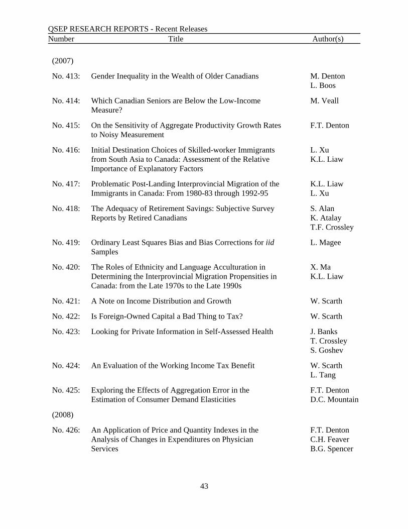
QSEP RESEARCH REPORTS - Recent ReleasesNumber Title Author(s)
43
(2007)
No. 413: Gender Inequality in the Wealth of Older Canadians M. DentonL. Boos
No. 414: Which Canadian Seniors are Below the Low-IncomeMeasure?
M. Veall
No. 415: On the Sensitivity of Aggregate Productivity Growth Ratesto Noisy Measurement
F.T. Denton
No. 416: Initial Destination Choices of Skilled-worker Immigrantsfrom South Asia to Canada: Assessment of the RelativeImportance of Explanatory Factors
L. XuK.L. Liaw
No. 417: Problematic Post-Landing Interprovincial Migration of theImmigrants in Canada: From 1980-83 through 1992-95
K.L. LiawL. Xu
No. 418: The Adequacy of Retirement Savings: Subjective SurveyReports by Retired Canadians
S. AlanK. AtalayT.F. Crossley
No. 419: Ordinary Least Squares Bias and Bias Corrections for iidSamples
L. Magee
No. 420: The Roles of Ethnicity and Language Acculturation inDetermining the Interprovincial Migration Propensities inCanada: from the Late 1970s to the Late 1990s
X. MaK.L. Liaw
No. 421: A Note on Income Distribution and Growth W. Scarth
No. 422: Is Foreign-Owned Capital a Bad Thing to Tax? W. Scarth
No. 423: Looking for Private Information in Self-Assessed Health J. BanksT. CrossleyS. Goshev
No. 424: An Evaluation of the Working Income Tax Benefit W. ScarthL. Tang
No. 425: Exploring the Effects of Aggregation Error in theEstimation of Consumer Demand Elasticities
F.T. DentonD.C. Mountain
(2008)
No. 426: An Application of Price and Quantity Indexes in theAnalysis of Changes in Expenditures on PhysicianServices
F.T. DentonC.H. FeaverB.G. Spencer

QSEP RESEARCH REPORTS - Recent ReleasesNumber Title Author(s)
44
No. 427: What Is Retirement? A Review and Assessment ofAlternative Concepts and Measures
F.T. DentonB.G. Spencer
No. 428: Pension Benefit Insurance and Pension Plan PortfolioChoice
T. CrossleyM. Jametti
(2009)
No. 429: Visiting and Office Home Care Workers’ OccupationalHealth: An Analysis of Workplace Flexibility and WorkerInsecurity Measures Associated with Emotional andPhysical Health
I.U. ZeytinogluM. DentonS. DaviesM.B. SeatonJ. Millen
No. 430: Where Would You Turn For Help? Older Adults’Knowledge and Awareness of Community SupportServices
M. DentonJ. PloegJ. TindaleB. HutchisonK. BrazilN. Akhtar-DaneshM. Quinlan
No. 431: New Evidence on Taxes and Portfolio Choice S. AlanK. AtalayT.F. CrossleyS.H. Jeon
No. 432: Cohort Working Life Tables for Older Canadians F.T. DentonC.H. FeaverB.G. Spencer
No. 433: Population Aging, Older Workers, and Canada’s LabourForce
F.T. DentonB.G. Spencer
No. 434: Patterns of Retirement as Reflected in Income TaxRecords for Older Workers
F.T. DentonR. FinnieB.G. Spencer
No. 435: Chronic Health Conditions: Changing Prevalence in anAging Population and Some Implications for the Deliveryof Health Care Services
F.T. DentonB.G. Spencer
No. 436: Income Replacement in Retirement: LongitudinalEvidence from Income Tax Records
F.T. DentonR. FinnieB.G. Spencer
QSEP RESEARCH REPORTS - Recent ReleasesNumber Title Author(s)
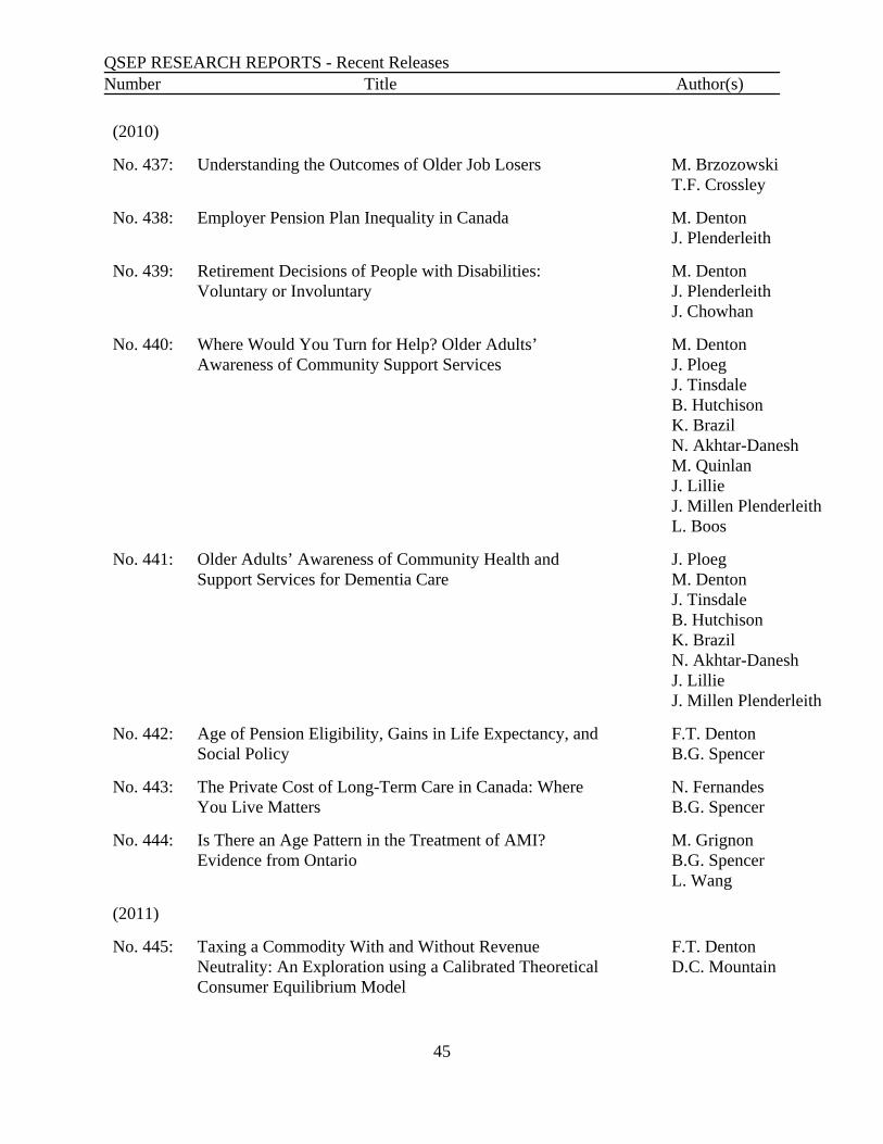
45
(2010)
No. 437: Understanding the Outcomes of Older Job Losers M. BrzozowskiT.F. Crossley
No. 438: Employer Pension Plan Inequality in Canada M. DentonJ. Plenderleith
No. 439: Retirement Decisions of People with Disabilities:Voluntary or Involuntary
M. DentonJ. PlenderleithJ. Chowhan
No. 440: Where Would You Turn for Help? Older Adults’Awareness of Community Support Services
M. DentonJ. PloegJ. TinsdaleB. HutchisonK. BrazilN. Akhtar-DaneshM. QuinlanJ. LillieJ. Millen PlenderleithL. Boos
No. 441: Older Adults’ Awareness of Community Health andSupport Services for Dementia Care
J. PloegM. DentonJ. TinsdaleB. HutchisonK. BrazilN. Akhtar-DaneshJ. LillieJ. Millen Plenderleith
No. 442: Age of Pension Eligibility, Gains in Life Expectancy, andSocial Policy
F.T. DentonB.G. Spencer
No. 443: The Private Cost of Long-Term Care in Canada: WhereYou Live Matters
N. FernandesB.G. Spencer
No. 444: Is There an Age Pattern in the Treatment of AMI?Evidence from Ontario
M. GrignonB.G. SpencerL. Wang
(2011)
No. 445: Taxing a Commodity With and Without RevenueNeutrality: An Exploration using a Calibrated TheoreticalConsumer Equilibrium Model
F.T. DentonD.C. Mountain
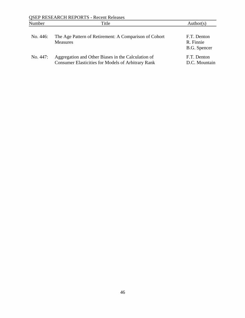
QSEP RESEARCH REPORTS - Recent ReleasesNumber Title Author(s)
46
No. 446: The Age Pattern of Retirement: A Comparison of CohortMeasures
F.T. DentonR. FinnieB.G. Spencer
No. 447: Aggregation and Other Biases in the Calculation ofConsumer Elasticities for Models of Arbitrary Rank
F.T. DentonD.C. Mountain