Robust Quantile Regression using a Generalized Class of Skewed

Distributions

Christian E. Galarzaa,b Victor H. Lachosb∗ Celso R. B. Cabralc

Luis M. Castrod

aDepartamento de Matematicas, Escuela Superior Politecnica del Litoral, ESPOL, EcuadorbDepartamento de Estatıstica, Universidade Estadual de Campinas, BrazilcDepartamento de Estatıstica, Universidade Federal do Amazonas, Brazil

dDepartamento de Estadıstica and CI2MA, Universidad de Concepcion, Chile

Abstract

It is well known that the widely popular mean regression model could be inadequate ifthe probability distribution of the observed responses do not follow a symmetric distribution.To deal with this situation, the quantile regression turns to be a more robust alternative foraccommodating outliers and the misspecification of the error distribution since it characterizesthe entire conditional distribution of the outcome variable. This paper presents a likelihood-based approach for the estimation of the regression quantiles based on a new family of skeweddistributions introduced by Wichitaksorn et al. (2014). This family includes the skewed versionof Normal, Student-t, Laplace, contaminated Normal and slash distribution, all with the zeroquantile property for the error term, and with a convenient and novel stochastic representationwhich facilitates the implementation of the EM algorithm for maximum-likelihood estimationof the pth quantile regression parameters. We evaluate the performance of the proposed EMalgorithm and the asymptotic properties of the maximum-likelihood estimates through empiricalexperiments and application to a real life dataset. The algorithm is implemented in the Rpackage lqr(), providing full estimation and inference for the parameters as well as simulationenvelopes plots useful for assessing the goodness-of-fit.

Keywords Quantile regression model; EM algorithm; Scale mixtures of Normal distributions.

1 Introduction

Quantile regression (QR) models have become increasingly popular since the seminal work ofKoenker & G Bassett (1978). In contrast to the mean regression model, QR belongs to a robustmodel family, which can give an overall assessment of the covariate effects at different quantilesof the outcome (Koenker, 2005). In particular, we can model the lower or higher quantiles of theoutcome to provide a natural assessment of covariate effects specific for those regression quantiles.Unlike conventional models, which only address the conditional mean or the central effects of thecovariates, QR models quantify the entire conditional distribution of the outcome variable. Inaddition, QR does not impose any distributional assumption on the error, except the requirementabout the zero conditional quantile. The foundations of the methods for independent data arenow consolidated, and some statistical methods for estimating and drawing inferences about con-ditional quantiles are provided by most of the available statistical programs (e.g., R, SAS, Matlaband Stata). For instance, just to name a few of them, in the well-known R package quantreg() is

∗Address for correspondence: Departamento de Estatıstica, Rua Sergio Buarque de Holanda, 651, Cidade Univer-sitaria Zeferino Vaz, Campinas, Sao Paulo, Brazil. CEP 13083-859. E-mail: hlachos@ime.unicamp.br

1

implemented as a variant of the Barrodale & Roberts (1977) simplex (BR) for linear programmingproblems described in Koenker & d’Orey (1987), where the standard errors are computed by therank inversion method (Koenker, 2005). Another method implemented in this popular package isthe Lasso Penalized Quantile Regression (LPQR), introduced by Tibshirani (1996), where a penaltyparameter is specified to determine how much shrinkage occurs in the estimation process. As itcan be seen, the QR model can be implemented in a wide range of different methodologies.

From a Bayesian point of view, Kottas & Gelfand (2001) considered the study of the medianregression, which is a special case of QR. In this context, these authors discussed a non-parametricapproach for the error distribution based on either Polya tree or Dirichlet process priors. Regardinggeneral quantile regression, Yu & Moyeed (2001) proposed a Bayesian modeling approach by usingthe asymmetric Laplace distribution (ALD), Kottas & Krnjajic (2009) developed Bayesian semi-parametric models for quantile regression using Dirichlet process mixtures for the error distribution.Kozumi & Kobayashi (2011) developed a simple and efficient Gibbs sampling algorithm for fittingthe quantile regression model based on a location-scale mixture representation of the ALD. Fromthe classical viewpoint, Benites et al. (2013), Zhou et al. (2014) and Tian et al. (2014) adjusteda linear QR model based on EM algorithm for maximum likelihood (ML) assuming ALD errors.Particularly Benites et al. (2013) showed that their approach out-performed other common non-parametric estimators as those obtained via BR and LPQR algorithms. While ALD has the zeroquantile property and a useful stochastic representation, it is not differentiable at zero, which couldlead to problems of numerical instability. Thus the Laplace density is a pretty strong assumptionin order to set a quantile regression model through the classical or Bayesian framework.

To overcome this deficiency, recently Wichitaksorn et al. (2014) introduced a generalized classof skew densities (SKD) for the analysis of QR that provides competing solutions to the ALD-basedformulation. The robust SKD class of distributions is constructed by mixing a skew-normal dis-tribution (SKN) proposed by Fernandez & Steel (1998) and the symmetric class of scale mixtureof normal (SMN) distributions proposed by Andrews & Mallows (1974). The SKN distributionis obtained by partitioning two scaled mixture of normal (Gaussian) distributions, which have askewness parameter defined in the interval (0, 1), allowing direct application to parametric quantileregression. On the other hand, employing scale mixture of normals facilitates efficient estimationvia Markov chain Monte Carlo (MCMC) methods and the EM algorithm. In fact, Wichitaksornet al. (2014) adopt a MCMC approach as a natural solution to estimation and inference by usingthe marginal representation of the SKD class of distributions. In contrast to the marginal approachadopted in Wichitaksorn et al. (2014), in this paper a novel stochastic representation is proposed,which allows the study of many of its properties and also the implementation of an efficient (andeasy) EM algorithm for ML estimation of the parameters at the pth level, with closed form ex-pressions at the E- and M- steps. Therefore, the main contribution of this paper is to proposea robust method for drawing inferences about conditional quantiles in linear regression problemsfrom a likelihood-based perspective. Moreover, the proposed EM-type algorithm has been codedand implemented in the R package lqr() (Galarza et al., 2015), which is available for downloadat CRAN repository. A great advantage of this package is that it offers an automatic fit of all theSKD distributions taking into consideration.

The rest of the paper proceeds as follows. Section 2 presents the construction of the SKD familyof distributions as a scale mixture of skew normal distribution and some important propositionsand properties of this family. Section 3 introduces the QR model and the EM algorithm for MLestimation as well as the standard errors. Section 4 presents simulation studies of finite sampleperformance and robustness of our proposed method. An application of the EM algorithm to adataset examining some characteristics of Australian athletes available from the Australian Instituteof Sport (AIS) is presented in Section 5. Finally, Section 6 closes the paper, sketching some futureresearch directions.

2

2 The SKD family of distributions

In order to define the SKD class of distributions, we first make some remarks related to the skew-normal (SKN) distributions as defined by Wichitaksorn et al. (2014). Thus, in the following wepresent some definitions where we explain first the fundamental concept of the SKN distributionand its relation with the SKD family of distributions.

2.1 Preliminaries

As defined in Wichitaksorn et al. (2014), we say that a random variable X has a skew-normal(SKN) distribution with location parameter µ, scale parameter σ > 0 and skewness parameterp ∈ (0, 1), if its probability density function (pdf) is given by

f(x|µ, σ, p) = 2

[p φ

(x

∣∣∣∣µ,σ2

4(1− p)2

)Ix ≤ µ+ (1− p)φ

(x

∣∣∣∣µ,σ2

4p2

)Ix > µ

], (1)

where φ(·|µ, σ2) represents the pdf of the normal distribution with mean µ and variance σ2 (N(µ, σ2))and I· denotes the indicator function. By convention, we shall write X ∼ SKN(µ, σ, p). Notethat, P (X ≤ µ) = p and P (x > µ) = 1− p, which allows a direct application to quantile regressionproblems. When p = 0.5 we have the symmetric N(µ, σ2) distribution. Also, the pdf in (1) is con-structed as a mixture of two truncated normal distributions with weights p and 1− p respectively.Therefore, it can be conveniently written as

f(x|µ, σ, p) = 4p(1 − p)√2πσ2

exp

−2ρ2p

(x− µ

σ

), (2)

where ρp(·) is the so called check (or loss) function defined by ρp(u) = u(p − Iu < 0). It isimportant to remark that the SKN distribution is closed under location-scale transformations, i.e.,if Z ∼ SKN(0, 1, p), then X = µ+σZ ∼ SKN(µ, σ, p). Moreover, the SKN distribution has a usefulstochastic representation, given in the next result. The proof can be found in the Appendix.

Lemma 1. Let T0 ∼ N(0, 1) and I with probability function

P

(I = − 1

2(1 − p)

)= p and P

(I =

1

2p

)= 1− p,

be independent. Then, the random variable with stochastic representation

X = µ+ σI|T0|,follows a SKN(µ, σ, p) distribution.

2.2 Scale mixture of normal distributions

The family of scale mixture of normal (SMN) distributions (Andrews & Mallows, 1974; Lange &Sinsheimer, 1993) is a wide class of thick-tailed distributions including the normal one as a specialcase. This class of symmetric distributions also includes the Student-t (T), slash (S), contaminatednormal (CN), among many others. The SMN class can be conveniently represented using thefollowing stochastic representation,

W = µ+ σκ(U)1/2T0,

where µ is a location parameter, κ(·) is the weight function, U is positive random variable withpdf h(u|ν) and cumulative distribution function (cdf) H(u|ν), ν is a scalar or vector parameterindexing the distribution of U and T0 ∼ N(0, 1), with U independent of T0. Under this setup, themarginal pdf of Y is given by

f(w|µ, σ,ν) =∫∞0 φ

(w|µ, κ(u)σ2

)dH(u|ν).

We shall use W ∼ SMN(µ, σ2,ν) to denote this class of distributions.

3

2.3 A family of zero-quantile skewed distributions

This new class of distributions, defined by Wichitaksorn et al. (2014), is constructed as a scalemixture of SKN distributions. We say that Y follows a skewed distribution (denoted by SKD)with location parameter µ, scale parameter σ and skewness parameter p, if Y can be representedstochastically as

Y = µ+ σκ(U)1/2Z, (3)

where Z ∼ SKN(0, 1, p). A direct consequence of this definition is that, as the SKN distribution,P (Y ≤ µ) = p and P (Y > µ) = 1− p.

From the stochastic representation (3), the conditional distribution of Y given U = u isSKN(µ, κ(u)1/2σ, p). Then, integrating out U , we have that the marginal pdf of Y is

f(y|µ, σ, p,ν) =∫ ∞

0

4p(1− p)√2πκ(u)σ2

exp

−2ρ2p

(y − µ

κ1/2(u)σ

)dH(u|ν), (4)

and consequently, several skewed and thick-tailed distributions can be obtained from different speci-fications of the weight function κ(·) and pdf h(u|ν). Alternatively, another stochastic representationfor the SKD distribution can be provided. This representation is given in the following result, whoseproof is given in Appendix.

Lemma 2. Let T0 ∼ N(0, 1) and U a positive random variable, with U independent of T0. Let I bethe discrete random variable defined in Lemma 1. Then, Y ∼ SKD(µ, σ, p,ν) can be stochasticallyrepresented as

Yd= µ+ σκ(U)1/2I|T0|.

Table 1 presents some particular cases belonging to the SKD family, namely, the skewed Student-t (SKT(µ, σ, p, ν)); skewed Laplace (SKL(µ, σ, p)); skewed slash (SKS(µ, σ, p, ν)) and skewed con-taminated normal (SKCN(µ, σ, p, ν, γ)), respectively. Moreover, Figure 1 presents the pdf associatedto these members considering µ = 0 and σ = 1. In particular, this figure shows how the skewnesschanges for different values of parameter p. It is important to remark that, when p = 0.5 thesedistributions turn to be symmetrical.

Distribution κ(u) h(u|ν) f(y|µ, σ,ν)

skewed Student-t u−1 G(ν2 ,ν2 )

4p(1−p)Γ( ν+12 )

Γ( ν2 )

√2πσ2

4ν ρ

2p

(y−µσ

)+ 1

− ν+12

skewed Laplace u Exp(2) 2p(1−p)σ exp

−2ρp

(y−µσ

)

skewed slash u−1 Beta(ν, 1) ν

∫ 1

0uν−1φskd(y|µ, u−1/2σ, p)du

skewed cont. normal u−1 νIu = γ+ (1− ν)Iu = 10 ≤ ν, γ ≤ 1,

νφskd(y|µ, γ−1/2σ, p) + (1− ν)φskd(y|µ, σ, p)

Table 1: κ(·), h(u|ν) and pdf for some members of the SKD family. G(α, β) denotes the Gammadistribution with shape parameter α > 0 and rate parameter β > 0, Exp(β) denotes the exponentialdistribution with mean β, Beta(α, β) denotes the Beta distribution and φskd(y|µ, σ, p) denotes thepdf of the SKN distribution defined in (2).

An interesting result related to the moments of the SKD distributions is presented next.

4

(a) Skew normal

−6 −4 −2 0 2 4 6

0.0

0.1

0.2

0.3

0.4

0.5

de

nsity

p = 0.1

p = 0.5

p = 0.7

(b) Skew Student-t

−6 −4 −2 0 2 4 6

0.0

0.1

0.2

0.3

0.4

0.5

de

nsity

p = 0.1

p = 0.5

p = 0.7

(c) Skew Laplace

−6 −4 −2 0 2 4 6

0.0

0.1

0.2

0.3

0.4

0.5

de

nsity

p = 0.1

p = 0.5

p = 0.7

(d) Skew slash

−6 −4 −2 0 2 4 6

0.0

0.1

0.2

0.3

0.4

0.5

de

nsity

p = 0.1

p = 0.5

p = 0.7

(e) Skew contaminated normal

−6 −4 −2 0 2 4 6

0.0

0.1

0.2

0.3

0.4

0.5

de

nsity

p = 0.1

p = 0.5

p = 0.7

Figure 1: Density functions for the standard skewed normal, skewed Student-t, skewed Laplace,skewed slash and skewed contaminated normal distributions under different values of the skewnessparameter. Parameters have been set as µ = 0, σ = 1, γ = 0.1 and ν = (4, 2, 0.1) for the Student-t,slash and contaminated normal distribution, respectively.

Moment generating function for the SKD family

From the stochastic representation of Y given in (2), we have that

E[(Y − µ)k] = σkE[Ik]E[Hk]E[κ(U)k/2],

where H = |T0|. Moreover, from (3) we have

E[Ik] = (−1)kpk+1+(1−p)k+1

2kpk(1−p)k, k = 1, 2, . . . .

In addition, since the weight function κ(U) depends of the mixture distribution h(u|ν), E[κ(U)k/2]is given iqual to 1 when κ(U) = U−1 and P (U = 1) = 1; (ν/2)k/2Γ((ν − k)/2)/Γ (ν/2) whenκ(U) = U−1 and U ∼ G(ν/2, ν/2);

√2k Γ((k+2)/2) when κ(U) = U and U ∼ Exp(2); ν/(ν− k/2)

when κ(U) = U−1 and U ∼ Beta(ν, 1) and ν/γk/2 + (1 − ν) when κ(U) = U−1 and h(u|ν, γ) =νIu=γ + (1− ν)Iu=1.

The moments E[Hk] are obtained using the moment generating function of a half normal dis-tribution. This function is defined as MH(t) = 2 expt2/2[1−Φ(−t)]. It is important to note that,after some algebra, these moments are

5

E[Hk] =

(k − 1)!!, for k even;

(k − 1)!!√

2/π, for k odd,

where n!! denotes the double factorial function. Finally the kth centred moment of Y is given by

E[(Y − µ)k] =

σk(k − 1)!![(−1)kpk+1+(1−p)k+1

2kpk(1−p)k

]E[κ(U)k/2], for k even;

√2/πσk(k − 1)!!

[(−1)kpk+1+(1−p)k+1

2kpk(1−p)k

]E[κ(U)k/2], for k odd.

3 Quantile regression using the SKD family

Let yi, i = 1, . . . , n, be an observed response variable and xi a k × 1 vector of covariates for theith observation, and let Qyi(p|xi) be the pth (0 < p < 1) QR function of yi given xi. Suppose thatthe relationship between this quantile and xi can be modeled as Qyi(p|xi) = x⊤

i βp, where βp is a(k× 1) vector of unknown parameters of interest. Then, we consider the quantile regression modelgiven by

yi = x⊤i βp + ǫi, i = 1, . . . , n, (5)

where ǫi is the error term whose distribution (with density, say, fp(·)) is restricted to have the pth

quantile equal to zero, that is,∫ 0−∞ fp(ǫi)dǫi = p, and consequently P (yi ≤ x⊤

i βp) = p. The densityfp(·) is often left unspecified in the classical literature. Thus, quantile regression estimation for βpproceeds by minimizing

βp = arg minβp∈R

k

n∑

i=1

ρp(yi − x⊤

i βp), (6)

where ρp(·) is known as the check function and βp is the quantile regression estimate for βp atthe pth quantile. The case where p = 0.5 corresponds to the median regression. Is important tostress that there is a connection between the minimization of the sum in (6) and the maximum-likelihood theory, since to minimize (6) is equivalent to maximize the likelihood when data followsa distribution belonging to the family of zero conditional quantile SKD introduced in Section 2.3.It can be observed that the check function in (4) is inversely proportional to the pdf and thereforeto the likelihood. Particularly, in the case of the skewed Laplace distribution, the check functionis linearly being not differentiable at zero. In this case, we cannot derive explicit solutions tothe minimization problem and linear programming methods have to be applied to obtain quantileregression estimates for βp.

For a fixed value of σ, the maximization of the resulting likelihood in the SKN family withrespect to the parameter βp is equivalent to the minimization of the objective function in (6).Therefore, the relationship between the check function and this family of distributions can be usedto reformulate the QR method within the likelihood framework. In order to do that, we proposethe following useful result. Its proof is given in Appendix.

Lemma 3. Let T0 ∼ N(0, 1) and Y ∼ SKD(µ, σ, p,ν). If D = ρ(Y−µσ ), then D can be represented

stochastically as

Dd= 1

2κ(u)1/2|T0|. (7)

Thus, from (7), we have that Dd= |W | where W = 1

2κ(u)1/2T0 belongs to the SMN class of

distribution given in Section 2.2. Hence, D is the half-type version of a SMN random variablewith location parameter µ = 0, scale parameter σ = 1/2. Table 2 presents different probabilitydistributions for D under specific members of the SKD family.

6

Distribution Distribution of D pdf of D

skewed normal HN(122) 4√

2πexp(−2d2)

skewed Student-t HT(122, ν)

4Γ( ν+12

)

Γ( ν2)√νπ

4ν d

2 + 1− ν+1

2

skewed Laplace Exp(12) 2 exp(−2d)

skewed slash HS(122, ν) 2ν

∫ 1

0uν−1φ(d|µ, 1

4u) du

skewed cont. normal HCN(122, ν, γ) 2νφ(d|µ, 1

4γ ) + 2(1 − ν)φ(d|µ, 14)

Table 2: Probability distributions for the function D defined in Lemma 3. HT denotes thehalf-Student-t distribution, HS denotes the half-slash distribution and HCN denotes the half-contaminated normal distribution.

3.1 Parameter estimation via the EM algorithm

In this section, we propose an estimation method for the QR model based on the EM algorithmfor obtaining the ML estimates.

The EM algorithm (Dempster et al., 1977), is a powerful frequentist approach to estimate pa-rameters via ML when the data has missing/censored observations and/or latent variables. Themain features of EM algorithm is the ease of implementation and the stability of monotone con-vergence.

From the hierarchical representation given in (3), the QR model defined in (5) can be expressedas

Yi|Ui = ui ∼ SKN(x⊤i βp,

√κ(ui)σ, p),

Ui ∼ h(ui|ν),

where h(u|ν) represents the mixture density. Let y = (y1, . . . , yn) and u = (u1, . . . , un) be theobserved and missing (latent) data, respectively. Then, the complete data log-likelihood functionof θ = (β⊤

p , σ,ν) given (y,u), ignoring some additive constant terms, is given by ℓc(θ|y,u) =∑ni=1 ℓc(θ|yi, ui), where

ℓc(θ|yi, ui) =∑

yi≤x⊤i βp

log φ

(yi

∣∣∣∣x⊤i βp,

κ(ui)σ2

4(1 − p)2

)+

∑

yi>x⊤i βp

log φ

(yi

∣∣∣∣x⊤i βp,

κ(ui)σ2

4p2

)

+ log h(ui|ν),

for i = 1, . . . , n. Denoting by ξi = (1 − p) Iyi ≤ x⊤i βp+ p Iyi > x⊤

i βp, the expression ℓc(θ|yi, ui)can be rewritten as

ℓc(θ|yi, ui) =n∑

i=1

log φ

(yi

∣∣∣∣x⊤i βp,

κ(ui)σ2

4ξ2i

)+

n∑

i=1

log h(ui|ν).

In what follows the superscript (k) will indicate the estimate of the related parameter at thestage k of the algorithm. The E step of the EM algorithm requires evaluation of the so-calledQ-function Q(θ|θ(k)) = E[ℓc(θ|y,u)|y,θ(k)]. Thus, ignoring constants that does not the depend on

7

the parameter of interest θ, the Q-function is given by

Q(θ|θ(k)) ∝ −n log σ − 2

n∑

i=1

κ−1(ui)ξ

2i z

2i

+

n∑

i=1

E[log h(ui|ν)|yi,θ(k)

], (8)

with zi = (yi − x⊤i βp)/σ. For evaluating (8), it is required to compute κ−1(ui) = E[κ−1(Ui)|yi,θ(k)],

that will depend of the weight function κ(·). The conditional distribution of the latent variablegiven the observed data f(ui|yi,θ(k)) will depend on the functional form of h(ui|ν). Table 3 showsthe conditional pdf of U given Y for specific choices of h(ui|ν).

Distribution Distribution of U Conditional distribution of U |Y κ−1(ui)

skewed Student-t G(ν2 ,ν2 ) G

(ν+12 ,

ν+4ξ2i z2i

2

) ν + 1

ν + 4ξ2i z2i

skewed Laplace Exp(2) GIG(12 , 2ξ

2i z

2i ,

12

) 1

2ξi |zi|

skewed slash Beta(ν, 1) TG(ν + 1

2 , 2ξ2i z

2i , 1

)[ν + 1

2

2ξ2i z2i

]F(1|ν + 3

2 , 2ξ2i z

2i )

F(1|ν + 12 , 2ξ

2i z

2i )

skewed cont. normal νIu = γ+ (1− ν)Iu = 10 ≤ ν, γ ≤ 1

a Iu = γ+ b Iu = 1a+ b

aγ + b

a+ b

Table 3: Conditional distribution of U given Y for specific SKD distributions.

In Table 3, F(x|α, 1/β) represents the cdf of a Gamma (α, 1/β) distribution. Moreover, expres-

sions a and b are given by a = νφ(yi|x⊤

i βp,γ−1σ2

4ξ2i

)and b = (1− ν)φ

(yi|x⊤

i βp,σ2

4ξ2i

). The notation

TG(a, b, t) represents a random variable with Gamma(a, 1/b) distribution truncated to the right atthe value t. Finally, GIG(ν, a, b) denotes the Generalized Inverse Gaussian (GIG) distribution - seeBarndorff-Nielsen & Shephard (2001) for more details. The pdf of the GIG distribution is given by

f(x|ν, a, b) = (b/a)ν

2Kν(ab)xν−1 exp

− 1

2

(a2/x+ b2x

), x > 0, ν ∈ R, a, b > 0,

with Kν(.) being the modified Bessel function of the third kind. The proposed EM algorithmcan be summarized in the following steps:

1. E-step: Given θ = θ(k), compute κ−1(ui).

2. M-step: Update θ(k) by maximizing Q(θ|θ(k)) over θ, which leads to the following expres-sions

βp(k+1)

= (X⊤Ω(k)X)−1X⊤Ω(k)y,

σ2(k+1)

=4

n(y −Xβ(k+1)

p )⊤Ω(k)(y −Xβ(k+1)p ),

where Ω is a n × n diagonal matrix, with elements ξ2i κ−1(ui), i = 1, . . . , n, X is the design

matrix and y is the vector of observations. After the M -step, we will update the parameterν by maximizing the marginal log-likelihood function of y, obtaining

ν(k+1) = arg maxν

n∑

i=1

log f(yi|βp(k+1)

, σ(k+1),ν).

8

In practice, the EM algorithm iterates until some distance involving two successive evaluationsof the actual log-likelihood ℓ(θ), like ||ℓ(θ(k+1)) − ℓ(θ(k))|| or ||ℓ(θ(k+1))/ℓ(θ(k)) − 1||, is smallenough. We have use ordinary least squares estimators (OLSE) as an initial estimate of β, reachingconvergence in a few seconds.

3.2 Standard error approximation

Louis’ missing information principle (Louis, 1982) relates the score function of the incomplete datalog-likelihood with the complete data log-likelihood through the conditional expectation ∇o(θ) =E[∇c(θ|y,u)|y], where ∇o(θ) = ∂ℓo(θ|y)/∂θ and ∇c(θ) = ∂ℓc(θ|y,u)/∂θ are the score functionsfor the incomplete and complete data, respectively. As defined in Meilijson (1989), the empiricalinformation matrix can be computed as

Ie(θ|y) =n∑

i=1

s(yi|θ) s⊤(yi|θ)−1

nS(y|θ)S⊤(y|θ), (9)

where S(y|θ) =∑n

i=1 s(yi|θ) and s(yi|θ) is the empirical score function for the ith individual.

Replacing θ by its ML estimator θ and considering ∇o(θ) = 0, equation (9) takes the simple form

Ie(θ|y) =n∑

i=1

s(yi|θ) s⊤(yi|θ).

At the kth iteration, the empirical score function s(yi|θ)(k) for the ith subject can be computedas

s(yi|θ)(k) = E[s(yi, u

(k)i |θ(k))|yi

],

where ui(k), is the latent variable following the conditional distribution f(ui|yi,θ(k−1)). Using

Louis’s method (Louis, 1982), the observed information matrix at iteration k, can be approximatedas Ie(θ|y)(k) =

∑ni=1 s(yi|θ)(k)s⊤(yi|θ)(k). such that at convergence, I−1

e (θ|y) = (Ie(θ|y) |θ=θ)−1

is an estimate of the covariance matrix of the parameter estimates.Thus, by taking partial derivatives of the complete log-likelihood function in (8) with respect

to θ, we obtained the following elements of the score function:

∂ℓci∂βp

=4

σ[Ω1X]i

∂ℓci∂σ

=4

σ3(y−Xβp)

⊤Ω(y−Xβp)−1

σ

where Ω1 is a n × n diagonal matrix with diagonal elements ξ2i zi κ−1(ui) and [ · ]i denotes the

ith element of the vector.

4 Simulation studies

In this section, a simulation study to evaluate the finite sample performance of ML estimatesobtained using the proposed EM algorithm is performed. The computational procedure is imple-mented using R software R Core Team (2014) using the lqr package by Galarza et al. (2015). Inparticular, we consider the following linear model

yi = x⊤i β + ǫi, i = 1, . . . , n.

9

Quantiles (%)

25 50 75

Distribution Parameter n BIAS MC-SD BIAS MC-SD BIAS MC-SD

β0 100 0.004 (0.060) 0.004 (0.053) -0.013 (0.062)200 0.005 (0.044) 0.002 (0.037) -0.003 (0.040)400 0.002 (0.029) -0.001 (0.026) -0.003 (0.029)

β1 100 0.000 (0.059) -0.001 (0.049) 0.002 (0.058)200 -0.003 (0.040) 0.001 (0.034) -0.002 (0.040)

skewed normal 400 0.001 (0.028) -0.000 (0.025) 0.000 (0.029)β2 100 0.003 (0.060) -0.002 (0.049) 0.001 (0.059)

200 -0.000 (0.048) 0.000 (0.040) -0.000 (0.046)400 -0.002 (0.030) -0.000 (0.026) -0.001 (0.028)

σ 100 -0.009 (0.036) -0.011 (0.036) -0.007 (0.035)200 -0.006 (0.026) -0.005 (0.025) -0.004 (0.026)400 -0.001 (0.018) -0.002 (0.017) -0.001 (0.017)

β0 100 0.012 (0.070) -0.001 (0.060) -0.011 (0.069)200 0.005 (0.051) 0.001 (0.042) -0.004 (0.048)400 0.000 (0.033) 0.002 (0.029) -0.003 (0.034)

β1 100 0.005 (0.071) 0.000 (0.060) -0.002 (0.070)200 0.001 (0.055) -0.001 (0.045) -0.002 (0.050)

skewed Student-t 400 0.002 (0.036) 0.001 (0.029) 0.000 (0.034)β2 100 0.004 (0.080) 0.000 (0.067) -0.003 (0.078)

200 0.005 (0.057) 0.002 (0.048) 0.003 (0.053)400 0.001 (0.036) -0.001 (0.030) 0.002 (0.038)

σ 100 -0.008 (0.050) -0.012 (0.046) -0.010 (0.047)200 -0.003 (0.036) -0.002 (0.032) -0.002 (0.032)400 -0.002 (0.024) -0.002 (0.023) -0.002 (0.023)

β0 100 0.009 (0.067) -0.003 (0.052) -0.006 (0.068)200 0.006 (0.042) 0.001 (0.039) -0.002 (0.046)400 0.002 (0.031) -0.001 (0.029) -0.002 (0.032)

β1 100 -0.005 (0.066) 0.005 (0.055) 0.000 (0.068)200 0.001 (0.046) -0.000 (0.039) -0.002 (0.044)

skewed Laplace 400 -0.001 (0.029) -0.001 (0.027) -0.000 (0.029)β2 100 -0.002 (0.074) 0.002 (0.064) -0.007 (0.078)

200 -0.000 (0.045) -0.000 (0.037) 0.000 (0.044)400 -0.001 (0.030) -0.002 (0.027) -0.001 (0.030)

σ 100 -0.008 (0.052) -0.007 (0.050) -0.007 (0.051)200 -0.004 (0.035) -0.005 (0.036) -0.002 (0.035)400 -0.005 (0.026) -0.001 (0.026) -0.003 (0.025)

Table 4: Simulation study: Absolute bias (BIAS) and Monte Carlo standard error (MC-SD) for parameter

estimates of the QR model for different samples size.

β0 β1 β2Distribution Quantile (%) MC-SD IM-SD MC-CP MC-SD IM-SD MC-CP MC-SD IM-SD MC-CP

25 0.027 0.026 0.93 0.028 0.027 0.93 0.027 0.028 0.95skewed normal 50 0.022 0.023 0.96 0.023 0.023 0.96 0.023 0.024 0.95

75 0.027 0.026 0.94 0.028 0.027 0.93 0.026 0.028 0.95

25 0.036 0.034 0.94 0.035 0.033 0.95 0.037 0.038 0.95skewed Student-t 50 0.030 0.030 0.94 0.030 0.029 0.93 0.030 0.033 0.97

75 0.034 0.034 0.93 0.033 0.034 0.96 0.038 0.038 0.96

25 0.031 0.029 0.93 0.031 0.030 0.94 0.031 0.028 0.93skewed Laplace 50 0.027 0.025 0.95 0.025 0.025 0.95 0.027 0.024 0.92

75 0.031 0.029 0.94 0.033 0.030 0.93 0.031 0.028 0.94

Table 5: Simulation study: Monte Carlo standard deviation (MC-SD), mean standard deviation (IM-Sd) and Monte Carlo coverage probability (MC-CP) estimates of the fixed effects β0, β1 and β2 for differentquantiles (n = 400).

10

−0

.02

0.0

00

.02

n

BIA

S(β

0)

25 200 400 800

−0

.00

50

.00

00

.00

5

n

BIA

S(β

1)

25 200 400 800

−0

.01

5−

0.0

05

0.0

05

0.0

15

n

BIA

S(β

2)

25 200 400 800

0.1

50

.20

0.2

50

.30

0.3

5

n

RM

SE

(β0)

25 200 400 800

0.1

50

.20

0.2

50

.30

n

RM

SE

(β1)

25 200 400 800

0.1

50

.20

0.2

50

.30

0.3

50

.40

n

RM

SE

(β2)

25 200 400 800

p=0.25

p=0.50

p=0.75

Figure 2: Simulation study: Bias (upper panel) and RMSE (lower panel) for the fixed effects β0,β1 and β2 for varying sample sizes over the quantiles p = 0.25, 0.50, 0.75.

Our interest is to estimate the fixed effects parameters β and nuisance parameter σ, for a grid ofquantiles p = 0.25, 0.50, 0.75. The simulated dataset was generated as follows. We considered an× 3 design matrix x⊤

i for the fixed effects β, where the first column corresponds to the interceptand the other two columns were generated from a bivariate normal N2(0, I2). The parameters werechosen as β0 = 2, β1 = 3, β2 = 5, σ = 0.50 and ν = 4 and the error term ǫi has been generatedindependently from an SKD(0, σ, ν, p) distribution, where p stands for the quantile to be estimated.We considered different sample sizes, say, n = 100, 200 and 400. For each sample size, we generatedm = 500 datasets. For the data simulation, we considered the skewed normal, skewed Student-tand skewed Laplace distributions.

For all scenarios, we compute the square root of the mean square error (RMSE), the bias (Bias)and the Monte Carlo standard deviation (MC-SD) for each parameter over the 500 replicates. Forthe parameter θ, these quantities are defined, respectively, by

MC-SD(θ) =

√√√√ 1

m− 1

m∑

j=1

(θ(j) − θ

)2

and RMSE(θ) =

√MC-Sd2(θ) + Bias2(θ),

where Bias(θ) = θ − θ, θ =1

m

m∑

j=1

θ(j) is the Monte Carlo mean and θ(j) is the estimate of θ

from the j-th sample, with j = 1 . . . m. In addition, we also compute the average of the standarddeviations (IM-SD) obtained via the observed information matrix derived in Subsection 3.2 and95% coverage probability (MC-CP) defined as CP(θ) = 1

m

∑mj=1 I(θ ∈ [θLCL, θUCL]), where I is the

indicator function such that θ lies in the interval [θLCL, θUCL], with θLCL and θUCL the estimatedlower and upper bounds of the 95% CI, respectively.

From Table 4 it can be observed that the Bias and MC-SD for the regression parameters β0,β1 and β2 tends to approach zero when sample size is increased revealing that the ML estimatesobtained have consistent asymptotic properties. Figure 2 (given in Appendix) shows the obtained

11

results of BIAS and RMSE under the skew normal model. In addition, IM-SD, MC-SD and MC-CPfor β0, β1 and β2 are presented in Table 5 for different quantiles. Note that the values of MC-SDand IM-SD are very close indicating that the asymptotic approximation of the parameter standarderrors are reliable.

5 Application

In this section we present an application based on a dataset from Cook & Weisberg (1994) oncharacteristics of Australian athletes available from the Australian Institute of Sport (AIS). Weconsider the variables body mass index (bmi), lean body mas (lbm) and gender (sex) associatedwith n = 202 Australian athletes. See Figure 3, where we also present the plot of the bmi versusthe lbm and sex.

In order to illustrate the model proposed in Section 3, we consider the following quantile re-gression model

bmii = β0 + β1lbmi + β2sexi + ǫi,

where ǫi belongs to the SKD family for i = 1, . . . , 202. Note that we have disconsidered theinteraction (between lbm and sex) because it was found to be not significant in a preliminaryanalysis.

Using the R package lqr() (see Appendix), we fit five models as was described in Section 3,performing a median regression (p = 0.5). To compare them, we consider the Akaike (AIC; Akaike,1974), Schwarz (BIC; Schwarz, 1978), Hannan-Quinn (HQ; Hannan & Quinn, 1979) informationcriteria and the value of the estimated log-likehood function. Table 6 presents the obtained resultsfor each model comparison criterion. According to these measures, it can be concluded that thebest model is the skewed slash been just a little better than skew Student-t model. Figure 4 showsthe envelope plots for the residuals obtained after fitting the p = 0.5 quantile regression modelunder the skew Student-t and skew slash distribution respectively. In addition, it can be observedthat the rest of the skewed and heavy-tailed models, say, the Student-t, Laplace and contaminatednormal outperforms the skewed normal one. Consequently, these results provide evidence about

40 50 60 70 80 90 100

20

25

30

35

Lean Body Mass

Body M

ass Index

40 50 60 70 80 90 100

20

25

30

35

Lean Body Mass

Body M

ass Index

Figure 3: Data analysis: Fitted skewed slash QR overlayed with five different quantile regressionlines over the grid p = 0.10, 0.25, 0.50, 0.75, 0.90 for the AIS data, by gender.

12

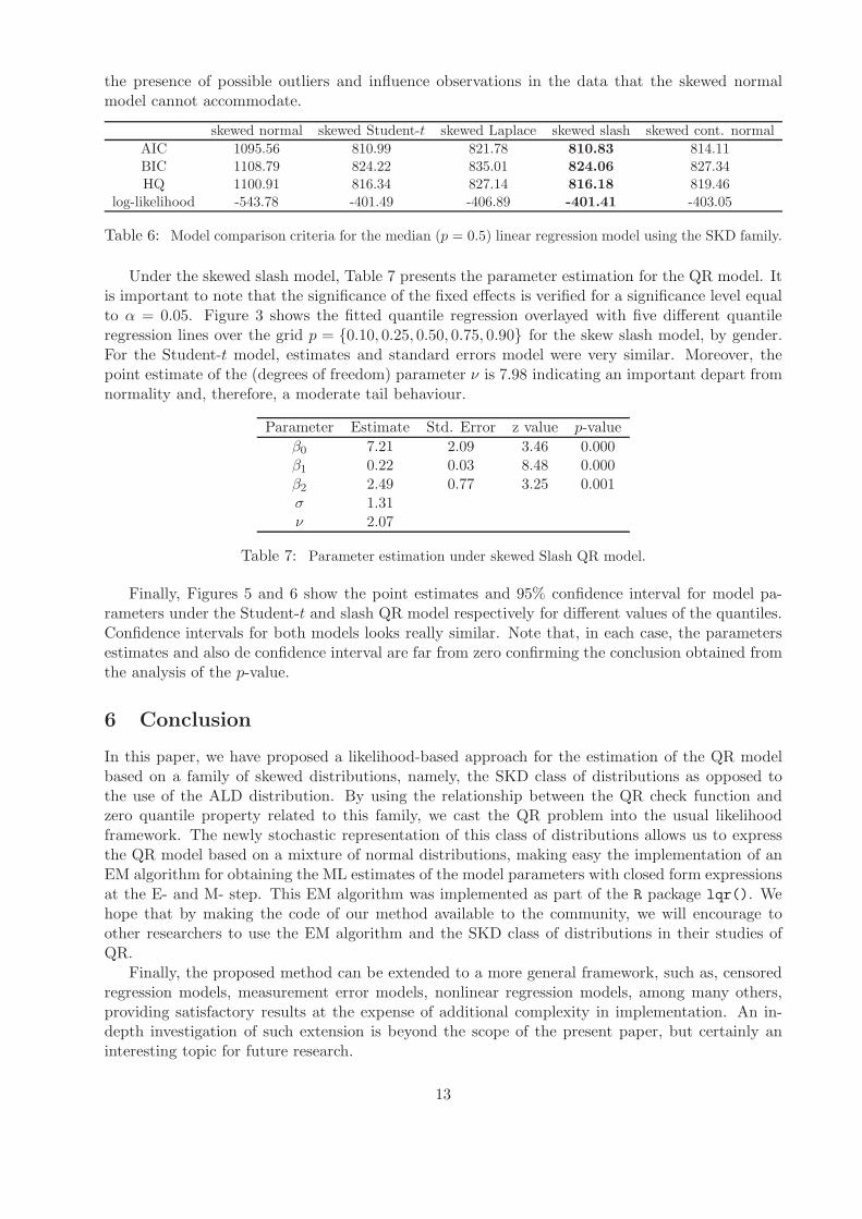
the presence of possible outliers and influence observations in the data that the skewed normalmodel cannot accommodate.

skewed normal skewed Student-t skewed Laplace skewed slash skewed cont. normal

AIC 1095.56 810.99 821.78 810.83 814.11BIC 1108.79 824.22 835.01 824.06 827.34HQ 1100.91 816.34 827.14 816.18 819.46

log-likelihood -543.78 -401.49 -406.89 -401.41 -403.05

Table 6: Model comparison criteria for the median (p = 0.5) linear regression model using the SKD family.

Under the skewed slash model, Table 7 presents the parameter estimation for the QR model. Itis important to note that the significance of the fixed effects is verified for a significance level equalto α = 0.05. Figure 3 shows the fitted quantile regression overlayed with five different quantileregression lines over the grid p = 0.10, 0.25, 0.50, 0.75, 0.90 for the skew slash model, by gender.For the Student-t model, estimates and standard errors model were very similar. Moreover, thepoint estimate of the (degrees of freedom) parameter ν is 7.98 indicating an important depart fromnormality and, therefore, a moderate tail behaviour.

Parameter Estimate Std. Error z value p-value

β0 7.21 2.09 3.46 0.000β1 0.22 0.03 8.48 0.000β2 2.49 0.77 3.25 0.001σ 1.31ν 2.07

Table 7: Parameter estimation under skewed Slash QR model.

Finally, Figures 5 and 6 show the point estimates and 95% confidence interval for model pa-rameters under the Student-t and slash QR model respectively for different values of the quantiles.Confidence intervals for both models looks really similar. Note that, in each case, the parametersestimates and also de confidence interval are far from zero confirming the conclusion obtained fromthe analysis of the p-value.

6 Conclusion

In this paper, we have proposed a likelihood-based approach for the estimation of the QR modelbased on a family of skewed distributions, namely, the SKD class of distributions as opposed tothe use of the ALD distribution. By using the relationship between the QR check function andzero quantile property related to this family, we cast the QR problem into the usual likelihoodframework. The newly stochastic representation of this class of distributions allows us to expressthe QR model based on a mixture of normal distributions, making easy the implementation of anEM algorithm for obtaining the ML estimates of the model parameters with closed form expressionsat the E- and M- step. This EM algorithm was implemented as part of the R package lqr(). Wehope that by making the code of our method available to the community, we will encourage toother researchers to use the EM algorithm and the SKD class of distributions in their studies ofQR.

Finally, the proposed method can be extended to a more general framework, such as, censoredregression models, measurement error models, nonlinear regression models, among many others,providing satisfactory results at the expense of additional complexity in implementation. An in-depth investigation of such extension is beyond the scope of the present paper, but certainly aninteresting topic for future research.

13

0.0 0.2 0.4 0.6 0.8 1.0

0.0

0.5

1.0

1.5

2.0

2.5

3.0

Student’s t model for p = 0.5 quantile

Theoretical HT(0.5, )quantiles

Sa

mp

le v

alu

es a

nd

enve

lop

e

0.0 0.5 1.0 1.5 2.0 2.5 3.0

01

23

45

Slash model for p = 0.5 quantile

Theoretical HSl(0.5, )quantiles

Sa

mp

le v

alu

es a

nd

enve

lop

e

Figure 4: Data analysis: Envelopes for the residuals after fitting the p = 0.5 skewed Student-tand skewed slash QR model.

Acknowledgements

The research of V.H. Lachos was supported by Grant 306334/2015-1 from Conselho Nacional de De-senvolvimento Cientıfico e Tecnologico (CNPq-Brazil) and by Grant 2014/02938-9 from Fundacaode Amparo a Pesquisa do Estado de Sao Paulo (FAPESP-Brazil). L.M. Castro acknowledgessupport from Grant FONDECYT 1130233 from the Chilean government and CONICYT-Chilethrough BASAL project CMM, Universidad de Chile. The research of C.E. Galarza was supportedby Grant 2015/17110-9 from FAPESP-Brazil. C. R. Cabral was supported by CNPq-Brazil (Grants308243/2012-9 and 447964/2014-3).

References

Akaike, H. (1974). A new look at the statistical model identification. IEEE Trans. Autom. Cont.,19, 379–397.

Andrews, D. F. & Mallows, C. L. (1974). Scale mixtures of normal distributions. Journal of theRoyal Statistical Society, Series B., 36, 99–102.

Barndorff-Nielsen, O. E. & Shephard, N. (2001). Non-gaussian ornstein–uhlenbeck-based modelsand some of their uses in financial economics. Journal of the Royal Statistical Society, Series B ,63, 167–241.

Barrodale, I. & Roberts, F. (1977). Algorithms for restricted least absolute value estimation.Communications in Statistics-Simulation and Computation, 6, 353–363.

Benites, L., Lachos, V. H. & Vilca, F. (2013). Likelihood based inference for quantile regressionusing the asymmetric Laplace distribution. Technical Report 15, Universidade Estadual deCampinas.

Cook, R. D. & Weisberg, S. (1994). An Introduction to Regression Graphics. Wiley, New York.

Dempster, A., Laird, N. & Rubin, D. (1977). Maximum likelihood from incomplete data via theEM algorithm. Journal of the Royal Statistical Society, Series B , 39, 1–38.

14

05

10

15

quantiles

β1

0.05 0.20 0.35 0.50 0.65 0.80 0.95

0.10

0.15

0.20

0.25

0.30

quantiles

β2

0.05 0.20 0.35 0.50 0.65 0.80 0.95

-10

12

34

5

quantiles

β3

0.05 0.20 0.35 0.50 0.65 0.80 0.95

0.0

0.5

1.0

1.5

2.0

quantilesσ

0.05 0.20 0.35 0.50 0.65 0.80 0.95

Point estimative and 95% CI for model parameters

Figure 5: Data analysis: Point estimates and 95% confidence interval for model parameters underthe skewed Student-t QR model.

05

10

15

quantiles

β1

0.10 0.25 0.40 0.55 00 0

quantiles

β2

0.10 0.25 0.40 0.55 00 0

−1

01

23

45

quantiles

β3

0.10 0.25 0.40 0.55 00 0

quantiles

σ

0.10 0.25 0.40 0.55 00 0

Point estimative and 95% CI for model parameters

Figure 6: Data analysis: Point estimates and 95% confidence interval for model parameters underthe skewed slash QR model.

15

Fernandez, C. & Steel, M. F. (1998). On bayesian modeling of fat tails and skewness. Journal ofthe American Statistical Association, 93(441), 359–371.

Galarza, C. E., Benites, L. & Lachos, V. H. (2015). lqr: Robust Linear Quantile Regression. Rpackage version 1.1.

Hannan, E. & Quinn, B. (1979). The determination of the order of an autoregression. Journal ofthe Royal Statistical Society, Series B , 41, 190–195.

Koenker, R. (2005). Quantile Regression, volume 38. Cambridge University Press.

Koenker, R. & G Bassett, J. (1978). Regression quantiles. Econometrica: Journal of the Econo-metric Society , 46, 33–50.

Koenker, R. W. & d’Orey, V. (1987). Algorithm as 229: Computing regression quantiles. Journalof the Royal Statistical Society. Series C (Applied Statistics), 36, 383–393.

Kottas, A. & Gelfand, A. E. (2001). Bayesian semiparametric median regression modeling. Journalof the American Statistical Association, 96, 1458–1468.

Kottas, A. & Krnjajic, M. (2009). Bayesian semiparametric modelling in quantile regression.Scandinavian Journal of Statistics, 36, 297–319.

Kozumi, H. & Kobayashi, G. (2011). Gibbs sampling methods for bayesian quantile regression.Journal of Statistical Computation and Simulation, 81, 1565–1578.

Lange, K. L. & Sinsheimer, J. S. (1993). Normal/independent distributions and their applicationsin robust regression. Journal of Computational and Graphical Statistics, 2, 175–198.

Louis, T. A. (1982). Finding the observed information matrix when using the EM algorithm.Journal of the Royal Statistical Society, Series B , pages 226–233.

Meilijson, I. (1989). A fast improvement to the EM algorithm on its own terms. Journal of theRoyal Statistical Society. Series B (Methodological), pages 127–138.

R Core Team (2014). R: A Language and Environment for Statistical Computing . R Foundationfor Statistical Computing, Vienna, Austria.

Schwarz, G. (1978). Estimating the dimension of a model. Annals of Statistics, 6(2), 461–464.

Tian, Y., Tian, M. & Zhu, Q. (2014). Linear Quantile Regression Based on EM Algorithm. Com-munications in Statistics - Theory and Methods, 43(16), 3464–3484.

Tibshirani, R. (1996). Regression shrinkage and selection via the lasso. Journal of the RoyalStatistical Society, Series B , pages 267–288.

Wichitaksorn, N., Choy, S. & Gerlach, R. (2014). A generalized class of skew distributions andassociated robust quantile regression models. Canadian Journal of Statistics, 42(4), 579–596.

Yu, K. & Moyeed, R. (2001). Bayesian quantile regression. Statistics & Probability Letters, 54,437–447.

Zhou, Y.-h., Ni, Z.-x. & Li, Y. (2014). Quantile Regression via the EM Algorithm. Communicationsin Statistics - Simulation and Computation, 43(10), 2162–2172.

16

Appendix

Proof of Lemma 1

Let H = |T0|, then we have that X = µ + σIH. In order to use the transformation method wedefine an auxiliar variable K = I, leading to I = K, H = (X−µ)/σK and thus |J| = 1/σK, where|J| represents the determinant of the Jacobian of the transformation. The joint distribution for Kand X can be computed as

f(k, x|µ, σ) = P (I = k)

σ|k| fH

(x− µ

σk

).

Using the fact that I and H are independent, then

f(k, x|µ, σ) =

2p(1− p)/σ fH (−2(1− p)(x− µ)/σ) ; x ≤ 0, k = −1/2(1 − p)

2p(1− p)/σ fH (2p(x− µ)/σ) ; x > 0, k = 1/2p

where P (I = k) = pIk = − 12(1−p) + (1 − p)Ik = 1

2p and H is a Half normal random variablewith pdf given by

fH(h) =

√2√πexp

−h2

2

Ih > 0.

Then, the pdf of X is obtained by marginalization, i.e.

f(x|µ, σ) = 2

[√2p(1− p)√

πσexp

−1

2

(x− µ

σ/2(1−p)

)2]

Ix ≤ 0

+2

[√2p(1− p)√

πσexp

−1

2

(x− µ

σ/2p

)2]

Ix > 0

= 2

[p φ

(x

∣∣∣∣µ,σ2

4(1 − p)2

)Ix ≤ 0+ (1− p)φ

(y

∣∣∣∣µ,σ2

4p2

)Ix > 0

],

concluding the proof.

Proof of Lemma 2

From Lemma 1, we have that Y |U = u ∼ SKN(µ, κ(u)1/2σ, p). Consequently, the marginal distri-bution of Y can be obtained from

f(y|µ, σ,ν) =∫ ∞

0

4p(1− p)√2πκ(u)σ2

exp

−2ρ2p

(y − µ

κ1/2(u)σ

)dH(u|ν)

corresponding to the pdf of the (4), concluding the proof.

Proof of Lemma 3

From the definition of check function ρp(·), the distance D = ρ(Y−µσ ) can be written asD = I2(

Y−µσ )

where I2 is a discrete random variable such that P (I2 = p − 1) = p and P (I2 = p) = 1 − p. LetI2 be independent of Y . Note that (Y − µ)/σ represents a standardized SKD random variable.

Therefore, from Lemma 2, it follows that Dd= I2κ(u)

1/2I|T0|. Finally, from the fact that T = I2×Iis a degenerate random variable such that P (T = 1/2) = 1, we conclude the proof.

17

Sample output from R package lqr()

--------------------------------------------------------------

Quantile Linear Regression using SKD family

--------------------------------------------------------------

Criterion = AIC

Best fit = Slash

Quantile = 0.5

--------------------------------

Model Likelihood-Based criterion

--------------------------------

Normal Student-t Laplace Slash C. Normal

AIC 1095.5632 810.9939 821.7857 810.8339 814.1112

BIC 1108.7963 824.2269 835.0188 824.0670 827.3443

HQ 1100.9173 816.3480 827.1398 816.1880 819.4654

loglik -543.7816 -401.4969 -406.8929 -401.4169 -403.0556

---------

Estimates

---------

Estimate Std. Error z value Pr(>|z|)

beta 1 7.21136 2.08532 3.45815 0.00054 ***

beta 2 0.22220 0.02619 8.48464 0.00000 ***

beta 3 2.48574 0.76500 3.24932 0.00116 **

---

Signif. codes: 0 "***" 0.001 "**" 0.01 "*" 0.05 "." 0.1 " " 1

sigma = 1.30806

nu = 2.0699

18