q&a research update

Third Quarter 2021Volume 6, Issue 3

When COVID-19 Reached the Corporate Bond Market

The Economic Effects of Changes in Personal Income Tax Rates

Banking Trends

Q&A

Research Update

Data in Focus

https://ideas.repec.org/s/fip/fedpei.html

https://www.philadelphiafed.org/

A publication of the Research Department of the Federal Reserve Bank of Philadelphia

Economic Insights features nontechnical articles on monetary policy, banking, and national, regional, and international economics, all written for a wide audience.

The views expressed by the authors are not necessarily those of the Federal Reserve.

The Federal Reserve Bank of Philadelphia helps formulate and implement monetary policy, supervises banks and bank and savings and loan holding companies, and provides financial services to depository institutions and the federal government. It is one of 12 regional Reserve Banks that, together with the U.S. Federal Reserve Board of Governors, make up the Federal Reserve System. The Philadelphia Fed serves eastern and central Pennsylvania, southern New Jersey, and Delaware.

Connect with UsWe welcome your comments at:[email protected]

E-mail notifications:www.philadelphiafed.org/notifications

Previous articles:https://ideas.repec.org/s/fip/fedpei.html

Twitter:@PhilFedResearch

Facebook:www.facebook.com/philadelphiafed/

LinkedIn:https://www.linkedin.com/company/philadelphiafed/

ContentsThird Quarter 2021 Volume 6, Issue 3

About the Cover

Second Bank of the United States

Opponents of the First Bank of the United States blocked reauthorization of the bank’s congressional charter in 1811, but their victory was short-lived: The War of 1812 triggered a financial crisis that necessitated the creation of the Second Bank of the United States. In 1824, the Second Bank’s permanent home opened on Chestnut Street. Modelled on the Parthenon, the temple built in Athens 2,500 years ago, the Second Bank of the United States features thick, imposing columns on top of a massive stepped platform. This building helped launch the Greek Revival style. However, the same forces that opposed the First Bank also opposed the Second. President Andrew Jackson, one of the bank’s biggest critics, vetoed the renewal of its charter in 1832. It would not be until 1913 that the U.S. yet again attempted to create a national bank, but this time it would be a central bank, not just a bank operating across state lines.

Illustration by Antonia Milas.

2 When COVID-19 Reached the Corporate Bond MarketAt the onset of the COVID-19 pandemic, several key markets faced serious trouble. Benjamin Lester takes a closer look at what happened in the corporate bond market, and at the Fed’s efforts to help.

25 Research UpdateAbstracts of the latest working papers produced by the Philadelphia Fed.

29 Data in FocusSouth Jersey Business Survey.

1 Q&A…with Benjamin Lester.

10 The Economic Effects of Changes in Personal Income Tax RatesHow do changes in personal income tax rates affect the economy? And does it matter who we tax, the wealthy or everyone else? Jonas Arias applies an empirical perspective to these and other questions.

18 Banking Trends: Is Small-Business Lending Local? The rise of business cards has undercut the dominance of local banks in small- business lending, though, as Jim DiSalvo explains, small banks still compete in making relationship loans.

Patrick T. HarkerPresident and Chief Executive Officer

Michael DotseyExecutive Vice President and Director of Research

Adam SteinbergManaging Editor, Research Publications

Brendan BarryData Visualization Manager

Antonia MilasGraphic Design/Data Visualization Intern

ISSN 0007–7011

https://ideas.repec.org/s/fip/fedpei.html

mailto:PHIL.EI.Comments%40phil.frb.org?subject=

http://www.philadelphiafed.org/notifications

https://twitter.com/PhilFedResearch

http://www.facebook.com/philadelphiafed/

https://www.linkedin.com/company/philadelphiafed/

https://www.linkedin.com/company/philadelphiafed/

https://www.philadelphiafed.org/our-people/benjamin-lester


https://www.philadelphiafed.org/our-people/jonas-arias

https://www.philadelphiafed.org/our-people/jim-disalvo

https://www.philadelphiafed.org/our-people/patrick-t-harker

https://www.philadelphiafed.org/our-people/michael-dotsey

mailto:Adam.Steinberg%40phil.frb.org?subject=

mailto:[email protected]

Federal Reserve Bank of PhiladelphiaResearch Department

Q&A2021 Q3 1

Benjamin Lester

Benjamin Lester is a senior economic advisor and economist at the Philadelphia Fed. He grew up in suburban Philadelphia and first encountered economics while a student at the Lawrenceville School. He earned his bachelor’s in economics from Cornell in 2002 and his doctor- ate from the University of Pennsylvania in 2007. After teaching at the University of Western Ontario for four years, he joined the Research Department of the Philadelphia Fed, where he specializes in studying how market frictions affect real-life markets.

What led you to become an economist?I always loved mathematics. I got to Cornell thinking, “I’m good at math, so I’ll major in it.” But then I saw people who are really good at math, and I thought, “I’m not going to be a mathematician.” That’s when I started taking economics classes. As an economist, you’re not a pure mathemati-cian, but you use applied quantitative skills to answer interesting questions.

Tell us about your interest in market frictions.In the classic model of supply and demand, no one asks, who traded with who? How did they find each other? How did they settle on that price? That’s all brushed under the rug. But think about the housing market. You can’t go to the housing market and say, houses are selling at this price and I’ll take one. You have to see a house, make an offer, maybe your offer is rejected or maybe the seller makes a counteroffer. The terms of trade are deter-mined bilaterally. It’s not as if there’s a price for a house.

And it’s not as if you know everything about the house. Maybe the furnace is on its last legs, or the neighbors are loud. Knowing that the owner knows more than you do, how does this affect your offer?

Some of these frictions are associated with what economists call search frictions, which refers to the idea that it’s often hard—or it takes time—for buyers and sell-ers who are natural trading partners to find each other and negotiate a price. And where there are search frictions, there are often also information frictions, which oc-cur when one side of a transaction knows more than the other.

As I studied these two frictions, I realized that they fit together. Solving a model with search frictions requires characterizing the terms of trade between two people. Meanwhile, much of the literature on information frictions starts with understanding how two people with different information may or may not trade.

But hasn’t the digital revolution done away with many of these frictions? After all, thanks to digital technology we are swamped with information, and finding a counterparty should be much easier.

Not always. I’ll give you an example. De-cades ago, stock exchanges turned equities into a fairly frictionless market. If you want to buy stock in IBM, give me three seconds, I’ll check my computer, I’ll tell you the price, and I’ll trade at that price. But the corporate bond market is not like that at all. If you want to buy a corporate bond, you call up a dealer and say, “I’m looking for this particular bond with this maturi-ty.” And they might say, “OK, let me see if I can find that bond. I’ll get back to you.” Maybe you buy at their price, or maybe you call another dealer. That falls into the search model I’ve been working on, where it takes time to find and negotiate with a counterparty. For some reason, older technologies seem to be valuable to some market participants.

You conclude your article for Economic Insights by writing, “the Fed’s March 23 announcement of the SMCCF… calmed investors and reduced with-drawals from funds.”1 That sounds to me like a psychological response. Where does psychology fit into the models of market frictions?When I write about calming the market, I’m thinking about agents who are rational and forward-looking. If I’m a perfectly rational, forward-looking agent, I have reason to be concerned at the beginning of a crisis. I’m not sure who’s going to buy my asset. Or there’s a lot of uncertainty about the quality of this asset. I’m wor-ried that maybe the rest of the market knows something I don’t about my asset. That might make me want to sell it right now. If the Fed says, “We’re going to buy these assets,” it lessens those worries that derive from information frictions. I use terms that have a psychological interpre-tation, but I use them within a perfectly rational paradigm. In behavioral econo-mics models, people are systematically biased. But I’m thinking about a world where they’re not biased, and policies can resolve inefficiencies that come from frictions.

Notes1 The Secondary Market Corporate Credit Facility allows the Fed, for the first time, to directly purchase investment-grade corporate bonds issued by U.S. companies.

Q&A…with Benjamin Lester, a senior economic advisor and economist here at the Philadelphia Fed.

https://www.philadelphiafed.org/the-economy



2 Federal Reserve Bank of PhiladelphiaResearch Department

When COVID-19 Reached the Corporate Bond Market2021 Q3

As the economic implications of the COVID-19 crisis became clear, financial markets across the globe entered a period of distress. As asset prices fell, investors rushed to liquidate

large portions of their portfolios in a “dash for cash.” However, in several key markets, investors found it difficult to find dealers that would buy these assets at a reasonable price.

One market that was under severe distress was the $10 trillion U.S. corporate bond market. This market, which is the primary source of funding for large U.S. corporations, was bound to play an important role during the pandemic, since firms in a number of hard-hit sectors—such as travel, hospitality, and entertainment— would surely need to borrow in order to survive significant declines in revenue. However, by the middle of March 2020, the corporate bond market was “basically broken,” prompting the Federal Reserve to intervene in an unprecedented fashion.1

In this article, I describe the deterioration in trading conditions in the corporate bond market at the onset of the pandemic, and the likely causes of this deterioration. Then, I describe how the Federal Reserve intervened, and how the market responded. Finally, I pose a few questions for policymakers to consider before the next crisis.

When COVID-19 Reached the Corporate Bond Market

Benjamin LesterSenior Economic Advisor and EconomistFeDeral reSerVe BaNk OF PhIlaDelPhIa

The views expressed in this article are not necessarily those of the Federal Reserve.

Photo: Aimur Kytt/iStock

We investigate how the pandemic affected the corporate bond mar-ket, and how the Fed responded.





When COVID-19 Reached the Corporate Bond Market2021 Q3 3

500

100150200250

500

750

1000

1250

AAA

HY

Feb 19

Mar 23

Mar 18

Trouble in the Corporate Bond MarketAfter reaching an all-time high on Feb- ruary 19, 2020, U.S. equity markets began a rapid decline in early March as the COVID- 19 virus spread throughout the world.2 Soon after, the sell-off extended beyond equity markets and into a number of key credit markets.

In the corporate bond market, trading volume surged by more than 50 percent, reflecting a sharp increase in selling pressure (Figure 1). As a result, corporate bond prices began to fall and interest rates on corporate bonds—which move in the opposite direction as prices—rose sharply. In Figure 2, I plot the changes in interest rates for two types of corporate bonds relative to a risk-free benchmark. One line represents the spread between the interest rate on relatively safe corpo-rate bonds (rated investment grade) and the interest rate on a risk-free security (a Treasury). The other line depicts the

corresponding spread for riskier, high-yield corporate bonds (rated below investment grade). We see that interest rates on both relatively safe and somewhat riskier corporate debt spike substantially relative to the risk-free benchmark: The credit spread for safe bonds increased by about 150 basis points at the height of the crisis, while the corresponding spread for high-yield corporate debt increased more than 500 basis points.

Although it’s painful for owners of corporate bonds, as well as for firms that need to borrow, there is nothing neces-sarily wrong with an increase in selling pressure and a subsequent fall in prices. These are simply signs of an increase in the supply of bonds for sale without a commensurate increase in demand. However, reports emerging from the cor-porate bond market last spring signaled a more fundamental problem: The market

was becoming illiquid, in the sense that it was becoming harder and more costly for investors to trade at prevailing prices.

In a recent paper, five other economists and I attempted to quantify the deteriora-tion in market liquidity in the corporate bond market during the COVID-19 crisis.3 We measured the cost that dealers were charging for customers to buy and sell corporate bonds—also known as the bid-ask spread—under two trading arrangements.4 The first type of trade, called a risky- principal trade, occurs when a dealer trades directly and immediately with a customer: The dealer purchases bonds from a customer who wants to sell, ab-sorbing the bonds onto its own balance sheet; subsequently, the dealer draws down its inventory of bonds by selling to a customer who wants to buy. The second type of trade, called a riskless-principal or agency trade, occurs when a dealer

F I G U R E 1

Trading Volume Nearly Doubled from the Beginning to the End of March 2020This reflects a surge in selling pressure. Trading volume, billions of dollars, February 14 to May 30, 2020

Source: TraCe corporate bond data set combined with the Mergent Fixed Income Securities Database (FISD).

Note: aaa is the highest possible rating that can be assigned to a bond. High-yield bonds, also known as

“junk” bonds, pay higher interest rates because they have a lower credit rating than investment-grade bonds.

Source: ICe Data Indices (ICe BofA aaa U.S. Corporate Index Option-Adjusted Spread and ICe BofA U.S. High Yield Index Option-Adjusted Spread, both available from Federal Reserve Economic Data [FreD], St. Louis Fed).

F I G U R E 2

Before the Fed’s Interventions, Interest Rates on Bonds Surged as Their Prices Fell The decline in prices affected both lower- and highly rated bonds.Credit spread between corporate bonds and a risk-free security (a Treasury) in basis points, high-yield (HY) bonds and aaa-rated bonds, February 14 to May 30, 2020

Movingaverage

Dollar trading volume

Raw

10

5

0

15

20

25

Feb 19

Mar 23Mar 18





What Caused the Deterioration in Market Liquidity?While a variety of factors contributed to the sudden evaporation of liquidity in the corporate bond market in March 2020, two simultaneous developments appear to have played an outsized role. First, there was a dramatic increase in the quantity of bonds customers were trying to sell—that is, there was a surge in the demand for liquidity. At the same time, there was a decrease in dealers’ willingness to absorb these bonds onto their own balance sheets—that is, there was a reduction in the supply of liquidity.

On the demand side, the ramifications of the pandemic for corporate profits, and the expectation that some corporate debt would be downgraded to a riskier rating, motivated many investors to decrease their exposure to the corporate bond market. Leading the way were mutual funds that invest in corporate bonds; these funds were forced to sell a portion of their corporate bond holdings as in-vestors pulled out their money in droves. Economists Antonio Falato of the Federal Reserve, Itay Goldstein of the University of Pennsylvania, and Ali Hortaçsu of the University of Chicago report that the average corporate bond fund experienced cumulative outflows of approximately 9 percent of net asset value in February and March of 2020.

acts as a middleman and simply finds an-other customer to take the other side of the trade. These trades are typically less attractive for customers, since they have to wait while a dealer finds a counterpar-ty, but more attractive for dealers, since they don’t have to use their own balance sheet to facilitate the trade.

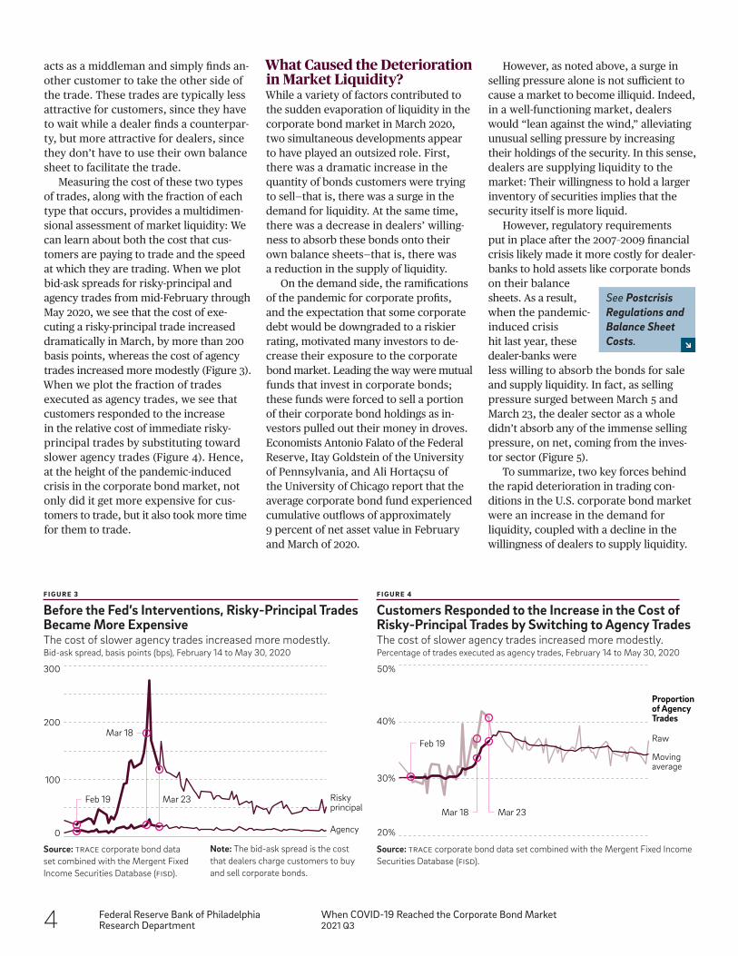
Measuring the cost of these two types of trades, along with the fraction of each type that occurs, provides a multidimen-sional assessment of market liquidity: We can learn about both the cost that customers are paying to trade and the speed at which they are trading. When we plot bid-ask spreads for risky-principal and agency trades from mid-February through May 2020, we see that the cost of exe-cuting a risky-principal trade increased dramatically in March, by more than 200 basis points, whereas the cost of agency trades increased more modestly (Figure 3). When we plot the fraction of trades executed as agency trades, we see that customers responded to the increase in the relative cost of immediate risky- principal trades by substituting toward slower agency trades (Figure 4). Hence, at the height of the pandemic-induced crisis in the corporate bond market, not only did it get more expensive for customers to trade, but it also took more time for them to trade.

However, as noted above, a surge in selling pressure alone is not sufficient to cause a market to become illiquid. Indeed, in a well-functioning market, dealers would “lean against the wind,” alleviating unusual selling pressure by increasing their holdings of the security. In this sense, dealers are supplying liquidity to the market: Their willingness to hold a larger inventory of securities implies that the security itself is more liquid.

However, regulatory requirements put in place after the 2007–2009 financial crisis likely made it more costly for dealer- banks to hold assets like corporate bonds on their balance sheets. As a result, when the pandemic- induced crisis hit last year, these dealer-banks were less willing to absorb the bonds for sale and supply liquidity. In fact, as selling pressure surged between March 5 and March 23, the dealer sector as a whole didn’t absorb any of the immense selling pressure, on net, coming from the inves-tor sector (Figure 5).

To summarize, two key forces behind the rapid deterioration in trading conditions in the U.S. corporate bond market were an increase in the demand for liquidity, coupled with a decline in the willingness of dealers to supply liquidity.

F I G U R E 3

Before the Fed’s Interventions, Risky-Principal Trades Became More ExpensiveThe cost of slower agency trades increased more modestly.Bid-ask spread, basis points (bps), February 14 to May 30, 2020


Note: The bid-ask spread is the cost that dealers charge customers to buy and sell corporate bonds.

F I G U R E 4

Customers Responded to the Increase in the Cost of Risky-Principal Trades by Switching to Agency TradesThe cost of slower agency trades increased more modestly.Percentage of trades executed as agency trades, February 14 to May 30, 2020


0

100

200

300

Agency

Risky principal

Feb 19 Mar 23

Mar 18Feb 19

Mar 23Mar 18

30%

20%

40%

50%

Movingaverage

Proportion of Agency Trades

Raw

See Postcrisis Regulations and Balance Sheet Costs.





When combined, these two forces can create a dangerous “illiquidity spiral”: As assets get harder to sell to dealers, they become less valuable and riskier for investors to hold. Then, as investors’ appetite for these bonds dwindles, dealers become even more concerned about buying them, since dealers know that if they buy these bonds, they have to either leave the bonds on their balance sheet for a long time or sell them at a loss. Facing the prospects of such a spiral—with rapidly falling bond prices and, hence, rapidly increasing borrowing rates for U.S. firms—the Federal Reserve decided to intervene.

The Fed IntervenesThe Fed responded to the turmoil in financial markets with a variety of measures (Figure 6). Early in the crisis, on March 3, the Federal Open Market Committee (FOMC), using its traditional lever for easing monetary policy, dropped the target for the fed funds rate by 50 basis points. Then, on March 15, the FOMC decreased the target rate by another 100 basis points, to essentially zero, and announced that it would use its full range of tools to support the flow of credit to households and businesses.

Among the many tools that the Fed chose to employ, three policies were most likely to affect liquidity in the corporate bond market, either by reducing investors’ desire to sell their bonds or by increasing dealers’ willingness to absorb these bonds onto their balance sheets.

First, the Fed assumed the role of “lender of last resort” by in- troducing a number of facilities that made it easier and less costly for dealers to borrow funds. In particular, on the evening of March 17, the Fed announced that it would revive the Primary Dealer Credit Facility (PDCF). Originally introduced in 2008, the PDCF offered collateralized overnight term lending to primary dealers starting on March 20.5 By allowing dealers to borrow against a variety of assets on their balance sheets, including

F I G U R E 5

Before the Fed’s Intervention, Dealer Banks Were Reluctant to Buy Bonds This fueled the liquidity crisis.Cumulative inventory of corporate bonds held by dealer banks, billions of dollars, February 19 to May 30, 2020

Source: FINra market sentiment tables.

F I G U R E 6

Corporate Bond Market Timeline During the COVID-19 Crisis

0

−10

10

30

50

−20

20

40

60

Feb 19

Mar 23Mar 18

March

April

3 Mar The fomc dropped fed funds target rate by 50 basis points (bps)

The fomc dropped fed funds target rate by an 15 Mar additional 100 bps, to essentially zero

The Fed announced it would revive the Primary 17 Mar Dealer Credit Facility (pdcf)18 Mar Markets began trading again

1 Apr The Fed temporarily exempted both Treasury securities and reserves from the supplementary leverage ratio (slr)

20 Mar The pdcf began overnight term lending to primary dealers

23 Mar The Fed announced the Primary and Secondary Market Corporate Credit Facilities (pmccf and smccf, respectively)

9 Apr The Fed expanded the pmccf and smccf programs in size and scope

12 May The smccf began buying corporate bonds





Movingaverage

Dollar trading volume

Raw

10

5

0

15

20

25

May 12

Mar 23

Apr 9

Finally, to relax dealers’ balance sheet constraints and reduce the cost of provid-ing intermediation services, on April 1 the Fed temporarily exempted both Treasury securities and reserves from the supple-mentary leverage ratio (SLR).7 Although this exemption was primarily intended to increase liquidity in the Treasury market, the effects would clearly extend to the cor-porate bond market, since dealers would be more willing to absorb corporate bonds onto their balance sheets if there were less risk of violating the SLR.

How Markets Responded to the Fed’s Intervention After the Fed’s various interventions were announced, the price of corporate bonds rebounded and credit spreads fell significantly, with an especially noticeable improvement after the March 23 announcement of the corporate credit facilities (Figure 2). At the same time, measures of market liquidity recovered. For example,

corporate bonds, the PDCF was designed to reduce the costs associated with holding inventory and intermediating transactions between customers.

Second, to ease the panic and restore liquidity in the corporate bond market, on March 23 the Fed announced the Primary and Secondary Market Corporate Credit Facilities (PMCCF and SMCCF, respectively). According to the initial announcement, these facilities would allow the Fed, for the first time, to directly purchase investment- grade corporate bonds issued by U.S. companies, as well as exchange-traded funds (ETFs) that invested in similar assets. On April 9, these corporate credit facilities were expanded in both size and scope, allowing the Fed to also purchase some lower-rated corporate debt.6 By stepping in as a (potentially large) buyer of corporate bonds, the Fed could ameliorate the risk of the illiquidity spiral described above by reducing investors’ desire to sell their bonds and increasing dealers’ willingness to buy them.

F I G U R E 1 ( R E V I S I T E D)

After the Fed’s Interventions, Trading Volume in Corporate Bonds Stabilized… This reflects an easing in selling pressure.Trading volume, billions of dollars, February 14 to May 30, 2020


Source: ICe Data Indices (ICe BofA aaa U.S. Corporate Index Option-Adjusted Spread and ICe BofA U.S. High Yield Index Option-Adjusted Spread, both available on Federal Reserve Economic Data [FreD], St. Louis Fed).


…Interest Rates on Bonds Fell as Their Prices Stabilized…Prices recovered for both lower- and highly rated bonds, but not fully.Credit spread between corporate bonds and a risk-free security (a Treasury) in basis points, high-yield (HY) bonds and aaa-rated bonds, February 14 to May 30, 2020

the cost of trading immediately via risky- principal trades declined by more than 100 basis points (Figure 3), and there was a corresponding shift away from slower agency trades (Figure 4). Perhaps the starkest evidence of an improvement in liquidity provision comes from the sharp change in dealers’ willingness to absorb inventory onto their balance sheets (Figure 5). Between March 18 and the end of May, dealers increased their net holdings of corporate bonds by more than $60 billion, thus doubling their precrisis holdings.

These observations establish the coincidence of key interventions and improvements in market liquidity, but they do not establish that the Fed’s interventions caused an improvement in market liquidity. To study the causal relationship between policy and market conditions more closely, my coauthors and I exploited the eligibility requirements of the Fed’s corporate credit facilities to perform a difference-in- differences regression.

500

100150200250

500

750

1000

1250

AAA

HY

Mar 23

May 12

Apr 9





When the SMCCF was announced, the term sheet specified certain eligibility requirements for bonds to be purchased by the Fed. These requirements included an investment-grade credit rating and a maximum maturity of five years. The difference-in- differences approach attempts to isolate the causal effect of the Fed’s bond-purchasing program by studying the differential behavior of bid-ask spreads before and after the announcement of the SMCCF for two groups of bonds: those eligible for purchase (the treatment group) and those ineligible (the control group). We found that immediately after the March 23 announcement, bid-ask spreads for risky-principal trades declined by about 50 basis points more for bonds that were eligible to be purchased by the SMCCF than for otherwise similar but ineligible bonds. Later, when the program was expanded in both size and scope—and other policies were introduced, such as the relaxation of the SLR—the cost of trading all bonds declined.

Interestingly, despite the significant improvements in the corporate bond market after the Fed’s interventions, trading conditions did not fully return to their precrisis levels. Even in June 2020, the cost of risky-principal trades and the fraction of agency trades remained above the levels observed in January 2020. Hence, it appears that market liquidity did not fully recover, even after markets had calmed.

Lingering QuestionsGiven the expansive approach of the Federal Reserve during the height of the mid-March turmoil—in which a variety of distinct interventions were announced and implemented in a short period of time—it’s difficult to isolate the effect of each program, and thus difficult to assess which interventions were most effective and why. However, policymakers need to understand the frictions that generated illiquidity and identify the policies that eased these frictions. In particular, what are the conditions that can generate large, sudden surges in selling pressure after an adverse event such as the outbreak of COVID-19? And which regulations prevent dealers from absorbing this selling pressure?

Though economists have not fully answered these questions, recent research is providing some clues. For one, the growing popularity of bond mutual funds over the last decade has enabled larger, more immediate surges in selling pressure during times of distress, since these funds are forced to liquidate their positions when investors withdraw their funds.8 Hence, the Fed’s March 23 announcement of the SMCCF—which calmed investors and re-duced withdrawals from funds—appears to have played a key role in halting (and even reversing) the illiquidity spiral that began in the second week of March.9

However, market liquidity had not fully recovered even months after the initial panic had passed, suggesting that lingering and important frictions could prevent dealers from “leaning against the wind” in future crises. Understanding the precise nature of these frictions and evaluating whether their costs (in terms of market liquidity) outweigh their benefits (in terms of financial stability) remain top priorities for future research.


…Risky-Principal Trades Became Cheaper…This is a sign of improving market liquidity.Bid-ask spread, basis points, February 14 to May 30, 2020



…Fraction of Faster Risky-Principal Trades Increased…This is another sign of improving market liquidity.Percentage of trades executed as agency trades, February 14 to May 30, 2020



…& Dealers Absorbed Assets onto Their Balance SheetsCumulative inventory of corporate bonds held by dealer banks, billions of dollars, February 19 to May 30, 2020

Source: FINra market sentiment tables.

0

100

200

300

Agency

Risky principal

Mar 23

Apr 9 May 12

May 12Mar 23

Apr 9

30%

20%

40%

50%

Movingaverage

Proportion of Agency Trades

Raw

0

−10

10

30

50

−20

20

40

60

May 12

Apr 9

Mar 23





Notes1 See Idzelis (2020).

2 For example, between March 5 and March 23, the S&P 500 index declined by more than 25 percent.

3 See Kargar et al. (forthcoming).

4 The price a dealer is willing to pay for an asset is called the “bid,” while the price at which a dealer is willing to sell an asset is called the

“ask.” Hence, the difference or “spread” between the two prices is a natural measure of how much it costs to trade, and it is often used as a metric for market liquidity.

5 Primary dealers are trading counterparties of the New York Fed that intermediate markets for government securities, along with other fixed- income securities, including corporate and municipal debt.

6 Although announced on March 23, these facilities did not begin purchasing bonds until May 12.

7 These exemptions were extended first to bank holding companies and later to commercial bank subsidiaries.

8 See Falato et al. (2020), Ma et al. (2020), and Haddad et al. (forthcoming).

9 Boyarchenko et al. (2020) estimate that about one-third of the market’s recovery can be attributed to the announcement of the PMCCF and SMCCF alone.

10 Bao et al. (2018) find that banks subject to the Volcker rule are less willing to provide liquidity during episodes in which investors are suddenly forced to sell corporate bonds.

11 Also see Adrian et al. (2017) and Anderson et al. (2017).

12 See Bao et al. (2018), Dick-Nielsen et al. (2019), Bessembinder et al. (2018), and Choi et al. (2019).

Postcrisis Regulations and Balance Sheet CostsAfter the 2007–2009 financial crisis, a number of new regulations were introduced to strengthen the resilience of the banking sector. However, some of these regulations have arguably increased the cost for dealers of holding assets on their balance sheets and thus could have important consequences for liquidity provision in dealer-intermediated financial markets.

Perhaps the most important set of regulations is the 2010 Basel III framework, devised by the Basel Committee on Banking Supervision (BCBS). This frame-work includes both enhanced capital and new leverage-ratio requirements. For example, the BCBS introduced a liquidity coverage ratio (lCr), which requires banks to have enough high-quality liquid assets to cover potential outflows over a hypothetical 30-day period in which markets are experiencing stress. The Basel III framework also includes limits on leverage, including a supplementary leverage ratio (Slr) requirement, which ensures that a bank holding company’s tier 1 capital is sufficiently large relative to its total leverage exposure, including both on-balance-sheet and off-balance-sheet exposures. In short, these types of requirements imply that banks need to hold more capital as their balance sheets expand, which is costly.

Another important set of regulations for U.S. dealer-banks derives from the Dodd-Frank Wall Street Reform and Consumer Protection Act of 2010, which includes the so-called Volcker rule. Among other things, this rule prohibits banking entities from engaging in proprietary trading—that is, trading activities with their own accounts. Despite an exception for trading activities related to intermediating, or “market-making,” in practice it can be difficult to distinguish between proprietary trading and market-making. Hence, if the Volcker rule reduced the incentive of regulated dealers to buy and sell bonds—since financial penalties would be incurred if this activity were deemed proprietary trading—then the Volcker rule could be responsible for decreased liquidity.10

In the academic literature, there are differing views on whether (and to what extent) these new regulations caused a decline in liquidity in the U.S. corporate bond market. In their study of a variety of price-based measures of market liquidity during “normal” trading conditions, University of California, Berkeley, economist Francesco Trebbi and Columbia Business School economist Kairong Xiao found very little effect of postcrisis regulations.11 However, there is consider- able evidence that after the implementation of these new regulations, markets appear less liquid (or less resilient) during periods of intense selling pressure. For example, several studies examine dealers’ behavior in response to a large surge in selling pressure for nonfundamental reasons, such as when a bond must be sold by index funds because its maturity falls below a certain threshold.12 Collectively, these studies find that the impact on prices during these episodes increased after the introduction of postcrisis regulations, and the effect is more pronounced at dealer-banks that are subject to regulation than at those that are exempt.





ReferencesAdrian, Tobias, Michael Fleming, Or Shachar, and Erik Vogt. “Market Liquidity After the Financial Crisis,” Annual Review of Financial Economics, 9 (2017), pp 43–83, https://doi.org/10.1146/annurev- financial-110716-032325.

Anderson, Mike, and René M. Stulz. “Is Post-crisis Bond Liquidity Lower?” National Bureau of Economic Research Working Paper 23317 (2017), https://doi.org/10.3386/w23317.

Bao, Jack, Maureen O’Hara, and Xing (Alex) Zhou. “The Volcker Rule and Market Making in Times of Stress,” Journal of Financial Economics, 130 (2018), pp. 95–113, https://doi.org/10.1016/j.jfineco.2018.06.001.

Bessembinder, Hendrik, Stacey Jacobsen, William Maxwell, and Kumar Venkataraman. “Capital Commitment and Illiquidity in Corporate Bonds,” Journal of Finance, 73 (2018), pp. 1615–1661, https://doi.org/10.1111/jofi.12694.

Boyarchenko, Nina, Anna Kovner, and Or Shachar. “It’s What You Say and What You Buy: A Holistic Evaluation of the Corporate Credit Facilities,” Federal Reserve Bank of New York Staff Report 935 (2020).

Choi, Jaewon, and Yesol Huh. “Customer Liquidity Provision: Implications for Corporate Bond Transaction Costs,” Finance and Economics Discussion Series 2017-116, Federal Reserve Board of Governors, Washington, D.C. (2018), https://doi.org/10.17016/FEDS.2017.116.

Dick-Nielsen, Jens, and Marco Rossi. “The Cost of Immediacy for Corpo-rate Bonds,” Review of Financial Studies, 32:1 (2019), pp. 1–41, https://doi.org/10.1093/rfs/hhy080.

Falato, Antonio, Itay Goldstein, and Ali Hortaçsu. “Financial Fragility in the COVID-19 Crisis: The Case of Investment Funds in Corporate Bond Markets,” Becker Friedman Institute Working Paper 2020-98 (2020).

Haddad, Valentin, Alan Moreira, and Tyler Muir. “When Selling Becomes Viral: Disruptions in Debt Markets in the COVID-19 Crisis and the Fed’s Response,” Review of Financial Studies (forthcoming).

Idzelis, Christine. “The Corporate Bond Market Is ‘Basically Broken,’ Bank of America Says,” Institutional Investor, March 19, 2020.

Kargar, Mahyar, Benjamin Lester, David Lindsay, Shuo Liu, Pierre-Olivier Weill, and Diego Zúñiga. “Corporate Bond Liquidity During the Covid-19 Crisis,” Review of Financial Studies (forthcoming).

Ma, Yiming, Kairong Xiao, and Yao Zeng. “Mutual Fund Liquidity Trans-formation and Reverse Flight to Liquidity,” Columbia Business School Working Paper (2020).

Trebbi, Francesco, and Kairong Xiao. “Regulation and Market Liquidity,” Management Science, 65:5 (2017), pp. 1949–2443, https://doi.org/10.1287/ mnsc.2017.2876.



https://www.annualreviews.org/doi/10.1146/annurev-financial-110716-032325

https://www.annualreviews.org/doi/10.1146/annurev-financial-110716-032325

https://doi.org/10.3386/w23317

https://doi.org/10.1016/j.jfineco.2018.06.001

https://doi.org/10.1111/jofi.12694

https://doi.org/10.1111/jofi.12694

https://doi.org/10.17016/FEDS.2017.116

https://doi.org/10.1093/rfs/hhy080

https://doi.org/10.1093/rfs/hhy080

https://doi.org/10.1287/mnsc.2017.2876

https://doi.org/10.1287/mnsc.2017.2876


The Economic Effects of Changes in Personal Income Tax Rates2021 Q3

The Economic Effects of Changes in Personal Income Tax RatesWe apply an empirical perspective to understand the macroeconomic consequences of changes in personal income taxes.

The personal federal income tax as we know it today was adopted in 1913 after a protracted political and judicial process

that culminated in the ratification of the 16th Amendment.1 Within 60 years, most U.S. states had implemented a personal state income tax as well, and the federal government had added the Social Security payroll tax.2 Throughout this process and ever since, personal income taxation has been an intensely debated issue in policy and academic circles. But even after all these debates, experts still disagree about exactly how personal income tax rates affect individual economic behavior and macroeco-nomic outcomes.

Some empirical studies find that economic activity responds to cuts in marginal tax rates but not to cuts in average tax rates. Other

studies find that both marginal and average tax rates affect the economy. Likewise, some em-pirical evidence shows that tax cuts for workers with high earnings lead to sizable changes in personal income, and also that such cuts are more effective in stimulating economic activity in the near term than tax cuts for workers with lower earnings. Other research, however, argues the opposite.3

This lack of consensus in the empirical litera-ture complicates the design of not only fiscal policy reforms aimed at achieving long-run economic growth but also fiscal policy actions aimed at stimulating short-run economic activity.

To address these issues, we need to tackle a few

Jonas AriasSenior EconomistFeDeral reSerVe BaNk OF PhIlaDelPhIa


See Marginal vs. Average Personal Income Tax Rates.

Photo: Skyhobo/iStock



https://www.philadelphiafed.org/our-people/jonas-arias


The Economic Effects of Changes in Personal Income Tax Rates2021 Q3 11

questions. Do changes in tax policy operate by means of supply side effects associated with marginal tax rates—by, for example, fostering incentives to work or to take on entrepreneurial opportunities? Or do they operate through demand effects associated with average tax rates—by, for example, fostering consumption among individuals who now have more after-tax income to spend? Does tax policy operate through trickle-down effects, whereby cutting marginal tax rates for those at the top of the income distribution leads to broad economic gains? Or does it operate through bottom-up effects by stimulating people outside the top of the income distribution to work longer hours or join the labor force, raising their incomes and inducing economic growth?

In this article, I examine these ques-tions from an empirical perspective and analyze how changes in personal income taxes affect economic activity.

Economic Consequences of Changes in Marginal RatesAssessing the economic consequences of changes in marginal tax rates is chal-lenging due to two features of income taxation. First, the marginal tax rate paid by an individual depends on their level of income. Second, there are three types of personal income taxes: federal income taxes, state income taxes, and Social Security payroll taxes.

Because marginal tax rates depend on the level of income, there is no one marginal tax rate for everyone. Instead, there’s a distribution of rates across the popula-tion. And because we have three types of income taxes, there are three distributions: one for federal income marginal tax rates, one for state income marginal tax rates, and one for payroll marginal tax rates. But, to analyze the aggregate effects of tax changes, it is useful to rely on a single, succinct measure that allows us to study what happens within the economy when any of these distributions change.

Economists’ primary summary indi-cator of marginal tax rates is the overall average marginal tax rate—that is, the sum of federal, state, and payroll tax rates across taxpayers weighted by their income relative to the total income of the population.6 This rate corresponds to

Marginal vs. Average Personal Income Tax RatesThe marginal tax rate is the tax rate im-posed on an additional dollar of adjusted gross income.

Adjusted gross income is defined as gross income (which includes wages and other forms of income, such as dividends, capital gains, and business income) minus adjust-ments such as interest paid on student loans and contributions to a retirement account.

Under the current federal tax code, the marginal tax rate is graduated, increasing with each higher level of income (Figure 1). The same holds for most state income taxes, albeit the rates are lower and differ by states. In contrast, the marginal rate on the Social Security payroll tax, though graduated, decreases with income.4

For ease of exposition, let’s ignore state income and payroll taxes. Now imagine an individual with an income of $72,400 (corresponding to the tax year 2020) who uses the standard deduction (which is $12,400). If we ignore other components of the tax code, such as tax credits and exemp-tions, that taxpayer has a taxable income of $60,000 and pays a tax rate equal to 10 percent on their first $9,875 of income, 12 percent on income between $9,875 and $40,125, and 22 percent on income above $40,125.

Consequently, this individual faces a marginal tax rate of 22 percent: If they make an additional dollar of income, they effectively receive 78 cents. Notice that the marginal tax rate can be transformed into a net-of-tax marginal rate, which is defined as 1 minus the marginal tax rate. In our example, the net-of-tax marginal rate is 0.78. The net-of- tax marginal rate is a key concept for gauging how individuals respond to changes in marginal rates, because ultimately what matters for an individual is the amount that they take home from each additional dollar of income.

The average tax rate is the total amount of taxes paid by a taxpayer divided by their adjusted gross income. Our hypothetical taxpayer pays a total of $8,990 in taxes, and hence their average tax rate is 12.4 percent.5

While this example is useful for distinguishing marginal from average tax rates, in reality individuals face lower net-of-tax marginal rates and higher average tax rates. This is because in addition to the federal income tax, they pay state income taxes and payroll taxes. When I assess the economic consequences of personal income taxation elsewhere in this article, unless stated otherwise, the measures of marginal and average tax rates that I use take into account federal, state, and (individual and employer) payroll taxes.

F I G U R E 1

Two Ways to Measure TaxesThe marginal tax rate is graduated, increasing with each higher level of income.Marginal tax rate (the tax paid on each additional dollar of adjusted gross income) and average tax rate (total taxes divided by total income at each level of adjusted gross income)

Source: Author’s calculations based on the IrS marginal tax rates for a single individual filing in the tax year 2020.

$0 $200k $400k $600k0%

10%

20%

30%

40%

50%

Tax RateMarginal

Average

Tax rate

Gross income

Taxes begin at $12,400





the average marginal tax rate paid by a representative individual in the population (Figure 2).7

Armed with the average marginal tax rate, we can study the effects of changes in marginal tax rates on aggregate economic activity. But how, precisely? Structural vector autoregressions (SVARs) are one of the most powerful tools economists have for assessing how changes in economic policies affect the economy.

Using SVARs and building on the 2018 work of economists Karel Mertens of the Federal Reserve and José Luis Montiel Olea of Columbia University, Emory University economist Juan Rubio-Ramírez, Federal Reserve economist Daniel Waggoner, and I estimated how key macroeconomic variables react to a tax cut.8 Specifically, we considered an increase of about 1 percent in the net-of-tax average marginal tax rate based on post-World War II data (Figure 3). The net-of-tax average marginal rate is 1 minus the average mar-ginal tax rate, so an increase in the net-of-tax average marginal rate is equivalent to a decrease in the average marginal rate, that is, a tax cut. One year after the tax cut, personal income increases by about 1.3 percent, real GDP increases by about 0.7 percent, and unemployment declines by a tad more than 0.3 percentage point.9

F I G U R E 2

The Evolution of Personal Income Tax Rates After World War IITo understand the economic effects of changes in personal income tax rates, we exploit exogenous changes in these rates such as those induced by the Revenue Act of February 1964 and the Tax Reform Act of October 1986.Average tax rate and average marginal tax rates, 1946–2012

Source: Mertens and Montiel Olea (2018).

Note: The average tax rate is defined as the sum of federal personal current taxes and contributions for social insurance divided by total income. The average marginal tax rate is the sum of federal, state, and payroll tax rates across taxpayers weighted by their income relative to the total income of the population. The average marginal tax rate for the top 1 percent and bottom 99 percent correspond to the sum of federal income tax rates and payroll tax rates across taxpayers in a given bracket of the income distribution, weighted by their income relative to the total income of these taxpayers' income bracket.

Structural Vector AutoregressionsA structural vector autoregression (SVar) is an econo-metric model that characterizes the joint behavior of economic variables. An SVar is made up of equations designed to represent different sectors of the economy. Some equations describe the production side of the economy, others the demand side, and others the behavior of policymakers.

For example, when setting a graduated tax rate schedule, policymakers typically take into account special factors affecting current economic activity, such as the effects of a change in government spending or an adverse shock affecting the purchas-ing power of households.

By explicitly modeling how variables under the control of policymakers (like the graduated tax rate schedule) interact with other variables (such as economic conditions) in a flexible manner, SVars offer a useful framework for understanding the effects of policy changes without having to introduce specific economic modelling restrictions regarding the functioning of the entire economy.

Variables and equations representing facets of the economy…

combined with their changes over time…

Demand

S

PolicyS S

S S

Production

are used to create one comprehensive model, the svar.

Economic response to an exogenous change in policy

Time

F I G U R E 7

SVARs Explained

See Structural Vector Auto- regressions.

0%

10%

20%

30%

40%

50%

60%

Average tax rate

1946

1964 1986

2012

Top 1%EveryoneBottom 99%

Averagemarginal tax rates





likely operate exclusively through substi-tution effects.

But their conclusion hinges on a par-ticular counterfactual tax experiment that compares marginal with average tax rates. When Rubio-Ramírez, Waggoner, and I used an alternative and more flexible approach to compare the two, we found that changes in average tax rates do also affect personal income, real GDP, and the unemployment rate (Figure 4).12, 13

We estimated the changes in personal income, real GDP, and the unemployment rate one year after an increase of 1 percent in the net-of-tax average marginal rate, and one year after a decline of about 1 percent in the average tax rate.14 Based on our estimates, when we increase the net-of-tax marginal tax rate by 1 percent, real personal income increases by 1.5 percent, real GDP increases by 0.8 percent, and the unemployment rate declines by about

Changes in marginal tax rates are per-sistent. According to our estimates, the net-of-tax average marginal rate remains essentially constant during the year after it was changed. It then only gradually returns to its previous level. Given this pattern, households likely understand that changes in taxes will persist for a while but eventually will be reversed. This is insightful because the strength of the economic response depends on whether households perceive the change as permanent or transitory.

Marginal vs. Average Tax RatesThe sizable macroeconomic effects asso-ciated with changes in marginal tax rates suggest that strong substitution effects are at play. In particular, the responses of real GDP, personal income, and unemployment are consistent with an increase in

the labor supply by households induced to work by lower taxes. Changes in marginal tax rates can also have wealth effects, but these effects seem to be minor, so economists generally associate mod-ifications in federal income tax brackets exclusively with substitution effects.10

To what extent are these substitution effects the main driver of the economic response to changes in tax rates? To find out, Mertens and Montiel Olea compared the economic effects of changes in net- of-tax average marginal rates, which are more directly related to substitution effects, with the economic effects of changes in average tax rates, which are more directly related to wealth effects.11 They found no evidence of an economic response to changes in average tax rates, so tax reforms, they reasoned,

−1%

0%

1%

2%

−1%

0%

1%

2%

−1%

0%

1%

2%

1−AMTR (All Tax Units) Real GDP

Income (All Tax Units) Unemployment Rate

0 yr 5 yr 0 yr 5 yr

0 yr 5 yr−0.5 pp

0.0 pp

0.5 pp

0 yr 5 yr

68% probability bands

Median

F I G U R E 3

What Happens If We Cut the Marginal Tax Rate?Change in real GDP and income (percent) and the unemployment rate (percentage points) in the five years after a hypothetical increase of about 1 percent in the net-of-tax average marginal tax rate (aMTr).

Source: Author’s calculations based on Arias, Rubio-Ramírez, and Waggoner (forthcoming).

Note: A tax filing unit is typically defined as any married person or any single person aged 20 or older.

Substitution and Wealth EffectsWhen analyzing the economic consequences of a tax cut, it helps to think in terms of wealth effects and substitution effects.

Wealth effects are directly related to the level of consumption and leisure that households can achieve during their lifetimes. For example, consider the single individual in the sidebar Marginal vs. Average Personal Income Tax Rates who pays $8,990 in taxes on $72,400 of adjusted gross income. If this individual’s standard deduction permanently increases by about $4,000, they pay $880 less in taxes. Thus, their wealth increases, and hence their consumption and leisure increase, too. Importantly, wealth effects depend on the permanence of the cut. If the individual perceives the increase in the standard deduction as a transitory change financed by future higher taxes, then they will most likely save the additional income from today’s lower taxes to pay for tomorrow’s higher taxes. In such a case, the wealth effect would be nil.

Substitution effects result from changes in the relative cost of leisure and consumption (that is, the marginal cost of leisure in terms of consumption). For example, if, instead of an increase in the standard deduction, this individual faces a lower marginal tax rate, then an extra hour of their leisure time (which equals an extra hour of forgone paid labor) becomes more costly, and they will probably choose to work additional hours instead. Again, it matters whether the change is transitory or permanent. In canonical macroeconomic models, a permanent reduction in the marginal tax rate that leaves the present value of government revenues unchanged causes a permanent increase in labor and consumption, whereas a transi-tory reduction causes a short-lived increase in labor and a somewhat longer but transient increase in consumption.16

See Substitution and Wealth Effects.





stimulates the economy because workers with the most valued skills increase their labor supply and their investment in entrepreneurial activities in response to lower taxes. According to this view, these effects eventually raise income and increase employment opportunities for all households. The logic of bottom-up economics suggests that reducing the tax rate for low earners enables low-income households to break away from work dis-incentives such as means-tested benefits, and that it stimulates consumption because households with low earnings have a higher marginal propensity to consume. (That is, they are more likely to spend a higher share of an additional dollar of income.) According to this view, these effects lead to broad gains in economic activity.

Which view is supported by the data? The estimates based on my work with Rubio-Ramírez and Waggoner indicate that both forces are at play, but with different timing.

Inspired by the work of Mertens and Montiel Olea and using their measures of exogenous variation in marginal tax rates (that is, changes in marginal tax rates unrelated to contemporaneous macroeconomic conditions and government spending at the time of the change), we studied the effects of changes in these tax rates at the top and bottom of the income distribution.17 We found that exogenous changes in the marginal tax rate for the top 1 percent of the income distribution have large short-run effects (Figure 5). One year after a 1 percent increase in the net-of- tax marginal rate (that is, a tax cut for the top 1 percent), personal income for the top 1 percent increases by about 1.5 percent, real GDP expands, and the unemployment rate declines. We also find evidence of trickle-down effects: The income of the bottom 99 percent also increases, albeit by less than for the top 1 percent. Conse-quently, income inequality increases when we reduce the tax rate for the rich, but the effects are largely transitory.

Turning to the exogenous changes in the marginal tax rate for the bottom 99 percent of the income distribution, we found that these tax changes have large medium- to long-run effects (Figure 6). Three years after a roughly 1 percent increase in the net-of-tax marginal rate

(that is, a tax cut for the bottom 99 percent), income for the bottom 99 percent rises by about 2 percent. In addition, this tax change is associated with a large increase in real GDP and a decline in the unem-ployment rate. Three years after the reduction in tax rates for the bottom 99 percent, real GDP is 1.5 percent higher and the unemployment rate is about 0.4 percentage point lower. Interestingly, income for the top 1 percent also increases significantly after three years, suggesting the presence of bottom-up effects.

When we compared the effects of tax cuts for the top 1 and bottom 99 percent, we found support for both the trickle- down and bottom-up arguments. There are, however, some differences. According to our estimates, cutting taxes for the top 1 percent causes short-run gains but negligible medium- to long-run gains, whereas cutting taxes for the bottom 99 percent causes larger medium- to long-run gains but smaller short-run gains. The timing of these gains may influence the popularity of different tax reforms.

Our findings are not definitive. Although Mertens and Montiel Olea, using a differ-ent counterfactual tax experiment, came to a remarkably similar conclusion, we might not be fully isolating the effects of each type of tax change.18 In addition, our findings on the trickle-down effects are at odds with a recent paper by Princeton economist Owen Zidar, who finds that exogenous changes in personal income tax rates for people in the bottom 90 percent affect the economy, but changes for people in the top 10 percent do not. Our findings may differ from Zidar’s because we measured the economic effects with respect to changes in the marginal tax rate, whereas Zidar’s study focuses on total tax liability changes. As shown above, the responses to changes in average and marginal tax rates can differ, so more research is needed to reconcile these findings.

ConclusionIn this article I use an empirical perspective to revisit important questions about personal income taxation. Based on my research, tax cuts—in the form of reduc-tions either in the marginal tax rates or on the overall tax burden—are associ-ated with increases in economic activity.

0.5 percentage point. Similarly, when we reduce the average tax rate by 1 percent, real personal income increases by 0.5 percent, real GDP increases by 0.4 percent, and the unemployment rate decreases by 0.1 percentage point. In other words, when evaluating how changes in tax policy affect the economy, substitution effects related to changes in marginal tax rates are important, but wealth effects related to changes in average tax rates also play a role.15

The Effects of Personal Income Taxation Across Income GroupsSo far I’ve focused on the effects of changes in tax rates that apply to all individuals, as summarized by the average marginal tax rate and the average tax rate. But this does not reflect differences in tax rates levied on people in different income brackets. Does the economy respond differently to tax cuts for specific income brackets?

This is a strongly debated question inside and outside academia. The logic of trickle-down economics suggests that reducing the tax rate for high earners

−1.0

−0.5

0.0

0.5

1.0

1.5

2.0

2.5

3.0

Increase in the Net-of-Tax (amtr)Decrease in the Average Tax Rate

RealPersonalIncome Real GDP Unemployment


Median

F I G U R E 4

Changes in Average Tax Rates, Like Changes in Net-of-Tax Average Marginal Tax Rates, Affect Macro-economic IndicatorsPercent change in key macroeconomic variables

Source: Arias, Rubio-Ramírez, and Waggoner (forth-coming).





typically feature an explicit role for income risk, Social Security benefits, and government budget constraints. These theoretical models, which dominate the literature on optimal personal income taxation, commonly find that increasing the current marginal tax rate for the top 1 percent would lessen income inequality and improve social welfare.19

Furthermore, reducing tax rates on the top 1 percent as well as on the bottom 99 percent leads to higher economic activity.

Nevertheless, these results do not imply that lower taxes benefit society. Such a normative statement requires economic modeling that, among other things, considers the medium- to long-run economic consequences for income inequality and welfare. The latest theoretical models incorporating those effects

F I G U R E 6

What Happens If We Cut Taxes for Everyone Else?Cutting taxes for the bottom 99 percent causes larger medium- to long-run gains but smaller short-run gains than cutting taxes for the top 1 percent. Change in real GDP and income (percent) and the unemployment rate (percentage points) in the five years after a hypothetical increase of about 1 percent in the net-of-tax average marginal tax rate (aMTr) for the bottom 99 percent of the income distribution.



F I G U R E 5

What Happens If We Cut Taxes for the Wealthy?Income inequality increases when we reduce the marginal tax rate for the rich, but the effects are largely transitory. Change in real GDP and income (percent) and the unemployment rate (percentage points) in the five years after a hypothetical increase of about 1 percent in the net-of-tax average marginal tax rate (aMTr) for the top 1 percent of the income distribution.



−1 %

0 %

1 %

2 %

−1 %

0 %

1 %

2 %

−1 %

0 %

1 %

2 %

−1 %

0 %

1 %

2 %

−1 %

0 %

1 %

2 %

−0.5 pp

0.0 pp

0.5 pp

1−AMTR (Top 1% Tax Units) 1−AMTR (Bottom 99% Tax Units)

Income (Top 1%) Income (Bottom 99%)

Real GDP Unemployment Rate

0 yr 5 yr

0 yr 5 yr

0 yr 5 yr

0 yr 5 yr

0 yr 5 yr

0 yr 5 yr


Median

−1 pp

0 pp

1 pp

1−AMTR (Top 1% Tax Units) 1−AMTR (Bottom 99% Tax Units)

−3%

0%

2%

4%

6%

−3%

0%

2%

4%

6%

0 yr 5 yr 0 yr 5 yr

Income (Top 1%) Income (Bottom 99%)

−3%

0%

2%

4%

6%

−3%

0%

2%

4%

6%

0 yr 5 yr 0 yr 5 yr

Real GDP Unemployment Rate

−3%

0%

2%

4%

6%

0 yr 5 yr 0 yr 5 yr


Median





9 Romer and Romer (2014) find smaller effects from changes in marginal tax rates using data from the interwar era.

10 See Barro (1997) for a textbook treatment.

11 The average marginal tax rate and the average tax rate are included simultaneously in the SVar. This is important because these tax rates are highly correlated. By including the two rates simultaneously, research studies aim to use the average tax rate to isolate wealth effects and the average marginal tax rate to isolate substitution effects. See Barro and Redlick (2011). Nonetheless, such an approach might not fully isolate the wealth and substitution effects. Hence, we need more research before we can reach definite conclusions based on the results reported in this article.

12 See Arias, Rubio-Ramírez, and Waggoner (forthcoming) for additional details.

13 As in the case of marginal tax rates, to assess the macroeconomic effects of changes in the average tax rate we need a summary measure of the average tax rate faced by each individual. As a consequence, the average tax rate is defined as the sum of federal personal current taxes and contributions for social insurance divided by total income. See Mertens and Montiel Olea (2018).

14 Although Figure 4 reports the median and the 68 percent probability intervals, in this article I focus on the median estimates.

15 We also need more research to determine which approach—Mertens and Montiel Olea’s or Arias, Rubio-Ramírez, and Waggoner’s—more strongly isolates exogenous changes in average marginal tax rates from exogenous changes in average tax rates.

16 These insights are based on the nonstochastic version of the standard growth model with a government described in Ljungqvist and Sargent (2004). If the permanent reduction in the marginal tax rate is accompanied by a permanent reduction in government expenditures, then there is a positive wealth effect that offsets the incentives of individuals to work additional hours. Consequently, in such a case labor may increase or decrease depending on the relative strength of the wealth and substitu-tion channels.

17 We used the top 1 percent and bottom 99 percent average marginal rates constructed by Mertens and Montiel Olea. These measures correspond to the sum of federal income tax rates and payroll tax rates across taxpayers in a given bracket of the income distribution, weighted by their income relative to the total income of these taxpayers’ income bracket. Notice that in contrast to the average marginal tax rate for all individuals, the average marginal tax rates for the income brackets in question do not include state income taxes. But as highlighted by Mertens and Montiel Olea, the variation in state income taxes is small and unlikely to affect the main conclusions of the analysis.

18 This is because following a tax cut for the bottom 99 percent, the decline in the average marginal tax rate for the bottom 99 percent is

Notes1 The first federal personal income tax was imposed in August 1861 as an emergency measure to fight the Civil War and was allowed to expire in 1872. See Brownlee (2016).

2 Wisconsin and Mississippi imposed personal income taxes in 1911 and 1912, respectively, just before the federal income tax. “Social Security payroll tax” refers to the Federal Insurance Contributions Act (FICa) tax on income to fund Social Security and Medicare.

3 Barro and Redlick’s (2011) and Mertens and Montiel Olea’s (2018) findings suggest that the economy responds to changes in the average marginal rates but not to changes in average tax rates. In contrast, Romer and Romer (2010), Mertens and Ravn (2013), Zidar (2019), and Arias, Rubio-Ramírez, and Waggoner (forthcoming) find that changes in average tax rates can affect the economy. Zidar (2019) finds that the effects of tax cuts on employment are driven mainly by tax cuts for low-income groups rather than by tax cuts for high-income groups. His results are in line with Parker, Souleles, Johnson, and McClelland (2013). In contrast, Mertens and Montiel Olea and Arias, Rubio-Ramírez, and Waggoner find evidence that tax cuts for both low-income and top-income groups affect the economy.

4 The marginal tax rate for Social Security, not Medicare, is zero above an income ceiling, which currently stands at $142,800.

5 More generally, Figure 1 shows the average tax rate corresponding to different levels of adjusted gross income.

6 More specifically, I use the overall average marginal tax rate built by Barro and Redlick, which I henceforward refer to as the average marginal tax rate. Barro and Redlick’s average marginal tax rate works as follows: Imagine an economy comprising only two taxpayers who pay taxes under the current federal income tax code. (For now, ignore state and payroll taxes.) If one taxpayer has an annual adjusted gross income of $72,400 and therefore (after taking the standard deduction) pays a marginal tax rate of 22 percent, and the other taxpayer has an annual adjusted gross income of $342,000 and therefore (after taking the standard deduction) pays a marginal tax rate of 35 percent, then the average marginal tax rate of this hypothetical economy is 33 percent, i.e., 33 = 22 (60,000/(60,000+330,000)) + 35 (330,000/(60,000+330,000)). Even though Barro and Redlick’s average marginal tax rate takes into account a significant part of the complexity of the tax code, such as the earned-income tax credit (eITC) and phase-outs of exemptions, it does not consider other programs such as Medicaid and food stamps.

7 I use the term “individual” as interchangeable with the term “tax filing unit,” which is typically defined as any married person or any single person aged 20 or older.

8 In particular, our work made a methodological contribution that allowed us to replicate Mertens and Montiel Olea’s 2018 findings regarding the economic effects of an average marginal rate tax cut and to expand the type of tax cut counterfactuals that they considered.





Mertens, Karel, and José Luis Montiel Olea. “Marginal Tax Rates and Income: New Time Series Evidence,” Quarterly Journal of Economics, 133:4 (2018), pp. 1803–1884, https://doi.org/10.1093/qje/qjy008.

Mertens, Karel, and Morten O. Ravn. “The Dynamic Effects of Personal and Corporate Income Tax Changes in the United States,” American Economic Review, 103:4 (2013), pp. 1212–1247, https://doi.org/10.1257/aer.103.4.1212.

Parker, Jonathan A., Nicholas S. Souleles, David S. Johnson, and Robert McClelland. “Consumer Spending and the Eco-nomic Stimulus Payments of 2008,” American Economic Review, 103:6 (2013), pp. 2530–2553, https://doi.org/10.1257/ aer.103.6.2530.

Piketty, Thomas, Emmanuel Saez, and Stefanie Stantcheva. “Optimal Taxation of Top Labor Incomes: A Tale of Three Elasticities,” American Economic Journal: Economic Policy, 6:1 (2014), pp. 230–271, https://doi.org/10.1257/pol.6.1.230.

Romer, Christina D., and David H. Romer. “The Macro- economic Effects of Tax Changes: Estimates Based on a New Measure of Fiscal Shocks,” American Economic Review, 100:3 (2010), pp. 763–801, https://doi.org/10.1257/aer.100.3.763.

Romer, Christina D., and David H. Romer. “The Incentive Effects of Marginal Tax Rates: Evidence from the Interwar Era,” American Economic Journal: Economic Policy, 6:3 (2014), pp. 242–281, https://doi.org/10.1257/pol.6.3.242.

Saez, Emmanuel, Joel Slemrod, and Seth H. Giertz. “The Elasticity of Taxable Income with Respect to Marginal Tax Rates: A Critical Review,” Journal of Economic Literature, 50:1 (2012), pp. 3–50, https://doi.org/10.1257/jel.50.1.3.

Zidar, Owen. “Tax Cuts for Whom? Heterogenous Effects of Income Tax Changes on Growth and Employment,” Journal of Political Economy, 127:3 (2019), pp. 1437–1472, https://doi.org/10.1086/701424.

accompanied by an even larger decline in the average mar-ginal tax rate for the top 1 percent. One possible explanation for this is that the reduction in average marginal tax rates for the top 1 percent is induced by a change in the income composition driven by a decline in top incomes. In other words, some of the wealthy see their income decline (or report lower income as a result of tax avoidance) and fall into a lower tax bracket with a lower tax rate.

19 See, for example, Diamond and Saez (2011), Kindermann and Krueger (forthcoming), and Piketty, Saez, and Stantcheva (2014). An exception to the finding that the optimal personal income tax rate for high-income individuals is higher than the current one is Jaimovich and Rebelo (2017). These authors find that once endogenous growth is taken into account, the tax rate that maximizes the welfare of workers and entre- preneurs is 31 percent.

ReferencesArias, Jonas E., Juan F. Rubio-Ramírez, and Daniel F. Waggoner. “Inference in Bayesian Proxy-SVARs,” Journal of Econometrics (forthcoming), https://doi.org/10.1016/j.jeconom.2020.12.004.

Barro, Robert J. Macroeconomics, 5th edition. Cambridge, MA: The MIT Press, 1997.

Barro, Robert J., and Charles J. Redlick. “Macroeconomic Effects from Government Purchases and Taxes,” Quarterly Journal of Economics, 126:1 (2011), pp. 51–102, https://doi.org/10.1093/qje/qjq002.

Brownlee, W. Elliot. Federal Taxation in America, 3rd edition. Cambridge, UK: Cambridge University Press, 2016.

Diamond, Peter, and Emmanuel Saez. “The Case for a Progressive Tax: From Basic Research to Policy Recom-mendations,” Journal of Economic Perspectives, 25:4 (2011), pp. 165–190, https://doi.org/10.1257/jep.25.4.165.

Jaimovich, Nir, and Sergio Rebelo. “Nonlinear Effects of Tax-ation on Growth,” Journal of Political Economy, 125:1 (2017), pp. 265–291, https://doi.org/10.1086/689607.

Kindermann, Fabian, and Dirk, Krueger. “High Marginal Tax Rates on the Top 1%? Lessons from a Life Cycle Model with Idiosyncratic Income Risk,” American Economic Journal: Macroeconomics (forthcoming).

Ljungqvist, Lars, and Thomas J. Sargent. Recursive Macro- economic Theory, 2nd edition. Cambridge, MA: The MIT Press, 2004.



https://doi.org/10.1093/qje/qjy008

https://doi.org/10.1093/qje/qjy008

https://doi.org/10.1257/aer.103.4.1212

https://doi.org/10.1257/aer.103.6.2530

https://doi.org/10.1257/aer.103.6.2530

https://doi.org/10.1257/pol.6.1.230

https://doi.org/10.1257/aer.100.3.763

https://doi.org/10.1257/pol.6.3.242

https://doi.org/10.1257/jel.50.1.3

https://doi.org/10.1086/701424

https://doi.org/10.1086/701424

https://doi.org/10.1016/j.jeconom.2020.12.004

https://doi.org/10.1016/j.jeconom.2020.12.004

https://doi.org/10.1093/qje/qjq002

https://doi.org/10.1093/qje/qjq002

https://doi.org/10.1257/jep.25.4.165

https://doi.org/10.1086/689607


Banking Trends: Is Small-Business Lending Local?2021 Q3

Small banks have traditionally been a primary source of funding for small businesses. According to banking

scholars and analysts, small businesses benefit from close lending relationships with their banker, and these relationships are more feasible with a locally based, typically small bank. However, as the banking industry has become more consolidated and as lending technologies have evolved, small banks’ role in the industry has declined in relation to large megabanks such as Chase and Wells Fargo, lending credence to the idea that relationship lending is a thing of the past. But is it? To find out, I analyzed a data set comprising loans made to small businesses. I analyzed the data along four dimensions: the location of the lender (local or nonlocal), whether the nonlocal bank has a local

branch (yes or no), the size of the lender (large or small), and the size of the loan (larger or smaller).1 By analyzing the data along these four dimensions, I am able to identify what kinds of banks lend to small businesses, and whether certain kinds of banks specialize in certain kinds of loans.

I find that local banks make only a small share of small-business loans in most metro areas and that large nonlocal banks dominate the market for small-business loans.2 Surprisingly, large nonlocal banks are most dominant in the market for smaller loans—which make up a large share of total small-business loans—most likely because large banks are major play- ers in the market for business credit cards, an important source of financing for small businesses. However, local banks remain competitive for larger

Banking Trends

Is Small-Business Lending Local?Although large banks dominate the market for small-business loans, a local presence still matters.

Jim DiSalvoBanking Structure SpecialistFeDeral reSerVe BaNk OF PhIlaDelPhIa


Photo: aimintang/iStock



https://www.philadelphiafed.org/our-people/jim-disalvo


Banking Trends: Is Small-Business Lending Local?2021 Q3 19

close relationships for some borrowers. Perhaps most important, firms can access funds within days of applying for a loan. Fur-thermore, loans made through automated underwriting—for example, business credit cards—are generally unsecured. By contrast, the typical relationship loan requires the business owner to post their house as collateral or maintain detailed records about accounts receivable posted as collateral.

Who Lends to Small Businesses NowI analyzed all banks9 operating in any of the 30 metropolitan statistical areas (MSAs) with a population greater than 2 million, according to the 2010 census.10 The population of these MSAs varies from 18.9 million (New York–Newark–Jersey City) to a little over 2 million (Kansas City). The number of banks in each MSA varies from 538 (New York) to 207 (Sacramento–Roseville–Folsom).

I use the Community Reinvestment Act (CRA) Small Business Loan data set to see which types of banks make small-business loans. This data set defines a small-business loan as any commer-cial and industrial (C&I) or CRE loan smaller than $1 million. The data do not have any information about the size of the borrower. The assumption is that small businesses are the predominant recipients of such small loans. Throughout, whenever I use the term “loans,” I am referring to the small-business loans covered by the CRA data set.

I found that the vast majority of lending in these MSAs is done by nonlocal banks.11 Among the 30 MSAs, the unweighted mean share of the number of loans made by local lenders is just 8.7 percent (Figure 1). For the value of loans, the mean is 20.2 percent.12 This result is far from uniform—there is quite a bit of variance. Local lenders’ share of the number of loans ranges from a low of 0.13 percent (Orlando) to a high of 63.3 percent (New York). Local lenders’ share of the value of loans ranges from a low of 0.34 percent (San Diego) to a high of 50.7 percent (Chicago).

Many of the MSAs with the highest local share are home to at least one headquarters of a large bank. For instance, nine large banks are headquartered in New York, and not coinci- dentally, New York has the highest local-market share by number and the second high-est by value. But having a large local bank does not guarantee that an MSA will have a large local presence. Atlanta and Cleveland both have low local

small-business loans such as commercial mortgages, most likely because of their local relationships.3 Bank branches provide still more evidence for the continued role of lending relationships. Nonlocal banks that retain a local presence through a local branch network are significantly more likely than other nonlocal banks to make larger small-business loans.

The History of Local Lending to Small BusinessesHistorically, local banks have played a substantial role in small- business lending. When small businesses needed financing, they usually first turned to the local bank where they did their other business. This is called relationship lending, and there is much theoretical and empirical banking literature outlining the benefits of this type of lending for small firms.4 Local banks, banking analysts have long argued, have several advan-tages over nonlocal banks in building and maintaining lending relationships. First, they have specialized knowledge of local market conditions because their management and lending staff live and work in the same area and under the same condi-tions as their business customers.

In addition, locally based loan officers can visit a business and see for themselves how it’s run. These repeated, personal interactions supplement the “hard” information contained in the business’s accounting statements. Thus, a local bank can gather, through a direct contact, “soft” information that a more distant bank would find difficult to access.5 What’s more, in addition to being able to just drop in on the client’s shop, these loan officers can also see their clients socially, giving them additional oppor-tunities to acquire soft information about the client’s business.

Not so long ago, local banks also benefited from state-level legal and regulatory restrictions. Many states limited or prohibited banks from branching or merging across state lines. Some states even restricted instate branching and merging. But beginning in the 1980s, local banks lost this regulatory advantage. Many states allowed at least regional interstate mergers beginning in the early 1980s, and many local banks were merged out of existence. Then, in 1997, the federal Interstate Banking and Branching Act became effective, allowing for full nationwide interstate mergers. Mergers replaced locally headquartered banks with branches of large banks. In a previous Economic Insights article on the Philadelphia banking market, I showed that large banks with local branches compete very successfully with local banks for commercial real estate (CRE) loans.6

Meanwhile, changes in technology have made it easier and cheaper for remote banks to screen and monitor small businesses using hard information such as credit scores.7 Automated under-writing methods, which use credit scores similar to those used for consumer credit cards, have substantially reduced the cost of screening. Whereas business loans were once difficult to score because businesses differ substantially, enhanced computer power, larger databases, and more sophisticated modeling tech-niques now allow many banks, especially larger ones, to treat loans to small-business owners much like personal loans when assessing creditworthiness.8

Automated underwriting methods have significant advantages for small businesses that may offset some of the advantages of

F I G U R E 1

In Most MSAs, the Vast Majority of Lending Is Done by Nonlocal BanksLocal Share of Loans.Metropolitan statistical areas (MSas) with a population greater than 2 million, 2011–2018

Source: Federal Financial Institu-tions Examination Council (FFIeC) Community Reinvestment Act (Cra) Small Business Loan data.

Mean

PHL Philadelphia

PHL

PHL

Valueof Loans

100%

60%

80%

40%

20%

0%

Number of Loans

See Description of Data Sources.





share, the legacy did as well. And, indeed, many successor banks have a high market share, in large part because they contin-ue to operate many of the legacy bank’s branch networks.

Regardless of whether the bank has a local branch, large banks dominate the market for nonlocal loans. Among the 30 MSAs, large banks account for a mean share of 90.1 percent of the number and 72 percent of the value of nonlocal loans (Figure 3). It is somewhat surprising that large banks dominate nonlocal lending in terms of number of loans but less so in terms of dollar volume. In general, we expect large banks’ competitive advantage to increase with loan size, which should drive up their share of the dollar volume of loans. Later in this article I discuss why large banks might have a competitive advantage in making smaller small-business loans—an advantage that may explain why their share of the dollar value of non-local loans is so much lower than their share of the number of nonlocal loans.

A recent study found that large banks retreated from small-business lending after the financial crisis of 2007–2009, but that isn’t evident in my study. In their 2018 National Bureau of Economic Re- search working paper, economists Vitaly M. Bord, Victoria Ivashina, and Ryan D. Taliaferro looked at lending from 2005 to 2015 using the same data I use. They found that some large banks had

lending despite being the former headquarters of SunTrust and the current headquarters of Keycorp, respectively.13 Regardless of whether the MSA is home to a large-bank headquarters, small local banks make fewer loans. Nonetheless, as will be shown below, these small local banks serve an important role in some types of loans.

“Nonlocal” Doesn’t Necessarily Mean Out-of-TownMany nonlocal banks have a local branch, which likely helps them operate in those markets. A branch could serve as a substitute for being locally based. Perhaps a branch enables these banks to form close lending relationships just like local banks. Even without close lending relationships, a local branch might attract local business owners by advertising the nonlocal bank’s prioritization of the local market. Among the 30 MSAs, an average of 52.6 percent of the number of loans and 77.6 percent of the value of loans made by nonlocal banks are made by banks that have at least one branch in the MSA (Figure 2). The higher share by value suggests that having a local branch presence may be more important for banks competing for larger small-business loans and less important for smaller small-business loans.

Many nonlocal lenders have a local branch in part because they have acquired a large local bank through a merger. The successor bank then continues to operate in the legacy bank’s market.14 Although we don’t know the market shares of the legacy banks, it’s likely that if the successor has a high market

Description of Data SourcesThis article primarily uses Federal Financial Institutions Examination Council (FFIeC) Community Reinvestment Act (Cra) Small Business Loan data and Federal Deposit Insurance Corporation (FDIC) Summary of Deposits (SOD) data. The Cra data consist of loans to small businesses and farms. These data are collected annually from all banks and thrifts with assets exceeding $250 million. The data consist of any origination, purchase, or refinancing of C&I loans, commercial mortgages, agricultur-al loans, or loans secured by farmland in the amount of $1 million or less. I included only originations, and only those of C&I loans and commercial mortgages. Unfortunately, the data do not distinguish between C&I loans and

Cre loans. These are lumped together and reported at the county level. Each lender reports the number and dollar amount of loans in each county in which they lent, in amounts of less than $100,000, $100,000–$250,000, and $250,000–$1 million. C&I loans include lines of credit and company credit cards, but loan commitments and letters of credit don’t have to be reported until the loan is actually executed.

For lines of credit, the entire amount of the credit line is reported as a single loan at the time it’s extended. If the credit line is increased, the amount of the increase is reported as a separate loan. Company credit cards are reported as a single loan equal to

the amount of the credit limit on all cards, provided they are issued on the same day. Any subsequently issued cards are reported as separate loans in the same way. If the credit limit is increased, the amount of the increase is reported as a separate loan. For further information, see A Guide to CRA Data Collection and Reporting (2001).

The SOD data are the amount of deposits in each branch of a bank. They are reported annually as of June 30. Although there are many well-known problems with measuring a bank’s deposits in any MSa, I use the data only to determine whether a bank has a branch in any MSa. The data set is appro-priate for this purpose.

F I G U R E 2

Having a Local Branch Helps Nonlocal Banks Compete for Nonlocal LoansNonlocal Banks with a Local Branch, Share of Nonlocal Loans.Metropolitan statistical areas (MSas) with a population greater than 2 million, 2011–2018

Sources: Federal Financial Institutions Examination Council (FFIeC) Community Reinvestment Act (Cra) Small Business Loan data and Federal Deposit Insur-ance Corporation (FDIC) Summary of Deposits (SOD) data.

PHL

PHL

100%

60%

80%

40%

20%

0%

PHL Philadelphia

Mean Valueof Loans

Number of Loans

See How Philadelphia Compares.





value of loans, however, the story is different. On average among the 30 MSAs, smaller loans represent about 36 percent of the value of all small-business loans.

When I looked closer at who was making these loans, I discov-ered that large banks dominate smaller loans, but they control only a little more than half the market for larger loans (Figure 5). This is somewhat surprising, since we typically expect large banks to have an advantage in making larger loans. The disparity between number and amount is likely due to business credit cards.

The banks making smaller loans are overwhelming large: Large banks have a mean share of 89.5 percent of the number and 84.7 percent of the value of smaller loans. These lenders also tend to be nonlocal, with nonlocal lenders accounting for the vast majority of smaller loans by both number and value (Figure 6).

The average small-business credit card account has an outstand- ing balance of about $32,000, making it an example of a smaller loan.15 Although the data do not explicitly say whether a loan is a business card or some other type of loan, the evidence suggests that business-card lending is a key to the dominant role played by large, nonlocal banks. But why do large banks have an advantage over small banks in making credit card loans?

All banks, both large and small, have a minimum loan size below which credit evaluation is completely automated—that is, the bank relies on the business owner’s personal score and other hard information that can be quickly processed without a careful examination of

decreased their small-business lending by over 25 percent as a result of the financial crisis. However, they found that the drop was at large banks heavily exposed to the real estate crisis (that is, unhealthy banks). Banks that were less exposed (that is, healthy banks) actually increased their lending.

The data in my sample are drawn from the postcrisis period. The unhealthy banks in Bord, Ivashina, and Taliaferro’s sample had either already pulled back their lending, been merged into healthy banks, or been bailed out and were in a better condition during the period my study covers. From 2011 to 2018, large banks’ share of loans nationwide increased from 79.3 to 84.6 percent, while their share of the value of loans decreased only slightly, from 58.2 to 54.3 percent.

Local Banks Still Have a Role to Play As shown above, large nonlocal banks dominate lending in the top 30 MSAs in terms of number of loans, but less so in terms of dollar volume. As I discovered when I analyzed these loans, this is probably because business credit cards give large banks a sig-nificant advantage in the market for smaller small-business loans.

I began my analysis by splitting small-business loans into two categories: what I call smaller loans, or loans for amounts less than $100,000, and what I call larger loans, or loans for at least $100,000. The vast majority of loans are smaller (Figure 4). Among the 30 MSAs, smaller loans represent a mean of over 90 percent of the number of all small-business loans. In terms of

F I G U R E 3

Large Banks Dominate the Market for Non- local LoansLarge Banks, Share of Non- local Loans.Metropolitan statistical areas (MSas) with a population greater than 2 million, 2011–2018

Sources: Federal Financial Institutions Examination Council (FFIeC) Community Reinvestment Act (Cra) Small Business Loan data and Federal Deposit Insur-ance Corporation (FDIC) Summary of Deposits (SOD) data.

F I G U R E 4

The Vast Majority of Small-Business Loans Are SmallerPercent of Loans by Loan Size, Number of Loans.Metropolitan statistical areas (MSas) with a population greater than 2 million, 2011–2018

Source: Federal Financial Institutions Examination Council (FFIeC) Community Reinvestment Act (Cra) Small Business Loan data.

F I G U R E 5

Large Banks Make a Large Number of the Smaller LoansLarge Banks’ Market Share by Loan Size, Number of Loans.Metropolitan statistical areas (MSas) with a population greater than 2 million, 2011–2018


F I G U R E 6

Nonlocal Banks Domi-nate Market for Smaller Small-Business LoansShare of All Loans <$100k Made by Nonlocal Banks.Metropolitan statistical areas (MSas) with a population greater than 2 million, 2011–2018


PHL

PHL

100%

60%

80%

40%

20%

0%

PHL Philadelphia

Mean Valueof Loans

Number of Loans

PHL

PHL

<$100k >$100k100%

60%

80%

40%

20%

0%

PHL Philadelphia

Mean<$100k

PHL

PHL

>$100k100%

60%

80%

40%

20%

0%

PHL Philadelphia

Mean

PHL

PHL

100%

60%

80%

40%

20%

0%

PHL Philadelphia

Mean Valueof Loans

Number of Loans

See A Few Facts About Small-Business Credit Cards.





large, primarily nonlocal banks, local banks and banks with a local presence are still serious competitors for larger loans. Here their superior knowledge of local conditions and established relationships may help them better compete with large nonlocal banks with no local presence.

ConclusionLarge nonlocal banks are the major small-business lenders in most large MSAs. Surprisingly, these banks dominate the market for smaller loans to small businesses, while local banks remain competitive in the market for larger small-business loans. In addition, large nonlocal banks with a local branch network act more like locally headquartered banks because they concentrate on larger small-business loans. The predominant role of large banks without any local presence in the small-dollar end of the market is likely due to their provision of business cards, which are an important source of small-business financing. However, local banks and nonlocal banks with a local presence through a branch network still play a role in making larger small-business loans, for which local knowledge and soft information may still be important.

the business’s books and a personal meeting with the borrower. This cutoff can be as low as $10,000 for a small bank but perhaps as high as $60,000 or more for a large bank, giving large banks a competitive advantage because they can quickly approve more of these smaller loans for (presumably) larger small businesses. Additionally, automated underwriting has the advantage of speed and convenience for the small-business owner seeking financing.

Furthermore, the bulk of business cards are packaged into asset-backed securities, which are then sold to a wide range of financial institutions. Large banks have a significant comparative advantage over small banks in securitizing assets. Their larger scale permits them to maintain staff specialized in assembling and marketing securities backed by credit card receivables, whether these receivables are loans to consumers or loans to businesses.16 And because the consumer credit card market is dominated by large banks, large banks may have an edge in the market for business cards, too.17

But when we analyze larger loans, we see that local banks are still serious competitors for larger loans such as commercial mortgages. It also appears that a local presence through a branch network is necessary for nonlocal banks with the means to compete effectively in the market for larger loans. Local banks account for a mean of 23.9 percent of the number and 25.2 percent of the value of these loans (Figure 7). And an over-whelming share of the nonlocal larger loans are made by banks with a local branch; nonlocal banks with a branch make 70 percent of the number and 72 percent of the value of nonlocal loans.18 Thus, while the business card market is dominated by

A Few Facts About Small-Business Credit CardsAs of 2015, there were approximately 13.4 million small-business credit card accounts in the U.S.19 These accounted for over $430 billion in spending, and that amount has been increasing. Thus, in 2015 the average small-business account had a balance of about $32,000. Based on data from Ex-perian, the average small-business credit card limit in 2020 was $56,100.20 Large banks such as JPMorgan Chase, Capital One, Citigroup, American Express, and Bank of America accounted for the vast majority of these accounts. Some small banks do offer them, but they are at best fringe competitors.

How Philadelphia Compares The Philadelphia–Camden–Wilmington MSa is the nation’s fifth-largest metropolitan area, with a population of 5.96 million. It’s made up of New Castle County, DE; Cecil County, MD; Burlington, Camden, Gloucester, and Salem counties, NJ; and Bucks, Chester, Delaware, Montgomery, and Phil-adelphia counties, PA. There were 397 lenders active in the MSa between 2011 and 2018, including 33 that were based in the MSa. Among MSas in the sample, these figures are the fifth and third highest, respectively.

In terms of lending patterns, Philadelphia is not unique. (The figures in this article show the numbers for the Philadelphia MSa, not just Philadelphia.) The one area in which Phila- delphia is consistently different from most areas is lending by local banks, and then only in terms of dollar volume. Among the 30 MSas, Philadelphia banks had a substantially higher share of the volume of small loans but only a slightly higher share of the number of small loans. The same is true for Philadelphia banks’ share of large loans. Two large banks are headquartered in the MSa, TD Bank USa and Sovereign Bank, but these are both subsidiaries of foreign banks, so they don’t behave like local banks, and neither has a large share of either the number or the amount of loans.

F I G U R E 7

Nonlocal Banks Are Far Less Dominant in Market for Larger Small-Business LoansLocal Bank’ Share of Loans >$100k.Metropolitan statistical areas (MSas) with a population greater than 2 million, 2011–2018


PHLPHL

100%

60%

80%

40%

20%

0%

PHL Philadelphia

Mean Valueof Loans

Number of Loans





data set only made about 7 percent of all loans less than $1 million and about 2 percent of all loans less than $100,000 in 2018. This suggests that nonreporting banks should not appreciably affect estimates of local banks’ share of smaller small-business loans.

12 I report unweighted means. The medians are all similar to the means.

13 SunTrust merged into BB&T Corporation (Charlotte, NC) in December 2019 and became Truist Financial. For the period covered in this paper, SunTrust was an independent organization.

14 Although I define large banks as having at least $50 billion in assets in 2018 dollars, I define legacy banks as having had at least $30 billion in assets in 2018 dollars at the time they were acquired.

15 See Steele (2016). Since the Cra data refer to the size of the loan rather than the size of the borrower, the reader may be concerned that many of these small loans are actually corporate credit cards for large firms. However, this is unlikely because Cra reporting requirements direct the bank to aggregate all of the individual card accounts for a single borrower. So, for example, if each individual account has a $20,000 credit limit, a large firm would have to have no more than five individuals with corporate card accounts to have a loan smaller than $100,000. In addition, corporate cards have much higher credit limits than small-business cards, and there are usually minimum usage requirements and a minimum number of cards issued. For further information, see Dieker (2021). Thus, even though the Cra data do not distinguish between business and corporate cards, I believe that, given the small value of most of these loans, they are business cards.

16 Unlike in the residential mortgage market, no govern-ment-sponsored-enterprises securitize credit card loans originated by small banks.

17 See Board of Governors (2010), which argues that business cards and consumer credit cards may be complementary goods in production.

18 In contrast, as a share of total nonlocal loans, nonlocal banks with local branches make 20 percent of the number of smaller loans and 49 percent of the value of smaller loans.

19 Steele (2016).

20 Porter (2021).

Notes1 My data set comprises loans of no more than $1 million. In practice, these small loans typically go to small businesses. Because all of the loans in the data set can be described as “small,” my further division is into “smaller” and “larger” (small) loans.

2 For the purposes of this article, a local bank is headquar-tered in the MSa, and a large bank has total assets in excess of $50 billion in 2018 dollars.

3 In contemporaneous research using Cra small-business loan data, Adams et al. (2020) report results consistent with my findings. They find that the average distance between a small-business borrower and its lender has increased significantly in the last 20 years, but this is driven by the increase in small-dollar lending by 18 large banks.

4 See Berlin (1996) for an accessible account of the benefits (and costs) of lending relationships.

5 See Petersen and Rajan (2002).

6 See DiSalvo (2020). In that article, I examined the relative roles of local and nonlocal banks in the provision of Cre loans with a face value greater than $1 million. This article focuses on smaller business loans.

7 See Petersen and Rajan (2002).

8 For more information on credit-scoring models, see Mester (1997).

9 I use the term “banks” as shorthand for the banks and thrifts covered by the Community Reinvestment Act (Cra).

“Banks” does not include credit unions or other nonbank lenders such as finance companies and fintechs. Thus, a company like American Express, which lends through both a banking subsidiary and nonbank subsidiaries, would only report loans made by the bank. In addition, the Cra does not collect information on banks and thrifts with assets less than $250 million.

10 For the definition of each of these MSas, refer to Metro-politan Statistical Area Definitions (2018).

11 Since banks with assets less than $250 million are not covered by the Cra data, and these very small banks surely make the vast majority of their loans in their local market, my numbers somewhat understate small-business loans by local banks. However, the Report of Condition shows that banks that do not report to the Cra Small Business Loan





Reinvestment Act,” Federal Reserve Board of Governors FEDS Notes, February 2018.

Greenwald, Daniel, Johan Krainer, and Pascal Paul. “The Credit Line Channel,” working paper (2021), http://www.dlgreenwald.com/uploads/ 4/5/2/8/45280895/credit_line_channel.pdf.

A Guide to CRA Data Collection and Reporting, Federal Financial Institutions Examination Council, January 2001, https://www.ffiec.gov/cra/pdf/cra_guide.pdf.

Mester, Loretta J. “What’s the Point of Credit Scoring?” Federal Reserve Bank of Philadelphia Business Review (September/October 1997), https://www.philadelphiafed.org/-/media/frbp/ assets/economy/articles/business-review/1997/ september-october/brso97lm.pdf.

Metropolitan and Micropolitan Statistical Area Population Totals and Components of Change: 2010–2019, U.S. Census Bureau, June 2020, https://www.census.gov/data/tables/time- series/demo/popest/2010s-total-metro-and- micro-statistical-areas.html.

Metropolitan Statistical Area Definitions, Bureau of Labor Statistics, April 2018, https://www.bls.gov/sae/additional-resources/ metropolitan-statistical-area-definitions.htm.

Petersen, Mitchell, and Raghuram G. Rajan. “Does Distance Still Matter? The Information Revolution in Small Business Lending,” Journal of Finance, 57:6 (2002), pp. 2533–2570, https://doi.org/10.1111/1540-6261.00505.

Porter, Thomas. “What Is the Average Credit Limit for Business Credit Cards?” Mybanktracker.com (2021).

“Predicting Risk: The Relationship Between Business and Consumer Scores,” Experian (June 2008), http://www.experian.com/ assets/marketing-services/white-papers/EMS_PredictingRisk_WP.pdf.

Steele, Jason. “Business Credit Card Statistics,” Creditcards.com (2016).

Summary of Deposits Reporting Instructions. Federal Deposit Insurance Corporation, June 2020.

ReferencesAdams, Robert M., Kenneth P. Brevoort, and John C. Driscoll. “Is Lending Distance Really Changing? Distance Dynamics and Loan Com-position in Small Business Lending,” Finance and Economics Discussion Series Working Paper 2021-011 (December 2020), https://doi.org/10.17016/FEDS.2021.011.

Berlin, Mitchell. “For Better and for Worse: Three Lending Relationships,” Federal Reserve Bank of Philadelphia Business Review (November/December 1996), https://www.philadelphiafed.org/-/media/frbp/assets/ economy/articles/business-review/1996/ november-december/brnd96mb.pdf.

Berger, Allen N., Adrian M. Cowan, and W. Scott Frame. “The Surprising Use of Credit Scoring in Small Business Lending and the Attendant Effects on Credit Availability and Risk,” Federal Reserve Bank of Atlanta Working Paper 2009-9 (2009), https://doi.org/10.1007/s10693-010-0088-1.

Board of Governors of the Federal Reserve System. “Report to the Congress on the Use of Credit Cards by Small Businesses and the Credit Card Market for Small Businesses” (May 2010).

Bord, Vitaly F., Victoria Ivashina, and Ryan D. Taliaferro. “Large Banks and Small Firms,” National Bureau of Economic Research Working Paper 25184 (2018), https://doi.org/10.3386/w25184.

Dieker, Nicole. “What Are Corporate Credit Cards, and How Do They Work?” Bankrate.com (2021).

DiSalvo, James. “Banking Trends: Why Don’t Philly Banks Make More Local CRE Loans?” Federal Reserve Bank of Philadelphia Economic Insights (Third Quarter 2020), https://www.philadelphiafed.org/the-economy/banking- and-financial-markets/banking-trends-why-dont-philly-banks-make-more-local-cre-loans.

DiSalvo, James, and Ryan Johnston. “Banking Trends: How Our Region Differs,” Federal Reserve Bank of Philadelphia Economic Insights, (Third Quarter 2015), https://philadelphiafed.org/-/media/frbp/assets/economy/articles/business-review/2015/q3/bt-how_our_region_ differs.pdf.

Dore, Tim, and Traci Mach. “Recent Trends in Small Business Lending and the Community



http://www.dlgreenwald.com/uploads/4/5/2/8/45280895/credit_line_channel.pdf

http://www.dlgreenwald.com/uploads/4/5/2/8/45280895/credit_line_channel.pdf

https://www.ffiec.gov/cra/pdf/cra_guide.pdf

https://www.ffiec.gov/cra/pdf/cra_guide.pdf

https://www.philadelphiafed.org/-/media/frbp/assets/economy/articles/business-review/1997/september-october/brso97lm.pdf%20



https://www.census.gov/data/tables/time-series/demo/popest/2010s-total-metro-and-micro-statistical-areas.html



https://www.bls.gov/sae/additional-resources/metropolitan-statistical-area-definitions.htm



https://doi.org/10.1111/1540-6261.00505

http://www.experian.com/assets/marketing-services/white-papers/EMS_PredictingRisk_WP.pdf





https://www.philadelphiafed.org/-/media/frbp/assets/economy/articles/business-review/1996/november-december/brnd96mb.pdf




https://doi.org/10.1007/s10693-010-0088-1

https://doi.org/10.1007/s10693-010-0088-1



https://www.philadelphiafed.org/the-economy/banking-and-financial-markets/banking-trends-why-dont-philly-banks-make-more-local-cre-loans




https://philadelphiafed.org/-/media/frbp/assets/economy/articles/business-review/2015/q3/bt-how_our_region_differs.pdf





Research Update2021 Q3 25

The views expressed in these papers are solely those of the authors and should not be interpreted as reflecting the views of the Federal Reserve Bank of Philadelphia or Federal Reserve System.

Research UpdateThese papers by Philadelphia Fed economists, analysts, and visiting scholars represent preliminary research that is being circulated for discussion purposes.

Defragmenting Markets: Evidence from Agency MBS

Agency mortgage-backed securities (MBS) issued by Fannie Mae and Freddie Mac have historically traded in separate forward markets. We study the consequences of this fragmentation, showing that market liquidity endogenously concentrated in Fannie Mae MBS, leading to higher issuance and trading volume, lower transaction costs, higher security prices, and a higher rate of return on securitization for Fannie Mae. We then analyze a change in market design—the Single Security Initiative—which consolidated Fannie Mae and Freddie Mac MBS trading into a single market in June 2019. We find that consolidation increased the liquidity and prices of Freddie Mac MBS without mea-surably reducing liquidity for Fannie Mae; this was in part achieved by aligning characteristics of the underlying MBS pools issued by the two agencies. Prices partially converged prior to the consolidation event, in anticipation of future liquidity. Consolidation increased Freddie Mac’s fee income by enabling it to remove discounts that previously com-pensated loan sellers for lower liquidity.

WP 21-25. Haoyang Liu, Federal Reserve Bank of New York; Zhaogang Song, Johns Hopkins University and Federal Reserve Bank of Phila-delphia Research Department Visiting Scholar; James Vickery, Federal Reserve Bank of Philadelphia Research Department.

Doves for the Rich, Hawks for the Poor? Distributional Consequences of Systematic Monetary Policy

We build a New Keynesian business-cycle model with rich household heterogeneity. In the model, systematic monetary stabilization policy affects the distribution of income, income risks, and the demand for funds and supply of assets: the demand, because matching frictions render idiosyncratic labor-market risk endogenous; the supply, because markups, adjustment costs, and the tax system mean that the average profitability of firms is endogenous. Disagreement about systematic monetary stabilization policy is pronounced. The wealth-rich or retired tend to favor inflation targeting. The wealth-poor working class, instead, favors unemployment-centric policy. One- and two-agent alternatives can show unanimous disapproval of inflation- centric policy, instead. We highlight how the political support for inflation-centric policy depends on wage setting, the tax system, and the portfolio that households have.

WP 12-21 Revised. Nils Gornemann, Board of Governors of the Federal Reserve System; Keith Kuester, University of Bonn; Makoto Nakajima, Federal Reserve Bank of Philadelphia Research Department.



https://www.philadelphiafed.org/the-economy/banking-and-financial-markets/defragmenting-markets-evidence-from-agency-mbs

https://www.philadelphiafed.org/the-economy/banking-and-financial-markets/defragmenting-markets-evidence-from-agency-mbs

https://www.philadelphiafed.org/our-people/james-vickery

https://www.philadelphiafed.org/the-economy/monetary-policy/monetary-policy-with-heterogeneous-agents



https://www.philadelphiafed.org/our-people/makoto-nakajima


Research Update2021 Q3

Do Noncompete Covenants Influence State Startup Activity? Evidence from the Michigan Experiment

This paper examines how the enforceability of employee noncompete agreements affects the entry of new establishments and jobs created by these new firms. We use a panel of startup activity for the U.S. states for the period 1977 to 2013. We exploit Michigan’s inadvertent policy reversal in 1985 that transformed the state from a nonenforcing to an enforcing state as a quasi-natural experiment to estimate the causal effect of enforcement on startup activity. In a difference-in- difference framework, we find little support for the widely held view that enforcement of noncompete agreements negatively affects the entry rate of new firms or the rate of jobs created by new firms. We find that increased enforcement had no effect on the entry rate of startups but a positive effect on jobs created by these startups in Michigan relative to a counterfactual of states that did not enforce such covenants pre- and posttreatment. Specifically, we find that a doubling of enforcement led to an increase of about 8 percent in the startup job creation rate in Michigan. We also find evidence that enforcing noncompetes positively affected the number of high-tech establishments and the level of high-tech employment in Michigan. Extending our analysis to consider the effect of increased enforce-ment on patent activity, we find that enforcement had differential effects across technological classifications. Importantly, increased enforcement had a positive and significant effect on the number of Mechanical patents in Michigan, the most important patenting classification in that state.

WP 21-26. Gerald A. Carlino, Emeritus Economist, Federal Reserve Bank of Philadelphia Research Department.

The Geography of Job Tasks

The returns to skills and the nature of work differ systematically across labor markets of different sizes. Prior research has pointed to worker interactions, technological innovation, and specialization as key sources of urban productivity gains but has been limited by the available data in its ability to fully characterize work across geographies. We study the sources of geographic inequality and present new facts about the geography of work using online job ads. We show that the (i) intensity of interactive and analytic tasks, (ii) technological requirements, and (iii) task specialization all increase with city size. The gradient for tasks and technologies exists both across and within occupations. It is also steeper for jobs requiring a college degree and for workers employed in nontradable industries. We document that our new measures help account for a substantial portion of the urban wage premium, both in aggregate and across occupation groups.

WP 21-27. Enghin Atalay, Federal Reserve Bank of Philadelphia Research Department; Sebastian Sotelo, University of Michigan-Ann Arbor; Daniel Tannenbaum, University of Nebraska-Lincoln.



https://www.philadelphiafed.org/the-economy/regional-economics/do-non-compete-covenants-influence-state-startup-activity-evidence-from-the-michigan-experiment



https://www.philadelphiafed.org/our-people/gerald-a-carlino

https://www.philadelphiafed.org/the-economy/regional-economics/the-geography-of-job-tasks

https://www.philadelphiafed.org/our-people/enghin-atalay


Research Update2021 Q3 27

COVID-19 and Auto Loan Origination Trends

We study the impact of the COVID-19 crisis on auto loan origination activity during 2020. We focus on the dynamic impact of the crisis across lending channels, Equifax Risk Score (Risk Score) segments, and relevant geographic characteristics such as urbanization rate. We measure a significant drop in auto loan originations in March–April followed by a near rebound in May–June. Originations remain slightly depressed until October and fall again in November–December. We document the largest drop and the smallest rebound in the subprime segment. We do not find any suggestive evidence that used car loan originations exhibited patterns significantly different from the rest of the market. We also document a more pronounced impact in the Northeast and the Pacific, seemingly influenced by the higher urban-ization rate in these regions. Bank-financed originations experienced the largest drop and the smallest rebound, thus resulting in a loss of market share and continuing a 10-year trend of bank share loss in auto lending. We find that the drop in auto loans originated by banks was particularly significant among subprime borrowers. The impact of the COVID-19 crisis across origination channels contrasts with the experience during the Great Recession when banks contributed the largest support to the auto loan origination segment during periods of stress and finance company-originated auto loans were depressed.

WP 21-28. José J. Canals-Cerdá, Federal Reserve Bank of Philadelphia Supervision, Regulation, and Credit Department; Brian Jonghwan Lee, Federal Reserve Bank of Philadelphia and Columbia Business School.

Health Insurance and Young Adult Financial Distress

We study how health insurance eligibility affects financial distress for young adults using the Affordable Care Act’s (aCa) dependent coverage mandate—the part of the aCa that requires private health insurance plans to cover individuals up to their 26th birthday. We examine the effects of both gaining and losing eligibility by exploiting the mandate’s implementation in 2010 and its automatic disenrollment mechanism at age 26. Our estimates show that increasing access to health insurance lowers young adults’ out-of-pocket medical expenditures and debt in third-party collections. However, the reductions in financial distress are transitory, as they diminish after an individual loses access to parental insurance when they age out of the mandate at age 26.

WP 19-54 Revised. Nathan Blascak, Federal Reserve Bank of Phil-adelphia Consumer Finance Institute; Vyacheslav Mikhed, Federal Reserve Bank of Philadelphia Consumer Finance Institute.



https://www.philadelphiafed.org/consumer-finance/consumer-credit/covid-19-and-auto-loan-origination-trends

https://www.philadelphiafed.org/our-people/jose-canals-cerda

https://www.philadelphiafed.org/consumer-finance/consumer-credit/financial-consequences-of-health-insurance-evidence-from-the-acas-dependent-coverage-mandate

https://www.philadelphiafed.org/consumer-finance/consumer-credit/financial-consequences-of-health-insurance-evidence-from-the-acas-dependent-coverage-mandate

https://www.philadelphiafed.org/our-people/nathan-blascak

https://www.philadelphiafed.org/our-people/slava-mikhed


Research Update2021 Q3

Discussion PapersThe Lingering Fiscal Effects of the COVID-19 Pandemic on Higher Education

In this report, we provide guidance to institutions and policymakers about the short- and medium-term revenue losses that are likely to materialize as a result of the ongoing pandemic and associated disruptions to revenue and expenses. Using historical data on states’ responses to previous economic downturns and contemporaneous measures of the severity of the current economic predicament, we project state and local appropriation reductions that public colleges and universities are likely to experience. We then use these projections in conjunction with measures of the pandemic’s severity at the local level—mobility on campus and in local areas, consumer spending, fall 2020 enrollment, and more—to project likely revenue losses to institutions from appropriations and two other key revenue sources: net tuition revenue and revenue from auxiliary enterprises. We project that losses in state and local appropriations are likely to be about half the magnitude of losses in the Great Recession, or on the order of $17 billion to $30 billion over the period 2020–2025. However, appropriations represent a relatively small fraction of the cumulative revenue losses from the three main revenue categories, which we estimate to be $70 billion to $115 billion over the next five years. The extent of revenue losses depends crucially on assumptions about the pace of economic recovery. We find that most public colleges, private nonprofit colleges, and rural colleges will experience moderate cumulative losses (no loss, loss <25% of 2019 revenue) over the next five years, while cumulative revenue losses will be the most severe (>50% of 2019 revenue) among institutions with fewer than 1,000 students, Historically Black Colleges and Universities (hBCUs), and certain for-profit colleges as a result of the COVID-19 pandemic.

DP 21-01 Robert Kelchen, Seton Hall University and Federal Reserve Bank of Philadelphia Consumer Finance Institute Visiting Scholar; Dubravka Ritter, Federal Reserve Bank of Philadelphia Consumer Fin- ance Institute; Douglas Webber, Temple University and Federal Reserve Bank of Philadelphia Consumer Finance Institute Visiting Scholar.

Racial Differences in Mortgage Refinancing, Distress, and Housing Wealth Accumulation During COVID-19

Black, Hispanic, and Asian borrowers were significantly more likely than white borrowers to miss payments due to financial distress, and significantly less likely to refinance to take advantage of the large decline in interest rates spurred by the Federal Reserve’s large-scale mortgage-backed security (MBS) purchase program. The wide-scale forbearance program, introduced by the 2020 Coronavirus Aid, Relief, and Economic Security (CareS) Act, provided approximately equal payment relief to all distressed borrowers, as forbearance rates conditional on nonpayment status were roughly equal across racial/ethnic groups. However, Black and Hispanic borrowers were signifi-cantly less likely to exit forbearance and resume making payments relative to their Asian and white counterparts. Persistent differences in the ability to catch up on missed payments could worsen the already large disparity in home ownership rates across racial and ethnic groups. While the pandemic caused widespread distress in mortgage markets, strong house price appreciation in recent years, particularly in 2020, means that foreclosure risk is lower for past-due borrowers now as compared with the aftermath of the Global Financial Crisis and Great Recession. Furthermore, borrowers who have missed pay-ments have significantly higher credit scores now than those who were distressed in the 2007–2010 period, largely due to the widespread availability of forbearance for federally backed mortgages.

DP 21-02 Kristopher Gerardi, Federal Reserve Bank of Atlanta; Lauren Lambie-Hanson, Federal Reserve Bank of Philadelphia Consumer Fi-nance Institute; Paul Willen, Federal Reserve Bank of Boston and NBer.



https://www.philadelphiafed.org/consumer-finance/education-finance/the-lingering-fiscal-effects-of-the-covid-19-pandemic-on-higher-education

https://www.philadelphiafed.org/consumer-finance/education-finance/the-lingering-fiscal-effects-of-the-covid-19-pandemic-on-higher-education

https://www.philadelphiafed.org/our-people/dubravka-ritter

https://www.philadelphiafed.org/consumer-finance/mortgage-markets/racial-differences-in-mortgage-refinancing-distress-and-housing-wealth-accumulation-during-covid-19



https://www.philadelphiafed.org/our-people/lauren-lambie-hanson

https://www.philadelphiafed.org/our-people/lauren-lambie-hanson

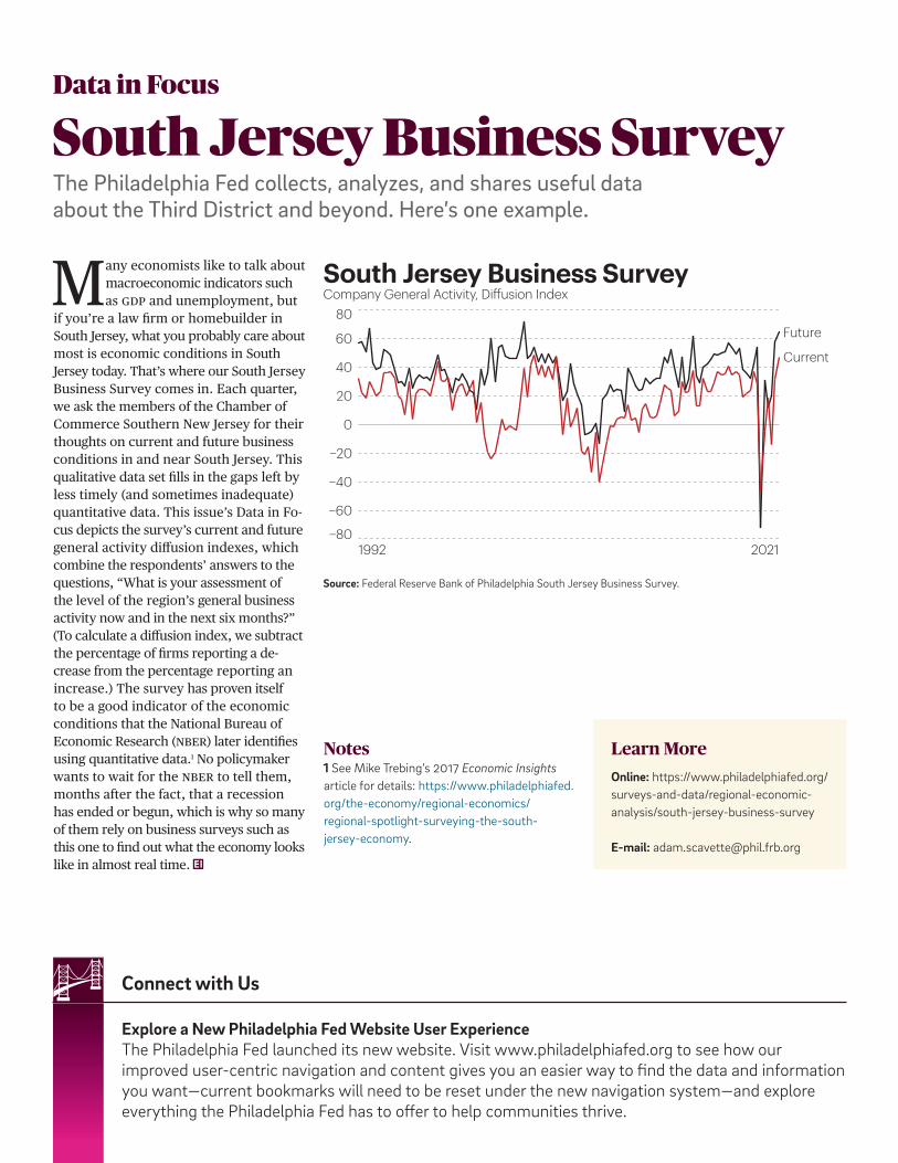
Explore a New Philadelphia Fed Website User ExperienceThe Philadelphia Fed launched its new website. Visit www.philadelphiafed.org to see how our improved user-centric navigation and content gives you an easier way to find the data and information you want—current bookmarks will need to be reset under the new navigation system—and explore everything the Philadelphia Fed has to offer to help communities thrive.

Connect with Us

Many economists like to talk about macroeconomic indicators such as GDP and unemployment, but

if you’re a law firm or homebuilder in South Jersey, what you probably care about most is economic conditions in South Jersey today. That’s where our South Jersey Business Survey comes in. Each quarter, we ask the members of the Chamber of Commerce Southern New Jersey for their thoughts on current and future business conditions in and near South Jersey. This qualitative data set fills in the gaps left by less timely (and sometimes inadequate) quantitative data. This issue’s Data in Fo-cus depicts the survey’s current and future general activity diffusion indexes, which combine the respondents’ answers to the questions, “What is your assessment of the level of the region’s general business activity now and in the next six months?” (To calculate a diffusion index, we subtract the percentage of firms reporting a de-crease from the percentage reporting an increase.) The survey has proven itself to be a good indicator of the economic conditions that the National Bureau of Economic Research (NBER) later identifies using quantitative data.1 No policymaker wants to wait for the NBER to tell them, months after the fact, that a recession has ended or begun, which is why so many of them rely on business surveys such as this one to find out what the economy looks like in almost real time.

Notes1 See Mike Trebing’s 2017 Economic Insights article for details: https://www.philadelphiafed.org/the-economy/regional-economics/ regional-spotlight-surveying-the-south- jersey-economy.

South Jersey Business SurveyCompany General Activity, Diffusion Index

1992 2021−80

−60

−40

−20

0

20

40

60

80Future

Current

Learn MoreOnline: https://www.philadelphiafed.org/ surveys-and-data/regional-economic- analysis/south-jersey-business-survey

E-mail: [email protected]

Source: Federal Reserve Bank of Philadelphia South Jersey Business Survey.

Data in Focus

South Jersey Business SurveyThe Philadelphia Fed collects, analyzes, and shares useful data about the Third District and beyond. Here’s one example.

https://www.philadelphiafed.org/

https://www.philadelphiafed.org/the-economy/regional-economics/regional-spotlight-surveying-the-south-jersey-economy




https://www.philadelphiafed.org/surveys-and-data/regional-economic-analysis/south-jersey-business-survey



mailto:adam.scavette%40phil.frb.org?subject=

ADDRESS SERVICE REQUESTED

PRESORTED STANDARDU.S. POSTAGE

PAID

PHILADELPHIA, PAPERMIT #583

From Philadelphia, Pennsylvania, the birthplace of American finance, comes Economic Insights.

Featuring articles about how Americans work, invest, spend…and so much more.

2016 Q1

2020 Q1

2017 Q2

2020 Q2

2018 Q1

2020 Q3

2019 Q1

2020 Q4

Ten Independence MallPhiladelphia, Pennsylvania 19106-1574

q&a research update

Documents