publications - university of arizonaboguo/pdfs/publications/2014_gu… · · 2017-08-27scenarios...

RESEARCH ARTICLE10.1002/2013WR015215

A vertically integrated model with vertical dynamicsfor CO2 storageBo Guo1, Karl W. Bandilla1, Florian Doster1,2, Eirik Keilegavlen1,2, and Michael A. Celia1

1Department of Civil and Environmental Engineering, Princeton University, Princeton, New Jersey, USA, 2Department ofMathematics, University of Bergen, Bergen, Norway

Abstract Conventional vertically integrated models for CO2 storage usually adopt a vertical equilibrium(VE) assumption, which states that due to strong buoyancy, CO2 and brine segregate quickly, so that the flu-ids can be assumed to have essentially hydrostatic pressure distributions in the vertical direction. However,the VE assumption is inappropriate when the time scale of fluid segregation is not small relative to the simu-lation time. By casting the vertically integrated equations into a multiscale framework, a new vertically inte-grated model can be developed that relaxes the VE assumption, thereby allowing vertical dynamics to bemodeled explicitly. The model maintains much of the computational efficiency of vertical integration whileallowing a much wider range of problems to be modeled. Numerical tests of the new model, using injectionscenarios with typical parameter sets, show excellent behavior of the new approach for homogeneous geo-logic formations.

1. Introduction

Geological sequestration of carbon dioxide (CO2) has been proposed as a promising mitigation strategy toreduce the global warming effects caused by increasing anthropogenic CO2 emissions [Benson et al., 2005].Such technology involves capturing anthropogenic CO2 and injecting the captured carbon into permeablegeologic formations deep in the subsurface. One important type of storage formation is deep saline aqui-fers, where CO2 would be injected into a formation whose pore space is initially filled with brine. In order toeffectively mitigate the global warming problem, geological sequestration of CO2 has to be deployed at avery large scale, with injection increasing to on the order of 3.5 billion tons of carbon per year over the next50 years [Pacala and Socolow, 2004]. With such large amounts of fluids being injected, a range of engineer-ing questions have to be answered to determine if the CO2 will be stored safely over a long period of time.These questions include the spatial extent of the CO2 plume, the spatial extent of significant pressure per-turbations, and the risk of fluid leakage out of the target formation. To address these issues, mathematicalmodels representing the physical processes of the system are required.

Injection of CO2 into a saline aquifer leads to a flow system with multiple fluid phases, which typicallyinvolves an invading less viscous and less dense supercritical CO2 phase and a resident more viscous anddenser brine phase. Mathematical models for the multiphase flow system vary across a broad range of com-plexity, from simplified analytical solutions [Dentz and Tartakovsky, 2009; Hesse et al., 2008, 2007; Huppertand Woods, 1995; Juanes et al., 2010; Lyle et al., 2005; Nordbotten and Celia, 2006; Nordbotten et al., 2005;Vella and Huppert, 2006; Woods and Mason, 2000] to full three-dimensional multiphase multicomponentmodels, such as ECLIPSE [Schlumberger, 2010], TOUGH2 [Pruess, 2005], STOMP [White and Oostrom, 1997],and FEHM [Zyvoloski et al., 1997]. One family of simplified models has been developed based on theassumption of vertical equilibrium (VE) [Dentz and Tartakovsky, 2009; Gasda et al., 2009, 2011, 2012b; Hesseet al., 2008, 2007; Huppert and Woods, 1995; Juanes et al., 2010; Lyle et al., 2005; Nordbotten and Celia, 2006;Nordbotten et al., 2005; Nordbotten and Celia, 2012; Vella and Huppert, 2006; Woods and Mason, 2000]. TheVE assumption states that brine and CO2 segregate instantaneously and are therefore at equilibrium in thevertical direction (i.e., the pressure distribution for each fluid is essentially hydrostatic). This assumptionimplies that the functional form of the phase pressures in the vertical direction is known, a priori. Therefore,the solution in the vertical does not need to be computed, so that the governing equations for the systemare integrated across the vertical direction, resulting in a set of equations defined in the horizontal plane.

Key Points:� A vertically integrated model with

vertical dynamics is developed� It extends the applicability of

vertically integrated models for CO2

storage� It maintains most computational

advantages of vertical equilibriummodels

Correspondence to:B. Guo,[email protected]

Citation:Guo, B., K. W. Bandilla, F. Doster, E.Keilegavlen, and M. A. Celia (2014), Avertically integrated model withvertical dynamics for CO2 storage,Water Resour. Res., 50, doi:10.1002/2013WR015215.

Received 23 DEC 2013

Accepted 4 JUL 2014

Accepted article online 10 JUL 2014

GUO ET AL. VC 2014. American Geophysical Union. All Rights Reserved. 1

Water Resources Research

PUBLICATIONS

http://dx.doi.org/10.1002/2013WR015215

http://onlinelibrary.wiley.com/journal/10.1002/(ISSN)1944-7973/

http://publications.agu.org/

The reduction of spatial dimensionsgives significant computational advan-tages over full three-dimensional mod-els. Such VE models are applicablewhenever the VE assumption is satis-fied. These kinds of models have beenused to study many problems relatedto geological storage of CO2 [Bandillaet al., 2012; Court et al., 2012; Gasdaet al., 2009, 2011, 2012a; Nilsen et al.,2011]. However, there are a number ofcases (see, for example, [Court et al.2012]) for which the VE assumption isinappropriate. For example, for targetformations with relatively low verticalpermeability, large formation thickness

or small density contrast between CO2 and brine, the two fluid phases may not reach vertical equilibriumfor a long period of time. For problems where the VE assumption is not appropriate, vertical dynamics ofCO2 and brine flow should be included in the models. At present, this means use of full three-dimensionalmodels for the multiphase system.

Here we propose a new model that maintains the computational efficiencies of a vertically integratedmodel while relaxing the assumption of vertical equilibrium. We cast the new model in a multiscale frame-work, in direct analogy to the recent presentations of VE models (see, for example, Nordbotten and Celia[2012]). The coarse scale is the horizontal domain while the fine scale is the vertical domain, which corre-sponds to the thickness of the formation. Because the formation thickness is usually much smaller than thehorizontal extent, scale separation is appropriate. As in VE models, a vertically integrated equation is solvedfor the pressure defined at the coarse scale. However, in contrast to VE models that solve a second verticallyintegrated equation for the vertically integrated phase saturation, followed by analytical reconstruction ofthe pressure profiles in the vertical direction, the new algorithm solves locally one-dimensional (vertical)dynamic equations to calculate the vertical transients of the fluid saturation profiles. In these locally one-dimensional equations, fine-scale horizontal fluxes are included as sources and sinks. These fine-scale hori-zontal fluxes are computed from the reconstructed vertical fine-scale pressure field. The pressure recon-struction is based on the coarse-scale pressure and the vertical structure of the fine-scale pressure fieldfrom the previous time step. After computing the vertical (fine-sale) saturation, an updated fine-scale pres-sure is reconstructed. The end result is an algorithm that maintains the computational efficiency of a verti-cally integrated pressure equation while capturing the vertical dynamics of the two-phase flow system.

In this paper, we provide details and initial computational results for the new algorithm. We first give a briefoverview of the basic two-phase flow equations for the CO2 storage system. This is followed by a briefreview of VE models. We then give a presentation of the new multiscale algorithm that incorporates the ver-tical dynamics into the vertically integrated framework. Next, we compare the new multiscale model with afull multidimensional model and a VE model to demonstrate its applicability under different conditions.Finally, we summarize the key findings and discuss future extensions and directions.

2. Background

The system of CO2 storage involves a multiphase flow system, which requires a set of equations to repre-sent the flow dynamics of each phase. In this section, we will first introduce the basic equations for the mul-tiphase flow system and then review the VE models that approximate the system as two dimensional byassuming hydrostatic pressure profiles for both phases.

2.1. Two-Phase Flow EquationsInjection of CO2 into deep saline aquifers usually leads to a two-phase flow system with the fluids beingbrine and a CO2-rich phase. Figure 1 depicts the flow dynamics of injected CO2 and resident brine, both ofwhich have significant horizontal velocities because of the imposed pressure gradient. In addition, the

!!

CO2CO2

Brine Brine

Qwell

CO2 Brine

z

r

Figure 1. A schematic description of CO2 injection in an aquifer in the r-z crosssection, where a vertical CO2 injection well is placed on the left side (r 5 0) and avertical column is highlighted to demonstrate flow dynamics of CO2 and brine.The arrows represent flow directions of the two fluid phases.

Water Resources Research 10.1002/2013WR015215


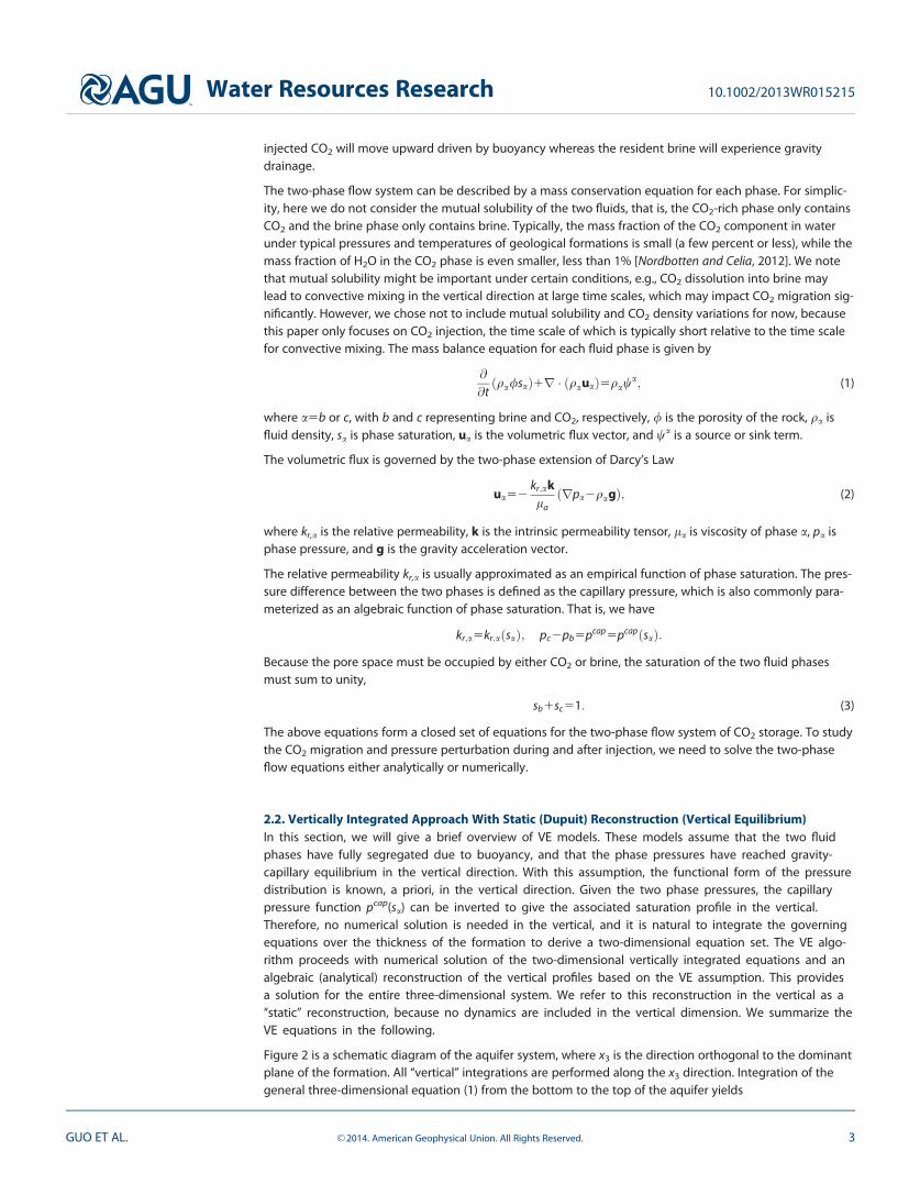
injected CO2 will move upward driven by buoyancy whereas the resident brine will experience gravitydrainage.

The two-phase flow system can be described by a mass conservation equation for each phase. For simplic-ity, here we do not consider the mutual solubility of the two fluids, that is, the CO2-rich phase only containsCO2 and the brine phase only contains brine. Typically, the mass fraction of the CO2 component in waterunder typical pressures and temperatures of geological formations is small (a few percent or less), while themass fraction of H2O in the CO2 phase is even smaller, less than 1% [Nordbotten and Celia, 2012]. We notethat mutual solubility might be important under certain conditions, e.g., CO2 dissolution into brine maylead to convective mixing in the vertical direction at large time scales, which may impact CO2 migration sig-nificantly. However, we chose not to include mutual solubility and CO2 density variations for now, becausethis paper only focuses on CO2 injection, the time scale of which is typically short relative to the time scalefor convective mixing. The mass balance equation for each fluid phase is given by

@

@tqa/sað Þ1r � qauað Þ5qaw

a; (1)

where a5b or c, with b and c representing brine and CO2, respectively, / is the porosity of the rock, qa isfluid density, sa is phase saturation, ua is the volumetric flux vector, and wa is a source or sink term.

The volumetric flux is governed by the two-phase extension of Darcy’s Law

ua52kr;aklaðrpa2qagÞ; (2)

where kr,a is the relative permeability, k is the intrinsic permeability tensor, la is viscosity of phase a, pa isphase pressure, and g is the gravity acceleration vector.

The relative permeability kr,a is usually approximated as an empirical function of phase saturation. The pres-sure difference between the two phases is defined as the capillary pressure, which is also commonly para-meterized as an algebraic function of phase saturation. That is, we have

kr;a5kr;aðsaÞ; pc2pb5pcap5pcapðsaÞ:

Because the pore space must be occupied by either CO2 or brine, the saturation of the two fluid phasesmust sum to unity,

sb1sc51: (3)

The above equations form a closed set of equations for the two-phase flow system of CO2 storage. To studythe CO2 migration and pressure perturbation during and after injection, we need to solve the two-phaseflow equations either analytically or numerically.

2.2. Vertically Integrated Approach With Static (Dupuit) Reconstruction (Vertical Equilibrium)In this section, we will give a brief overview of VE models. These models assume that the two fluidphases have fully segregated due to buoyancy, and that the phase pressures have reached gravity-capillary equilibrium in the vertical direction. With this assumption, the functional form of the pressuredistribution is known, a priori, in the vertical direction. Given the two phase pressures, the capillarypressure function pcap(sa) can be inverted to give the associated saturation profile in the vertical.Therefore, no numerical solution is needed in the vertical, and it is natural to integrate the governingequations over the thickness of the formation to derive a two-dimensional equation set. The VE algo-rithm proceeds with numerical solution of the two-dimensional vertically integrated equations and analgebraic (analytical) reconstruction of the vertical profiles based on the VE assumption. This providesa solution for the entire three-dimensional system. We refer to this reconstruction in the vertical as a‘‘static’’ reconstruction, because no dynamics are included in the vertical dimension. We summarize theVE equations in the following.

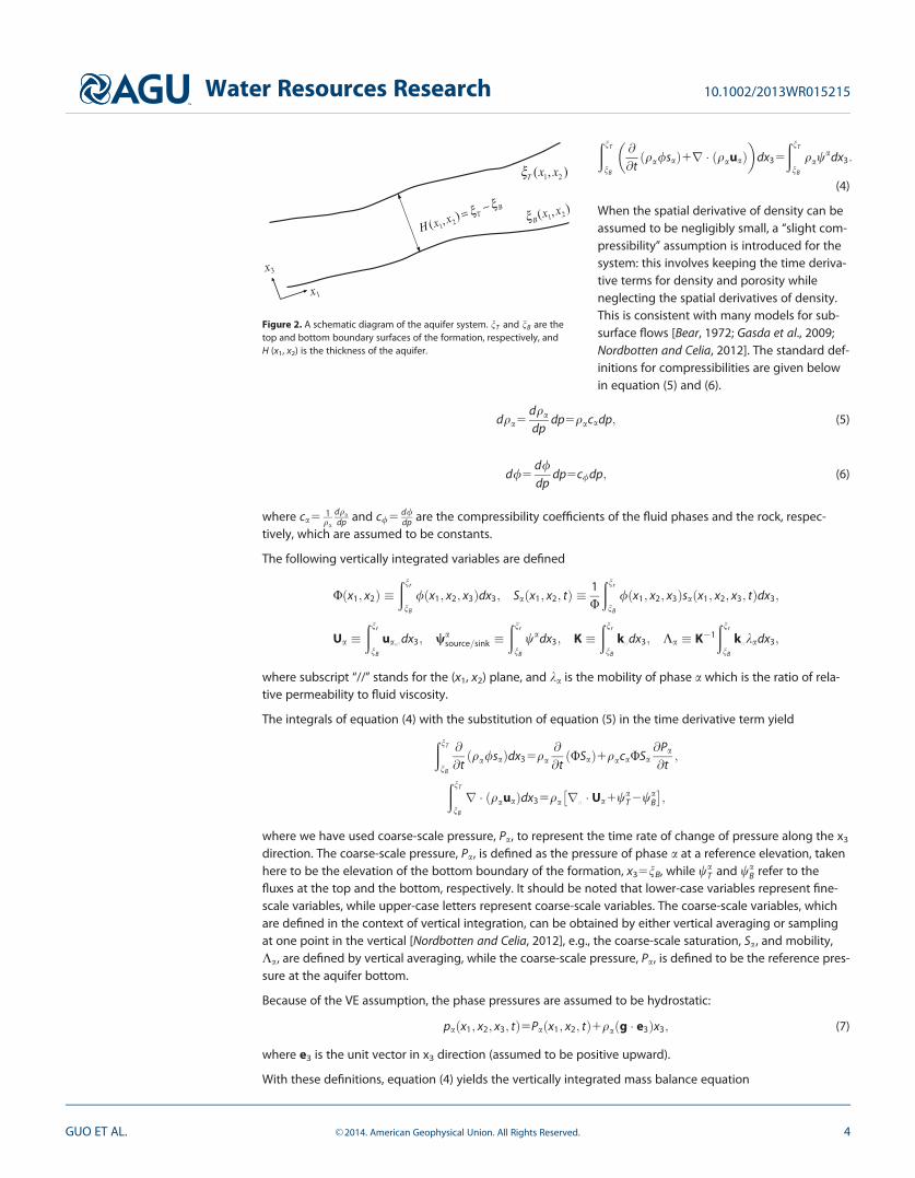
Figure 2 is a schematic diagram of the aquifer system, where x3 is the direction orthogonal to the dominantplane of the formation. All ‘‘vertical’’ integrations are performed along the x3 direction. Integration of thegeneral three-dimensional equation (1) from the bottom to the top of the aquifer yields



ðnT

nB

@

@tqa/sað Þ1r � qauað Þ

� �dx35

ðnT

nB

qawadx3:

(4)

When the spatial derivative of density can beassumed to be negligibly small, a ‘‘slight com-pressibility’’ assumption is introduced for thesystem: this involves keeping the time deriva-tive terms for density and porosity whileneglecting the spatial derivatives of density.This is consistent with many models for sub-surface flows [Bear, 1972; Gasda et al., 2009;Nordbotten and Celia, 2012]. The standard def-initions for compressibilities are given belowin equation (5) and (6).

dqa5dqa

dpdp5qacadp; (5)

d/5d/dp

dp5c/dp; (6)

where ca51qa

dqadp and c/5 d/

dp are the compressibility coefficients of the fluid phases and the rock, respec-tively, which are assumed to be constants.

The following vertically integrated variables are defined

Uðx1; x2Þ �ðnr

nB

/ðx1; x2; x3Þdx3; Saðx1; x2; tÞ � 1U

ðnr

nB

/ðx1; x2; x3Þsaðx1; x2; x3; tÞdx3;

Ua �ðnr

nB

ua;==dx3; wasource=sink �

ðnr

nB

wadx3; K �ðnr

nB

k==dx3; Ka � K21

ðnr

nB

k==kadx3;

where subscript ‘‘//’’ stands for the (x1, x2) plane, and ka is the mobility of phase a which is the ratio of rela-tive permeability to fluid viscosity.

The integrals of equation (4) with the substitution of equation (5) in the time derivative term yield

ðnT

nB

@

@tqa/sað Þdx35qa

@

@tðUSaÞ1qacaUSa

@Pa

@t;

ðnT

nB

r � qauað Þdx35qa r==� Ua1wa

T 2waB

� �;

where we have used coarse-scale pressure, Pa, to represent the time rate of change of pressure along the x3

direction. The coarse-scale pressure, Pa, is defined as the pressure of phase a at a reference elevation, takenhere to be the elevation of the bottom boundary of the formation, x35nB, while wa

T and waB refer to the

fluxes at the top and the bottom, respectively. It should be noted that lower-case variables represent fine-scale variables, while upper-case letters represent coarse-scale variables. The coarse-scale variables, whichare defined in the context of vertical integration, can be obtained by either vertical averaging or samplingat one point in the vertical [Nordbotten and Celia, 2012], e.g., the coarse-scale saturation, Sa, and mobility,Ka, are defined by vertical averaging, while the coarse-scale pressure, Pa, is defined to be the reference pres-sure at the aquifer bottom.

Because of the VE assumption, the phase pressures are assumed to be hydrostatic:

paðx1; x2; x3; tÞ5Paðx1; x2; tÞ1qaðg � e3Þx3; (7)

where e3 is the unit vector in x3 direction (assumed to be positive upward).

With these definitions, equation (4) yields the vertically integrated mass balance equation

B(x1, x2)

H (x1, x 2) = TB

x3

T (x1, x2 )

x1

Figure 2. A schematic diagram of the aquifer system. nT and nB are thetop and bottom boundary surfaces of the formation, respectively, andH (x1, x2) is the thickness of the aquifer.



@ USað Þ@t

1caUSa@Pa

@t1r � Ua5Wa

source=sink2waT 1wa

B5Wa: (8)

The integrated flux in equation (8) is

Ua52KKa � ðr==Pa2qaGÞ; (9)

where G5e==� g1ðg � e3Þr==

nB and e==5ðe1; e2ÞT .

Based on kr,a(sa) and pcap(sa), the vertically integrated mobility and capillary pressure can also be related tothe vertically integrated saturation algebraically, such that Ka5KaðSaÞ, P̂c2Pb5PcapðSaÞ. The coarse-scalecapillary pressure, Pcap, is a ‘‘pseudocapillary pressure,’’ which is defined as the difference between thecoarse-scale pressures. Those pressures are, by definition, the phase pressures evaluated at the bottom ofthe formation; we use the notation P̂c to denote the hydrostatic extension of the CO2 phase pressure eval-uated at the bottom of the formation, given that for many locations the CO2 phase will not be present atthe bottom boundary (fB). When neglecting capillary pressure, the functions Ka(Sa) and Pcap(Sa) are linearand simple to derive. A detailed derivation of these two functions can be found in [Nordbotten and Celia,2012]. Although these functions become nonlinear when capillary pressure is included, they can be derivedin an analogous way.

The vertically integrated phase saturations also sum to unity.

Sc1Sb51 (10)

By solving the vertically integrated two-dimensional equations, we can compute the vertically integratedsaturation and one of the bottom phase pressures, both of which are coarse-scale variables. The pressureand saturation profiles along the vertical direction, which represent the fine scale of the problem, can thenbe reconstructed algebraically based on the VE assumption.

The applicability of VE models depends on the time scale of fluid segregation (ts) compared to the simula-tion time T. If the segregation time is small relative to T, then vertical equilibrium is usually a good approxi-mation; otherwise the VE assumption is not applicable. The segregation time scale can be estimated from

ts �H/lb

kr;b;finekzDqg; (11)

where H is formation thickness, lb is brine viscosity, kr;b;fine is the fine-scale relative permeability of brine, kz

is vertical permeability of the formation, Dq is the density difference between CO2 and brine, g is the magni-tude of gravity acceleration.

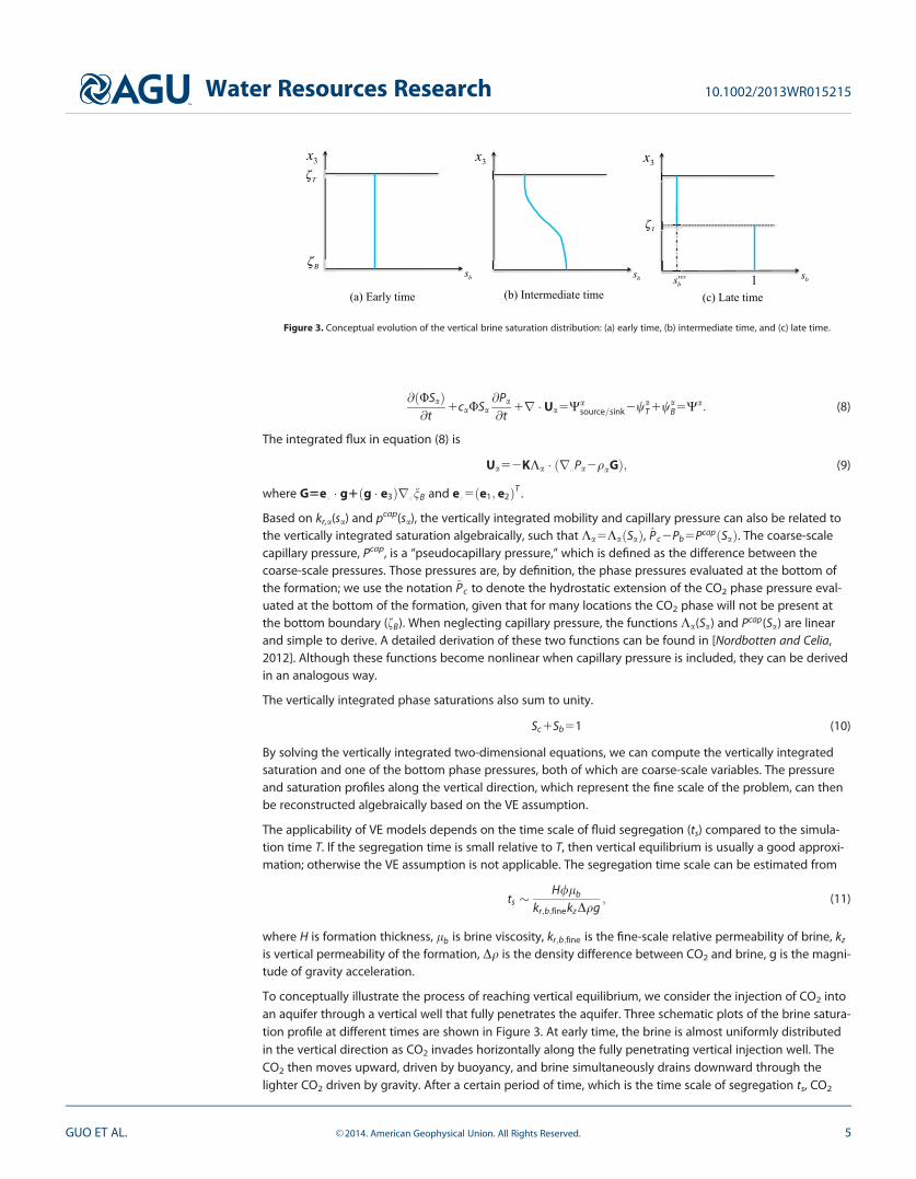
To conceptually illustrate the process of reaching vertical equilibrium, we consider the injection of CO2 intoan aquifer through a vertical well that fully penetrates the aquifer. Three schematic plots of the brine satura-tion profile at different times are shown in Figure 3. At early time, the brine is almost uniformly distributedin the vertical direction as CO2 invades horizontally along the fully penetrating vertical injection well. TheCO2 then moves upward, driven by buoyancy, and brine simultaneously drains downward through thelighter CO2 driven by gravity. After a certain period of time, which is the time scale of segregation ts, CO2

sb1sbres

I

x3

sb

x3

sb

T

B

x3

(a) Early time (b) Intermediate time (c) Late time

Figure 3. Conceptual evolution of the vertical brine saturation distribution: (a) early time, (b) intermediate time, and (c) late time.



and brine segregate essentiallycompletely with CO2 residing ontop of brine. For simplicity, in Figure3, we have neglected local capillarypressure; therefore, when both CO2

and brine reach vertical equilibrium,they form a macroscopic sharpinterface, fI , as shown in Figure 3c. Ifts� T, then we can usually neglectthe vertical redistribution processand simply assume CO2 and brinehave already segregated; this is the

VE assumption. However, when ts is comparable or even larger than T, we have to include the verticaldynamics of CO2 and brine in order to accurately predict CO2 migration.

3. Multiscale Algorithm—Vertical Dynamic Reconstruction

The VE model is accurate and computationally efficient as long as the VE assumption is satisfied. However,such a simplified model will not be applicable when the time scale of fluid segregation is not small relativeto the simulation time. In order to extend the applicability of vertically integrated models, we present a mul-tiscale method that relaxes the VE assumption and includes the vertical dynamics of CO2 and brine, but stilluses the vertically integrated framework. We refer to this multiscale method as ‘‘dynamic reconstruction,’’ asopposed to static reconstruction in the VE model, because in the new approach flow dynamics are includedin the vertical reconstruction. In this section, we first describe the dynamic reconstruction algorithm andthen derive the equations for both the coarse and fine scales. We then present the numerical solution pro-cedure that we have implemented.

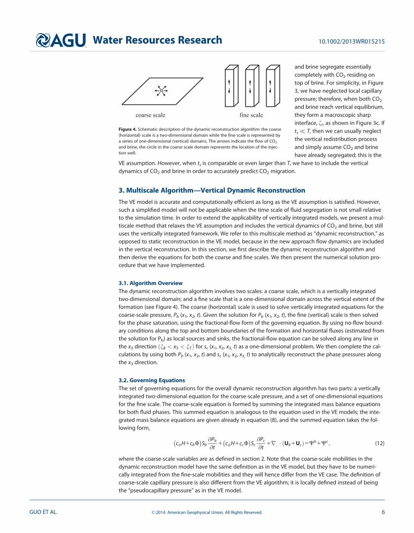
3.1. Algorithm OverviewThe dynamic reconstruction algorithm involves two scales: a coarse scale, which is a vertically integratedtwo-dimensional domain; and a fine scale that is a one-dimensional domain across the vertical extent of theformation (see Figure 4). The coarse (horizontal) scale is used to solve vertically integrated equations for thecoarse-scale pressure, Pb (x1, x2, t). Given the solution for Pb (x1, x2, t), the fine (vertical) scale is then solvedfor the phase saturation, using the fractional-flow form of the governing equation. By using no-flow bound-ary conditions along the top and bottom boundaries of the formation and horizontal fluxes (estimated fromthe solution for Pb) as local sources and sinks, the fractional-flow equation can be solved along any line inthe x3 direction ðnB < x3 < nT Þ for sc (x1, x2, x3, t) as a one-dimensional problem. We then complete the cal-culations by using both Pb (x1, x2, t) and sc (x1, x2, x3, t) to analytically reconstruct the phase pressures alongthe x3 direction.

3.2. Governing EquationsThe set of governing equations for the overall dynamic reconstruction algorithm has two parts: a verticallyintegrated two-dimensional equation for the coarse-scale pressure, and a set of one-dimensional equationsfor the fine scale. The coarse-scale equation is formed by summing the integrated mass balance equationsfor both fluid phases. This summed equation is analogous to the equation used in the VE models; the inte-grated mass balance equations are given already in equation (8), and the summed equation takes the fol-lowing form,

c/H1cbU� �

Sb@Pb

@t1 c/H1ccU� �

Sc@Pc

@t1r

==� Ub1Ucð Þ5Wb1Wc; (12)

where the coarse-scale variables are as defined in section 2. Note that the coarse-scale mobilities in thedynamic reconstruction model have the same definition as in the VE model, but they have to be numeri-cally integrated from the fine-scale mobilities and they will hence differ from the VE case. The definition ofcoarse-scale capillary pressure is also different from the VE algorithm; it is locally defined instead of beingthe ‘‘pseudocapillary pressure’’ as in the VE model.

coarse scale fine scale

Figure 4. Schematic description of the dynamic reconstruction algorithm: the coarse(horizontal) scale is a two-dimensional domain while the fine scale is represented bya series of one-dimensional (vertical) domains. The arrows indicate the flow of CO2

and brine, the circle in the coarse scale domain represents the location of the injec-tion well.



To this point, the procedure is almost identical to the vertical equilibrium approach, the differences being inthe details of the coarse-scale coefficients as described above. However, as shown in equation (7), the VEapproach imposes a strict hydrostatic condition on both phase pressures, which serves to define the pres-sure structure used in the definition of integrated fluxes Ub and Uc . The VE pressure distribution is inappro-priate in the new algorithm, except in the limits where VE is applicable. Therefore, in the dynamicreconstruction, we use a more general pressure reconstruction. In the spirit of equation (7), we write a gen-eralized pressure function as

paðx1; x2; x3; tÞ5Paðx1; x2; tÞ1paðx1; x2; x3; tÞ: (13)

In this equation, the function pa defines the vertical fine-scale reconstruction of the pressure field for phasea. Specific choices for this reconstruction function are discussed later in this section. With this reconstructedpressure, the integrated fluxes can be calculated by computing the gradient in the x1 and x2 directions ofthe function pa. Equation (12) can then be solved for a coarse-scale pressure, which can be chosen as eitherPb or Pc or any combination of these two pressures. Pb is chosen in this paper. Details of the numerical solu-tion algorithm are given in section 3.3.

In the fine-scale model, the phase mass balance equations are rearranged to focus on the vertical dynamics.The fine-scale mass balance for each phase can be written as follows,

@ qa/sað Þ@t

1@ðqaua;3Þ@x3

5qawa2r

==� qaua;==� �

; (14)

where ua,3 is the flux of fluid phase a in the x3 direction, and ua;== is the flux in the (x1, x2) plane which will beestimated from the solution of equations (12) and (13) by using equation (15),

ua;==52k==ka � r==

pa2qa e==� gð Þ½ �: (15)

Again as in the vertical equilibrium case, we assume ‘‘slight compressibility,’’ leading to

/@sa

@t1 c/1/ca� �

sa@pa

@t1@ua;3

@x35wa2r

==� ua;==: (16)

Equation (16) is summed over the two phases, and the resulting equation is used to estimate the total flux,uTOT,3 in the x3 direction, where uTOT,35ub,31uc,3. Given the total flux values in the x3 direction, the vertical phaseflux ua,3 can be calculated using the fractional-flow form of Darcy’s Law, which takes the following form,

ub;35fb � uTOT;32k3kcDqg1kck3@pcap

@x3

� �

uc;35fc � uTOT;31k3kbDqg2kbk3@pcap

@x3

� �;

(17)

where k3 is permeability in x3 direction, and fa is the fractional-flow function, given by

fa5ka

kb1kb:

At this point, all the vertical and horizontal phase fluxes are known, allowing us to compute (reconstruct)the phase saturations using equation (16).

Finally, we return to the issue of pressure reconstruction on the fine scale (equation (13)). We seek a pres-sure reconstruction function that is simple to compute, is physically motivated, and produces the VE modelat the appropriate limits. After experimenting with a number of choices, our current preferred choice is thefollowing saturation-weighted pressure functions for the two phases:

@pc

@x352ðscqc1sbqbÞg1sb

@pcapðsbÞ@x3

@pb

@x352ðscqc1sbqbÞg2sc

@pcapðsbÞ@x3

:

(18)

From equation (18), the function pa in equation (13) can be derived. For example, when a5b, integrationfrom the bottom of the formation yields



pbðx1; x2; x3; tÞ5Pbðx1; x2; tÞ2ðx3

nB

ðscqc1sbqbÞg1sc@pcapðsbÞ@x3

� dx3: (19)

It should be noted that the reconstructed fine-scale pressure is only used to compute horizontal fine-scalefluxes, and is not directly used in the vertical flux calculation. Thus, the appropriateness of the pressurereconstruction only depends on how well it captures the horizontal fine-scale fluxes. There are three forcesthat drive the horizontal flow: the viscous force, capillary pressure, and buoyancy. Different forces becomedominant in different regimes or periods. For the regime that is close to the injection well or before CO2

and brine segregate, viscous forces dominate. For the regime that is far from the injection well, or after CO2

and brine segregate, capillary pressure and gravity forces become dominant. The pressure reconstructionshould be able to capture the evolution of the dominant forces. Any reconstruction that has the coarse-scale pressure included can approximately capture the viscous forces when viscous forces are dominant,while the saturation-weighted hydrostatic pressure profile is currently the only reconstruction we havedeveloped that not only accounts for the viscous forces, but also captures the capillary pressure and buoy-ancy when these two forces become dominant. Other options could be chosen, for example, instead ofusing the fine-scale reconstructed pressure field, the coarse-scale horizontal pressure gradient can be usedto compute the fine-scale fluxes (that is, apply the coarse pressure gradient along the entire vertical). Thisoption gives good results when CO2 and brine are not segregated, meaning it captures the viscous forceswell, but it induces significant errors when CO2 and brine segregate and reach vertical equilibrium in somecases. This is simply because when CO2 and brine are in equilibrium, fine-scale pressure gradient is differentfrom the coarse-scale pressure gradient and that difference is largely due to capillary pressure and buoyantforce. Other choices may be explored for the pressure reconstruction, but our results to date indicate thatthe saturation-weighted reconstruction gives good results.

3.3. Numerical Solution ProcedureTo solve the dynamic reconstruction model numerically we discretize space by using a standard cell-centered finite-volume method. For the time discretization, we use a scheme analogous to the implicit pres-sure and explicit saturation (IMPES) method: an implicit treatment of the pressure at the coarse scale andan explicit treatment of saturation at the fine-scale decouples the two scales. Hence, we are able to firstsolve the coarse-scale pressure implicitly and then calculate the fine-scale saturations explicitly. Details ofthe algorithm implementation are presented in this section. For the sake of clarity, we use continuous oper-ators in space in our exposition.

The time-discrete version of equation (12) with implicit brine pressure Pb and explicit treatment of satura-tions is given by

c/H1cbUSbn1ccUSc

n� � Pb

n112Pbn

Dt1 c/H1ccU� �

Scn Pcap;n2Pcap;n21

Dt

2r==� K ðKb

n1KcnÞ � r

==Pb

n111Kcnr

==Pcap;n2 Kb

nqb1Kcnqcð Þðe== � gÞ½ �1

ðnT

nB

k==

knbr==

pnb1kn

cr==pn

c

� �dx3

�:

5Wb;n111Wc;n11:

(20)

where superscript n stands for the discrete time level tn and n11 stands for tn11. This is a linear equationfor the coarse-scale pressure Pn11

b at time tn11 that can be solved by a sparse matrix solver.

For the fine-scale transport of the saturations using equation (16), we first calculate the horizontal phasefluxes as follows

un11;�a;== 52k

==kn

a � r==pn11;�

a 2qa e==� gð Þ

� �: (21)

where pn11;�a ðx1; x2; x3Þ5Pn11

a ðx1; x2Þ1pnaðx1; x2; x3Þ, and the superscript * denotes that the variable is an

approximation at time tn11.

The horizontal total flux un11;�TOT;== 5un11;�

b;== 1un11;�c;== is then used to calculate the vertical total flux from the time-

discrete version of equation (16) summed over the two phases, that is

@un11;�TOT;3

@x352r

==� un11;�

TOT;== 1wb;n111wc;n112 c/1/cb� �

sbpn11;�

b 2pnb

Dt2 c/1/cc� �

scpn11;�

c 2pnc

Dt: (22)



With the vertical total flux un11;�TOT;3 and no-flow boundary conditions at the top and bottom of the formation,

we obtain the phase fluxes with the time-discrete version of equation (17) given by

un11;�b;3 5f n

b � un11;�TOT;3 2k3k

nc Dqg1kn

c k3@pcap;n

@x3

� �

un11;�c;3 5f n

c � un11;�TOT;3 1k3k

nbDqg2kn

bk3@pcap;n

@x3

� �:

(23)

Then the saturations sn11a can be computed explicitly using the time-discrete version of equation (16) that

reads as

/sn11a 2sn

a

Dt1 c/1/ca� �

sapn11;�

a 2pna

Dt1@un11;�

a;3

@x35wa;n112r

==� un11;�

a;== : (24)

Finally, we obtain the updated pressure field in the vertical direction as

pn11b 5Pn11

b 2

ðx3

nB

ðsn11c qc1sn11

b qbÞg1sn11c

@pcap sn11b

� �@x3

� dx3

pn11c 5Pn11

b 1Pcap;n112

ðx3

nB

ðsn11c qc1sn11

b qbÞg2sn11b

@pcap sn11b

� �@x3

� dx3

(25)

The solution procedure is summarized in table 1.

4. Results

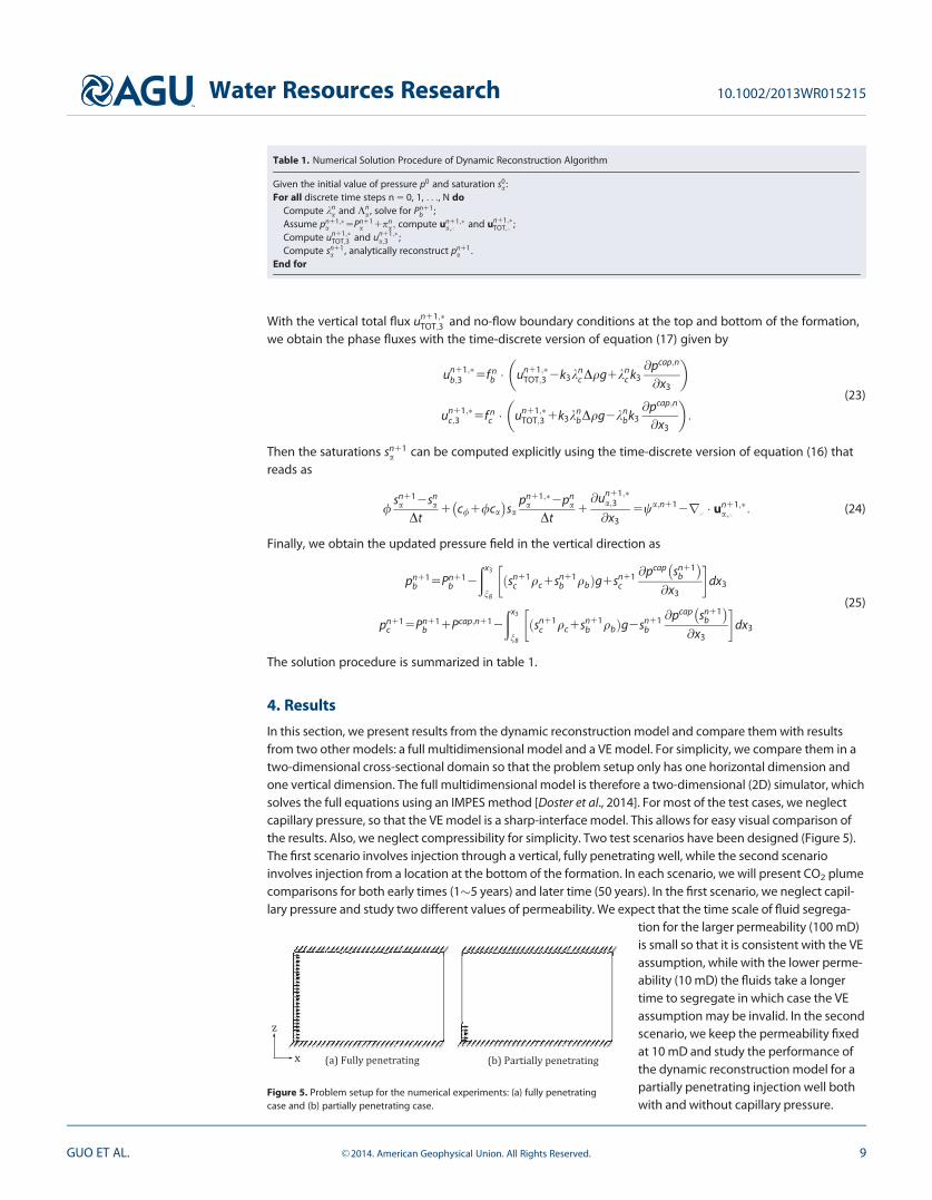
In this section, we present results from the dynamic reconstruction model and compare them with resultsfrom two other models: a full multidimensional model and a VE model. For simplicity, we compare them in atwo-dimensional cross-sectional domain so that the problem setup only has one horizontal dimension andone vertical dimension. The full multidimensional model is therefore a two-dimensional (2D) simulator, whichsolves the full equations using an IMPES method [Doster et al., 2014]. For most of the test cases, we neglectcapillary pressure, so that the VE model is a sharp-interface model. This allows for easy visual comparison ofthe results. Also, we neglect compressibility for simplicity. Two test scenarios have been designed (Figure 5).The first scenario involves injection through a vertical, fully penetrating well, while the second scenarioinvolves injection from a location at the bottom of the formation. In each scenario, we will present CO2 plumecomparisons for both early times (1�5 years) and later time (50 years). In the first scenario, we neglect capil-lary pressure and study two different values of permeability. We expect that the time scale of fluid segrega-

tion for the larger permeability (100 mD)is small so that it is consistent with the VEassumption, while with the lower perme-ability (10 mD) the fluids take a longertime to segregate in which case the VEassumption may be invalid. In the secondscenario, we keep the permeability fixedat 10 mD and study the performance ofthe dynamic reconstruction model for apartially penetrating injection well bothwith and without capillary pressure.

Figure 5. Problem setup for the numerical experiments: (a) fully penetratingcase and (b) partially penetrating case.

Table 1. Numerical Solution Procedure of Dynamic Reconstruction Algorithm

Given the initial value of pressure p0 and saturation s0a :

For all discrete time steps n 5 0, 1, . . ., N doCompute kn

a and Kna , solve for Pn11

b ;Assume pn11;�

a 5Pn11a 1pn

a ; compute un11;�a;== and un11;�

TOT;== ;Compute un11;�

TOT;3 and un11;�a;3 ;

Compute sn11a , analytically reconstruct pn11

a .End for



The problem setup for both scenarios is shown in Figure 5. Top and bottom boundaries are no-flow. Alongthe left boundary, CO2 is injected from a well at a constant flow rate. The well spans the entire thicknessof the formation in the fully penetrating case, and only the bottom 1 m in the partially penetrating case. Alongthe right boundary, a flux boundary condition is imposed where we extract, uniformly along the vertical direc-tion, the same mass of fluid as we inject on the left side. The formation is 50 m thick, and the domain size inthe x direction depends on different simulation times: a shorter length is chosen for early time simulations toallow use of fine grid spacing. For early time simulations, the domain size is lx 5 1500 m, lz 5 50 m, and thegrid size is Dx 5 5 m, Dz 5 0.2 m; for later time, the domain size is lx 5 15,000 m, lz 5 50 m, and the grid size isDx 5 25 m, Dz 5 0.25 m. We inject 0.71 kg/s/m (2.24 3 1024 Mt/yr/m) CO2 uniformly from the left side, whichis equivalent to a 500 m long horizontal well with an injection rate of about 0.2 Mt CO2 per year. Densities ofCO2 and brine are 710 and 1000 kg/m3; viscosities are 4.25 3 1025 and 3.0 3 1024 Pa s, respectively; porosityof the rock formation is 0.15. We use Brooks-Corey curves for relative permeability and capillary pressure (whencapillary pressure is included) with pore size distribution index as 2.0 and entry pressure as 1.0 3 104 Pa.

4.1. CO2 Plume Comparison for a Fully Penetrating Injection WellIn this section, two cases with fully penetrating injection wells will be presented. The first case involves aformation with relatively low permeability of 10 mD, while the second case has a higher permeability of 100mD. The time scale of vertical fluid segregation is larger in the low-permeability case than in the high-permeability case, so that the low-permeability case is less favorable for VE models.

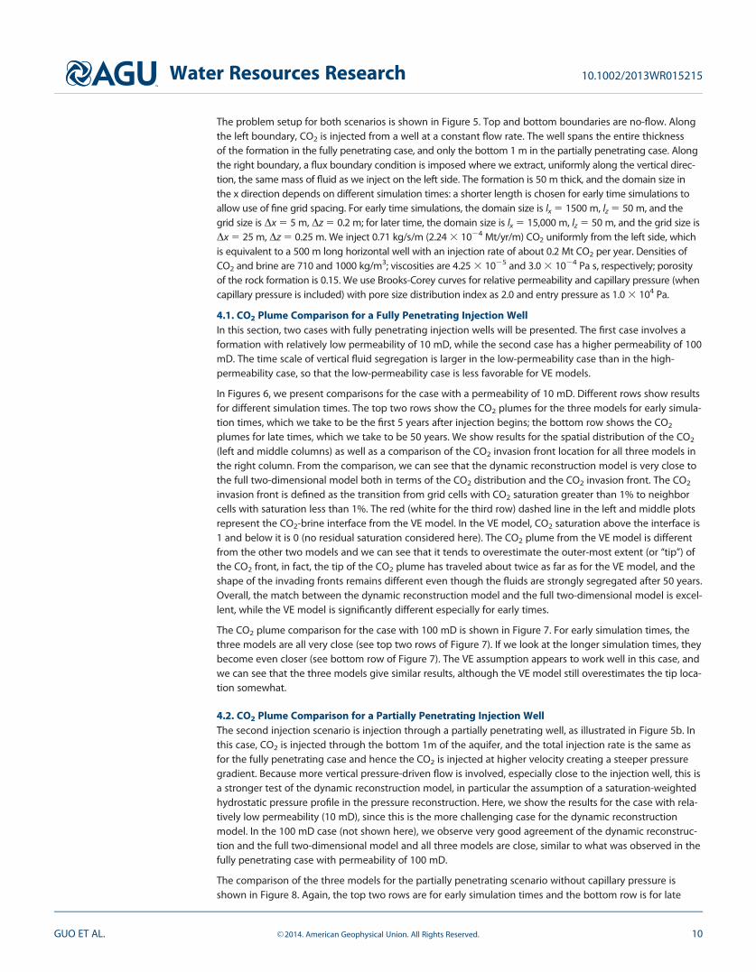
In Figures 6, we present comparisons for the case with a permeability of 10 mD. Different rows show resultsfor different simulation times. The top two rows show the CO2 plumes for the three models for early simula-tion times, which we take to be the first 5 years after injection begins; the bottom row shows the CO2

plumes for late times, which we take to be 50 years. We show results for the spatial distribution of the CO2

(left and middle columns) as well as a comparison of the CO2 invasion front location for all three models inthe right column. From the comparison, we can see that the dynamic reconstruction model is very close tothe full two-dimensional model both in terms of the CO2 distribution and the CO2 invasion front. The CO2

invasion front is defined as the transition from grid cells with CO2 saturation greater than 1% to neighborcells with saturation less than 1%. The red (white for the third row) dashed line in the left and middle plotsrepresent the CO2-brine interface from the VE model. In the VE model, CO2 saturation above the interface is1 and below it is 0 (no residual saturation considered here). The CO2 plume from the VE model is differentfrom the other two models and we can see that it tends to overestimate the outer-most extent (or ‘‘tip’’) ofthe CO2 front, in fact, the tip of the CO2 plume has traveled about twice as far as for the VE model, and theshape of the invading fronts remains different even though the fluids are strongly segregated after 50 years.Overall, the match between the dynamic reconstruction model and the full two-dimensional model is excel-lent, while the VE model is significantly different especially for early times.

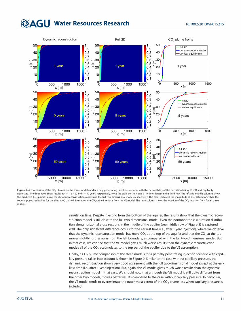
The CO2 plume comparison for the case with 100 mD is shown in Figure 7. For early simulation times, thethree models are all very close (see top two rows of Figure 7). If we look at the longer simulation times, theybecome even closer (see bottom row of Figure 7). The VE assumption appears to work well in this case, andwe can see that the three models give similar results, although the VE model still overestimates the tip loca-tion somewhat.

4.2. CO2 Plume Comparison for a Partially Penetrating Injection WellThe second injection scenario is injection through a partially penetrating well, as illustrated in Figure 5b. Inthis case, CO2 is injected through the bottom 1m of the aquifer, and the total injection rate is the same asfor the fully penetrating case and hence the CO2 is injected at higher velocity creating a steeper pressuregradient. Because more vertical pressure-driven flow is involved, especially close to the injection well, this isa stronger test of the dynamic reconstruction model, in particular the assumption of a saturation-weightedhydrostatic pressure profile in the pressure reconstruction. Here, we show the results for the case with rela-tively low permeability (10 mD), since this is the more challenging case for the dynamic reconstructionmodel. In the 100 mD case (not shown here), we observe very good agreement of the dynamic reconstruc-tion and the full two-dimensional model and all three models are close, similar to what was observed in thefully penetrating case with permeability of 100 mD.

The comparison of the three models for the partially penetrating scenario without capillary pressure isshown in Figure 8. Again, the top two rows are for early simulation times and the bottom row is for late



simulation time. Despite injecting from the bottom of the aquifer, the results show that the dynamic recon-struction model is still close to the full two-dimensional model. Even the nonmonotonic saturation distribu-tion along horizontal cross sections in the middle of the aquifer (see middle row of Figure 8) is capturedwell. The only significant difference occurs for the earliest time (i.e., after 1 year injection), where we observethat the dynamic reconstruction model has more CO2 at the top of the aquifer and that the CO2 at the topmoves slightly further away from the left boundary, as compared with the full two-dimensional model. But,in that case, we can see that the VE model gives much worse results than the dynamic reconstructionmodel: all of the CO2 accumulates to the top part of the aquifer due to the VE assumption.

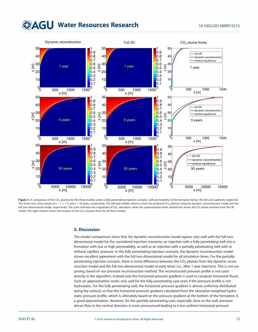
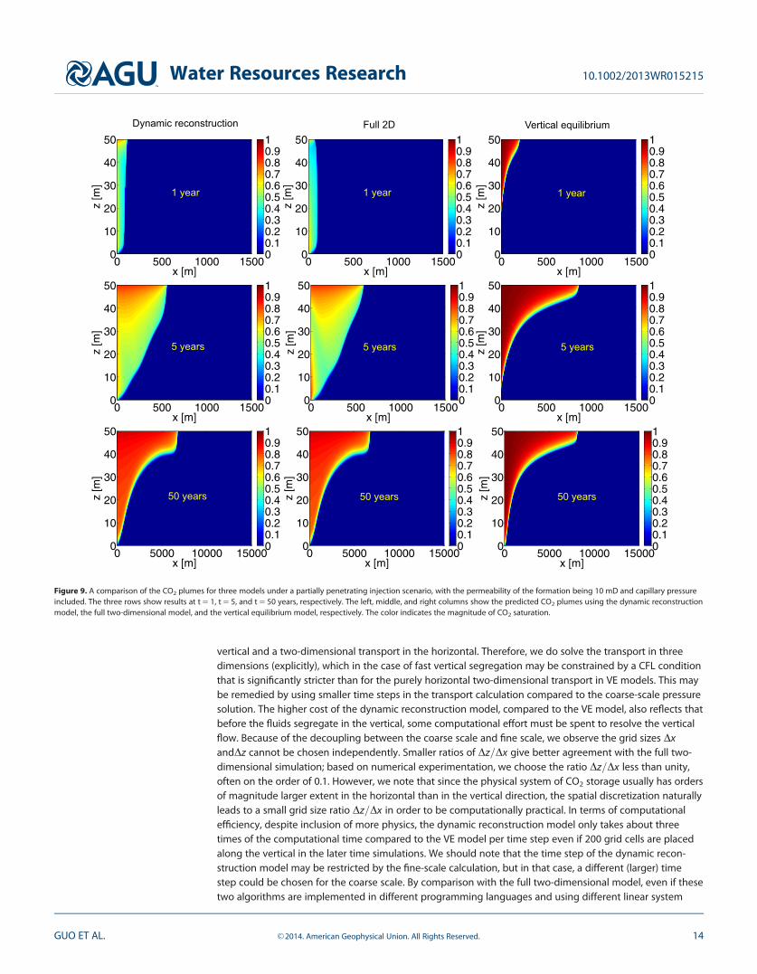
Finally, a CO2 plume comparison of the three models for a partially penetrating injection scenario with capil-lary pressure taken into account is shown in Figure 9. Similar to the case without capillary pressure, thedynamic reconstruction shows very good agreement with the full two-dimensional model except at the ear-liest time (i.e., after 1 year injection). But, again, the VE model gives much worse results than the dynamicreconstruction model in that case. We should note that although the VE model is still quite different fromthe other two models, it gives better results compared to the case without capillary pressure. In particular,the VE model tends to overestimate the outer-most extent of the CO2 plume less when capillary pressure isincluded.

0 500 1000 15000

10

20

30

40

50

x [m]

z [m

]

full 2Ddynamic reconstructionvertical equilibrium

0 5000 10000 150000

10

20

30

40

50

x [m]

z [m

]full 2Ddynamic reconstructionvertical equilibrium

x [m]

z [m

]

0 5000 10000 150000

10

20

30

40

50

00.10.20.30.40.50.60.70.80.91

x [m]

z [m

]

0 5000 10000 150000

10

20

30

40

50

00.10.20.30.40.50.60.70.80.91

x [m]

z [m

]

0 500 1000 15000

10

20

30

40

50

00.10.20.30.40.50.60.70.80.91

x [m]

z [m

]

0 500 1000 15000

10

20

30

40

50

00.10.20.30.40.50.60.70.80.91

x [m]z

[m]

0 500 1000 15000

10

20

30

40

50

00.10.20.30.40.50.60.70.80.91

x [m]

z [m

]

0 500 1000 15000

10

20

30

40

50

00.10.20.30.40.50.60.70.80.91

0 500 1000 15000

10

20

30

40

50

x [m]

z [m

]


1 year 1 year 1 year

5 years 5 years 5 years


Dynamic reconstruction Full 2D CO2 plume fronts

Figure 6. A comparison of the CO2 plumes for the three models under a fully penetrating injection scenario, with the permeability of the formation being 10 mD and capillarityneglected. The three rows show results at t 5 1, t 5 5, and t 5 50 years, respectively. Note the scale on the x axis is 10 times larger in the third row. The left and middle columns showthe predicted CO2 plumes using the dynamic reconstruction model and the full two-dimensional model, respectively. The color indicates the magnitude of CO2 saturation, while thesuperimposed red (white for the third row) dashed line shows the CO2-brine interface from the VE model. The right column shows the location of the CO2 invasion front for all threemodels.



5. Discussion

The model comparisons show that the dynamic reconstruction model agrees very well with the full two-dimensional model for the considered injection scenarios: an injection with a fully penetrating well into aformation with low or high permeability, as well as an injection with a partially penetrating well with orwithout capillary pressure. In the fully penetrating injection scenario, the dynamic reconstruction modelshows excellent agreement with the full two-dimensional model for all simulation times. For the partiallypenetrating injection scenario, there is some difference between the CO2 plumes from the dynamic recon-struction model and the full two-dimensional model at early times (i.e., after 1 year injection). This is not sur-prising, based on our pressure reconstruction method. The reconstructed pressure profile is not useddirectly in the algorithm, instead only the horizontal pressure gradient is used to compute horizontal fluxes.Such an approximation works very well for the fully penetrating case even if the pressure profile is nothydrostatic. For the fully penetrating well, the horizontal pressure gradient is almost uniformly distributedalong the vertical, so that the horizontal pressure gradient calculated from the saturation-weighted hydro-static pressure profile, which is ultimately based on the pressure gradient at the bottom of the formation, isa good approximation. However, for the partially penetrating case, especially close to the well, pressure-driven flow in the vertical direction is more pronounced leading to a less uniform horizontal pressure

0 5000 10000 150000

10

20

30

40

50

x [m]

z [m

]


x [m]

z [m

]

0 5000 10000 150000

10

20

30

40

50

00.10.20.30.40.50.60.70.80.91

x [m]

z [m

]

0 5000 10000 150000

10

20

30

40

50

00.10.20.30.40.50.60.70.80.91

x [m]

z [m

]

0 500 1000 15000

10

20

30

40

50

00.10.20.30.40.50.60.70.80.91

x [m]z

[m]

0 500 1000 15000

10

20

30

40

50

00.10.20.30.40.50.60.70.80.91

x [m]

z [m

]

0 500 1000 15000

10

20

30

40

50

00.10.20.30.40.50.60.70.80.91

x [m]

z [m

]

0 500 1000 15000

10

20

30

40

50

00.10.20.30.40.50.60.70.80.91

0 500 1000 15000

10

20

30

40

50

x [m]

z [m

]


0 500 1000 15000

10

20

30

40

50

x [m]

z [m

]






Figure 7. A comparison of the CO2 plumes for the three models under a fully penetrating injection scenario, with permeability of the formation being 100 mD and capillarity neglected.The three rows show results at t 5 1, t 5 5, and t 5 50 years, respectively. The left and middle columns show the predicted CO2 plumes using the dynamic reconstruction model and thefull two-dimensional model, respectively. The color indicates the magnitude of CO2 saturation, while the superimposed white dashed line shows the CO2-brine interface from the VEmodel. The right column shows the location of the CO2 invasion front for all three models.



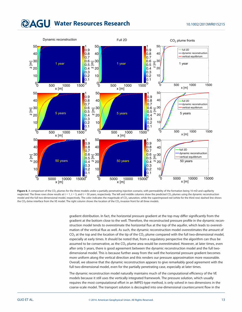
gradient distribution. In fact, the horizontal pressure gradient at the top may differ significantly from thegradient at the bottom close to the well. Therefore, the reconstructed pressure profile in the dynamic recon-struction model tends to overestimate the horizontal flux at the top of the aquifer, which leads to overesti-mation of the vertical flux as well. As such, the dynamic reconstruction model overestimates the amount ofCO2 at the top and the location of the tip of the CO2 plume compared with the full two-dimensional model,especially at early times. It should be noted that, from a regulatory perspective the algorithm can thus beassumed to be conservative, as the CO2 plume area would be overestimated. However, at later times, evenafter only 5 years, there is good agreement between the dynamic reconstruction model and the full two-dimensional model. This is because further away from the well the horizontal pressure gradient becomesmore uniform along the vertical direction and this renders our pressure approximation more reasonable.Overall, we observe that the dynamic reconstruction appears to give remarkably good agreement with thefull two-dimensional model, even for the partially penetrating case, especially at later times.

The dynamic reconstruction model naturally maintains much of the computational efficiency of the VEmodels because it still uses the vertically integrated framework. The pressure solution, which usuallyrequires the most computational effort in an IMPES-type method, is only solved in two dimensions in thecoarse-scale model. The transport solution is decoupled into one-dimensional countercurrent flow in the

0 5000 10000 150000

10

20

30

40

50

x [m]

z [m

]full 2Ddynamic reconstructionvertical equilibrium

x [m]

z [m

]

0 5000 10000 150000

10

20

30

40

50

00.10.20.30.40.50.60.70.80.91

x [m]

z [m

]

0 5000 10000 150000

10

20

30

40

50

00.10.20.30.40.50.60.70.80.91

x [m]

z [m

]

0 500 1000 15000

10

20

30

40

50

00.10.20.30.40.50.60.70.80.91

x [m]z

[m]

0 500 1000 15000

10

20

30

40

50

00.10.20.30.40.50.60.70.80.91

x [m]

z [m

]

0 500 1000 15000

10

20

30

40

50

00.10.20.30.40.50.60.70.80.91

x [m]

z [m

]

0 500 1000 15000

10

20

30

40

50

00.10.20.30.40.50.60.70.80.91

0 500 1000 15000

10

20

30

40

50

x [m]

z [m

]


0 500 1000 15000

10

20

30

40

50

x [m]

z [m

]






Figure 8. A comparison of the CO2 plumes for the three models under a partially penetrating injection scenario, with permeability of the formation being 10 mD and capillarityneglected. The three rows show results at t 5 1, t 5 5, and t 5 50 years, respectively. The left and middle columns show the predicted CO2 plumes using the dynamic reconstructionmodel and the full two-dimensional model, respectively. The color indicates the magnitude of CO2 saturation, while the superimposed red (white for the third row) dashed line showsthe CO2-brine interface from the VE model. The right column shows the location of the CO2 invasion front for all three models.



vertical and a two-dimensional transport in the horizontal. Therefore, we do solve the transport in threedimensions (explicitly), which in the case of fast vertical segregation may be constrained by a CFL conditionthat is significantly stricter than for the purely horizontal two-dimensional transport in VE models. This maybe remedied by using smaller time steps in the transport calculation compared to the coarse-scale pressuresolution. The higher cost of the dynamic reconstruction model, compared to the VE model, also reflects thatbefore the fluids segregate in the vertical, some computational effort must be spent to resolve the verticalflow. Because of the decoupling between the coarse scale and fine scale, we observe the grid sizes DxandDz cannot be chosen independently. Smaller ratios of Dz=Dx give better agreement with the full two-dimensional simulation; based on numerical experimentation, we choose the ratio Dz=Dx less than unity,often on the order of 0.1. However, we note that since the physical system of CO2 storage usually has ordersof magnitude larger extent in the horizontal than in the vertical direction, the spatial discretization naturallyleads to a small grid size ratio Dz=Dx in order to be computationally practical. In terms of computationalefficiency, despite inclusion of more physics, the dynamic reconstruction model only takes about threetimes of the computational time compared to the VE model per time step even if 200 grid cells are placedalong the vertical in the later time simulations. We should note that the time step of the dynamic recon-struction model may be restricted by the fine-scale calculation, but in that case, a different (larger) timestep could be chosen for the coarse scale. By comparison with the full two-dimensional model, even if thesetwo algorithms are implemented in different programming languages and using different linear system

x [m]

z [m

]

0 5000 10000 150000

10

20

30

40

50

00.10.20.30.40.50.60.70.80.91

x [m]

z [m

]

0 5000 10000 150000

10

20

30

40

50

00.10.20.30.40.50.60.70.80.91

x [m]

z [m

]

0 500 1000 15000

10

20

30

40

50

00.10.20.30.40.50.60.70.80.91

x [m]

z [m

]

0 500 1000 15000

10

20

30

40

50

00.10.20.30.40.50.60.70.80.91

x [m]z

[m]

0 500 1000 15000

10

20

30

40

50

00.10.20.30.40.50.60.70.80.91

x [m]

z [m

]

0 500 1000 15000

10

20

30

40

50

00.10.20.30.40.50.60.70.80.91

x [m]

z [m

]

0 5000 10000 150000

10

20

30

40

50

00.10.20.30.40.50.60.70.80.91

x [m]

z [m

]

0 500 1000 15000

10

20

30

40

50

00.10.20.30.40.50.60.70.80.91

x [m]

z [m

]

0 500 1000 15000

10

20

30

40

50

00.10.20.30.40.50.60.70.80.91




Dynamic reconstruction Full 2D Vertical equilibrium

Figure 9. A comparison of the CO2 plumes for three models under a partially penetrating injection scenario, with the permeability of the formation being 10 mD and capillary pressureincluded. The three rows show results at t 5 1, t 5 5, and t 5 50 years, respectively. The left, middle, and right columns show the predicted CO2 plumes using the dynamic reconstructionmodel, the full two-dimensional model, and the vertical equilibrium model, respectively. The color indicates the magnitude of CO2 saturation.



solvers, we observe that the dynamic reconstruction model is at least 1 order of magnitude faster for mostcases. Overall, this implies that the dynamic reconstruction model captures more physics than the VE mod-els while still maintaining much of the computational advantages over full multidimensional models.

Because the purpose of this paper is to introduce the new dynamic reconstruction algorithm, we have usedrelatively simple example problems to demonstrate the concept and to show that the algorithm appears togive significant improvements compared to the VE model while retaining many of its attractive features. Allof the example problems involve homogeneous, horizontal, isotropic formations with uniform thicknessinvolving two immiscible fluid phases. The design of the algorithm does not explicitly rely on these simplifi-cations. Thus, we expect that inclusion of material heterogeneities, geometric complexities, and phase inter-actions including dissolution and miscible transport is possible within our general framework. However, wehave not implemented those extensions, so their efficacy remains to be studied.

6. Conclusion

A novel multiscale method for modeling CO2 storage has been presented in this paper, based on verticallyintegrated equations coupled with a dynamic reconstruction of saturation and pressure in the vertical direc-tion. This differs from the usual vertically integrated models, which assume vertical equilibrium and there-fore do not include any vertical flow dynamics. For the example problems studied, the new model showsexcellent agreement with full multidimensional models, and shows significant improvements over VerticalEquilibrium (VE) models for cases when vertical equilibrium is not an appropriate assumption. The newmodel also matches the VE results in the limit of very fast segregation times, which are the cases for whichVE is applicable. Overall, the dynamic reconstruction model provides a new multiscale framework for large-scale CO2 storage problems which extends the scope of applicability of vertically integrated models. Exten-sions to include additional fine-scale physics, such as vertical heterogeneity and fluid solubility, should alsobe possible although we have not yet explored these in any depth.

The dynamic reconstruction model maintains many of the computational advantages of the VE model andtherefore requires much less computational effort compared to full multidimensional models. The ability tocapture more physics while still maintaining a low level of computational effort makes these dynamicreconstruction models attractive for computational studies of large-scale CO2 storage systems where thevertical dynamics of CO2 and brine are important.

ReferencesBandilla, K. W., M. A. Celia, T. R. Elliot, M. Person, K. Ellet, J. Rupp, C. Gable, and M. Dobossy (2012), Modeling carbon sequestration in the Illi-

nois Basin using a vertically-integrated approach, Comput. Visualization Sci., (15), 39–51.Bear, J. (1972), Dynamics of Fuids in Porous Media, Elsevier, N. Y.Benson, S., P. Cook, J. Anderson, and S. Bachu (2005), Underground geological storage, in Carbon Dioxide Capture and Storage, Intergovern-

mental Panel on Climate Change Special Report, edited by B. Metz et al., pp. 95–276, Cambridge Univ. Press, N. Y.Court, B., K. W. Bandilla, M. A. Celia, A. Janzen, M. Dobossy, and J. M. Nordbotten (2012), Applicability of vertical-equilibrium and sharp-

interface assumptions in CO2 sequestration modeling, Int. J. Green. Gas. Con., 10, 134–147.Dentz, M., and D. M. Tartakovsky (2009), Abrupt-interface solution for carbon dioxide injection into porous media, Transp. Porous Media,

79(1), 15–27.Doster, F., E. Keilegavlen, and J. M. Nordbotten (2014), A robust implicit pressure explicit mass method for multi-phase multi-component

flow including capillary pressure and buoyancy, in Computational Models for CO2 Sequestration and Compressed Air Energy Storage,edited by Ralfid al Khoury, and Jochen Bundschuh, Taylor and Francis Group/CRC Press, Boca Raton, Fla.

Gasda, S. E., J. M. Nordbotten, and M. A. Celia (2009), Vertical equilibrium with sub-scale analytical methods for geological CO2 sequestra-tion, Comput. Geosci., 13(4), 469–481.

Gasda, S. E., J. M. Nordbotten, and M. A. Celia (2011), Vertically averaged approaches for CO2 migration with solubility trapping, WaterResour. Res., 47, W05528, doi:10.1029/2010WR009075.

Gasda, S. E., J. M. Nordbotten, and M. A. Celia (2012a), Application of simplified models to CO2 migration and immobilization in large-scalegeological systems, Int. J. Green. Gas. Con., 9, 72–84.

Gasda, S. E., H. M. Nilsen, H. K. Dahle, and W. G. Gray (2012b), Effective models for CO2 migration in geological systems with varying topog-raphy, Water Resour. Res., 48, W10546, doi:10.1029/2012WR012264.

Hesse, M. A., H. A. Tchelepi, B. J. Cantwell, and F. M. Orr (2007), Gravity currents in horizontal porous layers: transition from early to late self-similarity, J. Fluid Mech., 577, 363–383.

Hesse, M. A., F. M. Orr, and H. A. Tchelepi (2008), Gravity currents with residual trapping, J. Fluid Mech., 611, 35–60.Huppert, H. E., and A. W. Woods (1995), Gravity-driven flows in porous layers, J. Fluid Mech., 292, 55–69.Juanes, R., C. W. MacMinn, and M. L. Szulczewski (2010), The footprint of the CO2 plume during carbon dioxide storage in saline aquifers:

Storage efficiency for capillary trapping at the basin scale, Transp. Porous Media, 82(1), 19–30.Lyle, S., H. E. Huppert, M. Hallworth, M. Bickle, and A. Chadwick (2005), Axisymmetric gravity currents in a porous medium, J. Fluid Mech.,

543, 293–302.

AcknowledgementsThis work was supported in part by theNational Science Foundation undergrant EAR-0934722; the Department ofEnergy under grant DE-FE0009563; theEnvironmental Protection Agencyunder Cooperative Agreement RD-83438501; and the Carbon MitigationInitiative at Princeton University. Theauthors would like to acknowledgehelpful discussions with J. Nordbottenand S. Gasda.



http://dx.doi.org/10.1029/2010WR009075

http://dx.doi.org/10.1029/2012WR012264

Nilsen, H. M., P. A. Herrera, M. Ashraf, I. Ligaarden, M. Iding, C. Hermanrud, K.-A. Lie, J. M. Nordbotten, H. K. Dahle, and E. Keilegavlen (2011),Field-case simulation of CO2-plume migration using vertical-equilibrium models, Energy Procedia, 4, 3801–3808.

Nordbotten, J. M., and M. A. Celia (2006), Similarity solutions for fluid injection into confined aquifers, J. Fluid Mech., 561, 307–327.Nordbotten, J. M., and M. A. Celia (2012), Geological Storage of CO2: Modeling Approaches for Large-Scale Simulation, John Wiley, Hoboken,

N. J.Nordbotten, J. M., M. A. Celia, and S. Bachu (2005), Injection and storage of CO2 in deep saline aquifers: Analytical solution for CO2 plume

evolution during injection, Transp. Porous Media, 58(3), 339–360.Pacala, S., and R. Socolow (2004), Stabilization wedges: Solving the climate problem for the next 50 years with current technologies, Sci-

ence, 305(5686), 968–972.Pruess, K. (2005), The TOUGH codes—A family of simulation tools for multiphase flow and transport processes in permeable media, Vadose

Zone J., 3(3), 738–746.Schlumberger (2010), ECLIPSE Technical Description, Schlumberger, Houston, Tex.Vella, D., and H. E. Huppert (2006), Gravity currents in a porous medium at an inclined plane, J. Fluid Mech., 555, 353–362.White, M. D., and M. Oostrom (1997), Subsurface Transport Over Multiple Phases, Richland, Wash.Woods, A. W., and R. Mason (2000), The dynamics of two-layer gravity-driven flows in permeable rock, J. Fluid Mech., 421, 83–114.Zyvoloski, G. A., B. A. Robinson, Z. V. Dash, and L. L. Trease (1997), Summary of the models and methods for the FEHM application—A finite

element heat-and mass-transfer code, Los Alamos Natl. Lab., Los Alamos, N. M.



publications - university of arizonaboguo/pdfs/publications/2014_gu… · · 2017-08-27scenarios...

Documents