Hyper-parameter selection in non-quadratic regularization-based radar image formation

Özge Batua and Müjdat Çetina,b

aFaculty of Engineering and Natural Sciences,

Sabancı University, Orhanlı, Tuzla 34956 İstanbul, Turkey bLaboratory for Information and Decision Systems,

Massachusetts Institute of Technology, Cambridge, MA 02139, USA

ABSTRACT

We consider the problem of automatic parameter selection in regularization-based radar image formation techniques. It has previously been shown that non-quadratic regularization produces feature-enhanced radar images; can yield superresolution; is robust to uncertain or limited data; and can generate enhanced images in non-conventional data collection scenarios such as sparse aperture imaging. However, this regularized imaging framework involves some hyper-parameters, whose choice is crucial because that directly affects the characteristics of the reconstruction. Hence there is interest in developing methods for automatic parameter choice. We investigate Stein’s unbiased risk estimator (SURE) and generalized cross-validation (GCV) for automatic selection of hyper-parameters in regularized radar imaging. We present experimental results based on the Air Force Research Laboratory (AFRL) “Backhoe Data Dome,” to demonstrate and discuss the effectiveness of these methods.

Keywords: synthetic aperture radar, hyper-parameter selection, sparse-aperture imaging, feature-enchanced imaging, inverse problems

1. INTRODUCTION Conventional image formation techniques for synthetic aperture radar (SAR) suffer from low resolution, speckle and sidelobe artifacts. These effects pose challenges for SAR images when used in automatic target detection and recognition tasks. Recently, new SAR image formation algorithms have been proposed to produce high quality images which provide increased resolution and reduced artifacts [1,2,3]. We consider the non-quadratic regularization-based approach of [1] which aims at providing feature-enhanced SAR images. The idea behind this approach is to emphasize appropriate features by means of regularizing the solution. In fact, regularization methods are well known and widely used for real-valued image restoration and reconstruction problems. However SAR imaging involves some difficulties in application of these methods. As an example, SAR involves complex-valued reflectivities. Considering and addressing such difficulties, extensions of real-valued non-quadratic regularization methods have been developed for SAR imaging.

Regularization methods, in general, try to balance the fidelity to data and prior knowledge to obtain a stable solution. This stability is ensured through a scalar parameter which is called regularization parameter or hyper-parameter. Selection of this parameter is another problem in a regularization framework. There exist several approaches which have been mostly practised in quadratic regularization methods such as Tikhonov regularization. Recently, non-quadratic methods have acquired greater importance thanks to their property of preserving useful features such as edges. Hence there is interest in developing methods for automatic parameter choice in the non-quadratic setting.

____________________________________________

Further author information: Özge Batu: E-mail: ozgebatu@su.sabanciuniv.edu Müjdat Çetin: E-mail: mcetin@sabanciuniv.edu, mcetin@mit.edu

We consider Stein’s unbiased risk estimator (SURE) and generalized cross-validation (GCV) for parameter selection in non-quadratic regularization-based radar imaging. They have been both used in problems with quadratic constraints [4,5] but the experiments for non-quadratic methods are limited [6]. We propose their use in the regularization-based SAR image formation framework. We present the effectiveness of SURE and GCV through our experiments based on the Air Force Research Laboratory (AFRL) “Backhoe Data Dome” [7].

2. REGULARIZATION-BASED SAR IMAGING For feature-enhanced image formation we consider an approach based on non-quadratic regularization [1]. The framework of [1] relies on the SAR observation process expressed in the following form:

y Hf w= + (1)

where H represents a complex-valued discrete SAR operator, w stands for additive noise, y and f are data and the reflectivity field, respectively. Here we prefer to use the conventional image as the input data, hence the technique works as a deconvolution method. In this framework, SAR image reconstruction problem is formulated as the following optimization problem

( )ˆ arg minf

f J f= . (2)

One choice for ( )J f , which we consider here, has the following form:

( ) 2

2

p

pJ f y Hf fλ= − + (3)

where . p

p denotes the pl -norm and λ is a scalar parameter. The first term in the objective function (3) is a data

fidelity term, which incorporates the SAR observation model (1), and thus information about the observation geometry. The second term in (3) incorporates prior information reflecting the nature of the field f , and is aimed at enhancing point-based features. Additional terms like a smoothness penalty on f can be employed in this framework to emphasize other characteristics of the field. However, in fact, many object recognition methods rely on locations of dominant point scatterers extracted from SAR images. Therefore we choose the cost function ( )J f to be as in (3) throughout this work, and thus produce images in which point-based features are enhanced. It has been known that minimum pl -norm reconstruction with 1p ≤ provides localized energy concentrations in the resultant image. In such images, most elements are forced to be small, on the other hand, a few are allowed to have very large values. With respect to 2l -norm reconstruction this approach favors a field with smaller number of dominant scatterers. This type of constraint aims to suppress artifacts and increase the resolvability of scatterers.

To avoid the problems due to nondifferentiability of the objective function around the origin, a smooth approximation to the pl -norm is used, and the objective function takes the following form

( ) ( )2

2 2

21

pn

ii

J f y Hf fλ β=

= − + +∑ (4)

where if denotes the ith element of f , n is the number of pixels in f , and β is a small scalar. The estimate f̂ is the solution of the following equation:

( )( ) 1ˆ ˆT Tf H H W f H yβλ−

= + (5)

where ( )ˆW fβ is a diagonal weight matrix whose ith diagonal element is ( )( )2 22 p

ip f β−

+ . The weight matrix acts

in the following manner: if there is a scattering object in the field of interest then if ’s will be large, and thus

corresponding elements of ( )ˆW fβ will be small and allowing large intensities. Otherwise, elements of ( )ˆW fβ will

be large and suppress the energy concentrations at that location.

The expression in (5) is still nonlinear and no closed form solution exists. An iterative procedure can handle the nonlinearity and results in the formulation:

( )( ) 11ˆ ˆk T k Tf H H W f H yβλ

−+ = + (6)

where ˆ kf is the estimate calculated in the kth iteration. In this way, the problem becomes linear at each individual step.

3. HYPER-PARAMETER SELECTION METHODS

The objective function in (4) contains a scalar parameter λ which has a role in determining the behavior of the

reconstructed field f̂ . Small parameter values makes data fidelity term; i.e. first term in (4), dominate the solution whereas large values of λ impose greater importance to prior term and ensure that point-based features are enhanced. To choose λ in a data-driven way, we consider two methods: Stein’s unbiased risk estimator (SURE) and generalized cross-validation (GCV). 3.1 Stein’s unbiased risk estimator

Stein’s unbiased risk estimator (SURE) is developed by Stein [4] for parameter selection in linear regression and it has been adapted for the solution of inverse problems. SURE aims to minimize the predictive risk:

22

2 2

1 1 ˆp Hf Hfn nλ λ= − (7)

which is basically mean squared norm of the predictive error. Here f̂λ represents the solution obtained with parameter

λ and f is the true, unknown reflectivity field. In fact, the predictive error is not computable since f is unknown, but it can be estimated using available information.

It has been shown that [4] an unbiased estimator of (7) is

( ) ( ) ( )2

2 22

1

1 2 n

i ii

U r r yn n

σλ λ λ σ=

= − ∂ ∂ +∑ (8)

where ( ) ˆr Hf yλλ = − and 2σ is the varience of the noise w . ( )U λ is called Stein’s unbiased risk estimator (SURE). It has been shown that [6] SURE takes the following form after some intermediate operations:

( ) ( ) ( )2

2 22

1 2U r trace An n λ

σλ λ σ= + − (9)

where 1ˆ̂

Tff

A HJ Hλ−= and 2 2

ˆˆˆ

ffJ J f= ∂ ∂ . For the cost function given in (4),

( )

( )4 22 2

ˆ̂ˆ ˆ1

pT

i iffJ H H diag p f p fλ β β

−⎛ ⎞⎛ ⎞ ⎛ ⎞= + + − +⎜ ⎟⎜ ⎟ ⎜ ⎟⎜ ⎟⎝ ⎠ ⎝ ⎠⎝ ⎠. (10)

The method chooses the parameter which minimizes ( )U λ . Numerical results suggest that λ which minimizes the

predictive risk will yield a small value for the estimation error of f . It is also noteworthy that SURE requires prior knowledge on the noise, namely its variance, in the model (1).

3.2 Generalized cross-validation

Another parameter selection method is generalized cross-validation (GCV) which is also an estimator for the predictive risk (7) and has the advantage of being independent of the prior knowledge on the noise w . The idea of GCV is as follows: choose λ such that the solution obtained in the presence of a missing data point predicts the missing point in a proper manner, when averaged over all ways of removing a point. The method intends to minimize the GCV function:

( )( )( )

212

21

n

n

rGCV

trace I Aλ

λλ =

⎡ ⎤−⎣ ⎦ (11)

where ( )r λ and Aλ are the same quantities in the SURE setting.

4. NUMERICAL OPTIMIZATION TOOLS Both SURE and GCV involve computational difficulties when considered in the framework of non-quadratic regularization.1 First of all, they require the computation of the matrix Aλ through large scale matrix multiplications and

inversions which are not practical at all. Then they require the solution of an optimization problem over λ . To clarify the implementation details we discuss some numerical tools we use in the solution.

We note that all the matrix vector products in (6) are actually carried out by convolution operations (in the Fourier domain) such that there is no need to construct the convolution matrix H and deal with memory-intensive matrix operations. However convolutional operations do not help for evaluation of the GCV cost in (11) since it involves the trace of the matrix Aλ . Instead of calculating Aλ one can approximate the trace of Aλ by means of randomized trace estimation [8]. If q is a white noise vector with zero mean and unit variance, then an unbiased estimator for

( )trace Aλ can be constructed based on the random variable ( ) Tt q A qλλ = . The trace estimate can be computed as

follows: first generate a number of independent realizations of q and compute ( )t λ for each, and then take the

arithmetic mean of the random variable ( )t λ to be the trace estimate. In our experiments we also observed that the

randomized trace estimate approaches successfully to the actual trace. Note that we compute ( )t λ using convolution

operations without explicitly constructing the matrix Aλ . This method makes the computation of the GCV function

feasible for a given λ . However there is still the issue of finding the minimizers of the GCV cost.

One way to find the minimum of the GCV cost is brute-force searching. After determining a reasonable range for values of λ , the range is divided into grids and solution is obtained for each grid point. Then, λ which gives the smallest function value is selected as the minimizer. Since this may yield extensive computations, appropriate optimization methods can be employed instead. Most of the methods are based on gradient information of the functions. However evaluation of the gradient of GCV appears to be a problem. Due to the complicated dependence of (9) and (11) on λ

through f̂λ , it is not straightforward to compute the gradient. This difficulty leads us consider two different approaches: derivative-free optimization techniques and numerical computations of the gradient.

1In this section we only mention GCV for convenience, all the procedure is identical for SURE.

Golden section search is a one dimesional optimization method and does not require the gradient information [9]. This approach assumes that the function is unimodal (at least in an interval [ ],a b ), which is the case for GCV cost according

to our observations. We first determine an interval [ ],a b for λ and choose two initial test points 1λ and 2λ in interval

such that 1 2λ λ< . Using those particular choices of λ ’s we find the solution f̂λ and the GCV value for each. After

evaluating GCV( 1λ ) and GCV( 2λ ) one of the following cases produces a new interval which is the subset of [ ],a b .

Case 1: If GCV( 1λ ) > GCV( 2λ ), then the new interval is [ ]1,bλ .

Case 2: If GCV( 1λ ) ≤ GCV( 2λ ), then the new interval is [ ]2,a λ .

As a result, the interval is shrinked and two new test points are selected such that they divide the interval into the Golden section. Golden ratio requires:

length of whole interval length of larger part of interval

length of larger part of interval length of smaller part of interval=

Thus the algorithm ends up with an interval of uncertainity; i.e. it does not provide a single point as the minimizer.

Since the challenge is the exact derivative computation we also consider approximating derivatives through finite differences. With an initial λ at hand we move to a close point λ ε+ and find the solution f̂λ and the GCV value for

each and calculate the finite difference of GCV at λ . Once the approximated gradient is found one can choose one of the line search algorithms to obtain the optimal point [10]. Since we don’t want to deal with second order derivatives we choose a line search algorithm which uses a descent direction and thus does not require second order derivatives. To determine the step length one can use a step-length selection algorithm such as interpolation or use backtracking. In our experiments we apply the backtracking algorithm. The algorithm takes a step and checks the Armijo condition; if it is not satisfied, the step length is reduced and Armijo condition is checked again. The backtracking continues until a step length satisfying Armijo condition is found. Initial λ to be used in this procedure may be selected using a computationally less expensive method. For this task we employ the parameter selection approach in [11]. This method suggests the regularization parameter to be selected as 2 log nλ σ= in a basis pursuit framework. Here σ is the standard deviation of the noise in (1) and n is the length of the noise vector.

5. EXPERIMENTS We present 2D image reconstruction experiments based on the AFRL “Backhoe Data Dome and Visual-D challange problem” which consists of simulated wideband (7-13 GHz), full polarization, complex backscatter data from a backhoe vehicle in free space [7]. The backscatter data are available over a full upper 2π steradian viewing hemisphere. In our experiments, we use VV polarization data, centered at 10 GHz, and with an azimuthal span of 110° (centered at 45°). Advanced imaging strategies have enabled resolution-enhanced wide angle SAR imaging. We consider the point-enhanced composite imaging technique [12] and show experimental results in this framework. For composite imaging, we use 19 subapertures, with azimuth centers at 0°, 5°, …, 90°, and each with an azimuthal width of 20°. We consider two different bandwidths: 500 MHz and 1 GHz. For each of these bandwidths, we consider data with three different signal-to-noise ratios: 25 dB, 20 dB and 10 dB.

To be able to carry out some quantitative analysis, we have also created a synthetic problem which simulates imaging of a point-like scattering field in a narrow-angle imaging scenario. The field consists of five scatterers. We simulate SAR data with 1 GHz bandwidth and 25 dB SNR. We choose 1p = in (3). The underlying true scene, the conventional reconstruction and reconstructed images with different regularization parameters are shown in Figure 1. In these images it is obviously seen that small parameter values are insufficient to enhance point-based features whereas large parameter values overregularize the solution and cause some scatterers to be unobservable. The image in Figure 1(d) is obtained

(ab)

(cde)

Figure 1. SAR images of a synthetic problem. (a) Underlying field consisting of point-like scatterers. (b) Conventional SAR image of the field. (c) Point-enhanced image with small λ. (d) Point-enhanced image with λ selected by GCV. (e) Point-enhanced image with large λ.

using λ selected by the GCV method. It appears to be an accurate reconstruction in the sense that it preserves all the five scatterers and does not cause significant artifacts.

In Figure 2, we show the SURE (solid, blue) and GCV (dashed, green) curves for the synthetic problem. The red (dash-

dotted) curve indicates the estimation error which we define as 2

2

1 f̂ fn

− . The minimum point for each curve is

enclosed by a square. Both SURE and GCV appear to be leading to slight under-regularization. Generally, SURE tends to choose a smaller λ value than GCV does. In fact, both functions are quite flat around the minimum; hence they are not very sensitive therein. Fortunately, the estimation error is not very sharp around the minimum either; and therefore SURE and GCV give reasonable results in terms of the estimation error. We also show the choice of the method proposed by Chen [11], and it behaves like an over-regularizer for this problem setting. It can be used as the initial parameter in the optimization procedure. However, we cannot be sure about the behaivour of this method for different settings since it depends only on the standard deviation of the noise and the size of the problem. For example; it will not respond to changes in the experimental scenario such as bandwidth (and in turn range resolution).

We now demonstrate the behavior of Golden section search and numerical gradient descent method for optimization. In Figure 3, we show the paths displaying the progress of the methods. For Golden section search algorithm we choose the initial interval the same as the interval we choose in brute-force searching ( 2 010 ,10−⎡ ⎤⎣ ⎦ ). Golden section search

progresses quite fast and ends up with an interval requiring small number of reconstructions. Finding an interval of uncertainity does not appear to be a trouble since SURE and GCV curves are quite flat around the minimum. In Figure 3(b) we show the progress of the line search algorithm based on numerical gradient computation. Red cross markers indicate the λ value for progressing iterations (For better visualization we do not show the points at each iteration; instead one of every three iteration points is marked). For both methods the most important thing is the number of evaluations of GCV and SURE. Let’s consider a particular example, in which one would have to do 20 reconstructions to be able to determine λ with 25 10−± × variation in a brute-force search. We observe that it is possible to obtain the same precision with about 4 reconstructions in Golden search. Similarly, the numerical gradient computation-based algorithm provides almost the same advantage.

10-2 10-1 100

10-2

10-1

100

SUREGCVEstimation Error

Figure 2. SURE, GCV and Estimation Error curves for the synthetic image consisting of point-like scatterers. Minimum points are enclosed by squares. The point enclosed by a circle is the parameter selected by the method proposed in [11].

(a) (b)

Figure 3. Paths for optimization methods. (a) Right (green) and the left (red) endpoints of the intervals for Golden section search. (b) Improvement steps in line search for numerically computed gradient descent..

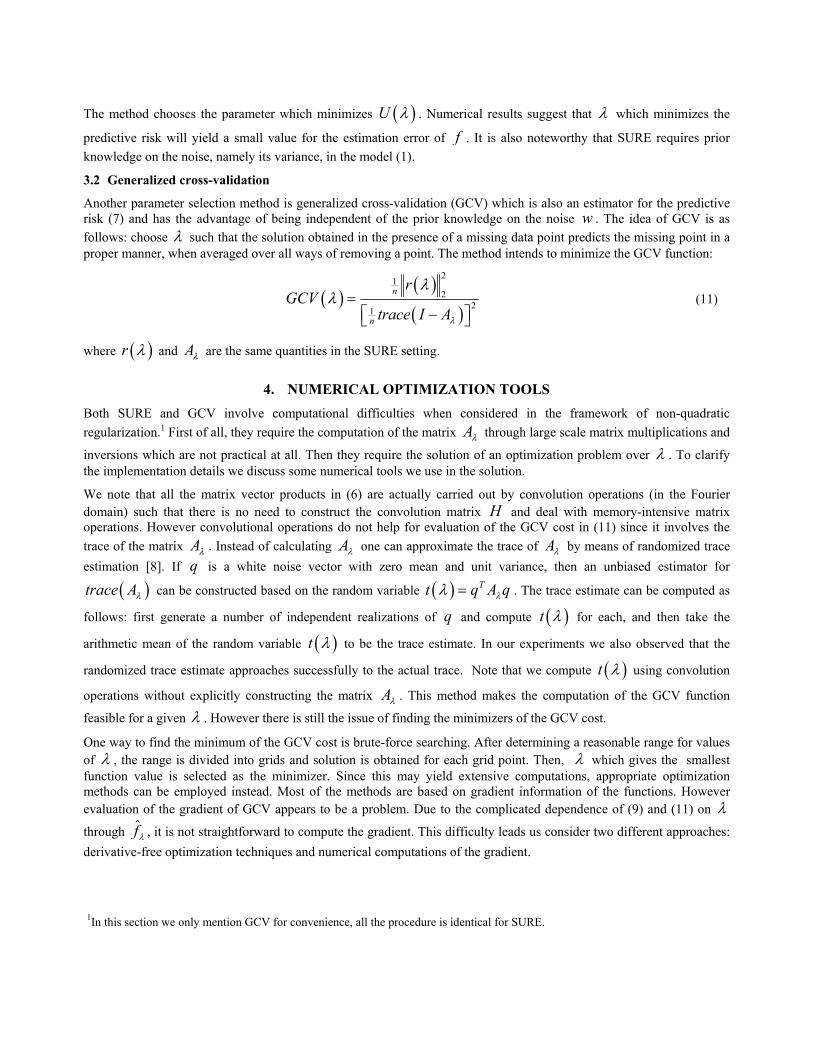
For backhoe data we cannot demostrate the mean square error of estimated f̂λ since the underlying field is not available a priori. Therefore we investigate the performance of the methods visually. First, we display the structure of SURE and GCV for backhoe data with bandwidth of 1 GHz and 500 MHz in Figure 4. A similar behavior to the synthetic problem is observed with this data. The curves are flat near the minimum, moreover the SURE curve is very flat for a wide range.

In Figure 5, we show the point-enhanced composite images obtained with different regularization parameters. Figure 5(c) is the image reconstructed using the parameter which is selected by GCV. Ideally, we would like to be able to observe the scattering centers of the backhoe in a good reconstruction. From this point of view GCV seems to serve the purpose. The under-regularized image in Figure 4(a) is dominated by artifacts and the over-regularized image in Figure 4(e) does not display the the structure of the backhoe correctly because of the unobservable scattering parts.

10-2

10-1

100

10-3

10-2

10-1

10-2

10-1

100

10-3

10-2

10-1

10-4 10-3 10-2 10-1 100

100

10-4 10-3 10-2 10-1 100

100

Figure 4. SURE (left) and GCV (right) curves for a subaperture image reconstructed from the data with SNR=20 dB and bandwidth of 1 GHz.

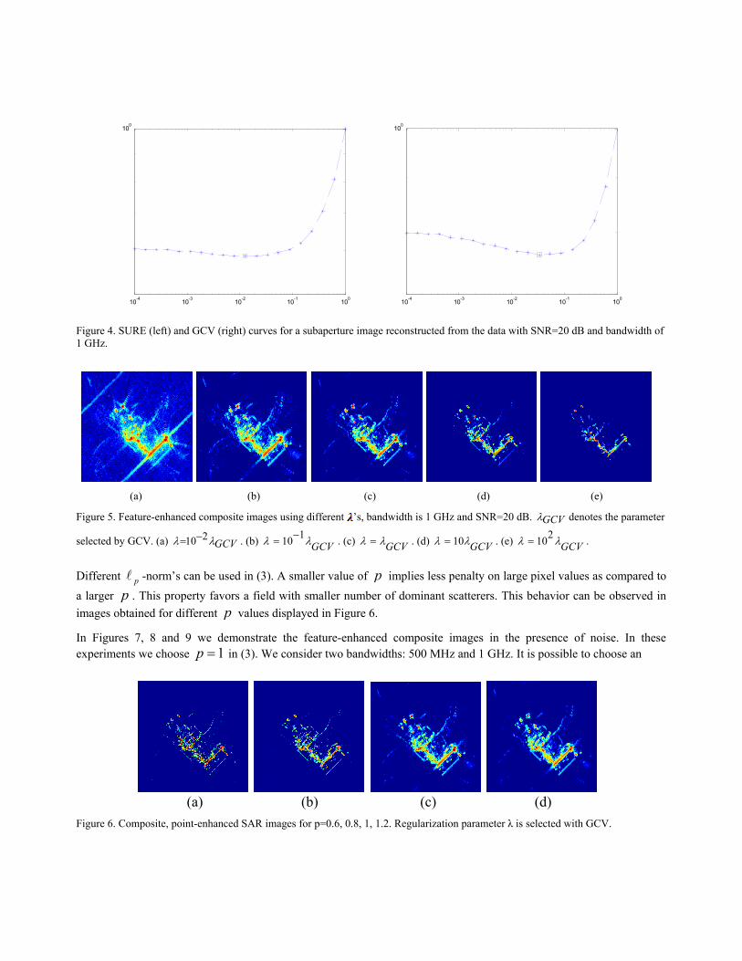
(a) (b) (c) (d) (e)

Figure 5. Feature-enhanced composite images using different ’s, bandwidth is 1 GHz and SNR=20 dB. GCVλ denotes the parameter

selected by GCV. (a) 210 GCVλ λ−= . (b) 110 GCVλ λ−= . (c) GCVλ λ= . (d) 10 GCVλ λ= . (e) 210 GCVλ λ= .

Different pl -norm’s can be used in (3). A smaller value of p implies less penalty on large pixel values as compared to a larger p . This property favors a field with smaller number of dominant scatterers. This behavior can be observed in images obtained for different p values displayed in Figure 6.

In Figures 7, 8 and 9 we demonstrate the feature-enhanced composite images in the presence of noise. In these experiments we choose 1p = in (3). We consider two bandwidths: 500 MHz and 1 GHz. It is possible to choose an

(a) (b) (c) (d) Figure 6. Composite, point-enhanced SAR images for p=0.6, 0.8, 1, 1.2. Regularization parameter λ is selected with GCV.

(a)

(b)

(c)

(d)

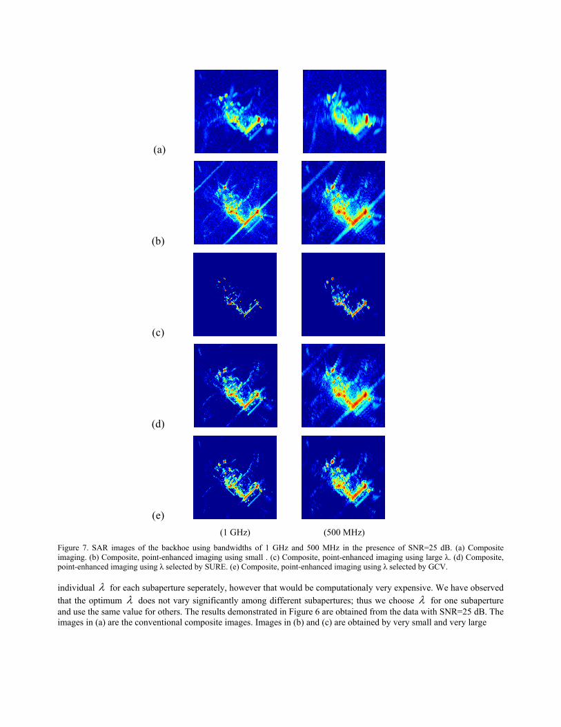
(e) (1 GHz) (500 MHz)

Figure 7. SAR images of the backhoe using bandwidths of 1 GHz and 500 MHz in the presence of SNR=25 dB. (a) Composite imaging. (b) Composite, point-enhanced imaging using small . (c) Composite, point-enhanced imaging using large λ. (d) Composite, point-enhanced imaging using λ selected by SURE. (e) Composite, point-enhanced imaging using λ selected by GCV.

individual λ for each subaperture seperately, however that would be computationaly very expensive. We have observed that the optimum λ does not vary significantly among different subapertures; thus we choose λ for one subaperture and use the same value for others. The results demonstrated in Figure 6 are obtained from the data with SNR=25 dB. The images in (a) are the conventional composite images. Images in (b) and (c) are obtained by very small and very large

(a)

(b)

(c)

(d)

(e) (1 GHz) (500 MHz)

Figure 8. SAR images of the backhoe using bandwidths of 1 GHz and 500 MHz in the presence of SNR=20 dB. (a) Composite imaging. (b) Composite, point-enhanced imaging using small λ. (c) Composite, point-enhanced imaging using large λ. (d) Composite, point-enhanced imaging using λ selected by SURE. (e) Composite, point-enhanced imaging using λ selected by GCV.

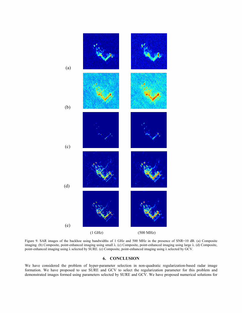
parameters, respectively. Results from SURE and GCV are shown in (d) and (e), respectively. The conventional composite images do not preserve the scatterers of the backhoe. Small and large parameters have the effects mentioned before and displayed in Figure 4. SURE and GCV are able to choose an acceptable λ value in different noise levels and resolutions. Figure 7 and 8 also shows feature-enhanced composite images for different parameters obtained from data with SNR=20 dB and SNR=10 dB, respectively. Obviously, sensitivity to parameter choice increases at lower SNR’s and SURE and GCV provide reasonable solutions.

(a)

(b)

(c)

(d)

(e) (1 GHz) (500 MHz)

Figure 9. SAR images of the backhoe using bandwidths of 1 GHz and 500 MHz in the presence of SNR=10 dB. (a) Composite imaging. (b) Composite, point-enhanced imaging using small λ. (c) Composite, point-enhanced imaging using large λ. (d) Composite, point-enhanced imaging using λ selected by SURE. (e) Composite, point-enhanced imaging using λ selected by GCV.

6. CONCLUSION We have considered the problem of hyper-parameter selection in non-quadratic regularization-based radar image formation. We have proposed to use SURE and GCV to select the regularization parameter for this problem and demonstrated images formed using parameters selected by SURE and GCV. We have proposed numerical solutions for

the optimization problems involved in these methods. We have observed that these methods lead to slight under-regularization but the parameter choices are reasonable. Regularized solutions become more sensitive to parameter choice at lower SNR’s, thus the role of the parameter selection methods gains significance.

ACKNOWLEDGEMENTS

This work was partially supported by the Scientific and Technological Research Council of Turkey under Grant 105E090, by the European Commission under Grant MIRG-CT-2006-041919, and by the U.S. Air Force Research Laboratory under Grant FA8650-04-1-1719.

REFERENCES

[1] Çetin, M. and Karl, W. C., “Feature-enhanced synthetic aperture radar image formation based on nonquadratic regularization, “IEEE Trans. on Image Processing 10(4), (2001).

[2] Benitz, G. R., “High-definition vector imaging”, Lincoln Lab. J. 10, 147-170, (1997). [3] DeGraaf, S. R., “SAR imaging via modern 2-D spectral estimation methods”, IEEE Trans. Image Processing, 7,

729-761, (1998). [4] Stein, M. S., “Estimation of the Mean of a Multivariate Normal Distribution”, The Annals of Statistics, 9, 1135-

1151, (1981). [5] Golub, G. H., Heath, M. and Wahba, G., “Generalized Cross-Validation as a Method for Choosing a Good Ridge

Parameter”, Technometrics, 21, 215-223, (1979). [6] Solo, V., “A SURE-fired way to choose smoothing parameters in ill-posed inverse problems”, Proc. IEEE ICIP96,

IEEE, IEEE Press, (1996). [7] “Backhoe data dome and Visual-D challange problem.” Air Force Research Laboratory Sensor Data Management

System (https://www.sdms.afrl.af.mil/main.php), (2004). [8] Hutchinson, M. F., “A stochastic estimator of the trace of the influence matrix for Laplacian smoothing splines”,

Communications in Statistics, Simulation and Computation, 19, 433-450, (1990). [9] Winston, W. L., and Venkataramanan, M., Introduction to Mathematical Programming, Brooks/Cole, USA, (2003). [10] Nocedal, J. and Wright, S. J., Numerical Optimization, Springer, USA, (2006). [11] Chen, S. S., Donoho, D. L. and Saunders, M. A., “Atomic Decomposition by Basis Pursuit”, SIAM Journal of

Scientific Computing, 20(1), 33-61, (1998). [12] Moses, R. L., Potter, L. and Çetin, M., SPIE Defense and Security Symposium, Algorithms for Synthetic Aperture

Radar Imagery XI, E. G. Zelnio and F. D. Garber, Eds., Orlando, Florida, (2004).