publication i “capex and opex optimisation in function of ... · pdf...

I

Publication I

“CAPEX and OPEX optimisation in function of DVB-H transmitter power”

The paper presents a method which can be used for the analysis of an optimal balance between DVB-H transmitter power levels and related site costs of the DVB-H network. A respective calculation is carried out as an example.

The Third International Conference on Digital Telecommunications

ICDT 2008

June 29 - July 5, 2008 - Bucharest, Romania

© 2008 IEEE Computer Society Press

Reprinted with permission.

THE THIRD INTERNATIONAL CONFERENCE ON DIGITAL TELECOMMUNICATIONS PAPER NUMBER 87 ICDT 2008, JUNE 29 - JULY 5, 2008 - BUCHAREST, ROMANIA

CAPEX and OPEX Optimisation in Function of DVB-H Transmitter Power

Jyrki T.J. Penttinen Member, IEEE

[email protected]

Abstract

DVB-H network planning and optimisation are

essential tasks for the network operators in order to provide adequate service quality. As DVB-H can be deployed by using Single Frequency Network (SFN), the assumption for building maximum coverage within the SFN area is to use as powerful transmitters and as high antenna locations as possible. Nevertheless, in addition to the technical tuning, the complete network optimisation should take into account also the initial and operating costs of the system. This paper describes DVB-H optimisation methodology which is based on the analysis of the total cost of the network in function of the transmitter power levels. 1. Introduction

DVB-H capacity and coverage can be achieved by many different combinations of the parameter values, including the variation of the transmitter power levels and antenna heights. Taking into account the limitations of SFN interferences, the maximum coverage can be achieved technically by locating the transmitter antennas as high as possible and by using maximum transmitter power levels. Nevertheless, in detailed optimisation, also the cost of different solutions, i.e. parameter settings and site specific installations should be taken into account.

As an example, more output power the transmitter provides, higher the equipment complexity and power consumption are, affecting on the operating expenses (OPEX) of the network. In optimal deployment of the network, it is thus essential to identify the most relevant technical parameters and investigate their impacts on the initial, i.e. capital expenses (CAPEX), and operating expenses. Even in case of relatively small DVB-H network deployment, the proper election of the transmitter types (power levels) might reduce considerably the final costs of the network.

Cell radiusTRX

Antenna gain and height

Transmitter power level

EIRPCable, connector, power splitter and filter loss

Fig. 1. The DVB-H coverage area depends on

the antenna height and transmitter power level when the radio parameters are the same.

2. Identifying the key parameters

The DVB-H planning is done for both core and radio sub-systems. In each case, the proper capacity is dimensioned taking into account the short-term operation and preferably the prediction for the mid-term evolution.

The capacity of the DVB-H network is calculated by taking into account the modulation scheme (QPSK, 16-QAM or 64-QAM) and error correction scheme (Code Rate of 1/2, 2/3, 3/4, 5/6 or 7/8). As a difference with the DVB-T, there is an enhanced correction method, MPE-FEC (Multi Protocol Encapsulation, Forward Error Correction), defined in DVB-H, which provides additional protection against the effects of multi-path propagation and impulse noise in mobile environment. This parameter can be set with the values of 1/2, 2/3, 3/4 and 5/6. Furthermore, the final design of the network depends on the value for the guard interval, interleaver mode (2k, 4k, 8k), area location probability (typically between 70-95%), shadowing margin and possibly SFN gain. Depending on these settings, the balance between capacity and coverage can be found.


The most important initial network planning input is normally the required capacity in radio interface, which dictates the adequate transmitter power level. The main limitations depends on the general regulations for the RF radiation (including the EMC and human exposure limits) as well as on the practical issues since the cost of different types of transmitters is not linear in function of the power levels. Other significant factor is the antenna height, which does have an impact on the DVB-H coverage.

As the CAPEX and OPEX are considered, there are various other aspects that affects on the final cost of the network. Also the amount of leased or own items, like transmission lines, transmitter sites etc. do have their impact. The cost depends mainly on the transmitter equipment complexity, transmission lines, transmitter sites, towers or roof-tops, antenna feeders and antennas. The detailed cost list might include the material that is needed for the installation of the equipment. In addition, the in-depth cost optimisation should take into account the installation services and other immaterial items like the cost of the planning, preparation of the site drawings, site acquisition, license fees, maintenance costs etc.

3. Description of the methodology

In order to identify the initial optimal parameter values when minimising the CAPEX and OPEX of the DVB-H networks, a systematic methodology can be applied. The process contains the following high-level revision as a basis for the investment decision: • Identify the main items that affect on CAPEX and

OPEX. • Estimate the cost for each item. • Calculate the total CAPEX and (yearly) OPEX for

single transmitter site. • Calculate the single cell radius for each case,

averaging the investigated area as a uniform type, or selecting a set of separate uniform area types (that are calculated individually), using adequate RF propagation model.

• Select sufficiently large service area and estimate by using e.g. hexagonal model, how many sites there should be obtained in each case in order to cover the area with the uniform quality of service level.

• Calculate the total CAPEX and OPEX for each case for comparison purposes.

For the accurate estimation, it is important to select all the major items that has cost impact on the network,

and as many minor details as is seen reasonable. In this approach, the transmitter power level is selected as the variable whilst the core network with source signals, capacity, bit rate per channel etc. can be assumed to be the same in each case.

4. CAPEX and OPEX estimation

For the realistic DVB-H CAPEX estimation, the following items can be taken into account: • Transmitters. • Antenna systems (with antenna feeders, power

splitters, jumpers and connectors). • Other material, like feeder brackets, tools etc. • Transmitter site acquisition and preparation work. • Transmitter, antenna system and other material

installation and commissioning work. For the OPEX, the longer term items include at least

the following: • Transmission (leased lines, satellite transmission

etc.). • Maintenance of the transmitters, other equipment

and site. • Tower and/or site rent. • Electricity consumption.

The transmission has a key role in the OPEX per site. Depending on the needed capacity, the technical solution can be done by using e.g. sufficient amount of E1/T1 lines, or implementing fibre optics that provides sufficiently wide bit pipe. For the remote areas with relatively large proportion of sites difficult to access, a satellite transmission might provide with optimal solution. The basic cost of the satellite transmission is normally clearly higher than in terrestrial cable solution, but the single satellite link usually covers all the needed sites.

For the electricity consumption, a rough estimation of 6 times the output power level can be used in this analysis unless the practical values are available. For the other items, the costs depends on the equipment and service provider list prices, taking into account the possible volume and other discounts. Furthermore, the prices can be estimated separately for the main transmitter sites and gap-fillers.

In order to simplify the calculation, it is sufficient to take into account the number of main transmitter sites, and possibly estimating a lump cost for the gap-filler sites. The number and transmitting powers of gap-fillers depends on the wanted level of the outdoor and indoor coverage areas.

The CAPEX and OPEX include both common costs


as well as the costs that depend on the type of the transmitter site. The common CAPEX estimation includes the site acquisition and structural analysis whereas the transmitter, antenna system, power splitter, brackets and installation work depends on each site type.

The common OPEX items includes the transmission lease (assuming the same bit pipe is delivered to each site), and average tower or roof-top site rent. The other OPEX items depend on the site type, and include e.g. electricity consumption and maintenance work which both depends on the transmitter type.

For the CAPEX, the transmitter cost plays a key role. As the power level of the equipment gets higher, the relative price of the power (W) gets normally lower. This is logical as the equipment contains common parts, designing, racks etc. that generates equal type of costs regardless of the differences in the power amplifier block. On the other hand, the highest power level transmitters are more complicated with e.g. liquid cooling requirements which cause the rise of the cost as the power level is considered. The following Figure 2 summarises an example of the market prices of the DVB-H transmitters.

Relative cost of transmitters compared to 500 W TX

0,00

0,50

1,00

1,50

2,00

2,50

100 200 500 750 1500 2800 3400 4700 9000Transmitter power (W)

Fig. 2. An example of the relative comparison

of the DVB-H transmitter power level price. The curve presents the cost of the single watt

produced by different transmitter types. In Figure 2, the 500 W transmitter type represents

the normalised reference (i.e. the price of single watt produced by 500 W transmitter type). According to this specific example, the cost for producing a single watt is half when using the 1500 W transmitter instead of 500 W type (i.e. in this specific example, 3 × 500 W solution is two times more expensive compared to 1 × 1500 W). Note that the cost value depends totally on the vendor list prices, and that the Figure 2 gives

only an idea how the price of single watt produced by different transmitter types could possibly behave.

The CAPEX estimation for this case study can be seen in the following Figure 3. An estimation of the absolute prices was used in this analysis.

Normalised CAPEX per site, compared to 500W TX

0,00

0,50

1,00

1,50

2,00

2,50

3,00

3,50

100 200 500 750 1500 2800 3400 4700 9000


Fig. 3. An example of the CAPEX per site. The values are normalised using the 500 W

transmitter type as a reference. The cost includes the transmitter and antenna system

as well as related installation services. The following Figure 4 shows an example of the

OPEX for the same cases as shown previously.

Normalised OPEX per site, ref 500 W TX

0,00

0,20

0,40

0,60

0,80

1,00

1,20

1,40

100 200 500 750 1500 2800 3400 4700 9000


Site rentTransmissionElectricity

Fig. 4. The relative behaviour of OPEX, with

respective analysis of the OPEX items. As can be observed form the Figure 4, the OPEX

items are basically constant except for the electricity consumption. For the highest power level cases, this might turn out to be an important cost and has thus negative impact if the network is planned with only few high-power sites. For the transmission, the


terrestrial cable solution with sufficiently high bit pipe was used commonly in each case of this analysis. 5. Coverage estimation

In order to estimate the radius for single cell in each transmitter case, an Okumura-Hata propagation model can be used.

In this analysis, a sub-urban area type was used with QPSK modulation, antenna height of 100 m, terminal height of 1.5 m, service level of 90 % (area location probability), shadowing margin of 5.5 dB, frequency of 700 MHz and receiver antenna gain of -7 dBi. The code rate of ½ and MPE-FEC of ¾ was selected. The parameter selection yields the minimum received power level of about -87 dBm for the functional service.

The cell radius was calculated for the transmitter output power levels of 100-9,000 W. Antenna gain of 13 dBi was used in each case, which is the result of directional antennas (or antenna arrays, depending on the power level) installed in 3 sectors without down-tilting.

The calculation takes into account the jumper,

connector, power splitter and feeder losses. A feeder of 1 5/8’’ with the loss of 1.9 dB/100m was selected for the power levels of 100-3400 W, and a 3’’ cable with the loss of 1.5 dB/100m was used for the power levels of 4,700-9,000 W. An estimation of 10% for transmitter filter loss was used in each case. The assumption was to use the antenna in tower, which means that the same antenna feeder length (133 m) was used in each case.

The cell range that was obtained by taking into account the above mentioned values can be seen in Table I.

The next step of this methodology includes the selection of a physical service area. The cells are then placed in the planned area in order to estimate the total

cost of the network for each power level case. The area is thus filled with cells as tightly as possible, using the hexagonal model.

The cell coverage area is represented with a circle that touches the edges of the hexagonal element. The circles overlap partially in the cell edges resulting relatively realistic presentation of the coverage areas. In practice, this provides the service continuity as well as SFN gain due to the multiple path of the radio signal. The overlapping area presented in this analysis can be calculated geometrically by comparing the surface of the circle with the hexagonal area.

r

r/2rcos(30)

Overlapping areaof single cell

Fig. 5. The overlapping area of the individual

cell can be calculated by the difference between the surface of the circle and

hexagonal element. When the radius of the cell (circle) is r, the surface

of the hexagonal inside of the circle is:

)30cos(32

)30cos(6 2rrrAh ==

In this analysis, the overlapping area is taken into

account as a reduction factor Rf when estimating the total cell number in given service area. It means that the overlapping area exists in the investigated area, but the reduction factor gives the possibility to calculate the single cell areas and the number of the cells by using the formula of the surface of the circles. The reduction factor can be obtained be the following formula:

%7.82)30cos(3)30cos(32

2

≈===ππr

rAcAhRf

With the reduction factor, it is thus possible to

estimate, how many partially overlapping omni-cells (Ncells) with a form of the circle and the radius of r fits into the planned service area. The formula is the following:

RfrA

RfAA

Ncell

tot

cell

totcells 2π

==

Table 1. The calculated cell range for each case.

TX power EIRP / W Range r / km

100 576 6.4 200 1152 8.0 500 2880 10.7 750 4321 12.1

1500 8641 15.1 2800 16130 18.4 3400 19587 19.5 4700 31019 20.7 9000 59398 22.6


6. Results

When observing the results calculated for the total service area (in this analysis an area of 100 km · 100 km was selected), the following CAPEX and OPEX relation can be obtained depending on the power level of the site.

As can be seen from Figure 7, there exists an optimal point for both CAPEX and OPEX (when observing the 4th year of operation costs) curves. In this specific case, the optimal power level is found in 3.4 kW category.

CAPEX and CAPEX+OPEX in 4 years, to tal area

0,00

1,00

2,00

3,00

4,00

5,00

6,00

7,00

100 200 500 750 1500 2800 3400 4700 9000Transmitter power level

CAPEX/10000 km2

C+O/10000km2/Y4

Fig. 7. The relative CAPEX and OPEX

comparison of different power level cases. It is interesting to notice that the OPEX and CAPEX

curves follows the general trend of the power unit price for different transmitter types, but nevertheless, the final relative CAPEX and combined CAPEX / OPEX grows faster for the highest power level cases that takes into account all the relevant cost items for each power level case.

For the OPEX, a more specific analysis can be done. The Figure 8 shows the development of the cumulative operating costs during 4 years form the initial deployment of the network. The yearly OPEX is constant for each transmitter case, producing lines with certain angular coefficient.

The following Figure 9 shows an amplified view of the OPEX development in order to observe the detailed behaviour of different power levels.

It can be seen that e.g. for the power level of 750 W, the initial cost is lower than in average with the small-power levels, but the operating cost of 750 W case is considerably higher than could perhaps be expected. In this very case, it can also be seen that the highest

power level, i.e. 9 kW, is relatively expensive solution as the CAPEX is considered, and regardless of the considerably lower amount of the sites compared to the lower power level cases, the cumulative OPEX development (angular coefficient of the line) is only slightly lower than that of the mid-power transmitters, mainly because of the higher power consumption.

CAPEX + OPEX

200W

500W 750W 1500W

2800W

3400W

4700W

9000W

0,50

0,60

0,70

0,80

0,90

1,00

1,10

1,20

1,30

1,40

1,50

Y0 Y1 Y2 Y3 Y4year

Fig. 8. An amplified view of the OPEX

development. When observing the angular coefficients of each

case and taking into account the development of the network for 4 years of time period, the optimal power level is thus found in the mid-level power range, i.e. the respective transmitters provides with the lowest CAPEX and OPEX of the DVB-H network in this specific case.

In generic situation, the coefficients can be calculated by the formula:

)( 0

0

xxyyk

−−

=

The term y0 represents the CAPEX (the cost in

initial year), and x0 can be marked as 0 as it represents the beginning of the operation, i.e. the year 0. It is thus straightforward to calculate the total cost of the network after x years:

0ykxy +=

The coefficients of this specific analysis are shown

in Table 2. It can be seen that the coefficient lowers when the transmitter power level is higher. The task would thus be to find the case that yields lowest total cost (CAPEX and cumulated OPEX) within x years.


In this specific analysis, the 3,400 W transmitter

would provide the lowest total cost for the time scale of 0-6 years of operation. The 4,700 W turns out to be more attractive if the network would operate during 7-45 years, and theoretically, the 9,000 W transmitter would yield the lowest costs if the network would operate in the very same setup at least 46 years. 7. Conclusions

The method presented in this paper shows the possibility to estimate the costs of the network, both the initial as well as the operating ones, by observing the angular coefficient of the CAPEX and OPEX as presented in Figures 8 and 9. It is obvious that in infinite scale, the solution with lowest angular coefficient does have the lowest final cost regardless of the initial investments. In practice, though, the DVB-H network does have a limited life time. This should be used as one of the parameters in the analysis of the final cost of the network in function of the power level of the transmitter.

It is interesting to note that the behaviour of the OPEX depends strongly on the power level. This means that cost-wise, it is not same to build the coverage area with a big amount of low-power transmitters as with lower amount of mid-power transmitters. It is also worth noting that the optimal CAPEX and OPEX of the network is not necessarily achieved by using the highest power levels.

In detailed optimisation of the DVB-H network, it is thus essential to obtain all the relevant CAPEX and OPEX related items and carry out the combined cost and technical analysis for different transmitter types, i.e. varying the power level, in the very same total coverage area for each case and observing the effect of the power levels on the cost of the network.

The models presented in this paper are theoretical,

and the final sites cannot be obtained from the ideal locations shown by the hexagonal cell distribution. In practice, there is thus need for cell-based adjustments of the power levels, and probably a combination of different power levels in different area types is needed with variable antenna heights, different antenna elements and down-tilting in selected locations. In addition, there might be need to limit the power levels in order to avoid the interferences outside a single SFN area, i.e. the theoretical limitations of SFN could possibly be avoided by using low power levels.

Nevertheless, the method presented in this paper gives means to investigate the logical combinations as a basis for the initial network planning. It is thus probable that the use of the presented method yields savings in the DVB-H network deployment and operation.

8. References [1] DVB-H Implementation Guidelines. Draft TR 102 377 V1.2.2 (2006-03). European Broadcasting Union. 108 p. [2] Jukka Henriksson. DVB-H standard, principles and services. HUT seminar T-111.590. Helsinki, 24.2.2005. Presentation material. 53 p. [3] Editor: Thibault Bouttevin. Wing TV. Services to Wireless, Integrated, Nomadic, GPRS-UMTS&TV handheld terminals. D8 – Wing TV Measurement Guidelines & Criteria. Project report. 45 p. [4] Gerard Faria, Jukka A. Henriksson, Erik Stare, Pekka Talmola. DVB-H: Digital Broadcast Services to Handheld Devices. IEEE 2006. 16 p. [5] Editor: Davide Milanesio. Wing TV. Services to Wireless, Integrated, Nomadic, GPRS-UMTS&TV handheld terminals. D8 – Wing TV Network issues. Project report, May 2006. 140 p. [6] Editor: Maite Aparicio. Wing TV. Services to Wireless, Integrated, Nomadic, GPRS-UMTS&TV handheld terminals. D6 – Wing TV Common field trials report. Project report, November 2006. 86 p. [7] Myron D. Fanton. Analysis of Antenna Beam-tilt and Broadcast Coverage. ERI Technical Series, Vol 6, April 2006. 3 p. [8] William C.Y. Lee. Elements of Cellular Mobile Radio System. IEEE Transactions on Vehicular Technology, Vol. VT-35, No. 2, May 1986. pp. 48-56.

Table 2. The angular coefficient of different transmitter power levels.

TX power Y0 k

100 2.20 0.95 200 1.47 0.61 500 1.00 0.35 750 0.77 0.27

1500 0.60 0.18 2800 0.52 0.13 3400 0.46 0.12 4700 0.52 0.11 9000 0.70 0.10

II

Publication II

“Field measurement and data analysis method for DVB-H mobile devices”

The paper presents a methodology for the field test analysis by using a mobile DVB-H device. A set of field tests is carried out in the coverage area of trial network, varying the most important radio parameters. Also respective examples of the performance of the radio network are presented.

The Third International Conference on Digital Telecommunications

ICDT 2008

June 29 - July 5, 2008 - Bucharest, Romania




Field Measurement and Data Analysis Method for DVB-H Mobile Devices


[email protected]

Abstract

The field measurement equipment that provides

reliable results is essential in the quality verification of DVB-H networks. In addition, sufficiently in-depth analysis of the post-processed data is important. This paper presents a method to collect and analyse the key performance indicators of the DVB-H radio interface, using a mobile device as a measurement and data collection equipment. 1. Introduction

The verification of the DVB-H quality of service level can be done by carrying out field measurements within the coverage area. Correct measurement data, as well as the right interpretation of it, are fundamental for the detailed network planning and optimisation.

During the normal operation of the DVB-H network, there are only few possibilities to carry out long-lasting, in-depth measurements. A simple and fast field measurement method based on mobile DVB-H receiver provides thus added value for the operator. The mobile equipment is easy to carry both in outdoor and indoor environment, and it stores sufficiently detailed performance data for post-processing.

2. Measurement equipment

In some cases, DVB-H network element might fail in such way that the DVB-H operations and maintenance system is not able to interpret correctly the instance. As an example, the antenna element might turn around due to the loose mounting, resulting outages in the designed coverage area. The antenna feeder might still remain connected correctly, keeping the reflected power in acceptable level. As DVB-H is broadcast system, the only way to verify this kind of fails is to carry out field tests.

This paper presents a method to post-process the basic field test data collected with mobile terminal.

The method can be considered as an addition to the usual network performance tests, and is suitable for fast revisions of the quality and faults.

The field measurement results presented in this paper are meant as examples and for clarifying the methodology. The data presented in the result chapter was collected with a commercial DVB-H hand-held terminal capable of measuring and storing the radio link related data. In this specific case, a Nokia N-92 terminal was used with a field test program. The program has been developed by Nokia for displaying and storing the most relevant DVB-H radio performance indicators 3. Test setup

The methodology was verified by carrying out various field tests mostly in vehicle. There was also static and dynamic pedestrian type of measurements included to verify the usability of the equipment and to evaluate the usability of the method.

The DVB-H test network consisted of one 200 W DVB-H transmitter and a complete DVB-H core network. The source data was delivered to radio interface by capturing real-time television program. The program was converted to DVB-H IP data stream with a standard DVB-H encoder. There was a set of 3 DVB-H channels defined in the same radio frequency, with audio/video bit rates of 128, 256 and 384 kb/s.

The antenna system consisted of directional antenna panel array, each producing 65 degrees of horizontal beam width and 13.1 dBi gain. The vertical beam width of the single antenna element was 27 degrees, which was narrowed by locating two antennas on top of each others via a power splitter. Taking into account the loss of cabling, jumper, connector, power splitter and transmitter filter, the radiating power was estimated to be 62.0 dBm (EIRP). The Figure 1 shows the antenna setup.

The transmitter antenna system was installed on a rooftop with 30 meters of height. The environment consisted of sub-urban and residential types with LOS


(line-of-sight) or nearly LOS in major part of the test route, except behind the site building which was non-LOS. Each test route consisted of two rounds in main lobe of the antenna. The maximum distance between the antenna and terminals was about 6.4 km.

Figure 1. The antenna system setup.

Nokia N-92 terminal was used during the test cases.

Nevertheless, if the relevant data can be measured from the radio interface and stored in text format, the method presented in this paper is independent of the terminal type. It is important to notice, though, that the characteristics of the terminal affects on the analysis, i.e. the terminal noise factor and the antenna gain (which is normally negative in case of small DVB-H terminals) should be taken into account accordingly. On the other hand, unlike with the advanced field measurement equipment, the method gives a good idea about the quality that the DVB-H users observe in real life as the terminal type with its limitations is the same as used in commercial networks.

There were a total of 3 terminals used in each test case, capturing the radio signal simultaneously. Multiple receptions provide respectively more data to be collected at the same time, which increases the statistical reliability of the measurements. It also makes possible the comparison of the differences between the terminal performances.

The terminals were kept in the same position inside the vehicle without external antenna, and the results of each test case were saved in separate text files. 4. Terminal measurement principles

The DVB-H parameter set was adjusted according to each test case. The cases included the variation of the code rate, MPE-FEC, guard interval and interleaving size (2k, 4k, 8k), in accordance with the Wing TV principles described in [2], [3] [4] and [6].

The parameter set was fixed for each case, and the audio/video stream was received with the terminals by driving the test route 2 consecutive times per each parameter setting.

The needed input for the field test is the on and off time of the time sliced burst, PID (packet identifier) of the investigated burst, the number of FEC rows and the radio parameter values (frequency, modulation, code rate and bandwidth). The N-92 stores the measurement results to a log file after the end of each burst until the field test execution is terminated.

According to the DVB-H implementation guidelines [1], the target quality of service is the following: • For the bit error rate after Viterbi (BA), the DVB-

H specific QEF (quasi error free) point should be better than 2⋅10-4.

• The frame error rate should be less than 5%. The field test software of N-92 is capable of

collecting the RSSI (received power in dBm), FER (frame error rate) and MFER (FER after MPE-FEC correction) values. In addition, there is possibility to collect information about the packet errors.

The Figure 2 shows a high-level block diagram of the DVB-H receiver. [1] The reception of the Transport Stream (TS) is compatible with DVB-T system, and the demodulation is thus done with the same principles also in DVB-H. The additional DVB-H specific functionality consists of Time Slicing, MPE-FEC and the DVB-H de-encapsulation.

DVB-H specificfunctionality

IP output

DVB-TDemodulator

DVB-HTime Slicing

DVB-HMPE-FEC

DVB-HDe-encapsulation

FER reference

MFER reference

IP reference

TS reference

RF reference

Fig. 2. A principle of the reference DVB-H

terminal.

As can be seen from the Figure 2, the FER information is obtained after the Time Slicing process, and the MFER is obtained after the MPE-FEC correction module. If the MFER is free of errors, the respective data frame is decoded correctly and the IP output stream can be observed without disturbances.

The measurement point for the received power level is found after the antenna element and the optional


GSM interference filter. In addition, there might be optional external antenna connectors implemented before the RF reference point. The presence of the filter and antenna connectors has thus frequency-dependent loss effect on the measured received power level in the RF point.

The Figure 3 shows an example of the measurement data display of N-92. In this case, there was a frame error in the reception because the value of FER was “1”. The FER value is either “0” for non-erroneous or “1” for erroneous frame. Furthermore, the MPE-FEC could still recover the error in this case, because the MFER parameter is showing a value of “0”.

FER 1 MFER 0BB 1.10E-02 BA 8.00E-04PE 111RSSI -84

Fig. 3. Example of the measured objects.

According to the Figure 3, the bit error level before Viterbi (BB) was above the QEF point, i.e. 1.10⋅10-2. The bit error level after the Viterbi (BA) was 8.00⋅10-4 which is clearly better than the QEF point for the acceptable reception. The bit error rate had been thus low enough for the correct functioning of the MPE-FEC. In this example, the amount of packet errors (PE) was 111, and the averaged received power level, i.e. RSSI, was measured and averaged to -84 dBm. The RSSI resolution is 1 dB for single measurement event in the used version of the field test software.

The following Figure 4 shows the RSSI value during the complete test route. There were two rounds done during each test. The received power level was about -50 dBm close to the site, and about -90 dBm in the cell edge. The duration of the single test route was 25 minutes, and the total length was 22.4 km.

-100

-90

-80

-70

-60

-50

-40

-30

-20

-10

01 2 7 5 3 7 9 1 0 5 1 3 1 1 5 7 1 8 3 2 0 9 2 3 5 2 6 1 2 8 7 3 1 3 3 3 9 3 6 5 3 9 1 4 1 7 4 4 3 4 6 9 4 9 5 5 2 1 5 4 7 5 7 3 5 9 9 6 2 5 6 5 1 6 7 7 7 0 3 7 2 9 7 5 5 7 8 1 8 0 7 8 3 3 8 5 9 8 8 5 9 1 1 9 3 7 9 6 3 9 8 9 1 0 1 5 1 0 4 1 1 0 6 7 1 0 9 3 1 1 1 1 1 4 1 1 7 1 1 9 1 2 2 1 2 4 1 2 7 1 3 0 1 1 3 2 1 3 5 1 3 7 1 4 0 5 1 4 3 1 4 5 1 4 8 1 5 0 9 1 5 3 1 5 6 1 5 8

Fig. 4. The RSSI values measured during the

test route. The maximum speed during the test route was about

90 km/h, and the average speed was measured to 50 km/h (excluding the full stop periods). The speed is sufficient for identifying the effect of the MPE-FEC.

5. Method for the analysis

The collected data was processed accordingly in order to obtain the breaking points, i.e. the QEF of 2 ⋅ 10-4 and FER / MFER of 5% in function of the RSSI values for each test case. The processing was carried out by arranging the occurred events per RSSI value. For the BB and BA, the values were averaged per RSSI resolution of 1 dB. For the FER and MFER, the values represent the percentage of the erroneous frames per each RSSI value.

The following Figure 5 shows the processed data for the bit error rate before and after the Viterbi. The results represent the situation over the whole test route in location-independent way, i.e. the results show the collected and averaged BB and BA values that have occurred related to each RSSI value.

As can be noted in this specific example, the bit error rate before Viterbi does not comply with the QEF criteria of 2⋅10-4 even in good radio conditions, whereas the Viterbi clearly enhances the performance. The resulting breaking point for the QEF with Viterbi can be found around -83 dBm of RSSI in this specific case.

BB and BA, average for each Prx value

1.00E-08

1.00E-07

1.00E-06

1.00E-05

1.00E-04

1.00E-03

1.00E-02

1.00E-01

1.00E+00

-50

-52

-54

-56

-58

-60

-62

-64

-66

-68

-70

-72

-74

-76

-78

-80

-82

-84

-86

-88

-90

-92

-94

-96

dBm

BER

QEF

BB ave

BA ave

Fig. 5. Processed data for the bit error rate

before and after the Viterbi.

For the frame error rate, the similar analysis yields an example that can be observed in Figure 6. The Figure shows the occurred frame error counts (FER and MFER) as well as the amount of error-free events per each RSSI value. In this format, the Figure shows the amount of occurred samples per RSSI value (in 1 dB raster) arranged to error free counts (“count FER0 MFER 0”), to counts that had error but could be corrected with MPE-FEC (“FER 1 MFER 0”), and to counts that were erroneous even after MPE-FEC (“MFER 1”).

It can be noted that the amount of the occurred events is low in the best field strength cases and does not provide with sufficient statistical reliability in that


range of RSSI values. Nevertheless, as the idea was to observe the limits of the coverage area, it is important to collect sufficiently data especially around the critical RSSI value ranges.

Count of samples per Prx level

0

20

40

60

80

100

120

140

160

180

200

-50

-52

-54

-56

-58

-60

-62

-64

-66

-68

-70

-72

-74

-76

-78

-80

-82

-84

-86

-88

-90

-92

-94

-96

dBm

Cou

nts

Count FER0MFER0MFER1 #

FER1MFER0 #

Fig. 6. Example of the analysed FER and

MFER level of the signal.

In this type of analysis, the data begins to be statistically sufficiently reliable when several tens of occasions per RSSI value are obtained, preferably around 100 samples. In practice, though, the problem arises from the available time for the measurements, i.e. in order to collect about 100 samples per RSSI value it might take more than one hour to complete a single test case.

Next, the corresponding amount of total samples was normalized, i.e. scaled to 0-100% for each RSSI value. An example of this is shown in Figure 7.

FER and MFER

0

10

20

30

40

50

60

70

80

90

100

-50

-52

-54

-56

-58

-60

-62

-64

-66

-68

-70

-72

-74

-76

-78

-80

-82

-84

-86

-88

-90

-92

-94

-96

dBm

%

5-10% criteria

<5% criteriaFER%

MFER %

Bit error rate (5% breaking point) after MPE-FEC

MPE-FEC gain

Bit error rate (5% breaking point) before MPE-FEC

Fig. 6. The post-processed data can be

presented in graphical format which consists of the normalised percentage of FER and

MFER for each RSSI value.

By presenting the results in this way, the percentage of FER and MFER per RSSI and thus the breaking point of FER / MFER can be obtained graphically.

The 5% FER and MFER level can be obtained graphically for each case observing the breaking point for the respective curves. The corresponding MPE-FEC gain is the difference between FER and MFER values (in dB), which can be obtained by observing the 5% breaking point. 6. Other measurements

For comparison purposes, there was also a set of test cases carried out in the pedestrian environment with the same measurement methodology. The following Figures 8 and 9 shows the results of a short snapshot type of measurement in about 800 m distance from the transmitter antenna, in the main lobe. The measurement consists of measurements inside and outside of a 1-floor building, with a slowly moving terminal. The slow movement is needed in order to average the received power level and to take into account correctly the Rayleigh fading.

Count of samples

0

1

2

3

4

5

6

7

-50 -51 -52 -53 -54 -55 -56 -57 -58 -59 -60 -61 -62 -63 -64 -65 -66 -67 -68 -69 -70 -71 -72 -73 -74 -75 -76 -77 -78 -79 -80 -81 -82 -83 -84 -85 -86 -87 -88 -89 -90

dBm Fig. 7. The samples that were collected in

outdoor case.

Count of samples

0

5

10

15

20

25

30

35

-50 -51 -52 -53 -54 -55 -56 -57 -58 -59 -60 -61 -62 -63 -64 -65 -66 -67 -68 -69 -70 -71 -72 -73 -74 -75 -76 -77 -78 -79 -80 -81 -82 -83 -84 -85 -86 -87 -88 -89 -90

dBm Fig. 8. The samples that were collected in

indoor case.


The results show an average of -48.4 dBm for the outdoor RSSI, with a standard deviation of 6.1 dB. For the indoor, the average of RSSI was -62.5 dBm with the standard deviation of 2.9 dB. It is thus straightforward to estimate the average building loss to be about 14.1 dB in this specific case. As the terminal speed was low, the MPE-FEC is not able to correct the possible frame errors, and the respective analysis that was described previously for MPE-FEC gain is thus not needed for this measurement type.

The terminal measures the received power level after the possible (optional) GSM interference suppression filter. There might also be external antenna connectors in either side of the filter. The terminal characteristics thus affects on the received power level interpretation. In order to obtain information about the possible differences of the terminal displays, separate comparison measurements were carried out.

There were a total of three N-92 terminals used during the testing. As the terminals were still prototypes, the calibration of the RSSI displays was not verified. This adds uncertainty factor to the test results.

The following Figure 9 shows a test case that was carried out in laboratory by keeping all the terminals in the same position and making slow-moving rounds within relatively good coverage area.

-80

-70

-60

-50

-40

-30

-20

-10

01 4 7 10 13 16 19 22 25 28 31 34 37 40 43 46 49 52 55 58 61 64 67 70 73 76 79 82 85 88 91

Fig. 9. An example of the laboratory test case for the comparison of the RSSI displays of the

terminals. The systematic difference in RSSI displays can be

noted, being about 2 dB between the extreme values. The same 2 dB difference between the terminals was noted in the field test analysis. The values obtained from the radio network tests cannot thus be considered accurate. Nevertheless, the idea of the testing was to investigate rather the methodology of the measurements than to obtain accurate values of the defined parameter settings.

7. Results

As a result of the vehicle based field tests performed in this study, the following Tables 1-3 summarises the RSSI thresholds for the QEF point of 2⋅10-4 and FER / MFER of 5% criteria with different parameter values. In addition, the effect of MPE-FEC was obtained graphically for each parameter setting. The analysis was made for the post-processed data by observing the breaking points of BB, BA, FER and MFER of the averaged values of 2 terminals. The guard interval (GI) was set to ¼ in each case.

The MPE-FEC gain was obtained for each studied case. The effect seem to be lowest in 64-QAM modulation, which might mean that the receiver has been optimised for the modes that are most probable in mobile environment, i.e. the QPSK and 16-QAM are more like to be used outdoors whereas 64-QAM could be most logical in indoor environment with slow moving terminals.

It should be noted, though, that the terminals were not calibrated especially for this study. The RSSI display might thus differ from the real received power levels with some decibels. The calibration should be done e.g. by examining first the level of the noise floor of the terminal and secondly examining the QEF point, i.e. investigating the signal level which is just sufficient to be received correctly.

TABLE II THE RESULTS FOR 16-QAM CASES.

FFT 8k 8k 4k 2k CR 1/2 2/3 2/3 2/3

5%, MPE-FEC1/2 -77,6 -61,8 -77,4 -77,7 5%, FEC 1/2 -69,8 -61,6 -74,2 -73,4

MPE-FEC 1/2 gain 7,8 0,3 3,7 4,3 5%, MPE-FEC 2/3 -77,0 -63,5 -75,5 -77,0

5%, FEC 2/3 -72,1 -59,0 -71,0 -74,7 MPE-FEC 2/3 gain 4,9 4,5 4,5 2,3 BA QEF average: -78,3 -73,7 -77,2 -77,4

TABLE I THE RESULTS FOR QPSK CASES. THE VALUES REPRESENTS THE RSSI

IN DBM, EXCEPT FOR THE MPE-FEC GAIN, WHICH IS SHOWN IN DESIBELS.

FFT 8k 8k 4k 2k CR 1/2 2/3 2/3 2/3

5%, MPE-FEC1/2 -88,1 -83,8 -78,4 -86,6 5%, FEC 1/2 -84,0 -77,3 -72,7 -81,4




It can be assumed that the most reliable results are

obtained by observing the FER / MFER of the data. The frame rate error reflects the practical situation as the user interpretation of the quality depends on the amount of correctly received frames. For the bit error rate before and after Viterbi, it is not necessarily clear how the terminal calculates the value shown in the displays especially in the cell edge with high error rates.

Nevertheless, the results correlate with the theory of different parameter settings, as well as with the MPE-FEC gain. As the test route contained different radio channel types (different vehicle speeds, LOS, near-LOS and non-LOS behind the building), the mix of the propagation types causes uncertainty to the results. In order to obtain the values nearer to the theoretical ones, it would be important to carry out the test cases in separate, uniform areas as the radio channel type is considered, but on the other hand, these results represent the real situation in the investigated area with a practical mix of radio channel types. 8. Conclusion

The benefit of the hand-held receiver is obvious in the measurements presented in this paper as the equipment is easy to carry to different environments, including indoors. The data collection with hand-held terminal is fast, and the collected radio interface performance indicators provide sufficiently data for the post-processing.

The tests presented in this paper shows that the realistic DVB-H measurement data can be collected with the terminals. The analysis showed correlation between the post-processed data and estimated coverage that was calculated and plotted separately with a network planning tool. The results correlate mostly with the theoretical DVB-H performance, although there was a set of uncertainty factors identified that affects on the accuracy of the results.

This study was merely meant to develop and verify the functionality of the analysis methodology instead of the verification of accurate data. The test

environment consisted of multiple radio channel types, and the terminal displays were not calibrated specifically for these tests. An error of few decibels is thus expected.

Nevertheless, the results show that the terminals can be used as an additional tool for fast revision of the overall functioning of the network. With the collected data and respective post-processing, it is possible to observe the DVB-H audio/video quality in detailed level compared to the subjective studies.

The field test results show clearly the effect of the parameter values on radio performance in a typical sub-urban environment. Even if the hand-held terminal is not the most accurate device for the scientific purposes, it gives an overview about the general functioning and quality level of the network and the estimation of the effects of different network parameter settings.

9. References

[1] DVB-H Implementation Guidelines. Draft TR 102 377 V1.2.2 (2006-03). European Broadcasting Union. 108 p. [2] Editor: Thibault Bouttevin. Wing TV. Services to Wireless, Integrated, Nomadic, GPRS-UMTS&TV handheld terminals. D8 – Wing TV Measurement Guidelines & Criteria. Project report. 45 p. [3] Editor: Maite Aparicio. Wing TV. Services to Wireless, Integrated, Nomadic, GPRS-UMTS&TV handheld terminals. D6: Common field trials report. November 2006. 86 p. [4] Editor: Maite Aparicio. Wing TV. Services to Wireless, Integrated, Nomadic, GPRS-UMTS&TV handheld terminals. Wing TV Country field report. November 2006. 258 p. [5] Gerard Faria, Jukka A. Henriksson, Erik Stare, Pekka Talmola. DVB-H: Digital Broadcast Services to Handheld Devices. Proceedings of the Vol. 94, No. 1. January 2006. 16 p. [6] Editor: Davide Milanesio. Wing TV. Services to Wireless, Integrated, Nomadic, GPRS-UMTS&TV handheld terminals. D8 – Wing TV Network issues. Project report, May 2006. 140 p. [7] William C.Y. Lee. Elements of Cellular Mobile Radio System. IEEE Transactions on Vehicular Technology, Vol. VT-35, No. 2, May 1986. pp. 48-56.

TABLE III THE RESULTS FOR 64-QAM CASES.

FFT 8k 8k 4k 2k CR 1/2 2/3 2/3 2/3

5%, MPE-FEC1/2 -59,9 -51,6 -65,0 -67,3 5%, FEC 1/2 -59,7 -51,6 -57,5 -65,2



III

Publication III

“The simulation of the interference levels in extended DVB-H SFN areas”

The paper describes a method for the investigation of the interference level caused by the over-dimensioning of the Single Frequency Network of DVB-H radio network. A simulator has been programmed as a basis for the investigation and relevant cases are studied by varying the radio parameters. The SFN error levels are identified in function of the radiating power levels and antenna heights.

The Fourth International Conference on Wireless and Mobile Communications

ICWMC 2008

July 27 - August 1, 2008 - Athens, Greece



THE FOURTH INTERNATIONAL CONFERENCE ON WIRELESS AND MOBILE COMMUNICATIONS PAPER NUMBER 224

ICWMC 2008, JULY 27 - AUGUST 1, 2008 - ATHENS, GREECE

The Simulation of the Interference Levels in Extended DVB-H SFN Areas


[email protected]

Abstract

The maximum size of the Single Frequency Network

(SFN) of DVB-H depends on the guard interval (GI) and FFT mode. The distance limitation between the extreme transmitter sites is thus straightforward to calculate. Nevertheless, there might be need to extend the theoretical SFN areas e.g. due to the lack of frequencies. This paper describes a simulation method for obtaining information about the effect of parameter settings on the error levels caused by the over-sized DVB-H SFN area. The functionality of the method was tested by programming a simulator and analysing the variations of carrier per interference distribution. The results show that the limits can be exceeded e.g. by selecting the antenna height in optimal way and accepting certain increase of the error level that is called SFN error rate (SER) in this analysis. 1. Introduction

The DVB-H network can be deployed with Single (SFN) or Multi Frequency Network (MFN) modes. In SFN, the transmitters can be added inside the allowed area without inter-symbol interferences. Furthermore, the overlapping signals increase the performance of the network due to the SFN gain.

Sites located within the SFN area minimises the risk of the interferences as the guard interval (GI) protects the OFDM signals of DVB-H. If certain degradation in the quality level of the received signal is accepted, it could be justified to even extend the SFN limits.

This paper presents a method to simulate the respective quality level of DVB-H by observing the variations of carrier-to-interference levels in function of radio parameters in over-sized SFN. The additional error rate caused by the exceeding of SFN is called SFN error rate, or SER, in this paper. The impact can also be investigated by calculating a ratio of SER events over the total simulation area. In the latter case, the term can be called SFN area error rate, SAER.

2. Theory of SFN limits According to [1], the GI and the FFT mode of

DVB-H network determinate the maximum delay that the mobile can handle in order to receive correctly the multi-path propagated components of the signals. The Table 1 summarises the SFN distances.

As long as the distance between the transmitter sites

is less than the maximum allowed, the difference of the delays between the signals originated from these sites never exceeds the allowed margin excluding strong multipath propagated signal.

If the site distance is greater than the theoretical limitation allow, the situation changes. As an example, the GI of ¼ and 8K mode provides 224 µs margin for the safe propagation delay. Assuming the signal propagates with the speed of light, the SFN size limit is 300,000 km/s · 224 µs yielding about 67 km SFN distance. If any distance combination of the sites using the same frequency exceeds this value, they start producing interference in spots where the difference of the signal propagation delays is higher than 224 µs.

If the level of interference is greater than the noise floor, and the minimum C/N value that the respective mode requires is not any more complied, the signal in that specific spot is interfered. The interference thus increases the required received power level of the carrier up to C/(N+I).

Even if the C/(N+I) level gets lower when moving from one site to another, the situation is not necessarily critical as the effective distance Deff of the signals (difference of the delays) might be within the SFN

Table 1. The guard interval lengths and respective SFN distances.

GI FFT 2K FFT 4K FFT 8K 1/4 56 µs/16.8 km 112 µs/33.6 km 224 µs/67 km 1/8 28 µs/8.4 km 56 µs/16.8 km 112 µs/33.6 km 1/16 14 µs/4.2 km 28 µs/8.4 km 56 µs/16.8 km 1/32 7 µs / 2.1 km 14 µs/4.2 km 28 µs/8.4 km



limits e.g. in the middle of two sites, although their distance from each others would be greater than the maximum allowed. The otherwise interfering site might thus not be considered as interference in the respective spot, but instead, it produces SFN gain. The interference increases especially when the terminal moves away from the centre of the SFN network.

Noise floor Interference from TX1

Carrier from TX2

Noise

C/TX2I/TX1

SFN limit Extended SFN area Fig. 1. The principle of interference when the

site is out of the SFN limit. The sum of thermal noise floor and noise figure of

the terminal is the reference for C and I, and it depends on the bandwidth. As an example, the combined noise floor and noise figure value is -100.2 dBm for the 8 MHz case. The original minimum received power level C/N of the signal raises up to C/(N+I) when the interference is present. For the multi-site network, the distance between the terminal and the sites determines if the signal of individual site is carrier or interference. The total C/(N+I) consists of the sum of separate components of C and I.

The required C/N for some of the most commonly used parameter setting is seen in Table 2. [1]

3. Methodology for the SFN simulations In order to estimate the error level of multi-sites that

is caused by extending the theoretical geometrical limits of the SFN network, a simulation can be carried out. The investigated variables can be e.g. the antenna heights, radiating power levels of the site and the GI and mode that define the SFN limits.

The setup for the simulation consists of area type and geometrical area where the cells are located. The cell radius is dimensioned according to the minimum C/N requirement. When estimating the total carrier per interference levels, both total level of the carriers and interferences are calculated separately by the following formulas, using the respective absolute power levels (W) of C and I components:

22

22

1 ... ntot CCCC +++= (1)

222

21 ... ntot IIII +++= (2)

In each simulation round, the site with the highest

field strength is identified. In case of uniform network and equal site configurations, the site with the lowest propagation loss corresponds to the nearest cell TX1 which is selected as a reference in each round. Once the nearest cell is identified, the task is to investigate the propagation delays of signals form the nearest and each one of the other sites, and calculate if the difference of arriving signals Deff is greater or lower than the SFN limit Dsfn. In general, if the difference of the signal arrival times of TX1 and TXn is greater than GI defines, the TXn is producing interfering signal (if the signal is above the noise floor), and otherwise it is adding the level of total carrier energy (if the signal level is above the minimum requirement for carrier).

In order to obtain the level of C and I, the path loss can be estimated e.g. with Okumura-Hata. The total path loss can be calculated by the following formula:

normpathlosstot LLL += (3)

Lnorm is the fading caused by the long-term

variations in the path loss. For the long-term fading, a normal distribution is commonly used in order to model the variations of the signal level. The formula is the following [5]:

( )

−−= 2

2

2exp

21)(

σσπxxLPDF norm

(4)

The term x represents the loss value, and x is the

average loss (0 in this case). In the snap-shot based simulations, the Lnorm is calculated for each arriving signal individually as the different events does not have correlation. The respective PDF and CDF are obtained by creating a probability table for normal distributions. Figure 3 shows an example of the PDF and CDF of normal distributed loss variations.

Table 2. The minimum C/N for the selected parameter settings. The terminal antenna gain

(loss) is taken into account in the values. Parameters C/N (dB)

QPSK, CR 1/2, MPE-FEC 1/2 8.5 QPSK, CR 1/2, MPE-FEC 2/3 11.5

16-QAM, CR 1/2, MPE-FEC 1/2 14.5 16-QAM, CR 1/2, MPE-FEC 2/3 17.5



PDF and CDF of normal distribution, stdev=5.5

0.000.010.020.030.040.050.060.070.080.090.10

-30 -25 -20 -15 -10 -5 0 5 10 15 20 25 30dB

0.000.100.200.300.400.500.600.700.800.901.00

PDFCDF

Fig. 3. PDF and CDF of normal distribution

representing the variations of long-term loss.

4. Simulator The block diagram of the SFN simulator is shown

in the Figure 4. The simulator was programmed with standard Pascal code. It produces the results to text files, containing the C/N, I/N and C/(N+I) values showing the distribution in scale of -50...50 dB and with 0.1 dB resolution. Also the MS coordinates and respective C/N, I/N and C/(N+I) is produced. A total of 60,000 simulation rounds per each case were carried out. It corresponds to an average of 60,000 / (50 dB · 10) = 120 samples per C/I resolution.

The terminal was placed in 100 km × 100 km area according to the uniform distribution in function of the coordinates (x, y) during each simulation round. The raster of the area was set to 10 m. Small and medium city area type was selected for the simulations. The total C/I value is calculated per simulation round by observing the individual signals of the sites.

Inputs: Geographical and simulation area, radio parameters.

Tables: Create CDF of lognormal distribution for long-term fadingand optional CDF for Rayleigh fading.

Initialisation: Calculate the single cell radius with Okumura-Hataand place the sites on map according to the hexagonal principles.

Simulation: Place the mobile station on map. Calculate therespective C/I levels. Repeat the simulation rounds until thestatistical accuracy has been reached.

Data storing: Save the C/I PDF and CDF distribution (-50..50 dB, 0.1 dB resolution), coordinates of MS in each simulation roundand respective C/I value. Fig. 4. The block diagram of the simulator. The nearest site is selected as a reference during the

respective simulation round. If the arrival time delay

difference ∆t2–∆t1 is less than DSFN defines, the respective signal is marked as a carrier C, otherwise it is marked as an interference I. In generic format, the total C/(N+I) can be obtained in dB units from the simulation results by comparing the level of the carrier (C / dB) with the level of interference (I / dB), having the noise floor (i.e. the sum of thermal noise floor and terminal noise figure) as a reference for both values. The final C/(N+I) is the difference between C and I. The noise figure depends on the terminal, but in these simulations, it is estimated to 5 dB as defined in [1].

Each simulation round provides information if that specific connection is useless, e.g. if the criteria set of 1) effective distance Deff>DSFN in any of the cells, and 2) C/(N+I) < min C/N threshold. If both criteria are valid, and if the C/N would have been sufficient without the interference in that specific round, the SFN interference level is calculated.

The Figure 5 shows an example of the site locations. The simulator calculates the optimal cell radius according to the parameter setting and locates the transmitters on map according to the hexagonal model, leaving the overlapping areas in the cell border areas. The size and thus the number of the cells depends on the radio parameter settings without interferences, and in each case, a result is a uniform service level in the whole investigated area.

The behaviour of C and I can be observed by the probability density functions, i.e. PDF of the results. The Figures 6 and 7 gives indication about the overall quality of the network with two different parameter settings. The first one does have only moderate interference level whilst the interference of the latter case is considerably higher.

TX locations

0

20

40

60

80

100

0 20 40 60 80 100km

km

Fig. 5. Example of the transmitter site locations the simulator has generated.



PDF, C and I, QPSK, FFT=8K, GI=1/4

1

10

100

1000

0 5 10 15 20 25 30 35 40 45 50C and I (dB)

# of

cou

nts

C distribution

I distribution

Fig. 6. Example of the PDF for C and I with

antenna height of 200 m.

PDF, C and I, QPSK, FFT=4K, GI=1/4

1

10

100

1000

0 5 10 15 20 25 30 35 40 45 50C and I (dB)

# of

cou

nts

C distribution

I distribution

Fig. 7. The C and I distribution for 4K. The

interference level is considerably higher with 4K than with 8K.

CDF, QPSK, GI=1/4

00.10.20.30.40.50.60.70.80.9

1

-10 -5 0 5 10 15 20 25 30 35 40 45 50C/(N+I) (dB)

Area

loca

tion

prob

abilit

y (%

)

C/(I+N)_QPSK_8K

C/(I+N)_QPSK_4K

Fig. 8. Example of the CDF of C/(N+I) for QPSK 4K and 8K modes with antenna height of 200

m and transmitter power Ptx of 60 dBm.

The specific values of the interference levels can be obtained by producing a CDF from the simulation results as shown in the Figure 8.

5. Results

By applying the principles of the DVB-H simulator,

the C/I distribution was obtained. The variables were the modulation scheme (QPSK and 16-QAM), antenna height (20-200 m) and FFT mode (4K and 8K).

The following Figures 9 and 10 shows the resulting networks that were used as a basis for the simulations.

Site number and cell radius for QPSK

0

50

100

150

200

250

20 40 60 80 100 120 140 160 180 200Ant h (m)

# of

site

s

0.0

5.0

10.0

15.0

20.0

25.0

30.0

35.0

Cel

l rad

ius

(m)

# sitesr_Cr_I

Fig. 9. The network dimensions for the QPSK

simulations.

Site number and cell radius for 16-QAM

0

100

200

300

400

500

20 40 60 80 100 120 140 160 180 200Ant h (m)

# of

site

s

0.0

5.0

10.0

15.0

20.0

25.0

30.0

35.0

Cel

l rad

ius

(m)

# sitesr_Cr_I

Fig. 10. The network dimensions for the 16-

QAM simulations. The simulator locates randomly the mobile terminal

on the map and calculates the C/I by taking into account the long-term fading. This is repeated 60,000 times. One of the results is the estimation of the errors due to the interferences from the sites exceeding the SFN distance (i.e. if the arrival times of the signals exceed the maximum allowed delay difference). This event can be called “SFN error rate”, or SER.



0

20

40

60

80

100

0 20 40 60 80 100x/km

y/km

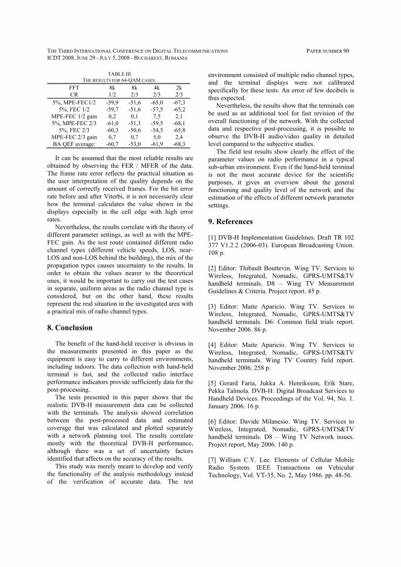
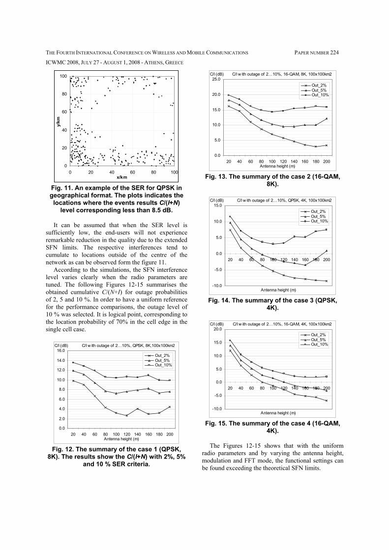
Fig. 11. An example of the SER for QPSK in geographical format. The plots indicates the

locations where the events results C/(I+N) level corresponding less than 8.5 dB.

It can be assumed that when the SER level is

sufficiently low, the end-users will not experience remarkable reduction in the quality due to the extended SFN limits. The respective interferences tend to cumulate to locations outside of the centre of the network as can be observed form the figure 11.

According to the simulations, the SFN interference level varies clearly when the radio parameters are tuned. The following Figures 12-15 summarises the obtained cumulative C/(N+I) for outage probabilities of 2, 5 and 10 %. In order to have a uniform reference for the performance comparisons, the outage level of 10 % was selected. It is logical point, corresponding to the location probability of 70% in the cell edge in the single cell case.

C/I w ith outage of 2…10%, QPSK, 8K,100x100km2

0.0

2.0

4.0

6.0

8.0

10.0

12.0

14.0

16.0

20 40 60 80 100 120 140 160 180 200Antenna height (m)

C/I (dB)

Out_2%Out_5%Out_10%

Fig. 12. The summary of the case 1 (QPSK,

8K). The results show the C/(I+N) with 2%, 5% and 10 % SER criteria.

C/I w ith outage of 2…10%, 16-QAM, 8K, 100x100km2

0.0

5.0

10.0

15.0

20.0

25.0

20 40 60 80 100 120 140 160 180 200Antenna height (m)

C/I (dB)

Out_2%Out_5%Out_10%

Fig. 13. The summary of the case 2 (16-QAM,

8K).

C/I w ith outage of 2…10%, QPSK, 4K, 100x100km2

-10.0

-5.0

0.0

5.0

10.0

15.0

20 40 60 80 100 120 140 160 180 200

Antenna height (m)

C/I (dB)

Out_2%Out_5%Out_10%

Fig. 14. The summary of the case 3 (QPSK,

4K).


-10.0

-5.0

0.0

5.0

10.0

15.0

20.0

20 40 60 80 100 120 140 160 180 200

Antenna height (m)

C/I (dB)

Out_2%Out_5%Out_10%

Fig. 15. The summary of the case 4 (16-QAM,

4K). The Figures 12-15 shows that with the uniform

radio parameters and by varying the antenna height, modulation and FFT mode, the functional settings can be found exceeding the theoretical SFN limits.



The analysis shows that the 8K mode provides with sufficiently low SFN interferences for both QPSK and 16-QAM when GI of ¼ is used. For the QPSK, the minimum required C/(N+I) requirement of 8.5 dB with the outage probability of 10 % is achieved with all the antenna heights of 20…200m . If the mode is changed to 4K, the respective antenna height should be lowered down to 35 m.

16-QAM provides with smaller cell sizes and higher capacity compared to the more robust QPSK cases. The effect of FFT mode can be seen clearly also in this case. For the 16-QAM and 8K, and with the minimum C/(N+I) requirement of 14.5 dB for this specific case, there seem to be no limits for the antenna height as the SFN interference limits are considered. If the mode of this case is switched to 4K, the antenna should be lowered down to 30 m in order to still fulfil the maximum of 10 % outage criteria.

The following Figure 16 summarises the previously presented cases presenting the outage percentage of different modes in function of transmitter antenna height. As previously, 8.5 dB C/(N+I) limit was used for QPSK and 14.5 % for 16-QAM modulation.

Outage-% for antenna heights 20...200m

0.0

5.0

10.0

15.0

20.0

25.0

30.0

35.0

40.0

20 40 60 80 100 120 140 160 180 200Antenna height (m)

Out

age

(%)

Outage%_QPSK,8KOutage%_16-QAM ,8KOutage%_QPSK,4KOutage%_16-QAM ,4K

Fig. 16. The summary of the simulations, showing the outage-% in function of the

transmitter antenna height. The 60 dBm EIRP that was used in the simulations

represents relatively low power class for DVB-H. The higher power level raises the SER level accordingly. For the mid and high power sites the optimal setting depends thus even more on the combination of the power level and antenna height. According to these results, it is clear that the FFT mode 8K is the only reasonable option when the SER should be kept in acceptable level in over-sized SFN areas. According to the results, the over-sized SFN network could be planned using initially QPSK, FFT 8K and GI of ¼ providing large coverage areas but lowest capacity. On

the other hand, when the capacity requirement increases, the switching to the 16-QAM modulation is the most logical solution.

In practice, the SER level can be further decreased by minimising the propagation of the interfering components. This can be done e.g. by adjusting the transmitter antenna down-tilting and using narrow vertical beam widths, producing thus the coverage area of the carrier and interference as close to each others as possible. Also the natural obstacles of the environment can be used efficiently for limiting the interferences far away outside the cell range.

6. Conclusions

The controlled extension of the SFN limit might be

interesting option for the DVB-H operator. The simulation method and results presented in this paper shows logical behaviour of the SFN error rate when varying the essential radio parameters. The results also show that the optimal setting can be obtained using the respective simulation method. As expected, the 8K mode is the most robust when extending the SFN whilst 4K limits the site antenna height considerably. 16-QAM provides suitable performance for the extension, but according to the results, even QPSK is not useless in SFN extension when selecting the parameters correctly.

7. References

[1] DVB-H Implementation Guidelines. Draft TR 102 377 V1.2.2 (2006-03). European Broadcasting Union. 108 p. [2] Jukka Henriksson. DVB-H standard, principles and services. HUT seminar T-111.590. Helsinki, 24 Feb 2005. Presentation material. 53 p. [3] Editor: Thibault Bouttevin. Wing TV. Services to Wireless, Integrated, Nomadic, GPRS-UMTS&TV handheld terminals. D8 – Wing TV Measurement Guidelines & Criteria. Project report. 45 p. [4] Gerard Faria, Jukka A. Henriksson, Erik Stare, Pekka Talmola. DVB-H: Digital Broadcast Services to Handheld Devices. IEEE 2006. 16 p. [5] William C.Y. Lee. Elements of Cellular Mobile Radio System. IEEE Transactions on Vehicular Technology, Vol. VT-35, No. 2, May 1986. pp. 48-56.

IV

Publication IV

“The SFN gain in non-interfered and interfered DVB-H networks”

The paper shows a method for the dimensioning of the DVB-H network’s SFN gain in non-interfering case (inside the allowed SFN limits) as well as in over-sized SFN network that causes interferences. A simulator has been designed for the investigation. A respective simulation is carried out for the most relevant parameter settings and the optimal point of the balance between the SFN gain and SFN error levels has been identified for these case examples.

The Fourth International Conference on Wireless and Mobile Communications

ICWMC 2008

July 27 - August 1, 2008 - Athens, Greece





The SFN gain in non-interfered and interfered DVB-H networks


[email protected]

Abstract

The Single Frequency Network mode (SFN) is one

of the benefits of DVB-H network. In addition to the possibility to use only one frequency in given area, the reception of the same contents via two or more radio paths provides with SFN gain which enhances the quality of service whenever the respective sites are located inside the SFN limits. If the same frequency is used outside the theoretical SFN area, the sites that exceed the relative guard distance converts as interfering sources. This paper describes a simulation method for the investigation of the SFN gain in non-interfered network as well as in the environment with SFN interferences. Also simulation results and analysis with the most logical network parameter set is presented. 1. Introduction

The benefit of Single Frequency Network (SFN) compared to the Multi Frequency Network (MFN) is the possibility to achieve additional signal levels in the coverage area of DVB-H. The level of SFN gain depends on the number of the useful carriers.

The situation changes when the SFN limit is exceeded, i.e. if the maximum diameter of some of the sites is longer than the maximum guard distance of the SFN area. The respective leg of these sites causes interference whenever the difference between the arriving signals exceeds the SFN guard interval.

The paper presents a method for obtaining the value of SFN gain and SER via simulations, by varying the most essential radio parameters. In addition, a set of results for selected cases are shown in order to obtain an optimal balance between SFN gain and the SER

2. Theory of the SFN limits

According to [1], the combination of GI (Guard

Interval) and FFT mode gives the maximum delay that

the DVB-H terminal can handle in order to receive correctly the multi-path components of the signals. The Table 1 summarises the values and the respective SFN distances.

The FFT size has impact on the maximum velocity

of the terminal, and the GI affects on both the maximum velocity of the terminal as well as on the capacity of the radio interface. In these simulations, if the velocity and capacity are not considered, the following parameter combinations results the same C/N and C/(N+I) performance due to their same requirement for the safety distances:

• FFT 8K, GI 1/4: unique case • FFT 8K, GI 1/8: same as FFT 4K, GI 1/4 • FFT 8K, GI 1/16: same as FFT 4K, GI 1/8 and

FFT 2K, GI 1/4 • FFT 8K, GI 1/32: same as FFT 4K, GI 1/16 and

FFT 2K, GI 1/8 • FFT 4K, GI 1/32: same as FFT 2K, GI 1/16 • FFT 2K, GI 1/32: unique case

When the distance between the extreme transmitter sites is less than the SFN determines, the difference of the delays between the signals from different sites is always within the allowed margin. On the other hand, if the distance is greater, the sites interferes, depending if the relative arriving distance of the respective sites is greater than the safety margin shown in Table 1. The received signal is still functional if the total C/(N+I) is at least in the same level as the original minimum required C/N for the respective parameter set.

Table 1. The guard interval lengths and respective SFN distances.

GI FFT = 2K FFT = 4K FFT = 8K

µs km µs km µs km 1/4 56 16.8 112 33.6 224 67.0 1/8 28 8.4 56 16.8 112 33.6 1/16 14 4.2 28 8.4 56 16.8 1/32 7 2.1 14 4.2 28 8.4



The required C/N depends on the values of code rate (CR), MPE-FEC rate (multi protocol encapsulator, forward error correction) and modulation scheme. The minimum C/N requirement for some of the most common parameter setting can be seen in Table 2. [1]

For the carrier and interfering signal, the total level

of C/(N+I) is the squared sum of the C/N and I/N components in absolute powers (watt), thermal noise floor and terminal noise factor being the reference.

3. Methodology for SFN simulations

The SFN performance simulator is based on the

hexagonal cells. The Figure 1 presents the idea of the cell distribution.

TX(x,y)

TX(x,2)

TX(1,1) TX(2,1) TX(3,1) TX(x,1)

TX(x-1,2)TX(2,2)TX(1,2)

TX(1,3) TX(2,3) TX(3,3) TX(x,3)

TX(x-1,y)TX(2,y)TX(1,y)

Fig. 1. The active transmitter sites are selected

from the 2-dimensional cell matrix. A uniform parameter set is used for each cell site

including the transmitter power level and antenna height. This yields the same radius for each cell per simulation case. The coordinates of each site depends on the uniformly calculated cell radius.

Investigating the Figures 1-2 and the hexagonal model behaviour, the x-coordinates can be obtained in the following way depending if the row number for y coordinates is odd or even.

30deg

r30deg

x/2

x

y

x/2

30deg

Fig. 2. The geometrical characteristics of the

hexagonal model used in the simulator. The distance between two sites in x-axis is:

( ) rrx 866.0230cos2 ⋅=°= (1) The common inter-site distance in y-axis is:

( )( ) 3

230tan30cos rry =°°

= (2)

In odd row case, the formula for the x-coordinates

of the site m is thus the following:

( ) rmrmx odd 732.11)( ⋅−+= (3) In the formula, m represents the number of the cell

in x-axis. In the same manner, the formula for x-coordinates can be created in the following way:

( ) ( ) rmrrmx even 732.11732.121

⋅−++= (4)

For the y-coordinates, the formula is the following:

( ) ( ) rnrny321 ⋅−+= (5)

The simulations can be carried out for different cell

layouts. Symmetrical reuse pattern concept was selected for the simulations presented in this paper. The most meaningful reuse pattern size K can be obtained with the following Formula [5]:

kllkK −−= 2)( (6)

The variables k and l are positive integers with

minimum value of 0. In the simulations, the reuse pattern sizes of 1, 3, 4, 7, 9, 12, 16, 19 and 21 was used for the carrier and interference distribution in both non-interfering and interfering networks (i.e. SER either exists or not depending on the size of the SFN

Table 2. The minimum C/N (including antenna loss) for the selected parameter settings.

Parameters C/N (dB)





area). In this way, the lower values of K provides with the non-interfering SFN network until a limit that depends on the GI and FFT size parameters.

The single cell (K=1) is considered as a reference in all of the cases. The fixed parameter set was the following:

• Transmitter power: 60 dBm • Transmitter antenna height: 60 m • Receiver antenna height: 1.5 m • Long-term fading with normal distribution and

standard deviation of 5.5 dB • Area coverage probability in the cell edge: 70% • Receiver noise figure: 5 dB • Bandwidth: 8 MHz • Frequency: 700 MHz

For the used bandwidth, the combined noise floor and noise figure yields -100.2 dBm as a reference for calculating the level of C and I. The path loss was calculated with Okumura-Hata prediction model for small and medium sized city. The 70 % area coverage probability corresponds with 10% outage probability in the single cell area. These settings result a reference C/N of 8.5 dB for QPSK and 14.5 dB for 16-QAM. The value is the minimum acceptable C/N, or in case of interferences, C/(N+I) value that is needed for the successful reception of the signal.

The Figure 3 presents the symmetrical reuse pattern sizes that were selected for the simulations. The grey hexagonal cells means that the coordinates has been taken into account calculating the order number of the sites (formulas 3-5), but the respective transmitter has been switched off in order to form the correct reuse pattern. The Figure 4 shows an example of the network setup and locations for the QPSK and K=7.

Fig. 3. The reuse patterns, K=1, 3, 4, 7, 9, 12,

16, 19 and 21.

Network layout for K=7

-10

0

10

20

30

40

0 10 20 30 40 50

x (km)

y (k

m)

Fig. 4. An example of the QPSK network, K=7.

The Figure 5 shows an example of the C/N

distribution with the parameter values of K=7, GI=1/4, and FFT=8K. According to the C/I link analysis, the case presented in Figure 5 is free of SFN interferences.

Fig. 5. An example of the simulated case with

QPSK and K=7. The actual simulation results for C/N, or in case of

the interferences, for C(/N+I), is done in such way that only the terminal locations inside the calculated cell areas is taken into account. If the MS is found outside of the network area (the circles) in some simulation round, the result is simply rejected.

The Figure 6 shows the principle of the filtered simulation. As the terminal is always inside the coverage area of at least one cell, it gives the most accurate estimation of the SFN gain with different parameter values. Furthermore, the method provides a reliable means to locate the MS inside the network area according to the uniform distribution.



Fig. 6. The results in filtered area. This

principle is used in the simulations. The network was dimensioned in such way that the

area location probability is 70% in the cell edge. The dimensioning can be made by taking into account the characteristics of long-term fading. The Figure 7 shows a snap-shot type example in filtered area with the C/N values resulting less than 8.5 dB, i.e. the limit for the respective parameter settings of QPSK cases.

Fig. 7. An example of the distribution of the simulation results that yields C/N < 8.5 dB. As a verification of the geographical interference

class, a study that can be called a “C/I-link analysis” was carried out. It is a method to revise all the combinations (hash) of the distances between each pair of sites (TX1-TX2, TX1-TX3, TX2-TX1, TX2-TX3 etc.) marking the link useful (C) if the guard distance between the respective sites is less than the maximum allowed SFN diameter (DSFN). If the link is longer, it is marked as a potential source of interference (I).

The interference link proportion can be obtained for each case by calculating the potential interference links over the total links. It gives a rough idea about the “severity” of the exceeding of the SFN limit, with a value range of 0-100% (from non-interfering network up to interfered network where all the transmitters are a potential source of interference).

4. Results

The Tables 3 and 4 summarises the C/I link analysis

for the different reuse pattern sizes and for FFT and GI with the selected radio parameter values.

The C/I link analysis shows that in case of large

network (21 cells in the SFN area), the only reasonable parameter set for the QPSK modulation seems to be FFT=8K and GI=1/4. This is due to the fact that QPSK provides with the largest cell sizes (with the investigated parameter set the r=7.5 km). The cell size of the investigated 16-QAM case is smaller (r=5.0 km)

Table 4. The C/I link analysis for 16-QAM. Reuse pattern size (K)

FFT,GI 3 4 7 9 12 16 19 21

8K, 1/4 0 0 0 0 0 0 0 0

4K, 1/4 0 0 0 0 0 0.8 1.8 5.7

2K, 1/4 0 0 14.3 30.6 42.4 49.1 57.9 61.9

8K, 1/8 0 0 0 0 0 0.8 1.8 5.7

4K, 1/8 0 0 14.3 30.6 42.4 49.1 57.9 61.9

2K, 1/8 100 100 100 100 100 100 100 100

8K, 1/16 0 0 14.3 30.6 42.4 49.1 57.9 61.9

4K, 1/16 100 100 100 100 100 100 100 100

2K, 1/16 100 100 100 100 100 100 100 100

8K, 1/32 100 100 100 100 100 100 100 100

4K, 1/32 100 100 100 100 100 100 100 100

2K, 1/32 100 100 100 100 100 100 100 100

Table 3. The C/I link analysis for QPSK cases. Reuse pattern size (K)

FFT,GI 3 4 7 9 12 16 19 21

8K, 1/4 0 0 0 0 0 0 0 0.5

4K, 1/4 0 0 0 11.1 24.2 36.7 42.1 47.1

2K, 1/4 0 16.7 42.9 55.6 65.2 72.5 75.4 78.1

8K, 1/8 0 0 0 11.1 24.2 36.7 42.1 47.1

4K, 1/8 0 16.7 42.9 55.6 65.2 72.5 75.4 78.1

2K, 1/8 100 100 100 100 100 100 100 100

8K, 1/16 0 16.7 42.9 55.6 65.2 72.5 75.4 78.1

4K, 1/16 100 100 100 100 100 100 100 100

2K, 1/16 100 100 100 100 100 100 100 100

8K, 1/32 100 100 100 100 100 100 100 100

4K, 1/32 100 100 100 100 100 100 100 100

2K, 1/32 100 100 100 100 100 100 100 100



which provides the use of the parameter set of (FFT = 8K, GI = 1/4), (FFT = 4K, GI = 1/4) and (FFT = 8K, GI = 1/8). The interference distance rinterference=13.5 km is the same in all the cases as the interference affects until it reaches the reference level (the sum of noise floor and terminal noise figure).

The C/I link investigation gives thus a rough idea about the most feasible parameter settings. In order to obtain the information about the complete performance of DVB-H, the combination of the SFN gain and SER level should be investigated.

The Figures 8 and 9 shows examples of two extreme cases of the simulations, i.e. PDF of non-interfered and completely interfered situation. As for all of the simulation cases, a total of 60,000 simulation rounds were performed. The figures shows the PDF, i.e. occurred amount of samples per C/N and C/I in scale of 0-50 dB, with 0.1 dB resolution.

PDF, C/N, QPSK, K=7, FFT=8K, GI=1/4

1

10

100

1000

0 5 10 15 20 25 30 35 40 45 50C/N (dB)

# of

sam

ples

C distribution

I distribution

Fig. 8. An example of the C/N distribution in

non-interfered SFN network.

PDF, C/(N+I), 16-QAM, K=7, FFT=2K, GI=1/32

1

10

100

1000

0 5 10 15 20 25 30 35 40 45 50C/(N+I) (dB)

# of

sam

ples

C distribution

I distribution

Fig. 9. An example of C/N and I/N in interfered

case.

The PDF gives a visual indication about the general quality of the network. Nevertheless, in order to obtain the exact values of the performance indicators, a cumulative presentation is needed. The following Figure 10 shows an example of the CDF in the non-interfering QPSK network with the reuse pattern size as a variable.

CDF, C/N, QPSK, K=1...21, FFT=8k, GI=1/4

00.10.20.30.40.50.60.70.80.9

1

0 5 10 15 20 25 30 35 40 45 50C/N (dB)

1 34 79 1216 1921

Fig. 10. The CDF of C/N in non-interfered network for reuse pattern sizes of 1-21.

The Figure 11 shows an amplified view to the

breaking point, i.e. the 10% outage probability criteria.

CDF

0

0.1

0.2

0.3

0.4

0 5 10 15 20C/(N+I) (dB)

K=K=K=K=K=K=12

K=16K=19K=21

Fig. 11. An amplified view of the example of

the simulation results for QPSK network As can be seen form the Figure 11, the single cell

(K=1) results a minimum of 8.5 dB for the 10 % outage probability, i.e. for the area location probability of 90% in the whole cell area which corresponds to the 70% area location probability in the cell edge. The cell is thus correctly dimensioned for the simulations.



In order to find the respective SFN gain level, the comparison with single cell and other reuse pattern sizes was made in the 10% outage point. The Figures 12-13 shows the simulation results for the reuse pattern sizes 1-21.

SFN gain, QPSK

-15.0

-10.0

-5.0

0.0

5.0

1 3 4 7 9 12 16 19 21

K

SFN

gai

n (d

B)

GI1/4,8KGI1/4,4KGI1/4,2KGI1/8,2KGI1/16,2KGI1/32,2K

Fig. 12. The SFN gain levels for QPSK cases,

with the reuse pattern sizes of 1-21.

SFN gain, 16-QAM

-20.0

-15.0

-10.0

-5.0

0.0

5.0

1 3 4 7 9 12 16 19 21

K

SFN

gai

n (d

B)


Fig. 13. The SFN gain levels for 16-QAM cases,

with the reuse pattern sizes of 1-21. The simulation results show the level of SFN gain.

The reference case (FFT 8K and GI ¼) results the maximum gain for the reuse pattern sizes of K=1-21 for both QPSK and 16-QAM and provides a non-interfering network. In addition, the parameter set of (FFT = 4K, GI = 1/4) and (FFT = 8K, GI = 1/8) results a network where SFN errors can be compensated with the SFN gain.

According to the results shown in Figure 12, the QPSK case could provide SFN gain of 3-4 dB in non-interfering network. It is interesting to note that in the interfering cases, also the parameter set of (GI = ¼, FFT = 4K corresponding FFT = 8K, GI = 1/8) results

positive SFN gain even with the interference present for all the reuse pattern cases up to 21. Also the parameter set of (GI = ¼, FFT = 2K, corresponding FFT = 8K, GI = 1/16 and FFT = 4K, GI = 1/8) provides an adequate quality level until reuse pattern of 16 although the error level (SER) increases.

According to the Figure 13, the 16-QAM gives equal SFN gain, resulting about 3-4 dB in non-interfering network. For the (FFT = 4K, GI = ¼) and the corresponding parameter set of (FFT = 8K, GI = 1/8), the SFN gain is higher than the SER even with higher reuse pattern sizes compared to QPSK, because the 16-QAM cell size is smaller.

As can be seen from the Figures 12-13 and from the C/I link analysis of Tables 3-4, the rest of the cases are useless with the selected parameter set.

5. Conclusions

The simulation method presented in this paper can

be used in the in-depth optimisation of the DVB-H. The results show the SFN gain in non-interfered as well as in the over-sized and interfered SFN network.

Especially in the interfered SFN network, the correct selection of the radio parameters is essential. The results show that the interference level can be compensated with the SFN gain, and sufficiently good quality of service (e.g. the level that would be achieved by using only one site without SFN gain) can thus be obtained by selecting correctly the radio parameters.

6. References [1] DVB-H Implementation Guidelines. Draft TR 102 377 V1.2.2 (2006-03). European Broadcasting Union. 108 p. [2] Jukka Henriksson. DVB-H standard, principles and services. HUT seminar T-111.590. Helsinki, 24 Feb 2005. Presentation material. 53 p. [3] Editor: Thibault Bouttevin. Wing TV. Services to Wireless, Integrated, Nomadic, GPRS-UMTS&TV handheld terminals. D8 – Wing TV Measurement Guidelines & Criteria. Project report. 45 p. [4] Gerard Faria, Jukka A. Henriksson, Erik Stare, Pekka Talmola. DVB-H: Digital Broadcast Services to Handheld Devices. IEEE 2006. 16 p. [5] William C.Y. Lee. Elements of Cellular Mobile Radio System. IEEE Transactions on Vehicular Technology, Vol. VT-35, No. 2, May 1986. pp. 48-56.

V

Publication V

“DVB-H coverage estimation in highly populated urban area”

The paper compares the DVB-H coverage area estimations via the theoretical Okumura-Hata model and typical radio network planning program that is based on the Okumura-Hata propagation model with respective correction factors. The investigation shows the coverage estimations in the urban area of Mexico City.

58th Annual IEEE Broadcast Symposium

15-17 October 2008, Alexandria, VA, USA



Abstract The methodology for the sufficiently accurate DVB-H coverage estimation is one of the most important topics in the network planning of the system. The final coverage area depends on the planned capacity, i.e. the bit stream per channel, as well as the number of the channels. Also the surrounding geographical area has a big impact on the coverage, as well as the antenna height. This paper shows a case analysis about the coverage estimation as a basis for the initial radio network planning in large urban environment. The study was carried out for Mexico City, which is one of the most populated areas in the world.

Keywords DVB-H, radio network planning.

INTRODUCTION The coverage area of a single DVB-H transmitter site depends on the provided capacity and thus on the radio parameters that provides the required bit pipe. Logically, higher total capacity demand in the given band width results smaller cell sizes.

The environment has a big impact on the radio wave propagation. According to the Okumura-Hata [8] prediction model, the dense urban area attenuates the signal considerably compared to the other environment types.

This paper shows an example of the coverage planning in Mexico City, which is considered as one of the largest urban and dense urban environments. Despite of the challenges of the presented environment type, the definite advantage of DVB-H can be seen most clearly in this case as big amount of potential customers can be served in reduced area. In Mexico City alone, the estimated total population is about 20-25 million from which the number of the potential customers can be estimated to be considerable.

The study presented in this paper compares the accuracy and usability of the basic Okumura-Hata model and more in-depth coverage planning tool with respective terrain height and area type information included.

THE PLANNED ENVIRONMENT Mexico City is situated in 1.4 miles (2.2 km) of height from the sea level, and it is surrounded by the mountains with about 1.9 miles (3 km) of height compared to the sea level.

Figure 1 shows an overview of the city. As can be observed, the area consists of urban buildings in large area.

Figure 1. An overview of Mexico City, near the center

area. The city is in general tightly built and large in size.

The following Figure 2 shows the area cluster type of Mexico City. As can be seen, the dense urban and urban type is very large with the respective cluster type proportion of roughly 420 square miles (1000 km2).

urban

dense urban

forest

open

residential

4 8 12 16 20km 4 8 12 16 20km

Figure 2. The area type, i.e. cluster map of Mexico City. This map shows the area of about 30 × 30 miles (50 × 50

km) from which half is urban and dense urban area.

DVB-H Coverage Estimation in Highly Populated Urban Area

Jyrki T.J. Penttinen Nokia Siemens Networks, Spain

[email protected]

THEORETICAL COVERAGE ESTIMATION The assumption for the analysis was to use 16-QAM modulation, which provides about two times more channel capacity compared to QPSK. On the other hand, the link budget of 16-QAM produces about 6-7 dB smaller coverage than QPSK.

For the sufficiently robust channel coding and error recovery, the Code Rate (CR) of ½ and MPE-FEC rate of ¾ was selected. With 16-QAM modulation and 17.5 dB C/N requirement, this results a total channel capacity of 6.2 Mb/s. Using the basic SFN network, this combination would be possible to use e.g. for 1 ESG (electrical service guide, about 200–300 kb/s) and for 10–12 high quality audio-video channels of about 450 kb/s each, or for about 20 good quality A/V channels of about 250 kb/s each.

In the initial phase of the planning, an Okumura-Hata based rough estimation about the needed amount of sites can be carried out using the respective area correction. For the estimation of the cell size (radius), a link budget is a proper tool. In this specific case, the link budget shown in Table 1 can be created.

Table 1. An example of the DVB-H link budget.

General parametersFrequency f 680.0 MHzNoise floor for 6 MHz bandwidth P n -106.4 dBmRX noise figure F 5.2 dBTXTransmitter output power P TX 2400.0 WTransmitter output power P TX 63.8 dBmCable and connector loss L cc 3.0 dBPower splitter loss L ps 3.0 dBAntenna gain G TX 13.1 dBiAntenna gain G TX 11.0 dBdEff. Isotropic radiating power EIRP 70.9 dBm

EIRP 12308.7 WEff. Radiating power ERP 68.8 dBm

ERP 7502.6 WRXMin C/N for the used mode (C/N) min 17.5 dBSensitivity P RXmin -83.7 dBmAntenna gain, isotropic ref G RX -7.3 dBiAntenna gain, 1/2 wavelength dipole G RX -5.2 dBdIsotropic power P i -76.4 dBmLocation variation for 95% area prob L lv 5.3 dBBuilding loss L b 14.0 dBGSM filter loss L GSM 0.0 dBMin required received power outdoors P min(out) -71.1 dBmMin required received power indoors P min(in) -57.1 dBm

Min required field strength outdoors E min(out) 62.8 dBuV/mMin required field strength indoors E min(in) 76.8 dBuV/mMaximum path loss, outdoors L pl(out) 142.0 dBMaximum path loss, indoors L pl(in) 128.0 dB

According to the link budget, the outdoor reception of this specific case with 2,400 W transmitter yields a successful

reception when the radio path loss is equal or less than 142.0 dB.

The Okumura-Hata model [8] can be applied in order to obtain the cell radius (unit in kilometers) in large city type.

[ ] )lg()lg(55.69.44

)()lg(82.13)lg(16.2655.69)(

dh

hahfdBL

BS

MSBS i

−+

−−+=

( )[ ]

( )[ ] MHzhha

MHzhha

MSLCMS

MSLCMS

400f ,97.475.11lg2.3)(

200f ,10.154.1lg29.8)(

22

21

≥−=

≤−=

[ ]

−

−−+−

= )lg(55.69.44

)()lg(82.13)lg(16.2655.69)(

10 BS

iMSBS

h

hahfdBL

d The following Figure 3 presents the estimated cell range

calculated with the large city model and by varying the transmitter antenna height and power level.

Cell radius

0.0

2.0

4.0

6.0

8.0

10.0

12.0

14.020 40 60 80 100

120

140

160

180

200

Antenna height (m)

d (k

m)

P=1500WP=2400WP=3400WP=4700W

Figure 3. The cell range calculated with the Okumura-Hata model for the large city, varying the transmitter

power levels. According to the Figure 3, it is clear that higher the

antenna is located and higher the transmitter power is, lower is the transmitter site number. In practice, though, it is not always possible to obtain the site locations and antenna heights in the technically best locations. The access for already existing towers might be limited as well as the available heights in the towers, and rooftops might be challenging to obtain. In many cases, the antenna height is limited to 65–100 feet (20–30 m). In some cases, it could be possible to obtain a higher antenna location in broadcast tower near the city center, or even better, in skyscraper’s rooftop in the downtown area.

On the other hand, the transmitter type is important to select correctly. In case of high-power transmitter type, the respective power consumption increases. It can be estimated

that the power consumption might be about 6 times the produced power level fed to the antenna cable. Also the complexity rises among the higher power levels, and e.g. liquid cooling is needed instead of air cooling, affecting on the maintenance. These might be limitations for the highest power classes when selecting the optimal power levels.

In this analysis, a 2,400 W transmitter type was selected due to the above mentioned reasons. According to the Figure 3, it provides a cell radius of 1.9–2.5 miles (3–4 km) with the transmitter antenna installed to 65–130 feet (20–40 m) of height. As a comparison, the antenna height of 330 feet (100 m) provides about 4.4 miles (7 km) cell radius, and 660 feet (200 m) antenna yields about 6.2–6.8 miles (10–11 km) radius. If possible to install, one or two high antenna locations would provide a good basic coverage in the city area whilst the sites with lower antenna heights fills the rest of the area.

If only the urban and dense urban areas are to be covered, the following theoretical coverage map can be created by selecting 2 sites with antenna height of 660 feet (200 m) and cell radius of 6.8 miles (11 km), and the rest of the sites could use antenna heights of 100 feet (30 m) which provides a cell radius of about 2.2 miles (3.5 km). The map represents the Okumura-Hata estimated coverage for the outdoor assuming the sites can be selected without restrictions.

4 8 12 16 20km 4 8 12 16 20km

Figure 4. Theoretical coverage plan when using

Okumura-Hata model for the cell radius estimation. The drawback of the above presented coverage plan is

that the prediction is inaccurate depending on the actual terrain type. Nevertheless, it gives an idea about the rough cell number. In any case, this analysis shows the importance of the antenna height as with only two high antenna locations, it looks possible to cover about half of the given area whilst the low antenna locations results a need of about 15 sites.

PLANNING TOOL ANALYSIS In order to compare the theoretical Okumura-Hata approach with the more realistic methods, Nokia NetAct Planner was used as a basis for more in-depth analysis of the coverage planning. The tool consists of the digital maps of Mexico City, with respective clutter data. A total of 7 sites were selected for the analysis based on the practical site considerations, i.e. the selected sites could possibly be real candidates with realistic antenna heights.

The NetAct consists of several propagation models. Extended Okumura-Hata prediction model with respective digital cluster maps was used in the analysis. The initial parameter tuning for the DVB-H plan was made based on the estimated local clutter attenuation factors. The final clutter values and other propagation model parameterization for the estimated coverage area should be adjusted by carrying out field tests as each area type differs from the others.

The coverage map was plotted for outdoor and indoor environments based on the previously used DVB-H link budget, taking into account the relevant parameters (bandwidth, modulation scheme, code rate, MPE-FEC rate and receiver antenna gain). The same 2,400 W transmitter type was used in all the sites like in previous analysis, with EIRP of about 69–71 dBm, depending on the site configuration, i.e. cable lengths and losses. In this analysis, 2 or 3 directional antennas with the horizontal beam width of 65 degrees and vertical beam of 27 degrees was used, with respective antenna gain of 13.1 dBi. In some cases of high antenna installations, a slight antenna element down-tilting was used in order to optimize the coverage.

Other essential global parameters for the link budget were: Code rate (CR) ½, MPE-FEC rate ¾, radio channel TU6 (with 30 Hz Doppler), channel bandwidth 6 MHz and 680 MHz operating frequency. The average building penetration loss was estimated to be 14 dB. With the area location probability of 95 %, the link budget yields a minimum requirement of -71.1 dBm for the received power level in this specific case.

The following Table 2 presents the selected sites with the antenna height hant, direction (degrees), down-tilt (DT) and the final EIRP (dBm) values. The EIRP shown in the Table includes the transmitter filter, cable, connector and power splitter loss.

Table 2. The DVB-H site configuration. Site TX P hant deg DT EIRP

Tres Padres 2400 W 60 m 140/220 2/2 70.5 WTC 2400 W 190 m 0/150/240 2/2/2 69.3 Iztapalapa 2400 W 30 m 0/120/240 0/0/0 69.3 Santa Fe 2400 W 20 m 0/120/240 0/0/0 69.5 Tlalpan 2400 W 20 m 330/90 0/0 71.3 Vallejo 2400 W 30 m 0/120/240 0/0/0 69.3 Azteca 2400 W 30 m 120/240 0/0 71.1

The coverage plots indicates the functional areas for 16-QAM in outdoor and indoor environments. As a reference, also QPSK outdoor coverage is presented, with the colors shown in the following Figure 5. In the following coverage maps, the raster size is 3.1 × 3.1 miles (5 × 5 km).

Outdoor 16-QAM coverage Indoor

16-QAM coverage

Outdoor QPSK coverage

Figure 5. The meaning of the plotted colors.

Two possibilities were identified for the high antenna

installation; the “WTC” (skyscraper) and “Tres Padres” (mountain). The WTC site (with 623 feet / 190 m antenna height) provides a good basic coverage with more than 6.2 miles / 10 km radius (NetAct) in main beam, or 5.5 miles / 8.7 km (Okumura-Hata). It is worth noting, though, that the used prediction model does not take into account the variations of the obstacles like detailed building heights, so there might be holes in the presented map especially in the street canyons.

EIRP: 69.3 dBmAnt: 0/150/240 deg, 190 mDowntilt: 2/2/2 deg

Figure 5. “WTC” site.

The other high antenna site, “Tres Padres”, was planned

with 2 sectors pointing south-east and south-west in high mountain tower (about 1.9 miles / 3 km from sea level, whilst the average value of the city area is about 1.4 miles / 2.2 km). It provides a large basic coverage. Depending on the obstacles in LOS and observed direction, the outdoor coverage varies within 3.1–15.5 miles / 5–25 km of radius.

Okumura-Hata is not valid in this case as the radius is more than 20 km, but e.g. ITU-R P.1546 model yields 9.4 miles / 15 km with the parameter values of this example which is in align with the estimation shown in the Figure 6.

EIRP: 70.5 dBmAnt: 140/220 deg, ~3km above sea levelDowntilt: 2/2/2 deg

Figure 6. “Tres padres” site.

“Tlalpan” was planned with 2 sectors in a tower (antenna

in 65 feet / 20 m), which provides only local coverage. The outdoor coverage is about 1.9 miles / 3 km (1.8 miles / 2.8 km via Okumura-Hata) of radius in the main beam of the antennas.

EIRP: 71.3 dBmAnt: 330/90 deg, 20 mDowntilt: 0/0 deg

Figure 7. “Tlalpan” site

“Iztalapa” was planned with 3 sectors in a tower (antenna

height 100 feet / 30 m). It provides only a local coverage. Depending on the obstacles in LOS, the outdoor coverage is

about 2.5 miles / 4 km (1.9 miles / 3.1 km via Okumura-Hata) of radius in main beams.


Figure 8. “Iztalapa” site.

“Vallejo” contains 3 sectors (antenna height 100 feet / 30

m). It provides a local coverage due to the low antenna height, but nevertheless, it increases the indoor coverage in “Tres padres” sector. Depending on the obstacles in main beams, the outdoor coverage is about 2.1 miles / 4 km (1.9 miles / 3.1 km via Okumura-Hata) of radius.


Figure 9. “Vallejo” site.

“Santa Fe” with 3 sectors in a tower (antenna height 65

feet / 20 m) provides relatively small local coverage for the low antenna height and non-uniform terrain. Depending on the obstacles in man beams, the outdoor coverage is about

1.6 miles / 2.5 km (1.6 miles / 2.5 km via Okumura-Hata) of radius. The challenge of this site is the variations of the mountain heights nearby.


Figure 10. “Santa Fe” site.

“Azteca” with 2 sectors (antenna height 65 feet / 20 m)

provides relatively good local coverage in the directions without obstacles. Depending on the obstacles, the outdoor coverage varies in range of 1.9–6.2 miles / 3–10 km (2.2 miles / 3.6 km via Okumura-Hata) of radius.

EIRP: 71.1 dBmAnt: 120/240 deg, 30 mDowntilt: 0/0/0 deg

Figure 11. “Azteca” site.

The following Figure 12 presents the complete network

coverage with the 7 sites. The plot shows the network coverage with 16-QAM and 95 % area location probability, code rate of ½ and MPE-FEC of 2/3.

Figure 12. The complete network coverage prediction.

RESULTS The cell size estimation obtained by calculating with pure Okumura-Hata prediction model has relatively good average correlation with the results that can be obtained with NetAct Planner when the general limits of the models are taken into account.

The results of the NetAct Planner shows that the used prediction takes well into account the terrain heights and cluster types, which would be challenging to do with using only theoretical Okumura-Hata approach. When sufficiently good line of sight is found in the planned sector, the useful cell size may be considerably better that obtained with the use of Okumura-Hata.

The number of identified site number was relatively low in the NetAct analysis. More sites are obviously needed if the same area should be covered as shown in Okumura-Hata analysis in Figure 4. By observing the Figure 12, about 4–6 additional sites might be necessary for the full coverage. Okumura-Hata estimated well the relatively low antenna installation sites, but the model estimated the coverage area of the high WTC site in pessimistic way which affects on the final estimation of the sites.

It is worth noting that especially the indoor coverage in selected areas requires the use of repeater type of solution, e.g. in shopping centers and other centralized locations, where the potential customers are typically using the service.

CONCLUSIONS The results of the case analysis shows that the theoretical Okumura-Hata prediction model with DVB-H link budget gives a good first-hand estimate about the cell sizes and thus about the needed amount of the sites in the planned area. Taking into account the characteristics of the model, this method can be applied especially in the initial phase of the

network planning. Due to the restrictions of the Okumura-Hata ranges as the

antenna height and maximum estimated cell radius are considered, the methodology applies for the relatively decent radiating power levels. When the cell radius exceeds the maximum predictable value of 12.4 miles / 20 km, as the case is for the “Tres Padres” site, the model is not feasible and adjusted models should thus be used. Especially for the high antenna locations, one of the most logical models at the moment is the ITU recommendation P.1546, which is based on the curve mapping and is valid practically for all the environments where DVB-H can be constructed. On the other side, the power levels are limited due to the EMC and human exposure regulation resulting sufficiently small cell ranges in order to be estimated with Okumura-Hata in mayor part of the cases in urban areas.

The advanced planning tool with respective digital maps including the terrain height and correct cluster attenuation information is essential in the detailed network planning. It is also worth noting that the predictions presented in this paper gives indication only about the coverage areas. Especially in the case of Single Frequency Network, the correct balancing of the FFT size and Guard Interval values is important in order to avoid too high level of the possible inter-symbol interferences in large single frequency network areas.

The results shows that the coverage estimation presented in this paper can be used in the first phase of the DVB-H radio network planning for the initial estimation of the transmitter sites. As the clutter types vary in practice, the more detailed prediction estimations with respective model tuning via the field tests are thus needed in the following phases.

REFERENCES [1] Limits of Human Exposure to Radiofrequency Electromagnetic Fields

in the Frequency Range from 3 kHz to 399 GHz. Safety Code 6. Environmental Health Directorate, Health Protection Branch. Publication 99-EHD-237. Minister of Public Works and Government Services, Canada 1999. ISBN 0-662-28032-6. 40 p.

[2] DVB-H Implementation Guidelines. Draft TR 102 377 V1.2.2 (2006-03). European Broadcasting Union. 108 p.

[3] Jukka Henriksson. DVB-H standard, principles and services. HUT seminar T-111.590. Helsinki, 24.2.2005. Presentation material. 53 p

[4] Editor: Thibault Bouttevin. Wing TV. Services to Wireless, Integrated, Nomadic, GPRS-UMTS&TV handheld terminals. D8 – Wing TV Measurement Guidelines & Criteria. Project report. 45 p.

[5] Gerard Faria, Jukka A. Henriksson, Erik Stare, Pekka Talmola. DVB-H: Digital Broadcast Services to Handheld Devices. IEEE 2006. 16 p.

[6] William C.Y. Lee. Elements of Cellular Mobile Radio System. IEEE Transactions on Vehicular Technology, Vol. VT-35, No. 2, May 1986. pp. 48-56.

[7] Myron D. Fanton. Analysis of Antenna Beam-tilt and Broadcast Coverage. ERI Technical Series, Vol 6, April 2006. 3 p.

[8] Masaharu Hata. Empirical Formula for Propagation Loss in Land Mobile Radio Services. IEEE Transactions on Vehicular Technology, Vol. VT-29, No. 3, August 1980. 9 p.

[9] Recommendation ITU-R P.1546-3. Method for point-to-area predictions for terrestrial services in the frequency range 30 MHz to 3000 MHz. 2007. 57 p.

VI

Publication VI

“DVB-H Radiation Aspects”

The paper shows a method to estimate the safety distances for both human exposure and EMC in typical installation environments of the DVB-H antennas.

IEEE International Symposium on Wireless Communication Systems 2008 (ISWCS’08)

21 – 24 October 2008, Reykjavik, Iceland



Abstract—The typical radiating power levels of the DVB-H sites are normally between the values used in mobile and television broadcast networks. It is thus important to take into account accordingly the EMC (Electro Magnetic Compatibility) as well as the human exposure limits in the DVB-H transmission facilities. This paper presents a practical method for estimating the safety limits of human exposure and EMC in different DVB-H installation environments. Furthermore, case studies are presented for the most typical environments.

Index Terms—DVB-H, planning, optimisation, radiation, safety

I. INTRODUCTION HE radiation of the DVB-H transmitter sites can be

assumed to be higher than in mobile networks. As there are normally mobile or broadcast systems installed in the same site as DVB-H, it is essential to dimension the safety distances in order to minimise the risk of inter-system interferences. On the other hand, the human exposure limits must be calculated for both technical installation personnel and for the public.

The DVB-H transmitter site antennas can be located to the telecom or broadcast tower as well as on the rooftop or indoors of the buildings. The power level should be adjusted accordingly in order to avoid any interferences or safety zone extensions. This paper presents the methodology to estimate the safety distances in typical environments.

II. SAFETY ASPECTS The DVB-H radio transmission is defined to the frequency

range of 470-862 MHz (UHF IV and V) with a channel bandwidth of 5, 6, 7 or 8 MHz. The channels can be divided into several sub-channels as the used bit stream is relatively low. DVB-H can also be deployed to VHF III and L bands.

The power level of DVB-H depends on the transmitter manufacturer solutions. Typically, the power amplifiers can produce around 100-9000 W (output power to the feeder), although the maximum power level might be limited to few thousands of watts in practical solutions.

DVB-H radiation is non-ionising like in case of mobile network technologies. The radiation does not thus alter the human cell structure as can happen in ionising systems like x-ray equipment. Nevertheless, a sufficiently high non-ionising radio transmission power can increase the cell temperature.

The radiation in given distance can be estimated with various propagation models. The simplest one giving the maximum values is the far-field attenuation in free space:

( ) ( )fdL log20log2044.32 ++= (1)

The safety distance of the DVB-H antennas must be assured in the deployment of the system. A simple but practical method can be created based on the fact that the antenna is located to the tower or rooftop, and that the most meaningful area to be investigated is found below the antenna.

The DVB-H antenna solution can be based on omni-radiating poles or directional antennas. The Figure 1 shows an example of the far-field horizontal and vertical radiation patterns of the directional antenna used in DVB-H. As can be observed from the Figure, in the practical installation environments, the vertical radiation pattern is the most meaningful when estimating the field strength and safety zones.

0

-3

-10

0

-3

-10

0

-3

-10

0

-3

-10

Fig. 1. Example of the horizontal plane of the antenna radiation pattern. The 3 dB attenuation determinates the beam width. In this specific case, the beam width is about 60 degrees. The second pattern shows an example of the vertical plane of the directional antenna radiation. In this case, the beam width in 3 dB attenuation points is about +/- 14 degrees, i.e. 28 degrees.

In order to obtain the safety limits below the DVB-H antenna, a loss analysis with different angles from the antenna can be done. Having the vertical antenna pattern, respective coordinate system and linear scale for the antenna radiation attenuation as shown in Figure 2, an antenna attenuation table can be created with the scale from 270 to 180 degrees (back lobe) and from 180 to 90 degrees (main beam). 180 degree vertical angle means the point below the antenna. In this specific example, the following Table I can be obtained from the respective antenna data. The 90 degree angle represents the main beam of the antenna with 0 dB loss. Please note the difference with the conventional marking of the angles, as normally 0 degree elevation represents the horizon and -90 degrees the point below the antenna.

DVB-H Radiation Aspects Jyrki T.J. Penttinen

Nokia Siemens Networks Camino del Cerro de los Gamos 1, 28224 Pozuelo de Alarcón, Spain

[email protected]

T

3 dB res

012345678910111213141516171819202122232425262728293031323334353637383940414243444546474849505152535455565758596061626364656667686970717273747576777879808182838488888999999969798991010101010105106107108109110111112113114115116117118119120121122123124125126127128129130131132133134135136137138139140141142143144145146147148149150151152153154155156157158159160161162163164165166167168169170171172173174175176177178179

18018118218318418518618718818919019119219319419519619719819920020120220320420520620720820921021121221321421521621721821922022122222322422522622722822923023123223323423523623723823924024124224324424524624724824925025125253545556575859606123

45678901234567898081828384858687288289290291292293294295296297298299300301302303304305306307308309310311312313314315316317318319320321322323324325326327328329330331332333334335336337338339340341342343344345346347348349350351352353354355356357358359

180 deg

90 deg270 deg

Fig. 2. An example of the vertical pattern in linear scale with 3 dB resolution.

The values of the table can now be analysed in two phases. The first task is to obtain the minimum attenuation value for the back and side lobes, i.e. in beam angle of 270-180 degrees. In this example it is 20.9 dB. As also the minimum attenuation of the horizontal pattern falls into this value, it can be used as a reference for the complete back side (hemisphere) of the antenna. The vertical angle between 180-90 degrees is used for the analysis of the main lobe. The angle is the independent variable used to obtain the respective safety distances.

The next step is to calculate the safety distance for the radiation power, which is the result of the DVB-H transmitter power, transmitter filter, cable, connector and jumper losses, possible power splitter loss for multiple antenna arrays and the radiation pattern loss in function of the elevation angle.

The safety distance depends on the regulatory decisions. As a common type of regulations, the reference [1] can be used in order to obtain the respective formulas.

The immediate area close to the antenna is the near-field region. Most of the electromagnetic energy in this region is stored instead of radiating. The field has considerable variations within this zone, making the field estimation extremely challenging. Further away from the antenna, the reactive near-field decreases and the radiating field becomes predominating as a function of the distance until the far-field zone finally stabilises the characteristics of the radiation making the calculation of the field strength reliable.

The dimensions of the radiating antenna have impact on the minimum distance where the far-field starts dominating. Assuming the variable D indicates the largest dimension of the antenna and if λ is the wave length of the observed signal, the following formula can be used for the calculation of the

minimum far-field limits in case of large antennas (i.e. if the greatest dimension of the antenna is much more than the wave length), according to [1]:

λ

25.0 Dd fieldfar =− (2)

For the small antennas, the following formula can be used:

πλ

2=− fieldfard (3)

The next calculations are valid for the far-field, in

frequency range of 300-1500 MHz, which falls into the operating frequency range of DVB-H. In this specific case, the maximum power density for the general public in the DVB-H frequency range can be obtained by the following formula:

150)(MHzfW = (4)

Now, the power density in the far-field region can be

obtained by the following formula:

22 44 rPG

rEIRPW

ππ== (5)

In the formula, EIRP is the effective isotropic radiated

power (W), r is the distance from the radiating antenna (m), P is the power fed to the antenna, and G is the antenna gain compared to the isotropic antenna (10log10[G] in dBi).

It is now possible to estimate the safety distance in front of the DVB-H antenna. Investigating Table I, it is possible to estimate the safety distances also in different sides of the antenna. Let’s select the 700 MHz frequency and transmitter power of 1500 W after the filter loss. The additional cable, connector and jumper loss (L) can be estimated to total of 3 dB. Using the antenna pattern presented in Figure 2 assuming its gain (G) is 13.64 dBi and the physical dimensions are 190 × 500 × 1000 mm, the power density and EIRP values are:

2/67.4

150700 mWMHzW == (6)

kWWPWEIRP

LG

38.1710150010)( 10

364.1310

≈⋅=⋅=

−

−

(7)

The minimum safety distance in main beam is thus:

mmW

kWW

EIRPr

2.17/67.44

38.174

5.0

2

5.0

≈

⋅=

=

ππ (8)

TABLE I EXAMPLE OF THE ANTENNA ATTENUATION VALUES (IN DB).

Deg Av Deg Av Deg Av 270 23.1 210 26.0 150 23.1 260 26.0 200 24.4 140 16.5 250 30.5 190 21.9 130 14.0 240 28.0 180 20.9 120 20.0 230 24.4 170 20.9 110 10.8 220 24.4 160 30.5 100 2.2

The wavelength of the used frequency is, when c is the speed of light:

mHz

skmfc 43.0

10700/000,300

6 =⋅

==λ (9)

Let’s revise the minimum distance for the far-field in order

to make sure the calculation is valid. As the extreme dimension of the antenna is more than wave length (1m), the antenna is considered large, and the far-field distance limit is thus:

mmmDd fieldfar 2.1

43.0)1(5.05.0 22

≈⋅==− λ (10)

The calculation is valid as the value is in far-field zone. For

the radiation angles of 180…90 degrees, the following Table can be created.

For the vertical back and side lobes, i.e. for the vertical

radiation angles of α = 270…180 degrees, the common value of 20.9 dB was obtained from Table I. This value corresponds the minimum safety distance of 1.6 meters for the whole range of the above mentioned angles. As can be observed from the Tables I and II, the relatively narrow vertical beam width provides reduced safety distances outside of the main lobe. The Figure 3 clarifies the idea of the safety distances in graphical format.

r_safety

02468

101214161820

180 170 160 150 140 130 120 110 100 90Angle (deg)

Dis

tanc

e (m

)

Fig. 3. An example of the safety distances in function of the angle of the vertical antenna radiation pattern.

Fig. 4. An experimental antenna installation. With the values presented in the example, the vertical safety distance behind the antenna is 1.6 m.

In case of the Figure 4, using a 2 meter high antenna pole,

the safety distance below the antenna is thus achieved for the personnel inside the building. As the antenna is in the edge of the roof top, the main beam is also secured. In addition, the roof material provides with additional attenuation for the indoor.

The Figure 5 shows and extended analysis with the same radio parameters as previously but varying the transmitter power level between 100 and 9000 W.

Safety distance per TX pow er

r_100W

r_9000W

0.1

1.0

10.0

100.0

180 170 160 150 140 130 120 110 100 90

Vertical radiation pattern angle (deg)

Safe

ty d

ista

nce

r (m

)

Fig. 5. The safety distances for a set of transmitter power levels presented in logarithmic scale, with the parameter setting of the presented example.

As can be observed, lower the power level is and closer to

the back side of the antenna, many of the calculated points falls below the minimum far-field distance of 1.2 m. As the calculation is not accurate in those near-field spots, the 1.2 m limit can be considered as a minimum limit for all the cases in near-field.

In case of the Figure 4, the safety limits on the rooftop should be marked accordingly in case of e.g. the maintenance personnel closing the antenna. The back side of the antenna can be marked as round with the minimum of the calculated safety distance, with preferably extra margin as the antenna

α =270…180 deg: Area to be avoided in back beam, r=1.6 m for all the values of α

α =180…90 deg: Area to be avoided in main beam, r=f(α) according to Table II

TABLE II EXAMPLE OF THE SAFETY DISTANCE VALUES FOR THE ANGLES 180…90

DEGREES WITH THE RESPECTIVE VERTICAL PATTERN ATTENUATION. Deg Av rmin Deg Av rmin 180 20.9 1.6 130 14.0 3.4 170 20.9 1.6 120 20.0 1.7 160 30.5 0.5 110 10.8 5 150 23.1 1.2 100 2.2 13.4 140 16.5 2.6 90 0.0 17.2

pole can affect on the final radiation pattern of the antenna (i.e. the pole might act as a part of the antenna elements).

For the main beam, the horizontal radiation pattern must be taken into account by calculating the safety limits on the sides of the antenna. A mask with sufficient additional margin can be used e.g. by observing the reference attenuation points of 20, 10 and 3 dB and the respective angles. In practice, it is important to assure the personnel can not cross the main beam accidentally as the full EIRP might mean considerable safety distances in front of the beam.

Rooftop

Fig. 6. In case of the rooftop installation, the respective safety distance on sides of the antenna should be calculated according to the horizontal radiation pattern of the antenna.

III. EMC LIMITS When the DVB-H antenna is installed in the tower, there

might be antennas of the other telecommunications systems on top and below of the DVB-H antenna. The EMC calculations should thus take into account mainly the upper and lower side lobes of the DVB-H antenna.

The analysis methodology presented in the previous chapter can be used also for the EMC calculations. The following Figure 7 shows a principle of the EMC in the towers. The DVB-H antennas create a certain electro magnetic field strength around the antenna, which might be considered as an interference field for the antennas of the other systems nearby.

Fig. 7. When using a directional antenna, the relative field strength above and below the antenna depends on the attenuation of the vertical radiation pattern.

Like in previous case, the vertical radiation pattern can be used as a basis for the EMC field estimations. In fact, the vertical pattern right above and below the antenna is the most important as the antennas of the other systems are normally in

the same vertical line of the tower. As can be observed form the Figure 2, the vertical pattern in

this case example is symmetrical above and below the antenna element. The attenuation value around 180 degrees (below the antenna) as well as 0 degrees (above) is thus 20.9 dB as shown in Table I.

In order to calculate the interfering electrical field, the following formula can be used:

πηP

rEi 2

1= (11)

The variable η is the wave impedance in air with the value

of 377 Ω, P is the transmitter power (EIRP) including the gains G and attenuations A.

Let’s revise the electrical field for the previously presented case examples with the transmitter power levels of 1500 W in 2 meter distance of the main beam. As shown previously, the example yields a total EIRP of 17.83 kW, which produces the following field in 2 meters distance in the main beam.

mV

WGPr

Ei

/366

1783037741

21

≈

⋅==ππ

η

(12)

The field strength reduces according to the radio propagation environment. Assuming the worst case, the free propagation loss can be assumed as shown in Formula 1.

The antennas of the other systems might be relatively near of the DVB-H antennas due to the lack of the space in the tower. The essential question is thus, what is the minimum allowed distance between the antennas.

The allowed field strength depends on the immunity level of each system. As an example, the commercial electrical equipment are able to handle interference field strengths of about 2-10 V/m. For the professional electrical equipment as well as e.g. mobile network elements, the requirement is considerably higher.

In addition to the pure field strength, also the frequency is essential. As an example, the GSM 850 and GSM 900 might suffer from the distortion caused by the harmonic components of the DVB-H transmission in the radio spectrum whilst GSM 1800/1900 is safe due to the frequency difference and filtering of the equipment.

For the situation with the antennas located on top of each others, the attenuation value of the vertical radiation pattern of the DVB-H should be taken into account. The value for the EMC calculations can be estimated by observing the 180 degree angle of the vertical radiation pattern. In practice, the value might need additional margin in order to take into account the possible variations e.g. for the pattern inequality around 180 degrees, and the possible side-effect of the tower itself which can interfere the radiation pattern. The effect of the radiation pattern can now be extended in the following

way.

)()()()( dBAdBGdBmPdBmP vtot −+= (13)

100010)(

10)(dBmP

tot

tot

WP = (14)

πη )(

21 WPr

E toti

⋅=

(15) The Av represents the attenuation (dB) in the observed

vertical direction; in this case, the value is 20.9 dB both right above as well as below the antenna as can be seen in Table I.

EMC, main beam

10,0

100,0

1000,0

10000,0

2,5 5,0 7,5 10,0 12,5 15,0 17,5 20,0r (m)

E (V

/m)

10020050075015002800340047009000

Fig. 8. The electrical interference field in the main beam of DVB-H antenna with the transmitter power levels of 100 – 9000 W (cooresponding EIRP of 1.2 – 104 kW).

EMC, vertical 180 deg and 0 deg

1,0

10,0

100,0

1000,0

2,5 5,0 7,5 10,0 12,5 15,0 17,5 20,0r (m)

E (V

/m)

10020050075015002800340047009000

Fig. 9. The electrical interference field above and below the typical directional DVB-H antenna with the transmitter power levels of 100 – 9000 W (corresponding EIRP of 9.4 – 848 W).

The severity of the interfering field depends on the

frequency, i.e. how considerable the frequency separation is.

The effect of the main beam should be observed especially when the DVB-H antenna faces the antenna of another system. The EMC safety distance is sufficient in most of the installation cases as there should be sufficiently open area in front of the antenna, but there might be situations e.g. with antennas located on rooftops in both sides of a street. It is thus important to make sure that the facing antennas (e.g. DVB-H antenna on rooftop and GSM 850 antenna on the other side) are producing sufficiently low field within the respective distance. The field in the main beam might be quite high as can be observed from the Figure 8, meaning that the mid level and highest power transmitters should be avoided in rooftops.

IV. CONCLUSIONS The results of the case study shows that the installation of

the directional antenna in telecom or broadcast tower, as well as on the rooftop of the building, can be done in controlled and safe way. The logical way of obtaining the safety distance limits is to observe the vertical radiation pattern of the antenna as the antenna is above the population in the tower installations. In rooftop cases, the vertical beam dictates the safety distance which should be analysed more detailed in all the angles, from the point below the antenna up to the main beam direction. The corresponding height of the antenna is relatively straightforward to design based on this information.

As for the EMC, the vertical beam analysis can be used in the designing of the location of the DVB-H antenna in the telecom or broadcast tower. In multiple directional antenna installation, the final vertical radiation pattern depends on the antenna array and should be calculated or measured taking into account the power splitter loss. The EMC safety distance above and below the antenna depends on the frequency separation and on the maximum field strength that the other systems can support taking into account the respective vertical beam attenuation of the other systems.

REFERENCES [1] Limits of Human Exposure to Radiofrequency Electromagnetic Fields in

the Frequency Range from 3 kHz to 399 GHz. Safety Code 6. Environmental Health Directorate, Health Protection Branch. Publication 99-EHD-237. Minister of Public Works and Government Services, Canada 1999. ISBN 0-662-28032-6. 40 p.

[2] DVB-H Implementation Guidelines. Draft TR 102 377 V1.2.2 (2006-03). European Broadcasting Union. 108 p.

[3] Jukka Henriksson. DVB-H standard, principles and services. HUT seminar T-111.590. Helsinki, 24.2.2005. Presentation material. 53 p

[4] Editor: Thibault Bouttevin. Wing TV. Services to Wireless, Integrated, Nomadic, GPRS-UMTS&TV handheld terminals. D8 – Wing TV Measurement Guidelines & Criteria. Project report. 45 p.


[6] William C.Y. Lee. Elements of Cellular Mobile Radio System. IEEE Transactions on Vehicular Technology, Vol. VT-35, No. 2, May 1986. pp. 48-56.

[7] Myron D. Fanton. Analysis of Antenna Beam-tilt and Broadcast Coverage. ERI Technical Series, Vol 6, April 2006. 3 p.

[8] Myron D. Fanton. Analysis of Antenna Beam-tilt and Broadcast Coverage. Electronics Research, Inc. ERI Technical Series, Vol. 6, April 2006. 9 p.

VII

Publication VII

“DVB-H Performance Simulations in Dense Urban Area”

The paper shows a method to simulate inter-symbol interference levels in dense urban areas by defining realistic DVB-H site definitions with respective site specific antenna heights and power levels. Okumura-Hata and ITU-R P.1546-3 models were used in the simulations. Case examples were simulated by varying the most logical DVB-H radio parameter values. Mexico City was used as a basis for the simulation assumptions.

The Third International Conference on Digital Society (ICDS 2009)

February 1-7, 2009 – Cancun, Mexico



DVB-H Performance Simulations in Dense Urban Area


[email protected]

Abstract

The correct estimation of the DVB-H (Digital Video

Broadcast, Handheld) coverage areas is essential part in the pre-planning of the system. In addition to the coverage and respective capacity planning, the in-depth work also requires the estimation of the quality of service levels, which depends mainly on the radio related parameters. This paper presents a simulation method to estimate the interference caused by the Single Frequency Network (SFN) mode of DVB-H in dense urban area type. Mexico City area type was used as a basis for the investigations and case results. 1. Introduction

The link budget and theoretical radio propagation models can be used in the pre-planning and initial estimation of the DVB-H radio network size with the given capacity requirement. If the assumptions are tuned accordingly with the special characteristics of the planned area, this type of coverage estimation can be accurate. Nevertheless, these methods provide only a limited view to the practical network performance especially when the Single Frequency Network mode is used as the interference level may increase.

This paper describes a method to simulate the SFN interference levels in a realistic network environment. A simulation tool was developed for the investigation of the interferences both geographically as well as by cumulative distribution of the power levels.

2. SFN limits

As defined by the ODFM principles, the GI (Guard

Interval) and FFT mode defines the maximum delay the DVB-H mobile terminal is able to handle in SFN mode [1]. Table 1 summarizes the maximum time delays with the respective maximum functional distances of the site when the single frequency approach is applied.

The FFT size has impact on the maximum velocity of the terminal, and the GI affects on the maximum velocity of the terminal and on the radio capacity. As for the interferences only, the following parameter combinations results the same C/(N+I) performance due to their same requirement for the safety distances: • FFT 8k, GI 1/4: only one set • FFT 8k, GI 1/8, FFT 4k, GI 1/4 • FFT 8k, GI 1/16, FFT 4k, GI 1/8, FFT 2k, GI

1/4 • FFT 8k, GI 1/32, FFT 4k, GI 1/16, FFT 2k,GI

1/8 • FFT 4k, GI 1/32,FFT 2k, GI 1/16 • FFT 2k, GI 1/32: only one set

The required C/N depends on the code rate (CR), MPE-FEC rate (multi protocol encapsulator, forward error correction) and modulation. The minimum carrier per interference and noise C/(N+I) level requirement for e.g. QPSK, CR ½, MPE-FEC ½ is 8.5 dB and for 16-QAM, CR ½, MPE-FEC ½ 14.5 dB [1].

3. SFN simulator

The dense and urban area of Mexico City was used as a basis for the simulations by applying suitable propagation prediction models. The city is located on relatively flat ground level with high mountains surrounding the center area which was taken into account in the radio interface modeling. The Figure 1 presents the location of the selected sites, and the Table 2 shows the site parameters.

Table 1. The guard interval lengths and respective safety distances.


µs km µs km µs km 1/4 56 16.8 112 33.6 224 67.0 1/8 28 8.4 56 16.8 112 33.6

1/16 14 4.2 28 8.4 56 16.8 1/32 7 2.1 14 4.2 28 8.4

Geographical site location

0

10

20

30

40

0 10 20 30 40 km

km

Fig. 1. The site locations and informative site

sizes of the simulator.

The height of the antenna was 60, 190, 30, 20, 20, 30 and 30 meters from the tower base, respectively for the sites 1-7. The site number 7 represents the mountain installation with the tower base located 800 meters above the average ground level, resulting the effective antenna height of 860 meters compared to the city center level. Site number 4 is also situated in relatively high level, but in this case, the surrounding area of the site limits its coverage area. The rest of the sites are in base ground level of Mexico City center.

As the cell radius of the investigated sites is clearly smaller than 20 km, the Okumura-Hata [3] is suitable for the path loss prediction for all the other sites except for the mountain site number 7. For the latter case, ITU-R P.1546 (version 3) [2] model was applied for the simulations by interpolating the path loss for each simulation round, using antenna height of 860 meters. The frequency was set to 680 MHz.

The link budget of the simulator takes into account separately the radiating power levels and antenna heights of each site as seen in Table 1. During the simulations, the receiver was placed randomly in the investigated area (45km × 45km = 2025km2) according

to the snap-shot principle and uniform geographical distribution. In each simulation round, the separate sum of the carrier per noise and the interference per noise was calculated by converting the received power levels into absolute powers. The result gives thus information about the balance of SFN gain and SFN interference levels. Tables of geographical coordinates with the respective sum of carriers and interferences were created by repeating the simulations 60,000 times. Also carrier and interference level distribution tables were created with a scale of -50…+50 dB.

The long-term as well as Rayleigh fading was taken into account in the simulations by using respective distribution tables independently for each simulation round. A value of 5.5 dB was used for the standard deviation. The area location probability in the cell edge of 90% was selected for the quality criteria, producing about 7 dB shadowing margin for the long-term fading. Terminal antenna gain of -7.3 dBi was used in the calculations according to the principles indicated in [1]. Terminal noise figure of 5 dB was taken into account. Both Code Rate and MPE-FEC Rate were set to ½.

4. Simulation results

The usable coverage area was investigated by post-processing the simulation results. The simulations were carried out by using QPSK and 16-QAM modulations and all the possible variations of FFT and GI.

As expected, the parameter set of QPSK, FFT 8k, GI 1/4 produces the largest coverage area practically without interferences (Figure 2). The results of this case can be considered thus as a reference for the interference point of view.

When the GI and FFT values are altered, the interference level varies respectively as can be observed from the figures 2-7 (QPSK) and 8-13 (16-QAM). It can be seen that in addition to the parameter set of FFT 8k, GI1/4, also FFT 8k, GI 1/8, FFT 4k, GI 1/4 produces useful coverage areas, i.e. the balance of the SFN gain and SFN interferences seem to be in acceptable levels, whilst the other parameter settings produces highly interfered network.

The 16-QAM produces smaller coverage areas compared to the QPSK as the basic requirement for the C/(N+I) of 16-QAM is 14.5 dB instead of the 8.5 of QPSK. The SFN interferences tend to cumulate to the outer boundaries of the planned coverage area. Nevertheless, in case of high interferences, the investigated parameter settings would obviously still function in the Multi Frequency Network because the adjacent site of this mode uses different frequencies.

Table 1. The site parameters. Site Coord, km EIRP Radius, km

nr x y dBm W QPSK 16-QAM

1 7.2 11.0 70.5 11258 4.1 2.8 2 19.0 4.4 69.3 8481 5.6 3.8 3 20.5 5.8 69.3 8481 4.6 3.2 4 26.4 12.7 69.5 8860 5.0 3.4 5 21.2 16.1 71.3 13411 15.5 9.8 6 16.6 27.0 69.3 8481 5.0 3.4 7 23.0 36.4 71.1 12837 26.3 15.8

Coverage, C/(N+I)

0

10

20

30

40

0 10 20 30 40 km

km

(C/I)<=8.5dB8.5dB<=(C/I)<35dB(C/I)>=35dB

Fig. 2. The geographical distribution of the

C/(N+I) values for QPSK, FFT 8k and GI ¼, with the respective minimum limit of 8.5 dB.

Coverage, C/(N+I)

0

10

20

30

40

0 10 20 30 40 km

km

(C/I)<=8.5dB8.5dB<=(C/I)<35dB(C/I)>=35dB

Fig 3. The parameter setting of QPSK, FFT 8k and GI 1/8 results small outages compared to

the previous case.

Coverage, C/(N+I)

0

10

20

30

40

0 10 20 30 40 km

km

(C/I)<=8.5dB8.5dB<=(C/I)<35dB(C/I)>=35dB

Fig. 4. The parameter setting of QPSK, FFT 8k

and GI 1/16 affects on the coverage clearly due to the increased interference levels.

Coverage, C/(N+I)

0

10

20

30

40

0 10 20 30 40 km

km

(C/I)<=8.5dB8.5dB<=(C/I)<35dB(C/I)>=35dB

Fig. 5. Parameter setting of QPSK, FFT 8k and

GI 1/32 produces highly reduced useful coverage.

Coverage, C/(N+I)

0

10

20

30

40

0 10 20 30 40 km

km

(C/I)<=8.5dB8.5dB<=(C/I)<35dB(C/I)>=35dB

Fig. 6. Parameter setting of QPSK, FFT 4k and

GI 1/32 reduces further the useful coverage area.

Coverage, C/(N+I)

0

10

20

30

40

0 10 20 30 40 km

km

(C/I)<=8.5dB8.5dB<=(C/I)<35dB(C/I)>=35dB

Fig. 7. The simulation results show that the

parameter setting QPSK, FFT 2k and GI 1/32 is practically useless in the planned area.

Coverage, C/(N+I)

0

10

20

30

40

0 10 20 30 40 km

km

(C/I)<=1.5dB14.5dB<=(C/I)<35dB(C/I)>=35dB

Fig. 8. The Coverage estimation for 16-QAM, FFT 8k and GI ¼. This case shows a clean

noise limited coverage area.

Coverage, C/(N+I)

0

10

20

30

40

0 10 20 30 40 km

km

(C/I)<=14.5dB14.5dB<=(C/I)<35dB(C/I)>=35dB

Fig. 9. 16-QAM, FFT 8k and GI 1/8 reduces the

useful coverage area, but the case is still feasible.

Coverage, C/(N+I)

0

10

20

30

40

0 10 20 30 40 km

km

(C/I)<=14.5dB14.5dB<=(C/I)<35dB(C/I)>=35dB

Fig. 10. 16-QAM, FFT 8k and GI 1/16 provides

clearly reduced coverage area due to the increased interference levels.

Coverage, C/(N+I)

0

10

20

30

40

0 10 20 30 40 km

km

(C/I)<=14.5dB14.5dB<=(C/I)<35dB(C/I)>=35dB

Fig. 11. 16-QAM, FFT 8k and GI 1/32 is

practically useless for the coverage area due to the high interference levels.

Coverage, C/(N+I)

0

10

20

30

40

0 10 20 30 40 km

km(C/I)<=14.5dB14.5dB<=(C/I)<35dB(C/I)>=35dB

Fig 12. 16-QAM, FFT 4k and GI 1/32 provides a

minimum coverage due to the very high interference levels.

Coverage, C/(N+I)

0

10

20

30

40

0 10 20 30 40 km

km

(C/I)<=14.5dB14.5dB<=(C/I)<35dB(C/I)>=35dB

Fig. 13. 16-QAM, FFT 2k and GI 1/32 is useless

for the coverage in the planned area due to the extremely high interference levels.

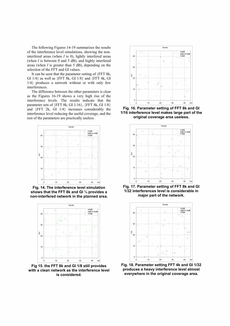
The following Figures 14-19 summarizes the results

of the interference level simulations, showing the non-interfered areas (when I is 0), lightly interfered areas (when I is between 0 and 5 dB), and highly interfered areas (when I is greater than 5 dB), depending on the selection of the FFT and GI values.

It can be seen that the parameter setting of FFT 8k, GI 1/4 as well as FFT 8k, GI 1/8 and FFT 4k, GI 1/4 produces a network without or with only few interferences.

The difference between the other parameters is clear as the Figures 16-19 shows a very high rise of the interference levels. The results indicate that the parameter sets of FFT 8k, GI 1/16, FFT 4k, GI 1/8 and FFT 2k, GI 1/4 increases considerably the interference level reducing the useful coverage, and the rest of the parameters are practically useless.

I levels

0

10

20

30

40

0 10 20 30 40 km

km

I=0dB0dB<I<=5dBI>5dB

Fig. 14. The interference level simulation

shows that the FFT 8k and GI ¼ provides a non-interfered network in the planned area.

I levels

0

10

20

30

40

0 10 20 30 40 km

km


Fig 15. the FFT 8k and GI 1/8 still provides

with a clean network as the interference level is considered.

I levels

0

10

20

30

40

0 10 20 30 40 km

km


Fig. 16. Parameter setting of FFT 8k and GI

1/16 interference level makes large part of the original coverage area useless.

I levels

0

10

20

30

40

0 10 20 30 40 km

kmI=0dB0dB<I<=5dBI>5dB

Fig. 17. Parameter setting of FFT 8k and GI 1/32 interferences level is considerable in

major part of the network.

I levels

0

10

20

30

40

0 10 20 30 40 km

km


Fig. 18. Parameter setting FFT 4k and GI 1/32 produces a heavy interference level almost everywhere in the original coverage area.

I levels

0

10

20

30

40

0 10 20 30 40 km

km


Fig 19. The simulation shows massive

interference levels in the whole planned area with FFT 2k and GI 1/32.

CDF, C/(N+I)

0

0.10.2

0.3

0.40.5

0.6

0.7

0.80.9

1

-50 -40 -30 -20 -10 0 10 20 30 40 50C/(N+I), dB

QPSK, FFT 8k, GI 1/4QPSK, FFT 8k, GI 1/8QPSK, FFT 8k, GI 1/16QPSK, FFT 8k, GI 1/32QPSK, FFT 4k, GI 1/32QPSK, FFT 2k, GI 1/32

Fig. 20. The cumulative C/(N+I) distribution of

different modes. The Figure 20 shows a résumé of the cumulative

C/(N+I) distribution of different modes. By observing the 90% probability in the cell edge (about 95% in the cell area), i.e. 5 % outage probability of the Figure, the mode FFT 8k, GI1/4 provides a minimum of about 9 dB and the set of FFT 8k, GI1/8 and FFT 4k, GI1/4gives about 5 dB in the whole investigated area. It is worth noting that these values are calculated over the whole map of 45km × 45km.

It seems that the QPSK mode would provide a good performance in the investigated area when using the non-interfering FFT 8k, GI 1/4 parameters, whilst 16-QAM gives smaller yet non-interfered coverage area. The advantage of the latter case is the double radio channel capacity compared to the QPSK with greater coverage area.

The parameter set of FFT 8k, GI 1/8 and FFT 4k, GI 1/4 looks to be still useful, providing the possibility to either rise the maximum velocity of the

terminal (FFT 4k), or give more capacity (GI 1/8), but with the cost of useful coverage area due to the increased interference levels.

As for the rest of the parameter settings, the optimal balance can not be achieved due to the very high interference levels.

5. Conclusions

The presented simulation method provides both

geographical and cumulative distribution of the SFN gain and interference levels. The method can thus be used in the detailed optimization of the DVB-H networks. The principle of the simulator is relatively straightforward and the method can be applied by using various different programming languages. In these investigations, a standard Pascal was used for programming the core simulator.

The results show that the radio parameter selection is essential in the detailed planning of the DVB-H network. As the graphical presentation of the results indicate, the effect of the parameter value selection on the interference level and thus on the quality of service can be drastic, which should be taken into account in the detailed planning of DVB-H.

6. References [1] DVB-H Implementation Guidelines. Draft TR 102 377 V1.2.2 (2006-03). EBU. 108 p. [2] Recommendation ITU-R P.1546-3. Method for point-to-area predictions for terrestrial services in the frequency range 30 MHz to 3000 MHz. 2007. 57 p. [3] Masaharu Hata. Empirical Formula for Propagation Loss in Land Mobile Radio Services. IEEE Transactions on Vehicular Technology, Vol. VT-29, No. 3, August 1980. pp 317-325. [4] Editor: Maite Aparicio. Wing TV. Services to Wireless, Integrated, Nomadic, GPRS-UMTS&TV handheld terminals. D6 – Wing TV Common field trials report. Project report, November 2006. 86 p. [5] Editor: Maite Aparicio. Wing TV. Services to Wireless, Integrated, Nomadic, GPRS-UMTS&TV handheld terminals. D8 – Wing TV Country field trial report. Project report, November 2006. 258 p. [6] Editor: Thibault Bouttevin. Wing TV. Services to Wireless, Integrated, Nomadic, GPRS-UMTS&TV handheld terminals. D8 – Wing TV Measurement Guidelines & Criteria. Project report. 45 p. [7] Gerard Faria, Jukka A. Henriksson, Erik Stare, Pekka Talmola. DVB-H: Digital Broadcast Services to Handheld Devices. IEEE 2006. 16 p.

VIII

Publication VIII

“MPE-FEC Performance in Function of the Terminal Speed in Typical DVB-H Radio Channels”

This paper shows case examples of the MPE-FEC performance in laboratory as well as live network in urban and sub-urban area types. Some typical radio parameter values were varied in the laboratory environment in order to identify the indoor performance. In the live network, a set of typical urban and sub-urban indoor cases were studied. Also vehicular tests were carried out in order to identify the relationship between the MPE-FEC performance and vehicular speed.

IEEE International Symposium on Broadband Multimedia Systems and Broadcasting (BMSB)

13-15 May, 2009, Bilbao Spain



mm09-83

1

Abstract—The detailed network planning of DVB-H requires

understanding about the regional differences and their effects on the functionality of the system performance. A deep city center contains various radio components whereas rural area normally consists of a single line-of-sight signal resulting differences in the error behavior in the DVB-H reception. In the city area, the terminal velocity is normally limited to pedestrian and relatively slowly moving vehicular speeds. On the other hand, the Doppler shift might be the limit of DVB-H performance in the motorways across rural areas due to the higher velocities. This paper presents a radio interface quality analysis methodology based on the erroneous frames and bit error rates. A selected set of field and laboratory test cases and respective results of the performance analysis is presented. The results can be used as a basis for balancing the MPE-FEC rate and capacity of DVB-H during the related in-depth radio network optimization.

Index Terms—Field trials and test results, mobile broadcast, mobile TV, DVB-H, radio network planning, performance evaluation, propagation and coverage, radio network planning.

I. INTRODUCTION VB-H (Digital Video Broadcasting, Handheld) is based on the terrestrial version of DVB, i.e. DVB-T, and it has

been designed especially for the moving environment. The performance of the system takes into account the variations of the received power levels and bursty interferences of the radio path. DVB-H is adequate especially for the small handsets as the typical terminal screen size requires only a fraction of the bit stream capacity compared to DVB-T which is meant for the fixed reception with the non-movable antennas located in rooftop.

Unlike in case of DVB-T, the handheld version is typically used in street level which brings challenges for the radio reception due to the varying radio conditions. One of the methods of DVB-H to cope with the Doppler effects and multi-path radio signal propagation is the MPE-FEC (Multi

Manuscript received April 9, 2009. This work was supported in part by

Nokia Siemens Networks which provided the field measurement equipment and test laboratory for the study.

Jyrki T.J. Penttinen is with Nokia Siemens Networks, Av Ronda de Europa 5, 28760 Tres Cantos, Madrid, Spain (e-mail: [email protected]).

Eric Kroon is with Nokia Siemens Networks, Karaportti 2, 02610 Espoo, Finland (e-mail: [email protected]).

Protocol Encapsulator, Forward Error Correction). It is an optional feature of DVB-H and has been defined as an additional functionality compared to the original DVB-T specifications, which uses the basic FEC for the error recovery. Depending on the radio channel type, MPE-FEC enhances the performance of DVB-H by applying an additional error coding to the radio link. As a result, the frame error rate can be lowered and thus the usable coverage area and/or the radio channel capacity can be extended.

This paper presents a field test methodology, results and respective analysis in order to estimate the usability of different MPE-FEC code rates in urban, sub-urban and rural environments, and gives recommendations for the related parameter values taking into account typical terminal velocities per area type.

In order to verify the behavior and level of the link budget enhancement via the MPE-FEC functionality in urban environment, case studies were carried out in laboratory environment as well as in functional urban DVB-H network coverage areas of Helsinki, Finland. The work contains the verification of the behavior of the error correction capabilities of MPE-FEC via field tests and by studying the post-processed data.

Comparative field test measurements were carried out in variable radio channel types, altering the terminal speed around the threshold values for the MPE-FEC. The test cases were repeated in urban, sub-urban and rural areas in order to investigate the effect of the radio channel type on the error correction performance.

II. THE EFFECT OF MPE-FEC ON RADIO NETWORK PLANNING The MPE-FEC that DVB-H uses is based on Reed-Solomon

(RS) code. The DVB-H Implementation Guidelines [1] explains the method, with the possibility to use puncturing. On the other hand, the decoding is left open and the receiver solutions might thus differ from each others. There are various possibilities to decode the signal as indicated in [15].

The IP datagrams of DVB-H are encapsulated into MPE-FEC frame. The time slicing burst size effects on the MPE-FEC in such way that the amount of MPE-FEC rows can be set to 256, 512, 768 or 1024. The datagrams are encapsulated column-wise to the frame, and the encoding is done row-wise with Reed-Solomon variant RS(255,191), indicating that the

MPE-FEC Performance in Function of the Terminal Speed in Typical DVB-H Radio

Channels Jyrki T.J. Penttinen, Member, IEEE, Eric Kroon, Member, IEEE

D

mm09-83

2

total size of the frame is 255 columns, which consists of 191 columns of application data (IP datagrams) and 64 columns of Reed-Solomon data (parity bytes sections and possibly punctured RS fields). The Figure 1 shows the principle of the frame. The final MPE-FEC rate depends on the filling of the data and RS columns, and can be selected from the values of 1/2, 2/3, 3/4, 5/6 or 1/1 (i.e. when no MPE-FEC is used).

IP datagram

1

IP datagram

1IP

datagram 2

IP datagram

2

Padding

Padding

IP datagram

n

Columns 1-191 for the application data

(MPE section)

1st section of parity bytes

2nd section of parity bytes

Last section of parity bytes

1st column of punctured R

S

2nd column of punctured R

S

Last column of punctured R

SColumns 1-64 for the RS data table

(FEC section)

. . .

. . . . . .. . .

Fig. 1. DVB-H frame structure.

The IP datagram consists of IP header (20 bytes) and IP

payload (maximum of 1480 bytes). The IP datagram then consists of MPE header (12 bytes) and CRC-32 check field (4 bytes). On the other hand, the FEC sections (columns) consists of FEC header (12 bytes) and CRC-32 tail (4 bytes). These MPE and FEC packets (with respective MPE or FEC headers) are then fragmented to a transport stream (TS) in such way that TS header (4-5 bytes; 5 if the TS packet contains the first byte of a section) is sent first, then MPE payload (183 bytes) followed by FEC TS header (4 bytes) and FEC payload (184 bytes).

The frame error quality criterion of 5 % has been used in DVB-H radio network quality and limit estimations. The 5 % criteria can be studied when MPE-FEC is not used (frame error rate, FER), or with MPE-FEC involved (MFER, frame error rate after MPE-FEC). The 5 % criterion was originally selected in subjective way in the early phase of DVB-H evaluations, as it provides with practical means of estimating the quality. It is based on the intuitive idea of having maximum of 1 erroneous frame with 1 second of length during 20 seconds of measuring period.

III. METHODOLOGY This study concentrates on the MPE-FEC performance via

the post-processing and analysis of the radio measurement results. The field tests were carried out in mainly urban and rural areas in Helsinki inside of partially overlapping coverage areas of a commercial DVB-H network. Also selected labora-tory measurements were carried out in indoor environment, and vehicular tests in the metropolitan area of Beijing, China.

The field test equipment consisted of the commercial DVB-H terminal and a data collection unit which is based on the available radio interface measurement equipment. All the

relevant performance indicators were collected from the radio interface by storing the results to text files for the further post-processing. The performance identifiers included the received power and packet error levels, carrier to noise level, frame errors before and after the MPE-FEC correction, as well as the bit error rates before and after Viterbi. Also the geographical position was stored to the log files in order to identify the specific location of occurred errors.

In the quality revision of the network, the frame error rate indicates sufficiently well the real performance of the radio network as it is comparable with the end-user’s interpretation of the service quality. More specifically, the DVB-H planning guideline [1] proposes that frame error rate of 5% or less indicates that the reception is sufficiently good as for the user experiences. Furthermore, the [1] shows that the 10% frame error level is already annoying in practical reception.

After the first phase DVB-H evaluation tasks, more in-depth criteria have been searched for. As an example, [16] has concluded that the limit for the acceptable quality based on the subjective interpretation is roughly between 6.9 % and 13.8 % as for the MFER when the channel type is close to vehicular urban (VU). This indicates that the MFER5 might be slightly pessimistic, but it is used in this study for the comparison purposes for the results obtained in other studies.

The level of the MPE-FEC correction can be obtained by investigating what is the level of frame errors (FER, Frame error Rate) compared to the frame errors after the MPE-FEC functionality (MFER, MPE-FEC frame error rate).

In this study, both laboratory and live network tests were carried out. The post-processing of the data was done by exporting the measurement raw data to Excel spreadsheet. The post-processing included the organization of the data to PDF format, received power level representing the x-axis with 1 dB resolution, and MPE-FEC results being the variable as seen in Figure 2.

When the values per RSSI level are normalized to 100 %, the format shows the proportion of the occurred frame errors that could be corrected, arranged in function of the RSSI levels as seen in figure 3. The format gives indication about the general probability distribution of the MPE-FEC functionality in investigated area type in function of RSSI.

For the comparison of the performance with the terminal speed, also a cumulative presentation was calculated for frame error occasions showing the expected success rates of MPE-FEC with different parameter values. This gives indication of the effectiveness of the MPE-FEC per case in different area types, i.e. with what RSSI value the MPE-FEC starts function-ing, and up to what RSSI limit it is still able to correct sufficiently effectively the frame errors. An example of this format can be seen in Figure 4.

In the Figures 2-4, the term “FER1, MFER0” means that there has been frame error which could be recovered by MPE-FEC. “FER1, MFER1” means that the occurred error could not be recovered any more, and “FER0, MFER0” means that there were no frame errors present in the first place.

mm09-83

3

Count of s am ple s per Prx leve l

0

20

40

60

80

100

120

-50

-53

-56

-59

-62

-65

-68

-71

-74

-77

-80

-83

-86

-89

-92

-95

dBm

Cou

nts

FER0, MFER0 #

FER1, MFER0 #

FER1, MFER1 #

Fig. 2. An example of the collected and post-processed data. The RSSI raster is 1 dB, and each RSSI value corresponds to the error-free samples (FER 0), as well as occurred frame errors (FER 1) that could be corrected by MPE-FEC (0) or not (1).

FER and M FER, % per RSSI value

0

10

20

30

40

50

60

70

80

90

100

-50

-54

-58

-62

-66

-70

-74

-78

-82

-86

-90

-94

dBm

%

FER%MFER %10% criter ia5% criteria

Fig. 3. An example of the MPE-FEC analysis.

FER/MFER%, cumulative over the route

0

10

20

30

40

50

60

70

80

90

100

-50

-53

-56

-59

-62

-65

-68

-71

-74

-77

-80

-83

-86

-89

-92

-95

dBm

FER0, MFER0 cum%

FER1, MFER1 cum%FER1, MFER0 cum%

Fig. 4. An example of the cumulative analysis of the measurement data. This format gives idea about the RSSI scale where the MPE-FEC was taken place and where it was effective. In this specific example, the MPE-FEC took place for 80 % of the samples (from 10% to 90% of cumulated values) in about -84.5…-89.5 dBm scale creating a 5 dB window for the functional MPE-FEC.

IV. THE CASE SETUP The investigation of the frame error correction capability of

DVB-H was divided into three parts: Laboratory tests, indoor tests in live network and vehicular tests in live network. The setup consisted of commercial DVB-H terminals with additional software developed by Nokia for the logging of the relevant measurement values in the radio interface as described in [13] with the respective analysis method.

A. Laboratory tests In the laboratory tests, the 16-QAM was selected for the

modulation method. In each test case, code rate of 1/2 was utilized, as well as FFT 8k and GI 1/4. The MPE-FEC rate was varied between 15% (5/6), 25% (3/4) and 35% (2/3).

The test setup consisted of one radiating DVB-H indoor antenna (omni-pole with about +2 dBi gain in horizontal plane). There was a complete DVB-H core and radio network in use. The radio transmitter was adjusted to 250 mW input power level, which was fed to the antenna cable of about 15 meters of length and about 7 dB loss per 100 m. The core network of the setup captured live audio/video content and delivered it in DVB-H format to the radio interface. The Table 1 shows the channel configuration for each test case.

The measurements took place in indoor environment as

presented in the Figure 5. There was a single corridor where the cell limits as well as the MPE-FEC performance areas were identified.

50 m

TX

RX

Fig. 5. The measurement area for the laboratory cases.

The terminal speed was kept constantly about 1-2 m/s, i.e. keeping the terminal in constant slow motion with walking speed. The aim was to collect sufficiently data especially around the breaking point of the RSSI scale, i.e. where MPE-FEC takes place.

B. Indoor tests in live network The indoor tests were carried out in the downtown area of

Helsinki by observing the performance of the live DVB-H network. In this specific case, the radio network covered the city area and sub-urban of Helsinki, with partially overlapping

TABLE 1. THE DVB-H LABORATORY CHANNEL CONFIGURATION.

Case CR FEC PID FEC rows A 50% 15% 1024 512 B 50% 25% 1280 512 C 50% 35% 1536 768

mm09-83

4

areas in SFN mode. The aim was to identify cell edge areas inside the typical public buildings like shopping centers.

For the comparison purposes, also the respective outdoor measurement was done. This merely shows the received power level compared to the indoor cases, as there was practically no frame errors observed in the measurement points of the outdoor environment.

During the measurements, the relevant radio interface parameters were the following: 16-QAM modulation, FFT 8k, GI 1/8, code rate 1/2, MPE-FEC rate 5/6 (15%).

C. Vehicular tests As a third part of the study, there were outdoor measure-

ments carried out by using a vehicle mounted calibrated field tester. The aim was to collect the performance indicators in variable vehicle speeds and different environments from the city center, sub-urban and rural areas.

During the drive test an outside mounted antenna was used for the reception of the radio signal. The testing was conducted in three stages. The first stage was conducted within the city of Helsinki and Espoo (urban and sub-urban environment) where the same route was drives with different speeds to find the speed where the FER are starting to happen. The speeds driven were 20 km/h, 40 km/h and 60 km/h. The environment chosen was excellent (received power level RSSI limit minimum of -75 dBm and C/(N+I) > 15 dB). This environment was chosen to eliminate all possibilities of degradation of the signal other then the speed. The second stage was conducted on the highway in urban areas in the greater Helsinki area and the speed tested were 80 km/h, 100 km/h and 120 km/h, again with excellent conditions. Both cases were conducted with the UdCast Navigator. In the third and final stage a drive test was conducted in the metropolitan area of Beijing in different speeds in an urban environment. Measurement equipment used was the Rohde&Schwarz TSM-DVB-H scanner.

Finland network settings were: 16-QAM, CR 1/2, MPE-FEC 1/2, GI 1/8. China network settings were: QPSK, CR 1/2, MPE-FEC= 1/2, GI = 1/8.

V. RESULTS AND ANALYSIS

A. Laboratory tests The following Table 2 summarizes the laboratory test cases

and respective results for the MPE-FEC breaking points (i.e. showing the RSSI values with the 5 % criteria) in received power levels (dBm) when using 16-QAM, code rate of 1/2, FFT of 8k and GI of 1/8. In this case, there were 2 terminals used in the data collection, Nokia models N-77 (terminal 1) and N-96 (terminal 2). As the results show, the terminals were not commonly calibrated as for the RSSI display. Neverthe-less, the relative frame error information with and without MPE-FEC per terminal can be obtained even without the information about the exact RSSI breaking point.

As the Table 2 shows, the difference between FER5 and

MFER5 grows as the MPE-FEC rate grows, i.e. there is a logical behavior noted for the frame error capability in function of the MPE-FEC rate in all of the cases. In the least protected mode (MPE-FEC 15%), the difference, i.e. the MPE-FEC gain, is close to zero. This can be explained by the building layout, which did not allow too much multipath components in the receiving end. In the most protected mode that was applied in these measurements (MPE-FEC 35%), the MPE-FEC gain is in order of 2 dB. The MPE-FEC rate of 25% seems to result only about 0.5 dB gain.

This case study shows that the MPE-FEC gain is not relevant in indoor environment with low amount of reflected multipath components in radio interface and with slowly moving terminal, if the MPE-FEC rate is defined to 15% or 25%. The effect starts to be notable when using MPE-FEC rate of 35%, giving about 2 dB gains compared to the situation without MPE-FEC in the investigated channel types (which are close to typical urban 3, or TU3 type of models). On the other hand, this 35% MPE-FEC rate reduces accordingly the capacity that can be offered in the radio interface.

B. Indoor tests in live network The following Table 3 summarizes the post-processed in-

door measurement results for the city area of Helsinki, i.e. the breaking points of FER 5% and MFER 5% in function of the received power level (dBm). The “counts” column summa-rizes the amount of collected measurements (frames) per case. The cases are the following.

“A” represents a ground floor of a shopping center with relatively large open areas. It can be estimated that some multi-path propagated components arrived to the measurement routes.

“B” represents another relatively large shopping center in the very center of the city. There are probably plenty of multipath component present in this environment.

“C” represents the ground floor of a relatively large 2-floor bookstore with open center area.

“D” is the upper floor of the case “C”. “E” is the ground floor of a very large shopping center in

the city center. “F” is the upper floor of the case “E”. “G”, “H” and “I” represents the ground, second and third

floor of university campus building in sub-urban area.

TABLE 2. THE DVB-H LABORATORY MEASUREMENT RESULTS. *THE GAIN COULD

NOT BE SEEN EXPLICITLY DUE TO THE INSTABILITY IN MFER5 POINT. Case / FEC Terminal FER5 MFER5 Diff

A / 15% 1 -78.0 -78.05 0.05 B / 25% 1 -77.1 -77.5 0.4 C / 35% 1 -68.8 -70.7 1.9 A / 15% 2 -83.2 -83.4 0.2 B / 25 % 2 -81.0 -81.0/-83.2 0.0/2.1 * C / 35% 2 -82.5 -84.5 2.0

mm09-83

5

Note 1. The environment contained impulse noise sources

probably due to the power systems of the mechanical escala-tors. The Figure 6 shows the behavior of the effect.

Note 2. There were relatively low amount of data collected in this case which affects on the statistical accuracy. There was also probably an impulse noise peak in FER figure which adds uncertainty to the interpretation of the corresponding MPE-FEC gain. Nevertheless, the MPE-FEC could correct the occurred interference peak.

Note 3. The received power level was too high in this area in order to interpret the MPE-FEC effect.

FER and MFER (re sults in scale 0-20 % pe r Prx value )

0

5

10

15

20

-50

-52

-54

-56

-58

-60

-62

-64

-66

-68

-70

-72

-74

-76

-78

-80

-82

-84

-86

-88

-90

-92

-94

-96

dBm

%

FER%MFER %10% criter ia5% criter ia

Fig. 6. An example of the impulse type of noise that affected on the measurements in case B.

The results obtained from the laboratory environment are a

bit more pessimistic compared to the dense urban indoor results. With 15% of MPE-FEC rate and common parameter set, the laboratory cases showed a maximum of 0.2 dB gains whereas city center’s indoor environment provided up to 1 dB gains. This is due to the varying multipath components in radio interface, laboratory being more limited in this sense. In sub-urban environment, though, the indoor gain was around in the same low level as was obtained in laboratory.

C. Vehicular tests From the first drive test results no errors were found until

60 km/h. The errors started to appear with higher speeds. The following figure represents the CDF of the BER with different speeds. The 50% point is at 80 km/h.

BER cummulative over the route

0%

20%

40%

60%

80%

100%

0 7 17 22 31 36 41 47 52 58 63 71 77 82 87 92 97 102

107

speed (km/h)

% B

ER s

ampl

es

CDF

Fig. 7. BER analysis as a function of the terminal speed measured in Finland .

The following graph shows the average PER (non

correctable RS packets over the total received packets [17]) and the BER (Bit Error Rate before RS) in relation to the speed from the China measurements. From the graph can be seen that around 65 km/h the PER (> 5000 packets/sec) and BER (> 2⋅10-3) are getting high. This is due to the challenging environment, which consists of densely packed flat buildings which create many multipath fading signals.

BER and PER in relation to speed

0

5000

10000

15000

20000

25000

0 5 10 15 20 25 30 35 40 45 50 55 60 65 70

Speed (km/h)

PER

(avg

pac

ket l

oss/

sec

)

0

0,001

0,002

0,003

0,004

0,005

0,006

0,007

0,008

BER

(%)

PERBER

Fig. 8. PER and BER as a function of the speed measured in China

It can be seen from the Figure 8 that the 50% BER point is

at 63 km/h.

BER Cummulative over the route

0%

20%

40%

60%

80%

100%

0 5 10 15 20 25 30 35 40 45 50 55 60 65 70 75 80

Speed

cdf

CDF BER

Fig. 9. BER CDF measured in China

VI. MPE-FEC OPTIMIZATION The analysis shows that the MPE-FEC is normally useful

only when the received power level is low enough. The Figure 4 shows the basic principle of the functional scale of MPE-FEC, indicating that the RSSI window where MPE-FEC “wakes up” and is able to correct the erroneous frames is relatively small and near the performance limits of the cell. This means, that in decent and good radio field, MPE-FEC does not give added value even if there are multi-propagated

TABLE 3. THE DVB-H INDOOR MEASUREMENT RESULTS.

Case Counts Max speed FER5 MFER5 Diff

A 1022 1-2 m/s -84.5 -85.5 1.0 B 1 532 1-2 m/s N/A N/A N/A C 2 181 1-2 m/s -85.2 -87.4 2.2 D 3 238 1-2 m/s N/A N/A N/A E 556 1-2 m/s -79.0 -80.1 1.1 F 518 1-2 m/s -87.4 -88.0 0.6 G 506 1-2 m/s -85.4 -85.4 0.0 H 506 1-2 m/s -87.1 -87.3 0.2 I 515 1-2 m/s -88.3 -88.8 0.5

mm09-83

6

radio components present. This applies for the indoor and outdoor pedestrian and vehicular environments. With the used parameter set, the Doppler shift was not the limiting factor.

The drive test results show that the speed for the BER breakpoint is around 80 km/h in perfect conditions and -65 dBm in challenging environments.

The lowest MPE-FEC rates result only minor enhancement in indoor environment based on the laboratory measurements and the FER/MFER analysis. MPE-FEC gain was about 0.5 dB or less for 25% MPE-FEC rate, and near zero for 15% MPE-FEC rate. For 35% MPE-FEC rate, values of about 2 dB were observed for the MPE-FEC gain. The Table 4 summa-rizes the averaged MPE-FEC gain results and the respective standard deviation values for laboratory, city indoor, sub-urban indoor and sub-urban motorway cases when analyzed via FER and MFER differences and MPE-FEC 15% was used.

As the MPE-FEC reserves a proportion of capacity from the

total radio channel bandwidth, the balancing of the capacity and the MPE-FEC gain should be planned according to the operational environment. Based on this analysis, it would be recommendable to limit the MPE-FEC rate to lower values of the scale as it reserves thus only small proportion of the capacity but still corrects at some extend the occurred frame errors. This would be justified in indoor environment even with the multi-propagated radio paths as the field tends to drop fast in the cell edge according to the laboratory and indoor field measurements carried out in this study. On the other hand, in the typical urban and dense urban environment, the DVB-H radio coverage is normally good enough in order to provide decent indoor coverage. This means that the field in outdoor is so high that MPE-FEC is not normally needed, but recommendable due to multipath fading.

Also sub-urban area within the DVB-H coverage seems to benefit only little from MPE-FEC. In the buildings, the gain seems to be even less than in urban areas due to the lower amount of multipath components. Nevertheless, approaching the service area edge, the field strength is sufficiently low in order to activate the MPE-FEC, which brings about 1 dB MPE-FEC gain in normal motorway environment with the lowest MPE-FEC rate.

VII. CONCLUSIONS In the in-depth DVB-H network planning, the fine-tuning

of the relevant radio parameters is essential for different geographical clutter types. This study presents the MPE-FEC test methodology which is based on the collection of the relevant radio performance indicators via the field test

equipment. Furthermore, an analysis of the MPE-FEC behavior was done in order to seek the optimal functional radio parameter values in the investigated area types.

This paper describes the methodology that can be applied for DVB-H radio reception error level measurements and analysis in order to identify the optimal MPE-FEC rate parameter values in different network environments. The outcome of the study is the optimal MPE-FEC parameter value set for the typical DVB-H environments in function of the terminal velocity. The paper also shows that MPE-FEC can be altered in different DVB-H areas, although the tuning of the parameter should be done based on the field measurements of individual cases as the carrier per noise level varies in each network setup.

REFERENCES [1] DVB-H Implementation Guidelines. Draft TR 102 377 V1.2.2 (2006-

03). European Broadcasting Union. 108 p. [2] Editor: Thibault Bouttevin. Wing TV. Services to Wireless, Integrated,

Nomadic, GPRS-UMTS&TV handheld terminals. D8 – Wing TV Measurement Guidelines & Criteria. Project report. 45 p.

[3] Editor: Maite Aparicio. Wing TV. Services to Wireless, Integrated, Nomadic, GPRS-UMTS&TV handheld terminals. D6: Common field trials report. November 2006. 86 p.

[4] Editor: Maite Aparicio. Wing TV. Services to Wireless, Integrated, Nomadic, GPRS-UMTS&TV handheld terminals. Wing TV Country field report. November 2006. 258 p.


[6] Joan Mazenc. Multi protocol Encapsulation – Forward Error Correction (MPE-FEC). ETUD/Insa. Toulouse, France, January 9, 2007. 7 p.

[7] G. Gardikis, H. Kokkinis, G. Kormentzas. Evaluation of the DVB-H data link layer. European Wireless 2007. 1-4 April 2007, Paris, France. 6 p.

[8] Heidi Joki, Jarkko Paavola. A Novel Algorithm for Decapsulation and Decoding of DVB-H Link Layer Forward Error Correction. Department of Information Technology, University of Turku. 6 p.

[9] Masaharu Hata. Empirical Formula for Propagation Loss in Land Mobile Radio Services. IEEE Transactions on Vehicular Technology, Vol. VT-29, No. 3, August 1980. 9 p.

[10] Recommendation ITU-R P.1546-3. Method for point-to-area predictions for terrestrial services in the frequency range 30 MHz to 3000 MHz. 2007. 57 p.

[11] Tero Jokela, Eero Lehtonen. Reed-Solomon Decoding Algorithms and Their Complexities at the DVB-H Link-Layer. Turku Centre for Computer Science, Department of Information Technology, University of Turku. 5 p.

[12] ETSI EN 301 192, V1.4.1 (2004-11). Digital Video Broadcasting (DVB); DVB specification for data broadcasting. European Telecommunications Standards Institute 2004. 78 p.

[13] Penttinen, J. Field Measurement and Analysis Method for DVB-H Terminals. The Third International Conference on Digital Telecommunication. ICDT 2008, 29.6.-5.7. 2008 – Bucharest, Romania. 6 p.

[14] D. Plets, W. Joseph, L. Verloock, E. Tanghe, L. Martens, E. Deventer, H. Gauderis. Influence of Reception Condition, MPE-FEC Rate and Modulation Scheme on Performance of DVB-H. IEEE Transactions on Broadcasting, Vol. 54, No. 3, September 2008. Pp. 590-598.

[15] J. Paavola, H. Himmanen, T. Jokela, J. Poikonen, V. Ipatov. The Performance Analysis of MPE-FEC Decoding Methods at the DVB-H Link Layer for Efficient IP Packet Retrieval. IEEE Transactions on Broadcasting, Vol. 53, No. 1, March 2007. Pp. 263-275.

[16] H. Himmanen. Studies on Channel Models and Channel Characteristics for Mobile Broadcasting. Department of Information Technology, University of Turku, Turcu Centre for Computer Science, Finland. 9 p.

[17] IP datacast over DVB-H : Implementation guidelines for mobility, DVB document A117, DVB organization, July 2007, p 18-19

TABLE 4. THE SUMMARY OF THE MPE-FEC GAINS IN DIFFERENT ENVIRONMENTS.

Environment Average Stdev Laboratory 0.1 0.1

Urban indoor 1.2 0.7 Sub-urban indoor 0.2 0.3

Sub-urban motorway 1.0 N/A

IX

Publication IX

“Field measurement and data analysis method for DVB-H mobile devices”

The paper is an extended version of the Publication II. The paper was invited to the journal as a result of the further evaluation of the conference paper. This extended version shows more thoroughly the measurement methodology, and shows in deeper level the analysis of the field test results by dividing the investigated area into specific radio propagation channel types.

International Journal On Advances in Systems and Measurements, issn 1942-261x, vol. 2, no. 1, year 2009, pages 18 - 32

http://www.iariajournals.org/systems_and_measurements/



Field Measurement and Data Analysis Method for DVB-H Mobile Devices


[email protected]

Abstract

The field measurement equipment that provides

reliable results is essential in the quality verification of DVB-H networks. In addition, sufficiently in-depth analysis of the post-processed data is important. This paper is based on [12] and presents a method to collect and analyze the key performance indicators of the DVB-H radio interface, using a mobile device as a measurement and data collection unit. 1. Introduction

The verification of the DVB-H quality of service level can be done by carrying out field measurements within the coverage area. Correct way to obtain the most relevant measurement data, as well as the right interpretation of it, are fundamental for the detailed network planning and optimization.

During the normal operation of the DVB-H network, there are only few possibilities to carry out long-lasting and in-depth measurements. A simple and fast field measurement method based on mobile DVB-H receiver provides thus added value for the operator. The mobile equipment is easy to carry both in outdoor and indoor environment, and it stores sufficiently detailed performance data for the post-processing.

The measurements are required for the network performance revisions and for the indication of potential problems. As an example, the transmitter site antenna element might move due to the loose mounting, which results outages in the designed coverage area. The antenna feeder might still remain connected correctly, keeping the reflected power in acceptable level. As there are no alarms triggered in this type of instance, and as the basic DVB-H is a broadcast system without uplink and its related monitoring / alarming system, the most efficient way to verify this kind of fails is to carry out field tests.

This paper presents a method to post-process the basic field test data collected with DVB-H mobile

terminal. The method can be considered as an addition to the usual network performance testing carried out by the operator and is suitable for the fast revisions of the radio quality levels and possible network faults.

The results presented in this paper are meant as examples and for clarifying the analysis methodology. The data was collected with a commercial DVB-H hand-held terminal capable of measuring and storing the radio link related data. In this specific case, a Nokia N-92 terminal was used with a field test program. The program has been developed by Nokia for displaying and storing the most relevant DVB-H radio performance indicators.

2. Coding of DVB-H

In order to carry the DVB-H IP datagrams of the

MPEG-2 Transport Stream (TS), a Multi Protocol Encapsulator (MPE) is defined for DVB. Each IP datagram is encapsulated into single MPE section. Elementary Stream (ES) takes care of the transporting of these MPE sections. Elementary Stream is thus a stream of packets belonging to the MPEG-2 Transport Stream and with a respective program identifier (PID). The MPE section consists of 12 byte header, 4 byte CRC-32 (Cyclic Redundancy Check), as well as a tail and payload length. [4]

The main idea of MPE-FEC is to protect the IP datagrams of the time sliced burst with an additional link layer Reed-Solomon (RS) parity data. The RS data is encapsulated into the same MPE-FEC sections of the burst with the actual data. The RS part of the burst belongs into the same elementary stream (MPE-FEC section), but they have different table identifications. The benefit of this solution is that the receiver can distinguish between these sections, and if the terminal does not have the capability to use the DVB-H specific MPE-FEC, it can anyway decode the bursts although with lower quality when it experiences difficult radio conditions. [13, 14, 15, 16]

The part of the MPE-FEC frame that includes the IP datagrams is called application data table (ADT). ADT

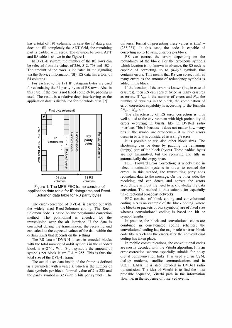
has a total of 191 columns. In case the IP datagrams does not fill completely the ADT field, the remaining part is padded with zeros. The division between ADT and RS table is shown in the Figure 1.

In DVB-H system, the number of the RS rows can be selected from the values of 256, 512, 768 and 1024. The amount of the rows is indicated in the signaling via the Service Information (SI). RS data has a total of 64 columns.

For each row, the 191 IP datagram bytes are used for calculating the 64 parity bytes of RS rows. Also in this case, if the row is not filled completely, padding is used. The result is a relative deep interleaving as the application data is distributed for the whole bust. [7]

Punctured

columns

Padded

space

Padded

spacePadded

space

RS paritybytes

IP datagrams

.

.

.

.

.

....

First byte (element)

256, 512, 768 or1024 rows

191 datacolumns

64 RScolumns

Figure 1. The MPE-FEC frame consists of application data table for IP datagrams and Reed-

Solomon data table for RS parity bytes.

The error correction of DVB-H is carried out with the widely used Reed-Solomon coding. The Reed-Solomon code is based on the polynomial correction method. The polynomial is encoded for the transmission over the air interface. If the data is corrupted during the transmission, the receiving end can calculate the expected values of the data within the certain limits that depends on the settings.

The RS data of DVB-H is sent in encoded blocks with the total number of m-bit symbols in the encoded block is n=2m-1. With 8-bit symbols the amount of symbols per block is n= 28-1 = 255. This is thus the total size of the DVB-H frame.

The actual user data inside of the frame is defined as a parameter with a value k, which is the number of data symbols per block. Normal value of k is 223 and the parity symbol is 32 (with 8 bits per symbol). The

universal format of presenting these values is (n,k) = (255,223). In this case, the code is capable of correcting up to 16 symbol errors per block.

RS can correct the errors depending on the redundancy of the block. For the erroneous symbols which location is not known in advance, the RS code is capable of correcting up to (n-k)/2 symbols that contains errors. This means that RS can correct half as many errors as the amount of redundancy symbols is added in the block.

If the location of the errors is known (i.e., in case of erasures), then RS can correct twice as many erasures as errors. If Nerr is the number of errors and Ners the number of erasures in the block, the combination of error correction capability is according to the formula 2Nerr + Ners < n.

The characteristic of RS error correction is thus well suited to the environment with high probability of errors occurring in bursts, like in DVB-H radio interface. This is because it does not matter how many bits in the symbol are erroneous – if multiple errors occur in byte, it is considered as a single error.

It is possible to use also other block sizes. The shortening can be done by padding the remaining (empty) part of the block (bytes). These padded bytes are not transmitted, but the receiving end fills in automatically the empty space.

FEC (Forward Error Correction) is widely used in telecommunication systems in order to control the errors. In this method, the transmitting party adds redundant data to the message. On the other side, the receiving end can detect and correct the errors accordingly without the need to acknowledge the data correction. The method is thus suitable for especially uni-directional broadcast networks.

FEC consists of block coding and convolutional coding. RS is an example of the block coding, where the blocks or packets of bits (symbols) are of fixed size whereas convolutional coding is based on bit or symbol lengths.

In practice, the block and convolutional codes are combined in concatenated coding schemes; the convolutional coding has the major role whereas block code like RS cleans the errors after the convolutional coding has taken place.

In mobile communications, the convolutional codes are mostly decoded with the Viterbi algorithm. It is an error-correction scheme especially suitable for noisy digital communication links. It is used e.g. in GSM, dial-up modems, satellite communications and in 802.11 LANs. It is also included in DVB-H radio transmission. The idea of Viterbi is to find the most probable sequence, Viterbi path in the information flow, i.e. in the sequence of observed events.

The MPE-FEC has been designed taking into account the backwards compatibility. DVB-T de-modulation procedure contains error correction so both DVB-T and DVB-H utilizes it for the basic coding with Viterbi and Reed-Solomon decoding, whereas DVB-H can use also a combination of Viterbi, Reed-Solomon and additional MPE-FEC to improve the C/N and Doppler performance. [13] The detection of the presence of MPE-FEC is done based on the single demodulated TS packet, as its header contains the error flag. MPE-FEC adds the performance in moving environment as it uses so called virtual interleaving over several basic FEC sections.

In this study, the bit rates before and after the Viterbi as well as the frame error rates of DVB-H MPE-FEC and DVB-T specific FEC were observed by collecting and analyzing data in radio interface. The measurement principles of WingTV guidelines [3] were taken into consideration in the selection (limiting) of the parameter values.

The guideline defines the MFER (MPE Frame Error Ratio) as a ratio of the number of residual erroneous frames that can not be recovered to the total number of the received frames:

framesreceivedframeserroneousresidualMFER

___100(%) =

There are possibilities to obtain the MFER value by

storing the frames during certain time (e.g. 20 seconds), or as proposed by DVB, at least 100 frames should be collected in order to calculate the MFER with sufficient statistical reliability.

The measurement principles of WingTV was used as a basis in the study by collecting 25 minutes of field data during a drive test with varying speeds, and the data was later post-processed in order to obtain the more specific relation between the FER, MFER and received power level categories. Although WingTV does not recommend the use of QEF as a criterion, also the bit errors were analyzed by utilizing the same principles for the comparison purposes. 3. Test setup

A test setup with a functional DVB-H transmitter site was utilized in order to investigate the presented field test methodology with respective post-processing and analysis. The site antenna safety distance zones were estimated by applying [9]. The investigated area represents relatively open sub-urban environment as shown in the Figure 2. There are mainly relatively small trees, residential areas and highways in the

investigated area with nearly-LOS in major part of the investigated area.

Figure 2. The environment in main lobe of the

transmitter antenna.

The methodology was verified by carrying out various field tests mostly in vehicle. There was also static and dynamic pedestrian type of measurements included in the test cases in order to verify the usability of the equipment and methodology for the analysis.

The DVB-H test network consisted of a single 200 watt DVB-H transmitter and a basic DVB-H core network. The source data was delivered to the radio interface by capturing real-time television program. The program was converted to DVB-H IP data stream with standard DVB-H encoders. There was a set of 3 DVB-H channels defined in the same radio frequency, with audio / video bit rates of 128, 256 and 384 kb/s. The number of FEC rows was selected as 256 for MPE-FEC rate of ½, and 512 for MPE-FEC rate of 2/3. The audio part of the channel was coded with AAC using a total of 64 kb/s for stereophonic sound. The bandwidth was 6 MHz in 701 MHz frequency.

The antenna system consisted of directional antenna panel array with 2 elements as shown in Figure 3. Each element produces 65 degrees of horizontal beam width and provides a gain of +13.1 dBi.

Figure 3. The antenna system setup.

The vertical beam width of the single antenna

element was 27 degrees, which was narrowed by locating two antennas on top of each others via a

power splitter. Taking into account the loss of cabling, jumpers, connectors, power splitter and transmitter filter, the radiating power was estimated to be +62.0 dBm (EIRP) in the main lobe.

The transmitter antenna system was installed on a rooftop with 30 meters of height from the ground. The environment consisted of sub-urban and residential types with LOS (line-of-sight) or nearly LOS in major part of the test route, excluding the back lobe direction of the site which was non-LOS due to the shadowing of the site building. Each test route consisted of two rounds in the main lobe of the antenna with a minimum received power level of about -90 dBm. The maximum distance between the antenna system and terminals was about 6.4 km during the drive tests.

If the relevant data can be measured from the radio interface and stored in text format, the method presented in this paper is independent of the terminal type. It is important to notice, though, that the characteristics of the terminal affects on the analysis, i.e. the terminal noise factor and the antenna gain (which is normally negative in case of small DVB-H terminals) should be taken into account accordingly. On the other hand, unlike with the advanced field measurement equipment, the method gives a good idea about the quality that the DVB-H users observe in real life as the terminal type with its limitations is the same as used in commercial networks.

Figure 4. The terminal measurement setup.

There were a total of 3 terminals used in each test

case for capturing the radio signal simultaneously. Multiple receptions provide respectively more data to be collected at the same time, which increases the statistical reliability of the measurements. It also makes possible the comparison of the differences between the terminal performances.

The terminals were kept in the same position inside the vehicle without external antenna, and the results of each test case were saved in separate text files. The terminal setup is shown in the Figure 4. The external antenna was not used because the aim was to revise the quality that the end-user experiences in normal conditions inside the moving vehicle. On the other hand, the test cases were not designed for certain coverage area, but the aim was to classify the performance indicators in function of the received power levels. It does not matter thus if the received power level is interpreted via external or internal antenna. 4. Terminal measurement principles

The DVB-H parameter set was adjusted according to each test case. The cases included the variation of the code rate (CR) with the values of ½ and 2/3, MPE-FEC rate with the values of ½ and 2/3 and interleaving size FFT with the values of 2k, 4k, 8k, in accordance with the Wing TV principles described in [3], [4], [5] and [6]. The guard interval (GI) was fixed to ¼ in each case. The parameter set was tuned for each case, and the audio / video stream was received with all the terminals by driving the test route two consecutive times per each parameter setting.

The needed input for the field test is the “on” and “off” time of the time sliced burst, PID (Packet Identifier) of the investigated burst, the number of FEC rows and the radio parameter values (frequency, modulation, code rate and bandwidth). The terminal stores the measurement results to a log file after the end of each burst until the field test execution is terminated.

According to the DVB-H implementation guide-lines [1], the target quality of service is the following: • For the bit error rate after Viterbi (BA), the

reception should comply at least DVB-H specific QEF (quasi error free) point 2⋅10-4.

• The frame error rate should be less than 5%. In case of FER, i.e. DVB-T, this criterion is called FER5, and for the DVB-H specific MPE-FEC, its name is MFER5.

The field test software of N-92 is capable of collecting the RSSI (received power levels in dBm), FER (Frame Error Rate) and MFER (MPE Frame Error Rate, i.e. FER after MPE-FEC correction) values. In addition, there is possibility to collect information about the packet errors.

The Figure 5 shows a high-level block diagram of the DVB-H receiver. [1] The reception of the Transport Stream (TS) is compatible with DVB-T

system, and the demodulation is thus done with the same principles also in DVB-H. The additional DVB-H specific functionality consists of Time Sliced burst handling, MPE-FEC module and the DVB-H de-encapsulation.

DVB-H specificfunctionality

IP output

DVB-TDemodulator

DVB-HTime Slicing

DVB-HMPE-FEC

DVB-HDe-encapsulation

FER reference

MFER reference

IP reference

TS reference

RF reference

Figure 5. A principle of the reference DVB-H

terminal.

As can be seen from the Figure 5, the FER information, i.e. frame errors before MPE-FEC specific analysis, is obtained after the Time Slicing process, and the MFER is obtained after the MPE-FEC module. If the data after MPE-FEC is free of errors, the respective data frame is de-encapsulated correctly and the IP output stream can be observed without disturbances.

The measurement point for the received power level is found after the antenna element and the optional GSM interference filter. In addition, there might be optional external antenna connector implemented in the terminal before the RF reference point. The presence of the filter and antenna connector has thus frequency-dependent loss effect on the measured received power level in the RF point.

The Figure 6 shows an example of the measurement data file. The example shows 4 consecutive test results. Each measurement field contains information about the occurred frame error (FER), frame error after MPE-FEC correction (MFER), bit error rate before Viterbi (BB) and after Viterbi (BA), packet errors (PA) and received power level (RSSI) in dBm. In this case, there was a frame error in the reception of the first measurement sample because the value of FER was “1”. The FER value is either “0” for non-erroneous or “1” for erroneous frame. The MPE-FEC procedure could still recover the error in this case, because the MFER parameter is showing a value of “0”. The second sample shows that there were no frame errors before or after the MPE-FEC. The third sample shows again frame error that could be corrected with MPE-FEC. The fourth sample shows an error that could not

be corrected any more with MPE-FEC. In the latter case, the bit error information could not be calculated either. It seems that in this specific case, the RSSI value of about -87 dBm to -89 dBm has been the limit for the correct reception of the frames with MPE-FEC.

Figure 6. Example of the measured objects with four consecutive results for FER, MFER, BB, BA,

PE and RSSI.

The plain measurement data has to be post-processed in order to analyze the breaking points for the edge of the performance. Microsoft Excel functionality was utilized in order to arrange the data in function of the received power levels.

According to the first sample of the Figure 6, the bit error level before Viterbi (BB) was close to the QEF point, i.e. 2.5⋅10-2. The bit error level after the Viterbi (BA) was 1.2⋅10-3 which is already better than the QEF point for the acceptable reception. The bit error rate had been thus low enough for the correct reception of the signal. In this example, the amount of packet errors (PE) was between 7 and 75, and the averaged received power level was measured and averaged to -87…-89 dBm. It is worth noting that the RSSI resolution is 1 dB for single measurement event in the used version of the field test software.

The Figure 7 shows the measured RSSI values during the complete test route. There were two rounds done during each test. The back lobe area of the test route can be seen in the middle of the Figure, with fast momentarily drop of received power level. The received power level was about -50 dBm close to the site, and about -90 dBm in the cell edge. The duration of the single test route was approximately 25 minutes, and the total length of the route was 22.4 km.

The maximum speed during the test route was about 90 km/h, and the average speed was measured to 50 km/h (excluding the full stop periods). The speed is sufficient for identifying the effect of the MPE-FEC.

Received power level

-90

-85

-80

-75

-70

-65

-60

-55

-50

-45

-40200 400 600 800 1000 1200 1400 1600 1800

Sample #

RSS

I (dB

)

Fig. 7. The RSSI values measured during the test

route. The following Figures 8 and 9 present the estimated

coverage area for QPSK and 16-QAM cases with the code rate of ½ and MPE-FEC rate of ¾. The Okumura-Hata based propagation model [10] was used with a digital map that contains the elevation data and cluster type information. The minimum received outdoor power level limit for QPSK was estimated as -84 dBm and for 16-QAM as -78 dBm.

The 80 % area location probability criterion was used in these coverage plots. The grid size is 1.6 km. (Background map source: Google Map).

Figure 8. The predicted coverage area for 16-

QAM. The raster shown in the map is 1.6 km. The main lobe and the test route is to north-west

direction form the site.

Figure 9. The predicted coverage area for QPSK,

with the raster size of 1.6 km.

Based on the coverage plots, the test route was selected accordingly. The coverage plots correlated roughly with the drive tests, although the in-depth location-dependent signal level measurements were not carried out during this specific study.

5. Method for the analysis

The collected data was processed accordingly in order to obtain the breaking points, i.e. the QEF of 2 ⋅ 10-4 and FER / MFER of 5% in function of the RSSI values for each test case. The processing was carried out by arranging the occurred events per RSSI value. For the BB and BA, the values were averaged per RSSI resolution of 1 dB. For the FER and MFER, the values represent the percentage of the erroneous frames compared to the total frame count per each individual RSSI value (with the resolution of 1 dB).

The following Figure 10 shows an example of the processed data for the bit error rate before and after the Viterbi for 16-QAM, CR 2/3, MPE-FEC 2/3 and FFT 2k. The results represent the situation over the whole test route in location-independent way, i.e. the results show the collected and averaged BB and BA values that have occurred related to each RSSI value in varying radio conditions.

As can be noted in this specific example, the bit error rate before Viterbi does not comply with the QEF criteria of 2⋅10-4 even in relatively good radio conditions, whereas the Viterbi clearly enhances the performance. The resulting breaking point for the QEF

with Viterbi can be found around -78 dBm of RSSI in this specific case.

BB and BA, average for each Prx value

1.00E-08

1.00E-07

1.00E-06

1.00E-05

1.00E-04

1.00E-03

1.00E-02

1.00E-01

1.00E+00

-50

-54

-58

-62

-66

-70

-74

-78

-82

-86

-90

-94

dBm

BER

QEF

BB ave

BA ave

Figure 10. Post-processed data for the bit error

rate before and after the Viterbi presented in logarithmic scale.

BB and BA averaged for each Prx value

0.0E+00

1.0E-04

2.0E-04

3.0E-04

4.0E-04

5.0E-04

-50

-52

-54

-56

-58

-60

-62

-64

-66

-68

-70

-72

-74

-76

-78

-80

-82

-84

-86

-88

dBm

QEFBA aveBB ave

Figure 11. Processed data for the bit error rate

before and after the Viterbi with an amplified view around the QEF point in linear scale.

For the frame error rate, the similar analysis yields

an example that can be observed in Figure 12. The Figure shows the occurred frame error counts (FER and MFER) as well as the amount of error-free events analyzed separately for each RSSI value. In this format, the Figure shows the amount of occurred samples in function of RSSI in 1 dB raster arranged to error free counts (“FER0, MFER0”), to counts that had error but could be corrected with MPE-FEC (“FER1, MFER0”), and to counts that were erroneous even after MPE-FEC (“FER1, MFER1”).

It can be noted that the amount of the occurred events is relatively low in the best field strength cases

and does not necessarily provide with sufficient statistical reliability in that range of RSSI values. Nevertheless, as the idea was to observe the performance especially in the limits of the coverage area, it is sufficient to collect reliable data around the critical RSSI value ranges.

Count of samples per Prx level

0

20

40

60

80

100

120

140

160

180

-50

-53

-56

-59

-62

-65

-68

-71

-74

-77

-80

-83

-86

-89

-92

-95

dBm

Cou

nts

FER0, MFER0 #

FER1, MFER0 #

FER1, MFER1 #

Fig. 12. Example of the analyzed FER and MFER

levels of the signal.

In this type of analysis, the data begins to be statistically sufficiently reliable when several tens of occasions per RSSI value are obtained, preferably around 100 samples as stated in [3]. In practice, though, the problem arises from the available time for the measurements, i.e. in order to collect about 100 samples per RSSI value in large scale it might take more than one hour to complete a single test case. There were a total of 32 test drive rounds carried out, 25 minutes each. In this case, the post-processing and analysis was limited to 2 terminals though due to the extensive amount of data.

The corresponding amount of total samples was normalized, i.e. scaled to 0-100% separately for each RSSI value. An example of this is shown in Figures 13 and 14.

By presenting the results in this way, the percentage of FER and MFER per RSSI and thus the breaking point of FER / MFER can be obtained graphically.

The 5% FER and MFER levels, i.e. FER5 and MFER5, can be obtained graphically for each case observing the breaking point for the respective curves. The corresponding MPE-FEC gain can be interpreted by investigating the difference between FER5 and MFER5 values (in dB). The graphics shows the observation point directly along the 5% error line. The parameter values of the following examples are still 16-QAM, CR 2/3, MPE-FEC 2/3 and FFT 2k.

Count of samples per Prx level, normalized

0%

20%

40%

60%

80%

100%

-50

-53

-56

-59

-62

-65

-68

-71

-74

-77

-80

-83

-86

-89

-92

-95

dBm

Cou

nts

FER0, MFER0 #

FER1, MFER0 #

FER1, MFER1 #

Figure 13. The post-processed data can be presented in graphical format with FER and

MFER percentages for each RSSI value.

FER and MFER (results in scale 0-20 % per Prx value)

0

5

10

15

20

-50

-52

-54

-56

-58

-60

-62

-64

-66

-68

-70

-72

-74

-76

-78

-80

-82

-84

-86

-88

-90

-92

-94

-96

dBm

%

FER%MFER %10% criteria5% criteria

MPE-FEC gain

Figure 14. An amplified view to FER5 and MFER5

criteria shows the respective RSSI breaking points.


0

10

20

30

40

50

60

70

80

90

100

-50

-53

-56

-59

-62

-65

-68

-71

-74

-77

-80

-83

-86

-89

-92

-95

dBm

FER0, MFER0 cum%FER1, MFER1 cum%FER1, MFER0 cum%

Fig. 15. The processed data can also be

presented in cumulative format over the whole route. This presentation gives a rough estimate

about the RSSI range of the correction.

As additional information about the FEC and MPE-FEC performance in the whole scale of 0-100%, the cumulative presentation can be observed as shown in the Figure 15. This format gives indication about the RSSI range where the MPE-FEC starts correcting.

The results presented in this case can be post-processed further in order to fragment the test routes into the more specific area and radio channel types. The following Figure 16 shows the segments during the test drive.

-100

-90

-80

-70

-60

-50

-40

-30

-20200 400 600 800 1000 1200 1400 1600 1800

A BC

D

E

F

Figure 16. The segments of the test route.

Segments A and E represents the terminal moving

away from the site in LOS within the main lobe of the antenna beam, with a maximum speed of about 70 km/hour and with a good field strength. Segments B and F represents the LOS or nearly LOS with the terminal moving with a maximum speed of 70-80 km/h, and the area represents the cell edge or near the cell edge, depending on the selected modes. Segment C represent the terminal moving towards the site with a maximum speed of 90 km/h, with a good field strength and LOS. Segment D represents the situation in back lobe of the antenna with N-LOS situation due to the shadowing of the site building, with the terminal speed varying between 0 and 80 km/h.

Having the segmentation done according to the figure 16, it can be seen that in the good field, as expected, the occurred FER and MFER instances are minimal and they do not affect on the reception of the DVB-H audio / video streams. Furthermore, the MPE-FEC does not bring enhancements for the performance within such a good field.

The most interesting parts of the segments are thus the ones that represents the situation nearer to the cell edge, both in main lobe (B and F) and in back lobe (D).

As an example, the analysis for the case QPSK, CR 2/3, MPE-FEC ½, and FFT 4k, shows quite controlled behaviour of the FER and MFER until the breaking point, when the results from the segments B and F are combined and analyzed as a one complete block.


0

5

10

15

20

-50

-52

-54

-56

-58

-60

-62

-64

-66

-68

-70

-72

-74

-76

-78

-80

-82

-84

-86

-88

-90

-92

-94

-96

dBm

%

FER%MFER %10% criteria5% criteria

MPE-FEC gain

Figure 17. An example of the main lobe analysis

with LOS. The curves are in general more controlled compared to the analysis of the whole

route.

It is also interesting to investigate where in the RSSI scale the FER and MFER occasions have been occurred during these segments. The following Figure 18 shows the cumulative presentation of different FER and MFER occasions with above mentioned parameter values.


0

10

20

30

40

50

60

70

80

90

100

-50

-53

-56

-59

-62

-65

-68

-71

-74

-77

-80

-83

-86

-89

-92

-95

dBm


Figure 18. The cumulative presentation of FER and MFER gives a rough indication about the

performance within the investigated area. Compared to the Figure 15, the main lobe

analysis produces clearer picture about single radio channel type.

It is worth noting, though, that this format gives only an indication about the RSSI range where the different modes of error correction tends to occur, i.e. the clean samples (FER0, MFER0), the successful MPE-FEC corrections (FER1, MFER0), and when the MPE-FEC is not able to correct the data (FER1, MFER1).

As a comparison, the N-LOS segment D yields the following figures 19 and 20. The behaviour of the curves is not as clear as it is in main lobe. In addition to the attenuated N-LOS, the multi-path propagated signals are not strong in this area. It is though worth noting that the amount of the collected data is quite low, in order of 100-150 samples, which reduces considerably the reliability of the back lobe analysis.


0

5

10

15

20

-50

-52

-54

-56

-58

-60

-62

-64

-66

-68

-70

-72

-74

-76

-78

-80

-82

-84

-86

-88

-90

-92

-94

-96

dBm

%FER%MFER %10% criteria5% criteria

Figure 19. The back lobe analysis with N-LOS

shows that the MPE-FEC is not able to correct the occurred frame error as efficiently as in main lobe

with LOS. The respective segment has been selected from the same data file as shown in

Figure 17 for the main lobe.


0

10

20

30

40

50

60

70

80

90

100

-50

-53

-56

-59

-62

-65

-68

-71

-74

-77

-80

-83

-86

-89

-92

-95

dBm


Figure 20. The cumulative presentation of back

lobe analysis. It can be seen that the low amount of data affects clearly on the smoothness of the

curves due to lack of data.

6. Terminal comparison The terminal measures the received power level

after the possible GSM interference suppression filter. There might also be external antenna connectors in either side of the filter. The terminal characteristics thus affects on the received power level interpretation. In order to obtain information about the possible differences of the terminal displays, separate comparison measurements were carried out.

There were a total of three terminals used during the testing. As the terminals were still prototypes, the calibration of the RSSI displays was not verified. This adds uncertainty factor to the test results.

The following Figure 21 shows a test case that was carried out in laboratory by keeping all the terminals in the same position and making slow-moving rounds within relatively good coverage area.

-80

-70

-60

-50

-40

-30

-20

-10

01 4 7 10 13 16 19 22 25 28 31 34 37 40 43 46 49 52 55 58 61 64 67 70 73 76 79 82 85 88 91

Figure 21. An example of the laboratory test case

for the comparison of the RSSI displays of the terminals.

The systematic difference in RSSI displays can be

noted, being about 2 dB between the extreme values. The same 2 dB difference between the terminals was noted in the field test analysis. The values obtained from the radio network tests cannot thus be considered accurate. Nevertheless, the idea of the testing was to investigate rather the methodology of the measurements than to obtain accurate values of the defined parameter settings.

In the in-depth analysis, in addition to the RSSI, also more specific differences between the terminals can be investigated. As the following Figures 22, 23 and 24 shows, there is a systematic difference margin between the three utilized terminals as for the QEF, FER5 and MFER5. As a conclusion of the Figures, in order to minimize the error margin that arises from the differences of the BER, FER and MFER interpretation of different terminals, it is important to calibrate the models accordingly.

0.0E+00

2.0E-04

4.0E-04

6.0E-04

8.0E-04

1.0E-03

1.2E-03

1.4E-03

1.6E-03

1.8E-03

-75

-77

-79

-81

-83

-85

-87

-89

-91

1BA ave2BA ave3BA ave

Figure 22. A comparison of 3 terminal models via BER measurement. It can be seen that two of the

phones behave similarly whilst one is showing smaller bit error values.

0

10

20

30

40

50

60

70

80

90

100-7

5

-77

-79

-81

-83

-85

-87

-89

-91

-93

1FER%2FER%3FER%

Figure 23. The systematic difference of the

performance measurement values between the three terminals can be observed also via the FER

curves.

0

10

20

30

40

50

60

70

80

90

100

-75

-77

-79

-81

-83

-85

-87

-89

-91

-93

1MFER %2MFER %3MFER %

Figure 24. The differences of the terminals via the

MFER analysis.

7. Building penetration loss

For comparison purposes, there was also a set of test cases carried out in the pedestrian environment with the same measurement methodology as described previously.

When designing the indoor coverage, the respective building loss should be taken into account. The loss depends on the building type and material. As an example, the following Figure 25 shows a relatively short measurement carried out in outdoor and indoor of a 10-floor hotel building within the coverage area of the investigated DVB-H network.

RX level

-90

-80

-70

-60

-50

-40

-30

-20

-10

01 4 7 10 13 16 19 22 25 28 31 34 37 40

Sample #

Prx

(dBm

)

RSSI (in)

RSSI (out)

Figure 25. An example of short snap-shot type

indoor and outdoor measurements carried out in the DVB-H trial network coverage area.

The building loss of the Figure 25 can be obtained

by calculating the difference of the received power values. The indoor average received power level is -73.4 dBm with a standard deviation of 5.7 dB. The outdoor values are -57.3 dBm and 3.9 dB, respectively. The building loss in this specific case is thus 16.1 dB. The value is logical as the building represents relatively heavy construction type, although the roof top was partially covered by large areas of class resulting relatively good signal propagation to interior of the building via the diffraction.

The test was repeated in selected spots inside and outside of the buildings, in variable field strengths both in main lobe and back lobe of the site antenna radiation pattern. As a general note, the static or low-speed pedestrian cases did not initiate the MPE-FEC functionality. Obviously more multi-path propagated signals and/or higher terminal speed would have been needed in order to “wake up” the MPE-FEC.

In the general case, the building loss should be estimated depending on the overall building type,

height etc. in each environment type. In case of new areas, the best way for the estimation is to carry out sufficient amount of sample measurements for the most typical building types, although for the initial link budget estimations, the average of 12-16 dB could be a good starting point according to these tests.

8. Effects on the coverage estimation

Based on the measurement results, a tuned link

budget can now be build up by using the essential radio parameters according to the Figure 26.

Thermal noise floor

Noise figure

Carrier

RX antenna gain

Location variation margin

C/Nmin

RX sensitivity

Building loss

Minimum received power level outside

Distance r Fig. 26. The main principle of the DVB-H link

budget.

In order to estimate the useful cell radius of the DVB-H radio transmission, propagation prediction models can be used. One of the most used one in broadcast environment is the Okumura-Hata model, which is suitable as such for the macro cell type of environments [10]. The model functions sufficiently well in practice when the height of the transmitter site antenna is below 200 meters, and the frequency range is of 150-1500 MHz. The model is reliable for the cell ranges up to 20 km. The corrected Okumura-Hata prediction model for the distances over 20 km is defined in CCIR report 567-3. It is sufficient to estimate the cell radius for the high-power DVB-H transmitter sites with the radius up to 50 km. The most recent model that is especially suitable for the large variety of distances and transmitter antenna heights is ITU-R P.1546, which is based on the mapping of the pre-calculated curves. [11]

Based on the field test examples shown previously, the MPE-FEC gain can be included for the sensitivity figure, compared to the DVB-T case which contains only FEC. The gain varies depending on the terminal speed and environment type, so the fine-tuning of the link budget should be considered depending on the local conditions.

9. Field test results 9.1. Complete route

As a result of the vehicle based field tests performed in this study, the following Tables 1-3 summarizes the RSSI thresholds for the QEF point of 2⋅10-4 and FER / MFER of 5% criteria with different parameter values for the whole test route. In addition, the effect of MPE-FEC was obtained graphically for each parameter setting. The analysis was made for the post-processed data by observing the breaking points of BA, FER and MFER of the averaged values of 2 terminals (the other one resulting 2 dB lower RSSI). The guard interval (GI) was set to ¼ in each case.

The MPE-FEC gain was obtained for each studied case. The effect seems to be lowest for the 64-QAM modulation, which might be an indication of too small amount of collected data in the relatively good field that this mode requires, although 64-QAM seems to be in general very sensible for errors.

It should be noted, though, that the terminals were not calibrated especially for this study. The RSSI display might thus differ from the real received power levels with roughly 1-2 decibels. The calibration should be done e.g. by examining first the level of the noise floor of the terminal and secondly examining the QEF point, i.e. investigating the signal level which is just sufficient to provide the correct receiving.

As stated in the WingTV Measurement Guidelines

[3], the moving channel produces fast variations already in TU6 channel type (typical urban 6 km/h) in the QEF criterion making the correct interpretation of the bit error rate before Viterbi very challenging. This also leads to the uncertainty of the correct calculation of the bit error rate after Viterbi. For the bit error rate before and after Viterbi, it is not thus necessarily clear how the terminal calculates the BB and BA values especially in the cell edge with high error rates.

This phenomena can be noted in the field test results as the breaking points of the QEF does not necessarily map to the corresponding FER / MFER criteria of 5% or near of it. It can thus be assumed that the most reliable results are obtained by observing the FER / MFER of the data, because their error detection is carried out after the whole demodulation and decoding process.

Furthermore, especially the frame error rate reflects the practical situation as the user interpretation of the quality of the audio / video contents depends directly on the amount of correctly received frames.

Nevertheless, the results correlate with the theory of different parameter settings, as well as with the MPE-FEC gain although it varies largely in the obtained results depending on the mode. As the test route contained different radio channel types (different vehicle speeds, LOS, near-LOS and non-LOS behind the building), the mix of the propagation types causes this effect to the results. In order to obtain the values nearer to the theoretical ones, it is important to carry out the test cases in separate, uniform areas as the radio channel type is considered, but on the other hand, these results represent the real situation in the investigated area with a practical mix of radio channel types.

9.2. Segmented route in main lobe

The following Tables 4 and 5 shows the analysis for selected parameter settings of the terminal 1 (with 2 dB lower RSSI display compared to others) in order to present the principle of the segmented analysis in the main lobe with around -70…-90 dBm of RSSI and the

Table 3. The results for 64-QAM cases. FFT 8k 8k 4k 2k CR 1/2 2/3 2/3 2/3

5%, MPE-FEC1/2 -59,9 -51,6 -65,0 -67,3 5%, FEC 1/2 -59,7 -51,6 -57,5 -65,2



Table 2. The results for 16-QAM cases. FFT 8k 8k 4k 2k CR 1/2 2/3 2/3 2/3

5%, MPE-FEC1/2 -77,6 -61,8 -77,4 -77,7 5%, FEC 1/2 -69,8 -61,6 -74,2 -73,4



Table 1. The results for QPSK cases. The values represent the RSSI in dBm, except for the MPE-

FEC gain, which is shown in dB. FFT 8k 8k 4k 2k CR 1/2 2/3 2/3 2/3

5%, MPE-FEC1/2 -88,1 -83,8 -78,4 -86,6 5%, FEC 1/2 -84,0 -77,3 -72,7 -81,4



terminal speed of about 80 km/s. In case the breaking points could not be interpreted explicitly from the graphics, N/A was marked to Tables.

It is now interesting to observe the behaviour of the FEC and MFEC values in this single radio channel type. The following Figures 27-28 summarises the performance of the investigated parameter set in the main lobe in the graphical format.

QEF, RSSI per parameter set, terminal 1

-85-80-75-70-65-60-55

QPSK, CR 1/2, MPE 2/3, FFT 8k







16-QAM, CR 1/2, MPE 2/3, FFT 8k

16-QAM, CR 2/3, MPE 2/3, FFT 2k

16-QAM, CR 2/3, MPE 1/2, FFT 2k

16-QAM, CR 1/2, MPE 1/2, FFT 8k


16-QAM, CR 2/3, MPE 2/3, FFT 4k

16-QAM, CR 2/3, MPE 1/2, FFT 4k

16-QAM, CR 2/3, MPE 1/2, FFT 8k

16-QAM, CR 2/3, MPE 2/3, FFT 8k

dBm Figure 27. The summary of the QEF breaking

points for the investigated parameter sets.

FER 5% and MFER 5%, RSSI per parameter set, terminal 1

-90-85-80-75-70-65





16-QAM, CR 1/2, MPE 2/3, FFT 8k



16-QAM, CR 2/3, MPE 2/3, FFT 2k

16-QAM, CR 2/3, MPE 1/2, FFT 2k

16-QAM, CR 2/3, MPE 1/2, FFT 4k

16-QAM, CR 2/3, MPE 2/3, FFT 4k


dBm Figure 28. The summary of FER5 and MFER5

analysis.

It can be noted that the MPE-FEC functions more efficiently in this specific fragmented case, i.e. in the uniform radio channel of 80 km/h in cell edge area compared to the results obtained by analysing the whole test area with fixed radio channel types.

As a comparison, the difference of the QEF point and FER / MFER can now be obtained as shown in Figures 29 and 30.

In this case, it seems that the breaking point of QEF occurs somewhere between the FER5 and MFER5 values. As stated before, the QEF calculation is not necessarily as reliable as FER and MFER can show, but nevertheless, it is interesting to note that in this specific setup the QEF breaking point is within ±1.6 dB margin if we take simply the average of the FER and MFER values. QEF indicates thus the RSSI limits roughly in the same range as the FER and MFER does.

Diff(QEF/MFER5%)

0 1 2 3 4 5 6





16-QAM, CR 1/2, MPE 2/3, FFT 8k



16-QAM, CR 2/3, MPE 2/3, FFT 2k

16-QAM, CR 2/3, MPE 1/2, FFT 2k

16-QAM, CR 2/3, MPE 1/2, FFT 4k

16-QAM, CR 2/3, MPE 2/3, FFT 4k

Figure 29. The difference of the QEF breaking

points compared to the MFER5 results.

Table 5. The results of the setup for the 16-QAM cases.

FFT 8k 8k 4k 2k CR 1/2 2/3 2/3 2/3

5%, MPE-FEC1/2 N/A N/A -76.4 -76.6 5%, FEC 1/2 N/A N/A -72.1 -75.5

MPE-FEC 1/2 gain N/A N/A 4.3 1.1 5%, MPE-FEC 2/3 -79.2 N/A -75.3 -76.7

5%, FEC 2/3 -72.5 N/A -72.5 -75-2 MPE-FEC 2/3 gain 6.7 N/A 2.8 1.5 BA QEF average: -76.0 -69.5 -73.4 -76.4

Table 4. The results for the QPSK cases in the main lobe. The channel type is nearly LOS and

the terminal speed is 80 km/h. FFT 8k 8k 4k 2k CR 1/2 2/3 2/3 2/3

5%, MPE-FEC1/2 -74.4 -84.7 -78.7 -85.3 5%, FEC 1/2 -74.3 -77.3 -72.5 -77.6

MPE-FEC 1/2 gain 0.1 7.4 6.2 7.7 5%, MPE-FEC 2/3 N/A -82.7 -76.9 -83.3

5%, FEC 2/3 N/A -76.1 -74.9 -79.2 MPE-FEC 2/3 gain N/A 6.6 2.0 4.1 BA QEF average: -84.3 -79.5 -75.7 -80.4

Diff(QEF/FER5%)

-5 -4 -3 -2 -1 0 1





16-QAM, CR 1/2, MPE 2/3, FFT 8k



16-QAM, CR 2/3, MPE 2/3, FFT 2k

16-QAM, CR 2/3, MPE 1/2, FFT 2k

16-QAM, CR 2/3, MPE 1/2, FFT 4k

16-QAM, CR 2/3, MPE 2/3, FFT 4k

Figure 30. The difference of the QEF breaking

points compared to the FER5 results. 10. Conclusions

The benefit of the hand-held receiver is obvious for the measurements presented in this paper as the equipment is easy to carry to different environments, including indoors. The data collection with hand-held terminal is fast, and the collected radio interface performance indicators provide sufficiently data for the post-processing.

The tests presented in this paper shows that the realistic DVB-H measurement data can be collected with the terminals. The analysis showed correlation between the post-processed data and estimated coverage that was calculated and plotted separately with a network planning tool. The results correlate mostly with the theoretical DVB-H performance, although there was a set of uncertainty factors identified that affects on the accuracy of the results.

This study was meant to develop and verify the functionality of the methodology for measurements, post-processing and analysis, and as a secondary result, it also gave performance values for selected parameter set. The test environment consisted of multiple radio channel types, and the terminal displays were not calibrated specifically for these tests. An error of 1-2 decibels in RSSI values is thus expected.

Nevertheless, the results show that the terminals can be used as an additional tool for fast revision of the overall functioning of the network. With the collected data and respective post-processing, it is possible to observe the DVB-H audio / video quality in detailed level compared to the subjective studies.

The field test results show clearly the effect of the parameter values on radio performance in a typical sub-urban environment. Even if the hand-held terminal

is not the most accurate device for the scientific purposes, it gives an overview about the general functioning and quality level of the network and the estimation of the effects of different network parameter settings.

The vehicle related test cases showed a logical functioning of MPE-FEC for different parameter settings. The results are in align with the theories especially when the analyzed data is limited to a single radio channel type in coverage edge of the main lobe with nearly LOS situation and with a vehicle speed of about 80 km/h. This case showed relatively significant effect of the MPE-FEC functionality giving a gain of up to 7 dB, which thus enhances the link budget and extends the coverage area compared to the basic FEC. On the other side, in the good field, the MPE-FEC is not needed as there are no frame errors present.

The whole test route can be analyzed also as one complete case, giving the overall information about the network performance in variable radio channels. It should be noted though that this case does not give comparable values for the performance measurements like the case is for the single radio channel.

The pedestrian test cases showed that the building loss can be obtained in easy way with the test setup. The analysis also showed that the MPE-FEC does not take place with such a low speeds even in low field strengths, if there is lack of reflected multi-path propagated components. As the city center areas contains normally relatively good field and their main usage can be estimated to be pedestrian cases, the results indicates that the MPE-FEC setting could thus be relatively light in city areas, in order of 3/4 or 5/6, which gives still some MPE-FEC gain for sufficiently fast moving terminals, yet saving capacity.

Regardless of the Excel sheet functionality that was developed for post-processing the data, there was a considerable amount of manual procedures in order to obtain the final results. As a possible future work item, basically all of the manual work can be automated by creating respective macro functionality for transferring the data from the terminal to the processing unit, to organize the data in function of the RSSI values, and to present the analysis in graphical and numerical format. Based on the methodology presented in this paper, the processing of the data is independent of the terminal type, but the special characteristics should be taken into account in the result tuning, as well as the proper calibration of the equipment. Furthermore, if the interface between the terminal and data processing unit supports proper protocols for fetching the data during the measurements, the post-processing and display can be performed in real time whilst carrying out the drive tests.

11. References [1] DVB-H Implementation Guidelines. Draft TR 102 377 V1.2.2 (2006-03). European Broadcasting Union. 108 p. [2] Jukka Henriksson. DVB-H standard, principles and services. HUT seminar T-111.590. Helsinki, 24.2.2005. Presentation material. 53 p. [3] Editor: Thibault Bouttevin. Wing TV. Services to Wireless, Integrated, Nomadic, GPRS-UMTS&TV handheld terminals. D8 – Wing TV Measurement Guidelines & Criteria. Project report. 45 p. [4] Editor: Maite Aparicio. Wing TV. Services to Wireless, Integrated, Nomadic, GPRS-UMTS&TV handheld terminals. D6 – Wing TV Common field trials report. Project report, November 2006. 86 p. [5] Editor: Maite Aparicio. Wing TV. Services to Wireless, Integrated, Nomadic, GPRS-UMTS&TV handheld terminals. D8 – Wing TV Country field trial report. Project report, November 2006. 258 p. [6] Editor: Davide Milanesio. Wing TV. Services to Wireless Integrated, Nomadic, GPRS-UMTS&TV handheld terminals. D11 – WingTV Network Issues. Project report, May 2006. 140 p. [7] Gerard Faria, Jukka A. Henriksson, Erik Stare, Pekka Talmola. DVB-H: Digital Broadcast Services to Handheld Devices. IEEE 2006. 16 p. [8] William C.Y. Lee. Elements of Cellular Mobile Radio System. IEEE Transactions on Vehicular Technology, Vol. VT-35, No. 2, May 1986. pp. 48-56. [9] Limits of Human Exposure to Radiofrequency Electromagnetic Fields in the Frequency Range from 3 kHz to 399 GHz. Safety Code 6. Environmental Health Directorate, Health Protection Branch. Publication 99-EHD-237. Minister of Public Works and Government Services, Canada 1999. ISBN 0-662-28032-6. 40 p. [10] Masaharu Hata. Empirical Formula for Propagation Loss in Land Mobile Radio Services. IEEE Transactions on Vehicular Technology, Vol. VT-29, No. 3, August 1980. 9 p. [11] Recommendation ITU-R P.1546-3. Method for point-to-area predictions for terrestrial services in the frequency range 30 MHz to 3000 MHz. 2007. 57 p.

[12] Jyrki T.J. Penttinen. Field Measurement and Data Analysis Method for DVB-H Mobile Devices. The Third International Conference on Digital Tele-communications, 2008. 6 p. [13] Transmission System for Handheld Terminals (DVB-H). ETSI EN 302 304 V1.1.1 (2004-11). 14 p. [14] Tero Jokela, Eero Lehtonen. Reed-Solomon Decoding Algorithms and Their Complexities at the DVB-H Link-Layer. IEEE 2007. 5 p. [15] Teodor Iliev et al. Framing Structure, Channel Coding and Modulation for Digital Terrestrial Television. ETSI EN 300 744 V1.5.1 (2004-11). IEEE 2008. 5 p. [16] Heidi Joki, Jarkko Paavola. A Novel Algorithm for Decapsulation and Decoding of DVB-H Link Layer Forward Error Correction. Department of Information Technology, University of Turku, 2006. 6 p.

Biography

Mr. Jyrki T.J. Penttinen has worked in telecommunications area since 1994, for Telecom Finland and it’s successors until 2004, and after that, for Nokia and Nokia Siemens Networks. He has carried out various international tasks, e.g.

as a System Expert and Senior Network Architect in Finland, R&D Manager in Spain and Technical Manager in Mexico and USA. He currently holds a Senior Solutions Architect position in Madrid, Spain. His main activities have been related to mobile and DVB-H network design and optimization.

Mr. Penttinen obtained M.Sc. (E.E.) and Licentiate of Technology (E.E.) degrees from Helsinki University of Technology (TKK) in 1994 and 1999, respectively. He has organized actively telecom courses and lectures. In addition, he has published various technical books and articles since 1996. His main books are “GSM-tekniikka” (“GSM Technology”, published in Finnish, Helsinki, Finland, WSOY, 1999), “Wireless Data in GPRS” (published in Finnish and English, Helsinki, Finland, WSOY, 2002), and “Tietoliikennetekniikka” (“Telecommunications tech-nology”, published in Finnish, Helsinki, Finland, WSOY, 2006).

X

Publication X

“The SFN gain in non-interfered and interfered DVB-H networks”

This paper is an extended version of the Publication IV. The original paper was invited to the journal based on the conference evaluation. This extended version of the paper presents more thoroughly the simulations and respective results by explaining the methodology applied in Publications III, IV and VII.

International Journal On Advances in Internet Technology, issn 1942-2652, vol. 2, no. 1, 2009, pages 115 - 134

http://www.iariajournals.org/internet_technology/

© 2009 IARIA


The SFN Gain in Non-Interfered and Interfered DVB-H Networks


[email protected]

Abstract

The DVB-H (Digital Video Broadcasting, Hand-

held) coverage area depends mainly on the area type, i.e. on the radio path attenuation, as well as on the transmitter power level, antenna height and radio parameters. The latter set has effect also on the audio / video capacity. In the detailed network planning, not only the coverage itself is important but the quality of service level should be dimensioned accordingly.

This paper is based on [14] and describes the SFN gain related items as a part of the detailed radio DVB-H network planning. The emphasis is put to the effect of DVB-H parameter settings on the error levels caused by the over-sized Single Frequency Network (SFN) area. In this case, part of the transmitting sites converts to interfering sources if the safety distance margin of the radio path is exceeded. A respective method is presented for the estimation of the SFN interference levels. The functionality of the method was tested by programming a simulator and analyzing the variations of carrier per interference distribution. The results show that the theoretical SFN limits can be exceeded e.g. by selecting the antenna height in optimal way and accepting certain increase of the error level that is called SFN error rate (SER) in this paper. Furthermore, by selecting the relevant parameters in correct way, the balance between SFN gain and SER can be planned in controlled way. 1. Introduction

The DVB-H is an extended version of the terrestrial television system, DVB-T. Both are defined in the ETSI standards along with the satellite and cable versions of the DVB.

The mobile version of DVB suits especially for the moving environment as it has been optimized for the fast variations of the field strength and different terminal speeds. Furthermore, DVB-H is suitable for the delivery of various audio / video channels in a

single bandwidth, and the small terminal screen shows adequately the lower resolution streams compared to the full scale DVB-T.

As DVB-H is meant for the mobile environment, the respective terminals are often used on a street level for the reception. This creates a significant difference in the received power level compared to DVB-T which uses fixed and directional rooftop antenna types. Furthermore, the DVB-H terminal has normally only small, in-built panel antenna, which is challenging for the reception of the radio signals.

In the case of DVB-H, the factors affecting on the quality are mainly related to the radio interface due to the variation of the received signal levels as well as the Doppler shift, i.e. the speed of the terminal.

The DVB-H service can be designed using either Single Frequency Network (SFN) or Multi Frequency Network (MFN) modes. In the former case, the transmitters can be added within the SFN area without co-channel interferences even if the cells of the same frequency overlap. In fact, the multi-propagated SFN signals increases the performance of the network by producing SFN gain. In MFN mode, the frequency hand-over is performed each time the terminal moves from the coverage area of one site to another and no SFN gain is achieved in this mode. The most logical way to build up the DVB-H network is to use separate SFN isles covering e.g. single cities, so the practical network consists of both SFN and MFN solutions.

Especially in the Single Frequency Network, the coverage planning is straightforward as long as the maximum distance of the sites does not exceed the allowed value defined by the guard interval (GI). The guard interval takes care of the safe reception of the multi-path propagated signals originated from various sites or due to the reflected radio waves. If the GI and FFT dependent geographical SFN boundary is ex-ceeded, part of the sites starts to act as interferers instead of providing useful carrier.

The maximum size of the non-interfered Single Frequency Network of DVB-H depends on the guard interval and FFT mode. The distance limitation

between the extreme transmitter sites is thus possible to calculate in ideal conditions. Nevertheless, there might be need to extend the theoretical SFN areas e.g. due to the lack of frequencies.

Sites that are located within the SFN area minimises the effect of the inter-symbol-interferences as the guard interval protects the OFDM signals of DVB-H, although in some cases, sufficiently strong multipath signals reflected from distant objects might cause interferences in tightly dimensioned network. On the other side, if certain degradation in the quality level of the received signal is accepted, it could be justified to even extend the SFN limits.

This paper presents a simulation method that was developed for estimating the SFN interference levels as well as the SFN gain. Case studies were carried out by utilizing a set of DVB-H radio parameters. The simulator shows the variations in the carrier per noise and interference levels, C / (N + I), in function of related radio parameters in over-sized SFN. The additional error rate caused by the exceeding of SFN is called SFN error rate, or SER, in this paper.

2. DVB-H Dimensioning

2.1. Capacity Planning

In the initial phase of the DVB-H network planning,

the offered capacity of the system is dimensioned. The total capacity in certain DVB-H band – defined as 5, 6, 7, or 8 MHz – does have effect also on the size of the coverage area. The dimensioning process is thus iterative, with the aim to find a balance between the capacity, coverage and the cost of the network.

The capacity can be varied by tuning the modulation, guard interval, code rate and channel bandwidth. As an example, the parameter set of QPSK, GI ¼, code rate ½ and channel bandwidth 8 MHz provides a total capacity of 4.98 Mb/s, which can be divided between one or more electronic service guides (ESG) and various audio / video sub-channels with typically around 200-500 kb/s bit stream dedicated for each. The capacity does not depend on the number of carriers (FFT mode) but the selected FFT affects though on the Doppler shift tolerance. As a comparison, the parameter set of 16-QAM, GI 1/32, code rate 7/8 and channel bandwidth of 8 MHz provides a total capacity of 21.1 Mb/s. It should be noted, though, that the latter parameter set is not practical due to the clearly increased C/N requirement. The relation between the radio parameter values, Doppler shift tolerance and capacity can be investigated more thoroughly in [1].

2.2. Coverage Planning When the coverage criteria are known, the cell

radius can be estimated by applying the link budget calculation. The generic principle of the DVB-H link budget can be seen in the following Table 1. The calculation shows an example of the transmitter output power level of 2,400 W, with the quality value of 90% for the area location, but assuming the SFN gain does not exist. According to the link budget, the outdoor reception of this specific case yields a successful reception when the radio path loss is equal or less than 140.3 dB.

The Okumura-Hata model [10] can be applied in

order to obtain the estimation for the cell radius (unit in kilometres) e.g. in large city type:

[ ] )lg()lg(55.69.44)()lg(82.13)lg(16.2655.69)(

dhhahfdBL

BSMS

BS

type−+−

−+= (1)

Table 1. An example of DVB-H link budget.

Parameters Symbol Value

General parameters Frequency f 680.0 MHz

Noise floor for 6 MHz BW Pn -106.4 dBm RX noise figure F 5.2 dB

Transmitter (TX) Transmitter output power PTX 2,400.0 W Transmitter output power PTX 63.8 dBm Cable and connector loss Lcc 3.0 dB

Power splitter loss Lps 3.0 dB Antenna gain GTX 13.1 dBi Antenna gain GTX 11.0 dBd

Eff. Isotropic Radiating Power EIRP 70.9 dBm Eff. Isotropic Radiating Power EIRP 12,308.7 W

Eff. Radiating Power ERP 68.8 dBm Eff. Radiating Power ERP 7,502.6 W

Receiver (RX) Min. C/N for the used mode (C/N)min 17.5 dB

Sensitivity PRXmin -83.7 dBm Antenna gain, isotropic ref. GRX -7.3 dBi

Antenna gain, ½ wave dipole GRX -5.2 dBd Isotropic power Pi -76.4 dBm Loc. variation. Liv 7.0 dB Building loss Lb 14.0 dB

GSM filter loss LGSM 0.0 dB Min. req. received power outd. Pmin(out) -69.4 dBm Min. req. received power ind. Pmin(in) -55.4 dBm Min. req. field strength outd. Emin(out) 64.5 dBµV/m Min. req. field strength ind. Emin(in) 78.5 dBµV/m

Maximum path loss, outdoors Lpl(out) 140.3 dB Maximum path loss, indoors Lpl(in) 126.3 dB

For f ≥400 MHz, the area type factor is:

( )[ ] 97.475.11lg2.3)( 2 −= MSLCMS hha (2)

[ ]

−

−−+−

= )lg(55.69.44

)()lg(82.13)lg(16.2655.69)(

10 BS

iMSBS

h

hahfdBL

d (3) The following Figure 1 presents the estimated cell

range of the example that is calculated with the large city model and by varying the transmitter antenna height and power level. As can be noted, the antenna height has major impact on the cell radius compared to the transmitter power level.

Cell radius

0.0

2.0

4.0

6.0

8.0

10.0

12.0

14.0

20 40 60 80 100

120

140

160

180

200

Antenna height (m)

d (k

m)

P=1500WP=2400WP=3400WP=4700W

Figure 1. The cell range calculated with the

Okumura-Hata model for the large city, varying the transmitter power levels.

In the SFN related reference material, different

values for the SFN gain is proposed to be added to the DVB-H link budget, typically from 0 to 3 dB. As an example, [5] mentions that due to the large standard variation of the combined signal reception in environment with multi-path propagation, no SFN gain is recommended for the planning criteria. In the same document, a SFN gain of around 1.5 dB was obtained for the 2 transmitter case by carrying out field measurements. A 3-transmitter field measurement case can be found in [9], which shows that about 2 dB SFN gain was achieved. For the large amount of sites, no practical field results can be found due to the complexity of the test setup.

Nevertheless, the possible SFN gain of e.g. 2 dB would have around same effect on the coverage area growth as changing the 1500 W transmitter to 2400 W power level category, i.e. there can be an important cost effect in selected areas of the DVB-H network depending on the functionality of the SFN gain.

3. Theory of the SFN Limits The DVB-H radio transmission is based on the

OFDM (Orthogonal Frequency Division Multiplex-ing). The idea of the technique is to create various separate data streams that are delivered in sub-bands. The error correction is thus efficient as the sufficiently high-quality sub-bands are used for the processing of the received data, depending on the level of the correction schemes used in the transmission.

In order to work, the system needs to minimize the interference levels between the sub-bands. The sub-band signals should thus be orthogonal. In order to comply with this requirement, the carrier frequencies are selected in such way that the spacing between the adjacent channels is the inverse of symbol duration.

According to [1], the GI and the FFT mode determinate the maximum delay that the mobile can handle for receiving correctly the multi-path components of the signals. The Table 2 summarises the maximum allowed delays and respective distances. The maximum allowed distance per parameter setting has been calculated assuming the radio signal propagates with the speed of light.

As long as the distance between the extreme trans-

mitter sites is less than the safety margin dictates, the difference of the delays between the signals originated from different sites never exceeds the allowed value unless there is a strong multipath propagated signal present.

SFN area

D1<Dsfn

TX1 TX2

D2<Dsfn

Figure 2. If all the sites of certain frequency band are located inside the SFN area with the distance between the extreme sites less than Dsfn, no inter-

symbol interferences are produced.

Table 2. The guard interval lengths and respective safety distances.


1/4 56 µs / 16.8 km 112 µs / 33.6 km 224 µs / 67 km 1/8 28 µs / 8.4 km 56 µs / 16.8 km 112 µs / 33.6 km

1/16 14 µs / 4.2 km 28 µs / 8.4 km 56 µs / 16.8 km 1/32 7 µs / 2.1 km 14 µs / 4.2 km 28 µs / 8.4 km

On the other hand, when the terminal drifts outside of the original SFN area and receives sufficiently strong signals from the original SFN, no problems arises either in this case as it can be shown that the difference of the signal delays from the respective SFN sites are always within the safety limits.

Delay 1

Del

ay2

DistanceTX1-TX2

Terminal outside of physical SFN area but within the radio coverage of SFN

Terminal inside of SFN area

Sites are within this physical

(geographical) SFN area

SFN area including the extreme radio coverage edges

TX1 TX2

MS

Figure 3. The GI applies also outside the physical

SFN cell area where the signal level originated form the SFN is sufficiently high.

The situation changes if the inter-site distance

exceeds the allowed theoretical value. As an example, GI of ¼ and 8K mode provide 224 µs margin for the safe propagation delay. Assuming the signal propagates with the speed of light, the SFN size limit is 300,000 km/s ⋅ 224 µs yielding about 67 km of maximum distance between the sites. If any geographical combination of the site locations using the same frequency exceeds this maximum allowed distance, they start producing interference in those spots where the difference of the arriving signals is higher than 224 µs.

If the level of interference is greater than the noise floor, and the minimum C/N value that the respective mode required in non-interfered situation is not any more obtained, the signal in that specific spot is interfered and the reception suffers from the frame errors that disturb the fluent following of the contents. In order to achieve correct reception, the additional interference increases the required received power level of the carrier to C/N → C / (N + I).

The Figure 4 shows that if the Deff, i.e. the difference between the signals arriving from the sites, is more than the allowed safety distance in over-sized SFN, the site acts as an interferer. Whilst the carrier per interference and noise level from the TX2 complies with the minimum requirement for the C/N, the transmission is still useful.

Delay 2

Delay 1Deff=Delay1-Delay2 MS

Figure 4. When the mobile station is receiving

signals from the over-sized SFN-network, the sum of the interfering signals might destroy the reception if their level is sufficiently high

compared to the sum of the useful carrier levels.

Even if the C / (N + I) level gets lower when the terminal moves from one site to another, the situation is not necessarily critical as the effective distance Deff of the signals might be within the SFN limits e.g. in the middle of two sites, although their distance from each others would be greater than the maximum allowed. In other words, the otherwise interfering site might not be considered as interference in the respective spot but it might give SFN gain by producing additional carrier C2. This phenomenon can be observed in practice as the SFN interferences tends to accumulate primarily in the outer boundaries of the network.

The Figure 5 shows the principle of the relative interference which increases especially when the terminal moves away from the centre of the SFN network.

Noise floor Interference (I) from TX1Carrier from TX2

Noise (N)

C/TX2I/TX1

SFN limit

C/(N+I)

Useful coverage area ofTX2 defined by C/(N+I)

D/km

Figure 5. The principle of interference when the location of transmitter TX1 is out of the SFN limit.

When moving outside of the network, the relative

difference between the carrier and interfering signal gets smaller and it is thus inevitable that the C / (N + I) will not be sufficient any more at some point for the correct reception of the carrier, although the C/N level without the presence of interfering signal would still be sufficiently high. The essential question is thus, where the critical points are found with lower C / (N + I)

value than the original requirement for C/N is, and where the interference thus converts active, i.e. when Deff is longer than the safety margin.

As an example, the distance of two sites could be 70 km, which is more than Dsfn with any of the radio parameter combination of DVB-H. For the parameter set of FFT 8k and GI 1/8, the safety distance for Dsfn is about 34 km, which is clearly less than the distance of these sites. Let’s define the radiating power (EIRP) for each site to +60 dBm. We can now observe the received power level of the sites in the theoretical open area by applying the free space loss, f representing the frequency (MHz) and d the distance (km):

44.32log20log20 ++= dfL (4)

The Figure 6 shows the carrier (or interference)

from TX1 located in 0 km and carrier (or interference) from TX2 located in 70 km, when the parameter set allows Dsfn of 34 km. The interference is included in those spots where the Deff is higher than Dsfn. If the Deff is shorter than Dsfn, the respective received useful power level is shown taking into account the SFN gain of these two sites by summing the absolute values of the power levels:

22

21 CCCtot += (5)

0.0

10.0

20.0

30.0

40.0

50.0

60.0

70.0

80.0

0 10 20 30 40 50 60 70 80 90 100

D (km)

Car

rier l

evel

(dB)

C/N (TX1)C/N (TX2)C/(N+I) combined

Figure 6. The combined C/(N+I) along the route from 0 to 100 km, taking into account the SFN-

gain when the interference is not present.

As the Figure 6 shows, the TX1 is acting as a carrier and TX2 as interferer from 0 km (TX1 location) to 18 km, because the Deff > Dsfn. Nevertheless, the carrier of TX1 is dominating within this area in order to provide sufficiently high C / (N + I) for the successful reception for the QPSK, CR ½ and MPE-FEC ½ as it requires 8.5 dB. The segment of 18 km to 52 km is

clear from the interferences as all the Deff < Dsfn, and in addition, the receiver gets SFN gain from the combined carriers of TX1 and TX2. The TX1 starts to act as an interferer from 52 km to 100 km (or, until the C/N limit of the used mode). Nevertheless, the interference of TX1 is already so attenuated such a far away from its origin that the C / (N + I) is high enough for the successful reception from TX2 of above mentioned QPSK still within the area of 80 − 100km. With any other parameter settings, the SFN interference level is high enough to affect on the successful reception in these breaking points where the Deff makes the signal act as interferer instead of carrier.

As can be seen from this example, the interference level takes place when the terminal moves towards the boundaries or boundary sites of the network. As a result, the boundary site’s coverage area gets smaller, and depending on the parameter setting, there will be interferences between the sites.

The required C/N for some of the most commonly used parameter setting can be seen in Table 3. [1] The terminal antenna gain (loss) is taken into account in the presented values. The Table present the expected C/N values in Mobile TU-channel (typical urban) for the "possible" reference receiver.

The FFT size has impact on the maximum velocity

of the terminal, and the GI affects on both the maximum velocity as well as on the capacity of the radio interface. In fact, in these simulations, if only the requirement for the level of carrier is considered without the need to take into account the maximum functional velocity of the terminal or the radio channel capacity, the following parameter combinations results the same C/N and C / (N + I) performance due to their same requirement for the safety distances:

• FFT 8K, GI 1/4: only one set • FFT 8K, GI 1/8: same as FFT 4K, GI 1/4 • FFT 8K, GI 1/16: same as FFT 4K, GI 1/8 and

FFT 2K, GI 1/4 • FFT 8K, GI 1/32: same as FFT 4K, GI 1/16 and

FFT 2K, GI 1/8 • FFT 4K, GI 1/32: same as FFT 2K, GI 1/16 • FFT 2K, GI 1/32: only one set

Table 3. The minimum C/N (dB) for the selected parameter settings.

Parameters C/N



4. Methodology for the SFN simulations: first variation (unlimited SFN network)

4.1. General

In order to estimate the error level of various sites

that is caused by extending the theoretical geometrical limits of SFN network, a simulation can be carried out as presented in [13]. For the simulation, the investi-gated variables can be e.g. the antenna height and power level of the transmitter, in addition to the GI and FFT mode that defines the SFN limits.

The setup for the simulation consists of radio propagation type and geometrical area where the cells are located. The most logical way is to dimension the network according to the radio interface parameters, i.e. the cell radius should be dimensioned according to the minimum C/N requirement.

For this, a link budget calculator is included to the initial part of the simulator. It estimates the radius for both useful carriers as well as for the interfering signals, noise level being the reference.

Depending on the site definitions, there might be need to apply other propagation models as the basic Okumura-Hata [10] is valid for the maximum cell radius of 20 km and antenna heights up to 200 m. One of the suitable models for the large cells is ITU-R P.1546 [11], which is based on the interpolation of the pre-calculated curves.

When estimating the total carrier per interference levels, both total level of the carriers and interferences can be calculated separately by the following formulas, using the respective absolute power levels (W) for the C and I components:

22

22

1 ... ntot CCCC +++= (6)

222

21 ... ntot IIII +++= (7)

In each simulation round, the site with the highest

field strength is identified. In case of uniform network and equal site configurations, the site with lowest propagation loss corresponds to the nearest cell TX1 which is selected as a reference. Once the nearest cell is identified, the task is to investigate the propagation delays of signals between the nearest and each one of the other sites, and calculate if the difference of arriving signals Deff is greater or lower than the SFN limit Dsfn. In general, if the difference of the signal arrival times of TX1 and TXn is greater than GI defines, the TXn is producing interfering signal (if the signal is above the noise floor), and otherwise it is

adding the level of total carrier energy (if the signal level is above the minimum requirement for carrier).

In order to obtain the level of C and I in certain area type, the path loss can be estimated e.g. with Okumura-Hata radio propagation model or ITU-R P.1546.

The total path loss can be calculated by applying the following formula:

othernormpathlosstot LLLL ++= (8)

Lnorm represents the fading loss caused by the long-

term variations, and other losses may include e.g. the fast fading as well as antenna losses.

For the long-term fading, a normal distribution is commonly used in order for modelling the variations of the signal level. The PDF of the long-term fading is the following [5]:

( )

−−= 2

2

2exp

21)(

σσπxxLPDF norm

(9)

The term x represents the loss value, and x is the

average loss (0 in this case). In the snap-shot based simulations, the Lnorm is calculated for each arriving signal individually as the different events does not have correlation. The respective PDF and CDF are obtained by creating a probability table for normal distributions. Figure 7 shows an example of the PDF and CDF of normal distributed loss variations when the mean value is 0 and standard deviation is 5.5 dB.

PDF and CDF of normal distribution, stdev=5.5

0.000.010.020.030.040.050.060.070.080.090.10

-30 -25 -20 -15 -10 -5 0 5 10 15 20 25 30dB

0.000.100.200.300.400.500.600.700.800.901.00

PDFCDF

Figure 7. PDF and CDF of the normal distribution representing the variations of long-term loss when

the standard deviation is set to 5.5 dB. The fast (Rayleigh) fading is present in those

environments where multi-path radio signals occurs, e.g. on the street level of cities. It can be presented with the following PDF:

)2

(

2log2

2

δ

δ

x

norm exL−

= (10)

The Figure 8 shows the PDF and CDF of the fast

fading representing the variations of short-term loss when the standard deviation is set to 5.5 dB.

PDF and CDF of log-normal distribution,

stdev=5.5

0

0.02

0.04

0.06

0.08

0.1

0.12

0 5 10 15 20 25dB

PDF

0.000.100.200.300.400.500.600.700.800.901.00

CD

F

PDFCDF

Figure 8. PDF and CDF of the log-normal

distribution for fast fading.

4.2. Simulator

A block diagram of the presented SFN interference

simulator is shown in the following Figure 9. The simulator was programmed with a standard Pascal code. It produces the results to text files, containing the C/N, I/N and C / (N + I) values showing the distri-bution in scale of -50...+50 dB and with 0.1 dB resolution, using integer type table indexes of -500 to +500 that represents the occurred cumulative values. Also the terminal coordinates and respective C/N, I/N and C / (N + I) for all the simulation rounds is pro-duced. If the value occurs outside the scale, it is added to the extreme dB categories in order to form the CDF correctly.

A total of 60,000 simulation rounds per each case were carried out. It corresponds to an average of 60,000 / (50 dB ⋅ 10) = 120 samples per C/I resolution, which fulfils the accuracy of the binomial distribution. Each text file was post-processed and analysed with Microsoft Excel.

The terminal was placed in 100 km × 100 km area according to the uniform distribution in function of the coordinates (x, y) during each simulation round. The raster of the area was set to 10 m. Small and medium city area type was selected for the simulations. The total C/I value is calculated per simulation round by observing the individual signals of the sites.

Inputs: Geographical and simulation area, radio parameters.

Tables: Create CDF of lognormal distribution for long-term fadingand optional CDF for Rayleigh fading.

Initialisation: Calculate the single cell radius with Okumura-Hataand place the sites on map according to the hexagonal principles.

Simulation: Place the mobile station on map. Calculate therespective C/I levels. Repeat the simulation rounds until thestatistical accuracy has been reached.

Data storing: Save the C/I PDF and CDF distribution (-50..50 dB, 0.1 dB resolution), coordinates of MS in each simulation roundand respective C/I value.

Figure 9. The simulator’s block diagram. The nearest site is selected as a reference during the

respective simulation round. If the arrival time delays difference ∆t2–∆t1 is less than Dsfn defines, the respective signal is marked as useful carrier C, or otherwise it is marked as interference I. In the generic format, the total C / (N + I) can be obtained from the simulation results in the following way:

[ ] [ ]( )[ ] [ ]( )dBnoisefloordBI

dBnoisefloordBCIN

C

tot

tot

−−

−=+ (11)

The term N represents the reference which is the

sum of noise floor and terminal noise figure. The noise figure depends on the terminal characteristics. In the simulations, it was estimated to 5 dB as defined in [1].

The simulator calculates the expected radius of single cell in non-interfering case and fills the area with uniform cells according to the hexagonal model. This provides partial overlapping of the cells. Each simulation round provides information if that specific connection is useless, e.g. if the criteria set of 1) effective distance Deff > Dsfn in any of the cells, and 2) C / (N + I) < minimum C/N threshold. If both criteria are valid, and if the C/N would have been sufficiently high without the interference in that specific round, the SFN interference level is calculated.

The Figure 10 shows an example of the site locations. As can be seen, the simulator calculates the optimal cell radius according to the parameter setting and locates the transmitters on map according to the hexagonal model, leaving ideal overlapping areas in the cell border areas. The size and thus the number of the cells depends on the radio parameter settings without interferences, and in each case, a result is a uniform service level in the whole investigated area. The same network setup is used throughout the

complete simulation, and changed if the radio parame-ters of the following simulation require so.

TX locations

0

20

40

60

80

100

0 20 40 60 80 100km

km

Figure 10. Example of the transmitter site

locations the simulator has generated. The behaviour of C and I can be investigated by

observing the probability density functions, i.e. PDF of the results. Nevertheless, the specific values of the interference levels can be obtained by producing a CDF from the simulation results.

The following Figure 11 shows two examples of the simulation results in CDF format. In this specific case, the outage probability of 10% (i.e. area location probability of 90 %) yields the minimum C / (N + I) of 10 dB for 8K, which complies with the original C/N requirement (8.5 dB) of this case. On the other hand, the 4K mode results about 7 dB with 10% outage, which means that the minimum quality targets can not quite be achieved any more with these settings.

CDF, QPSK, GI=1/4

00.10.20.30.40.50.60.70.80.9

1

-10 -5 0 5 10 15 20 25 30 35 40 45 50C/(N+I) (dB)

Area

loca

tion

prob

abilit

y (%

)

C/(I+N)_QPSK_8K

C/(I+N)_QPSK_4K

Figure 11. Example of the cumulative distribution

of C/(N+I) for QPSK 4K and 8K modes with antenna height of 200 m and Ptx +60 dBm.

4.3. Results By applying the principles of the DVB-H simulator,

the C/I distribution was obtained according to the selected radio parameters. The variables were the modulation scheme (QPSK and 16-QAM), antenna height (20-200 m) and FFT mode (4K and 8K).

The following Figures 12-13 show the resulting networks that were used as a basis for the simulations. The simulator selects randomly the mobile terminal location on the map and calculates the C/I that the network produces at that specific location and moment. This procedure is repeated during 60,000 simulation rounds. One of the results after the complete simulation is the estimation for the occurred errors due to the interfering signals from the sites exceeding the safety distance (i.e. if the arrival times of the signals exceed the maximum allowed delay difference). This event can be called “SFN error rate”, or SER.

Site number and cell radius for QPSK

0

50

100

150

200

250

20 40 60 80 100 120 140 160 180 200Ant h (m)

# of

site

s

0.0

5.0

10.0

15.0

20.0

25.0

30.0

35.0

Cel

l rad

ius

(m)

# sitesr_Cr_I

Figure 12. The network dimensions for the QPSK

simulations.

Site number and cell radius for 16-QAM

0

100

200

300

400

500

20 40 60 80 100 120 140 160 180 200Ant h (m)

# of

site

s

0.0

5.0

10.0

15.0

20.0

25.0

30.0

35.0

Cel

l rad

ius

(m)

# sitesr_Cr_I

Figure 13. The network dimensions for the 16-

QAM simulations.

In the Figure 14, the plots indicates the locations where the results of C / (N + I) corresponds 8.5 dB or less for QPSK. In this case, the interfering plots represent the relative SFN area error rate (SAER) of 0.83%, i.e. the erroneous (SAR) cases over the number of total simulation rounds as for the simulated plots.

0

20

40

60

80

100

0 20 40 60 80 100x/km

y/km

Figure 14. An example of the results in

geographical format with C/(N+I)<8.5 dB. It can be assumed that when the SER level is

sufficiently low, the end-users will not experience remarkable reduction in the DVB-H reception due to the extended SFN limits. In this analysis, a SER level of 5% is assumed to still provide with sufficient performance as it is in align with the limits defined in [1] for frame error rate before the MPE-FEC (FER) and frame error rate after the MPE-FEC (MFER). The nature of the SER is slightly different, though, as the interferences tend to cumulate to certain locations as can be observed form the Figure 14 obtained from the simulator.

According to the simulations, the SFN interference level varies clearly when the radio parameters are tuned. The following Figures 15-18 summarises the respective SFN area error analysis, the variable being the transmitter antenna height. The Figures shows that with the uniform radio parameters and varying the antenna height, modulation and FFT mode, the functional settings can be found regardless of the exceeding of the theoretical SFN limits.

If a 5% limit for SER is accepted, the analysis show that antenna height of about 80 m or lower produces SER of 5% or less for QPSK, 8K, with minimum C / (N + I) requirement of 8.5 dB. If the mode is changed to 4K, the antenna height should be lowered to 35-40 m from ground level in order to comply with 5% SER criteria in this very case. 16-PSK produces higher capacity and smaller coverage.

C/I w ith outage of 2…10%, QPSK, 8K,100x100km2

0.0

2.0

4.0

6.0

8.0

10.0

12.0

14.0

16.0

20 40 60 80 100 120 140 160 180 200Antenna height (m)

C/I (dB)

Out_2%Out_5%Out_10%

Figure 15. The summary of the case 1 (QPSK, 8K). The results show the C/(N+I) with 2%, 5%

and 10 % SER criteria.


0.0

5.0

10.0

15.0

20.0

25.0

20 40 60 80 100 120 140 160 180 200Antenna height (m)

C/I (dB)

Out_2%Out_5%Out_10%

Figure 16. The summary of the case 2 (16-QAM,

8K).

C/I w ith outage of 2…10%, QPSK, 4K, 100x100km2

-10.0

-5.0

0.0

5.0

10.0

15.0

20 40 60 80 100 120 140 160 180 200

Antenna height (m)

C/I (dB)

Out_2%Out_5%Out_10%

Figure 17. The summary of the case 3 (QPSK,

4K).


-10.0

-5.0

0.0

5.0

10.0

15.0

20.0

20 40 60 80 100 120 140 160 180 200

Antenna height (m)

C/I (dB)

Out_2%Out_5%Out_10%

Figure 18. The summary of the case 4 (16-QAM,

4K).

The results are showing this clearly as the respective SER of 5% (16-QAM, 8K and minimum C / (N + I) requirement of 14.5 dB for this modulation) allows the use of antenna height of about 120 m. If the mode of this case is switched to 4K, the antenna should be lowered down to 50 m in order to still fulfil the SER 5% criteria.

The +60 dBm EIRP represents relatively low power. The higher power level raises the SER level accordingly. For the mid and high power sites the optimal setting depends thus even more on the combination of the power level and antenna height. According to these results, it is clear that the FFT mode 8K is the only reasonable option when the SER should be kept in acceptable level. Especially the QPSK modulation might not allow easily extension of SFN as the modulation provides largest coverage areas. On the other hand, when providing more capacity, 16-QAM is the most logical solution as it gives normally sufficient capacity with reasonable coverage areas. The stronger CR and MPE-FEC error correction rate decreases the coverage area but it is worth noting that the interference propagates equally also in those cases.

The general problem of the SER arises from the different loss behaviour of the useful carrier and interfering signal. Depending on the case, the interfering signal might propagate 2-3 times further away from the originating site compared to the useful carrier as can be seen from Figures 12 and 13.

In practice, the SER level can be further decreased by minimising the propagation of the interfering components. This can be done e.g. by adjusting the transmitter antenna down-tilting and using narrow vertical beam widths, producing thus the coverage area of the carrier and interference as close to each others as

possible. Also the natural obstacles of the environment can be used efficiently for limiting the interferences far away outside the cell range.

The following Figure 19 shows the previously presented results presenting the outage percentage for the different modes having 8.5 dB C / (N + I) limit for QPSK and 14.5 % for 16-QAM cases in function of transmitter antenna height.

Outage-% for antenna heights 20...200m

0.0

5.0

10.0

15.0

20.0

25.0

30.0

35.0

40.0

20 40 60 80 100 120 140 160 180 200Antenna height (m)

Out

age

(%)

Outage%_QPSK,8KOutage%_16-QAM ,8KOutage%_QPSK,4KOutage%_16-QAM ,4K

Figure 19. The summary of the cases 1-4

presenting the outage percentage in function of the transmitter antenna height.

This version of the simulator gives indication about

the behaviour of the C / (N + I) in geographical area. In order to estimate the SFN gain, the individual cells could be switched on and off for the comparison of the differences in overall C / (N + I) distribution. Never-theless, when the investigated area is filled with the cells, it normally leaves outages in the northern and eastern sides as the area cannot be filled completely as shown in Figure 10. It also produces partial cell areas, if the centre of the site fits into the area but the edge is outside. An enhanced version of the simulator was thus developed in order to investigate the SFN gain in more controlled way, i.e. instead of the fixed area size the method uses the variable reuse pattern sizes. The following Chapter 6 describes the method. 5. Methodology for the simulations: second variation (SFN network with fixed reuse patterns)

5.1. Simulator

The second version of the presented SFN

performance simulator is based on the hexagonal cell layout [14]. The following Figure 20 presents the basic idea of the cell distribution.

TX(x,y)

TX(x,2)

TX(1,1) TX(2,1) TX(3,1) TX(x,1)

TX(x-1,2)TX(2,2)TX(1,2)

TX(1,3) TX(2,3) TX(3,3) TX(x,3)

TX(x-1,y)TX(2,y)TX(1,y)

Figure 20. The active transmitter sites are

selected from the 2-dimensional cell matrix with the individual numbers of the sites.

As can be seen from the Figure 20, the cells are

located in such way that they create ideal overlapping areas. The tightly located hexagonal cells fill com-pletely the circle-shape cells. A uniform parameter set is used in each cell, including the transmitter power level and antenna height, yielding the same radius for each cell per simulation case.

rx

y

Figure 21. The x and y coordinates for the

calculation of the site locations.

30deg

r30deg

x/2

x

y

x/2

30deg

Figure 22. The geometrical characteristics of the

hexagonal model used in the simulator.

As the relative location of the cells is fixed, the coordinates of each cell depends on the uniform cell size, i.e. on the radius. Taking into account the charac-

teristics of the hexagonal model, the x coordinates can be obtained in the following way depending if the row for y coordinates is odd or even.

The distance between two sites in x-axis is:

( ) rrx 866.0230cos2 ⋅=°= (12) The common inter-site distance in y-axis is:

( )( ) 3

230tan30cos rry =

°°= (13)

For the odd rows the formula for the x-coordinate of

the site m is thus the following:

( ) rmrmx odd 732.11)( ⋅−+= (14) In the formula, m represents the number of the cell

in x-axis. In the same manner, the formula for x- coordinates can be created in the following way:

( ) ( ) rmrrmx even 732.11732.121 ⋅−++= (15)

For the y coordinates, the formula is the following:

( ) ( ) rnrny321 ⋅−+= (16)

The simulations can be carried out for different cell

layouts. Symmetrical reuse pattern concept was selected for the simulations presented in this paper. The most meaningful reuse pattern size K can be obtained with the following formula [8]:

kllkK −−= 2)( (17)

The variables k and l are positive integers with

minimum value of 0. In the simulations, the reuse pattern sizes of 1, 3, 4, 7, 9, 12, 16, 19 and 21 was used for the C / (N + I) distribution in order to obtain the carrier and interference distribution in both non-interfering and interfering networks (i.e. SER either exists or not depending on the size of the SFN area). In this way, the lower values of K provides with the non-interfering SFN network until a limit that depends on the GI and FFT size parameters.

The single cell (K=1) is considered as a reference in all of the cases. The fixed parameter set was the following:

• Transmitter power: 60 dBm • Transmitter antenna height: 60 m

• Receiver antenna height: 1.5 m • Long-term fading with normal distribution and

standard deviation of 5.5 dB • Area coverage probability in the cell edge: 70% • Receiver noise figure: 5 dB • Bandwidth: 8 MHz • Frequency: 700 MHz For the used bandwidth, the combined noise floor

and noise figure yields -100.2 dBm as a reference for calculating the level of C and I. The path loss was calculated with Okumura-Hata prediction model for small and medium sized city. The 70 % area coverage probability corresponds with 10% outage probability in the single cell area.

These settings result a reference C/N of 8.5 dB for QPSK and 14.5 dB for 16-QAM. The value is the minimum acceptable C/N, or in case of interferences, C / (N + I) value that is needed for the successful recep-tion of the signal.

The Figures 23 and 24 presents the symmetrical reuse patterns that were selected for the simulations. The grey hexagonal means that the coordinates has been taken into account calculating the order number of the sites according to the formulas 14-16, but the respective transmitter has been switched off in order to form the correct reuse pattern.

Figure 23. The reuse patterns with K of 1, 3, 4, 7,

9 and 12.

Figure 24. The reuse patterns with K of 16, 19 and 21.

The Figure 25 shows the site locations for the

QPSK and K=7, and the Figure 26 shows an example of the C/N distribution with the parameter values of K=7, GI=1/4, and FFT=8K.

Network layout for K=7

-10

0

10

20

30

40

0 10 20 30 40 50

x (km)

y (k

m)

Figure 25. An example showing the layout of the

QPSK network with K=7.

Figure 26. An example of the simulated case with

QPSK and K=7. According to the C/I link analysis, the case

presented in Figure 26 is free of SFN interferences. The actual simulation results for C/N, or in case of

the interferences, for C / (N + I), is done in such way that only the terminal locations inside the calculated cell areas are taken into account. If the terminal is found outside of the network area (the circles) in some simulation round, the result is simply rejected.

The Figure 27 shows the principle of the filtered simulation. As the terminal is always inside the coverage area of at least one cell, it gives the most accurate estimation of the SFN gain with different parameter values. Furthermore, the method provides a reliable means to locate the MS inside the network area according to the uniform distribution.

The network is dimensioned in such way that the area location probability is 70% in the cell edge. The

dimensioning can be made according to the charac-teristics of long-term fading.

Figure 27. The filtered simulation area. This

principle is used in the simulations in order to keep the network borders always constant. If the mobile station is inside the planned network area, it provides a reliable estimation of the SFN gain.

The Figure 28 shows snap-shot type example of the

C/N values with less than 8.5 dB, which is the limit for the respective parameter settings of QPSK cases.

Figure 28. An example of the distribution of the

simulation results that yields less than 8.5 dB for the C/N.

As a verification of the geographical interference

class, a study that can be called a C/I-link analysis can be carried out. It is a method to revise all the combinations (hash) of the distances between each pair of sites (TX1-TX2, TX1-TX3, TX2-TX1, TX2-TX3 etc.) marking the link as useful (C) if the guard distance between the respective sites is less than the maximum

allowed SFN diameter (Dsfn). If the link is longer, it is marked as a potential source of interference (I). The interference link proportion can be obtained for each case by calculating the interference links over the total links. It gives a rough idea about the “severity” of the exceeding of the SFN limit, with a value range of 0-100% (from non-interfering network up to interfered network where all the transmitters are a potential source of interference).

5.2. Results

The following Tables 4 and 5 summarises the C/I

link analysis for the different reuse pattern sizes and for FFT and GI parameter values. The values presents the percentage of the over-sized legs of distances between the cell sites compared to the amount of all the legs.

The C/I link analysis shows that in case of large network (21 cells in the SFN area), the only reasonable parameter set for the QPSK modulation seems to be FFT=8K and GI=1/4. This is due to the fact that QPSK provides with the largest cell sizes (with the investigated parameter set the r is 7.5 km). The cell size of the investigated 16-QAM case is smaller (r=5.0 km) which provides the use of the parameter set of (FFT = 8K, GI = 1/4), (FFT = 4K, GI = 1/4) and (FFT = 8K, GI = 1/8). The interference distance rinterference = 13.5 km is the same in all the cases as the interference affects until it reaches the reference level (the sum of noise floor and terminal noise figure).

The C/I link investigation gives thus a rough idea about the most feasible parameter settings. In order to obtain the information about the complete performance of DVB-H, the combination of the SFN gain and SER level should be investigated as shown next.

Table 4. The C/I link analysis for QPSK cases. Reuse pattern size (K)

FFT,GI 3 4 7 9 12 16 19 21 8K, 1/4 0 0 0 0 0 0 0 0.5

4K, 1/4 0 0 0 11.1 24.2 36.7 42.1 47.1

2K, 1/4 0 16.7 42.9 55.6 65.2 72.5 75.4 78.1

8K, 1/8 0 0 0 11.1 24.2 36.7 42.1 47.1

4K, 1/8 0 16.7 42.9 55.6 65.2 72.5 75.4 78.1

2K, 1/8 100 100 100 100 100 100 100 100

8K, 1/16 0 16.7 42.9 55.6 65.2 72.5 75.4 78.1

4K, 1/16 100 100 100 100 100 100 100 100

2K, 1/16 100 100 100 100 100 100 100 100

8K, 1/32 100 100 100 100 100 100 100 100

4K, 1/32 100 100 100 100 100 100 100 100

2K, 1/32 100 100 100 100 100 100 100 100

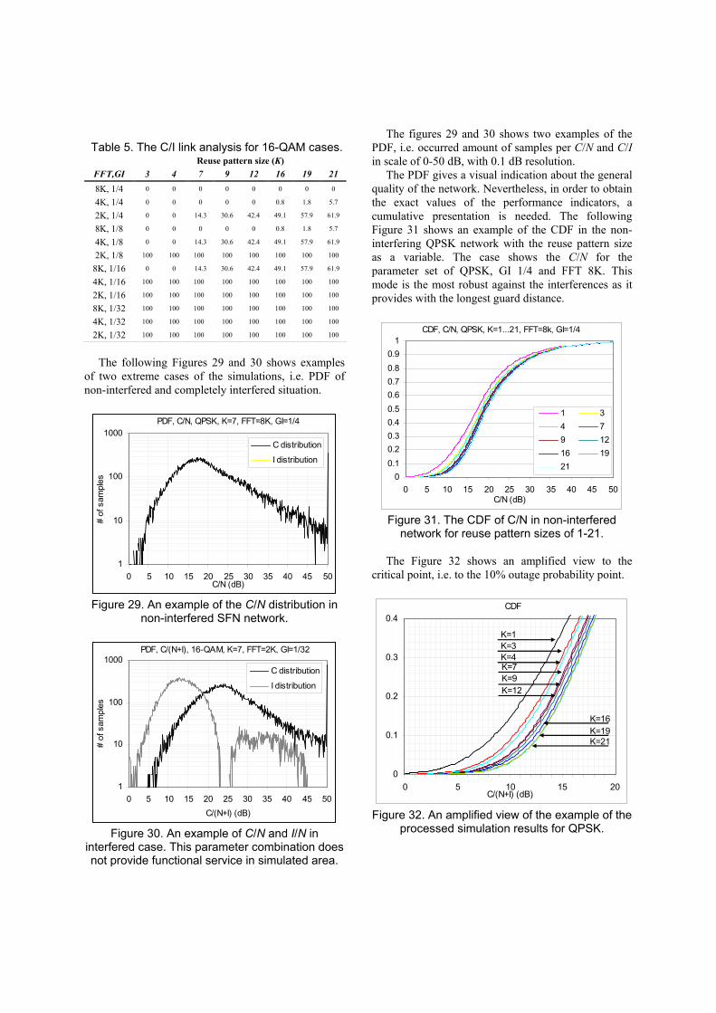
The following Figures 29 and 30 shows examples

of two extreme cases of the simulations, i.e. PDF of non-interfered and completely interfered situation.

PDF, C/N, QPSK, K=7, FFT=8K, GI=1/4

1

10

100

1000

0 5 10 15 20 25 30 35 40 45 50C/N (dB)

# of

sam

ples

C distribution

I distribution

Figure 29. An example of the C/N distribution in

non-interfered SFN network.

PDF, C/(N+I), 16-QAM, K=7, FFT=2K, GI=1/32

1

10

100

1000

0 5 10 15 20 25 30 35 40 45 50C/(N+I) (dB)

# of

sam

ples

C distribution

I distribution

Figure 30. An example of C/N and I/N in

interfered case. This parameter combination does not provide functional service in simulated area.

The figures 29 and 30 shows two examples of the PDF, i.e. occurred amount of samples per C/N and C/I in scale of 0-50 dB, with 0.1 dB resolution.

The PDF gives a visual indication about the general quality of the network. Nevertheless, in order to obtain the exact values of the performance indicators, a cumulative presentation is needed. The following Figure 31 shows an example of the CDF in the non-interfering QPSK network with the reuse pattern size as a variable. The case shows the C/N for the parameter set of QPSK, GI 1/4 and FFT 8K. This mode is the most robust against the interferences as it provides with the longest guard distance.

CDF, C/N, QPSK, K=1...21, FFT=8k, GI=1/4

00.10.20.30.40.50.60.70.80.9

1

0 5 10 15 20 25 30 35 40 45 50C/N (dB)

1 34 79 1216 1921

Figure 31. The CDF of C/N in non-interfered

network for reuse pattern sizes of 1-21. The Figure 32 shows an amplified view to the

critical point, i.e. to the 10% outage probability point.

CDF

0

0.1

0.2

0.3

0.4

0 5 10 15 20C/(N+I) (dB)

K=1K=3K=4K=7K=9K=12

K=16K=19K=21

Figure 32. An amplified view of the example of the

processed simulation results for QPSK.

Table 5. The C/I link analysis for 16-QAM cases. Reuse pattern size (K)

FFT,GI 3 4 7 9 12 16 19 21 8K, 1/4 0 0 0 0 0 0 0 0

4K, 1/4 0 0 0 0 0 0.8 1.8 5.7

2K, 1/4 0 0 14.3 30.6 42.4 49.1 57.9 61.9

8K, 1/8 0 0 0 0 0 0.8 1.8 5.7

4K, 1/8 0 0 14.3 30.6 42.4 49.1 57.9 61.9

2K, 1/8 100 100 100 100 100 100 100 100

8K, 1/16 0 0 14.3 30.6 42.4 49.1 57.9 61.9

4K, 1/16 100 100 100 100 100 100 100 100

2K, 1/16 100 100 100 100 100 100 100 100

8K, 1/32 100 100 100 100 100 100 100 100

4K, 1/32 100 100 100 100 100 100 100 100

2K, 1/32 100 100 100 100 100 100 100 100

As can be seen form the Figure 32, the single cell (K=1) results a minimum of 8.5 dB for the 10 % outage probability, i.e. for the area location probability of 90% in the whole cell area which corresponds to the 70% area location probability in the cell edge. The cell is thus correctly dimensioned for the simulations.

In order to find the respective SFN gain level, the comparison with single cell and other reuse pattern sizes can be made in this 10% outage point. The following Figures 33 and 34 shows the respective simulation results for all the symmetrical reuse pattern sizes 1-21 for QPSK and 16-QAM.

SFN gain, QPSK

-15.0

-10.0

-5.0

0.0

5.0

1 3 4 7 9 12 16 19 21

K

SFN

gai

n (d

B)


Figure 33. The SFN gain levels for QPSK cases,

with the reuse pattern sizes of 1-21.

SFN gain, 16-QAM

-20.0

-15.0

-10.0

-5.0

0.0

5.0

1 3 4 7 9 12 16 19 21

K

SFN

gai

n (d

B)


Figure 34. The SFN gain levels for 16-QAM cases, with the reuse pattern sizes of 1-21.

The simulation results show the level of SFN gain.

The reference case FFT 8K and GI ¼ results the maximum gain for the reuse pattern sizes of K=1-21 for both QPSK and 16-QAM and provides a non-interfering network. In addition, the parameter set of FFT = 4K, GI = 1/4 and FFT = 8K, GI = 1/8

results a network where SFN errors can be compensated with the SFN gain.

According to the results shown in Figure 33, the QPSK case could provide SFN gain of 3-4 dB in non-interfering network. It is interesting to note that in the interfering cases, also the parameter set of GI = ¼, FFT = 4K corresponding FFT = 8K, GI = 1/8 results positive SFN gain even with the interference present for all the reuse pattern cases up to 21. Also the parameter set of GI = ¼, FFT = 2K, corresponding FFT = 8K, GI = 1/16 and FFT = 4K, GI = 1/8 provides an adequate quality level until reuse pattern of 16 although the error level (SER) increases.

According to the Figure 34, the 16-QAM gives equal SFN gain, resulting about 3-4 dB in non-interfering network. For the FFT = 4K, GI = ¼ and the corresponding parameter set of FFT = 8K, GI = 1/8, the SFN gain is higher than the SER even with higher reuse pattern sizes compared to QPSK, because the 16-QAM cell size is smaller.

As can be seen from the Figures 33-34 and from the C/I link analysis of Tables 4-5, the rest of the cases are practically useless with the selected parameter set. 6. Methodology for the simulations: third variation (urban SFN network) 6.1. Simulation environment

The dense and urban area of Mexico City was used

as a basis for the next simulations by applying suitable propagation prediction models (Okumura-Hata and ITU-R P.1546-3). The city is located on relatively flat ground level with high mountains surrounding the centre area which was taken into account in the radio interface modelling.

The height of the planned DVB-H site antennas was 60, 190, 30, 20, 20, 30 and 30 meters from the tower base, respectively for the sites 1-7. The site number 7 represents the mountain installation with the tower base located 800 meters above the average ground level which results the effective antenna height of 860 meters compared to the city centre level. Site number 4 is also situated in relatively high level, but in this case, the surrounding area of the site limits its coverage area. The rest of the sites are located in the base level of Mexico City centre.

As the cell radius of the investigated sites is clearly smaller than 20 km, the Okumura-Hata [3] is suitable for the path loss prediction for all the other sites except for the mountain site number 7. The Figure 38 shows the principle of the geographical profile of this site, varying the horizontal angle from the site to the centre

by 10 degree steps. As the profile shows, there are smaller mountains found in front of the site.

urban

dense urban

forest

open

residential

4 8 12 16 20km 4 8 12 16 20km

Figure 35. The clutter type of the investigated

area.

Figure 36. The predicted coverage area of the

investigated network as analyzed with a separate radio network planning tool.

The Figure 37 presents the location of the selected sites, and the Table 6 shows the site parameters.

For the site number 7, ITU-R P.1546 (version 3) [2] model was applied by using the antenna height of 860 meters and frequency of 680 MHz.

The calculation of the path loss for the site number 7 was done in practice by interpolating the correct ITU-R P.1546 curve for 860 meter antenna height (via 600 and 1200 meter heights) and for 680 MHz

frequency (via 600 and 2000 MHz). The Figure 39 shows the resulting curve after the iterations.

Geographical site location

0

10

20

30

40

0 10 20 30 40 km

km

1

23

45

6

7

Figure 37. The site locations and informative

relative site sizes of the simulator.

Terrain height profile Tres Padres - Center

2200

2300

2400

2500

2600

2700

2800

2900

3000

0.0

1.0

2.0

3.0

4.0

5.0

6.0

7.0

8.0

9.0

10.0

11.0

12.0

13.0

14.0

15.0

16.0

17.0

Distance (km)

Terr

ain

heig

ht (m

from

sea

leve

l)

Height 1 (TP-Zocalo)Height 2 (TP-Chapultepec)Height 3 (TP-middle)

Figure 38. The profile of the mountain site 7.

Path loss

110

120

130

140

150

160

170

180

190

200

1 2 3 4 5 6 7 8 9 10 11 12 13 14 15 16 17 18 19 20 30 40 50 60 70 80 90

Distance (km)

L (d

B)

6008601200FSL

Figure 39. The estimated path loss L for the

mountain site. FSL is free space loss reference.

Next, a trend line was created in order to present the tabulated values with a closed formula and to ease the simulations. For this specific case, there was one formula created for the path loss in distances of 1-20 km (L20) and another one for the distances of 20-100 km (L100), d being the distance (km):

84.113)ln(659.1020 += dL (18)

55.1355124.0100 += dL (19)

In order to estimate the error between the trend

lines and the original ITU-model, the following Figure 40 was produced. In the functional area of the mountain site, the maximum error is < 0.5 dB.

Difference of trend line and original values

-1.0-0.8-0.6-0.4-0.20.00.20.40.60.81.0

1 2 3 4 5 6 7 8 9 10 11 12 13 14 15 16 17 18 19 20 30 40 50 60 70 80 90

Distance (km)

Diff

(reg

ress

ion

- orig

inal

)

Figure 40. The estimated error margin for the

trend lines used for the mountain site path loss calculation.

The link budget of the simulator takes into account

separately the radiating power levels and antenna heights of each site as seen in Table 6.

During the simulations, the receiver was placed

randomly in the investigated area (45km × 45km = 2025 km2) according to the snap-shot principle and uniform geographical distribution. In each simulation

round, the separate sum of the carrier per noise and the interference per noise was calculated by converting the received power levels into absolute powers. The result gives thus information about the balance of SFN gain and SFN interference levels. Tables of geographical coordinates with the respective sum of carriers and interferences were created by repeating the simulations 60,000 times. Also carrier and interference level distribution tables were created with a scale of -50 … +50 dB.

The long-term as well as Rayleigh fading was taken into account in the simulations by using respective distribution tables independently for each simulation round. A value of 5.5 dB was used for the standard deviation. The area location probability in the cell edge of 90% was selected for the quality criteria, producing about 7 dB shadowing margin for the long-term fading. Terminal antenna gain of -7.3 dBi was used in the calculations according to the principles indicated in [1]. Terminal noise figure of 5 dB was taken into account. Both Code Rate and MPE-FEC Rate were set to ½.

6.2. Simulation results

The usable coverage area was investigated by post-

processing the simulation results. The simulations were carried out by using QPSK and 16-QAM modulations, CR ½, MPE-FEC ½ and all the possible variations of FFT and GI.

Figure 41. Example of the non-interfered network with the parameter setting of QPSK, GI=1/4 and

FFT = 8k. As expected, the parameter set of QPSK, FFT 8k,

GI 1/4 produces the largest coverage area practically without interferences (Figure 41). The results of this

Table 6. The site parameters. Site Coord., km EIRP Radius, km

nr x y dBm W QPSK 16-QAM

1 7.2 11.0 70.5 11258 4.1 2.8 2 19.0 4.4 69.3 8481 5.6 3.8 3 20.5 5.8 69.3 8481 4.6 3.2 4 26.4 12.7 69.5 8860 5.0 3.4 5 21.2 16.1 71.3 13411 15.5 9.8 6 16.6 27.0 69.3 8481 5.0 3.4 7 23.0 36.4 71.1 12837 26.3 15.8

case can be considered thus as a reference for the interference point of view.

When the GI and FFT values are altered, the level of interference varies respectively. The results show that in addition to the parameter set of FFT 8k, GI1/4, also FFT 8k, GI 1/8, FFT 4k, GI 1/4 produces useful coverage areas, i.e. the balance of the SFN gain and SFN interferences seem to be in acceptable levels, whilst the other parameter settings produces highly interfered network.

The 16-QAM produces smaller coverage areas compared to the QPSK as the basic requirement for the C / (N + I) of 16-QAM is 14.5 dB instead of the 8.5 of QPSK.

Figure 42. Comparative example of the simulation results for the parameter set of 16-QAM, FFT 8k

and GI 1/16. As can be observed from the previous analysis and

Figure 42, the SFN interferences tend to cumulate to the outer boundaries of the planned coverage area.

For the QPSK with FFT 8k and GI ¼, the area is practically free of interferences, i.e. the C / (N + I) is > 8.5 dB in every simulated location. The dark colour in the middle shows the site locations with the C / (N + I) greater than 35 dB.

By observing the 90% probability in the cell edge (about 95% in the cell area), i.e. 5 % outage probability of the Figures 43-44, the mode FFT 8k, GI1/4 provides a minimum of about 7 dB and the set of FFT 8k, GI1/8 and FFT 4k, GI1/4 provides the same performance in the whole investigated area. This similarity is due to the Dsfn limit, which is complied totally in both of the cases as the sites are grouped inside about 30 km diameter. It is worth noting that the values are calculated over the whole map of 45km × 45km.

CDF, C/(N+I)

0

0.10.2

0.3

0.40.5

0.6

0.7

0.80.9

1

-50 -40 -30 -20 -10 0 10 20 30 40 50C/(N+I), dB

QPSK, FFT 8k, GI 1/4QPSK, FFT 8k, GI 1/8QPSK, FFT 8k, GI 1/16QPSK, FFT 8k, GI 1/32QPSK, FFT 4k, GI 1/32QPSK, FFT 2k, GI 1/32

Figure 43. The cumulative C/(N+I) distribution of

different modes for QPSK.

CDF, C/(N+I)

0

0.1

0.20.3

0.4

0.5

0.6

0.70.8

0.9

1

-50 -40 -30 -20 -10 0 10 20 30 40 50C/(N+I), dB

16-QAM , FFT 8k, GI 1/416-QAM , FFT 8k, GI 1/816-QAM , FFT 8k, GI 1/1616-QAM , FFT 8k, GI 1/3216-QAM , FFT 4k, GI 1/3216-QAM , FFT 2k, GI 1/32

Figure 44. The cumulative C/(N+I) distribution of

different modes for 16-QAM.

Area-% for C/(N+I) >= 8.5 dB

0

10

20

30

40

50

60

70

80

90

100

QPSK,8k,1/

4

QPSK,8k,1/

8

QPSK,8k,1/

16

QPSK,8k,1/

32

QPSK,4k,1/

32

QPSK,2k,1/

32

Figure 45. The functional area percentage for

QPSK modes compared to the total area.

Area-% for C/(N+I) >= 14.5 dB

0

10

20

30

40

50

60

70

80

90

100

16-Q

AM,8k,1/

4

16-Q

AM,8k,1/

8

16-Q

AM,8k,1/

16

16-Q

AM,8k,1/

32

16-Q

AM,4k,1/

32

16-Q

AM,2k,1/

32

Figure 46. The functional area percentage for 16-

QAM modes compared to the total simulated area.

It seems that the QPSK mode would provide a good

performance in the investigated area when using the non-interfering FFT 8k, GI 1/4 parameters, whilst 16-QAM gives smaller yet non-interfered coverage area. The advantage of the latter case is the double radio channel capacity compared to the QPSK with greater coverage area. The parameter set of FFT 8k, GI 1/8 and FFT 4k, GI 1/4 looks also useful, providing the possibility to either rise the maximum velocity of the terminal (FFT 4k), or give more capacity (GI 1/8). As for the rest of the parameter settings, the optimal balance can not be achieved due to the raised interference levels.

The SFN gain of the investigated network could be observed more specifically by switching on and off the individual sites, by carrying out the C / (N + I) simulations and by noting the differences in the cumulative density function. This is not, though, accurate method unless the simulations are limited inside the maximum calculated cell radius of each site. The network layout used in this case is highly irregular and does not contain too much overlapping areas compared to the total area of 45 km × 45 km, so the separate SFN gain investigation was not carried out. On the other hand, the presented results already include the total sum of the SFN gain and interference.

It can be estimated though that especially with the QPSK modes that provides with the largest coverage areas, the mountain site does have an effect within the overlapping areas of the nearest cells. According to the simulations presented in Figure 33, this case could provide an SFN gain of about 1 dB in such areas. Similarly, if there is spot with three overlapping cells in the middle of the area (i.e. in the area without interferences), the SFN gain could be around 2 dB

according to the simulations presented in the chapter showing the balance of the SFN gain and SFN interferences. The results presented in e.g. [9] support this observation. 7. Conclusions

The presented simulation method provides both geographical and cumulative distribution of the SFN gain and interference levels. The method takes into account the balancing of the coverage and capacity as well as the optimal level of SFN gain and the interference level in case the over-sized SFN is used. It can be applied for the theoretical, e.g. hexagonal cell layouts, as well as for the practical environments, taking into account the radio propagation modelling for different sites.

The method can thus be used in the detailed optimization of the DVB-H networks. The principle of the simulator is relatively straightforward and the method can be applied by using various different programming languages. In these investigations, a standard Pascal was used for programming the core simulator.

The SFN gain results are in align with the practical results of e.g. [5] and [9] for the low number site. For the high number of the sites, no reference results were found due to the practical challenges in setting up the test cases. Nevertheless, estimating the theoretical limits by applying the formula [5], the results are in logical range. The SFN interference level results behave also logically and are in align with e.g. [12].

The results show that the radio parameter selection is essential in the detailed planning of the DVB-H network. As the graphical presentation of the results indicate, the effect of the parameter value selection on the interference level and thus on the quality of service can be drastic, which should be taken into account in the detailed planning of DVB-H SFN.

Especially the controlled extension of the SFN limit might be interesting option for the DVB-H operators. The simulation method and related results shows logical behaviour of the SFN error rate when varying the essential radio parameters. The results also show that the optimal setting can be obtained using the respective simulation method by balancing the SFN gain and SFN errors. As expected, the 8K mode is the most robust when extending the SFN whilst 4K limits the maximum site antenna height. 16-QAM provides suitable performance for the extension, but according to the results, even QPSK which provides larger coverage areas is not useless in SFN extension when selecting the parameters correctly.

8. References [1] DVB-H Implementation Guidelines. Draft TR 102 377 V1.2.2 (2006-03). European Broadcasting Union. 108 p. [2] Jukka Henriksson. DVB-H standard, principles and services. HUT seminar T-111.590. Helsinki, 24.2.2005. Presentation material. 53 p. [3] Editor: Thibault Bouttevin. Wing TV. Services to Wireless, Integrated, Nomadic, GPRS-UMTS&TV handheld terminals. D8 – Wing TV Measurement Guidelines & Criteria. Project report. 45 p. [4] Editor: Maite Aparicio. Wing TV. Services to Wireless, Integrated, Nomadic, GPRS-UMTS&TV handheld terminals. D6 – Wing TV Common field trials report. Project report, November 2006. 86 p. [5] Editor: Maite Aparicio. Wing TV. Services to Wireless, Integrated, Nomadic, GPRS-UMTS&TV handheld terminals. D8 – Wing TV Country field trial report. Project report, November 2006. 258 p. [6] Editor: Davide Milanesio. Wing TV. Services to Wireless Integrated, Nomadic, GPRS-UMTS&TV handheld terminals. D11 – WingTV Network Issues. Project report, May 2006. 140 p. [7] Gerard Faria, Jukka A. Henriksson, Erik Stare, Pekka Talmola. DVB-H: Digital Broadcast Services to Handheld Devices. IEEE 2006. 16 p. [8] William C.Y. Lee. Elements of Cellular Mobile Radio System. IEEE Transactions on Vehicular Technology, Vol. VT-35, No. 2, May 1986. pp. 48-56. [9] David Plets. New Method to Determine the SFN Gain of a DVB-H Network with Multiple Transmitters. 58th Annual IEEE Broadcast Symposium, 15-17 October 2008, Alexandria, VA, USA. 6 p. [10] Masaharu Hata. Empirical Formula for Propagation Loss in Land Mobile Radio Services. IEEE Transactions on Vehicular Technology, Vol. VT-29, No. 3, August 1980. 9 p. [11] Recommendation ITU-R P.1546-3. Method for point-to-area predictions for terrestrial services in the frequency range 30 MHz to 3000 MHz. 2007. 57 p.

[12] Airi Silvennoinen. DVB-H –lähetysverkon opti-mointi Suomen olosuhteissa (DVB-H Network Optimi-zation under Finnish Conditions). Master’s Thesis, Helsinki University of Technology, 15.5.2006. 111 p. [13] Jyrki T.J. Penttinen. The Simulation of the Interference Levels in Extended DVB-H SFN Areas. The Fourth International Conference on Wireless and Mobile Communications. IEEE 2008. Pp. 223-228. [14] Jyrki T.J. Penttinen. The SFN gain in non-interfered and interfered DVB-H networks. The Fourth International Conference on Wireless and Mobile Communications. IEEE 2008. Pp. 294-299. [15] Jyrki T.J. Penttinen. DVB-H Performance Simulations in Dense Urban Area. The Third International Conference on Digital Society. IEEE 2009. 6 p. [16] Minseok Jeong. Comparison Between Path-Loss Prediction Models for Wireless Telecommunication System Design. IEEE, 2001. 4 p. Biography

Mr. Jyrki T.J. Penttinen has worked in telecommunications area since 1994, for Telecom Finland and it’s successors until 2004, and after that, for Nokia and Nokia Siemens Networks. He has carried out various international tasks, e.g.

as a System Expert and Senior Network Architect in Finland, R&D Manager in Spain and Technical Manager in Mexico and USA. He currently holds a Senior Solutions Architect position in Madrid, Spain. His main activities have been related to mobile and DVB-H network design and optimization.

Mr. Penttinen obtained M.Sc. (E.E.) and Licentiate of Technology (E.E.) degrees from Helsinki University of Technology (TKK) in 1994 and 1999, respectively. He has organized actively telecom courses and lectures. In addition, he has published various technical books and articles since 1996. His main books are “GSM-tekniikka” (“GSM Technology”, published in Finnish, Helsinki, Finland, WSOY, 1999), “Wireless Data in GPRS” (published in Finnish and English, Helsinki, Finland, WSOY, 2002) and “Tietoliikennetekniikka” (“Telecommunications tech-nology”, published in Finnish, Helsinki, Finland, WSOY, 2006).

publication i “capex and opex optimisation in function of ... · pdf...

Documents