estimating opex and capex efficiency - · pdf fileestimating opex and capex efficiency a final...

July 2004

ESTIMATING OPEX AND CAPEX EFFICIENCY A Final Report for Water UK

Project Team

Bill Baker James Grayburn Paul Metcalfe Anna Navidski

NERA Economic Consulting 15 Stratford Place London W1C 1BE United Kingdom Tel: +44 20 7659 8500 Fax: +44 20 7659 8501 www.nera.com

Contents

NERA Economic Consulting

i

Contents

Contents ........................................................................................................................................... i

List of Figures ................................................................................................................................ iii

List of Tables ................................................................................................................................. iv

Executive Summary ......................................................................................................................... i

I. Introduction..........................................................................................................................1

II. Background and Approach ..................................................................................................2 A. Previous Work and Best Practice.........................................................................................2 B. Our Approach.......................................................................................................................3 C. Defining Terms ....................................................................................................................3

III. Top-down TFP Estimates ....................................................................................................5 A. Summary of estimates..........................................................................................................5 B. Estimating Baseline TFP......................................................................................................7 C. Adjusting Baseline TFP Estimates for Quality....................................................................8 D. Adjusting TFP Estimates for Privatisation Effect..............................................................10 E. Summary of TFP Estimates for Water and Sewerage Sector ............................................11 F. Estimating Economy-Wide TFP........................................................................................12 G. Conclusions on “Net TFP”.................................................................................................13

IV. Top-Down Non-capital and Capital PFP ...........................................................................14 A. Capital and Non-Capital PFP.............................................................................................14 B. Deriving Consistent PFPs ..................................................................................................16

V. Bottom-up TFP Estimates..................................................................................................18 A. LE’s Bottom-up Approach.................................................................................................18 B. Comparing LE’s Top-down and Bottom-up Estimates .....................................................19 C. Babtie Report on Cost Saving Technologies .....................................................................20 D. Conclusions on Bottom-up Approach to Estimating TFP .................................................21

VI. Forecasting Relative Input Price Changes .........................................................................22 A. Opex Input Price Forecasts ................................................................................................22 B. Capex Input Price Forecasts...............................................................................................25 C. Water Sector Input Prices ..................................................................................................25 D. Whole Economy Input Prices ............................................................................................26 E. Conclusions on Input Price Effects....................................................................................26

VII. Setting X: Conclusions ......................................................................................................28 A. Estimating X ......................................................................................................................28 B. Setting Xcapex and Xopex.................................................................................................30

Contents


ii

Appendix A. Some Proposals for an Agreed Methodology for setting EffIciency..............32

Appendix B. Water sector TFP Estimates............................................................................33

Appendix C. Economy-Wide TFP Estimates.......................................................................37

Appendix D. Deriving Capital Efficiency From TFP ..........................................................40

Appendix E. Estimating Water and Sewerage Sector Input Prices .....................................41 E.1. Labour Prices ...............................................................................................................41 E.2. Power Prices.................................................................................................................43 E.3. Materials Prices............................................................................................................46 E.4. Governmental Charges.................................................................................................48 E.5. CAPEX Prices..............................................................................................................50

Appendix F. Deriving Economy-Wide Input Price Forecasts .............................................54

Appendix G. TFP estimates For a Range of Economic Sectors...........................................56

Appendix H. Anticipated Input Price Changes and RPI ......................................................57

List of Figures


iii

List of Figures

Figure E.1 Real Earnings Growth (various indices) (per cent per year) 42

Figure E.2 Real Industrial Electricity Price Index (1990=100)1 44

Figure E.3 Real Materials Price Indices 47

Figure E.4 Real Materials Prices (Combined Electricals and Chemicals Index, 1991=100) 48

Figure E.5 COPI and RPIX Annual Inflation (per cent per year) 51

Figure E.6 COPI Inflation Relative to RPI (per cent per year) 52

List of Tables


iv

List of Tables

Table 3.1 Summary of TFP Estimates 6

Table 3.2 Water and Sewerage Quality Adjustments to TFP 9

Table 3.3 Economy-wide TFP Estimates 13

Table 3.4 Relative TFP Growth for Water and Sewerage Sector, 2005-10 13

Table 4.1 Non-capital PFP Estimates 15

Table 4.2 Capital PFP Estimates 16

Table 5.1 LE's Top-down and Bottom-up Results 19

Table 5.2 Summary of Likely Capital Cost Savings 2000-05 as Identified by Babtie 21

Table 6.1 Nominal Opex Input Price Forecasts 25

Table 6.2 Water Sector Nominal Input Price Projection 26

Table 6.3 Nominal Opex Input Price Forecasts (whole economy) 26

Table 6.4 Relative Input Price Forecast, 2005-2010 27

Table 7.1 Derivation of X (% p.a.) 30

Table B.1 Current Water Sector TFP Estimates (% per annum) 33

Table C.1 Whole Economy TFP Estimates (% per annum) 37

Table E.1 Labour Price Indices 41

Table E.2 Central Forecasts for UK Average Earnings Growth 43

Table E.3 Retail Price Scenarios for UK Electricity Supplies 44

Table E.4 DNO Forecasts for 2005-10 Distribution Costs (percentage change 2005-10 over 2000-05)45

Table E.5 Materials Price Indices 46

Table E.6 Forward View of Real Construction Price Growth 53

Table F.1 ONS Indices Used to Obtain Weights in Opex Price Forecast 54

Table F.2 OEF Manufacturing Producer Input Prices Forecast (Nominal, % Change per Year) 54

Table F.3 OEF Manufacturing Producer Output Prices Forecast (Nominal, % Change per Year) 55

Table G.1 Sector Level TFP Estimates (CAGR %) 56

Executive Summary

i

Executive Summary

This report estimates the scope for opex and capex efficiency for the water industry over the period 2005-2010, building upon the recent study undertaken by London Economics (LE) for Ofwat, and also referencing recent reports by Europe Economics (EE, again, for Ofwat), Cambridge Economic Policy Associates (CEPA, for Ofgem) and other studies.1 In this study, following convention in the academic literature, we use the term “efficiency” as equivalent to the term “unit costs”. We note that the expected change in efficiency is a combination of two factors: the expected change in productivity and the expected change in input prices. The change in productivity is a measure of the change in outputs relative to inputs. Typically, sector and economy-wide productivity is positive because of, for example, innovation, which results in an increase in outputs relative to the required inputs. However, potential efficiency gains from productivity are offset by increases in input prices. Depending on the relative size of input price effects, efficiency can therefore be positive (i.e. unit cost reduction) or negative (i.e. unit cost increase). In estimating efficiency, we set out estimates of productivity improvements and input price changes separately. Our approach is consistent with the academic literature on allowing for anticipated efficiency change (or “X”) in an indexed (“RPI”) price-cap regime, where the expected change in unit costs is set equal to sector level productivity improvements minus input price changes, where both productivity and input prices are measured relative to whole-economy effects.

Estimating Total Factor Productivity

Our estimates of total factor productivity (TFP) growth for the UK water and sewerage sector relative to whole-economy effects are based on empirical work from other studies. TFP growth is a measure of the growth rate of total outputs of a company, sector or economy relative to the growth rate of the required level of inputs. In measuring water service TFP growth, total water delivered is commonly used as the measure of outputs for the water sector, and sewage volume collected adjusted for leads is generally the sewerage service output. The inputs comprise operating expenditures (mainly labour, materials and energy) and total capital services. TFP growth can be measured on the basis of top-down or bottom-up approaches. Top-down approaches to TFP growth use aggregate level industry (or comparator sector) data, whereas bottom-up approaches attempt to estimate TFP on the basis of disaggregated data, e.g. by focusing on the expected change in individual components of companies’ costs. In this report, we disregard the evidence from bottom-up approaches because we do not consider these estimates to be robust in the studies to date.

1 London Economics, Black & Veatch Consulting and Prof. M.F. Shutler (LSE) (2003), PR04 Scope for

Efficiency Studies, Final Report to Ofwat; Europe Economics (2003), Scope for Efficiency Improvement in the Water and Sewerage Industries, Final Report to Ofwat; Cambridge Economic Policy Associates(2003), Productivity improvements in distribution network operators, Final Report to Ofgem

Executive Summary

ii

In the water sector, one key difficulty with measuring TFP is the adjustment required to the measure of outputs to capture improvements in water and wastewater service quality (e.g. improvements in drinking quality standards). If we do not adjust for quality changes, we will underestimate the historic improvements in TFP because our output figure, measured in physical quantities, will underestimate the true value of output. In estimating anticipated changes in England and Wales water sector TFP from historic data, we also have to adjust for the transitory nature of any relatively higher levels of productivity growth secured immediately post-privatisation. We first set out our best estimate for “baseline” TFP growth in the water sector, which we define as TFP growth prior to adjustments for quality and privatisation effects. In estimating TFP, we disregard evidence from comparator sector approaches, which we believe provide less robust estimates of water and sewerage sector TFP. Instead we draw on empirical studies that use water and sewerage sector level data; these comprise the recent study by LE for Ofwat, CEPA for Ofgem, and an academic paper by Saal and Parker.2 These three studies estimate baseline TFP to be in the range of –0.6% to +0.5% per year. We therefore consider a reasonable estimate of “baseline” TFP growth over the period 1990-2000 (the approximate period of these three studies) to be 0% per year. From this baseline estimate, we then consider two potential adjustments: for quality, and for the transitory privatisation effect. Our referenced studies make very different adjustments to the measured level of outputs and their baseline TFP measure to reflect quality improvements. LE and S&P’s adjustment for quality is based on the proportion of water zones that comply with Ofwat’s DG service measures, borrowing the approach developed by S&P in their 2001 study. This approach increases the baseline TFP figure by approximately +0.7% for LE and +1.9% for S&P. CEPA uses “quality enhancement weighted” and “customer willingness to pay” weighted quality adjustments, which suggest very different upward revisions of +6.2% and +0.3% respectively. Our survey suggests that there is as yet no clearly accepted adjustment for quality, and that all the applications to date involve substantial subjectivity. In the absence of a clearly superior approach, and noting that a future decrease and/or change in composition of the quality programme might reduce the scope for companies to secure future productivity improvements in this way, we take a conservative approach and adopt the mid-point of the two lower estimates: CEPA’s “customer willingness to pay” approach which suggest an upward adjustment of +0.3%, and LE’s adjustment for quality of approximately +0.7%. This leads us to an upward adjustment to our baseline TFP figure for quality of +0.5%. Therefore, we conclude that the most reasonable estimate for quality adjusted TFP growth in the water and sewerage sector (prior to an adjustment for the privatisation effect) is +0.5%. Because our preferred estimate of +0.5% is based on evidence from E&W in 1990-2000, it implicitly incorporates any privatisation effect from E&W over this period. We consider that any transitory gains from privatisation will be substantially eroded by the period 2005-2010,

2 LE (2004) op. cit; CEPA (2004) op. cit.; Saal and Parker (2001), Productivity and Price Performance in the

Privatised Water and Sewerage Companies of England and Wales.

Executive Summary

iii

more than fifteen years following privatisation. Our survey demonstrates that there is no clear consensus on the initial size and subsequent diminution of the privatisation effect. In the absence of a clear consensus, we shade-down our estimate of the anticipated TFP growth rate by a conservative +0.1% to +0.4%. The next step is to establish the anticipated change in economy wide TFP. We prefer long-run estimates of economy-wide TFP because TFP measures over the short-run can be influenced by the economic cycle. Estimates for the economy-wide TFP growth, based on long term historic estimates post-1970s oil crisis, are clustered around +1.3%. We consider the historic TFP growth rate of +1.3% as the best indicator of economy-wide TFP over the next review period. We therefore estimate a water sector TFP growth rate relative to the whole economy of +0.4% minus +1.3%, or –0.9% p.a. (see Table 1).

Table 1

Derivation of Water and Sewerage Sector TFP Growth Relative to the Whole Economy

Step % per year

a. “Baseline” TFP estimate 0% b. Quality adjustment +0.5% c. Privatisation effect adjustment -0.1% d. Quality adjusted TFP (=a+b+c) +0.4% e. Economy-wide TFP estimate +1.3% f. Relative TFP estimate (=d-e) -0.9% Source: NERA analysis and review of referenced studies.

Estimating Partial Factor Productivities

Partial factor productivity (PFP) is a measure of the rate of change of output relative to a single input. PFPs will differ from TFP to the extent that there are differential growth rates in the use of different inputs. All of our referenced studies demonstrate that opex (or a labour proxy) PFP has been greater than capital PFP in the water and sewerage sector, which equates to the general understanding that capital inputs have increased at a greater rate (or have declined at a lower rate) than opex inputs. In deriving anticipated capital and non-capital PFP for the period 2005-2010, we also have to consider the possible diminution of capital substitution. We would expect the water industry to experience a greater rate of factor substitution immediately post-privatisation (when the water companies were freed of public capital expenditure limits), and therefore we would expect the differential growth rates in the future to be lower than historic outturn differentials. To derive PFPs consistent with our TFP estimate, we make the simplifying assumption that capital PFP is approximately +0.4% lower than our TFP estimate of +0.4%, that is 0% p.a.

Executive Summary

iv

(i.e. capital services keep pace with output). This is based on evidence from our referenced studies, notably CEPA. We then derive a PFP for opex of +1%, consistent with our estimate of 0% for capital PFP and the input shares. However, we consider that our overall estimate of +0.4% for TFP is more robust than our estimates of 0% and 1% for capital and non-capital (opex) PFPs. This is because there is more evidence supporting our TFP figure, whereas there is relatively disparate evidence for PFPs in our referenced studies.

Estimating Input Price Effects

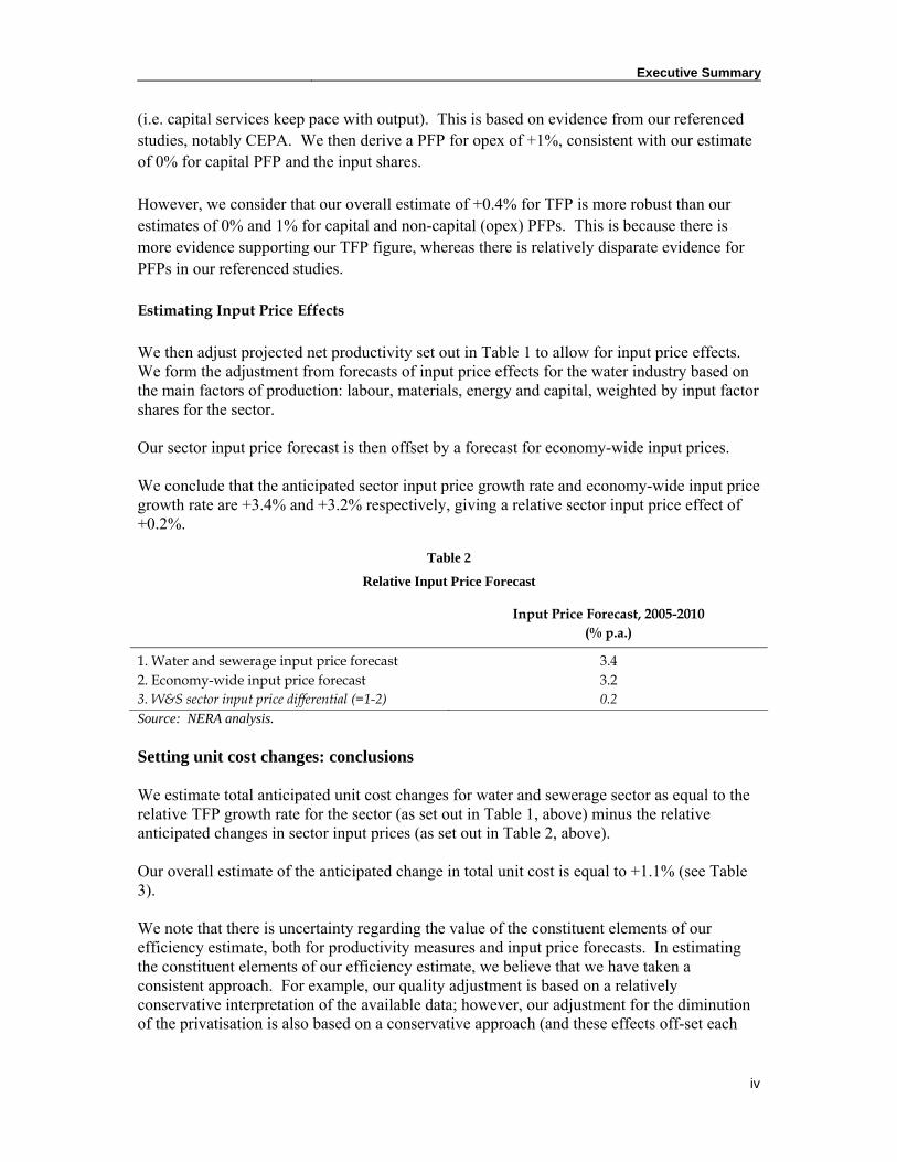
We then adjust projected net productivity set out in Table 1 to allow for input price effects. We form the adjustment from forecasts of input price effects for the water industry based on the main factors of production: labour, materials, energy and capital, weighted by input factor shares for the sector. Our sector input price forecast is then offset by a forecast for economy-wide input prices. We conclude that the anticipated sector input price growth rate and economy-wide input price growth rate are +3.4% and +3.2% respectively, giving a relative sector input price effect of +0.2%.

Table 2

Relative Input Price Forecast

Input Price Forecast, 2005-2010 (% p.a.)

1. Water and sewerage input price forecast 3.4 2. Economy-wide input price forecast 3.2 3. W&S sector input price differential (=1-2) 0.2 Source: NERA analysis. Setting unit cost changes: conclusions We estimate total anticipated unit cost changes for water and sewerage sector as equal to the relative TFP growth rate for the sector (as set out in Table 1, above) minus the relative anticipated changes in sector input prices (as set out in Table 2, above). Our overall estimate of the anticipated change in total unit cost is equal to +1.1% (see Table 3). We note that there is uncertainty regarding the value of the constituent elements of our efficiency estimate, both for productivity measures and input price forecasts. In estimating the constituent elements of our efficiency estimate, we believe that we have taken a consistent approach. For example, our quality adjustment is based on a relatively conservative interpretation of the available data; however, our adjustment for the diminution of the privatisation is also based on a conservative approach (and these effects off-set each

Executive Summary

v

other). Therefore, we believe our final unit cost estimate of 1.1% is based on a consistent set of parameters.

Table 3

Derivation of Anticipated Total Unit Cost Change or X (% p.a.)

Step % per year

a. “Baseline” TFP estimate 0% b. Quality adjustment +0.5% c. Privatisation effect adjustment -0.1% d. Quality adjusted TFP (=a+b+c) +0.4% e. Economy-wide TFP estimate +1.3% f. Relative TFP estimate (=d-e) -0.9% g. Water sector input prices adjustment +3.4% h. Economy-wide input prices adjustment +3.2% i. “X” (=f-(g-h)) -1.1% j. Anticipated real change in unit costs (=-i) +1.1% Source: NERA analysis and review of referenced studies.

We do not estimate separate unit cost changes for operating (Xopex) and capital expenditure cost lines (Xcapex). We consider that our estimate of overall efficiency savings (“X”) is more robust. This is because there is relatively disparate evidence on the capital and non-capital PFPs, which makes estimating unit changes in separate cost lines more difficult than estimating the change in total unit costs.

Our efficiency estimates of –1.1% p.a. should be applied to both opex and capex forecasts, gross of all efficiencies. Ofwat should also make specific allowances for other cost changes (e.g. pensions, LA rates, EA charges) excluded from our input price forecasts.

In addition, in estimating the scope for movement of the efficiency frontier and the average rate of industry catch up to the frontier, Ofwat should reconcile the sum of these figures to our estimate of the industry productivity figure of 0.4% (and not the anticipated unit cost increase of 1.1%).

In the current context of informing the price cap review, the key issue is that the overall package of ex ante “efficiency” adjustments to inputs in the financial modelling produces a revenue forecast which allows companies to finance their activities. The overall revenue effect of applying a single X to both opex and capex expenditure lines is equivalent to applying individual (consistently derived) Xopex and Xcapex adjustments

The England and Wales price cap review methodology allows for changing efficiency to be reflected in consumer prices in several ways: by adjustment to input cost lines; by revaluation of assets every so often to reflect technical progress and price changes; and through selection of depreciation profiles.

Executive Summary

vi

Applying our anticipated unit cost increase of 1.1% to the opex and capex lines implies an increase in overall customer charges of around 0.8%. For each 1% increase (decrease) in operating and capital expenditure lines, overall customer bills increase (decrease) by around 0.7% p.a.

Introduction

1

I. Introduction

The objective of this report is to estimate the scope for opex and capex efficiency for the water industry over the period 2005-2010, building upon the study undertaken by LE for Ofwat, and also referencing recent reports by EE (again, for Ofwat), CEPA (for Ofgem) and other studies.3 This report is structured as follows: • Section II sets out the background to this study and our proposed approach to setting

unit cost changes in the water and sewerage sector.

• Section III sets out our estimate for the anticipated growth rate in industry and whole economy TFP on the basis of top-down estimates.

• Section IV sets out our conclusions on capital and non-capital PFPs consistent with our estimate of TFP.

• Section V presents evidence on bottom-up approaches to estimating TFP.

• Section VI provides forecasts for input price changes for the water and sewerage sector and for the whole-economy.

• Section VII draws together our analysis of expected changes in productivity and input price changes in setting anticipated changes in unit costs.

3 London Economics, Black & Veatch Consulting and Prof. M.F. Shutler (LSE) (2003), PR04 Scope for

Efficiency Studies, Final Report to Ofwat; Europe Economics (2003), Scope for Efficiency Improvement in the Water and Sewerage Industries, Final Report to Ofwat; Cambridge Economic Policy Associates (2003), Productivity improvements in distribution network operators, Final Report to Ofgem

Background and Approach

2

II. Background and Approach

The terms of reference for this study is to estimate the opex and capex efficiency for water and sewerage sector for the period 2005-2010, without undertaking significant empirical work but rather building upon work by LE for Ofwat, and other relevant studies, and ensuring the consistency of our final estimates with the best practice “checklist” developed by NERA for Water UK (see Appendix A). An earlier NERA study for Water UK discussed where LE’s 2004 study for Ofwat had met the checklist and where it had not.4 Our earlier study’s conclusions are briefly set out in Section A below. In Section II.B we briefly set out our approach to estimating opex and capex efficiency. In Section II.C we state how we use the terms “productivity” and “efficiency” in this report. A. Previous Work and Best Practice

NERA’s study for Water UK compared LE’s study for Ofwat to the checklist of best practice. We found that LE’s approach satisfies many of the criteria on the list but fails to take sufficient account of some important factors, notably the need to consider industry input price changes. In particular, our review noted that: • LE considered a range of information and evidence including water company cost

trends bottom-up, water sector trends, and comparator sector trends.

• However, LE did not disaggregate cost trends to identify and allow separately for input price changes and productivity changes, apparently because input price movements were outside their terms of reference.

• Also, LE’s unit cost forecasts do not allow for changing scope for efficiency change due to lengthening time since privatisation, changing quality requirements, different scope for substitution.

• LE consider whether estimates should be adjusted to reflect outperformance of the whole economy, but did not make this allowance.

• LE put aside their comparator sector evidence because of doubts about its relevance, a conclusion we agree with.

• LE’s TFP-based forecasts are split into separate opex and capex productivity adjustments, however they do not cover substitution effects.

• LE considered international evidence but rightly did not rely on this.

4 NERA (2004) Review of London Economics’ “PRO4 Scope for Efficiency Studies”, A Report for Water UK


3

B. Our Approach

Our approach builds upon the empirical work undertaken by LE, but makes adjustments to ensure consistency with the best practice checklist. Our approach is consistent with the conclusions of the academic literature on setting X, where X is set equal to the differential between water and sewerage sector and whole-economy TFP figures, minus the differential between sector and whole-economy input price forecasts. Algebraically, this is stated as:

)PricesInput PricesInput ()(:1 && economySSectorWeconomySSectorW TFPTFPXEquation −−−= We first estimate total factor productivity (TFP) for the UK water and sewerage sector, drawing on empirical work from other studies. We also establish an economy-wide TFP figure from existing estimates, and determine a sectoral net productivity figure (i.e. the first term in Equation 1). We examine the evidence for TFP growth on the basis of both top-down and bottom-up approaches. Top-down approaches to TFP growth use aggregate level industry (or comparator sector) data, whereas bottom-up approaches attempt to estimate TFP on the basis of disaggregated data, e.g. by focusing on the expected change in particular cost lines. We then adjust projected net productivity to allow for input price effects. We form the adjustment from forecasts of input price effects for the water industry based on the main factors of production, weighted by input factor shares for the sector, and offset by a forecast for economy-wide input prices. C. Defining Terms

This paper makes frequent use of the terms “productivity”, “efficiency” and “unit cost changes”. Consistent with academic literature, we use “productivity” or “total factor productivity” (TFP) to mean the change in a weighted sum of outputs over the change in weighted sum of inputs (after deflating expenditure or value figures for input and output price effects). That is, productivity measures abstract from price effects. We use partial factor productivity (PFP) to mean a measure of the change in the weighted sum of inputs relative to a change in a particular factor of production, typically labour or capital. By contrast, we use “efficiency” to mean changes in productivity combined with changes in input prices. This is equivalent to the change in “unit cost”, which is calculated as the price of inputs multiplied by the quantity of inputs, divided by a physical measure of output. That is, in this report “efficiency” includes price effects, and is used interchangeably with unit cost changes.


4

We refer to overall anticipated changes in water and sewerage sector unit costs as “X”, whereas we refer to the anticipated changes in unit opex and capex as “Xopex” and “Xcapex” respectively.

Top-down TFP Estimates

5

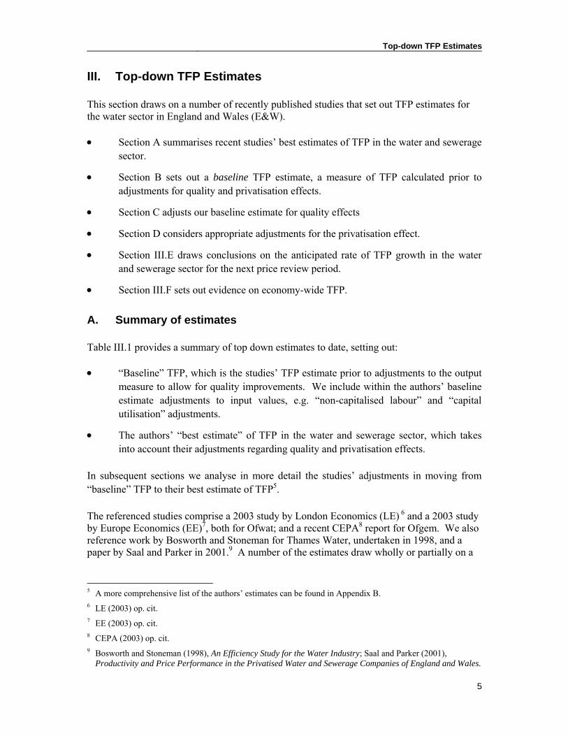
III. Top-down TFP Estimates

This section draws on a number of recently published studies that set out TFP estimates for the water sector in England and Wales (E&W). • Section A summarises recent studies’ best estimates of TFP in the water and sewerage

sector.

• Section B sets out a baseline TFP estimate, a measure of TFP calculated prior to adjustments for quality and privatisation effects.

• Section C adjusts our baseline estimate for quality effects

• Section D considers appropriate adjustments for the privatisation effect.

• Section III.E draws conclusions on the anticipated rate of TFP growth in the water and sewerage sector for the next price review period.

• Section III.F sets out evidence on economy-wide TFP.

A. Summary of estimates

Table III.1 provides a summary of top down estimates to date, setting out: • “Baseline” TFP, which is the studies’ TFP estimate prior to adjustments to the output

measure to allow for quality improvements. We include within the authors’ baseline estimate adjustments to input values, e.g. “non-capitalised labour” and “capital utilisation” adjustments.

• The authors’ “best estimate” of TFP in the water and sewerage sector, which takes into account their adjustments regarding quality and privatisation effects.

In subsequent sections we analyse in more detail the studies’ adjustments in moving from “baseline” TFP to their best estimate of TFP5.

The referenced studies comprise a 2003 study by London Economics (LE) 6 and a 2003 study by Europe Economics (EE)7, both for Ofwat; and a recent CEPA8 report for Ofgem. We also reference work by Bosworth and Stoneman for Thames Water, undertaken in 1998, and a paper by Saal and Parker in 2001.9 A number of the estimates draw wholly or partially on a

5 A more comprehensive list of the authors’ estimates can be found in Appendix B. 6 LE (2003) op. cit. 7 EE (2003) op. cit. 8 CEPA (2003) op. cit. 9 Bosworth and Stoneman (1998), An Efficiency Study for the Water Industry; Saal and Parker (2001),

Productivity and Price Performance in the Privatised Water and Sewerage Companies of England and Wales.


6

NIESR10 sector productivity dataset, so we provide estimates directly from NIESR data for the water, electricity and gas sectors. 11

Table III.1 Summary of TFP Estimates

Author Service Primary dataset

Time period TFP Estimate (% per year)

Baseline: before quality adjustments

etc.

“Best estimate” after adjusting for

quality etc.

Direct estimates (based on water and sewerage data)

LE Water5 ONS/NIESR 1990-2000 0.531 1.21 / 0.72

S&P Water & sewerage June Returns 1990-1995 -0.6 2.11 S&P Water & sewerage June Returns 1995-1999 -0.1 1.01 S&P Water & sewerage June Returns 1990-1999 -0.3 1.61 CEPA Water & sewerage Reg. Accounts 1994/5 - 2001/2 -0.12 2.64, 3

CEPA Water & sewerage Reg. Accounts 1995/6 - 2001/2 0.32 2.64, 3 Indirect estimates (based on comparator sectors) EE Water NIESR 1973-1999 n/a 2.043,6 EE Water NIESR 1989-1999 n/a 1.983,6 EE Sewerage NIESR 1973-1999 n/a 2.033,6 EE Sewerage NIESR 1989-1999 n/a 1.873,6 NIESR Electricity, gas, water NIESR 1970-1999 n/a 3.713 NIESR Electricity, gas, water NIESR 1990-1999 n/a 3.733 NIESR Electricity, gas, water NIESR 1995-1999 n/a 3.553 B&S Water & sewerage ONS 1979-1989/90 n/a 1.2 B&S Water & sewerage ONS 1990-1994 n/a -0.027 Source: NERA derivation from referenced studies. (1) Average annual % change. (2) Linear trend. (3) Compound annual growth rates. (4) Quality adjusted output measure. (5) LE consider this is the best measure for sewerage as well. (6)These data relate to EE (2003a). In their follow-up report in November 2003 (EE (November 2003) “Uncertainties and Measurement Issues”, p28, EE set out a central estimate of 1.9% per annum for water and for sewerage. (7)B&S (1998) Executive summary, p. viii, Table II

As set out in Table III.1, the authors’ best estimates of TFP are relatively wide-ranging, from nearly 4% for NIESR data on electricity, gas and water composite index, to –0.02% p.a. estimated by Bosworth and Stoneman. However, we can also see that the studies’ baseline estimates (for the direct studies using water and sewerage data) fall in a narrower range, of approximately –0.6% to +0.5%.

10 The National Institute of Economic and Social Research: http://www.niesr.ac.uk/ 11 We also look at the recent study by Stone and Webster for Ofwat on economies of scope and scale which

references partial factor productivities (see Section IV.A.1.). See Stone & Webster (2004), An investigation into opex productivity trends and causes in the water industry in England & Wales – 1992-93 to 2002-03, Final Report to Ofwat.


7

The studies’ estimates are differentiated according to the data source used and the authors’ particular approach to constructing the TFP index, particularly the “capitalised labour” adjustment (see Section B). The studies are also differentiated according to whether they rely on direct estimates or comparator sectors; their approach to quality adjustments; and the time period (in particular, whether they include any “privatisation effect”). Our approach to estimating TFP for the E&W water and sewerage sector is to identify the most reasonable baseline TFP figure. We then consider what adjustments are required to this figure, in terms of quality and privatisation effects, to derive our anticipated TFP figure for E&W companies over the next review period. B. Estimating Baseline TFP

The studies divide into those based on direct evidence of TFP growth rate (LE, CEPA and S&P) and those based on comparator sectors (EE, B&S and NIESR data for electricity, gas and water sectors). Regarding direct estimates of the baseline TFP for water and sewerage sector, we note that: • LE’s estimate of TFP for water and sewerage sector is +0.53%12, based on the period

1990-2000 and taking a geometric mean (CAGR).

• CEPA’s baseline TFP estimate, based on companies’ regulatory accounts, is between –0.1% or is 0.3% (also CAGR) depending on the time period.

• S&Ps baseline figure for the period 1990-1999 is -0.3%.

Our reported baseline figures for LE and S&P include their adjustment for “non-capitalised labour”. The authors’ note that a substantial proportion of employment costs in the water industry are attributed to capital projects. Therefore, an index of non-capitalised employment was generated to avoid double-counting of labour inputs and capital costs in the TFP productivity estimates (these labour costs are included in the capital measure of inputs).13 For LE, this adjustment is equivalent to an uplift in their baseline TFP estimate of around 0.4%. The reported baseline LE figure of 0.53% also includes the effect of an adjustment for capital utilisation, although this is relatively small (at -0.03%). Table III.1 also presents data from NIESR’s electricity, gas and water TFP index, which is the basis for a number of the referenced studies. However, the published version of this index does not segregate water and sewerage from electricity and gas. As a result, studies such as that by LE only used some of the information in the dataset along with more disaggregated water sector level data. The results obtained directly from NIESR of around +3.5-3.7% are significantly higher than the baseline estimates derived from other studies. 12 LE report a “baseline” TFP estimate of 0.16% p.a. We also include within our definition of “baseline” any

adjustment for non-capitalised labour, which LE estimate at +0.4%, and a –0.03% adjustment for “capital utilisation”. See LE (2003) op. cit. p.41.

13 See Saal and Parker (2001) op. cit. p73.


8

However, we do not consider these results to be indicative of the scope for TFP improvements in the water sector because of the dominance of energy sector data in the composition of the TFP figure. EE’s estimates are based on a comparator industry approach. EE broke down water and sewerage into industry components and then chose comparator sectors for each component. The TFP figures for these were then aggregated into an overall number using the component shares of operating costs as weights, to produce “water and sewerage comparators” TFP estimates of around +2%. EE’s comparators include sectors such as financial and business services, which are sensitive to changes in economic conditions. EE also include sectors such as mining and extraction, which are experiencing major structural changes. LE also undertook a similar approach but considered the results unreasonable. As a result, we consider that the numbers arrived at by EE are less reliable than those obtained by estimating TFP directly using specific water and sewerage data (e.g. CEPA, LE and S&P). In conclusion, we believe that the studies undertaken using direct evidence from the water and sewerage sector provide a more robust basis for forecasting future anticipated productivity changes in the water sector. Thus, we prefer to place greater emphasis on the baseline estimates of TFP from LE, CEPA and S&P. The three studies report a range of TFP estimates from –0.6% to +0.53%. Taking an approximate mid-point, we adopt a baseline TFP figure of 0% p.a. C. Adjusting Baseline TFP Estimates for Quality

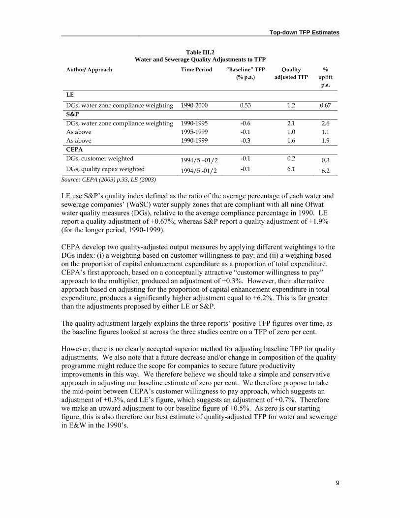
The UK water industry has in recent years been subject to increasingly tighter quality obligations, resulting in large sums of money being spent on compliance. Not taking account of changes in the quality of the outputs will underestimate the true productivity gains in the water and sewerage sector. This is because the cost of quality enhancements will be reflected as an input cost, but there is no corresponding increase in the measure of outputs, because our referenced studies use outputs measured in physical terms. Adjusting for quality involves applying a quality index to the measure of physical outputs, to derive a quality-adjusted output measure. However, there is so far no standard methodology for making quality adjustments to outputs in the water industry and our referenced studies differ substantially in their approach to making adjustments for quality changes. Of the studies presented, LE, S&P and CEPA explicitly set out their quality adjustment. These are presented below. The adjustment for quality varies widely according to the approach taken. CEPA’s quality adjustments range from +0.3% to +6.2%; LE’s adjustment is equal to +0.67%; and S&P report a quality adjustment of +1.9% for the longer period 1990-1999.


9

Table III.2 Water and Sewerage Quality Adjustments to TFP

Author/ Approach Time Period “Baseline” TFP (% p.a.)

Quality adjusted TFP

% uplift

p.a.

LE

DGs, water zone compliance weighting 1990-2000 0.53 1.2 0.67 S&P DGs, water zone compliance weighting 1990-1995 -0.6 2.1 2.6 As above 1995-1999 -0.1 1.0 1.1 As above 1990-1999 -0.3 1.6 1.9 CEPA DGs, customer weighted 1994/5 –01/2 -0.1 0.2 0.3 DGs, quality capex weighted 1994/5 -01/2 -0.1 6.1 6.2

Source: CEPA (2003) p.33, LE (2003) LE use S&P’s quality index defined as the ratio of the average percentage of each water and sewerage companies’ (WaSC) water supply zones that are compliant with all nine Ofwat water quality measures (DGs), relative to the average compliance percentage in 1990. LE report a quality adjustment of +0.67%; whereas S&P report a quality adjustment of +1.9% (for the longer period, 1990-1999). CEPA develop two quality-adjusted output measures by applying different weightings to the DGs index: (i) a weighting based on customer willingness to pay; and (ii) a weighing based on the proportion of capital enhancement expenditure as a proportion of total expenditure. CEPA’s first approach, based on a conceptually attractive “customer willingness to pay” approach to the multiplier, produced an adjustment of +0.3%. However, their alternative approach based on adjusting for the proportion of capital enhancement expenditure in total expenditure, produces a significantly higher adjustment equal to +6.2%. This is far greater than the adjustments proposed by either LE or S&P. The quality adjustment largely explains the three reports’ positive TFP figures over time, as the baseline figures looked at across the three studies centre on a TFP of zero per cent. However, there is no clearly accepted superior method for adjusting baseline TFP for quality adjustments. We also note that a future decrease and/or change in composition of the quality programme might reduce the scope for companies to secure future productivity improvements in this way. We therefore believe we should take a simple and conservative approach in adjusting our baseline estimate of zero per cent. We therefore propose to take the mid-point between CEPA’s customer willingness to pay approach, which suggests an adjustment of +0.3%, and LE’s figure, which suggests an adjustment of +0.7%. Therefore we make an upward adjustment to our baseline figure of +0.5%. As zero is our starting figure, this is also therefore our best estimate of quality-adjusted TFP for water and sewerage in E&W in the 1990’s.


10

D. Adjusting TFP Estimates for Privatisation Effect

The privatisation effect is a term applied to capture the transitory productivity gains that are presumed to have followed the restructuring of the E&W water sector in 1989. We should note that although it is referred to as the “privatisation” effect, in the context of E&W water sector, it effectively captures both the effect of a change of ownership, and the effect of a change to an incentive-based regulatory regime. TFP estimates that are based on direct evidence from the water sector include a privatisation effect to varying degrees, depending on the timescale chosen. Evidence from comparator sectors excludes a privatisation effect, unless the comparators are industries which have also undergone privatisation and regulatory reform; e.g. combined water and energy sectors. Our review of previous studies suggests there is disparate evidence on the importance of the change in ownership and change in regulatory regime in E&W, and on the magnitude of the overall effect embedded within the TFP estimates based directly on water sector data. In their 2000 study, S&P conclude that the efficiency gains which occurred after the privatisation of the water and sewerage industry were “not so much attributable to privatisation per se, but rather to the system of economic regulation that was implemented at privatisation and made more stringent in 1994/1995.” 14 However, in their subsequent 2001 study, S&P conclude that the data does not support the hypothesis that the regulatory review of 1994/1995 increased productivity in the water industry.15 LE find that there is a substantial jump in TFP immediately post-privatisation in 1990. The inclusion of this one-year’s data significantly increases their CAGR-based TFP estimates, although it only has a small effect on their preferred TFP estimates, which are based on trend analysis.16 Regarding the future extent of the privatisation effect, LE comment that they do not expect the privatisation effect to persist over the period 2005-2010.17

EE compare TFP for comparators with observed opex for privatised companies and conclude that the “privatisation effect has been somewhat larger and longer lasting than expected”18. They do not find evidence of a systematic slow-down in productivity improvement after privatisation. On this basis, EE incorporate an upward adjustment to TFP for a “privatisation effect” of +0.5 to +2.5% per annum, to apply over the 2003-2013 time period. EE subsequently revised their estimate of the privatisation effect to +1% to +2%. We do not

14 D. Saal and D. Parker, The impact of privatisation and regulation on the water and sewerage industry in

England and Wales: A Translog Cost Function Model, Managerial and Decision Economics; 21: 253-268, 2000

15 Saal and Parker (2001) op. cit., p88. 16 LE report that their annual average water TFP growth rate of 1.2% per annum for 1990-2000 decreases to

0.31% if 1991 is excluded from the calculation. 17 LE (2003) op. cit., p69. 18 EE (2003) op. cit. p.88


11

consider their estimates, which are derived from real unit operating expenditure changes (RUOE) and assumptions about factor substitution, to be robust.19,20 We also note that in a subsequent update to their report for Ofwat, EE concluded that the extent to which the privatisation effect will continue in the future was “unknowable”. 21 Our preferred estimate of TFP of +0.5% is predominantly based on estimates derived for the period 1990-2000. We consider that any embedded privatisation effect within this estimate will have substantially diminished by the period 2005-2010. Taking account of the uncertainty surrounding this issue, we therefore revise our TFP estimate downwards by a conservative value of 0.1% to 0.4%. This is smaller adjustment than our referenced studies estimates of the privatisation effect, but reflects the fact that there is no clear consensus on the initial size or the subsequent diminution of this effect. It is also consistent with a conservative estimate for the quality effect, as the two adjustments offset each other. E. Summary of TFP Estimates for Water and Sewerage Sector

The referenced studies set out in Table III.1 provide a range of estimates for TFP, ranging from approximately zero, for a study by Bosworth and Stoneman, to nearly +4%, based on NIESR data for the water, electricity and gas sectors. The studies’ results are differentiated according to whether they rely on direct estimates or comparator sectors; their approach to quality adjustments; and the time period observed (in particular, this may or may not include any “privatisation effect”). We believe that direct evidence, drawing on adjusted NIESR data or June Returns, is preferable to evidence based on comparator sectors. In particular, the NIESR estimates based on the water, electricity and gas sectors are significantly higher than the other studies; and we do not consider them to be indicative of the scope for TFP improvements in the water sector because of the dominance of energy sector data. We also have serious reservations about the comparator sectors used by EE in constructing their TFP estimates. Similarly, we note that LE dismissed their comparator based approach to estimating water sector TFP because of the subjectivity involved in selecting comparators, and the sensitivity of estimates to this selection. We therefore conclude that the most robust and appropriate evidence for setting water and sewerage sector TFP is from LE’s recent study for Ofwat; CEPA study for Ofgem; and S&Ps 2001 study. From these studies, we observe that the three studies estimate baseline TFP (after taking into account non-capitalised labour) of +0.53% for LE, +0.1% on average for CEPA, and –0.1% to –0.6% for S&P. We therefore consider that the best estimate of the baseline TFP figure is around 0% for water and sewerage services representing the approximate mid-point of the range from –0.6% to +0.53%.

19 EE (2003) op. cit. p.87. 20 EE (2003b), Uncertainties and Measurement Issues, p.6. 21 EE (2003b), op. cit., p.8.


12

The three studies then make very different adjustments for quality. LE and S&P’s adjustment for quality is based on the proportion of water zones that comply with Ofwat’s DGs, borrowing the approach developed by S&P in their 2001 study. This approach increases the baseline TFP figure by approximately 0.7% for LE and 1.9% for S&P. CEPA uses “quality enhancement weighted” and “customer willingness to pay” weighted quality adjustments. The first approach suggests an adjustment of +0.3%. CEPA’s second approach, which suggests an upward adjustment of 6.2%, is far greater than all other estimates. Our survey suggests that there is as yet no clearly accepted adjustment for quality, and that all the applications to date involve substantial subjectivity. In the absence of a clearly superior approach, and noting that a future decrease and/or change in composition of the quality programme might reduce the scope for companies to secure future productivity improvements, we take a conservative approach and adopt the mid-point of the two lower estimates: CEPA’s “customer willingness to pay” approach which suggest an upward adjustment of 0.3%, and LE’s adjustment for quality of approximately +0.7%. This leads us to an upward adjustment for quality of 0.5%. We conclude that the most reasonable estimate for quality adjusted TFP growth in the water and sewerage sector (prior to an adjustment for the privatisation effect) is +0.5%. Because our preferred estimate of +0.5% is based on evidence from E&W in 1990-2000, it implicitly incorporates any privatisation effect from E&W over this period. We consider that any transitory gains from privatisation will be substantially eroded by the period 2005-2010, more than fifteen years following privatisation. We therefore revise downwards our estimate of the anticipated TFP by a conservative value of 0.1% to +0.4%. F. Estimating Economy-Wide TFP

As set out in Section II.B above, we adopt the standard approach to setting X as espoused in the economic literature.22 This approach requires that the industry specific TFP is offset against the economy wide TFP estimate in setting X, when the price cap is indexed for inflation in economy-wide output prices. Table III.3 we set out our referenced studies’ best estimates of whole economy TFP (where these exist), and also latest estimate from NIESR dataset, which is the basis for all our referenced studies’ economy-wide TFP estimates.23 These estimates are based on the period post-early 1970s oil shock. In common with our referenced studies, we prefer long-run estimates of economy wide TFP because short-run estimates can be influenced by the economic cycle. We also prefer estimate post-1970s oil shock because of possible structural changes in the economy at this time. (Appendix C gives more details on whole economy estimates for different time periods.)

22 See Bernstein and Sappington (1999) Setting the X Factor In Price Cap Regulation Plans, Journal of

Regulatory Economics; 16:5-27. 23 Mary O’Mahony and Willem de Boer (2002), Britain’s relative productivity performance: Updates to 1999,

Final Report to DTI/Treasury/ONS


13

Table III.3 Economy-wide TFP Estimates

Author Time Period Estimate (% per annum)

EE 1974-1999 1.3 CEPA 1979-1999 1.3 NIESR (2002) 1974-1999 1.4

Source: NERA review of referenced studies. As set out, there is a relatively broad consensus regarding economy-wide TFP; EE and CEPA set an economy-wide TFP of +1.3% p.a. and NIESR dataset +1.4% p.a. The differences in the estimates relate to the time period considered, and also the use of geometric and arithmetic averages. In their report, LE estimate a whole economy TFP of 1.55%. However, because it covers a shorter period of time (1979-1989), we do draw on this estimate in adopting our TFP estimate for the period 2005-2010. We assume that economy-wide TFP during AMP4 will be in line with the long run historic estimate of +1.3% p.a. G. Conclusions on “Net TFP”

Under our approach to estimating X, we have to estimate the anticipated TFP growth for the water and sewerage sector relative to the whole economy. On the basis of top-down evidence, we consider that –0.9% p.a. is a reasonable estimate of the expected differential in TPF growth for the period 2005-10 (see Table III.4).

Table III.4 Relative TFP Growth for Water and Sewerage Sector, 2005-10

TFP (% p.a.)

1. Water and sewerage sector TFP growth 0.4 2. Whole-economy TFP growth 1.3 3. Anticipated differential (=1-2) -0.9

Source: NERA analysis.

Top-Down Non-capital and Capital PFP

14

IV. Top-Down Non-capital and Capital PFP

This section sets out the evidence on partial factor productivities for capital and non-capital inputs, typically either opex or labour, drawing on top-down evidence. TFP measures the rate of change of outputs relative to all inputs, whereas partial factor productivity (PFP) is a measure of the rate of change of output relative to a single input. PFPs will differ from TFP to the extent that there are differential growth rates in the use of different inputs. Empirically, we typically observe a higher factor productivity for labour relative to capital in the water sector because the growth of capital inputs is greater (or less negative) than the growth of labour inputs.

PFP measures can be estimated directly, or inferred from TFP estimates on the basis of assumptions about factor substitution and factor shares (see Appendix B).

This section is structured as follows:

• Section A sets out partial factor productivity measures relating to opex and capex.

• Section B draws conclusions on PFP measures consistent with our estimate of TFP of +0.4%.

A. Capital and Non-Capital PFP

1. Non-capital PFP

Non-capital TFP estimates focus on either opex TFP, which includes labour plus materials and other factors of production, as well as estimates for labour TFP, which comprises the largest component of opex. We set out estimates for labour PFP, and opex PFP for our preferred referenced studies (i.e. excluding estimates based on comparators) in Table IV.1. We also present the differential between the studies PFP estimate and associated TFP. This is because the differential between PFP and TFP is indicative of the difference in growth rates between labour and capital, as well as the relative factor shares.24 CEPA is the only one of our referenced studies to estimate PFP for all inputs relating to opex. As set out, CEPA estimate a PFP for opex of +1.4% to +2.0% depending on the time period, which is between 1.1 to 2.1% higher than their estimate of TFP. Thus, this supports the existence of capital substitution in the water and sewerage industry.

24 For example, the differential between capital PFP and TFP can be stated

as: ))()((*)1()()( ,, tttktkt kglgsTFPgPFPg −−=−


15

Both LE and S&P set out PFPs for labour. This demonstrates high values for labour PFP relative to their TFP estimate. This suggests that the greatest scope for factor substitution is away from labour and in favour of materials and capital inputs.

Table IV.1

Non-capital PFP Estimates Author Time Period Service PFP estimate

(% per year) Baseline TFP

estimate (% per year)

Differential (% per year)

=TFP-PFP

Opex PFP CEPA 1994/5-2001/2 w & s 2.0 -0.1 -2.1 1995/6-2001/2 w & s 1.4 0.3 -1.1 Labour PFP LE 1990-2000 w 2.89 0.16 -2.7 S&P 1985-1990 w & s 2.1 -0.2 -2.3 1990-1995 w & s 2.1 -0.6 -2.7 1995-1999 w & s 5.2 -0.1 -5.3 1990-1999 w & s 3.5 -0.3 -3.8

Source: NERA analysis of referenced studies. Notes: w=water; s=sewerage In their recent report to Ofwat, S&W (2004) have estimated opex productivity for water and sewerage in the UK for 1992/3 to 2002/3 time period. They report an average rate of opex productivity growth rate (between 1993 and 2003) of between +1.67 and +2.02 p.a., with an equivalent rate for WoCs of +1.09 to +1.44 per cent per annum.25 This is consistent with PFP for opex estimated by CEPA. However, we do not have a comparable TFP estimates from the S&W study to estimate the extent of factor substitution. 2. Capital factor productivity

Table IV.2 sets out PFP and TFP estimates for LE, CEPA and S&P: • CEPA: CEPA estimates demonstrate that capital PFP estimates for the sewerage and

water sectors combined are lower than TFP, indicating that over the period of analysis capital inputs have increased at a faster rate than non-capital inputs.

• S&P: S&P estimates a similar PFP estimate to CEPA, ranging from 0% to –0.6% depending on the time period, implying similar levels of capital substitution as estimated by CEPA.

• LE: LE’s estimates of capital productivity is much more negative than CEPA/S&P, and implies a greater degree of substitution.

25 Stone & Webster (2004), An investigation into opex productivity trends and causes in the water industry in

England & Wales – 1992-93 to 2002-03, Final Report to Ofwat


16

Table IV.2 Capital PFP Estimates

Author Time Period Service PFP estimate (% per year)

Baseline TFP estimate

(% per year)

Differential (% per year)

=TFP-PFP

CEPA 1994/5-2001/2 w& s -0.51 -0.11 0.4 1995/6-2001/2 w & s 0.11 0.31 0.2 LE 1990-2000 w -4.21 0.16 4.4 S&P 1985-1990 w & s 0.03 -0.23 -0.2 1990-1995 w & s -0.63 -0.63 0.0 1995-1999 w & s -0.43 -0.13 0.3 1990-1999 w & s -0.43 -0.33 0.1 Source: NERA analysis Notes: w=water; s=sewerage

B. Deriving Consistent PFPs

We derive PFP measures for opex and for capital consistent with our overall estimate for TFP of +0.4%. The relationship between PFP and TFP is set out in Appendix B. This demonstrates that the capital PFP will be less than TFP, by the amount equal to the non-capital share of value multiplied by the differential between non-capital and capital growth rates. All of our referenced studies demonstrate that opex (or a labour proxy) PFP has been greater than capital PFP in the water and sewerage sector, suggesting that capital inputs have increased at a greater rate (or have declined at a lower rate) than opex inputs. In setting anticipated capital and non-capital PFP for the period 2005-2010, we also have to consider the diminution of capital substitution. We would expect the water industry to experience a greater rate of factor substitution post-privatisation (when the water companies were freed of public capital expenditure limits), and therefore we would expect the differential growth rates in the future to be lower than historic outturns. To derive consistent PFPs with out TFP estimate, we make the simplifying assumption that capital PFP is approximately 0.4% lower than PFP, drawing on CEPAs lower estimates. This suggests a capital PFP of 0% p.a. (0.4%-0.4%). From this fixed point, we derive a consistent opex PFP using the equations in Appendix B, and a capital share of value for E&W companies of 60%.26 This equates to a consistent opex PFP of +1%. However, we consider that our overall estimate of +0.4% for TFP is more robust than our estimates of 0% and +1% for capital and non-capital (opex) PFPs. This is because there is strong evidence supporting our TFP figure, whereas there is relatively disparate evidence for PFPs. This is related to differences in our referenced studies in measuring capital and non-

26 Ofwat, Financial performance and expenditure of the water companies in England and Wales, 2002-2003

Report


17

capital inputs, and differences in factor shares and differential growth rates for capital and operating inputs.

This has implications for setting unit capex and unit opex efficiency changes (which combine productivity estimates with prospective changes in input prices), which we draw out in Section VII of this report. We do not proceed further with our PFP estimates, because they are insufficiently robust. As a result we provide no PFP estimates for the sector relative to those in the whole economy.

Bottom-up TFP Estimates

18

V. Bottom-up TFP Estimates

In this section we look at bottom-up estimates of capital efficiency. We briefly comment on LE’s recent component based approach and Babtie’s study for Ofwat at PR99 on cost saving technologies. We also compare LE’s bottom-up estimate with their top-down estimate. Their bottom-up estimates are difficult to reconcile with their top-down estimates, and given our concerns about the robustness of LE’s component based approach (concerns also expressed by LE), we conclude the appropriate basis for estimating productivity is to rely solely on the top-down estimates set out in Section III and IV above. A. LE’s Bottom-up Approach

1. Opex

LE’s bottom-up approach to opex is based on the estimated potential future efficiency gains for six unit cost categories (labour, power, materials, Local Authority rates, EA charges and other operating expenditure) using companies’ annual returns data submitted to Ofwat. Projections were based on simple linear trend extrapolations of best-fit lines over two time periods: 1992/3 to 2002/3 and 1998/9 to 2002/3. However, as LE themselves acknowledge, linear extrapolation will not be an accurate representation of future opex efficiencies as it does not take account of future changes in input prices. This is of particular relevance to the energy inputs, which form a substantial proportion of water sector opex and are forecast to increase substantially over the next review period (see Section VI.A.2). 2. Capex

LE’s component-based approach to estimating capex productivity changes splits capex into base service capital maintenance, capital enhancement, supply-demand balance, enhanced levels of service, and quality expenditure. Each category was then further broken down into infrastructure and non-infrastructure. June Returns historical data and Draft Business Plans submissions for PR04 were used to identify weights for each of these categories. LE have drawn on evidence available from the Babtie Report (1998), ERM’s work for Thames Water (1999)27, reviewed “Ofwat New Technologies and Practices Database”, consulted with industry experts and looked at PR94, PR99 and PR04 Cost Base submissions as well as some June Returns data to estimate the potential scope for cost savings by water sector component.

27 ERM (1999), Investigation into the potential for capital efficiency due to new technology in the water

industry, Final Report to Thames Water


19

Drawing on company and reporter comments, LE conclude that 60% of reported capex “efficiencies” are from procurement and management practices, 30% are not efficiency but rather are data issues, and 10% are from standardisation. 28 LE arrive at an estimate for future scope for annual average capex efficiency of +1.1% per annum for water and +1.4% per annum for sewerage. However, LE do not use this approach in setting overall Xcapex. This is because they consider the bottom-up approach is less robust than estimates derived from their top-down analysis, such that they disregard the bottom-up estimates. B. Comparing LE’s Top-down and Bottom-up Estimates

The best practice check-list postulates that bottom-up estimates be used as a test of top-down estimates.

LE’s best estimates of water and sewerage TFP is 0.7%, although they also report a range of values from +0.1% to +1.29% based on a 90% confidence interval. LE’s bottom-up estimates are based on analysis of unit cost trends for opex and a wider set of analysis for capex. We present LE’s point estimates for bottom results, which are derived from two different scenarios. The set of results are set out in Table V.1.

Table V.1 LE's Top-down and Bottom-up Results

Top-down results Bottom-up results

Water Opex +0.7 +2.9 Capex +0.7 +1.1% Sewerage Opex +0.7 +0.9 Capex +0.7 +1.4%

Source: LE (2003), p.118. This table sets out LE’s point estimates for top-down and bottom-up TFP. LE also report a range of 0.1% to 1.3% for top-down TFP estimate based on a 90% confidence interval. They also report a range of values for their bottom-up estimates based on different scenarios.

There are two-offsetting effects that need to be considered in reconciling LE’s top-down and bottom-up opex figures: • LE’s figure for water and sewerage opex productivity does not take into account the

scope for factor substitution. Taking this into account would increase both of these figures, potentially bringing their opex top-down estimates closer in line with their bottom-up estimates.

28 We note that the Babtie estimate of 30% of standard cost changes related to data issues is based on 30% of

companies reporting this as an issue. We do not consider these figures to be robust.


20

• Offsetting this, LE’s top-down opex figure excludes input price effects whereas they are included within the opex bottom-up figures.29 In Section VI.A, we demonstrate that future opex input price growth will be greater than RPI. This means that LE’s top-down opex estimates need to be revised downwards.

These off-setting effects suggest that LE’s opex figures for water are inconsistent (although the opex estimates for sewerage might be closer). For capex, LE’s top-down figures exclude the effect of capital substitution. Taking into account capital substitution, would result in the top-down capex estimates being revised downwards. We note that their bottom-up estimates are already on the upper-boundary of their top-down estimate; a revision for capital substitution would therefore make the two sets of results diverge further. This analysis suggests that LE’s top-down and bottom-up approaches result in quantitatively different TFP and PFP estimates. On the basis of our concerns about bottom-up estimates, we prefer to base our TFP and PFP estimates on top-down studies only. C. Babtie Report on Cost Saving Technologies

In 1998 Babtie were commissioned to update an earlier database and report on technologies and practices that might lead to capital efficiencies in the water industry over AMP3 and to provide an opinion on their potential for the wide scale adoption. As a result, Babtie30 have identified 176 technologies and practices in the four sectors that they looked at: water, sewerage, sludge, and business/general.

Table V.2 summarises Babtie’s findings and shows that their assessment of cost savings in water and sewerage over 2000-2005 is +8% to +16%. However, due to uncertainties in projecting the take-up and effect of new technology, Babtie took a conservative view and their final estimate presented to Ofwat was +5% to +10% over 2000-2005 or a maximum of +2% per annum. At the time, Ofwat applied a compound rate of +1.4% a year on base service and +2.1% a year on quality enhancements. However, the Competition Commission decided that capital maintenance and quality enhancement frontier movement should be set at +1.4%. However, the Babtie report predominantly focused on existing technologies and we would expect (as E&W companies stated) that most of these techniques were already implemented by water companies, and therefore +1.4% may overstate the capital efficiency potential.

29 LE’s bottom-up estimates of TFP are based on the assumption that past trends in input prices will continue.

We do not believe that this is a plausible assumption. In Section VI, we demonstrate that input price changes are expected to increase over the next control period.

30 Babtie Environmental (1998), Report and opinion on the scope for widescale adoption of lower cost new technologies and practices in the water industry, Final Report to Ofwat


21

Table V.2 Summary of Likely Capital Cost Savings 2000-05 as Identified by Babtie

Sector Name of Technology Capital (%) Saving 2000-2005

Water Accuracy of Design Data 1 to 2.5 Chemical Conditioners to combat internal corrosion and

Plumbosolvency 2.5 to 5

Trenchless (no-dig) Techniques 1 to 2.5 Reducing Demand (metering, greywater, leakage) +10 to +20 Sewerage Accuracy of Design Data 1 to 2.5 Sequencing, Batch Reactors (SBRs) 1 to 5 Membrane Technologies 2.5 to 5 Sludge Incineration 3 to 5 Pasteurisation and drying 5 to 10 Land application 10 to 15 Gasification 1 to 3 Business/General

Externalisation of Operations/Services 2.5 to 5

Partnering and procurement methods 5 to 10 Proportion saved 8% to 16% Final estimate (over five years) 5% to 10% Source: Babtie – Table 1, Table 3.5.1, Table 4.9.1, Table 5.10.1, Table 6.9.1 D. Conclusions on Bottom-up Approach to Estimating TFP

Recent experience shows that, to be valid, bottom-up studies must be undertaken at company level, taking account of very specific company circumstances rather than at industry or sector level. The LE results demonstrate that their top-down estimates are very different from their bottom-down estimates. In view of the inconsistency and given that top-down TFP results are based on water and sewerage sector data, we base our conclusions on anticipated TFP exclusively on the consistent set of top-down estimates rather than less robust bottom-up results.

Forecasting Relative Input Price Changes

22

VI. Forecasting Relative Input Price Changes

To derive anticipated changes in unit costs in the water and sewerage sector, i.e. “X”, we need to make an adjustment to our best estimate of productivity growth to take into account relative input price changes. The first part of this section sets out in brief our indicative forecasts for nominal input prices for water companies. These are based on published external forecasts and commentary and on an extrapolation of past trends. We take separate account of opex inputs and capex inputs and derive an indicative input price forecast for each. A more detailed description of the analysis underlying our forecasts is presented in Appendix E. We also need to calibrate our forecasts to be relative to input prices in the whole economy. We discuss this in Section VI.D. A. Opex Input Price Forecasts

The classification of inputs within opex that we adopt for the purpose of forecasting input prices is based on June Returns, Table 21 (water) and Table 22 (sewerage), and broadly follows the classification adopted by LE (2003) in their analysis of component-based unit costs31. This entails the following groups of inputs: • Labour

• Power

• Materials

• Governmental charges (including Local Authority rates, EA charges and other prospective charges such as lane rental charging)

• Other opex (including doubtful debts, bulk water supply imports, exceptional costs and other costs)

In addition, following LE (2003), we have assumed that the costs associated with agencies, hired and contracted services, associated companies, general and support expenditure, customer services, scientific services, other business activities and third party services are comprised of 70% labour and 30% materials costs32. We construct an index tracking real opex input prices based on a weighted average of each input price index in proportion to the relative average expenditures on each input within opex from all companies’ June Return submissions in 2002/3.

31 See London Economics (2003) op. cit. 32 LE (2003) op. cit. pp.71-72.


23

1. Labour prices

Our central forecast for labour prices for England and Wales water companies is based on a UK average earnings forecast drawn from OEF (2004)33. Average earnings forecasts in OEF (2004) are not presented beyond 2008 and so we have taken as our central value for the period 2004/5 to 2009/10 the average of UK average earnings forecasts over 2004 to 2008. Based on the OEF forecast, our forward view for nominal labour prices is 4.4% growth per year. 2. Power prices

A recent OXERA study for Water UK34 estimated that real electricity costs in the UK would rise sharply between 2003/4 and 2005/6 and then remain relatively stable for the following years in K4. Our forecasts for nominal power prices over the K4 period are derived from the OXERA figures for real electricity prices and the average of independent forecasts for RPI drawn from HM Treasury (2004)35. On the basis of OXERA’s “Medium price” forecast, we derive a central forward view of nominal retail electricity price growth of 8.7% per year.

3. Materials prices

Our central forward view of nominal materials price growth is based on a weighted combination of two Producer Price Indices (PPIs), which track the prices of material inputs used by water companies. The two PPIs we use are (i) Electrical Machinery and Equipment; and (ii) Chemicals and Chemical Products and we weight these in the ratio 4:1, which is our understanding of the relative composition of materials and consumables as a component of OPEX in company accounts. To form our view of the trend in real materials prices, we take the period between 1992 and 2003, since these years are both “recovery” years in the economic cycle, and estimate a simple linear regression to the logarithm of the index. This leads to an estimate of the annual rate of growth. The estimated trend for the combined index is –0.02, which equates to a 2% decrease per year in real materials prices.36 We add onto this estimate the average of independent forecasts for RPI over 2004 to 2008 drawn from HM Treasury (2004)37 We acknowledge that our estimate of material prices based on a linear trend might not be a good indicator of future changes in material prices for the water and sewerage sector. In particular, change in energy prices might put upward pressure on future prices. However, in the absence of a cost model for water and sewerage sector materials prices or forecast data,

33 OEF (2004) “Economic Outlook”, April, p.57. 34 OXERA (2004) “Prospects for Retail Electricity Prices”, A Report for Water UK, March 35 HM Treasury (2004) “Forecasts for the UK Economy: A Comparison of Independent Forecasts”, May 36 The adjusted R2 for this regression was 0.91. 37 HM Treasury (2004) “Forecasts for the UK Economy: A Comparison of Independent Forecasts”, May


24

we rely on our linear trend analysis. We believe that this represents a relatively conservative approach.

Our forecast for nominal materials prices is 0.5% growth per year.

4. Governmental charges

The overall level of government charges is likely to be higher in real terms over the forthcoming review period than before. In addition to the introduction of lane rental and BWB charges, there are also significant expected increases in LA rates and possible increases in EA charges. However, the size of the increase in governmental charges is subject to a great deal of uncertainty. Given the uncertainty, government charges should be taken account of separately in price setting as a base opex change or as an NI or RCC. For this reason, for the purpose of forecasting efficiency we assume a conservative increase in governmental charges at the rate of RPI inflation. Therefore, our forward projection for nominal governmental charges is 2.5% growth per year. 5. All other opex inputs prices

In addition to the inputs forecast separately above, water company opex includes a number of other items, which together comprise an average of 8% of water opex and 9% of sewerage opex. These factors include doubtful debts, bulk water supply imports, exceptional costs and other costs. The relative proportions of these factors within opex are highly company specific and hence an industry forecast of the real price associated with this class of inputs would be subject to a high degree of error. We have assumed for the purpose of this study that the real price effect of this class of inputs is zero. Our forward projection for the nominal price of all other inputs is 2.5% growth per year. 6. All opex input prices


25

Table VI.1 presents a summary of our nominal opex input price forecasts for each of the input classes set out above.

Table VI.1 Nominal Opex Input Price Forecasts

Input Weighting1 (%)

Nominal forecast (%/yr)

Labour 46 4.4 Power 7 8.7 Materials 19 0.5 Governmental charges 19 2.5 Other 8 2.5 All Opex 100 3.4 Source: NERA 1 Weights are proportional to the relative average expenditures on each input within opex from all companies’ June Return submissions in 2002/3. We have assumed that the costs associated with agencies, hired and contracted services, associated companies, general and support expenditure, customer services, scientific services, other business activities and third party services are comprised of 70% labour and 30% materials costs.

As set out in

Table VI.1, our forward projection for all opex nominal input prices is 3.4% growth per year.


26

B. Capex Input Price Forecasts

Our forecast for capital expenditure input prices is based on forecasts of construction costs published by DTI and published commentary and forecasts from various sources on construction industry and macroeconomic conditions. We derive our forecast for nominal capex prices as the average of building costs growth forecasts over 2004-2009. On the basis of this evidence, our central forward view of nominal capex prices is 3.4% per year. Our forward projection of nominal capex prices is 3.4% growth per year.

C. Water Sector Input Prices

We combine nominal opex input price projections with nominal capex input price projections to derive a water sector input price projection. The weights of each type of expenditure are 60% for capex and 40% for opex, which we consider are reasonable estimates of the proportions of expenditure in each year over K4. We note that our estimate of expected changes in industry input prices assumes that a number of items are included as base year opex changes or included as a Notified Item or RCC. For example, our estimate of labour costs excludes additional pension costs, which should be included as a base year opex uplift on a company specific basis. We also include a forecast of 2.5%, i.e. no real increase in government charges. This is because the increase in charges is difficult to estimate, and we expect future increases to be addressed as an NI or RCC.

Table VI.2 Water Sector Nominal Input Price Projection

Expenditure type Proportion of total water company expenditure1

(%)

Nominal input price growth (%/yr)

OPEX 40 3.4 CAPITAL 60 3.4 TOTAL 100 3.4 Source: NERA 1 Proportions are estimates for the K4 period.

Our forward projection of water sector nominal input prices is 3.4% growth per year. This excludes anticipated real governmental charges increases relative to RPI.

D. Whole Economy Input Prices

Table VI.3 summarises our estimates of whole economy nominal input price forecasts and presents the weights used to obtain an overall estimate (see also Appendix F).


27

Table VI.3 Nominal Opex Input Price Forecasts

(whole economy)

Input Weight of input within opex (%)

Nominal input price forecast (%/yr)

Labour 56 4.4

Materials and fuels input to the economy

27 2

Capital – (COPI) 4 3.4 Capital- (manufacturing PPI) 13 0.8 All Opex 100 3.2 Source: NERA analysis

Our forward projection of whole-economy nominal input price growth forecast is 3.2% growth per annum.

E. Conclusions on Input Price Effects

Under our approach to setting X, our sector productivity figure is set relative to economy-wide TFP, therefore our sector input price change also has to be relative to whole-economy changes. We conclude that the anticipated sector input price growth rate and economy-wide input price growth rate are 3.4% and 3.2% respectively, giving a relative sector input price effect of 0.2%. We set out the appropriate adjustments to our relative productivity estimate for the water and sewerage sector in Section VII below.

Table VI.4 Relative Input Price Forecast, 2005-2010

Input Price Forecast, 2005-2010 (% p.a.)

1. Water and sewerage input price forecast 3.4 2. Economy-wide input price forecast 3.2 3. W&S sector input price differential (=1-2) 0.2

Source: NERA analysis.

Our analysis shows that expected input price growth in the sewerage and water sector is greater than RPI growth. Our estimate of total water sector input price effects is 3.4%, compared to our estimate of future RPI of 2.5% (i.e. we estimate a price effect relative to economy output prices, RPI, of around 0.9%)

Our figures demonstrate that setting X equal to water and sewerage sector TFP and ignoring input prices would not ex ante provide sufficient revenues to allow companies to finance their activities. Our analysis is consistent with a recent report for Yorkshire Water, which


28

demonstrated that the impact of prospective energy price increases incurred by water companies would not be adequately compensated through the eventual RPI adjustment to allowed revenues (see Appendix H). Finally, our estimate of anticipated economy wide input price effects (3.2%) minus anticipated economy-wide TFP (1.3%) does not equal our forecast of future inflation (of 2.5%), i.e. the equation RPI = Input Priceeconomy – TFPeconomy does not hold because of estimation error. However, it is not clear where the estimation error falls, and whether one or more parameters are mis-estimated. It is also unclear the extent of the error regarding our estimate of water and sewerage sector efficiency. For example, if our economy-wide input price forecast is mis-estimated then quite plausibly our forecast for sector input prices is also subject to mis-estimation. In this case, the mis-estimation error enters twice into our equation for calculating X (see Equation 1, Section II.B) but takes opposite signs and the errors are off-setting.

Setting X: Conclusions

29

VII. Setting X: Conclusions

In this section, we draw together the evidence on productivity and expected input price changes in setting anticipated unit cost changes (or X) over the period 2005-10. A. Estimating X

• The expected change in water and sewerage companies’ unit costs, or X, is equal to the sector wide TFP relative to the whole economy, minus sector wide input prices relative to whole-economy input prices.

• Drawing on LE’s analysis, and analyses by EE, CEPA and S&P, we derive estimates of anticipated TFP improvement and hence efficiency change for the E&W water and sewerage sector for the period 2005-2010.

• The main adjustment we make to the LE approach is that we ensure that productivity and input price effects, both for the sector and the whole-economy, are taken into account in estimating anticipated levels of efficiency improvement.

• First, we review baseline estimates of TFP, defined as estimates prior to adjustments for quality and privatisation effects.

• We consider that top-down estimates based on water and sewerage sector data are the most robust of those available. We do not consider that recent estimates based on comparator sectors are indicative of the scope for efficiency improvements in the water industry. We also consider that estimates based on the bottom-up studies we have reviewed are not robust.

• We find that for the set of top-down TFP estimates based on direct water and sewerage data, the change in TFP over the period 1990-2000 in E&W falls in the range of –0.6% to +0.5%. We adopt the mid-point value of 0% as the most appropriate estimate of “baseline” TFP growth for the water and sewerage sector in E&W.

• We then consider quality adjustments. Our referenced studies have taken a number of different approaches to adjusting for quality, and their estimates are also relatively disparate. In the absence of a clearly accepted methodology for quality adjustments, and noting that a change in the future size and composition of the quality programme might reduce companies’ ability to repeat past productivity improvements, we take an average of two lowest estimates: CEPA’s “willingness to pay” approach and LE’s “water zone compliance” quality adjustment. This suggests an upward adjustment to the TFP figure of 0.5% for quality.

• We also consider the privatisation effect. There is no clear consensus on the size of the privatisation effect or on its diminution. We note that our baseline estimate of 0% includes embedded effects for transitory productivity improvements post-privatisation which we consider will have substantially reduced by 2005-10. We therefore adjust


30

our TFP estimate downwards by 0.1%, which represents a conservative adjustment in the context of estimates set out in our referenced studies.

• Overall, our best estimate of the anticipated TFP in the water and sewerage sector over the next review period is +0.4%per year.

• Consistent with the literature on setting prices in a RPI-X regime, we then net off the total economy-wide TFP figure of +1.3%. We therefore calculate a “net” TFP improvement figure for the water and sewerage sector in E&W of -0.9% per year – sector productivity growth is exceeded by average economy productivity growth.

• We then consider the impact of input prices on anticipated efficiency changes. In deriving anticipated efficiency assumptions, we have to consider the expected level of input price changes for the water sector relative to whole-economy input price changes. Our central forecast of the water sector input price change is +3.4% based on forecasts for the main factors of productions, labour, materials, energy and capital. Our corresponding estimate of the economy-wide input price change is +3.2%. This indicates an input price differential of 0.2% p.a.

Taking together our net TFP estimate with relative input price effects, our best estimate of X is equal to -1.1% (

• Table VII.1), i.e. we anticipate unit costs in the water and sewerage sector, relative to

those in the economy, will increase by 1.1% over the period 2005-10.

• We note that there is uncertainty regarding the value of the constituent elements of our efficiency estimate, both for productivity measures and input price forecasts. In estimating the constituent elements of our efficiency estimate, we believe that we have taken a consistent approach. For example, our quality adjustment is based on a relatively conservative interpretation of the available data; however, our adjustment for the diminution of the privatisation is also based on a conservative approach (and these effects off-set each other). Therefore, we believe our final unit cost estimate of 1.1% is based on a consistent set of parameters.


31

Table VII.1 Derivation of X (% p.a.)

Step % per year

a. “Baseline” TFP estimate 0% b. Quality adjustment +0.5% c. Privatisation effect adjustment -0.1% d. Quality adjusted TFP (=a+b+c) +0.4% e. Economy-wide TFP estimate +1.3% f. Relative TFP estimate (=d-e) -0.9% g. Water sector input prices adjustment +3.4% h. Economy-wide input prices adjustment +3.2% i. “X” (=f-(g-h)) -1.1% j. Anticipated change in real unit costs (=-i) +1.1% Source: NERA analysis and review of referenced studies. B. Setting Xcapex and Xopex

• We do not estimate separate Xcapex and Xopex forecasts.

• We consider that our overall estimate of overall efficiency savings (“X”) is more robust than separate estimates. This is because there is relatively disparate evidence on the capital and non-capital PFPs, which makes estimating unit changes in separate cost lines, Xopex and Xcapex, more difficult than estimating the change in total unit costs. Also, consistent Xopex and Xcapex targets will be company specific because of differences in scope for factor substitution and different factor shares.

• In the context for this study the key issue is that the overall package of ex ante “efficiency adjustments” to inputs to the financial modelling produces a revenue forecast which allows companies to finance their activities. The overall revenue effects of applying a single X to both opex and capex expenditure lines is equivalent to applying individual (consistently derived) Xopex and Xcapex. Thus, the two approaches are “revenue neutral”.

• Our estimate of X (an increase of +1.1% each year) includes all anticipated types of efficiency gain and is calibrated to be applied to all opex and capex lines. For


32

consistency all opex and capex expenditure lines in companies’ business plans to which the adjustment is applied should be gross of all anticipated efficiencies.

• Ofwat should also make specific allowances for anticipated changes in costs excluded from our input price forecasts. Our estimate of future labour costs excludes pension costs, which we believe are more appropriately treated as a base opex uplift. In addition, our government charges input price change is set equal to RPI at 2.5%, in anticipation that these charges (LA rates; EA charges etc.) are addressed through notified items (NI) and relevant change of circumstance (RCC) clauses in companies’ licenses.

• Our productivity estimate of 0.4% relates to the anticipated change in total productivity, i.e. it comprises both the frontier movement and average industry “catch-up”. In estimating the scope for the movement of the frontier, and the average rate of industry catch-up to the frontier, Ofwat should reconcile the sum of these figures to our estimate of the industry productivity figure of 0.4% (and not the anticipated unit cost increase of 1.1%).

Appendix A

33

Appendix A. Some Proposals for an Agreed Methodology for setting EffIciency

• Water company cost trends

- uninformative unless allow for prices

- better to review productivity trends

- forecasts reflect diminishing scope for productivity

• Top down TFP based estimates

- reflect difference to economy as a whole

- base on relevant comparators

- TFP split into capex and opex productivity – used consistently

- add price effects – not assume as zero

• Bottom up productivity and price forecasts

- reflect difference to economy

- base on relevant comparators

- estimate labour and materials productivity and prices

- and combine

- provides a key test of top down estimates

• International comparisons

- use as benchmark

- but significant health warning

- different measures of output and operating environment

- rates of change may have some relevance

- productivity levels unlikely to be comparable

Appendix B

34

Appendix B. Water sector TFP Estimates

Table B.1 Current Water Sector TFP Estimates (% per annum) Sector Author Adjustments

1974

19

75

1976

19

77

1978

19

79

1980

19

81

1982

19

83

1984

19

85

1986

19

87

1988

19

89

1990

19

91

1992

19

93

1994

19

95

1996

19

97

1998

19

99

2000

20

01

2002

Water & sewerage

S&P 2.2

2.0

0.8

Appendix B

35

Sector Author Adjustments

1974

19

75

1976

19

77

1978

19

79

1980

19

81

1982

19

83

1984

19

85

1986

19

87

1988

19

89

1990

19

91

1992

19

93

1994

19

95

1996

19

97

1998

19

99

2000

20

01

2002

1.4

CEPA -0.3

Volume -0.3

Quality 7.7

Quality & volume 7.7

Customer value weighted quality

0.1

Water

CEPA -1.0

Volume -1.0

Quality 10.2

Quality and volume

10.2


-0.5

LE

0.16

Quality 0.83

Labour input adjustment

1.23

Appendix B

36


1974

19

75

1976

19

77

1978

19

79

1980

19

81

1982

19

83

1984

19

85

1986

19

87

1988

19

89

1990

19

91

1992

19

93

1994

19

95

1996

19

97

1998

19

99

2000

20

01

2002

Capacity utilisation

1.20

Sewerage CEPA

0.3

Volume 0.3

Quality 1.5

Quality and volume

1.5


0.4

LE

4.32

Capacity utilisation

3.76

Electricity, gas, water

NIESR 2.43

3.45

3.42

LE

1.42

Labour input correction

1.57

CEPA

2.8

Appendix B

37


1974

19

75

1976

19

77

1978

19

79

1980

19

81

1982

19

83

1984

19

85

1986

19

87

1988

19

89

1990

19

91

1992

19

93

1994

19

95

1996

19

97

1998

19

99

2000

20

01

2002

Volume 2.0

3.4

Volume 3.2

Source: (1) PR04 Scope for Efficiency Studies, Final Report to OFWAT by London Economics, Black & Veatch, and Professor Shutler (2003) (2) Scope for Efficiency Improvement in the Water and Sewerage Industries, Final Report to OFWAT by Europe Economics (2003) (3) Productivity Improvements in Distribution Network Operators, Final Report to OFGEM by Cambridge Economic Policy Associates (2003)

Appendix C

38

Appendix C. Economy-Wide TFP Estimates

Table C.1 sets out economy-wide estimates for our referenced studies, and for different time periods.

Table C.1 Whole Economy TFP Estimates (% per annum)

Author

1974

19

75

1976

19

77

1978

19

79

1980

19

81

1982

19

83

1984

19

85

1986

19

87

1988

19

89

1990

19

91

1992

19

93

1994

19

95

1996

19

97

1998

19

99

2000

20

01

2002

CEPA

1.36

NIESR (latest)

1.4

EE

1.31

CEPA

1.27

NIESR

1.81

LE

1.55

Appendix C

39

Author

1974

19

75

1976

19

77

1978

19

79

1980

19

81

1982

19

83

1984

19

85

1986

19

87

1988

19

89

1990

19

91

1992

19

93

1994

19

95

1996

19

97

1998

19

99

2000

20

01

2002

B&S

0.92

NIESR

1.02

O’Mahoney

1.14

O’Mahoney

1.30

NIESR

1.29

EE

1.14

B&S

1.05

CEPA

1.28

NIESR

0.85

LE

≈1.0

CEPA

0.67

Appendix C

40

Author

1974

19

75

1976

19

77

1978

19

79

1980

19

81

1982

19

83

1984

19

85

1986

19

87

1988

19

89

1990

19

91

1992

19

93

1994

19

95

1996

19

97

1998

19

99

2000

20

01

2002

O’Mahoney

0.90

Sources: LE (2003); EE (2003); O’Mahoney (2002); Bosworth and Stoneman (1998); CEPA (2003).

Appendix D

41

Appendix D. Deriving Capital Efficiency From TFP

Starting with a simple production function (equation 1), where output (Y) at time (t) is a function of non-capital (simplified to labour) (L) and capital (K) inputs at time (t), augmented by TFP at time (t): (1) ),( tttt LKfTFPY = Using standard growth accounting methodology and employing the use of logs, the change in log of output at time (t) can be defined as per equation (2), where tKs , and tLs , are shares of capital and non-capital inputs in total output at time (t) and 1,, =+ tLtK ss . (2) tttLttKt TFPglgskgsyg )()()()( ,, ++= This simply states that the growth in output is equal to the growth in factors of production multiplied by their factor shares, plus TFP growth, where: • Capital inputs consist of the market value of capital employed multiplied by the cost of

providing this capital, plus capital consumption.

• Non-capital inputs are set equal to operating expenditure.

• Shares are set equal to the total input share as a percentage of total costs.

Re-arranging (2), we can derive the relationship between partial factor productivities (capital and non-capital) and total factor productivity. For example, capital productivity can be calculated as: (3) ))()((*)1()()()()( ,, tttktttkt kglgsTFPgkgygPFPg −−+=−= This states that capital factor productivity will differ from TFP, where the difference is calculated as the product of one minus the capital share of total costs multiplied by the difference in the growth rate of the two factor inputs. We can set out the relationship for non-capital factor productivity to TFP in a similar way. The implication of (3) is that if capital inputs grow at a faster rate than non-capital inputs (i.e. there is capital substitution) then capital factor productivity will be less than TFP.

Appendix E

42

Appendix E. Estimating Water and Sewerage Sector Input Prices

This appendix sets out input price forecasts for the water and sewerage sector disaggregated into labour, power, materials, governmental charges and capital. E.1. Labour Prices

The most useful indices available to track labour prices for England and Wales water companies are listed in Table E.1 below.

Table E.1 Labour Price Indices

Index Source

Average earnings (UK) New Earnings Survey, published in ONS “Regional Trends”, various years.

Average Earnings Index (UK) ONS, www.statistics.gov.uk: series LNMM Electricity, Gas and Water industry earnings (UK)1 ONS, www.statistics.gov.uk: series JVUN Electrical labour cost index (UK) BEAMA2 Mechanical labour cost index (UK) BEAMA2

Construction industry labour costs (UK) BCIS “Indices and Forecasts”, various issues 1 The first full year of this series is 2000. 2 Data were purchased directly from BEAMA.

Figure E.1 presents real earnings growth as measured by each of the indices in Table E.1.

Appendix E

43

Figure E.1 Real Earnings Growth (various indices)

(per cent per year)

-4.0%

-2.0%

0.0%

2.0%

4.0%

6.0%

8.0%

1987

Q1

1988

Q1

1989

Q1

1990

Q1

1991

Q1

1992

Q1

1993

Q1

1994

Q1

1995

Q1

1996

Q1

1997

Q1

1998

Q1

1999

Q1

2000

Q1

2001

Q1

2002

Q1

2003

Q1

2004

Q1

NES - Real Earnings (UK)ONS - Real Average Earnings (UK)BCIS - Real Construction Earnings (UK)ONS - Real Electricity, Gas and Water Earnings (UK)BEAMA (Electrical)BEAMA (Mech Eng)

Construction industry earnings have risen dramatically and whole economy earnings have exhibited modest growth. From the limited time period available on electricity, gas and water earnings growth it is difficult to gauge both the volatility of earnings in this sector, or how they are likely to grow in relation to whole economy earnings.

Appendix E

44

Recently published forecasts are available for UK average earnings from OEF (2004)38. In addition, BCIS publish medium-term forecasts for construction industry labour costs on an annual basis. The most recent medium term forecasts available from BCIS were published in August 2003.

Our central forecast for nominal labour prices for England and Wales water companies is based on OEF (2004)39. Average earnings are likely to track water company labour costs with a degree of error due to the

fact that labour cost trends vary by sector and by region. The forecast is presented in

Table E.2.

Table E.2 Central Forecasts for UK Average Earnings Growth

Year UK Average Earnings1

(%/yr)

2004 5.1

2005 4.5 2006 4.2 2007 4.1 2008 4.2

1 Source: OEF (2004)“Economic Outlook”, April, p.57. Forecasts are for years beginning Quarter 1. Average earnings forecasts in OEF (2004) are not presented beyond 2008 and so we have taken as our central value for the 2004/5 to 2009/10 period the average of UK average earnings forecasts over 2004 to 2008. Our central projection for nominal labour prices is 4.4% growth per year. E.2. Power Prices

Real industrial power prices have been falling throughout the past decade.

38 OEF (2004) “Economic Outlook”, April, p.57. 39 OEF (2004) “Economic Outlook”, April, p.57.

Appendix E

45

Figure E.2 shows that real electricity prices paid by industry fell by over 40% between 1990 and 2003. However, the prospects for the forthcoming decade are quite dramatically different according to a recent OXERA study for Water UK40. This study estimated that real electricity costs in the UK would rise by approximately 15% in 2005/6 in comparison with 2004/5, rise by a further 3% the following year and then remain stable for the following three years. The primary explanation given for the sharp increase estimated for 2005/6 is the introduction of the EU Emissions Trading Scheme (ETS), which is predicted to increase the costs of generation from 2005/6.

Figure E.2 Real Industrial Electricity Price Index (1990=100)1

40 OXERA (2004) “Prospects for Retail Electricity Prices”, A Report for Water UK, March 2004

Appendix E

46

0

20

40

60

80

100

120

1990

1991

1992

1993

1994

1995

1996

1997

1998

1999

2000

2001

2002

2003

Source: DTI (2004) “Quarterly Energy Prices”, April. 1 Original (nominal) index has been deflated by RPI. Index includes Climate Change Levy

The full set of retail price forecasts produced by OXERA, including “high” and “low” scenario forecasts, are presented in Table E.3 below.

Table E.3 Retail Price Scenarios for UK Electricity Supplies

Year Estimated starting level

Low price Medium price High price

2003/04 100 - - - 2004/05 111 - - - 2005/06 - 122 128 131 2006/07 - 124 132 139 2007/08 - 122 132 140 2008/09 - 124 134 145 2009/10 - 122 132 147

Source: OXERA (2004), “Prospects for Retail Electricity Prices”, A Report for Water UK, March 2004, p.26 The estimates presented in Table E.3 are focussed on average UK electricity prices and do not take account of regional differences in future electricity prices. Whilst changes in the wholesale cost of electricity, which comprises approximately 75% of total electricity costs, are likely to be similar across England and Wales, transmission and distribution price movements may vary significantly across regions. Electricity distribution costs for the 2005-2010 period are subject to the Distribution Price Control Review conducted by Ofgem. The best current estimates for future distribution costs over the 2005 to 2010 period are given by Distribution Network Operators’ (DNOs’) own forecasts, presented in

Table E.4 below.

Appendix E

47

Table E.4 DNO Forecasts for 2005-10 Distribution Costs

(percentage change 2005-10 over 2000-05)

Company Operating costs1 Net capital expenditure Price control review2

CE – NEDL -1% 5% -14% CE – YEDL -9% 14% -11% CN – East Midlands 0% 71% 3% CN – Midlands 1% 33% 5% EDF – EPN 30% 71% 6% EDF – LPN 20% 95% 16% EDF – SPN 24% 47% 37% SP Distribution -4% 23% 4% SP Manweb -3% 41% 11% SSE – Hydro 3% 21% 7% SSE – Southern 9% 23% 7% United Utilities 3% 23% 9% WPD – S. Wales 3% -5% 8% WPD – S. West 22% 17% 10%

Source: Ofgem (2004) “Distribution Price Control Review Workshop”, 20 April, Presentation by David Gray. 1 Includes NGC exit charges, cost of sales and depreciation. 2 Figures as calculated by companies. Since prices vary significantly across regions, the real power price growth that companies experience may differ considerably from the industry-wide forecasts in Table E.3. Our forecasts for England and Wales power costs are derived from Table E.3. The forecast changes in the table are not readily applicable in adjustments to unit cost forecasts, where we require forecast annual growth rates. For the purpose of exposition of unit cost trends, we convert these forecasts into annual growth rates. A simple division of the total forecast change in level by six would understate the impact of the forecast increases on companies because the increases are front-weighted. We therefore take logs of the medium, high and low price forecasts, subtract from each the initial value, ln(100), and regress each series on a time trend from 0 to 6 with no constant. This procedure results in the best linear approximation of the annual growth rates for 2004/5 2009/10 in each scenario, taking account of the front-loading of the price increases. On the basis of the procedure described above, our central forecast for the growth rate of real electricity prices in 2005/6 – 2009/10 relative to the base year (2003/4) is 6.2% per year. This is based on the “medium price” scenario forecasts in Table E.3. We add onto these estimates the average of independent forecasts for RPI over 2004 to 2008 drawn from HM Treasury (2004)41.

Our central projection for nominal power price growth is 8.7% per year.

41 HM Treasury (2004) “Forecasts for the UK Economy: A Comparison of Independent Forecasts”, May

Appendix E

48

E.3. Materials Prices

Indices tracking the prices of inputs used by UK firms are published by Office of National Statistics (ONS). These Producer Price Indices (PPIs) are suitable for tracking the prices of materials and fuels used by most industry groups. There exists a PPI for water industry inputs for the UK (ONS, series PQNB), which should be the index we are interested in, however unfortunately this index is not suitable since it is based on OPEX allowances within price limits and is thus not appropriate as a guide to the actual prices of materials paid for by water companies. ONS also publish output PPIs, which track the prices of outputs produced by industry group. We construct an index to track the prices of materials used by water companies using a weighted average of ONS output PPIs for the most relevant sectors. It is our understanding that the “materials and consumables” class of OPEX contains mostly spare parts for machinery and equipment and chemicals.

Table E.5 shows the indices we adopt for our analysis.

Table E.5 Materials Price Indices

Description Source Time period

Producer Price Index (Gross Sector Output) Chemicals and Chemical Products

ONS, www.statistics.gov.uk: series POKN

1991 – 2003

Producer Price Index (Gross Sector Output) Electrical Machinery and Apparatus

ONS, www.statistics.gov.uk: series POLN

1991 - 2003

Figure E.3 below charts these indices from 1991 to date.

Appendix E

49

Figure E.3 Real Materials Price Indices

60

70

80

90

100

110

120

1991

1992

1993

1994

1995

1996

1997

1998

1999

2000

2001

2002

2003

Chemical & chemical products Electrical machinery & apparatus n.e.c

1 Original indices have been converted to real prices using RPI and rebased to 1991 =100.

The two series presented in Figure E.3 appear to follow a similar downward trend, however chemicals prices appear to display greater volatility.

Figure E.4 presents a combined index of real materials prices constructed from a weighted combination of electrical machinery and apparatus prices and chemicals and chemicals products prices. The combination is derived using the ratio of 80:20 in favour of the electrical machinery and apparatus index, which we understand is approximately the ratio of expenditures of the two classes of materials and consumables within water company opex.

Appendix E

50

Figure E.4 Real Materials Prices (Combined Electricals and Chemicals Index, 1991=100)

60

70

80

90

100

110

120

1991

1992

1993

1994

1995

1996

1997

1998

1999

2000

2001

2002

2003

To form our view of the trend in real materials prices, we take the period between 1992 and 2003, since these years are both “recovery” years in the economic cycle, and estimate a simple linear regression to the logarithm of the index. This leads to an estimate of the annual rate of growth. The estimated trend for the combined index is –0.02, which equates to a 2% decrease per year in real materials prices.42 We add onto this estimate the average of independent forecasts for RPI over 2004 to 2008 drawn from HM Treasury (2004)43.

We acknowledge that our estimate of material prices based on a linear trend might not be a good indicator of future changes in material prices for the water and sewerage sector. In particular,

42 The adjusted R2 for this regression was 0.91. 43 HM Treasury (2004) “Forecasts for the UK Economy: A Comparison of Independent Forecasts”, May

Appendix E

51

change in energy prices might put upward pressure on future prices. However, in the absence of a cost model for water and sewerage sector materials prices or forecast data, we rely on our linear trend analysis. We believe that this represents a conservative approach.

Our central projection of nominal materials prices growth is therefore 0.5% per year. E.4. Governmental Charges

The governmental charges class of inputs presently includes local authority rates and EA charges, factors that are longstanding components of opex. Together, in 2002/3, these factors comprised an average of 18% of water service opex and 12% of sewerage service opex. Examining past trends in the level of these charges is likely to be misleading in respect of future governmental charges because of the following factors: • Local Authority (LA) rates are set to change from April 2005

• Environment Agency (EA) charges are likely to increase

• Lane rental charging is likely to be introduced

LA rates The Valuation Office Agency (VOA) is working on a new system for charging non-domestic rates for water supply systems to replace the current system of prescribed rates. The new rates will be in place from April 2005. Final decisions on the actual costs to companies will be made available very late in the price setting process. However, Ofwat will take into account the latest information available from the VOA in its final determinations and so the increases are likely to be passed through to prices.

Our understanding at the time of writing is that if companies’ final rates are not sufficiently well known in time for Final Determinations then Ofwat will consider treating LA rates as Notified Item.

EA charges In January 2004, the EA launched a consultation paper, which considered both the issue of funding compensation costs and alternative ways of structuring abstraction charges in light of the Water Act 2003 and EU directive obligations. The Environment Agency estimates that the total compensation bill will amount to £745m, of which £436m is the estimated compensation required by water companies for curtailing water abstraction volumes and the remaining £309m is the estimated cost of compensation for the curtailment of non-water company abstraction

Appendix E

52

licenses44. By contrast, current abstraction charges merely cover the Agency’s annual costs of £108m45. At the time of writing there is a great deal of uncertainty concerning future abstraction charges. Ofwat have not committed to allowing a Notified Item in respect of EA charges but they have stated that they are considering one.46 Lane rental charging Our understanding is that it is highly likely that water companies will be faced with the introduction of lane rental charges for carrying out street works at some point during K4. In March 2002, Stone & Webster Consultants undertook a study for Yorkshire Water on Lane Rental Charging and its implications for Yorkshire Water Services47. For 2000-01, Stone and Webster calculated that the potential total lane rental cost to Yorkshire Water (given their 2000-01 streetworks undertaken) would be about £36m or about 14.5% of their 2000-01 opex. A Draft Regulatory Impact Assessment document, produced by DTLR, estimated the cost of compliance to be between £109m and £334m. However, this was for all utility companies and so implies a substantially lower estimate of the impact on water company opex. Ofwat have stated that additional costs incurred as a result of lane rental charges will be passed through to customers by allowing them to be treated as a Notified Item.48 All governmental charges At the time of writing, the overall size of the increase in governmental charges is subject to a great amount of uncertainty. For this reason, we assume for the purpose of forecasting efficiency that governmental charges increase at the rate of RPI inflation. Our forward projection for nominal governmental charges is 2.5% growth per year. E.5. CAPEX Prices

Construction output prices at a national level are tracked by the Construction Output Price Index (COPI). The index may not closely track the construction prices actually faced by water companies since it is derived from output prices of all construction projects, some of which are very different from water sector capital projects, such as housing developments, commercial 44 Environment Agency (2004), “Review of the water company abstraction charges scheme: Consultation

document”, January, p.14 45 The Ends Report (2004), “Agency warns of steep rise in abstraction charges”, January, Issue No. 348. 46 Ofwat (2004), “MD190: Further guidance to companies for final business plans”, March, p.10 47 Stone & Webster Consultants (2002), “Lane Rental Charging: A Way Forward”, A Revised Final Report for

Yorkshire Water Services, March 48 Ofwat (2003) “Setting water and sewerage price limits for 2005-10: Framework and approach”, March

Appendix E

53

building and road building. Nonetheless we focus on COPI as the measure of capex price inflation for England and Wales water companies since this index is used by Ofwat and by water companies to track capex prices.

Figure E.5 below presents year on year growth rates of COPI and RPI.

Figure E.5 COPI and RPIX Annual Inflation

(per cent per year)

-10.0%-5.0%0.0%5.0%

10.0%15.0%20.0%25.0%30.0%

1976

-1

1978

-1

1980

-1

1982

-1

1984

-1

1986

-1

1988

-1

1990

-1

1992

-1

1994

-1

1996

-1

1998

-1

2000

-1

2002

-1

2004

-1

COPI RPIX

COPI Source: DTI, All New Construction Output Price Index. Note the final two quarterly data points are provisional RPIX Source: ONS; RPIX series code = CDKQ

Appendix E

54

Figure E.6 presents the growth rate of COPI in real terms, i.e. after deducting changes in RPI.

Figure E.6 COPI Inflation Relative to RPI

(per cent per year)

Appendix E

55

-20.0%

-15.0%

-10.0%

-5.0%

0.0%

5.0%

10.0%

15.0%

1976

-1

1978

-1

1980

-1

1982

-1

1984

-1

1986

-1

1988

-1

1990

-1

1992

-1

1994

-1

1996

-1

1998

-1

2000

-1

2002

-1

2004

-1

COPI source: DTI, All New Construction Output Price Index. Note the final two quarterly data points are provisional RPIX source: ONS; series code = CDKQ

It is clear from the figures that COPI follows a cyclical path but that the volatility of real COPI has been significantly lower in recent years. This behaviour is consistent with the generally greater degree of macroeconomic stability experienced in the UK. Since 1997, the difference between COPI and RPIX inflation rates has ranged between –3.6% and +2.3%. There are no publicly available published external forecasts for COPI and it is beyond the scope of this report to produce a full forecast for COPI. We have made use of published expert commentary and forecasts for related indices to form a forward view. The sources we have considered include: • BCIS “Indices and Forecasts”, April 2004

• Hewes & Associates “Construction Outlook”, April 2004

• Experian Business Strategies “Construction Forecasting and Research”, January 2004

• DTI “Quarterly Building Price and Cost Indices”, March 2004

BCIS (2004) forecasts 3.0% growth for 2004 Q1 to 2005 Q1 and 3.9% growth for 2005 Q1 to 2006 Q1. The main drivers for this growth forecast are expected wage settlements above the rate of inflation and a projected growth in demand particularly from the public sector. Neither Hewes & Associates (2004) nor Experian Business Strategies (2004) forecasts construction prices. However, output forecasts in each publication are broadly similar to each other and in line with those of BCIS (2004). In each case, public sector housing and non-housing and infrastructure outputs are forecast to show strong growth between 2004 and 2006 and this drives a modest total construction demand growth over the period.

Appendix E

56

For long term forecasts of construction trends, the most useful information is found in DTI (2004). This publication contains a forecast cost index, which is presented to 2011. This index is a projection of how the DTI’s combined building non-housing costs index is expected to move over the next eight years. It is based on anticipated trends in labour and materials costs and on current and projected inflation policy. Economic theory suggests that in the long run, construction prices should move with costs and so a forecast of building costs is a useful starting point from which to forecast construction prices. Previous NERA studies have confirmed that the primary variables to affect the long run trend level of construction output prices are the resource costs (materials and labour) in the construction industry. In addition, we found that construction output prices deviate around their long run trends according to shorter term market conditions, i.e. demand for new construction (relative to construction capacity), which reflects the wider macro-economic environment. Our forward view of the likely annual growth in real construction output prices is built up in Table E.6 below.

Table E.6 Forward View of Real Construction Price Growth

Building Costs1 RPI2 Real GDP2 Real Construction Prices3

2005 3.8% 2.4% 2.7% 1.4% 2006 3.6% 2.5% 2.4% 1.1% 2007 3.5% 2.6% 2.4% 0.9% 2008 3.4% 2.7% 2.5% 0.7% 2009 3.3% 2.5% 2.3% 0.8% 2010 3.2% 2.5% 2.3% 0.7%

1 Source: DTI”Quarterly Building Price and Cost Indices”, March 2004,p.49, FORVOP index. 2 Source: 2005-2008 forecasts from HM Treasury “Forecasts for the UK Economy: A Comparison of Independent Forecasts”, May 2004; 2009-2010 forecasts from Consensus Economics Inc. “Consensus Forecasts Global Outlook 2003-2013”, Oct 2003. 3 Source: NERA In periods of high growth or recession construction prices tend to depart significantly from resource costs. However, the consensus of analyst forecasts reviewed by HM Treasury and by Consensus Economics Inc. for GDP suggest that economic growth over the medium term is likely to be at around trend level. We therefore base our forward view for real construction prices on the assumption that market conditions in the construction sector will remain stable over the medium term. Our forward view of real construction price growth is built up by subtracting forecast RPI growth from DTI forecasts for nominal building cost growth. We take the average of this series over 2005 to 2010 for our central forecast. On this basis, our central forecast for capex price growth is 0.9% per year in real terms, or 3.4% in nominal terms.

Appendix F

57

Appendix F. Deriving Economy-Wide Input Price Forecasts

We construct an economy wide forecast as a weighted average of the main factors of production (labour, materials and capital), where the weights are determined by the share of value for each factor relative to gross output. We obtained labour and capital share of total output by using National Accounts (The Blue Book) published by the ONS. These are 56% and 17% respectively. We then estimated other inputs (materials and fuels) as a residual proportion of gross domestic product. Table F.1 provides a list of ONS indices that we employed.

Table F.1 ONS Indices Used to Obtain Weights in Opex Price Forecast

Factor input Index

Labour Total compensation of employees (HAEA) Capital Gross capital formation (NQFM) Total output Gross domestic product (YBHA) Other factors of production Estimated as a residual fraction of GDP

Section E.1 Appendix E set out how we derived our nominal labour input price forecast of +4.4% per annum. For materials inputs into the economy we used manufacturing producer input prices forecast published by Oxford Economic Forecasting, which produces an average forecast over the period of approximately 2% p.a. (see Table F.2).

Table F.2 OEF Manufacturing Producer Input Prices Forecast

(Nominal, % Change per Year) Year Producer input prices

2004 1.9 2005 3.2 2006 1.5 2007 0.8 2008 2.4 Annual average 1.96 Source: Oxford Economic Forecasting, Spring Economic Outlook, Volume 28, No.3 We used a combined forecast for COPI and projection for manufacturing output prices as a proxy for capital price index. Section VI.B and E.5 set out how we derived our nominal forecast increase in COPI of +3.4% per annum. For manufacturing prices, we used OEF’s forecast for manufacturing sector producer output price index which gives a forecast value of +0.7% p.a. (see Table F.3).

Appendix F

58

Table F.3 OEF Manufacturing Producer Output Prices Forecast

(Nominal, % Change per Year) Year Producer output prices

2004 1.3 2005 0.8 2006 0.7 2007 0.4 2008 0.2 Annual average 0.7 Source: Oxford Economic Forecasting, Spring Economic Outlook, Volume 28, No.3 To obtain a weighting of COPI relative to producer output prices we calculated the construction and manufacturing sector shares of gross domestic product and obtained a ratio of manufacturing:construction of 3.3:1. We used this ratio to weight the COPI and OEF manufacturing output price forecasts to derive a overall forecast for capital prices. Taking together these forecast prices for labour, materials and capital, and weighting each by their share of value in total output from National Accounts, we derived an overall nominal input price forecast for the whole economy of +3.2% per annum.

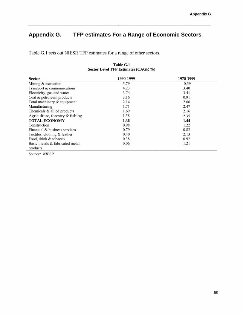
Appendix G

59

Appendix G. TFP estimates For a Range of Economic Sectors

Table G.1 sets out NIESR TFP estimates for a range of other sectors.

Table G.1

Sector Level TFP Estimates (CAGR %)

Sector 1990-1999 1970-1999 Mining & extraction 5.79 -0.59 Transport & communications 4.23 3.40 Electricity, gas and water 3.74 3.41 Coal & petroleum products 3.16 0.91 Total machinery & equipment 2.14 2.66 Manufacturing 1.71 2.47 Chemicals & allied products 1.69 2.16 Agriculture, forestry & fishing 1.58 2.35 TOTAL ECONOMY 1.36 1.44 Construction 0.98 1.22 Financial & business services 0.79 0.82 Textiles, clothing & leather 0.40 2.13 Food, drink & tobacco 0.38 0.92 Basic metals & fabricated metal products

0.06 1.21

Source: NIESR

Appendix H

60

Appendix H. Anticipated Input Price Changes and RPI

Our analysis set out in Section VI, shows that expected input price growth in the sewerage and water sector is greater than RPI growth, and therefore LE’s approach of setting X equal to water and sewerage sector TFP and ignoring input prices would not ex ante provide sufficient revenues to allow companies to finance their activities. This is consistent with a recent report for YWS by ICS Consulting, which to examined the impact of electricity price changes on RPI, and the overall impact of the change on YW’s ability to finance its activities.49 The reports authors concluded that the indexation of water companies’ revenues did not adequately compensate them for increases in power costs. This is because the water industry is relatively energy intensive, whereas the electricity component of RPI basket is relatively small. In particular, the authors noted: • Increases in domestic electricity prices feed into RPI directly (“first-order effects”). In

addition, increases in non-domestic electricity prices used by industrial and consumer (I&C) users to produce final goods feed through to increases in RPI. These are referred to as “second-order effects”.

• Combined, domestic and I&C charges constitute approximately 1.75% of the RPI basket. The authors calculate a combined first-order and second-order effect on the basis of Oxera’s forecast of energy prices of approximately 0.13% (in the first year).

• The study demonstrates that the increase in allowed revenues (through the RPI adjustment) fails to compensate water companies for increases in costs. Operating costs for Yorkshire water in the first year increase by approximately 1%, and therefore the overall increase in costs is greater than the compensating increase in revenues from RPI indexation. This divergence arises because the water industry is relatively energy intensive, compared to the economy as a whole.50

The YWS study demonstrates that it is necessary to allow for specific input price effects in setting allowed revenues because companies might not be adequately compensated through changes to RPI. Our approach to setting X and allowed revenues correctly compensates companies for input price changes. Starting with our initial definition of X below, we demonstrate that our approach

49 ICS Consulting Ltd (March 2004) RPI Indexation of Power Costs, A Report for Yorkshire Water 50 The short-fall in compensation to water companies will be compounded by expected lag effects. Increases in

wholesale charges are likely to feed into industrial user charges relatively quickly (depending on the nature of companies’ individual contracts). However, increases in allowed revenues through RPI increases might occur with a lag; this is because in setting prices Ofwat use a RPI calculated in the previous November.

Appendix H

61

allows industry revenues to increase in line with their input costs (specifically, there is no double counting with RPI, which cancel in our approach). Changes in allowed revenues (AR) under NERA’s approach are set equal to:

)IP - (IP-)TFP - (TFP -RPI X-RPIAR economyindustryeconomyindustry== Noting that RPI = IPeconomy – TFPeconomy, we have:51

RPI - IP TFP -RPI AR industryindustry += → industryindustry TFP-IP AR = That is, once the RPI indexation has taken place, allowed revenues will have been adjusted for sector input price changes and sector TFP change.

51 We note that in practice this relationship might not hold because of estimation error. We comment briefly

at the end of Section VI.E on the impact of estimation error on our forecast of efficiency.

NERA Economic Consulting 15 Stratford Place London W1C 1BE United Kingdom Tel: +44 20 7659 8500 Fax: +44 20 7659 8501 www.nera.com

estimating opex and capex efficiency - · pdf fileestimating opex and capex efficiency a final...

Documents