Public Economics

(Master PPD & APE, Paris School of Economics) T. Piketty

Academic year 2016-2017

Lecture 1: State formation & taxation in historical perspective

(check on line for updated versions)

Roadmap of lecture 1 • State formation & govt regulation in history • Standard economic rationales for taxes & transfers • Basic facts about taxes & transfers in rich countries • On the structure of taxes in EU countries • Basic facts about taxes in developing countries • Optimal policy: social objective vs incidence • Tax and transfer incidence: macro perspective • Tax and transfer incidence micro perspective

State formation & government regulation in historical perspective

• The objective of this course is to present an introduction to public economics, with special emphasis on the history of taxation, public spending and state formation, normative theories of government intervention & redistribution, and the incidence of tax and transfer policies, both in developed countries and in the developing world

• The rise of the fiscal and social state (taxes<10% of national income Y until WW1, vs. 30-50% Y in all rich countries today) is a crucial evolution that we will introduce today.

• This is a major social, economic and political transformation, which corresponds to a transition from minimal state to educational, developmental and welfare state.

• Throughout this course we will try to understand and analyze this evolution, both from an historical and normative viewpoint.

• Although this course will focus upon taxes and transfers, one should keep in mind that the rise of fiscal and social state represents only one aspect of the history of state formation and government regulation.

• The capital and democratic state (the set of legal rules and institutions governing property, labor and political relations between individuals) can be even more important than the fiscal system and public spendings, and in many ways encompasses the fiscal and social state. See Economic History course on:

• Basic civil & political rights: forced vs free labor, restrictions on mobility and occupational rights (major historical role)

• Property regimes: legal system shapes balance of power between owners & non-owners; public vs private property; workers rights & labor law (co-determination, unions); tenants rights & inheritance; intellectual property rights; monetary regimes & capital controls

• Family vs government roles: rules & norms regarding marriage, fertility, gender, education, etc.

• Political regimes and the organization of governement: electoral & party systems, nations-states, federations, empires

• During 21c, like in previous centuries, the evolution of fiscal & social institutions will be largely determined by the evolution of legal & political institutions (EU organization, participatory governance,etc.)

• In this course, we take a relatively narrow view of governement, i.e. we focus upon taxes and transfers and largely take other public institutions as given (in particular the property regime). But one should keep in mind that here are many different ways & dimensions to evaluate the structure & size of government.

• Exemple: should we look at share of govt tax revenues in national income Y, or at the share of govt property in national capital K?

China vs Europe: Chinese govt has smaller tax share in Y, but higher share in K ownership. Which state is most powerful?

Standard economic rationales for taxes & transfers • (1) Public good provision: raising tax revenue to finance public

goods (non-excludable): defense, roads, health, education, etc. • (2) Externalities: Pigouvian corrective tax and subsidy schemes so

to induce private agents to internalize external effects (e.g. global warming, carbon tax)

• (3) Stabilization: taxes & transfers can also serve as automatic stabilizers and reduce macroeconomic volatility (mostly a by-product of tax and transfer systems)

• (4) Redistribution: designing taxes & transfers in order to implement a fair distribution of income, wealth and welfare

• Rationales (1), (2), (3) = taxes/transfers generate “Pareto improvements” (i.e. everybody is better off) and correspond to failures of the “first welfare theorem” (= under certain assumptions, market equilibria are Pareto efficient)

• Rationale (4) = pure redistribution = taxes/transfers shift the economy to another Pareto optimum (i.e. some people are better off and some other people are worst off, e.g. poor vs rich)

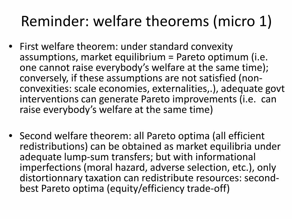
Reminder: welfare theorems (micro 1) • First welfare theorem: under standard convexity

assumptions, market equilibrium = Pareto optimum (i.e. one cannot raise everybody’s welfare at the same time); conversely, if these assumptions are not satisfied (non-convexities: scale economies, externalities,.), adequate govt interventions can generate Pareto improvements (i.e. can raise everybody’s welfare at the same time)

• Second welfare theorem: all Pareto optima (all efficient

redistributions) can be obtained as market equilibria under adequate lump-sum transfers; but with informational imperfections (moral hazard, adverse selection, etc.), only distortionnary taxation can redistribute resources: second-best Pareto optima (equity/efficiency trade-off)

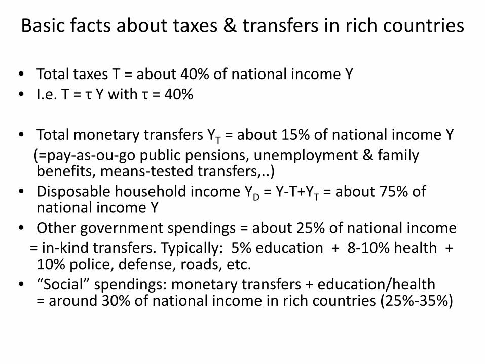
Basic facts about taxes & transfers in rich countries • Total taxes T = about 40% of national income Y • I.e. T = τ Y with τ = 40% • Total monetary transfers YT = about 15% of national income Y (=pay-as-ou-go public pensions, unemployment & family

benefits, means-tested transfers,..) • Disposable household income YD = Y-T+YT = about 75% of

national income Y • Other government spendings = about 25% of national income = in-kind transfers. Typically: 5% education + 8-10% health +

10% police, defense, roads, etc. • “Social” spendings: monetary transfers + education/health

= around 30% of national income in rich countries (25%-35%)

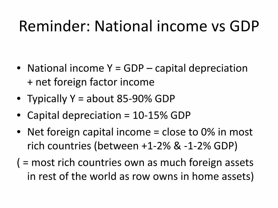
Reminder: National income vs GDP • National income Y = GDP – capital depreciation

+ net foreign factor income • Typically Y = about 85-90% GDP • Capital depreciation = 10-15% GDP • Net foreign capital income = close to 0% in most

rich countries (between +1-2% & -1-2% GDP) ( = most rich countries own as much foreign assets

in rest of the world as row owns in home assets)

• On long-run evolution of total tax revenues: in rich countries T/Y was less than 10% in the early 20c (police, defense, basic infrastructure and administration), rose enormously between 1950 & 1980, and then stabilized around 40% (with important variations between countries)

• On long-run of the structure of public spending, see

Lindert, Growing Public – Social spending & economic growth since the 18th century, CUP 2004

• For recent evolutions, see Adema et al, OECD 2011; see also Piketty-Saez HPE 2013 Table 1 : most of the rise in T/Y is due to the rise of social spendings (social transfers, education, health)

• I.e. the rise of the modern fiscal state corresponds to the rise of the social state

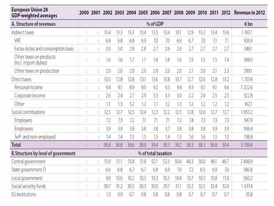
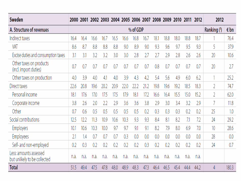
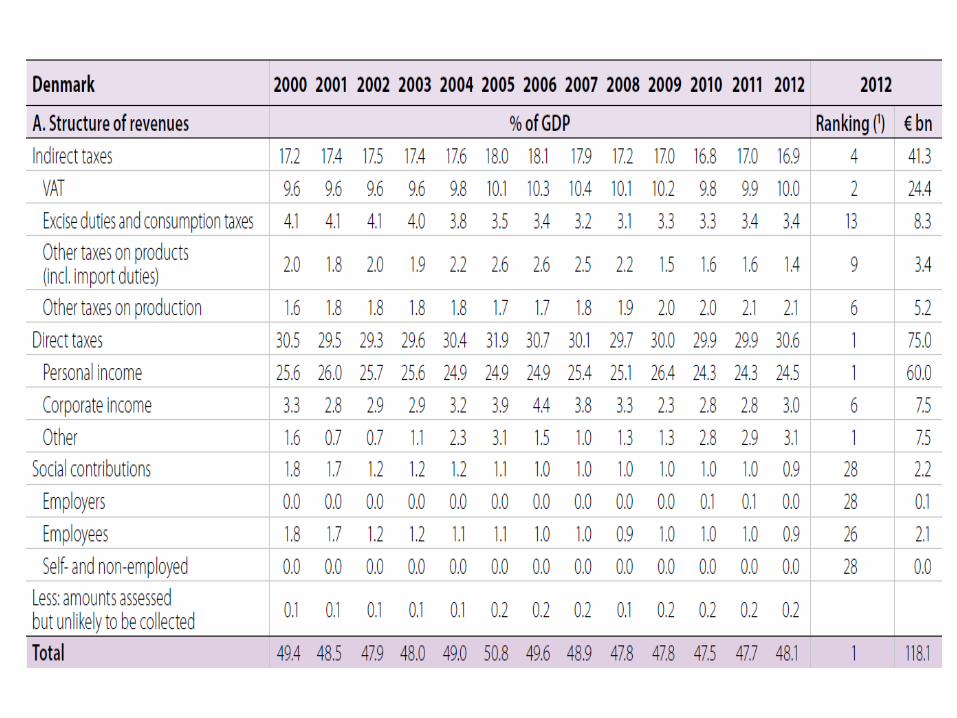
On the structure of taxes in Europe • On structure of taxes in Europe, see “Taxation Trends in the

European Union”, Eurostat 2014 (summary); see also Eurostat 2013; see also updated tables on taxation trends website

• Typically: T = 1/3 indirect taxes + 1/3 direct taxes + 1/3 social contributions

• But: large variations between EU countries • And: this decomposition is not really meaningful; what matters

is the factor income decomposition (capital vs labor) and the consumption vs saving decomposition → see below on tax incidence

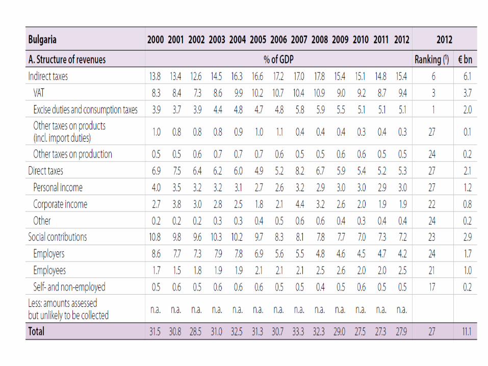
• Large variations in tax levels: see rich vs poor EU countries • Large variations in tax mix: EU 28 vs France, Germany, Denmark,

Sweden, Bulgaria • Large variations in tax regimes also correspond to large

variations in welfare state regimes: see Esping Andersen, The Three Worlds of Welfare Capitalism, PUP 1990 : Bismarck vs Beveridge vs Nordic models of welfare state organization

Basic facts about taxes and transfers in developing countries

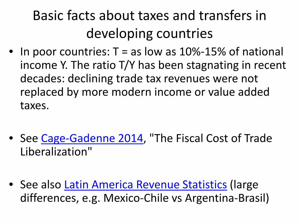
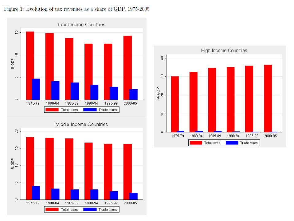
• In poor countries: T = as low as 10%-15% of national income Y. The ratio T/Y has been stagnating in recent decades: declining trade tax revenues were not replaced by more modern income or value added taxes.

• See Cage-Gadenne 2014, "The Fiscal Cost of Trade

Liberalization"

• See also Latin America Revenue Statistics (large differences, e.g. Mexico-Chile vs Argentina-Brasil)

Optimal tax policy: social objective vs tax and transfer incidence

• How can we formulate the problem of socially optimal tax and transfer policy?

• One needs to specify the social objective: « maximin » redistributive objective (maximize welfare of individuals with minimal welfare level) (≈ minimize poverty), output maximization (no redistributive objective at all), etc.

→ see Lecture 2 • And one needs to analyze the incidence of taxes & transfers:

i.e. what is the impact of taxes and transfers on economic transactions, supply and demand, prices, etc.; key question: at the end of the day, who pays what, and who receives what?

→ see today for an introduction to the pb of tax incidence, and see Lectures 3-7 for more precise analysis in the case of taxes on income, wealth and carbon

Tax & transfer incidence: macro approach • Tax incidence problem = the central issue of public

economics = who pays what? • General principle: it depends on the various elasticities

of demand and supply on the relevant labor market, capital market and goods market.

• Usually the more elastic tax benefit wins, i.e. the more elastic tax base shifts the tax burden towards the less elastic

• Same pb with transfer incidence: who benefits from housing subsidies: tenants or landlords? – this depends on elasticities

• Opening up the black box of national accounts tax aggregates is a useful starting point in order to study factor incidence (macro approach)

• But this needs to be supplemented by micro studies

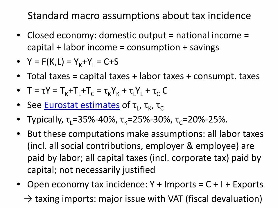
Standard macro assumptions about tax incidence

• Closed economy: domestic output = national income = capital + labor income = consumption + savings

• Y = F(K,L) = YK+YL = C+S • Total taxes = capital taxes + labor taxes + consumpt. taxes • T = τY = TK+TL+TC = τKYK + τLYL + τC C • See Eurostat estimates of τL, τK, τC • Typically, τL=35%-40%, τK=25%-30%, τC=20%-25%. • But these computations make assumptions: all labor taxes

(incl. all social contributions, employer & employee) are paid by labor; all capital taxes (incl. corporate tax) paid by capital; not necessarily justified

• Open economy tax incidence: Y + Imports = C + I + Exports → taxing imports: major issue with VAT (fiscal devaluation)

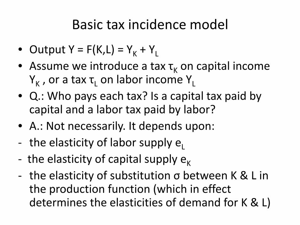
Basic tax incidence model

• Output Y = F(K,L) = YK + YL • Assume we introduce a tax τK on capital income

YK , or a tax τL on labor income YL • Q.: Who pays each tax? Is a capital tax paid by

capital and a labor tax paid by labor? • A.: Not necessarily. It depends upon: - the elasticity of labor supply eL

- the elasticity of capital supply eK - the elasticity of substitution σ between K & L in

the production function (which in effect determines the elasticities of demand for K & L)

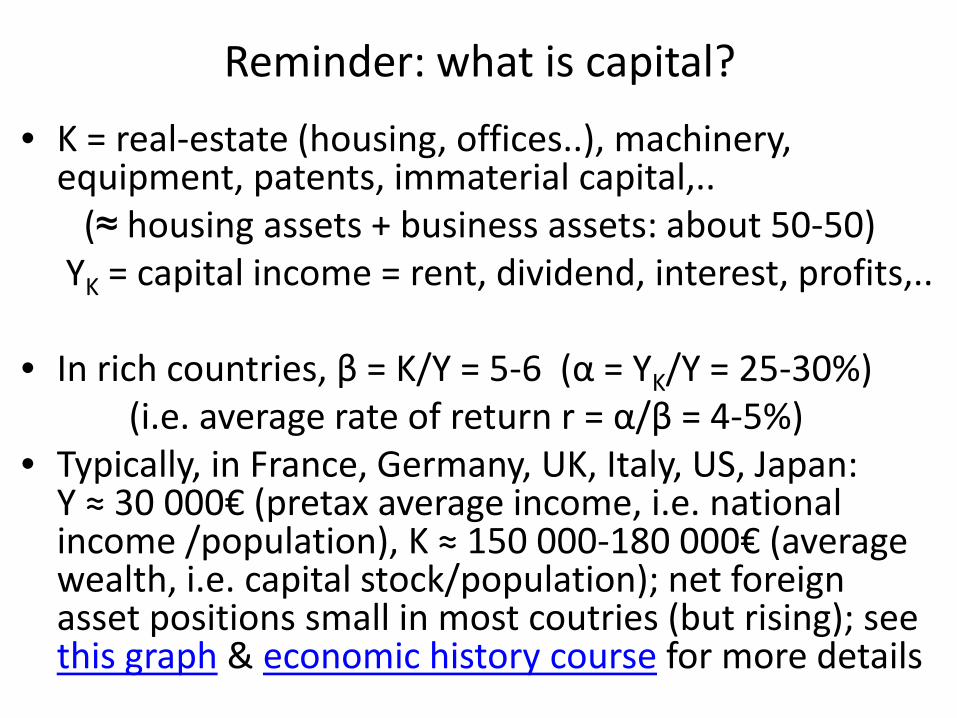
Reminder: what is capital? • K = real-estate (housing, offices..), machinery,

equipment, patents, immaterial capital,.. (≈ housing assets + business assets: about 50-50) YK = capital income = rent, dividend, interest, profits,.. • In rich countries, β = K/Y = 5-6 (α = YK/Y = 25-30%) (i.e. average rate of return r = α/β = 4-5%) • Typically, in France, Germany, UK, Italy, US, Japan:

Y ≈ 30 000€ (pretax average income, i.e. national income /population), K ≈ 150 000-180 000€ (average wealth, i.e. capital stock/population); net foreign asset positions small in most coutries (but rising); see this graph & economic history course for more details

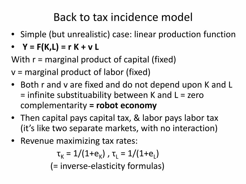
Back to tax incidence model • Simple (but unrealistic) case: linear production function • Y = F(K,L) = r K + v L With r = marginal product of capital (fixed) v = marginal product of labor (fixed) • Both r and v are fixed and do not depend upon K and L

= infinite substituability between K and L = zero complementarity = robot economy

• Then capital pays capital tax, & labor pays labor tax (it’s like two separate markets, with no interaction)

• Revenue maximizing tax rates: τK = 1/(1+eK) , τL = 1/(1+eL) (= inverse-elasticity formulas)

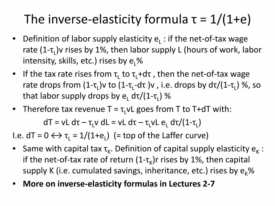
The inverse-elasticity formula τ = 1/(1+e) • Definition of labor supply elasticity eL : if the net-of-tax wage

rate (1-τL)v rises by 1%, then labor supply L (hours of work, labor intensity, skills, etc.) rises by eL%

• If the tax rate rises from τL to τL+dτ , then the net-of-tax wage rate drops from (1-τL)v to (1-τL-dτ )v , i.e. drops by dτ/(1-τL) %, so that labor supply drops by eL dτ/(1-τL) %

• Therefore tax revenue T = τLvL goes from T to T+dT with: dT = vL dτ – τLv dL = vL dτ – τLvL eL dτ/(1-τL) I.e. dT = 0 ↔ τL = 1/(1+eL) (= top of the Laffer curve) • Same with capital tax τK. Definition of capital supply elasticity eK :

if the net-of-tax rate of return (1-τK)r rises by 1%, then capital supply K (i.e. cumulated savings, inheritance, etc.) rises by eK%

• More on inverse-elasticity formulas in Lectures 2-7

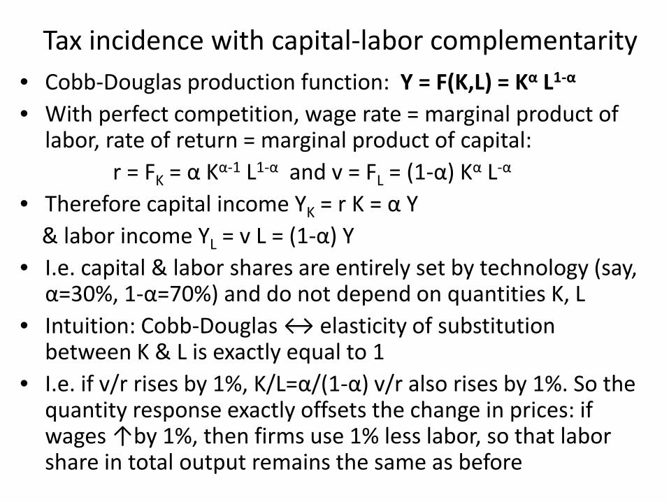
Tax incidence with capital-labor complementarity • Cobb-Douglas production function: Y = F(K,L) = Kα L1-α • With perfect competition, wage rate = marginal product of

labor, rate of return = marginal product of capital: r = FK = α Kα-1 L1-α and v = FL = (1-α) Kα L-α • Therefore capital income YK = r K = α Y & labor income YL = v L = (1-α) Y • I.e. capital & labor shares are entirely set by technology (say,

α=30%, 1-α=70%) and do not depend on quantities K, L • Intuition: Cobb-Douglas ↔ elasticity of substitution

between K & L is exactly equal to 1 • I.e. if v/r rises by 1%, K/L=α/(1-α) v/r also rises by 1%. So the

quantity response exactly offsets the change in prices: if wages ↑by 1%, then firms use 1% less labor, so that labor share in total output remains the same as before

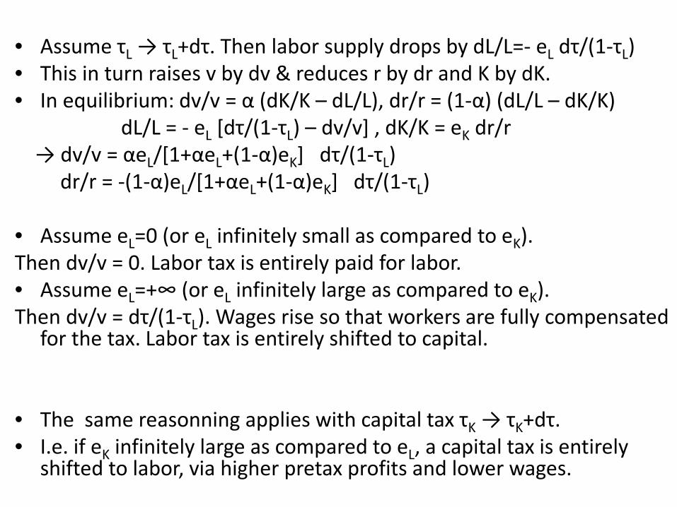
• Assume τL → τL+dτ. Then labor supply drops by dL/L=- eL dτ/(1-τL) • This in turn raises v by dv & reduces r by dr and K by dK. • In equilibrium: dv/v = α (dK/K – dL/L), dr/r = (1-α) (dL/L – dK/K) dL/L = - eL [dτ/(1-τL) – dv/v] , dK/K = eK dr/r → dv/v = αeL/[1+αeL+(1-α)eK] dτ/(1-τL) dr/r = -(1-α)eL/[1+αeL+(1-α)eK] dτ/(1-τL) • Assume eL=0 (or eL infinitely small as compared to eK). Then dv/v = 0. Labor tax is entirely paid for labor. • Assume eL=+∞ (or eL infinitely large as compared to eK). Then dv/v = dτ/(1-τL). Wages rise so that workers are fully compensated

for the tax. Labor tax is entirely shifted to capital. • The same reasonning applies with capital tax τK → τK+dτ. • I.e. if eK infinitely large as compared to eL, a capital tax is entirely

shifted to labor, via higher pretax profits and lower wages.

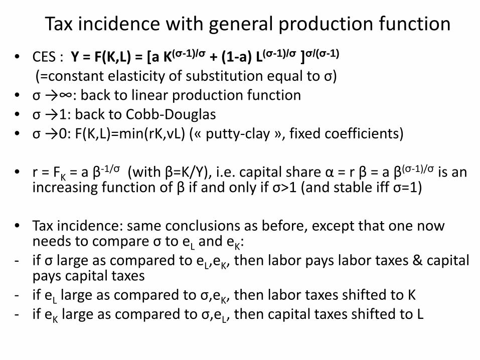
Tax incidence with general production function • CES : Y = F(K,L) = [a K(σ-1)/σ + (1-a) L(σ-1)/σ ]σ/(σ-1)

(=constant elasticity of substitution equal to σ) • σ →∞: back to linear production function • σ →1: back to Cobb-Douglas • σ →0: F(K,L)=min(rK,vL) (« putty-clay », fixed coefficients) • r = FK = a β-1/σ (with β=K/Y), i.e. capital share α = r β = a β(σ-1)/σ is an

increasing function of β if and only if σ>1 (and stable iff σ=1) • Tax incidence: same conclusions as before, except that one now

needs to compare σ to eL and eK: - if σ large as compared to eL,eK, then labor pays labor taxes & capital

pays capital taxes - if eL large as compared to σ,eK, then labor taxes shifted to K - if eK large as compared to σ,eL, then capital taxes shifted to L

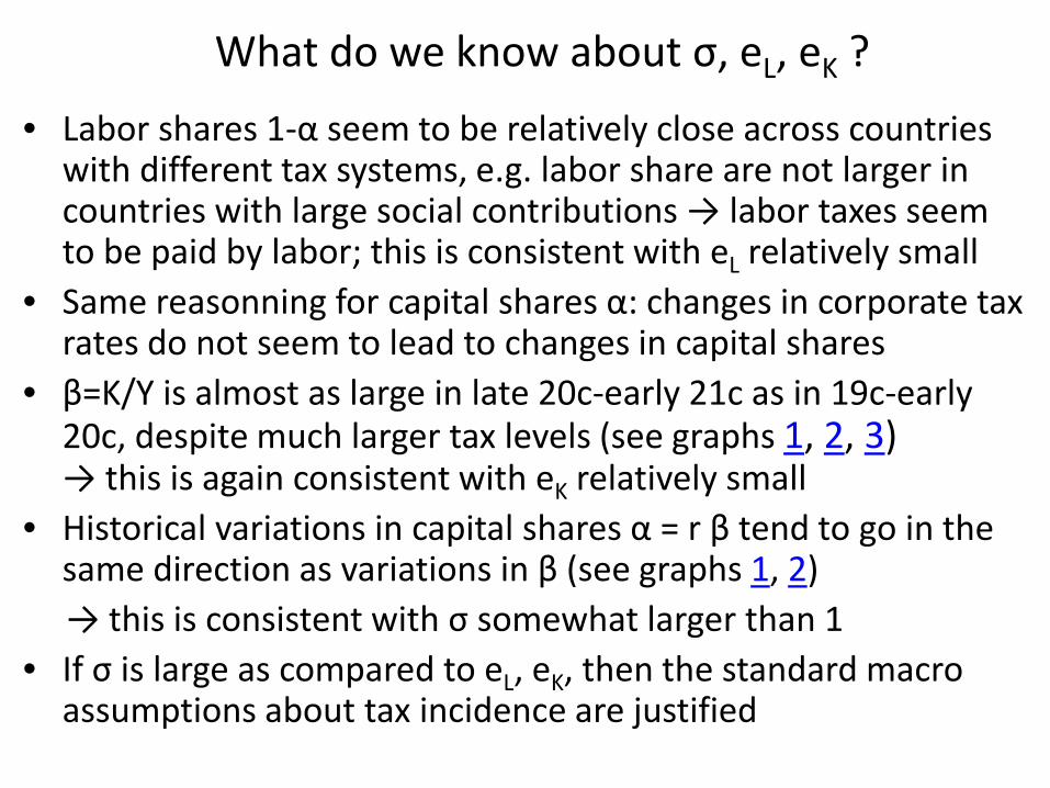
What do we know about σ, eL, eK ?

• Labor shares 1-α seem to be relatively close across countries with different tax systems, e.g. labor share are not larger in countries with large social contributions → labor taxes seem to be paid by labor; this is consistent with eL relatively small

• Same reasonning for capital shares α: changes in corporate tax rates do not seem to lead to changes in capital shares

• β=K/Y is almost as large in late 20c-early 21c as in 19c-early 20c, despite much larger tax levels (see graphs 1, 2, 3) → this is again consistent with eK relatively small

• Historical variations in capital shares α = r β tend to go in the same direction as variations in β (see graphs 1, 2)

→ this is consistent with σ somewhat larger than 1 • If σ is large as compared to eL, eK, then the standard macro

assumptions about tax incidence are justified

• But these conclusions are relatively uncertain: it is difficult to estimate macro elasticities

• Also they are subject to change. E.g. it is possible that σ tends to rise over the development process. I.e. σ<1 in rural societies where capital is mostly land (see Europe vs America: more land in volume in New world but less land in value; price effect dominates volume effects: σ<1). But in 20c & 21c, more and more uses for capital, more substitution: σ>1. Maybe even more so in the future. Capital is multidimensional: σ varies.

• Elasticities do not only reflect real economic responses. E.g. eK can be large for pure accounting/tax evasion reasons: even if capital does not move, accounts can move. Without fiscal coordination between countries (unified corporate tax base, automatic exchange of bank information,..), capital taxes might be more and more shifted to labor.

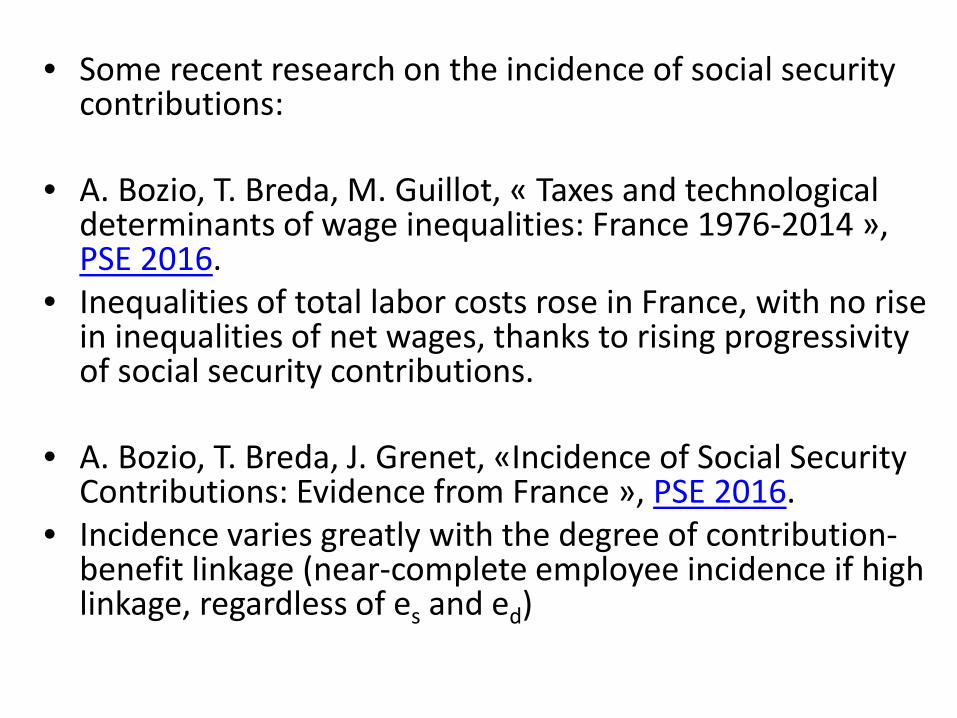
• Some recent research on the incidence of social security contributions:

• A. Bozio, T. Breda, M. Guillot, « Taxes and technological

determinants of wage inequalities: France 1976-2014 », PSE 2016.

• Inequalities of total labor costs rose in France, with no rise in inequalities of net wages, thanks to rising progressivity of social security contributions.

• A. Bozio, T. Breda, J. Grenet, «Incidence of Social Security

Contributions: Evidence from France », PSE 2016. • Incidence varies greatly with the degree of contribution-

benefit linkage (near-complete employee incidence if high linkage, regardless of es and ed)

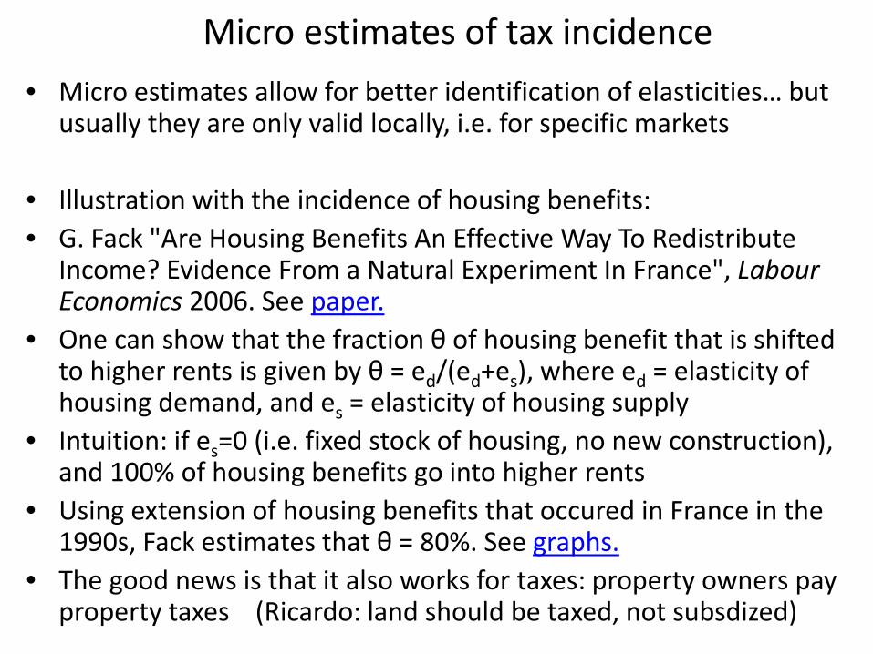
Micro estimates of tax incidence • Micro estimates allow for better identification of elasticities… but

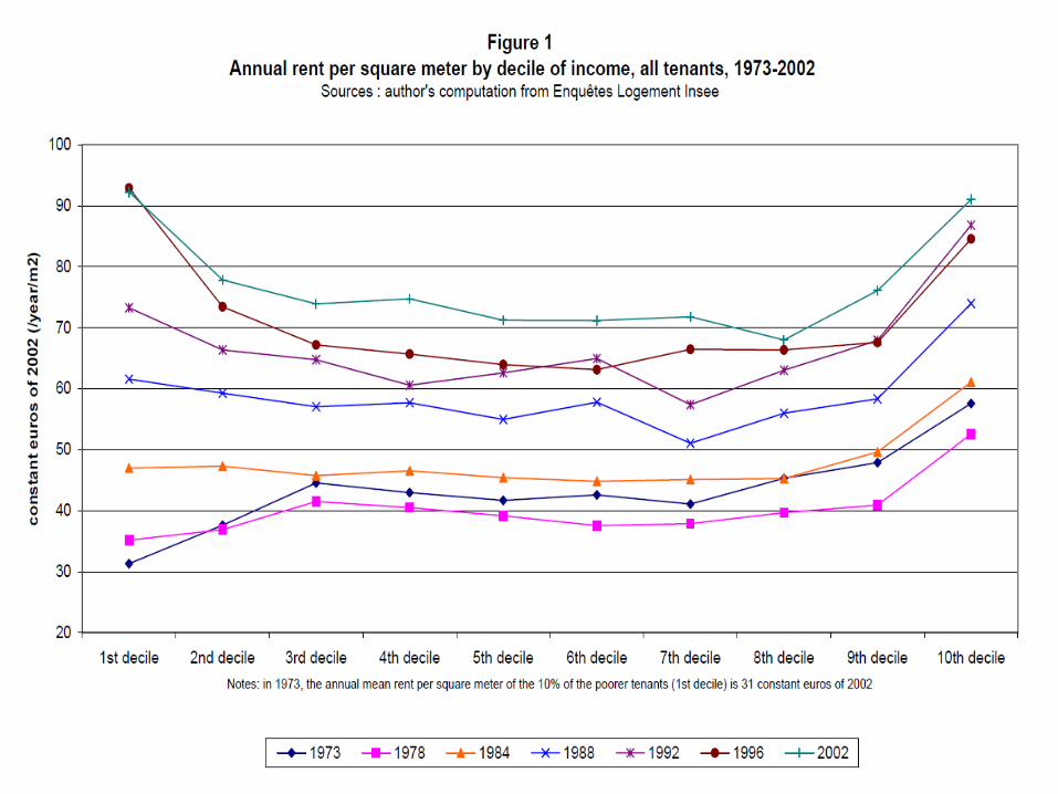
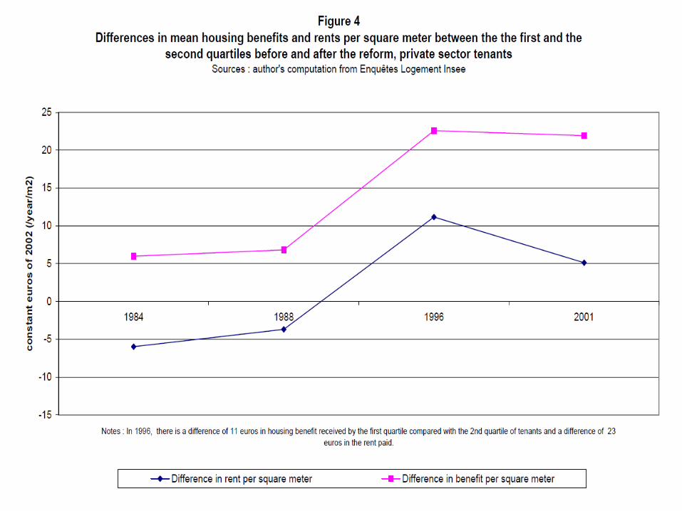
usually they are only valid locally, i.e. for specific markets • Illustration with the incidence of housing benefits: • G. Fack "Are Housing Benefits An Effective Way To Redistribute

Income? Evidence From a Natural Experiment In France", Labour Economics 2006. See paper.

• One can show that the fraction θ of housing benefit that is shifted to higher rents is given by θ = ed/(ed+es), where ed = elasticity of housing demand, and es = elasticity of housing supply

• Intuition: if es=0 (i.e. fixed stock of housing, no new construction), and 100% of housing benefits go into higher rents

• Using extension of housing benefits that occured in France in the 1990s, Fack estimates that θ = 80%. See graphs.

• The good news is that it also works for taxes: property owners pay property taxes (Ricardo: land should be taxed, not subsdized)

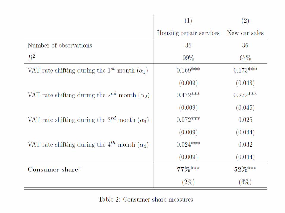
• Illustration with the incidence of value added taxes (VAT): • C. Carbonnier, “Who Pays Sales Taxes ? Evidence from French VAT

Reforms, 1987-1999”, Journal of Public Economics 2007. See paper. • Q.: Is the VAT a pure consomption tax? Not so simple • First complication. Valued added = output – intermediate

consumption = wages + profits. I.e. value added = Y = YK + YL = C + S • So is the VAT like an income tax on YK + YL ? No, because investment

goods are exempt from VAT, and I = S in closed economy • Second complication. Even if VAT was a pure tax on C, this does not

mean that it entirely shifted on consumer prices. VAT is always partly shifted on prices and partly shifted on factor income (wages & profits). How much exactly depends on the supply & demand elasticities for each specific good or service.

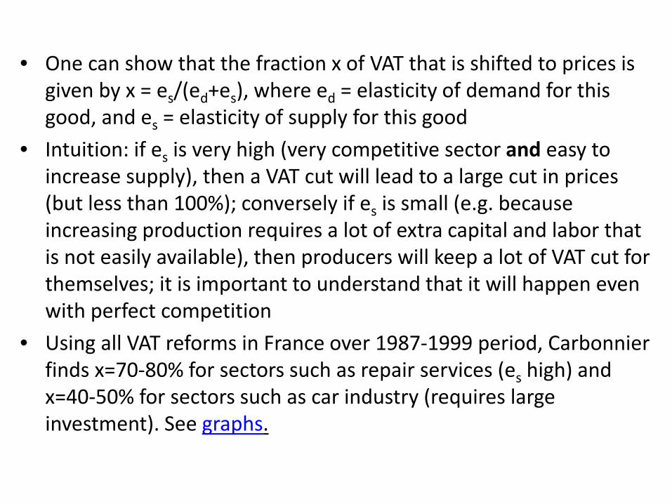
• One can show that the fraction x of VAT that is shifted to prices is

given by x = es/(ed+es), where ed = elasticity of demand for this good, and es = elasticity of supply for this good

• Intuition: if es is very high (very competitive sector and easy to increase supply), then a VAT cut will lead to a large cut in prices (but less than 100%); conversely if es is small (e.g. because increasing production requires a lot of extra capital and labor that is not easily available), then producers will keep a lot of VAT cut for themselves; it is important to understand that it will happen even with perfect competition

• Using all VAT reforms in France over 1987-1999 period, Carbonnier finds x=70-80% for sectors such as repair services (es high) and x=40-50% for sectors such as car industry (requires large investment). See graphs.