Public de�cit sustainability, public debt and

monetization in an endogenous growth model: an

application for Turkey

Özgür Kaan ERERDEM∗

March 15, 2010

Very Preliminary Version

Abstract

This paper analyzes the long term sustainability of budgetary policies in a generalequilibrium framework. The analysis is based on an overlapping generations model wherethe government �xes a tax rate on factor incomes, conducts unproductive and productivepublic spendings and determines the weight of public bonds issuance and monetizationin de�cit �nancing. A budgetary rule setting the economy on a balanced growth pathis considered sustainable. The model is used to evaluate the sustainability of Turkishbudgetary policies since 1980. The results show that Turkish budgetary policies becamesustainable in the period 1999-2007. Alternative policy simulations show that Turkeycould have conducted more expansionnist budget policies without risking sustainabilityduring this period. The model shows also that the negative impact of in�ation tax onprivate capital accumulation is greater than the impact of factor income tax.

1 INTRODUCTION

Several works in economics litterature has studied public �nance issues using economicgrowth models. Chalk (2000) and Rankin and Ro�a (2003) a�rm, using exogenousgrowth models, that public debt sustainability requires low initial public debt and pub-lic de�cit ratios. Futagami and Shibata (2003) �nd the same result with an endogenousgrowth model. Bräuninger (2005) analyzes public debt sustainability using an endogenousgrowth model within an overlapping generations (OLG) setting. He studies the impact ofdi�erent budgetary rules and concludes that above a public de�cit/GDP ratio threshold,the budgetary policy becomes unsustainable, as there are no more balanced growth paths.Furthermore, there exists a threshold of initial public debt/private capital ratio abovewhich the economy can not reach a balanced growth path. On the other hand, the studyof Bräuninger assumes only non-productive public spendings. Arai (2008) and Yakita(2008) develop this approach by incorporating productive public spendings. Within anOLG setting, Arai assumes (2008) public spendings as a �ow, as in Barro (1990). He

∗LEDa, Université Paris-Dauphine

1

demonstrates that for low initial values, increasing public spendings allows sustainabil-ity because its positive impact on production exceeds the negative impact on costs. InYakita (2008), public spendings �nance a public capital stock, as in Futagami, Moritaand Shibata (1993). He concentrates the analysis on the "golden rule" of public �nancewhich consists of issuing debt only for public investments. As in Bräuninger, he �ndsthe existence of a public debt threshold, for each level of public capital, above which thebudgetary policy is unsustainable in the long run.

The model developed in this paper is inspired by Yakita (2008). It contains two maindi�erences: it includes money as an assett and it considers public de�cit as an endoge-nous variable. In our model, the government intervenes in the economy in several ways.It realizes productive and unproductive public spendings, and collects taxes on factorincome. These three exogenous parameters are expressed as a share in GDP. The publicde�cit generated by this policy is �nanced with public bonds and money creation. Thegovernment �xes the share of each �nancing method. Thus the government decides aboutfour policy parameters. Fixed policy rules that enables the economy to reach a balancedgrowth path are considered sustainable.

In the model, money supply is represented by money creation aiming at �nancingthe public de�cit. Thus, money supply consists of seignorage. Money demand is rep-resented by a Clower (1967) type liquidity constraint. Initially, this constraint assumesthat agents have to �nance the whole of their consumpton with money, and thus haveto hold money before the transaction. In an overlapping generations setting, such anassumption would block savings and consequently the private capital accumulation. Thisis why we will adopt the approach of Lucas and Stokey (1987) who distinguish goodsbought with money and with credit. We will then assume, as in Hahn and Solow (1995),a partial liquidity constraint forcing old agents to realize a �xed portion of their spendingsusing money. In other terms, young agents are forced to hold cash balances in order torealize a �xed portion of their future consumption with monet. This way we obtain aliquidity constraint1 that creates distorsions on capital accumulation without blocking itcompletely.

The introduction of money allows to take into account the transaction costs createdby the need of holding money. The latter blocks a portion of the funds that could havebeen invested in other assetts as public bonds or private capital. Money in�uences thenthe economic equilibrium and dynamics of accumulation (Crettez, Michel et Wigniolle1999). Money supply being limited to monetization, the model enables to visualize in�a-tion tax.

For the case of Turkey, public �nance sustainability has been mostly analyzed in em-pirical works2. On the other hand, Yeldan (2002), analyzes the impact of Turkish bud-getary policies conducted since 2000, with the support of the IMF, by using a theoreticalendogenous growth model. The latter assumes an OLG setting where the governmentmake public investments in the domain of education. He realizes a computable genralequilibrium analysis which concludes that the budgetary policies implemented with theIMF are too restrictive and deprive the economy of funds needed to improve the quality

1For a detailed analysis of cash-in-advance models, see Villieu (1992).2See Akçay, Alper and Özmucur (2002), Merola (2006) and Gürbüz, Jobert and Tuncer (2007)

2

of workforce through education policies.

The simulations of our model show that Turkish budgetary policies conducted in 1980-1988 and 1989-1998 periods were unsustainable. In other words they do not allow theeconomy to reach a balance growth path. However, the policy of the 1999-2007 periodis sustainable. On the other hand, alternative policy simulations concludes that moreexpansionist and growth enhancing budgetary policies could have been implemented inTurkey in this period, without breaching sustainability in the long run. Our results arethen similar to that of Yeldan (2002).

In order to better illustrate the impact of monetization, we simulate alternative poli-cies also for the 1980-1988 where initially the budgetary policy was unsustainable. Theobjective is to compare the equilibria obtained with di�erent stabilization measures.Results show that sustainability achieved by tax increases enables more growth thansustainability reached through monetization, in other terms, through in�ation tax. Thelatter has a larger negative impact on private capital accumulation than direc taxes.

The paper is organized as follows: section II presents the model. Section III displaysaccumulation dynamics and de�nes public �nance sustainability. Section IV shows theresults of the simulations on Turkish budget policies. The last section concludes.

2 THE MODEL

2.1 Consumers

We consider an overlapping generations model (OLG). Two generations of agents coexistat each date t. Each agent lives only two periods. Agents are not altruist, thus we assumethat there are no bequests. The anticipations of agents are perfect.

An agent born at period t maximizes the intertemporal utility function given by :

U = ln(cj,t) + β ln(cv,t+1) (1)

In equation (1), cj,t stands for the consumption of the young agent at date t. cv,t+1

represents the consumption of this same agent during retirement in period t + 1. Thevariable β is the psychological discount factor re�ecting the relative preference of theagent for present consumption. Agents are supposed to have a relative preference forpresent consumption, thus we assume 0 < β < 1.

Agents work only during youth. Their labor supply is assumed to be exogenous andinelastic. We assume that there is no demographic growth and the active population'ssize is normalized to 1. Thus, from now on, we pursue the analysis considering that ateach period one young and one old agent co-exist.

The wage wt is the only source of revenue of an agent. We assume that the governmentdetermines a �xed tax rate θ on production factor incomes. Consequently, the wage rateis taxed and the disposable revenue of an agent is (1−θ)wt. This revenue is split between

3

present consumption cj,t, real non-monetary savings st, and real cash balances Mt+1

Pt. The

budget constraint of a young agent is then :

cj,t = (1− θ)wt − st −Mt+1

Pt(2)

The consumer agent born in period t becomes old in t+1, stops working and consumesthe real non-monetary savings and real cash balances. The interest rate being also taxed,the non-monetary savings realized during youth yields (1 + (1− θ)rt+1) st at t + 1. Inaddition to this non-monetary savings income, the old agent spends also his cash balanceswhose real value becomes Mt+1

Pt+1, following the modi�cation of prices between period t and

t+ 1. The budget constraint of the old agent in t+ 1 is :

cv,t+1 = (1 + (1− θ)rt+1) st +Mt+1

Pt+1(3)

For simpli�cation purposes, we denote as Rt+1 the real detaxed return on non-monetary savings, and as mt+1 the real cash balances hold in t for consumption in t+ 1.These two variables are de�ned in the following way :

Rt+1 = (1 + (1− θ)rt+1) (4)

mt+1 =Mt+1

Pt(5)

An agent born in t saves money whose nominal value is Mt+1. We prefer to use theindex t+ 1 instead of t because this amount will be spent in period t+ 1 by this agent.

The agent faces a cash-in-advance constraint à la Hahn and Solow (1995). A �xedportion µ of future consumption is realized using money. The liquidity constraint iswritten in the following way:

µPt+1cv,t+1 ≤Mt+1 (6)

The return of money is supposed to be lower than that of non-monetary savings3

( PtPt+1

< Rt+1). Money assures less return than non-monetary savings. That's whyagents do not hold money more than the portion µ imposed by the liquidity constraint.The liquidity constraint is then binding:

µPt+1cv,t+1 = Mt+1 (7)

We develop the retired agents budget contraint given by (3) by including the cash-in-advance constraint (7) :

cv,t+1 =Rt+1st1− µ

(8)

3This assumption will be veri�ed at the steady state

4

The liquidity constraint (7) can be written, by dividing both sides of the equation byPt :

mt+1 = µπt+1cv,t+1 (9)

where πt+1 stands for the in�ation factor(Pt+1

Pt

)between t and t+ 1.

We include the liquidity constraint in the young agent's budget constraint by replacingthe expression of real balances mt+1 �guring in (2) by the one given in equation (9) :

cj,t = (1− θ)wt − st − µπt+1cv,t+1 (10)

By eliminating the non-monetary savings variable st in the modi�ed budget con-straints of retirement period (8) and active period (10), we obtain the intertemporalbudget constraint of an agent born in t :

cj,t = (1− θ)wt − cv,t+11− µRt+1

− cv,t+1µπt+1 (11)

This expression can be written in the following way:

cj,t = (1− θ)wt − cv,t+1

(1− µRt+1

+ µπt+1

)(12)

In the intertemporal budget constraint (12), the expression(

1−µRt+1

+ µπt+1

)repre-

sents the discount rate which takes into account the return on total savings (st +Mt+1

Pt).

A portion (1− µ) of future consumption is discounted using the real return Rt+1, whilethe portion µ left is discounted using the return on money 1

πt+1.

The consumer decides about consumption levels during youth cj,t, and retirementcv,t+1, and about non-monetary savings st, by maximizing the intertemporal utility func-tion (1) with respect to the intertemporal budget constraint (12):

{Max U(cj,t, cv,t+1)s.c. cj,t = (1− θ)wt − cv,t+1

(1−µRt+1

− µπt+1

)The resolution of this program yields the following results :

st =β(1− µ)(1− θ)wt

(1 + β)(1− µ+ µπt+1Rt+1)(13)

cj,t =(1− θ)wt

1 + β(14)

cv,t+1 =β(1− θ)wtRt+1

(1 + β)(1− µ+ µπt+1Rt+1)(15)

5

2.2 Production

We assume that �rms produce one good serving both for consumption and investment,using private capital Kt, labor Lt. In our model, public capital Gt enters the productionfunction, thus a�ects the level of production. In the same way as Yakita (2008), weassume that the production technology of a �rm i is given by the following Cobb-Douglasproduction function:

Yi,t = A Kαi,t (Gt Li,t)1−α (16)

with 0 < α < 1 and A > 0

The variable Gt represents the public capital stock and acts as a positive externalityon individual production of �rms. In the individual level, Gt is an exogenous variable,identical for all �rms. In the aggregate level, public capital becomes an endogenous vari-able, whose level is determined by budget policies. Public capital can be thought as theinfrastructure of an economy which permits �rms to produce.

Labor supply is exogenous, inelastic and normalized to 1 (Lt = 1). Under the hy-pothesis of perfect competition, marginal productivities of production factors are equalto their net utilisation costs. Denoting δ as the depreciation rate of both private andpublic capital, we write the interest rate rt and the wage rate wt in the following way:

rt + δ =∂Yi,t∂Ki,t

⇒ rt = αYi,tKi,t− δ (17)

wt =∂Yi,t∂Li,t

⇒ wt = (1− α)Yi,t (18)

2.3 Government

Government intervenes in the economy using the following instruments: unproductivepublic spendings, public investment spendings, taxes, �nancing of the public de�cit bymonetization and/or public bonds.

The public investment level of a period t is �xed proportionally to the GDP of theeconomy. We denote as i the weight of public investments in GDP. Thus, the amount ofpublic investments in a period t is denoted as iYt.

The amount of unproductive public spendings is also expressed proportionnally tothe GDP. The weight of these spendings in GDP is denoted g. Thus, the amount ofunproductive public spending in a period t is gYt.

The factor incomes are subject to the tax rate θ. Denoting as Bt the public bondsstock reimbursed at the end of period t, the total �scal revenue of the government inperiod t is :

Tt = θwtLt + θrtKt + θrtBt (19)

We replace the variables wt and rt by their expressions shown in (18) et (17). Giventhat we have Lt = 1, the �scal revenue becomes:

6

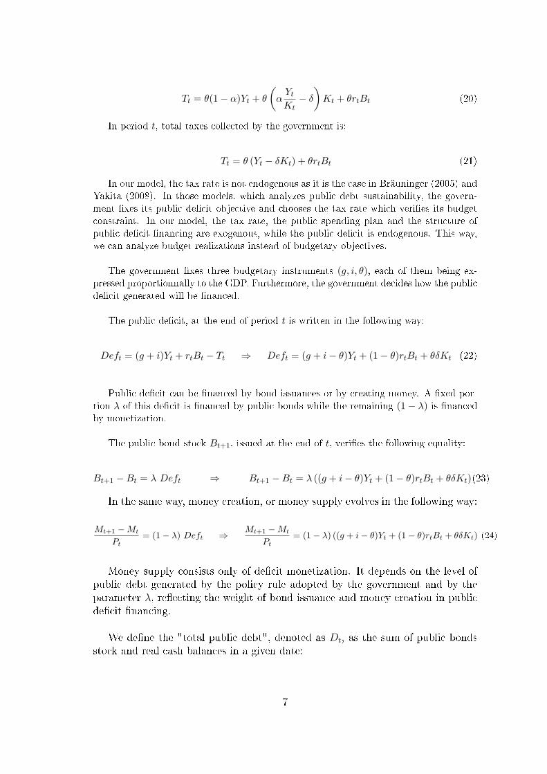
Tt = θ(1− α)Yt + θ

(αYtKt− δ)Kt + θrtBt (20)

In period t, total taxes collected by the government is:

Tt = θ (Yt − δKt) + θrtBt (21)

In our model, the tax rate is not endogenous as it is the case in Bräuninger (2005) andYakita (2008). In those models, which analyzes public debt sustainability, the govern-ment �xes its public de�cit objective and chooses the tax rate which veri�es its budgetconstraint. In our model, the tax rate, the public spending plan and the structure ofpublic de�cit �nancing are exogenous, while the public de�cit is endogenous. This way,we can analyze budget realizations instead of budgetary objectives.

The government �xes three budgetary instruments (g, i, θ), each of them being ex-pressed proportionnally to the GDP. Furthermore, the government decides how the publicde�cit generated will be �nanced.

The public de�cit, at the end of period t is written in the following way:

Deft = (g + i)Yt + rtBt − Tt ⇒ Deft = (g + i− θ)Yt + (1− θ)rtBt + θδKt (22)

Public de�cit can be �nanced by bond issuances or by creating money. A �xed por-tion λ of this de�cit is �nanced by public bonds while the remaining (1− λ) is �nancedby monetization.

The public bond stock Bt+1, issued at the end of t, veri�es the following equality:

Bt+1 −Bt = λ Deft ⇒ Bt+1 −Bt = λ ((g + i− θ)Yt + (1− θ)rtBt + θδKt)(23)

In the same way, money creation, or money supply evolves in the following way:

Mt+1 −Mt

Pt= (1− λ) Deft ⇒ Mt+1 −Mt

Pt= (1− λ) ((g + i− θ)Yt + (1− θ)rtBt + θδKt) (24)

Money supply consists only of de�cit monetization. It depends on the level ofpublic debt generated by the policy rule adopted by the government and by theparameter λ, re�ecting the weight of bond issuance and money creation in publicde�cit �nancing.

We de�ne the "total public debt", denoted as Dt, as the sum of public bondsstock and real cash balances in a given date:

7

Dt+1 = Bt+1 +Mt+1

Pt(25)

Dt = Bt +Mt

Pt−1

(26)

The evolution of public debt is obtained by taking the di�erence between thetwo expressions above. By simple manipulations, we write the dynamics of publicdebt:

Dt+1 −Dt = Bt+1 −Bt +Mt+1 −Mt

Pt− Mt

Ptρt (27)

with ρt representing the in�ation rate Pt−Pt−1

Pt−1. In the dynamic given in (27), we

can see the two public de�cit �nancing instruments: public bonds issues (Bt+1 −Bt)

and monetization(Mt+1−Mt

Pt

). In addition to these two mechanisms, the public debt

dynamic includes the expression Mt

Ptρt. By developing ρt in the latter, we obtain

Mt

Pt−1− Mt

Pt. This expression corresponds to the di�erence between the values of real

balances following an in�ation between t− 1 and t. This erosion generated by thein�ation is de�ned in the litterature as the in�ation tax.

Taking into account the dynamics (23), (24) and (27), we �nalize the develop-ment of the public debt accumulation :

Dt+1 −Dt = (g + i− θ)Yt + (1− θ)rtBt + θδKt −mt

(1− 1

πt

)(28)

Public investments, denoted as iYt, adds up to the existing (depreciated) publiccapital stock and assures its accumulation:

Gt+1 = (1− δ)Gt + i Yt (29)

2.4 Private Capital Accumulation

Labor is normalized to 1. Thus individual non-monetary savings given by (13)corresponds to the total non-monetary savings of the economy.

Non-monetary saving st is split between private capital and public bonds:

st = Kt+1 +Bt+1 (30)

The non-monetary saving of the young agent is:

8

st = (1− θ)wt − cj,t −mt+1 (31)

Yet, the value of consumption during youth (cj,t) is given in equation (14).Putting the latter in (31) we obtain:

st =β(1− θ)wt

1 + β−mt+1 (32)

Replacing non-monetary saving in (30) by its value given by (32), the accumu-lation dynamic of private capital is found:

Kt+1 =β(1− θ)wt

1 + β− (mt+1 +Bt+1) (33)

This equation shows the impact of public de�cits on capital accumulation. Realcash balances (mt+1) and public bonds (Bt+1), both depending of budgetary poli-cies, slow down private capital accumulation.

2.5 Walras Rule

Let us rewrite the budget constraints of the young agent (2), the old agent (3),and the government (28) :

Young cj,t + (Kt+1 +Bt+1) +Mdt+1

Pt= (1− θ)wt

Old cv,t = Rt (Kt +Bt) +Mst

Pt

Government (g + i)Yt +RtBt + θδKt = θYt +Bt+1 +Mst+1−Ms

t

Pt

Public bonds and private capital markets clear in two periods, t and t + 1.Furthermore, we assume that labor supply is normalized, exogenous and inelastic.Thus labor market is always in equilibrium. In this context, in period t, two mar-kets exist: consumption good market and money market (Bertrand et al, 1999).In contraints presented above, index s refers to supply, while d refers to demand.

Adding up these three constraints, we obtain:

cj,t + cv,t + (g + i)Yt + (Kt+1 − (1− δ)Kt)− Yt +1

Pt

(Md

t+1 −M st+1

)= 0 (34)

Equation (34) indicates that if money market is in equilibrium, so is the con-sumpton good market. Indeed, for

(Md

t+1 −M st+1

)equal to 0, we have a sit-

uation where total production of period t, denoted as Yt, is split between to-tal consumption (cj,t + cv,t), public spendings ((g + i)Yt) and private investments(Kt+1 − (1− δ)Kt).

9

3 RESOLUTION OF THE MODEL AND STA-

BILITY

Equations and dynamics constituting our model are as follows:

Yt = AKαt G

1−αt

rt = α YtKt− δ

wt = (1− α)YtBt+1 −Bt = λ ((g + i− θ)Yt + (1− θ)rtBt + θδKt)

Mt+1−Mt

Pt= (1− λ) ((g + i− θ)Yt + (1− θ)rtBt + θδKt)

Dt+1 −Dt = (g + i− θ)Yt + (1− θ)rtBt + θδKt −mt

(1− 1

πt

)Kt+1 = β(1−θ)wt

1+β− (mt+1 +Bt+1)

Gt+1 = (1− δ)Gt + iYtµPt+1cv,t+1 = Mt+1

We will use growth factors of aggregates Kt, Gt, Bt, Dt and mt+1 to studybudgetary policy sustainability. This study aims thus to see whether a budgetarypolicy can place the economy on a balanced growth path or not. The work willthen be concentrated on the steady states of the model.

We de�ne the following variables which will be used further to de�ne the steadystate:

Dt

Kt

= xt (35)

Gt

Kt

= zt (36)

Bt

Dt

= φt (37)

mt

Dt

= 1− φt (38)

xt represents total public debt/private capital ratio at date t. zt is the publiccapital/private capital ratio at t. Finally, φt corresponds to the weight of publicbonds in total public debt, while, inversely, (1− φt) gives the portion of cash bal-ances in the total government debt.

From now on, we write the growth factors of each aggregate in terms of xt, ztand φt de�ned above. We then demonstrate that the stabilization of these threevariables gives the steady state of the economy by equalizing all growth factors. Abudgetary policy (g, i, θ, λ) allowing to calculate steady state values x∗, z∗ and φ∗

enables a long run equilibrium and is thus considered sustainable.

10

3.1 Evolution dynamics of public bonds stock

To determine the growth dynamic of public bonds stock, we divide equation (23),depicting the accumulation of public bonds, by Bt :

Bt+1

Bt

= λ(g + i− θ) YtBt

+ λ(1− θ)rt + λθδKt

Bt

+ 1 (39)

Equation (39) is the growth factor of public bonds stock. The objective is towrite this growth factor in terms of xt, zt and φt de�ned in equations (35)-(38).We re-write Yt

Bt, KtBt

and rt appearing in (39) in terms of the preceding ratios.

The �rst expression is developed the following way:

YtBt

=YtKt

· Kt

Dt

· Dt

Bt

Yet we have DtKt

= xt andBtDt

= φt. The expression above then becomes :

YtBt

=YtKt

1

xtφt(40)

In addition, according to the production function (16) we have :

YtKt

= A ·(Gt

Kt

)1−α

= Az1−α (41)

Putting (41) in (40), we obtain :

YtBt

=A z1−α

xtφt(42)

As for the ratio KtBt, it can be developed as follows :

Kt

Bt

=Kt

Dt

Dt

Bt

=1

φtxt(43)

The variable rt is transformed by a similar procedure. According to equation(17) which states the equality between the interest rate and the marginal produc-tivity of capital, we have:

rt − δ = αYtKt

11

Putting (41) in the latter equation, the interest rate becomes:

rt = αAz1−αt − δ (44)

Taking into account (42), (43) and (44) the growth factor of public bonds stockis written as follows :

Bt+1

Bt

= λ(g + i− θ)Az1−αt

xtφt+ λ(1− θ)

(αAz1−α

t − δ)

+λθδ

φtxt+ 1 (45)

3.2 The accumulation of cash balances

The starting point of the cash balances growth factor calculation is the equation(24) depicting the money creation mechanism:

Mt+1 −Mt

Pt= (1− λ) ((g + i− θ)Yt + (1− θ)rtBt + θδKt)

The left side of this equation can be written as follows:

Mt+1 −Mt

Pt= mt+1 −mt

1

πt

We divide the latter by mt to obtain, by using the money creation equationabove :

mt+1

mt

− 1

πt= (1− λ)(g + i− θ) Yt

mt

+ (1− λ)(1− θ)rtBt

mt

+ (1− λ)θδKt

mt

Our objective is to express this growth factor in terms of xt, zt and φt. Accordingto the calculations, whose details are given in appendix, the growth factor ofmonetary mass is:

mt+1

mt= (1− λ)(g + i− θ) Az1−α

t

xt(1− φt)+ (1− λ)(1− θ)

(φt

1− φt

)(αAz1−α

t − δ)

+(1− λ)θδxt(1− φt)

+1πt

(46)

3.3 Total public debt dynamic

The starting point is the dynamic of total public debt (28) :

Dt+1 −Dt = (g + i− θ)Yt + (1− θ)Bt + θδKt −mt

(1− 1

πt

)According to the calculations presented in appendix, the growth factor of total

public debt expressed in terms of xt, zt and φt is:

Dt+1

Dt

= (g + i− θ)Az1−αt

xt+ (1− θ)φt

(αAz1−α

t − δ)

+θδ

xt− (1− φt)

(1− 1

πt

)+ 1(47)

12

3.4 Public capital accumulation

We �rst divide the accumulation dynamic of public capital stock (29) by Gt :

Gt+1

Gt

= 1− δ + iYtGt

The growth factor of public capital stock (for details see appendix) is:

Gt+1

Gt

= 1− δ + Aiz−αt (48)

3.5 Dynamics of private capital

According to equation (33), the evolution dynamics of private capital is:

Kt+1 =β(1− θ)wt

1 + β− (mt+1 +Bt+1)

The growth factor of private capital is (for calculation details see appendix):

Kt+1

Kt=β(1− θ)(1− α)

1 + βAz1−α

t − (g + i− θ)Az1−αt − θδ −

(1 + (1− θ)(αAz1−α

t − δ))φtxt −

(1− φt)xtπt

(49)

3.6 In�ation

The consumer must respect the liquidity constraint (cash-in-advance constraint)given in equation (6). The modi�cation of monetary mass, re�ecting the budgetaryrule of the government, in�uences the price level if it is non-proportional to retiredagents' consumtion increase. This liquidity constraint let us calculate the evolutionof in�ation.

The cash-in-advance constraint states that a �xed portion µ of retired periodconsumption must be done with money : µPt+1cv,t+1 = Mt+1. By dividing bothsides by Pt and introducing variables mt+1 = Mt+1

Ptand πt+1 = Pt+1

Ptwe obtain :

πt+1 =mt+1

µcv,t+1

In the latter, we replace cv,t+1 by its value given by the intertemporal maximi-sation program of the agent in (13). Developing the equation this way (for detailssee appendix) we obtain the evolution dynamics of the price level:

πt+1 =(1 + β)(1− µ)

µ(1 + (1− θ)(αAz1−αt − δ))

(β(1−θ)(1−α)Az1−αt

xt(1−φt)γm − 1− β) with γm =

mt+1

mt

(50)

13

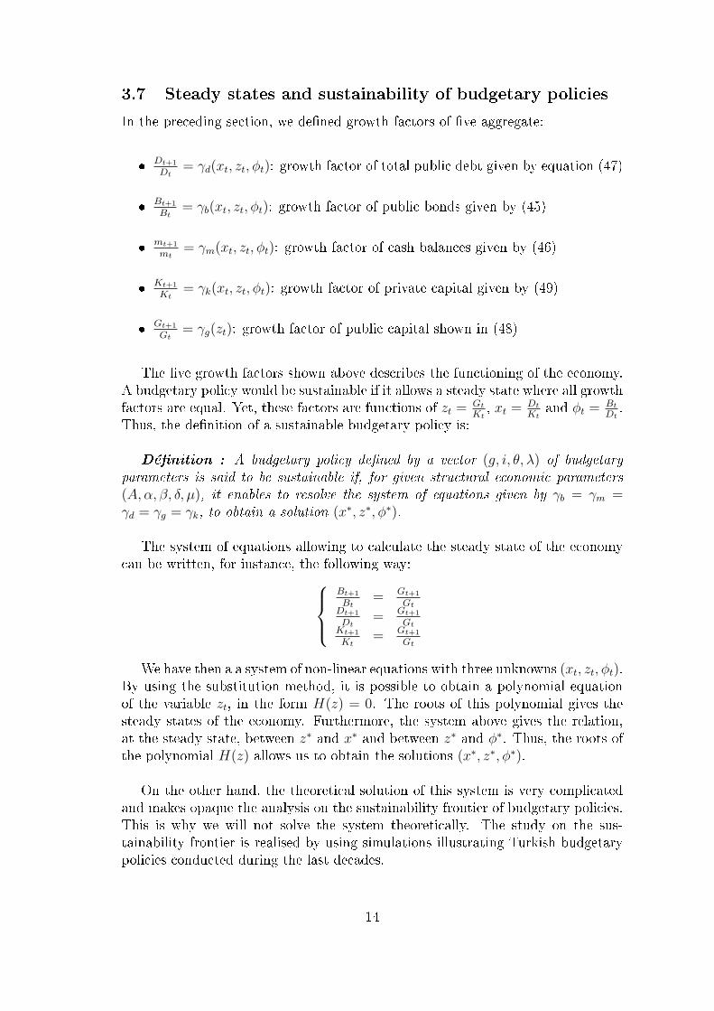
3.7 Steady states and sustainability of budgetary policies

In the preceding section, we de�ned growth factors of �ve aggregate:

�Dt+1

Dt= γd(xt, zt, φt): growth factor of total public debt given by equation (47)

�Bt+1

Bt= γb(xt, zt, φt): growth factor of public bonds given by (45)

�mt+1

mt= γm(xt, zt, φt): growth factor of cash balances given by (46)

�Kt+1

Kt= γk(xt, zt, φt): growth factor of private capital given by (49)

�Gt+1

Gt= γg(zt): growth factor of public capital shown in (48)

The �ve growth factors shown above describes the functioning of the economy.A budgetary policy would be sustainable if it allows a steady state where all growthfactors are equal. Yet, these factors are functions of zt = Gt

Kt, xt = Dt

Ktand φt = Bt

Dt.

Thus, the de�nition of a sustainable budgetary policy is:

Dé�nition : A budgetary policy de�ned by a vector (g, i, θ, λ) of budgetaryparameters is said to be sustainable if, for given structural economic parameters(A,α, β, δ, µ), it enables to resolve the system of equations given by γb = γm =γd = γg = γk, to obtain a solution (x∗, z∗, φ∗).

The system of equations allowing to calculate the steady state of the economycan be written, for instance, the following way:

Bt+1

Bt= Gt+1

GtDt+1

Dt= Gt+1

GtKt+1

Kt= Gt+1

Gt

We have then a a system of non-linear equations with three unknowns (xt, zt, φt).By using the substitution method, it is possible to obtain a polynomial equationof the variable zt, in the form H(z) = 0. The roots of this polynomial gives thesteady states of the economy. Furthermore, the system above gives the relation,at the steady state, between z∗ and x∗ and between z∗ and φ∗. Thus, the roots ofthe polynomial H(z) allows us to obtain the solutions (x∗, z∗, φ∗).

On the other hand, the theoretical solution of this system is very complicatedand makes opaque the analysis on the sustainability frontier of budgetary policies.This is why we will not solve the system theoretically. The study on the sus-tainability frontier is realised by using simulations illustrating Turkish budgetarypolicies conducted during the last decades.

14

For most of the simulations that will be presented, the polynomial H(z) has tworoots. Thus we have multiple equilibria. This is explained by increasing returnsincorporated as an externality through public capital. Only the saddle point, at-tributed to a public debt model is analysed4. In fact, the stable equilibrium givesnegative de�cits and debts.

4 SIMULATIONS - SUSTAINABILITY OF BUD-

GETARY POLICIES IN TURKEY

4.1 Methodology

As we de�ned it earlier, a budgetary policy is considered sustainable if it setsthe economy on a balanced growth path. The objective of the paper being toevaluate budgetary policies, the simulations will be focalised on steady states ofthe model. We simulate5 Turkish budgetary policies and verify if the systemγb = γd = γm = γk = γg allows a solution6 (x∗, z∗, φ∗). The existence of a so-lution implies that the simulated policy is sustainable in the long run.

Once the solution is found7, and thus the sustainability con�rmed, various longrun economic indicators can be calculated by using the stationnary values x∗, z∗

and φ∗. The long term growth rate is calculated by substituting these values inany growth factor equation, say γg. We assume that one period corresponds tothirty years8.

In�ation is calculated the same way, by substituting (x∗, z∗, φ∗) in π∗ given byequation (50). Besides in�ation and growth, we also simulate the long run valuesof public de�cit/GDP and public debt/GDP ratios, the interest rate, the weigthof cash balances, public bonds and private capital in total savings and �nally thereturn on money holdings.

First of all, we evaluate the sustainability of Turkish budgetary policies con-ducted in periods 1980-1988, 1989-1998 and 1999-2008. Then we pursue simula-tions to see the impact of budgetary parameters on sustainability and growth. Theobjective is to analyse the sustainability frontier by modifying the budget param-eters. This analysis is done within two steps.

First the 1999-2007 period is studied, during which, according to the model andsimulations, the budget policy conducted was sustainable. Taking o� from this ini-tial con�guration, we simulate alternative and more expansionnist policies. This

4See Azariadis (1993)5We use the mathematics software Maple 9.5 for simulations.6At the steady state, we assume πt+1 = πt and rt+1 = rt.7Solutions must verify the superiority of interest rate income over money holdings return.8Barro et Sala-i Martin (1995).

15

analysis enables to study the impact of each budget parameter on sustainabilityand various indicators of the economy. The results show that Turkey could haveimplemented more expansionnist and growth enhancing policies, without riskinglong run sustainability. In fact, the policy on course in this period is relativelyrestrictive and not close to the sustainability frontier.

Secondly, the policiy of period 1980-1988, which is unsustainable, is studied.We simulate alternative policies to see how sustainability could have been achieved.More precisely, the following stabilisation policies are studied : a reduction in nonproductive public spendings, a decrease in public investments, an increase in taxes,and an increase in monetization. The results show that monetization acts as a tax: it makes the budgetary policy more sustainable and creates a distorsion in port-folio choices of the agent. It triggers a fall in non-monetary savings, thus slowsdown public and private capital accumulation. Its negative impact on private cap-ital accumulation appears to be more important than that of the increase of factorincome tax.

4.2 Sustainability of Turkish budgetary policies

We analyse budgetary policies conducted in Turkey between 1980 and 2008. Wesplit this interval into three phases:

� 1980-1988 : It is the �rst liberalization period where internal public debtstarted to rise as the dominant de�cit �nancing method. Peaks of monetiza-tion are observed at the beginning and at the end of the period.

� 1989-1998 : Following the liberalization of the capital account, the economybecomes more unstable. Public debt accumulation goes on. Monetization isused at the beginning of the period while it disappears completely in 1998.

� 1999-2007 : This decade witnessed more important e�orts in macroeconomicstabilisation. Particularly in the aftermath of the crisis in 2001, successivegovernments conducted very restrictive budgetary policies recommended bythe IMF.

Structural parameters of the economy, namely (A,α, β, δ) are considered iden-tical for the three distinct periods. They are calibrated in the following way:

� Private capital elasticity9 : α = 0, 27

� Total exogenous productivity10 : A = 46

9According to estimations of Fugazza et al (2003)10Fugazza et al (2003)

16

Table 1: Sustainability of Turkish budgetary policy since 1980

Parameters 1980-1988 1989-1998 1999-2007Public spendings (g) 7,8% 10,4% 9,5%Public investments (i) 9,2% 6,3% 4,2%

Taxes (θ) 13,5% 17,1% 18,3%Share of monetization (1− λ) 24% 12% 0%

Liquidity constraint (µ) 15% 8,6% 7,4%Sustainability NO NO YES

� Intertemporal discount factor11 : β = 0, 55

� Depreciation rate of capital12 : δ = 0, 78

The parameters (g, i, θ, λ) concerning budgetary policies and the liquidity con-straint µ, di�er according to the studied period:

� The shares of current public spendings, public investments and �scal incomein the GDP (g, i, θ) are calculated using data from the overall public sectoraccounts. For the parameter θ, only �scal revenues have been taken intoaccount. All data is taken from the online databases of the State PlanningOrganization (DPT).

� The share of monetization in public de�cit �naning (1 − λ), is estimated bydividing the stock of credits granted by the Central Bank to the Treasury bythe public sector borrowing requirement of the corresponding year.

� The liquidity constraint µ is estimated by dividing the M1 monetary aggre-gate by the anual total consumption. Data on M1 aggregate are taken fromthe online database of the Central Bank of Turkey, while consumption dataare taken from the Statistical Indicators review of the Turkish Statistical In-stitute (TurkStat, 2007).

For each period mentionned, we estimate an "average" budgetary policy bysimply calculating the annual average of the budgetary parameters. Table (1)shows the calibration of each period and the result of the simulation concerningsustainability.

According to the results, budgetary policies of periods 1980-1988 and 1989-1998do not set the economy on a balanced growth path, thus are not sustainable. On

11Barro et Sala-i Martin (1995)12Barro et Sala-i Martin (1995)

17

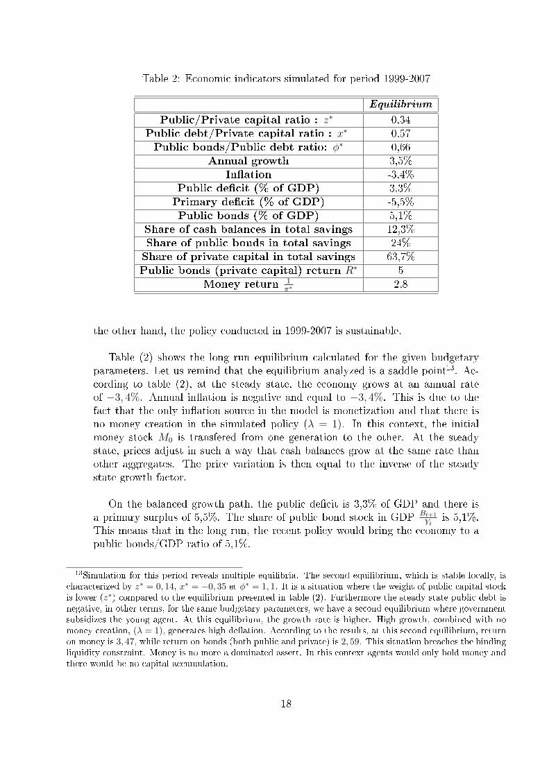
Table 2: Economic indicators simulated for period 1999-2007

Equilibrium

Public/Private capital ratio : z∗ 0,34Public debt/Private capital ratio : x∗ 0,57Public bonds/Public debt ratio: φ∗ 0,66

Annual growth 3,5%In�ation -3,4%

Public de�cit (% of GDP) 3,3%Primary de�cit (% of GDP) -5,5%Public bonds (% of GDP) 5,1%

Share of cash balances in total savings 12,3%Share of public bonds in total savings 24%Share of private capital in total savings 63,7%Public bonds (private capital) return R∗ 5

Money return 1π∗

2,8

the other hand, the policy conducted in 1999-2007 is sustainable.

Table (2) shows the long run equilibrium calculated for the given budgetaryparameters. Let us remind that the equilibrium analyzed is a saddle point13. Ac-cording to table (2), at the steady state, the economy grows at an annual rateof −3, 4%. Annual in�ation is negative and equal to −3, 4%. This is due to thefact that the only in�ation source in the model is monetization and that there isno money creation in the simulated policy (λ = 1). In this context, the initialmoney stock M0 is transfered from one generation to the other. At the steadystate, prices adjust in such a way that cash balances grow at the same rate thanother aggregates. The price variation is then equal to the inverse of the steadystate growth factor.

On the balanced growth path, the public de�cit is 3,3% of GDP and there isa primary surplus of 5,5%. The share of public bond stock in GDP Bt+1

Ytis 5,1%.

This means that in the long run, the recent policy would bring the economy to apublic bonds/GDP ratio of 5,1%.

13Simulation for this period reveals multiple equilibria. The second equilibrium, which is stable locally, ischaracterized by z∗ = 0, 14, x∗ = −0, 35 et φ∗ = 1, 1. It is a situation where the weight of public capital stockis lower (z∗) compared to the equilibrium presented in table (2). Furthermore the steady state public debt isnegative, in other terms, for the same budgetary parameters, we have a second equilibrium where governmentsubsidizes the young agent. At this equilibrium, the growth rate is higher. High growth, combined with nomoney creation, (λ = 1), generates high de�ation. According to the results, at this second equilibrium, returnon money is 3, 47, while return on bonds (both public and private) is 2, 59. This situation breaches the bindingliquidity constraint. Money is no more a dominated assett. In this context agents would only hold money andthere would be no capital accumulation.

18

According to the results, at the steady state, real cash balances (mt+1) wouldconstitute 12,3% of total savings of an agent. Public bonds (Bt+1) and privatecapital (Kt+1) would be equal to 24% and 63,6% of total savings, respectively.

4.3 The 1999-2007 period and alternative policies

Was it possible to conduct more expansionnist policies without violating the sus-tainability frontier ? If the response is positive, would the new equilibria obtainedbe better or worse than the initial one ?

In order to give a response to these questions, we conduct three series of simu-lations depicting more expansionnist budgetary policies than the initial one. First,we analyze the impact of an increase in public investments on the stability. Then,we study the e�ects of an increase in non-productive public spendings. The lastserie of simulations tests policies imposing less tax than the initial one. A �nalsimulation is realized in order to test the impact of more monetization.

The equilibrium of period 1999-2007 is a saddle point. Thus, the analysis pre-sented here is not a comparative statics. It rather aims at determining if othermore expansionnist policies could have been adopted without passing the sustain-ability frontier. It does not analyze the impact of a change in policy on the initialequilibrium.

4.3.1 Impact of public investments

Table (3) presents equilibria obtained with public investment rates (i) higher thanthat of the policy conducted in period 1999-2007. The �rst column reminds theresults of the initial policy. The others exposes alternative policies, wither higherlevels14 of (i). We see that, above i = 0, 085 approximately, the budgetary policybecomes unsustainable.

According to table (3), policies with more public investments would allow highergrowth rates. The initial growth rate of 3, 5%, with i = 0, 042, goes up to 5, 4% fora policy with i = 0, 082. Public capital is productive in the model and intervenesas an externality in private production. The marginal productivity of private cap-ital (rt = αAz1−α

t − δ) is increasing in G the public capital stock. Moreover, theincrease in R∗ shown in table (3) con�rms this impact. Increasing i moves theeconomy closer to its sustainability frontier but provides more growth enhancingequilibria.

As the growth rate becomes higher, we observe an increase in de�ation. Giventhat there is no money creation in this policy (λ=1), at the steady state return onmoney (inverse of in�ation) is equal to the long run growth rate. De�ation goes

14The initial levels of other budgetary parameters are not modi�ed

19

Table 3: Impact of an increase in public investment spendings

i=0,042 i=0,052 i=0,062 i=0,072 i=0,082

z∗ 0,34 0,39 0,43 0,46 0,45x∗ 0,57 0,51 0,4 0,3 0,1φ∗ 0,66 0,64 0,61 0,54 0,1

Annual growth 3,5% 4,1% 4,5% 5% 5,4%In�ation -3,4% -3,9% -4,3% -4,7% -5,2%

Public de�cit (% of GDP) 3,3% 3,1% 2,7% 1,9% 0,2%Primary de�cit (% of GDP) -5,5% -4,4% -3,1% -1,7% -0,1%Public bonds (% of GDP) 5,1% 4,5% 3,7% 2,5% 0,2%real cash balances/savings 12,3% 11,7% 11% 10,2% 8,9%

public bonds/savings 24% 21,2% 17,4% 11,8% 0,9%private capital/savings 63,7% 67% 71,6% 78% 90,2%Interest return R∗ 5 5,5 5,9 6,1 6Money return 1

π∗ 2,8 3,3 3,8 4,3 4,9

from 3, 4% up to 5% for i = 0, 082.

In this table, we also see that as the rate of public investments goes up, thelong run public de�cit/GDP ratio decreases. We can associate this fall to the im-portant growth rate of production. It should be noted that, paradoxally, as publicinvestments rise, public de�cit/GDP and primary de�cit/GDP get closer to 0.

One should also point the modi�cation in the composition of savings. As pub-lic investments increase, the structure of savings is modi�ed in favour of privatecapital. In fact, when i is higher, public capital stock goes up and increases themarginal productivity of private capital. Consequently, the share of private assetsin total savings rises.

4.3.2 Impact of non-productive public spendings

We now analyze the impact of an increase in non productive public spendings onsustainability. Table (4) contains the results of simulations of more expansionistbudgetary policies with higher non-productive public spendings. The �rst columngives the initial results of the 1999-2007 period budgetary policy. Above 13,4% ofpublic expenses, the other parameters being constant, the budget policy becomesunsustainable.

The in�uence of current budget expenses on sustainability and growth is similarto that of public investments. A budgetary policy containing more non-productivepublic spendings grows faster on its balanced growth path. However the e�ect ongrowth is less than that of public investments. This is due to the fact that g has

20

Table 4: Impact of an increase in non-productive public spendings

g=0,095 g=0,105 g=0,115 g=0,125

z∗ 0,34 0,32 0,29 0,26x∗ 0,57 0,5 0,37 0,24φ∗ 0,66 0,64 0,6 0,5

Annual growth 3,5% 3,57% 3,62% 3,7%In�ation -3,38% -3,4% -3,5% -3,6%

Public de�cit (% du PIB) 3,3% 2,8% 2,2% 1,3%Primary de�cit (% du PIB) -5,5% - 4,2% -2,7% -1,2%Public bonds (% du PIB) 5,1% 4,3% 3,3% 1,9%Cash balances/Savings 12,3% 11,7% 11% 10%Public bonds/Savings 24% 20,5% 16% 9%Private capital/Savings 63,7% 67,8% 73% 81%

Interest return R∗ 5 4,8 4,5 4,2Return on money 1

π∗ 2,8 2,9 2,9 3

not a direct impact on the production function. In the absence money creation,in�ation gets lower as the growth rate increases.

We also see that the more current public spendings increase the less is the publicde�cit/GDP ratio. This surprising result is also mentionned by Azariadis (1993,p.326) in an analysis of an exogenous growth model with �xed budget rules: "(...)Another process takes place at the saddle G1 in which a higher de�cit produces thecounterintuitive outcome of more capital and less public debt. The message fromthis economy is that there is no simple rule that relates the size of governmentde�cits to the steady state values of capital and debt or, for that matter, the sta-tistical correlation of physical capital and national debt. This relationship ratherstraightforward for stable steady states, is quite subtle for the saddles that are quiteoften the most economically interesting stationary equilibria."

In fact, as the budgetary policy becomes more expansionist, public de�cit/GDPand public debt/GDP ratios decrease on the saddle-point equilibrium. On the sus-tainability frontier, there is a unique equilibrium with the highest growth rate.From this point on, more expansionist budgetary policies push the economy in anunsustainable situation (no balanced growth path).

4.3.3 Impact of taxes

Simulation results for policies including less tax (θ) are presented in table (5).

As the tax rate diminishes, balanced growth rate increases, because availableincome of agents (1−θ)wt rises. Agents save more. The decrease in interest return

21

Table 5: E�ect of a decrease in tax rate

θ = 0, 183 θ = 0, 173 θ = 0, 163 θ = 0, 153

z∗ 0,34 0,31 0,29 0,26x∗ 0,57 0,48 0,37 0,25φ∗ 0,66 0,64 0,59 0,5

Annual growth 3,5% 3,57% 3,6% 3,73%In�ation -3,4% -3,44% -3,5% -3,6%

Budget de�cit (% du PIB) 3,3% 2,9% 2,3% 1,4%Primary de�cit (% du PIB) -5,5% - 4,1% -2,7% -1,33%Public bonds (% du PIB) 5,1% 4,4% 3,5% 2,2%cash balances/savings 12,3% 11,7% 11% 10%public bonds/savings 24% 20,5% 16% 10%private capital/savings 63,7% 67,7% 73% 80%Interest return R∗ 5 4,8 4,5 4,3Money return 1

π∗ 2,8 2,9 2,9 3

(R∗) also reveals a rise in non-monetary savings. Private capital is accumulatedfaster. The steady states z∗ = G

Kand x∗ = D

Kgets lower, implying an increase in

private capital K relatively to public capital G and total public debt D. However,under θ = 0, 153 the budgetary policy becomes unsustainable as there is no moresteady state solution.

4.3.4 E�ect of monetization

This paragraph analyzes the e�ect of monetization on growth and sustainability.As we did for the preceding studies, we simulate di�erent policies by decreasingprogressively the level of λ (thus increasing monetization), while we keep constantthe other budgetary parameters. The results, presented in table (6) show thatmonetization acts like a tax. As we increase monetization, we increase the in�a-tion tax, thus the new saddle-point equilibria become "more sustainable".

More monetization implies a higher money supply. In�ation is then higher asthe return on money Pt

Pt+1decreases. Due to the liquidity constraint, agents are

forced to hold more money. Thus non-monetary savings are lower. The latterbeing the source of private capital accumulation, its decrease implies a slow downin growth.

The results in table (6) con�rm this explanation. When monetization rises,steady state values of z∗ = G

Kand x∗ = D

Krise too. In other words, a larger

money supply causes a fall in the share of private capital K in the economy. Themarginal productivity of capital being decreasing, the rise in R∗ also implies thefall of private capital's relative weight.

22

Table 6: Impact d'une hausse de la monétisation

λ = 1 λ = 0, 75 λ = 0, 5 λ = 0, 25 λ = 0, 01

z∗ 0,34 0,38 0,47 0,74 7,5x∗ 0,57 0,76 1,16 2,4 30,6φ∗ 0,66 0,6 0,5 0,3 0,03

Croissance annuelle 3,5% 3,4% 3,2% 2,8% 0,98%In�ation -3,4% -2,2% -0,7% 1,3% 5%

Dé�cit budgétaire (% du PIB) 3,3% 4,5% 6,4% 9,9% 16,5%Dé�cit primaire (% du PIB) -5,5% - 5,9% -6,4% -7,4% -9,2%Titres publics (% du PIB) 5,5% 5,6% 5,2% 4,4% 0,7%encaisses réelles/épargne 12,3% 18% 29% 50% 94%titres publics/épargne 24% 25% 24,8% 21% 3%capital privé/épargne 63,7% 57% 46% 29% 3%Facteur d'intérêt R∗ 5 5,4 6,2 8,5 44,5

Rendement monnaie 1π∗ 2,8 1,9 1,2 0,7 0,24

Monetization forces the agents to hold more money in order to maintain thevalue of their real cash balances and thus slows down capital accumulation. Thispolicy also enables the �nancing of the public de�cit. Then, we observe a resourcetransfer from agents toward the government. Monetization acts as a tax. In otherwords, the rise of monetization increases the in�ation tax level and creates a sourceof income for the government. Moetization is considered then as a policy enablingsustainability.

4.4 Alternative policies for the 1980-1988 period

This last subsection studies the 1980-1988 period policy, which is unsustainable asshown in table (1). The economy in this period is situated over the sustainabilityfrontier and can not reach a balanced growth path.

We analyze possible modi�cations on the budgetary policy which would allowthe economy to reach a steady state. More precisely, we study the impacts ofan increase in monetization (decrease in λ), a decrease in non-productive publicspendings (g), a reduction in public investments (i) and �nally a rise in the taxrate (θ). For each simulation serie, we modify the level of the analyzed instrumentwhile keeping the others constant. We modify the parameters until an equilibriumis reachd, in other words until the policy becomes sustainable.

23

4.4.1 Monetization as a stabilization instrument

Let us �rst remind the Turkish budgetary parameters of period 1980-1988 whichis unable to reach a balanced growth path:

� Share of public de�cit �nanced by bond issuance : λ = 0, 76

� Share of public investments in GDP : i = 0, 092

� Share of current public expenditures in GDP : g = 0, 078

� Tax rate : θ = 0, 135

We simulate alternative policies by reducing λ, in other words by increasingmonetization. The policy becomes sustainable from λ = 0, 18 on. This means that�nancing 82% of public de�cit by creating money would have allowed the economyto reach a balanced growth path. Table (7), presented in appendix, shows thedetails of the saddle point equilibrium obtained with this new policy.

The growth rate recorded at this new equilibrium (5, 1%) is much higher thanthe rate obtained with the policy of period 1999-2007 (3, 46%). This di�erence isdue to the high level of public investments in period 1980-1988.

4.4.2 Other methods of stabilization

In addition to the increase of monetization, three other stabilization policies aresimulated. According to the results:

� Sustainability is obtained if non-productive public spendings/GDP falls fromg = 0, 078 to g = 0, 039. Details of the equilibrium obtained are presented intable (8) in appendix.

� A reduction of public investment/GDP ratio from i = 0, 092 to i = 0, 052stabilizes the economy. Table (9) in appendix presents the details of the newequilibrium.

� A rise in taxes from θ = 0, 135 to θ = 0, 175 makes the budgetary policy sus-tainable. The details of the equilibrium are shown in table (10) in appendix.

Comparing tables (7), (8), (9) and (10), we see that the stabilization methodallowing maximum growth rate is the decrease in non-productive public spendings(5, 7%). The rise in taxes allows a stable growth rate of 5,6%. On the other hand,the most unfavourable method in growth terms appears to be the decrease of publicinvestments 4, 3%), due to the important in�uence of this variable in productivity.

24

It is interesting to compare the impact of tax increase and monetization in thestabilization of the economy. The balanced growth path obtained by raising taxeson factor income (θ) allows a higher growth rate (5, 6%) than the one obtained byraising in�ation tax (5, 1%).

It is then possible to correct an unsustainable budgetary policy by increasingmonetization and thus by collecting an in�ation tax. On the other hand, withgiven structural and budgetary parameters, reaching sustainability through a risein factor income taxes is more advantageous. The most advantageous stabilizationmethod, according to our results, is a reduction of non-productive public spend-ings. Finally, the most unfavourable method is a fall in public investments.

5 CONCLUDING REMARKS

This paper presented an endogenous growth model with OLG settings where pro-ductive public capital is incorporated as an externality and money is includedthrough a liquidity constraint. The government, in the model, realizes productiveand unproductive spendings whose amounts are expressed as a share of GDP. Italso �xes a tax rate on factor income and determines the share of bond issuanceand monetization in public de�cit �nancing. The latter is exogenous in our model,while the other budgetary parameters are constant and allows to �x budget rules.A �xed budget policy allowing the economy to reach a balanced growth path isconsidered as sustainable.

This theoretical framework enables to analyze the sustainability of Turkish bud-getary policies between 1980 and 2007. Our simulation results show that policiesconducted in 1980-1988 and 1989-1998 periods are unsustainable, while the "av-erage" policy applied in period 1999-2007 is sustainable. Further simulations onalternative policies showed that more expansionist policies could have been con-ducted in 1999-2007 period without breaching sustainability.

The model also illustrates the tax in�ation mechanism. Simulations show howmonetization acts as a tax. It enables sustainability but creates in�ation and slowsdown private capital accumulation through a fall in non-monetary savings. Thelatter is due to the liquidity constraint which forces agents to hold more moneywhen money supply and in�ation rise. Although monetization cen be consideredas a tax, its negative e�ect on private capital accumulation is greater than thatof factor income taxes. Thus, according to the model, increasing taxes is a bet-ter policy than increasing monetization in order to reach a balanced growth path.However, increasing taxes in a less developed or developed country is not as easieras it is in a developed country.

25

6 APPENDIX

6.1 Dynamic of cash balances

We have the equality :

mt+1

mt

− 1

πt= (1− λ)(g + i− θ) Yt

mt

+ (1− λ)(1− θ)rtBt

mt

+ (1− λ)θδKt

mt

The ratio Ytmt

can be re-written the following way:

Ytmt

=YtKt

Kt

Dt

Dt

mt

Ytmt

=YtKt

1

xt(1− φt)

We know YtKt

from the relation (41), and rt from (44). Introducing these termswe express the growth of cash balances as:

mt+1

mt

= (1− λ)(g + i− θ) Az1−αt

xt(1− φt)+ (1− λ)(1− θ)

(φt

1− φt

)(αAz1−α

t − δ)

+(1− λ)θδ

xt(1− φt)+

1

πt

6.2 Growth of total public debt

Our starting point is the accumulation dynamic given by (28) :

Dt+1 −Dt = (g + i− θ)Yt + (1− θ)Bt + θδKt −mt

(1− 1

πt

)We divide this equation by Dt :

Dt+1

Dt

= (g + i− θ) YtDt

+ (1− θ)rtBt

Dt

+θδKt

Dt

+

(1− 1

πt

)mt

Dt

+ 1

Yet we already know the following :

YtDt

=YtKt

Kt

Dt

=Az1−α

t

xtBt

Dt

= φt

Kt

Dt

=1

xtrt = αAz1−α

t − δmt

Dt

= 1− φt

26

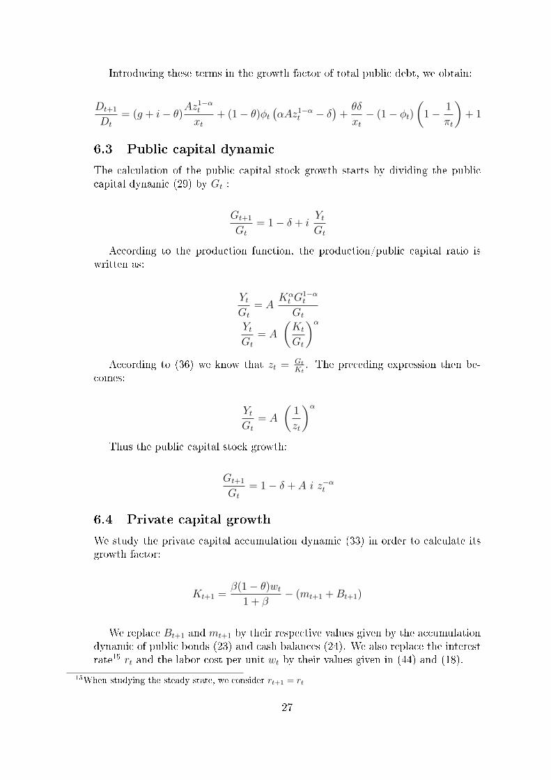
Introducing these terms in the growth factor of total public debt, we obtain:

Dt+1

Dt

= (g + i− θ)Az1−αt

xt+ (1− θ)φt

(αAz1−α

t − δ)

+θδ

xt− (1− φt)

(1− 1

πt

)+ 1

6.3 Public capital dynamic

The calculation of the public capital stock growth starts by dividing the publiccapital dynamic (29) by Gt :

Gt+1

Gt

= 1− δ + iYtGt

According to the production function, the production/public capital ratio iswritten as:

YtGt

= AKαt G

1−αt

Gt

YtGt

= A

(Kt

Gt

)αAccording to (36) we know that zt = Gt

Kt. The preceding expression then be-

comes:

YtGt

= A

(1

zt

)αThus the public capital stock growth:

Gt+1

Gt

= 1− δ + A i z−αt

6.4 Private capital growth

We study the private capital accumulation dynamic (33) in order to calculate itsgrowth factor:

Kt+1 =β(1− θ)wt

1 + β− (mt+1 +Bt+1)

We replace Bt+1 and mt+1 by their respective values given by the accumulationdynamic of public bonds (23) and cash balances (24). We also replace the interestrate15 rt and the labor cost per unit wt by their values given in (44) and (18).

15When studying the steady state, we consider rt+1 = rt

27

Kt+1 =β(1− θ)(1− α)

1 + βYt − (g + i− θ)Yt − θδKt − (1− θ)Btrt −Bt −

mt

πt

Then we divide this expression by Kt. During this operation, we realize thefollowing transformations: Yt

Kt= Az1−α

t , BtKt

= BtDt

DtKt

= φtxt and rt =(αAz1−α

t − δ).

We obtain :

Kt+1

Kt=β(1− θ)(1− α)

1 + βAz1−α

t − (g + i− θ)Az1−α − θδ −(1 + (1− θ)(αAz1−α

t − δ))φtxt −

(1− φt)xtπt

6.5 In�ation

The cash-in-advance constraint requires:

µPt+1cv,t+1 = Mt+1

Dividing both sides by Pt and introducing variables mt+1 = Mt+1

Ptand πt+1 =

Pt+1

Ptwe get :

πt+1 =mt+1

µcv,t+1

In this expression, we replace cv,t+1 by its value given by the intertemporalmaximizing program of the agent shown in(13) :

πt+1 =mt+1(1 + β)(1− µ+ µπt+1Rt+1)

µβ(1− θ)wtRt+1

Replace labor cost wt by its marginal productivity with (18) :

πt+1 =mt+1(1 + β)(1− µ+ µπt+1Rt+1)

µβ(1− θ)(1− α)YtRt+1

(51)

Divide both the numerator and the denominator of the fraction situated on theright side by mt+1. We then have to express Yt

mt+1in terms of xt, zt et φt:

Ytmt+1

=Ytmt

mt

mt+1

(52)

The part Ytmt

can easily be written in terms of xt, zt and φt :

28

Ytmt

=YtDt

Dt

mt

=YtKt

Kt

Dt

1

1− φt

=Az1−α

t

xt(1− φt)

We denote the growth factor of cash balances shown in (52) as γm = mt+1

mt.

Incorporating (52) in (51) and developing Rt+1 according to (4) we determine theprice dynamic:

πt+1 =(1 + β)(1− µ)

µ(1 + (1− θ)(αAz1−αt − δ))

(β(1−θ)(1−α)Az1−αt

xt(1−φt)γm − 1− β) (53)

29

6.6 Results of Simulations of Stabilization Policies

Table 7: Sustainability obtained by monetization

Steady state value

public capital/private capital : z∗ 1public debt/private capital : x∗ 1,4

Public bonds/total public debt: φ∗ 0,1Annual growth 5,1%

In�ation -2,2%Public de�cit (% of GDP) 7,6%Primary de�cit (% of GDP) 3,1%Public bonds (% du PIB) 1,7%cash balances/savings 50,2%public bonds/savings 7,4%private capital/savings 42,4%

return on public bonds R∗ 11,2return on money 1

π∗2

30

Table 8: Sustainability reached by reducing non-productive public spendings

Steady state value

public capital/private capital : z∗ 0,54public debt/private capital : x∗ 0,27public bonds/public debt: φ∗ 0,07

Annual growth 5,7%In�ation -5,3%

public de�cit (% of GDP) 0,35%primary de�cit (% of GDP) -0,1%public bonds (% of GDP) 0,3%cash balances/savings 20%public bonds/savings 1,5%private capital/savings 78,5%return on bonds R∗ 7,2return on money 1

π∗5

Table 9: Sustainability attained through public investments reduction

Steady state value

public capital/private capital: z∗ 0,3public debt/private capital: x∗ 0,2public bonds/public debt: φ∗ -0,1

Annual growth 4,3%In�ation -4,2%

public de�cit (% of GDP) -0,5%primary de�cit (% of GDP) 0,1%public bonds (% of GDP) -0,1%cash balance/savings 18,7%public bonds/savings -2,2%private capital/savings 83,5%

bonds return R∗ 4,7money return 1

π∗3,6

31

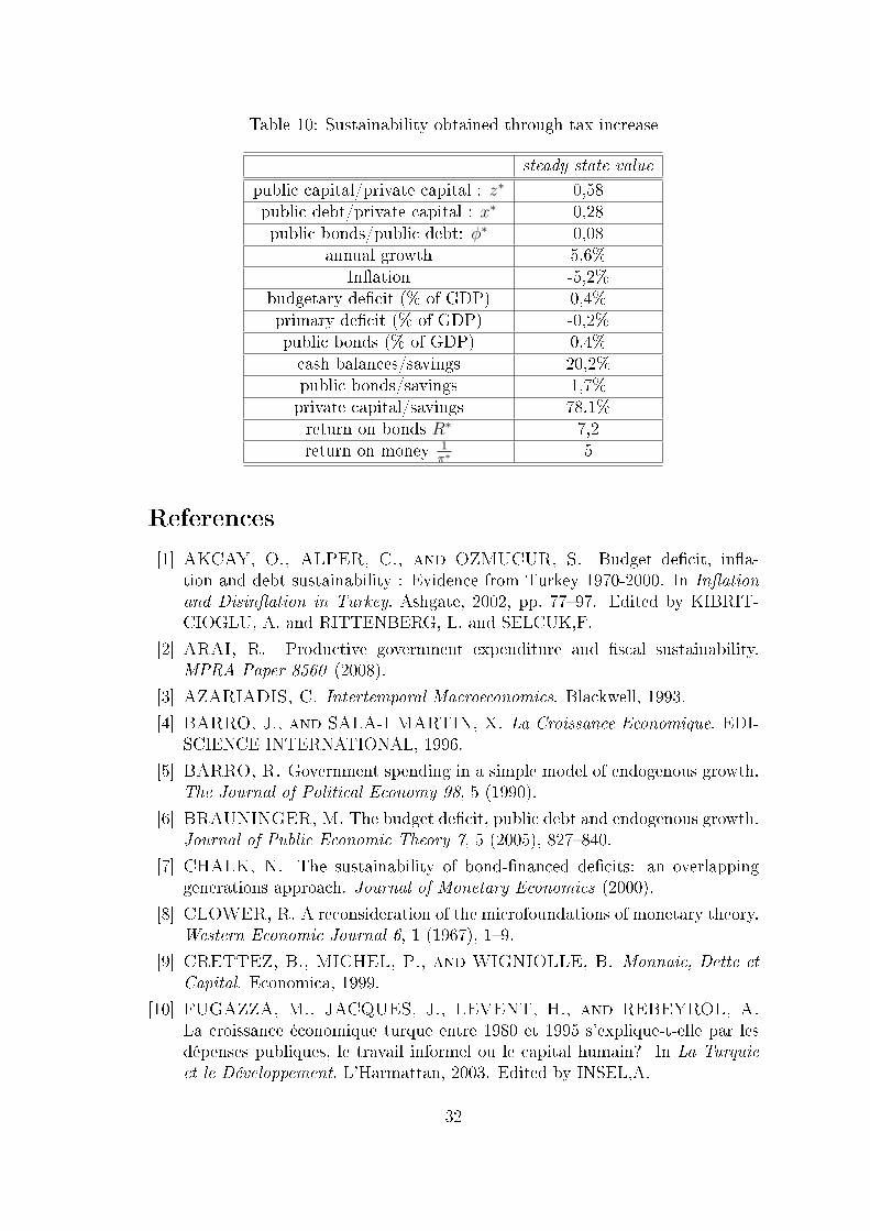
Table 10: Sustainability obtained through tax increase

steady state value

public capital/private capital : z∗ 0,58public debt/private capital : x∗ 0,28public bonds/public debt: φ∗ 0,08

annual growth 5,6%In�ation -5,2%

budgetary de�cit (% of GDP) 0,4%primary de�cit (% of GDP) -0,2%public bonds (% of GDP) 0,4%cash balances/savings 20,2%public bonds/savings 1,7%private capital/savings 78,1%return on bonds R∗ 7,2return on money 1

π∗5

References

[1] AKCAY, O., ALPER, C., and OZMUCUR, S. Budget de�cit, in�a-tion and debt sustainability : Evidence from Turkey 1970-2000. In In�ationand Disin�ation in Turkey. Ashgate, 2002, pp. 77�97. Edited by KIBRIT-CIOGLU, A. and RITTENBERG, L. and SELCUK,F.

[2] ARAI, R. Productive government expenditure and �scal sustainability.MPRA Paper 8560 (2008).

[3] AZARIADIS, C. Intertemporal Macroeconomics. Blackwell, 1993.

[4] BARRO, J., and SALA-I MARTIN, X. La Croissance Economique. EDI-SCIENCE INTERNATIONAL, 1996.

[5] BARRO, R. Government spending in a simple model of endogenous growth.The Journal of Political Economy 98, 5 (1990).

[6] BRAUNINGER, M. The budget de�cit, public debt and endogenous growth.Journal of Public Economic Theory 7, 5 (2005), 827�840.

[7] CHALK, N. The sustainability of bond-�nanced de�cits: an overlappinggenerations approach. Journal of Monetary Economics (2000).

[8] CLOWER, R. A reconsideration of the microfoundations of monetary theory.Western Economic Journal 6, 1 (1967), 1�9.

[9] CRETTEZ, B., MICHEL, P., and WIGNIOLLE, B. Monnaie, Dette etCapital. Economica, 1999.

[10] FUGAZZA, M., JACQUES, J., LEVENT, H., and REBEYROL, A.

La croissance économique turque entre 1980 et 1995 s'explique-t-elle par lesdépenses publiques, le travail informel ou le capital humain? In La Turquieet le Développement. L'Harmattan, 2003. Edited by INSEL,A.

32

[11] FUTAGAMI, K., MORITA, Y., and SHIBATA, A. Dynamic analysis ofan endogenous growth model with public capital. Scandinavian Journal ofEconomics 95 (4) (1993), 607�625.

[12] FUTAGAMI, K., and SHIBATA, A. Budget de�cits and economic growth.Discussing Paper, Center for Intergenerational Studies, Institute of EconomicResearch, Hitotsubashi University 133 (2003).

[13] GURBUZ, Y., JOBERT, T., and TUNCER, R. Public debt in Turkey :evaluation and perspectives. Applied Economics 39 (2007), 343�359.

[14] HAHN, F., and SOLOW, R. A critical essay on modern macroeconomictheory. Basil Backwell, 1995.

[15] LUCAS, R., and STOCKEY, N. Money and interest rate in a cash-in-advance economy. Econometrica 55, 3 (1987), 491�513.

[16] MEROLA, R. Fiscal sustainability in Turkey during 1970-2002. Universityof Rome 'Tor Vergata' (2006).

[17] RANKIN, N., and ROFFIA, B. Maximum sustainable government debt inoverlapping generations model. Manchester School 71, 3 (2003), 217�241.

[18] VILLIEU, P. Contrainte de disposition préalable de monnaie et déséquilibresmacroéconomiques. PhD thesis, Université Paris-I, 1992.

[19] VOYVODA, E., and YELDAN, E. Managing Turkish debt : An OLGinvestigation of the IMF's �scal programming model for Turkey. Journal ofPolicy Modeling 27, 6 (2005), 743�765.

[20] YAKITA, A. Sustainability of public debt, public capital formation, andendogenous growth in an overlapping setting. Journal of Public Economics92 (2008), 897�914.

[21] CENTRAL BANK OF TURKEY, Web site - Database.http://www.tcmb.gov.tr.

[22] STATE PLANNING ORGANIZATION, Web site - Database - Public ac-counts. http://www.dpt.gov.tr.

[23] TURKSTAT - Turkish Statistical Intitute, web site.http://www.turkstat.gov.tr/Start.do.

33