pseudo-marginal hamiltonian monte carlo
TRANSCRIPT
Journal of Machine Learning Research 22 (2021) 1-45 Submitted 6/19; Revised 5/21; Published 6/21
Pseudo-Marginal Hamiltonian Monte Carlo
Johan Alenlov [email protected] of Statistics and Machine LearningLinkoping UniversityLinkoping, 581 83, Sweden
Arnaud Doucet [email protected] of StatisticsUniversity of OxfordOxford, OX1 3TG, United Kingdom
Fredrik Lindsten [email protected] of Statistics and Machine LearningLinkoping UniversityLinkoping, 581 83, Sweden
Editor: Ryan Adams
AbstractBayesian inference in the presence of an intractable likelihood function is computationallychallenging. When following a Markov chain Monte Carlo (MCMC) approach to approxi-mate the posterior distribution in this context, one typically either uses MCMC schemeswhich target the joint posterior of the parameters and some auxiliary latent variables, orpseudo-marginal Metropolis—Hastings (MH) schemes. The latter mimic a MH algorithmtargeting the marginal posterior of the parameters by approximating unbiasedly the in-tractable likelihood. However, in scenarios where the parameters and auxiliary variables arestrongly correlated under the posterior and/or this posterior is multimodal, Gibbs samplingor Hamiltonian Monte Carlo (HMC) will perform poorly and the pseudo-marginal MHalgorithm, as any other MH scheme, will be inefficient for high-dimensional parameters. Wepropose here an original MCMC algorithm, termed pseudo-marginal HMC, which combinesthe advantages of both HMC and pseudo-marginal schemes. Specifically, the PM-HMCmethod is controlled by a precision parameter N , controlling the approximation of thelikelihood and, for any N , it samples the marginal posterior of the parameters. Additionally,as N tends to infinity, its sample trajectories and acceptance probability converge to thoseof an ideal, but intractable, HMC algorithm which would have access to the intractablelikelihood and its gradient. We demonstrate through experiments that PM-HMC canoutperform significantly both standard HMC and pseudo-marginal MH schemes.Keywords: Hamiltonian Monte Carlo, pseudo-marginal, Markov chain Monte Carlo,latent variable models
1. Introduction
Let y ∈ Y denote some observed data and θ ∈ Θ ⊆ Rd denote parameters of interest. Wewrite θ 7→ p(y | θ) for the likelihood of the observations and we assign a prior for θ of densityp(θ) with respect to Lebesgue measure dθ. Hence the posterior density of interest is given
c©2021 Johan Alenlov, Arnaud Doucet and Fredrik Lindsten.
License: CC-BY 4.0, see https://creativecommons.org/licenses/by/4.0/. Attribution requirements are providedat http://jmlr.org/papers/v22/19-486.html.
Alenlov, Doucet and Lindsten
byπ(θ) = p(θ | y) ∝ p(y | θ)p(θ). (1)
For complex Bayesian models, the posterior (1) needs to be approximated numerically.When the likelihood p(y | θ) can be evaluated pointwise, this can be achieved using standardMCMC schemes. However, we will consider here the scenario where p(y | θ) is intractable, inthe sense that it cannot be evaluated pointwise. We detail below two important scenarioswhere an intractable likelihood occurs.Example: Latent variable models. Consider the model
Xki.i.d.∼ fθ(·), Yk |Xk ∼ gθ(· |Xk), (2)
where (Xk)k≥1 are Rn-valued latent variables, (Yk)k≥1 are Y-valued. We write i : j :=i, i+ 1, ..., j for any i ≤ j. Having observed Y1:T = y1:T = y (thus, Y = YT ) the likelihoodis given by p(y1:T | θ) =
∏Tk=1 p(yk | θ), where each term p(yk | θ) satisfies
p(yk | θ) =∫Rn
fθ(xk)gθ(yk |xk)dxk. (3)
If the integral (3) cannot be computed in closed form then the likelihood p(y1:T | θ) isintractable.Example: Approximate Bayesian computation (ABC). Consider the scenario whereθ 7→ p(y | θ) is the “true” likelihood function. We cannot compute it pointwise but we assumewe are able to simulate some pseudo-observations Z ∼ p(· | θ) using Z = γ(θ, V ) whereV ∼ λ(·) for some auxiliary variable distribution λ and mapping γ : Θ× V → Y. Given akernel K : Y × Y →R+, the ABC approximation of the posterior is given by (1) where theintractable ABC likelihood is
p(y | θ) =∫YK(y | z)p(z | θ)dz =
∫K(y | γ(θ, v))λ(v)dv. (4)
Two standard approaches to perform MCMC in these scenarios are:
1. Implement standard MCMC algorithms to sample from the joint distribution of theparameters and auxiliary variables; e.g. in the latent variable context we would tar-get p(θ, x1:T | y1:T ) ∝ p(θ)
∏Tk=1 fθ(xk)gθ(yk |xk) and in the ABC context p(θ, v | y) ∝
p(θ)λ(v)K(y | γ(θ, v)). Gibbs-type approaches alternate between sampling from the pa-rameters conditioned on the data and auxiliary variables, and sampling the auxiliaryvariables conditioned on the parameters and data. These approaches can converge veryslowly if these variables are strongly correlated under the target (Andrieu et al., 2010,Section 2.3). Hamiltonian Monte Carlo (HMC) methods (Duane et al., 1987) offer a possi-ble remedy, but can also struggle in cases where there are strong non-linear dependenciesbetween variables, or when the joint posterior is multimodal (Neal, 2011, Section 5.5.7).
2. Use a pseudo-marginal MH algorithm jointly accepting or rejecting the parameters andauxiliary variables replacing the intractable likelihood term by a non-negative unbiasedestimate of the true likelihood; see (Andrieu et al., 2010; Andrieu and Roberts, 2009;
2

Pseudo-Marginal Hamiltonian Monte Carlo
Beaumont, 2003; Flury and Shephard, 2011; Lin et al., 2000). For example, in the ABCcontext the pseudo-marginal MH algorithm is a MH algorithm targeting p(θ, v | y) using aproposal distribution q(θ, θ′)λ(v′). As for any MH algorithm, it can be difficult to select aproposal q(θ, θ′) which results in an efficient sampler when Θ is high-dimensional.
In many scenarios, the marginal posterior (1) will have a “nicer” structure than the jointposterior of the parameters and auxiliary variables which often exhibit complex patterns ofdependence and multimodality. For example, discrete choice models are a widely popularclass of models in health economics, e-commerce, marketing and social sciences used toanalyze choices made by consumers, individuals or businesses (Train, 2009). When thepopulation is heterogeneous, such models can be represented as (2) where fθ(·) is a mixturedistribution, the number of components representing the number of latent classes; see e.g.(Burda et al., 2008). In this context, the paucity of data typically available for each individualis such that the joint posterior p(θ, x1:T | y1:T ) = p(θ | y1:T )
∏Tk=1p(xk | yk, θ) will be highly
multimodal while the marginal p(θ | y1:T ) will only have symmetric well-separated modesfor T large enough (or one mode if constraints on the mixture parameters are introduced).Such problems also arise in biostatistics (Komarek and Lesaffre, 2008). In these scenarios,current MCMC methods will be inefficient. In this article, we propose a novel HMC scheme,termed pseudo-marginal HMC (PM-HMC), which mimics the HMC algorithm targeting themarginal posterior (1) while integrating out numerically the auxiliary variables. The methodis a so called exact approximation in the sense that its limiting distribution (marginally in θ)is exactly π(θ), despite the fact that the algorithm is using a finite-precision approximationof the likelihood internally.
1.1 Related Work
Stochastic gradient MCMC (Welling and Teh, 2011; Chen et al., 2014; Ding et al., 2014;Leimkuhler and Shang, 2016)—including HMC-like methods—are a popular class of algo-rithms for approximate posterior sampling when an unbiased estimate of the log-likelihoodgradient is available. The typical scenario is when the number of data points T is prohibitivelylarge for evaluating the full gradient, in which case subsampling (mini-batching) can be usedto approximate the gradient unbiasedly. This is in contrast with the setting studied in thispaper, where we assume that we have access to an unbiased estimate of the likelihood itself,but not of the log-likelihood gradient. Furthermore, these methods are inconsistent for finitestep sizes and typically require some type of variance reduction techniques to be efficient(Shang et al., 2015). Recently, Umenberger et al. (2019) have proposed to use debiasing(Jacob et al., 2020) of log-likelihood gradients within stochastic gradient HMC, but thisstill results in an inconsistent method. Another approach to solving this issue is by Danget al. (2019), who proposes the use of energy-conserving subsampling which combined witha signed pseudo-marginal algorithm (Quiroz et al., 2021) can be made exact.
Hamiltonian ABC (Meeds et al., 2015) also performs HMC with stochastic gradientsbut calculates these gradients by using forward simulation. Similarly to stochastic gradientMCMC (and in contrast with PM-HMC), this results in an approximate MCMC which doesnot preserve the distribution of interest. Constrained HMC (Graham and Storkey, 2017)uses HMC to jointly infer the parameters and auxiliary variables in an auxiliary variableformulation of a Gaussian kernel ABC posterior.
3
Alenlov, Doucet and Lindsten
Kernel HMC (Strathmann et al., 2015) is another related approach which approximatesthe gradients by fitting an exponential family model in a reproducing kernel Hilbert space.If the adaptation of the kernel stops after a finite time, or if the adaptation probabilitydecays to zero, then the method can be shown to attain detailed balance, and thus targetsthe correct distribution of interest. However, the kernel-based approximation gives riseto a bias in the gradients which is difficult to control and there is no guarantee that thetrajectories closely follow the ideal HMC. Kernel HMC requires the selection of a kerneland, furthermore, some appropriate approximation thereof, since the computational cost ofa full kernel-based approximation grows cubically with the number of MCMC iterations; seeStrathmann et al. (2015) for details.
Pseudo-marginal slice sampling (Murray and Graham, 2016) is closely related to PM-HMC in the sense that both algorithms target the same extended distribution (given by (8)in the next section) as the pseudo-marginal MH and are therefore also exact approximations(Andrieu and Roberts, 2009). Pseudo-marginal slice sampling relies instead on alternatingthe sampling of the parameters given the likelihood estimate and sampling the likelihoodestimate given the parameters. In this framework different MCMC methods such as slicesampling (Neal, 2003) and Metropolis—Hastings can be used to sample from the conditionaldistributions—typically one always uses elliptical slice sampling (Murray et al., 2010) forsampling of the likelihood estimates. In comparison our proposed algorithm samples jointlythe parameters and the likelihood estimate.
Building on a preprint of the present article Nemeth et al. (2019) have proposed the socalled pseudo-extended HMC method for sampling multimodal target distributions. Thiscan be viewed as a special case of PM-HMC applied to a model with a single latent variableand no top-level parameter. Osmundsen et al. (2018) have also built on the present workand propose a version of PM-HMC using efficient importance sampling, which they apply toinference in dynamical systems.
1.2 Outline of the Paper
Our paper is organized as follows. In Section 2 we present our algorithm by first introducing inSection 2.1 the standard HMC method. The PM-HMC algorithm is presented in Section 2.2with an illustration on the latent variable model in Section 2.3. In Section 2.4 we presenta customized numerical integrator—an essential component of PM-HMC that is neededfor handling the increasing dimension of the latent variable space. This completes thespecification of the PM-HMC algorithm. The theoretical justification of our algorithmis presented in Section 3 with the proofs postponed to the appendix. Finally we presentnumerical results demonstrating the usefulness of our algorithm in Section 4.
2. Pseudo-marginal Hamiltonian Monte Carlo
In this section we present the proposed method. First we give some background on Hamilto-nian Monte Carlo (HMC) and, specifically, we consider the case of targeting the marginalposterior π(θ) using HMC. This results in an ideal but intractable algorithm. We thenpresent PM-HMC, an exact approximation of the marginal HMC.
4

Pseudo-Marginal Hamiltonian Monte Carlo
2.1 Marginal Hamiltonian Monte Carlo
The Hamiltonian formulation of classical mechanics is at the core of HMC methods. Recallthat θ ∈ Θ ⊆ Rd. We identify the potential energy as the negative unnormalized log-targetand introduce a momentum variable ρ ∈ Rd which defines the kinetic energy 1
2ρ>ρ of the
system.1 The resulting “exact” Hamiltonian is given by
Hex(θ, ρ) = − log p(θ)− log p(y | θ) + 12ρ>ρ. (5)
We associate a probability density on Rd × Rd to this Hamiltonian through
π(θ, ρ) ∝ exp(−Hex(θ, ρ)) = π(θ)N (ρ | 0d, Id), (6)
where N (z |µ,Σ) denotes the normal density of argument z, mean µ and covariance Σ.Assuming that the prior density and likelihood function are continuously differentiable,
the Hamiltonian dynamics corresponds to the equations of motion
dθdt = ∇ρHex = ρ,
dρdt = −∇θHex = ∇θ log p(θ) +∇θ log p(y | θ). (7)
A key property of this dynamics is that it preserves the Hamiltonian, i.e. Hex(θ(t), ρ(t)) =Hex(θ(0), ρ(0)) = H0 for any t ≥ 0. This enables large moves in the parameter space to bemade by simulating the Hamiltonian dynamics. However, to sample from the posterior, it isnecessary to explore other level sets of the Hamiltonian; this can be achieved by periodicallyupdating the momentum ρ according to its marginal under π, i.e. ρ ∼ N (0d, Id).
The Hamiltonian dynamics only admits a closed-form solution in very simple scenarios,e.g., if π(θ) is normal. Hence, in practice, one usually needs to resort to a numericalintegrator. Typically, the Verlet method, also known as the Leapfrog method, is used due toits favourable properties in the context of HMC (Leimkuhler and Matthews, 2015, p. 60;Neal, 2011, Section 5.2.3.3). In particular, this integrator is symplectic which implies that theJacobian of the transformation (θ(0), ρ(0))→ (θ(t), ρ(t)) is unity for any t > 0. Because ofnumerical integration errors, the Hamiltonian is not preserved along the discretized trajectorybut this can be accounted for by an MH rejection step. The resulting HMC method is givenby the following: at state θ := θ[0], (i) sample the momentum variable ρ[0] ∼ N (0d, Id),(ii) simulate approximately the Hamiltonian dynamics over L discrete time steps usinga symplectic integrator, yielding (θ[L], ρ[L]), and (iii) accept (θ[L], ρ[L]) with probability1 ∧ π(θ[L], ρ[L])/π(θ[0], ρ[0]) = 1 ∧ exp(Hex(θ[0], ρ[0])−Hex(θ[L], ρ[L])). We refer to Neal(2011) for details and a more comprehensive introduction.
2.2 Pseudo-Marginal Hamiltonian dynamics
When the likelihood is intractable, it is not possible to approximate numerically the Hamil-tonian dynamics (7), as the integrator requires evaluating ∇θ log p(y | θ) pointwise. We willaddress this difficult by instead considering a Hamiltonian system defined on an extendedphase space when the following assumption holds.
1. For simplicity we assume unit mass. The extension to a general mass matrix is straightforward.
5

Alenlov, Doucet and Lindsten
• Assumption 1. There exists (θ,u) 7→ p(y | θ,u) ∈ R+ where u ∈ U and m(·) a probabilitydensity on U such that p(y | θ) =
∫p(y | θ,u)m(u)du.
Assumption 1 equivalently states that p(y | θ,U) is a non-negative unbiased estimate ofp(y | θ) when U ∼ m(·). This assumption is at the core of pseudo-marginal methods (Andrieuand Roberts, 2009; Deligiannidis et al., 2018; Lin et al., 2000; Murray and Graham, 2016)which rely on the introduction of an extended target density
π(θ,u) = π(θ) p(y | θ,u)p(y | θ) m(u) ∝ p(θ)p(y | θ,u)m(u). (8)
This extended target admits π(θ) as a marginal under Assumption 1. The pseudo-marginalMH algorithm is for example a ‘standard’ MH algorithm targeting (8) using the proposalq(θ, θ′)m(u′) when in state (θ,u), resulting in an acceptance probability
1 ∧ p(θ′)p(y | θ′,u′)
p(θ)p(y | θ,u)q(θ′, θ)q(θ, θ′) . (9)
Instead of exploring the extended target distribution π(θ,u) using an MH strategy, we willrely here on an HMC mechanism. Our method will use an additional assumption on thedistribution of the auxiliary variables and regularity conditions on the simulated likelihoodfunction p(y | θ,u).
• Assumption 2. U =RD, m(u) = N (u | 0D, ID), (θ,u) 7−→ p(y | θ,u) is continuouslydifferentiable and (θ,u) 7−→ ∇(θ,u) log p(y | θ,u) can be evaluated point-wise.
Our algorithm will leverage the fact that m(u) is a normal distribution. Assumptions 1 and 2will be standing assumptions from now on and allow us to define the following extendedHamiltonian
H(θ, ρ,u,p) = − log p(θ)− log p(y | θ,u) + 12ρTρ+ uTu + pTp
, (10)
with a corresponding joint probability density on R2d+2D
π(θ, ρ,u,p) = π(θ,u)N (ρ | 0d, Id)N (p | 0D, ID) ∝ exp(−H(θ, ρ,u,p)), (11)
which also admits π(θ) as a marginal. Here p ∈ RD are momentum variables associatedwith u. The corresponding equations of motion associated with this extended Hamiltonianare then given by
ddt
θρup
=
ρ
∇θ log p(θ) +∇θ log p(y | θ,u)p
−u +∇u log p(y | θ,u)
:= Ψ(θ, ρ,u,p). (12)
Compared to (7), the intractable log-likelihood gradient ∇θ log p(y | θ) appearing in(7) has now been replaced by the gradient ∇θ log p(y | θ,u) of the log-simulated likelihoodp(y | θ,u) where u evolves according to the third and fourth rows of (12).
6
Pseudo-Marginal Hamiltonian Monte Carlo
Remark 1 The normality assumption is in itself not restrictive as we can think of u as theinternal random variables used to compute the likelihood estimator (we can always generate,e.g., a uniform random variate from a normal one using the cumulative distribution function).This assumption has also been used by Deligiannidis et al. (2018) for the correlated pseudo-marginal MH method and Murray and Graham (2016) for pseudo-marginal slice sampling.However, the assumed regularity of the simulated likelihood function p(y | θ,u) limits its rangeof applications. For example, in a state-space model context the likelihood is usually estimatedusing a particle filter, as in Andrieu et al. (2010), but this results in a discontinuous function(θ,u) 7−→ p(y | θ,u).
In latent variable models the use of the auxiliary variables will be to construct animportance sampling estimator. In such cases, the user has the freedom to specify theimportance distribution such that Assumption 2 is satisfied. In particular, it can be differfrom the prior distribution of the latent variables. We use this freedom in the numericalexample in Section 4.3.
2.3 Illustration on Latent Variable Models
Consider the latent variable model described by (2) and (3). In this scenario, the intractablelikelihood can be unbiasedly estimated using importance sampling. We introduce animportance density qθ(xk | yk) for the latent variable Xk which we assume can be simulatedusing Xk = γk(θ, V ) where γk : Θ×Rp → Rn is a deterministic map and V ∼ N (0p, Ip). Wecan then approximate the likelihood, using N samples for each k, through
p(y1:T | θ,U) =T∏k=1
p(yk | θ,Uk), where p(yk | θ,Uk) = 1N
N∑i=1
ωθ(yk,Uk,i), (13)
with Uk := (Uk,1, . . . ,Uk,N ) and ωθ(yk,Uk,i) = gθ(yk |Xk,i)fθ(Xk,i)qθ(Xk,i | yk) , where Xk,i = γk(θ,Uk,i)
and Uk,ii.i.d.∼ N (0p, Ip). We thus have D = TNp in this scenario and
∇θ log p(y1:T | θ,U) =T∑k=1
N∑i=1
ωθ(yk,Uk,i)∑Nj=1 ωθ(yk,Uk,j)
∇θ logωθ(yk,Uk,i), (14)
∇uk,i log p(y1:T | θ,U) = ωθ(yk,Uk,i)∑Nj=1 ωθ(yk,Uk,j)
∇uk,i logωθ(yk,Uk,i). (15)
The pseudo-marginal MH algorithm can mix very poorly if the relative variance of thelikelihood estimator is large; e.g. if N = 1 in (13). On the contrary, in the context of pseudo-marginal Hamiltonian dynamics, the case N = 1 corresponds to Hamiltonian dynamicsfor a re-parameterization of the original joint model p(θ, x1:T | y1:T ), which can work wellfor simple targets; see e.g. Betancourt and Girolami (2015). In some sense, PM-HMCinterpolates between joint and marginal Hamiltonian dynamics as we increase N from 1 to∞.Thus, we expect PM-HMC to be much less sensitive to the choice of N than pseudo-marginalMH; see Section 5 for empirical results.
Remark 2 Increasing the dimension of the target distribution with N can seem counter-intuitive as exploring a higher dimensional space is often perceived to be a harder task.
7

Alenlov, Doucet and Lindsten
However, when extending with multiple Gaussian variables as we do here this can actuallyhelp us to explore complex distributions as the extended distribution can be better connectedthan the marginal. Even a disconnected marginal which is hard to explore for any MCMCmethod may, when extended in this way, be connected in the extended space and easierto explore. This is exploited in the pseudo-extended HMC algorithm by Nemeth et al.(2019) which builds upon this work and provides some empirical illustrations of this effect.Furthermore, in Section 2.4 we propose a numerical integrator for (12) which is robust tothe increasing dimension of the target distribution when increasing N .
The construction above is based on a standard importance sampling estimator of thelikelihood, but more sophisticated estimators could be used. For instance, by building uponour work, Osmundsen et al. (2018) have recently investigated the use of efficient importancesampling (Richard and Zhang, 2007) to approximate the likelihood for state-space modelswithin a PM-HMC algorithm.
2.4 Numerical Integration via Operator Splitting
The pseudo-marginal Hamiltonian dynamics (12) can not in general be solved analyticallyand, as usual, we therefore need to make use of a numerical integrator. The standard choicein HMC is to use the Verlet scheme (Leimkuhler and Matthews, 2015, Section 2.2) whichis a symplectic integrator of order O(h2), where h is the integration step-size. However,the error of the Verlet integrator will also depend on the dimension of the system. For thepseudo-marginal target density (11), we therefore need to take the effect of the D-dimensionalauxiliary variable u into account. For instance, in the context of importance sampling-basedPM-HMC for latent variable models discussed above we have D = TNp, i.e., the dimensionof the extended target increases linearly with the number of importance samples N . Thisis an apparent problem—by increasing N we expect to obtain solution trajectories closerto those of the true marginal Hamiltonian system. However we also need to integratenumerically an ordinary differential equation of dimension increasing with N so one mightfear that the overall numerical integration error increases.
However, it is possible to circumvent this problem by making use of a splitting techniquewhich exploits the structure of the extended target, see (Beskos et al., 2011; Leimkuhler andMatthews, 2015, Section 2.4.1; Neal, 2011, Section 5.5.1; Shahbaba et al., 2014). The idea isto split the Hamiltonian H defined in (11) into two components H = A+B, where
A(ρ,u,p) := 12ρ>ρ+ u>u + p>p
, B(θ,u) := − log p(θ)− log p(y1:T | θ,u). (16)
Separately, the Hamiltonian systems for A and B can both be integrated analytically. Indeed,if we define the mapping ΦA
h : R2d+2D 7→ R2d+2D as the solution to the dynamical systemwith Hamiltonian A simulated for h units of time from a given initial condition, we have theexplicit solution
ΦAh :
θ(h) = θ(0) + hρ(0),ρ(h) = ρ(0),u(h) = p(0) sin(h) + u(0) cos(h),p(h) = p(0) cos(h)− u(0) sin(h).
(17)
8
Pseudo-Marginal Hamiltonian Monte Carlo
Similarly for system B we define the mapping ΦBh : R2d+2D 7→ R2d+2D and get the
solution
ΦBh :
θ(h) = θ(0),ρ(h) = ρ(0) + h∇θlog p(θ) + log p(y1:T | θ,u(0))|θ=θ(0),
u(h) = u(0),p(h) = p(0) + h∇u log p(y1:T | θ(0),u)|u=u(0).
(18)
Let the integration time be given as hL, where h is the step-size and L the numberof integration steps. To approximate the solution to the original system associated to thevector field Ψ in (12), we then use a symmetric Strang splitting (see, e.g., Leimkuhler andMatthews 2015, p. 108) defined as ΦhL = ΦA
h/2 ΦBh ΦA
h/2L. In practice we combine
consecutive half-steps of the integration of system A for numerical efficiency, similarly towhat is often done for the standard Verlet integrator, i.e., we use
ΦhL = ΦAh/2 Φ
Bh ΦA
h L−1 ΦBh ΦA
h/2. (19)
In Appendix A the explicit update equations corresponding to a full step of Φh are given.Using this integration method we can prove (see next section) both that the (θ, ρ)-
trajectory of the PM-HMC algorithm converges to the ideal HMC trajectory, and thatthe acceptance probability of the PM-HMC algorithm converges to that of the ideal HMCalgorithm as N → ∞, when using the likelihood estimator defined in (13). This showsthat, when using the aforementioned integration technique, the increase in dimension whichhappens with increased N does not pose any problem with respect to the convergence of thealgorithm to its idealized counterpart.
An alternative method which also exploits the structure of the extended Hamiltonianand that could be used in our setting is the exponential integration technique of Chao et al.(2015). In simulations we found the two integrators to perform similarly and we focus onthe splitting technique for simplicity.
The proposed PM-HMC method is summarized in Algorithm 1. As this algorithmsimulates by design a Markov chain of invariant distribution π(θ, ρ,u,p) defined in (11), itsamples asymptotically (in the number of iterations) from its marginal π(θ) under ergodicityconditions. We emphasize that the proposed PM-HMC algorithm is a valid MCMC methodfor any nonnegative and unbiased likelihood estimator used to define the extended targetdistribution (i.e., for any N ≥ 1 when the likelihood estimator is based on importancesampling). Hence, under weak assumptions the generated Markov chain will converge to thecorrect target distribution π(θ). We formalize this in the following proposition.
Proposition 3 Algorithm 1 defines a Markov kernel on (θ,u) with π as its stationarydistribution. The θ-marginal of the stationary distribution is precisely π(θ). In particular,when the likelihood estimator is defined as in (13) this property holds for any N ≥ 1.
Proof The numerical integrator (19) is a symmetric Strang splitting for the Hamiltonianassociated with the extended target distribution π(θ, ρ,u,p). It is therefore reversible andsymplectic (Leimkuhler and Matthews, 2015, Section 2.4). With the Metropolis—Hastings
9

Alenlov, Doucet and Lindsten
correction on line 3 this implies that the algorithm implements a Markov kernel with station-ary distribution π(θ,u). Under Assumption 1,
∫π(θ,u)du = π(θ). When using importance
sampling to define the extended target, Assumption 1 holds for any N ≥ 1.
Algorithm 1 Pseudo-marginal HMC (one iteration)Let (θ,u) be the current state of the Markov chain. Do:
1. Sample auxiliary variables ρ ∼ N (0d, Id) and p ∼ N (0D, ID).
2. Compute (θ′, ρ′,u′,p′) = ΦhL(θ, ρ,u,p) using the numerical integrator (19).
3. Accept (θ′,u′) with probability 1 ∧ exp(H(θ, ρ,u,p)−H(θ′, ρ′,u′,p′)).
3. Convergence of PM-HMC Towards the Ideal Marginal HMC
In this section we establish the convergence (under suitable assumptions) of the PM-HMC,in the sense that the performance of the algorithm will converge as N increases towardsthat of the ideal marginal HMC algorithm. We note once again that PM-HMC is a validMCMC for the target distribution π(θ) for any N ≥ 1, so we do not rely on a large N forthe algorithm to be correct. However, as we show in this section, when N is large it willclosely mimic the ideal marginal HMC. We begin by studying the numerical integrator ΦhL
and analyze the error in the first two components when comparing with the results from theideal HMC algorithm.
For the rest of this section we will adopt the following notation: we use (θ[`], ρ[`], u[`], p[`])>to denote the results of running the PM-HMC, and (θ[`], ρ[`])> the results of running theideal HMC algorithm (which is intractable), for ` iterations of the corresponding numericalintegrator. For the u and p variables we use the notation u[`]k,i to denote position i inthe vector associated with the observation yk, which is consistent with the notation used inSection 2.3. Further we use the notation ‖ · ‖ for the Euclidean norm, d−→ for convergence indistribution, and p−→ for convergence in probability. We focus here on the setting where weuse the latent variable model (2)—(3) and the importance sampling estimator (13)—(15).The proofs of these results are postponed to the appendix.
We also present the following assumption on the weight function that will be needed forthe proofs.
• Assumption 3. The importance weight ωθ(y,u) defined in Section 2.3 satisfies:– (θ,u)→ ∇u logωθ(y,u) is Lipschitz with constant M uniformly in y,– (θ,u)→ ωθ(y,u) is Lipschitz with constant D uniformly in y,– there exists constants 0 < ω < ω <∞ such that ω < ωθ(y,u) < ω,– ‖∇u logωθ(y,u)‖ is bounded from above by C <∞.
This assumption is quite restrictive and does not hold for most practical problems.Nonetheless we have chosen to use it to keep the following theoretical analysis simple and
10
Pseudo-Marginal Hamiltonian Monte Carlo
to the point. In the simulations below we look at models that violate this assumption andshow that the algorithm still performs as expected. We believe that it is possible to relaxthese conditions but that is beyond the scope of this paper.
Proposition 4 Let (θ[L], ρ[L]) be the value associated with the ideal HMC dynamics and(θ[L], ρ[L]) be the values associated to the (θ, ρ)-marginal of the PM-HMC dynamics after Lsteps of the numerical integrator using the Strang splitting with step-size h. Furthermore, letboth of the processes start in the same point, i.e. (θ[0], ρ[0]) = (θ[0], ρ[0]).
Assume that Assumption 3 holds and that ∇θ log p(θ | y) is Lipschitz with constantL0 <∞. Then there exists a constant L <∞, which does not depend on N or L, such thatfor any L ≥ 1 and any choice of initial values (θ[0], ρ[0]) = (θ[0], ρ[0]) and (u[0], p[0]),∥∥∥∥∥
(θ[L]ρ[L]
)−(θ[L]ρ[L]
)∥∥∥∥∥ ≤ h2
√h2
4 + 1
×L−1∑`=0
(1 + hL)L−(`+1)
∥∥∥∥∥∥∇θ log(p(y | θ, p[`] sin(h2 ) + u[`] cos(h2 ))
p(y | θ)
)| θ=θ[`]+h
2 ρ[`]
∥∥∥∥∥∥.By taking the expected value of both sides, over a distribution of the initial auxiliary
variables u[0] and associated momentum p[0], conditioned on the initial values of (θ[0], ρ[0]) =(θ[0], ρ[0]) and using Jensen’s inequality we get as an immediate corollary that
E[∥∥∥∥∥(θ[L]ρ[L]
)−(θ[L]ρ[L]
)∥∥∥∥∥]≤ h2
√h2
4 + 1
×L−1∑`=0
(1 + hL)L−(`+1)E
∥∥∥∥∥∥∇θ log
(p(y | θ, p[`] sin(h2 ) + u[`] cos(h2 ))
p(y | θ)
)| θ=θ[`]+h
2 ρ[`]
∥∥∥∥∥∥2
1/2
.
That is, the upper bound is directly related to the second moment of the error in thelog-likelihood gradient ∇θ log(p(y | θ,u)/p(y | θ)). The next result establishes a CLT for thiserror as N grows, in two scenarios. First we study the behavior at stationarity, that is whenu[0] ∼ π(· | θ). Second we show that a similar CLT holds when u[0] ∼ N (0D, ID), that is atinitialization of the algorithm.
In the following we will assume that θ is scalar for notational simplicity. In the multivariatecase the results should be interpreted to hold component-wise. We will by EN denote theexpected value under the standard normal distribution of appropriate dimension.
Proposition 5 Suppose that Assumption 3 holds. Let $θ(y,u) := ωθ(y,u)/p(y | θ) andassume that u→ ∇θ$θ(y,u) is continuous and that ‖∇θ$θ(y,u)‖ is bounded from above bya constant E <∞. Further assume that EN [$2
θ(yk,u)] <∞ and EN [∇θ$(yk,u)2] <∞,there exists a function gk(u) which may depend on θ and yk such that |∇θ$(yk,u)| < gk(u)and EN [gk(u)] <∞ and EN [$θ(yk,u)|∇θ log$θ(yk,u)|] <∞ for all k = 1, . . . , T .
Then, for any ` ≥ 1, the following CLT holds when u[0] ∼ π(· | θ) and p[0] ∼ N (0D, ID):
√N∇θ log
p(y1:T | θ, p[`] sin(h2 ) + u[`] cos(h2 ))p(y | θ)
d−→ N (0, σ2(y1:T , θ)), as N →∞,
11
Alenlov, Doucet and Lindsten
where the variance is given by
σ2(y1:T , θ) =T∑k=1
EN [∇θ$θ(yk,u)2].
The same CLT also holds when u[0] ∼ N (0D, ID).
We now look at the acceptance probability of PM-HMC. As we have shown above,the trajectory of the (θ, ρ)-marginal of the extended space used in PM-HMC convergestowards the trajectory of the ideal HMC algorithm as N increases. Thus we also expect thatthe acceptance probability of the PM-HMC algorithm converges towards the acceptanceprobability of the HMC algorithm at equilibrium. This is established in the followingproposition.
Proposition 6 Let Assumption 3 hold. For any θ[0] assume that u[0] ∼ π( · | θ[0]), ρ[0] ∼N (0d, Id), and p[0] ∼ N (0D, ID), we then have that
H(θ[0], ρ[0], u[0], p[0])−H(θ[L], ρ[L], u[L], p[L])p−→ Hex(θ[0], ρ[0])−Hex(θ[L], ρ[L]), as N →∞.
Here Hex is the Hamiltonian associated with the ideal marginal algorithm given in (5).
As mentioned in Section 2.4, we again note that as N increases the dimension ofthe ordinary differential equations one needs to approximate numerically increases. At aglance this might seem problematic, since the integration error typically increases withthe dimension, but in this section we have established that the increase of dimension withN does not pose a problem to our algorithm. In fact, for any step-size h and number ofintegration steps L the (θ, ρ)-marginal of the PM-HMC algorithm will converge towards thevalues of the ideal HMC algorithm and the acceptance probability (directly related to thedifference in the Hamiltonian values) converges to the acceptance probability of the idealHMC algorithm.
4. Numerical Illustrations
We illustrate the proposed PM-HMC method on three synthetic examples and one real-worlddata set. Additional details and results are given in the appendix.
For simplicity, we focus on the case when standard importance sampling-based estimatorsof the likelihood are used to construct the extended Hamiltonian system. However, moreefficient estimators can be used and they will intuitively improve the performance of PM-HMC. One illustration of this is given by Osmundsen et al. (2018), who consider the use ofefficient importance sampling in the context of PM-HMC for inference in dynamical systems.We refer to this article for additional numerical illustrations of PM-HMC.
4.1 Gaussian Model
We consider first the following Gaussian model where Xk | θi.i.d.∼ N (θ, σ2
X) and Yk | (Xk =xk), θ ∼ N (xk, σ2
Y ) and assign a Gaussian prior on the parameter, θ ∼ N (µθ, σ2θ). We choose
12
Pseudo-Marginal Hamiltonian Monte Carlo
100
101
102
103
Number of particles (N)
10-5
10-4
10-3
10-2
10-1
100
Absolu
te e
rror
-0.50907
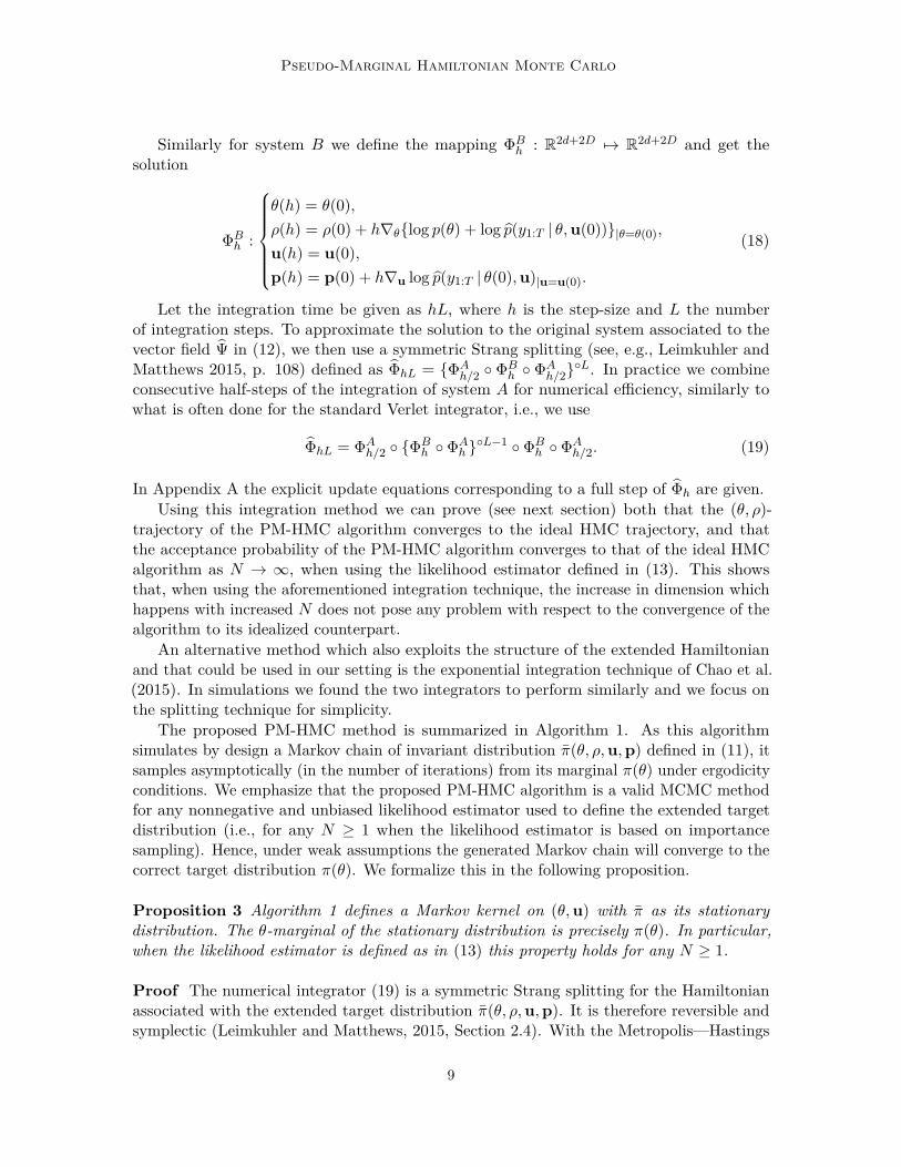
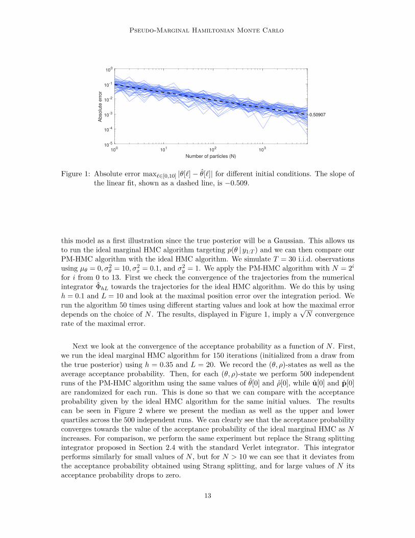
Figure 1: Absolute error max`∈[0,10] |θ[`]− θ[`]| for different initial conditions. The slope ofthe linear fit, shown as a dashed line, is −0.509.
this model as a first illustration since the true posterior will be a Gaussian. This allows usto run the ideal marginal HMC algorithm targeting p(θ | y1:T ) and we can then compare ourPM-HMC algorithm with the ideal HMC algorithm. We simulate T = 30 i.i.d. observationsusing µθ = 0, σ2
θ = 10, σ2x = 0.1, and σ2
y = 1. We apply the PM-HMC algorithm with N = 2ifor i from 0 to 13. First we check the convergence of the trajectories from the numericalintegrator ΦhL towards the trajectories for the ideal HMC algorithm. We do this by usingh = 0.1 and L = 10 and look at the maximal position error over the integration period. Werun the algorithm 50 times using different starting values and look at how the maximal errordepends on the choice of N . The results, displayed in Figure 1, imply a
√N convergence
rate of the maximal error.
Next we look at the convergence of the acceptance probability as a function of N . First,we run the ideal marginal HMC algorithm for 150 iterations (initialized from a draw fromthe true posterior) using h = 0.35 and L = 20. We record the (θ, ρ)-states as well as theaverage acceptance probability. Then, for each (θ, ρ)-state we perform 500 independentruns of the PM-HMC algorithm using the same values of θ[0] and ρ[0], while u[0] and p[0]are randomized for each run. This is done so that we can compare with the acceptanceprobability given by the ideal HMC algorithm for the same initial values. The resultscan be seen in Figure 2 where we present the median as well as the upper and lowerquartiles across the 500 independent runs. We can clearly see that the acceptance probabilityconverges towards the value of the acceptance probability of the ideal marginal HMC as Nincreases. For comparison, we perform the same experiment but replace the Strang splittingintegrator proposed in Section 2.4 with the standard Verlet integrator. This integratorperforms similarly for small values of N , but for N > 10 we can see that it deviates fromthe acceptance probability obtained using Strang splitting, and for large values of N itsacceptance probability drops to zero.
13

Alenlov, Doucet and Lindsten
100 101 102 103
Number of particles (N)
0
0.1
0.2
0.3
0.4
0.5
0.6
0.7
Acce
pta
nce
pro
ba
bili
ty
Strang
Verlet
Figure 2: Acceptance probability of the PM-HMC algorithm as a function of N in theGaussian example, averaged over 150 MCMC iterations. The solid line is themedian and the dashed lines the lower and upper quartiles over 500 independentruns. The blue lines correspond to using the Strang splitting integrator fromSection 2.4 and the brown lines to the standard Verlet integrator. The thickblack dashed line is the average acceptance probability of the ideal marginal HMCalgorithm.
4.2 Diffraction Model
Consider a hierarchical model of the form Xk | θi.i.d.∼ N (µ, σ2) and Yk | (Xk = xk), θ ∼
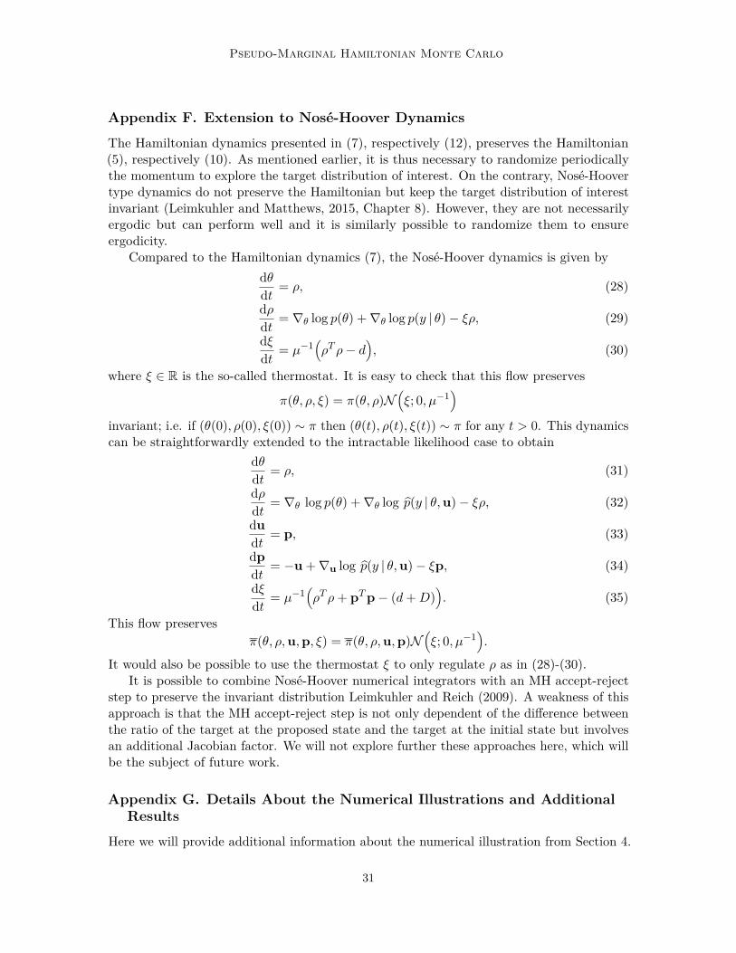
g(· |xk, λ), with θ = (µ, log(σ), log(λ)), where the observation density is modelled as adiffraction intensity: g(y |x, λ) = (λπ)−1 sinc2(λ−1(y − x)). We simulate T = 100 i.i.d.observations using µ = 1, σ = 1, and λ = 0.1. We apply the PM-HMC with N ranging from16 to 256, using a non-centered parameterization and the prior as importance density, as wellas a standard HMC working on the joint space using the same non-centered parameterization.2For further comparison we also ran, (i) a standard pseudo-marginal MH algorithm usingN = 512 and N = 1024 (smaller N resulted in very sticky behavior), (ii) the pseudo-marginalslice sampler by Murray and Graham (2016) with N ranging from 16 to 256, and (iii) a Gibbssampler akin to the Particle Gibbs algorithm by Andrieu et al. (2010) (using independentconditional importance sampling kernels to update the latent variables).
Figure 3 shows scatter plots from 40 000 iterations (after a burn-in of 10 000) for theparameters (σ, λ) for standard HMC, PM-HMC (N = 16), and pseudo-marginal slice sampling(N = 128, smaller values gave very poor mixing). Results for the remaining methods/settings,including the pseudo-marginal MH method and the Particle Gibbs sampler which bothperformed very poorly, are given in the appendix. For the pseudo-marginal slice samplingwe ran a SS+MH algorithm, where we use a random walk for the θ variables and ellipticalslice sampling for the u-variables. It is clear from the results that standard HMC fails andgenerated chains which do not mix. This is not surprising, since the diffraction intensity
2. The standard HMC, here, is equivalent to PM-HMC with N = 1. Specifically, it operates on the joint,non-centered (θ,u) space, and it uses the splitting integrator described in Section 2.4.
14
Pseudo-Marginal Hamiltonian Monte Carlo
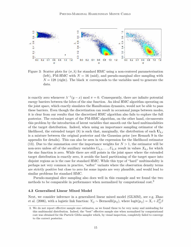
Figure 3: Scatter plots for (σ, λ) for standard HMC using a non-centered parameterisation(left), PM-HMC with N = 16 (mid), and pseudo-marginal slice sampling withN = 128 (right). The black × corresponds to the variables used to generate thedata.
is exactly zero whenever λ−1(y − x) mod π = 0. Consequently, there are infinite potentialenergy barriers between the lobes of the sinc function. An ideal HMC algorithm operating onthe joint space, which exactly simulates the Hamiltonian dynamics, would not be able to passthese barriers. Even though the discretization can result in occasional jumps between modes,it is clear from our results that the discretized HMC algorithm also fails to explore the fullposterior. The extended target of the PM-HMC algorithm, on the other hand, circumventsthis problem by the introduction of latent variables that smooth out the hard multimodalitiesof the target distribution. Indeed, when using an importance sampling estimator of thelikelihood, the extended target (8) is such that, marginally, the distribution of each Uk,i
is a mixture between the original posterior and the Gaussian prior (see Remark 9 in theappendix for details). This can also be seen in the expression for the likelihood estimator(13). Due to the summation over the importance weights for N > 1, the estimator will benon-zero unless all of the auxiliary variables Uk,1, . . . , Uk,N result in values Xk,i for whichthe sinc function is zero. While there are still points in the joint space where the extendedtarget distribution is exactly zero, it avoids the hard partitioning of the target space intodisjoint regions as is the case for standard HMC. While this type of “hard” multimodality isperhaps not very common in practice, “softer” variants where the observation density termsare strictly positive but close to zero for some inputs are very plausible, and would lead tosimilar problems for standard HMC.
Pseudo-marginal slice sampling also does well in this example and we found the twomethods to be comparable in performance when normalized by computational cost.3
4.3 Generalized Linear Mixed Model
Next, we consider inference in a generalized linear mixed model (GLMM), see e.g. Zhaoet al. (2006), with a logistic link function: Yij ∼ Bernoulli(pij), where logit(pij) = Xi +ZT
ijβ
3. We do not report effective sample size estimates, as we found these to be very noisy and misleading forthis multimodal distribution. Indeed, the “best” effective sample size when normalized by computationalcost was obtained for the Particle Gibbs sampler which, by visual inspection, completely failed to convergeto the correct posterior.
15

Alenlov, Doucet and Lindsten
for i = 1:T , j = 1:ni. Here, Yij represent the jth observation for the ith “subject”, Zij is acovariate of dimension p, β is a vector of fixed effects and Xi is a random effect for subject i.It has been recognized (Burda et al., 2008; Komarek and Lesaffre, 2008) that it is oftenbeneficial to allow for non-Gaussianity in the random effects. For instance, multimodalitycan arise as an effect of under-modelling, when effects not accounted for by the covariatesresult in a clustering of the subjects. To accommodate this we assume Xi to be distributedaccording to a Gaussian mixture: Xi
i.i.d.∼∑Kj=1wjN (µj , λ−1
j ). For simplicity we fix K = 2for this illustration. The parameters of the model are thus β, µj , λj2j=1, and w1 (asw2 = 1− w1), with X1:T being latent variables. We use the parameterisation
θ = (βT, µ1, µ2, log(λ1), log(λ2), logit(w1))T ∈ Rp+5.
We used a simulated data set with T = 500 and ni = 6, thus a total of 3 000 data points,with µ1 = 0, µ2 = 3, λ1 = 10, λ2 = 3. We set p = 8 and generate β as well the covariates Zijfrom standard normal distributions (see the appendix for further details on the simulationsetup).
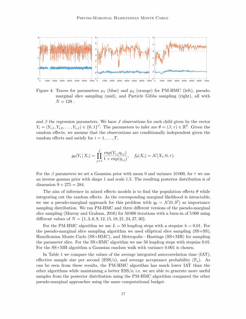
We ran PM-HMC, pseudo-marginal slice sampling (Murray and Graham, 2016), andParticle Gibbs (Andrieu et al., 2010) for 7 000 iterations, all using N = 128. We note thatGibbs sampling type algorithms (of which our Particle Gibbs sampler is an example) are thede facto standard methods for Bayesian GLMMs. For the pseudo-marginal slice sampling weused a SS+MH algorithm where for θ we have one MH step for each component and for uwe used elliptical slice sampling. Figure 4 shows traces for the parameters µ1 and µ2, withadditional results reported in the appendix. The PM-HMC method clearly outperforms thecompeting methods in terms of mixing (the computational cost per iteration is about 3.5times higher for PM-HMC than for pseudo-marginal slice sampling in our implementation).In particular, compared to the results of Section 4.2, we note that PM-HMC handles thismore challenging model with a 13-dimensional θ much better than the pseudo-marginal slicesampling which appears here to struggle for high-dimensional θ.
However, we also note that the PM-HMC algorithm gets stuck for many iterations arounditeration 1 000 (see Figure 4). Experiments suggest that this stickiness is an issue inheritedfrom the marginal HMC (which PM-HMC mimics) and is not specific to the PM-HMCalgorithm. Specifically, we have experienced that the PM-HMC sampler tends to get stuckat large values of λ1 or λ2, i.e., in the right tail of the posterior for one of these parameters.A potential solution to address this issue is to use a state-dependent mass matrix as in theRiemannian manifold HMC (Girolami and Calderhead, 2011).
4.4 Respiratory Infection Data
As a final example we consider a version of the generalized linear mixed model fromSection 4.3 applied to a real-world data set. This data set is a subset of a cohort study of275 Indonesian preschool children with 1200 observations. It has previously been studiedby Zeger and Karim (1991) using Bayesian mixed models and Schmon et al. (2021) withthe model used here. The probability of a respiratory infection is modeled based on 7covariates: age, sex, height, an indicator for vitamin deficiency, an indicator for subnormalheight and two seasonal components. A linear regression model based on the covariatesZi,j is ηi,j = ZT
i,jβ + Xi, where Xi ∼ N (0, τ) denotes the intercept for child i = 1, . . . , T
16
Pseudo-Marginal Hamiltonian Monte Carlo
0 1000 2000 3000 4000 5000 6000 7000-2
0
2
4
6
0 1000 2000 3000 4000 5000 6000 7000-1
0
1
2
3
4
5
6
0 1000 2000 3000 4000 5000 6000 7000-1
0
1
2
3
4
5
Figure 4: Traces for parameters µ1 (blue) and µ2 (orange) for PM-HMC (left), pseudo-marginal slice sampling (mid), and Particle Gibbs sampling (right), all withN = 128 .
and β the regression parameters. We have J observations for each child given by the vectorYi = (Yi,1, Yi,2, . . . , Yi,J) ∈ 0, 1J . The parameters to infer are θ = (β, τ) ∈ R9. Given therandom effects, we assume that the observations are conditionally independent given therandom effects and satisfy for i = 1, . . . , T ,
gθ(Yi |Xi) =J∏j=1
exp(Yi,jηi,j)1 + exp(ηi,j)
, fθ(Xi) = N (Xi; 0, τ).
For the β parameters we set a Gaussian prior with mean 0 and variance 10 000, for τ we usean inverse gamma prior with shape 1 and scale 1.5. The resulting posterior distribution is ofdimension 9 + 275 = 284.
The aim of inference in mixed effects models is to find the population effects θ whileintegrating out the random effects. As the corresponding marginal likelihood is intractable,we use a pseudo-marginal approach for this problem with qθ = N (0, 32) as importancesampling distribution. We ran PM-HMC and three different versions of the pseudo-marginalslice sampling (Murray and Graham, 2016) for 50 000 iterations with a burn-in of 5 000 usingdifferent values of N = 1, 3, 6, 9, 12, 15, 18, 21, 24, 27, 30.
For the PM-HMC algorithm we use L = 50 leapfrog steps with a stepsize h = 0.01. Forthe pseudo-marginal slice sampling algorithm we used elliptical slice sampling (SS+SS),Hamiltonian Monte Carlo (SS+HMC), and Metropolis—Hastings (SS+MH) for samplingthe parameter slice. For the SS+HMC algorithm we use 50 leapfrog steps with stepsize 0.01.For the SS+MH algorithm a Gaussian random walk with variance 0.001 is chosen.
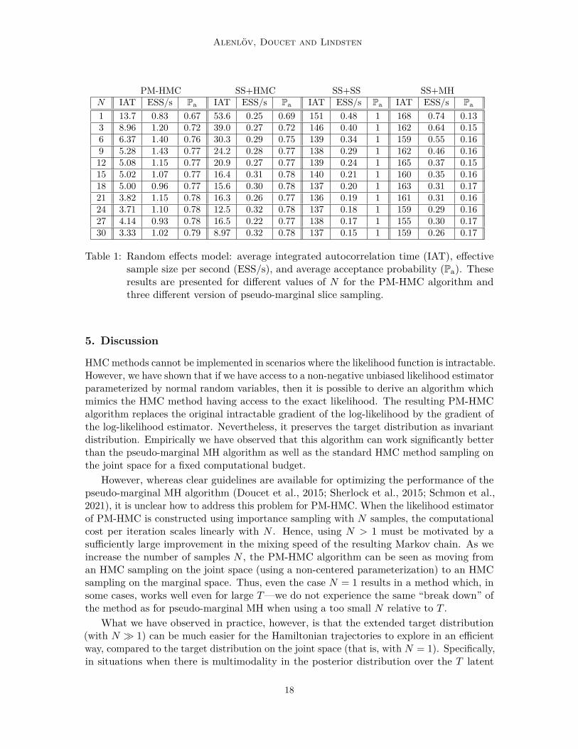
In Table 1 we compare the values of the average integrated autocorrelation time (IAT),effective sample size per second (ESS/s), and average acceptance probability (Pa). Ascan be seen from these results, the PM-HMC algorithm has much lower IAT than theother algorithms while maintaining a better ESS/s; i.e. we are able to generate more usefulsamples from the posterior distribution using the PM-HMC algorithm compared the otherpseudo-marginal approaches using the same computational budget.
17
Alenlov, Doucet and Lindsten
PM-HMC SS+HMC SS+SS SS+MHN IAT ESS/s Pa IAT ESS/s Pa IAT ESS/s Pa IAT ESS/s Pa
1 13.7 0.83 0.67 53.6 0.25 0.69 151 0.48 1 168 0.74 0.133 8.96 1.20 0.72 39.0 0.27 0.72 146 0.40 1 162 0.64 0.156 6.37 1.40 0.76 30.3 0.29 0.75 139 0.34 1 159 0.55 0.169 5.28 1.43 0.77 24.2 0.28 0.77 138 0.29 1 162 0.46 0.1612 5.08 1.15 0.77 20.9 0.27 0.77 139 0.24 1 165 0.37 0.1515 5.02 1.07 0.77 16.4 0.31 0.78 140 0.21 1 160 0.35 0.1618 5.00 0.96 0.77 15.6 0.30 0.78 137 0.20 1 163 0.31 0.1721 3.82 1.15 0.78 16.3 0.26 0.77 136 0.19 1 161 0.31 0.1624 3.71 1.10 0.78 12.5 0.32 0.78 137 0.18 1 159 0.29 0.1627 4.14 0.93 0.78 16.5 0.22 0.77 138 0.17 1 155 0.30 0.1730 3.33 1.02 0.79 8.97 0.32 0.78 137 0.15 1 159 0.26 0.17
Table 1: Random effects model: average integrated autocorrelation time (IAT), effectivesample size per second (ESS/s), and average acceptance probability (Pa). Theseresults are presented for different values of N for the PM-HMC algorithm andthree different version of pseudo-marginal slice sampling.
5. Discussion
HMC methods cannot be implemented in scenarios where the likelihood function is intractable.However, we have shown that if we have access to a non-negative unbiased likelihood estimatorparameterized by normal random variables, then it is possible to derive an algorithm whichmimics the HMC method having access to the exact likelihood. The resulting PM-HMCalgorithm replaces the original intractable gradient of the log-likelihood by the gradient ofthe log-likelihood estimator. Nevertheless, it preserves the target distribution as invariantdistribution. Empirically we have observed that this algorithm can work significantly betterthan the pseudo-marginal MH algorithm as well as the standard HMC method sampling onthe joint space for a fixed computational budget.
However, whereas clear guidelines are available for optimizing the performance of thepseudo-marginal MH algorithm (Doucet et al., 2015; Sherlock et al., 2015; Schmon et al.,2021), it is unclear how to address this problem for PM-HMC. When the likelihood estimatorof PM-HMC is constructed using importance sampling with N samples, the computationalcost per iteration scales linearly with N . Hence, using N > 1 must be motivated by asufficiently large improvement in the mixing speed of the resulting Markov chain. As weincrease the number of samples N , the PM-HMC algorithm can be seen as moving froman HMC sampling on the joint space (using a non-centered parameterization) to an HMCsampling on the marginal space. Thus, even the case N = 1 results in a method which, insome cases, works well even for large T—we do not experience the same “break down” ofthe method as for pseudo-marginal MH when using a too small N relative to T .
What we have observed in practice, however, is that the extended target distribution(with N 1) can be much easier for the Hamiltonian trajectories to explore in an efficientway, compared to the target distribution on the joint space (that is, with N = 1). Specifically,in situations when there is multimodality in the posterior distribution over the T latent
18
Pseudo-Marginal Hamiltonian Monte Carlo
variables,4 standard HMC on the joint space of parameters and latent variables can easily getstuck in local modes. In such situations, the extended target distribution used by PM-HMCis a way to bridge between the modes, as illustrated empirically by Nemeth et al. (2019).Indeed, as our theoretical analysis shows, the performance of PM-HMC will converge to thatof an ideal marginal HMC, for which the latent variables have been marginalized out, as Nbecomes large.
This explains the large improvement in performance of PM-HMC compared to standardHMC in the examples of Sections 4.2 and 4.3, which have multimodal posteriors. However,for the example studied in Section 4.4, which does not have a multimodal posterior, we alsoobserved an improvement in using N > 1. We believe that this is largely due to the fact that,in practice, the computational time does not grow linearly with N , due to a computationaloverhead that can be amortized over multiple samples when using N > 1. For instance, inour implementation, going from N = 1 to N = 30 only increased the computational timeby a factor 3.5 (see Table 1). Furthermore, modern computing architectures allow for ahigh degree of parallelization over multiple samples, which could further improve the resultsof PM-HMC with N > 1 (for instance, we did not make use of GPU acceleration in ourexperiments). Nevertheless, in practice the number of samples N is a tuning parameter thatneeds to be chosen based on the geometry of the target posterior and traded off with thecomputational cost of the method.
Finally, for brevity of presentation, we have restricted ourselves here to the pseudo-marginal approximation of a standard HMC algorithm using a constant mass matrix and aVerlet scheme. However, we believe that the same ideas can be extended to more sophisticatedHMC schemes such as the Riemannian manifold HMC (Girolami and Calderhead, 2011) orschemes discretizing the associated Nose—Hoover dynamics, as described in the appendix.
Acknowledgments
We thank Anthony Caterini for his invaluable help with implementing the random effectsmodel example. Arnaud Doucet’s research is supported by the UK Engineering and PhysicalSciences Research Council, grants EP/R034710/1 and EP/R013616/1. Fredrik Lindsten’s re-search is supported by the Swedish Research Council via the projects Learning of Large-ScaleProbabilistic Dynamical Models (contract number: 2016-04278) and Handling Uncertaintyin Machine Learning Systems (contract number: 2020-04122), by the Swedish Foundationfor Strategic Research via the project Probabilistic Modeling and Inference for MachineLearning (contract number: ICA16-0015) by the Wallenberg AI, Autonomous Systems andSoftware Program (WASP) funded by the Knut and Alice Wallenberg Foundation, and byELLIIT.
4. Even for bimodal marginals we could very well have 2T modes in the joint posterior.
19

Alenlov, Doucet and Lindsten
Appendix A. The One Step Integrator
We define Θ[`] as the full parameter vector associated with the PM-HMC algorithm after `steps of the integrator. We let Θ[0] be the initial values of the full parameter vector.
Taking one step of the integrator Φh = ΦAh/2 ΦB
h ΦAh/2 (where ΦA
h and ΦBh is given
in Equation 17 and 18) gives us the updating scheme from Θ[`] = (θ[`], ρ[`], u[`], p[`]) toΘ[`+ 1] through the following equations,
θ[`+ 1] = θ[`] + hρ[`] + h2
2 ∇θ
log p(θ) + log p(y | θ, p[`] sin(h2 ) + u[`] cos(h2 ))| θ=θ[`]+h
2 ρ[`],
ρ[`+ 1] = ρ[`] + h∇θ
log p(θ) + log p(y | θ, p[`] sin(h2 ) + u[`] cos(h2 ))| θ=θ[`]+h
2 ρ[`],
u[`+ 1] = p[`] sin(h) + u[`] cos(h) + sin(h2 )h∇u log p(y | θ[`] + h2 ρ[`],u)
|u=p[`] sin(h2 )+u[`] cos(h2 ),
p[`+ 1] = p[`] cos(h)− u[`] sin(h) + cos(h2 )h∇u log p(y | θ[`] + h2 ρ[`],u)
|u=p[`] sin(h2 )+u[`] cos(h2 ).
The steps in between are omitted but can easily be checked. Some use of trigonometricidentities has to be used to reach the final expressions.
Appendix B. Convergence of Simulated Trajectories
Lemma 7 Let f, f : Rn → Rn be continuous functions and let x, x : N→ RN be the solutionto the following difference equation:
x[i+ 1]− x[i] = h · f(x[i]), x[i+ 1]− x[i] = h · f(x[i]), (20)
both initialized using x[0] = x[0]. If f is Lipschitz with constant L then, for any ` ∈ N
‖x[`]− x[`]‖ ≤`−1∑i=0
h(1 + hL)`−(i+1)‖f(x[i])− f(x[i])‖ (21)
Proof Using (20) the proof is straightforward,
‖x[i+ 1]− x[i+ 1]‖ = ‖x[i] + h · f(x[i])− x[i]− h · f(x[i])‖≤ ‖x[i]− x[i]‖+ h‖f(x[i])− f(x[i])‖= ‖x[i]− x[i]‖+ h‖f(x[i])− f(x[i]) + f(x[i])− f(x[i])‖≤ ‖x[i]− x[i]‖+ h‖f(x[i])− f(x[i])‖+ h‖f(x[i])− f(x[i])‖≤ ‖x[i]− x[i]‖+ hL‖x[i]− x[i]‖+ h‖f(x[i])− f(x[i])‖= (1 + hL)‖x[i]− x[i]‖+ h‖f(x[i])− f(x[i])‖.
Equation (21) then follows by repeating the recursion.
For the proof of Proposition 4 we have to compare the result of the ideal HMC algorithmwith our proposed PM-HMC algorithm. Since they live on different spaces we augment
20
Pseudo-Marginal Hamiltonian Monte Carlo
the ideal HMC algorithm to incorporate the u and p part in such a way that the (θ, ρ)-marginal exactly follows the ideal HMC algorithm. We do this by introducing the followingtime-stepper that will replace ΦB
t :
ΦBt :
θ(t) = θ(0),ρ(t) = ρ(0) + t∇θlog p(θ) + log p(y | θ)|θ=θ(0),
u(t) = u(0),p(t) = p(0) + t∇u log p(y | θ(0),u)|u=u(0).
This differs from ΦB by using the gradient from the exact posterior when updating ρ(t).Further we introduce Φh = ΦA
h/2 ΦBh ΦA
h/2. Using this splitting operator as numericalintegrator we have that the marginal (θ, ρ) will coincide exactly with the ideal HMCalgorithm.
Lemma 8 Let Assumption 3 hold. Also assume that ∇θ log p(θ | y) is Lipschitz with constantL0, then it follows that Φh is Lipschitz with constant L <∞ which does not depend on N .
The proof of Lemma 8 is postponed to Appendix D. Now we have all of the resultsneeded to prove the bound on the difference between the output of the PM-HMC and theHMC algorithm.
Proof [Proof of Proposition 4] Under the assumptions, Lemma 8 holds and thus Φh isLipschitz with constant L <∞.
As the space of the ideal HMC algorithm and the pseudo marginal HMC algorithm differwe cannot directly compare them. Thus we augment the space of the ideal HMC algorithmto reach the timestepper Φh = ΦA
h ΦBh ΦA
h by adding the u and p part of the PM-HMCalgorithm to the ideal HMC algorithm. Notice that this is no longer a discretization of aHamiltonian field but it leaves (θ, ρ) unchanged from the ideal HMC algorithm. Let Θ[`] =(θ[`], ρ[`], u[`], p[`]) = Φh`(Θ[0]) as above. Let Θ[`] = (θ[`], ρ[`],u[`],p[`]) = Φh`(Θ[0]). Wehave that
‖Φh(Θ[`])− Φh(Θ[`])‖
=
√h4
4 + h2‖∇θ log(p(y1:T | θ, p[`] sin(h2 ) + u[`] cos(h2 ))
p(y1:T | θ)
)‖| θ=θ[`]+h
2 ρ[`],
by the assumption that Φh is Lipschitz with constant L we have using Lemma 7 that
‖(θ[`]ρ[`]
)−(θ[`]ρ[`]
)‖ ≤ ‖Θ[`]−Θ[`]‖
≤`−1∑i=0
h(1 + hL)`−(i+1)
√h4
4 + h2
× ‖∇θ log(p(y1:T | θ, p[i] sin(h2 ) + u[i] cos(h2 ))
p(y1:T | θ)
)‖| θ=θ[`]+h
2 ρ[`].
21
Alenlov, Doucet and Lindsten
Appendix C. Proof of CLT
Remark 9 For the proof of the CLT and the coming proof of the convergence of theacceptance probability the following “trick” will be used. Assume that U = (U1, ...,UT ) ∼π(· | θ). Conditional upon θ, the Uk = (Uk,1, ...,Uk,N ) are independent across k anddistributed according to
πk(uk | θ) = 1N
N∑j=1
ψk(uk,j | θ)∏i 6=jN (uk,i; 0p, Ip),
where ψk( · | θ) := N (· ; 0p, Ip)×$θ(yk, ·). That is πk(uk | θ) is a mixture distribution wherewe choose one component j uniformly at random and sample that variable uk,j from ψk( · | θ)and the rest of the variables uk,i : i 6= j from standard Gaussian distributions. Whatcan now be done is to introduce new variables w = [w1, w2, . . . , wN ] ∼ N (0Np, INp) andw′1 ∼ ψk( · | θ). This will be used in the proofs to compute sums over the random variablesin the following way, for some function f we have that
∑j
f(uk,j)d=∑j
f(wj) + f(w′1)− f(w1).
The convergence of the right hand side is then split to deal with the sum where all randomvariables are Gaussian and the difference between a ψk( · | θ) and Gaussian distributed randomvariable, which is usually much easier then working with the left hand side.
Proof [Proof of Proposition 5] We start by proving the result for i = 0, first we assume thatu[0] ∼ N (0D, ID) and secondly we relax this assumption by assuming that u[0] ∼ π(· | θ).For ease of notation in the proof we will assume that we only have one observation (T = 1),the extension to many observations is immediate.
We assume that u[0] ∼ N (0D, ID) and let v := p[0] sin(h2 ) + u[0] cos(h2 ) then v alsofollows a N (0D, ID) distribution, since by definition we have that p[0] ∼ N (0D, ID). Nowwe write
log p(y | θ, v)− log p(y | θ) = log
1 + p(y | θ, v)− p(y | θ)p(y | θ)
= log
1 + εN (y, v; θ)√
N
,
where
εN (y, v; θ) :=√Np(y | θ, v)− p(y | θ)
p(y | θ) = 1√N
N∑i=1$θ(y, vi)− 1.
Taking the gradient with respect to θ we get that
√N∇θ log p(y | θ, v)−∇θp(y | θ) = ∇θεN (y, v; θ)
1 + εN (y, v; θ)/√N.
22

Pseudo-Marginal Hamiltonian Monte Carlo
By the definitions we have that
E[εN (y, v; θ)2] = E[( 1√N
N∑i=1$θ(y, vi)− 1)2]
= 1N
N∑i=1
N∑j=1E[$θ(y, vi)$θ(y, vj)]− E[$θ(y, vi)]− E[$θ(y, vj)] + 1
=E[$θ(y, v1)2]− 1,
where E[$θ(y, v1)2] <∞ by assumption. Under the assumption that u[0] ∼ N (0D, ID) wehave that εN (y, v; θ)/
√N
p−→ 0 by Chebyshev’s inequality. Also noting that
E[∇θεN (y, v; θ)] =√NE[∇θ$θ(y, v1)] (1)=
√N∇θE[$θ(y, v1)] = 0,
where (1) holds under the assumptions of the existence of the function g(·) such that|∇θ$θ(y,u)| < g(u) and EN [g(u)] <∞ which then allows us to interchange the differentialand integral. By the continuous mapping theorem, Slutsky’s lemma and the standard CLTapplied to ∇θεN (y, v; θ) we get the desired results.
So far we have only proven the result when the algorithm is initialized, that is u[0] ∼N (0D, ID). At stationarity we will have (θ, u) ∼ π(θ, u). Now we wish to prove the resultsunder the assumption of having reached this distribution, that is u[0] ∼ π(· | θ). We makeuse of Remark 9 and introduce the variables w ∼ N(0, ID) and w′1 ∼ ψ(· | θ).
By adding and subtracting the term associated with p[0]1 sin(h2 ) + w1 cos(h2 ), for ease ofnotation we let p[0]w,h := p[0] sin(h2 ) + w cos(h2 ) and write√N∇θ log p(y | θ, p[0] sin(h2 ) + u[0] cos(h2 ))−∇θ log p(y | θ)
=∇θεN (y, p[0] sin(h2 ) + u[0] cos(h2 ))
1 + εN (y, p[0] sin(h2 ) + u[0] cos(h2 ))/√N
d=∇θεN (y, p[0]w,h; θ) + 1√
N(∇θ$θ(y, p[0]1 sin(h2 ) + w′1 cos(h2 ))−∇θ$θ(p[0]w,h1 ))
1 + 1√NεN (y, p[0]w,h; θ) + 1
N ($θ(y, p[0]1 sin(h2 ) + w′1 cos(h2 ))−$θ(y, p[0]w,h1 )),
as previously we have that1√N∇θ$θ(y, p[0]1 sin(h2 ) + w′1 cos(h2 )) p−→ 0 as N →∞,
1N$θ(y, p[0]1 sin(h2 ) + w′1 cos(h2 )) p−→ 0 as N →∞,
with the same results holding when we use w1 instead of w′1. By the continuous mappingtheorem and Slutsky’s lemma we have the result for the initial step.
Assume now that the following results hold at iteration ` for any h > 0,
1√N
N∑i=1∇θ$θ(y, p[`]i sin(h) + u[`]i cos(h)) d−→ N (0, σ2(θ, y)), as N →∞,
1N
N∑i=1
$θ(y, p[`]i sin(h) + u[`]i cos(h)) p−→ 1, as N →∞.
23

Alenlov, Doucet and Lindsten
This gives us using Slutsky’s lemma that
√N∇θ log
(p(y | θ, p[`] sin(h) + u[`] cos(h))
p(y | θ)
)d−→ N (0, σ2(θ, y)), as N →∞.
Taking one step to iteration `+ 1 we get that
p[`+ 1] sin(h2 ) + u[`+ 1] cos(h2 )= p[`] sin(3h
2 ) + u[`] cos(3h2 ) + sin(h)h∇u log p(y | θ, u) |
u=p[`] sin(h2 )+u[`] cos(h2 ),
from the assumptions we have that $θ(y,v) > 0 and so we can use Lemma 10 and Lemma11 which gives us that, using Slutsky’s lemma
√N∇θ log
(p(y | θ, p[`+ 1] sin(h2 ) + u[`+ 1] cos(h2 ))
p(y | θ)
)d−→ N (0, σ2(θ, y)), as N →∞,
where σ2(y, θ) = E[∇θ$θ(y,u)2]. This finishes the proof.
Appendix D. Proof of Lipschitz Continuity
Proof [Proof of Lemma 8] By explicitly writing out Φh we get that
Φh(Θ) = Φh(θ, ρ,u,p)
=
θ + hρ+ h2
2 ∇θlog p(θ | y) | θ=θ+h2 ρ
ρ+ h∇θlog p(θ | y) | θ=θ+h2 ρ
p sin(h) + u cos(h) + sin(h2 )h∇u log p(y | θ + h2ρ,u) |u=p sin(h2 )+u cos(h2 )
p cos(h)− u sin(h) + cos(h2 )h∇u log p(y | θ + h2ρ,u) |u=p sin(h2 )+u cos(h2 )
,
we need to find a L such that
‖Φh(Θ)− Φh(Θ)‖ ≤ L‖Θ− Θ‖,
or equivalently find L2 such that
‖Φh(Θ)− Φh(Θ)‖2 ≤ L2‖θ − θ‖2 + ‖ρ− ρ‖2 + ‖u− u‖2 + ‖p− p‖2
.
We have that
‖Φh(Θ)− Φh(Θ)‖2
≤‖θ − θ‖2 + (1 + h2)‖ρ− ρ‖2 + 2 cos2(h)‖u− u‖+ 2 sin2(h)‖p− p‖
+(h2 + h4
4 )‖∇θ log p(θ | y)| θ=θ+h
2 ρ−∇θ log p(θ | y)
| θ=θ+h2 ρ‖2
+h2‖∇u log p(y | θ + h2ρ,u)
|u=p sin(h2 )+u cos(h2 )−∇u log p(y | θ + h
2 ρ,u)|u=p sin(h2 )+u cos(h2 )
‖2.
24
Pseudo-Marginal Hamiltonian Monte Carlo
Under the assumption that ∇θ log p(θ | y) is Lipschitz with constant L0 and assuming that∇u log p(y | θ,u) is Lipschitz with constant L1 we have that
‖Φh(Θ)− Φh(Θ)‖2
≤(1 + L20(h2 + h4
4 ) + h2L21)‖θ − θ‖2 + (1 + h2 + L2
0h2
4 (h2 + h4
4 ) + h2
4 L21)‖ρ− ρ‖2
+(2 cos2(h) + L21h
2 cos2(h2 ))‖u− u‖2 + (2 sin2(h) + L21h
2 sin2(h2 ))‖p− p‖2,
it therefore holds that Φh is Lipschitz with constant L =√
2 + h2 + L20(h2 + h4
4 ) + h2L21. It
remains to prove that ∇u log p(y | θ,u) is Lipschitz with constant L1 and that L1 does notgrow with N .
To establish this, note that we have
∥∥∥∇u log p(y|θ, u
)−∇u log p(y|θ,u)
∥∥∥≤ ‖∇u log p(y|θ, u)−∇u log p(y|θ,u)‖ (22)
+∥∥∥∇u log p
(y|θ, u
)−∇u log p(y|θ, u)
∥∥∥. (23)
Consider first term (22) (squared),
‖∇u log p(y|θ, u)−∇u log p(y|θ,u)‖2
=T∑t=1
N∑i=1
∥∥∥∇ut,i log p(yt|θ, ut)−∇ut,i log p(yt|θ,ut)∥∥∥2.
We have
∇ut,i log p(yt|θ,ut) = ωθ(yt,ut,i)∑Nj=1ωθ(yt,ut,j)
∇ut,i logωθ(yt,ut,i)
so
∥∥∥∇ut,i log p(yt|θ, ut)−∇ut,i log p(yt|θ,ut)∥∥∥2
=∥∥∥∥∥ ωθ(yt, ut,i)∑N
j=1ωθ(yt, ut,j)∇ut,i logωθ(yt, ut,i)−
ωθ(yt,ut,i)∑Nj=1ωθ(yt,ut,j)
∇ut,i logωθ(yt,ut,i)∥∥∥∥∥
2
≤∥∥∥∥∥ ωθ(yt, ut,i)∑N
j=1ωθ(yt, ut,j)
(∇ut,i logωθ(yt, ut,i)−∇ut,i logωθ(yt,ut,i)
)∥∥∥∥∥ (24)
+∥∥∥∥∥(
ωθ(yt, ut,i)∑Nj=1ωθ(yt, ut,j)
− ωθ(yt,ut,i)∑Nj=1ωθ(yt,ut,j)
)∇ut,i logωθ(yt,ut,i)
∥∥∥∥∥2
. (25)
Under the Lipschitz assumption on the gradient of the log-weight-function the term online (24) is bounded by M‖ut,i − ut,i‖. Furthermore, under the boundedness and Lipschitz
25

Alenlov, Doucet and Lindsten
assumptions on the weight function the term on line (25) is bounded by
C
∣∣∣∣∣ ωθ(yt, ut,i)∑Nj=1ωθ(yt, ut,j)
− ωθ(yt,ut,i)∑Nj=1ωθ(yt,ut,j)
∣∣∣∣∣≤ C
∣∣∣∣∣ωθ(yt, ut,i)− ωθ(yt,ut,i)∑Nj=1ωθ(yt, ut,j)
∣∣∣∣∣+ Cωθ(yt,ut,i)∑Nj=1ωθ(yt,ut,j)
∣∣∣∣∣∑Nj=1ωθ(yt,ut,j)− ωθ(yt, ut,j)∑N
j=1ωθ(yt, ut,j)
∣∣∣∣∣≤ CD
Nω‖ut,i − ut,i‖+ CD
Nω
N∑j=1‖ut,j − ut,j‖
≤ 2CDNω
N∑j=1‖ut,j − ut,j‖.
Put together we get for the term (22) (squared),
∥∥∥∇u log p(y|θ, u
)−∇u log p(y|θ,u)
∥∥∥2
≤T∑t=1
N∑i=1
M‖ut,i − ut,i‖+ 2CDNω
N∑j=1‖ut,j − ut,j‖
2
=T∑t=1
N∑i=1
M2‖ut,i − ut,i‖2 +
2CDNω
N∑j=1‖ut,j − ut,j‖
2
+ 4MCD
Nω‖ut,i − ut,i‖
N∑j=1‖ut,j − ut,j‖
=
T∑t=1
M2N∑i=1‖ut,i − ut,i‖2 +
([2CDω
]2+ 4MCD
ω
)× 1N
N∑j=1‖ut,j − ut,j‖
2
≤T∑t=1
M2N∑i=1‖ut,i − ut,i‖2 +
([2CDω
]2+ 4MCD
ω
)×
N∑j=1‖ut,j − ut,j‖2
=(M + 2CD
ω
)2‖u− u‖2,
where the inequality on the penultimate line follows from Jensen’s inequality.
Next we address the term (23). Analogously to above we have
∥∥∇u log p(y|θ′,u
)−∇u log p(y|θ,u)
∥∥2
=T∑t=1
N∑i=1
∥∥∥∇ut,i log p(yt|θ′,ut
)−∇ut,i log p(yt|θ,ut)
∥∥∥2(26)
26

Pseudo-Marginal Hamiltonian Monte Carlo
and ∥∥∥∇ut,i log p(yt|θ′,ut
)−∇ut,i log p(yt|θ,ut)
∥∥∥2
≤∥∥∥∥∥ ωθ(yt,ut,i)∑N
j=1ωθ(yt,ut,j)
(∇ut,i logωθ(yt,ut,i)−∇ut,i logωθ(yt,ut,i)
)∥∥∥∥∥+∥∥∥∥∥(
ωθ(yt,ut,i)∑Nj=1ωθ(yt,ut,j)
− ωθ(yt,ut,i)∑Nj=1ωθ(yt,ut,j)
)∇ut,i logωθ(yt,ut,i)
∥∥∥∥∥2
≤
ωθ(yt,ut,i)∑Nj=1ωθ(yt,ut,j)
M‖θ − θ‖+ C|ωθ(yt,ut,i)− ωθ(yt,ut,i)|∑N
j=1 ωθ(yt,ut,j)
+ Cωθ(yt,ut,i)∑Nj=1ωθ(yt,ut,j)
∣∣∣∑Nj=1 ωθ(yt,ut,j)− ωθ(yt,ut,j)
∣∣∣∑Nj=1 ωθ(yt,ut,j)
2
≤
ωθ(yt,ut,i)∑Nj=1ωθ(yt,ut,j)
M + CD
ω
(1N
+ ωθ(yt,ut,i)∑Nj=1ωθ(yt,ut,j)
)2
‖θ − θ‖2.
Plugging this expression into (26) we get∥∥∇u log p(y|θ′,u
)−∇u log p(y|θ,u)
∥∥2
≤T∑t=1
N∑i=1
(
ωθ(yt,ut,i)∑Nj=1ωθ(yt,ut,j)
)2
M2 + C2D2
ω2
(1N
+ ωθ(yt,ut,i)∑Nj=1ωθ(yt,ut,j)
)2
+ωθ(yt,ut,i)∑Nj=1ωθ(yt,ut,j)
2MCD
ω
(1N
+ ωθ(yt,ut,i)∑Nj=1ωθ(yt,ut,j)
)‖θ − θ‖2
≤T∑t=1
N∑i=1
ωθ(yt,ut,i)∑Nj=1ωθ(yt,ut,j)
M2 + C2D2
ω2
(1N2 +
( 2N
+ 1)
ωθ(yt,ut,i)∑Nj=1ωθ(yt,ut,j)
)
+ωθ(yt,ut,i)∑Nj=1ωθ(yt,ut,j)
2MCD
ω
( 1N
+ 1)‖θ − θ‖2
=T∑t=1
M2 + C2D2
ω2
( 1N
+ 2N
+ 1)
+ 2MCD
ω
( 1N
+ 1)‖θ − θ‖2
≤ T(M + 2CD
ω
)2‖θ − θ‖2.
It follows that ∥∥∥∇u log p(y|θ, u
)−∇u log p(y|θ,u)
∥∥∥≤(M + 2CD
ω
)‖u− u‖+
√T
(M + 2CD
ω
)‖θ − θ‖
≤ (√T + 1)×
(M + 2CD
ω
)∥∥∥∥∥(θu
)−(θu
)∥∥∥∥∥.
27

Alenlov, Doucet and Lindsten
Appendix E. Proof of Convergence of Acceptance Probability
Proof [Proof of Proposition 6] The proof is divided in two parts. In the first part, we willshow that the log-likelihood estimator log p(y | θ,u) converges to the log-likelihood log p(y | θ)as N →∞. The second part of the proof will show that the remaining u and p parts of theacceptance probability vanishes as N increases.
The first part follows by the proof of Proposition 5, see Appendix C. For completenesswe repeat that part here, we do the proof by induction to show that for all ` we have that,
log p(y | θ, u[`]) p−→ log p(y | θ), as N →∞.
It turns out that it is needed to show this result in a more general setting, that is for anyh > 0 we wish to show that
p(y | θ, p[`] sin(h) + u[`] cos(h)) p−→ p(y | θ), as N →∞. (27)
When ` = 0 we prove the result in two different settings. First we assume thatu[0] ∼ N (0D, ID) and the result is clear since (13) is just the likelihood of the importancesampling estimator under the assumption of Gaussian proposal distribution. Secondly welook at the case when u[0] ∼ π( · | θ), we again introduce the variables w′1 ∼ ψ( · | θ) andw ∼ N (0D, ID) by the use of Remark 9, we get that
p(y | θ, p[0] sin(h) + u[0] cos(h)) = 1N
N∑i=1
ωθ(p[0]i sin(h) + u[0]i cos(h))
d= 1Nωθ(p[0]1 sin(h) + w′1 cos(h)) + 1
N
N∑i=2
ωθ(p[0]i sin(h) + wi cos(h)),
here the first part converges to zero and the second part converges to the likelihood. BySlutsky’s lemma and the continuous mapping theorem we have the result.
Assume now that (27) holds for any h > 0. We then have for `+ 1 and any h′ > 0 thatmight differ from the integration step that
p(y | θ, p[`+ 1] sin(h′) + u[`+ 1] cos(h′))
= p(y | θ, p[`] sin(h′ + h) + u[`] cos(h′ + h)
+ h sin(h′ + h2 )∇u log p(y | θ,u)
|u=p[`] sin(h2 )+u[`] cos(h2 )
)= 1N
N∑i=1
ωθ(y, p[`] sin(h′ + h) + u[`] cos(h′ + h)
+ h sin(h′ + h2 )∇u log p(y | θ,u)
|u=p[`] sin(h2 )+u[`] cos(h2 )
),
which converges to p(y | θ) by Lemma 11. The result now follows by the continuous mappingtheorem.
Let us take a look at the second part. For this part we will show that
u[0]T u[0] + p[0]T p[0]− u[L]T u[L]− p[L]T p[L] p−→ 0, as N →∞.
28

Pseudo-Marginal Hamiltonian Monte Carlo
We do this by rewriting this expression using a telescoping sum to
u[0]T u[0] + p[0]T p[0]− u[L]T u[L]− p[L]T p[L]
=N∑i=1
(u[0]2i + p[0]2i − u[L]2i − p[L]2i
)
=L−1∑`=0
N∑i=1
(u[`]2i + p[`]2i − u[`+ 1]2i − p[`+ 1]2i
).
What remains to prove is that, for all `,
N∑i=1
(u[`]2i + p[`]2i − u[`+ 1]2i − p[`+ 1]2i
)p−→ 0, as N →∞.
By taking one step of the integrator we have that, see Appendix A
u[`+ 1]i = p[`]i sin(h) + u[`]i cos(h) + sin(h2 )h∇ui log p(y | θ,ui)|ui=p[`]i sin(h2 )+u[`]i cos(h2 )
p[`+ 1]i = p[`]i cos(h)− u[`]i sin(h) + cos(h2 )h∇ui log p(y | θ,ui)|ui=p[`]i sin(h2 )+u[`]i cos(h2 ),
combining these we get that, using some trigonometric equalities,
u[`+ 1]2i + p[`+ 1]2i = p[`]2i + u[`]2i + h2(∇ui log p(y | θ,ui)|ui=p[`]i sin(h2 )+u[`]i cos(h2 ))2
+ 2h(p[`]i cos(h2 ) + u[`]i sin(h2 ))∇ui log p(y | θ,ui)|ui=p[`]i sin(h2 )+u[`]i cos(h2 ).
We now need to show two results, both holding as N →∞,
(i)N∑i=1
(∇ui log p(y | θ,ui)|ui=p[`]i sin(h2 )+u[`]i cos(h2 ))2 p−→ 0,
(ii)N∑i=1
(p[`]i cos(h2 ) + u[`]i sin(h2 ))∇ui log p(y | θ,ui)|ui=p[`]i sin(h2 )+u[`]i cos(h2 )p−→ 0.
Starting with (i) we have that, by the assumptions on the weight functions, that
N∑i=1
(∇ui log p(y | θ,ui))2 ≤N∑i=1
ω2
(∑Ni=1 ω)2
C2 = ω2C
Nω2 → 0, as N →∞.
For (ii) using the same bounds related to the gradient we get∣∣∣∣∣N∑i=1
(p[`]i cos(h2 ) + u[`]i sin(h2 ))∇ui log p(y | θ,ui)∣∣∣∣∣
≤ 1N
Cω
ω
N∑i
(p[`]i cos(h2 ) + u[`]i sin(h2 )).
29
Alenlov, Doucet and Lindsten
We now need to prove that
1N
N∑i
(p[`]i cos(h2 ) + u[`]i sin(h2 )) p−→ 0, as N →∞.
We will prove this for every ` ≥ 0 and for any value of h and this will be done using a proofof induction similar to what is done in the proof of the CLT in Appendix C.
We begin when ` = 0, we have that p[0] ∼ N (0D, ID) and assume first that u[0] ∼N (0, ID). Then the result is trivial. If we instead assume that u[0] ∼ π(· | θ). We again useRemark 9 and introduce the set of variables w1 ∼ ψ(· | θ) and w2:N ∼ N (0p, Ip). We thenhave that, for any h > 0,
1N
N∑i=1
(p[0]i cos(h) + u[0]i sin(h)) d= 1N
N∑i=1
(p[0]i cos(h) + wi sin(h))
= 1N
(p[0]1 cos(h) + w1 sin(h)) + 1N
N∑i=2
(p[0]i cos(h) + wi sin(h)).
Both of these terms now converge to 0, the first part trivially does this, while the secondpart is a sum of standard Gaussian variables and by the law of large numbers this sumconverges to 0.
Assume now that for any h > 0 we have that
1N
N∑i=1
(p[`]i cos(h) + u[`]i sin(h)) p−→ 0, as N →∞.
We now look at `+ 1, by taking one step of the numerical integrator we get that, for anyh′ > 0 which may be different then the integration step length,
1N
N∑i=1
(p[`+ 1]i cos(h′) + u[`+ 1]i sin(h′))
= 1N
N∑i=1
(p[`]i sin(h+ h′) + u[`]i cos(h+ h′)
+ h sin(h2 + h′)∇ui log p(y | θ,ui) |ui=p[`]i sin(h2 )+u[`]i cos(h2 ))
= 1N
N∑i=1
(p[`]i sin(h+ h′) + u[`]i cos(h+ h′))
+ 1N
N∑i=1
h sin(h2 + h′)∇ui log p(y | θ,ui) |ui=p[`]i sin(h2 )+u[`]i cos(h2 ),
where the first term converges to 0 in probability by the induction hypothesis and the secondsum converges to 0 in probability in the same way as (i) above. This completes the proof.
30
Pseudo-Marginal Hamiltonian Monte Carlo
Appendix F. Extension to Nose-Hoover Dynamics
The Hamiltonian dynamics presented in (7), respectively (12), preserves the Hamiltonian(5), respectively (10). As mentioned earlier, it is thus necessary to randomize periodicallythe momentum to explore the target distribution of interest. On the contrary, Nose-Hoovertype dynamics do not preserve the Hamiltonian but keep the target distribution of interestinvariant (Leimkuhler and Matthews, 2015, Chapter 8). However, they are not necessarilyergodic but can perform well and it is similarly possible to randomize them to ensureergodicity.
Compared to the Hamiltonian dynamics (7), the Nose-Hoover dynamics is given bydθdt = ρ, (28)
dρdt = ∇θ log p(θ) +∇θ log p(y | θ)− ξρ, (29)
dξdt = µ−1
(ρTρ− d
), (30)
where ξ ∈ R is the so-called thermostat. It is easy to check that this flow preserves
π(θ, ρ, ξ) = π(θ, ρ)N(ξ; 0, µ−1
)invariant; i.e. if (θ(0), ρ(0), ξ(0)) ∼ π then (θ(t), ρ(t), ξ(t)) ∼ π for any t > 0. This dynamicscan be straightforwardly extended to the intractable likelihood case to obtain
dθdt = ρ, (31)
dρdt = ∇θ log p(θ) +∇θ log p(y | θ,u)− ξρ, (32)
dudt = p, (33)
dpdt = −u +∇u log p(y | θ,u)− ξp, (34)
dξdt = µ−1
(ρTρ+ pTp− (d+D)
). (35)
This flow preservesπ(θ, ρ,u,p, ξ) = π(θ, ρ,u,p)N
(ξ; 0, µ−1
).
It would also be possible to use the thermostat ξ to only regulate ρ as in (28)-(30).It is possible to combine Nose-Hoover numerical integrators with an MH accept-reject
step to preserve the invariant distribution Leimkuhler and Reich (2009). A weakness of thisapproach is that the MH accept-reject step is not only dependent of the difference betweenthe ratio of the target at the proposed state and the target at the initial state but involvesan additional Jacobian factor. We will not explore further these approaches here, which willbe the subject of future work.
Appendix G. Details About the Numerical Illustrations and AdditionalResults
Here we will provide additional information about the numerical illustration from Section 4.
31

Alenlov, Doucet and Lindsten
G.1 Diffraction Model
A normal N (0, 102) prior was used for each component of θ. We used h = 0.02 and L = 50in all cases for simplicity, resulting in average acceptance probabilities in the range 0.6—0.8.
To generate the oberservations accept-reject sampling is used to generate random variablesfrom the distribution
g(y |λ) = (λπ)−1 sinc2( yλ),
which are then moved using the simulated x. For proposal we use the following distributionon the positive part of the real line
q(y |λ) =
(2λ)−1 0 ≤ y < λ,λ
2y2 y ≥ λ,
a random sign is then given to the accepted samples to generate samples from the desireddistribution.
In Figures 5—9 below we show traces for the parameter λ (which, along with σ, was themost difficult parameter to infer) for the various samplers considered with different settings.
0 1 2 3 4 5
×104
0
0.5
1
0 1 2 3 4 5
×104
0
0.5
1
0 1 2 3 4 5
×104
0
0.5
1
0 1 2 3 4 5
×104
0
0.5
1
Figure 5: Traces for parameter λ for the PM-HMC sampler.From top left to bottomright: N = 16, N = 64, N = 128, N = 256.
32

Pseudo-Marginal Hamiltonian Monte Carlo
0 1 2 3 4 5
×104
0
0.5
1
Figure 6: Traces for parameter λ for the standard HMC sampler, using a non-centeredparameterisation. (Note that the sampler completely misses one mode of theposterior.)
0 1 2 3 4 5
×104
0
0.5
1
0 1 2 3 4 5
×104
0
0.5
1
Figure 7: Traces for parameter λ for the pseudo-marginal MH sampler with N particles.Left, N = 512. Right, N = 1024.
33
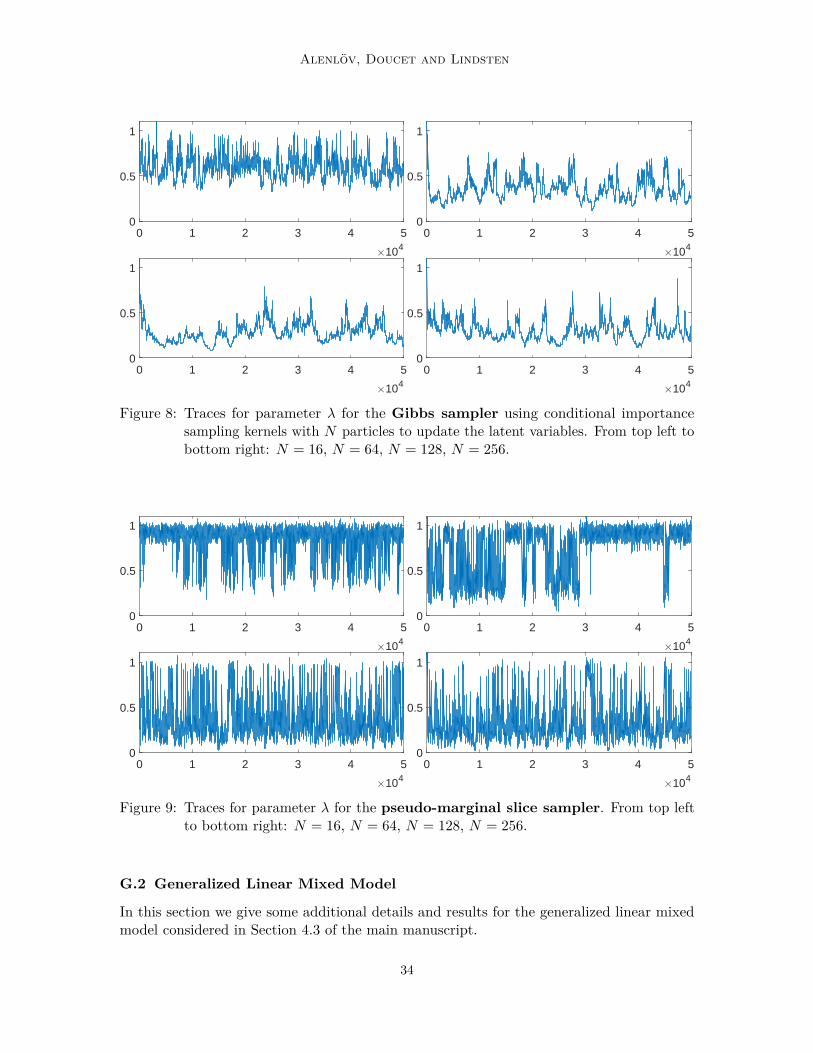
Alenlov, Doucet and Lindsten
0 1 2 3 4 5
×104
0
0.5
1
0 1 2 3 4 5
×104
0
0.5
1
0 1 2 3 4 5
×104
0
0.5
1
0 1 2 3 4 5
×104
0
0.5
1
Figure 8: Traces for parameter λ for the Gibbs sampler using conditional importancesampling kernels with N particles to update the latent variables. From top left tobottom right: N = 16, N = 64, N = 128, N = 256.
0 1 2 3 4 5
×104
0
0.5
1
0 1 2 3 4 5
×104
0
0.5
1
0 1 2 3 4 5
×104
0
0.5
1
0 1 2 3 4 5
×104
0
0.5
1
Figure 9: Traces for parameter λ for the pseudo-marginal slice sampler. From top leftto bottom right: N = 16, N = 64, N = 128, N = 256.
G.2 Generalized Linear Mixed Model
In this section we give some additional details and results for the generalized linear mixedmodel considered in Section 4.3 of the main manuscript.
34

Pseudo-Marginal Hamiltonian Monte Carlo
The parameter values used for the data generation were:
β =(−1.1671 2.4665 −0.1918 −1.0080 0.6212 0.6524 1.5410 0.2653
)T,
µ1 = 0, µ2 = 3, λ1 = 10, λ2 = 3, and w1 = 0.8.
All methods were initialized at the same point in θ-space, as follows: βinit was sampledfrom N (0p, Ip), resulting in:
βinit =(0.5838 0.3805 −1.5062 −0.0442 0.4717 −0.1435 0.6371 −0.0522
)T,
whereas the remaining parameters were initialized deterministically as µinit1 = 0, µinit
2 = 0λinit
1 = 1, λinit2 = 0.1, and winit
1 = 0.5.
We used a N (0, 100) prior for each component of θ. However, for the particle Gibbssampler we used a different parameterisation and (uninformative) conjugate priors whenpossible to ease the implementation. Varying the prior did not have any noticeable effect onthe (poor) mixing of the Gibbs sampler.
For PM-HMC and the pseudo-marginal slice sampler we used a simple (indeed, naive)choice of importance distribution for the latent variables: q(xi) = N (xi | 0, 32) since thiswas easily represented in terms of Gaussian auxiliary variables (which is a requirement forboth methods). A possibly better choice, which however we have not tried in practice,is to use a Gaussian or t-distributed approximation to the posterior distribution of thelatent variables. For the particle Gibbs sampler, which does not require the proposal to berepresented in terms of Gaussian auxiliary variables, we instead used the (slightly better)proposal consisting of sampling from the prior for Xi.
The pseudo-marginal slice sampler made use of elliptical slice sampling for updatingthe auxiliary variables, as recommended by Murray and Graham (2016). The componentsof θ were updated one-at-a-time using random walk Metropolis—Hastings kernels. Wealso updating θ jointly, but this resulted in very poor acceptance rates. The random-walkproposals were tuned to obtain acceptance rates of around 0.2—0.3.
The particle Gibbs sampler used conditional importance sampling kernels for the latentvariables X1:T , and for the parameters random walk Metropolis—Hastings kernels were usedwhen no conjugate priors were available.
Figures 10—12 show trace plots for the four parameters µ1, µ2, 1/λ1 and 1/λ2 of theGaussian mixture model used to model the distribution of the random effects. The threeplots correspond to the pseudo-marginal HMC sampler, the pseudo-marginal slice sampler,and the Gibbs sampler with conditional importance sampling kernels, respectively. InFigure 13 we show estimated autocorrelations for the 13 parameters of the model for thethree samplers.
35
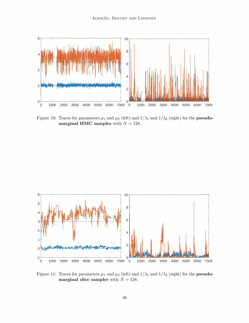
Alenlov, Doucet and Lindsten
0 1000 2000 3000 4000 5000 6000 7000-2
0
2
4
6
0 1000 2000 3000 4000 5000 6000 70000
2
4
6
8
10
Figure 10: Traces for parameters µ1 and µ2 (left) and 1/λ1 and 1/λ2 (right) for the pseudo-marginal HMC sampler with N = 128.
0 1000 2000 3000 4000 5000 6000 7000-1
0
1
2
3
4
5
6
0 1000 2000 3000 4000 5000 6000 70000
2
4
6
8
10
Figure 11: Traces for parameters µ1 and µ2 (left) and 1/λ1 and 1/λ2 (right) for the pseudo-marginal slice sampler with N = 128.
36
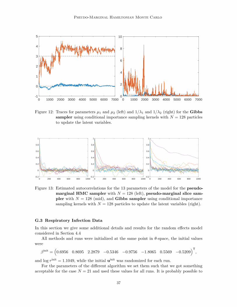
Pseudo-Marginal Hamiltonian Monte Carlo
0 1000 2000 3000 4000 5000 6000 7000-1
0
1
2
3
4
5
0 1000 2000 3000 4000 5000 6000 70000
2
4
6
8
10
Figure 12: Traces for parameters µ1 and µ2 (left) and 1/λ1 and 1/λ2 (right) for the Gibbssampler using conditional importance sampling kernels with N = 128 particlesto update the latent variables.
0 200 400 600 800 1000-0.2
0
0.2
0.4
0.6
0.8
1
0 200 400 600 800 1000-0.2
0
0.2
0.4
0.6
0.8
1
0 200 400 600 800 1000-0.2
0
0.2
0.4
0.6
0.8
1
Figure 13: Estimated autocorrelations for the 13 parameters of the model for the pseudo-marginal HMC sampler with N = 128 (left), pseudo-marginal slice sam-pler with N = 128 (mid), and Gibbs sampler using conditional importancesampling kernels with N = 128 particles to update the latent variables (right).
G.3 Respiratory Infection Data
In this section we give some additional details and results for the random effects modelconsidered in Section 4.4
All methods and runs were initialized at the same point in θ-space, the initial valueswere
βinit =(0.6956 0.8695 2.2879 −0.5346 −0.9756 −1.8065 0.5569 −0.5209
)T,
and log τ init = 1.1049, while the initial uinit was randomized for each run.For the parameters of the different algorithm we set them such that we got something
acceptable for the case N = 21 and used these values for all runs. It is probably possible to
37

Alenlov, Doucet and Lindsten
achieve better results for other values of N by tuning the parameters further. In Figure 14—16 show traces for three parameters of the β vector for the different methods and for differentvalues of N . In Figure 17 we see the average time for one iteration of the algorithm inseconds for the different methods for the different values of N used in the simulations,the simulations were done on an i7-6700k running at 4.0GHz with 16GB of memory, noGPU was used to accelerate the computations. Note the different scales on the y-axis,the pseudo-marginal slice-sampling with Metropolis—Hastings is the quickest while thePM-HMC and pseudo-marginal slice-sampling with HMC are the slowest methods.
0 10000 20000 30000 40000 500004
3
2
1
0
1
2
3pm_hmc with N = 1
0 10000 20000 30000 40000 500004
3
2
1
0
1
2
3ss_hmc with N = 1
0 10000 20000 30000 40000 500004
3
2
1
0
1
2
3ss_ess with N = 1
0 10000 20000 30000 40000 500004
3
2
1
0
1
2
3ss_mh with N = 1
Figure 14: Traces for parameters β1 (blue), β3 (orange), and β5 (green) when N = 1 forthe PM-HMC (top-left) pseudo-marginal slice sampler with HMC (top-right), elliptical slice sampling (bottom-left), and Metropolis—Hastings(bottom-right).
38
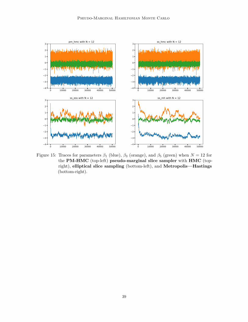
Pseudo-Marginal Hamiltonian Monte Carlo
0 10000 20000 30000 40000 500004
3
2
1
0
1
2
3pm_hmc with N = 12
0 10000 20000 30000 40000 500004
3
2
1
0
1
2
3ss_hmc with N = 12
0 10000 20000 30000 40000 500004
3
2
1
0
1
2
3ss_ess with N = 12
0 10000 20000 30000 40000 500004
3
2
1
0
1
2
3ss_mh with N = 12
Figure 15: Traces for parameters β1 (blue), β3 (orange), and β5 (green) when N = 12 forthe PM-HMC (top-left) pseudo-marginal slice sampler with HMC (top-right), elliptical slice sampling (bottom-left), and Metropolis—Hastings(bottom-right).
39

Alenlov, Doucet and Lindsten
0 10000 20000 30000 40000 500004
3
2
1
0
1
2
3pm_hmc with N = 30
0 10000 20000 30000 40000 500004
3
2
1
0
1
2
3ss_hmc with N = 30
0 10000 20000 30000 40000 500004
3
2
1
0
1
2
3ss_ess with N = 30
0 10000 20000 30000 40000 500004
3
2
1
0
1
2
3ss_mh with N = 30
Figure 16: Traces for parameters β1 (blue), β3 (orange), and β5 (green) when N = 30 forthe PM-HMC (top-left) pseudo-marginal slice sampler with HMC (top-right), elliptical slice sampling (bottom-left), and Metropolis—Hastings(bottom-right).
40
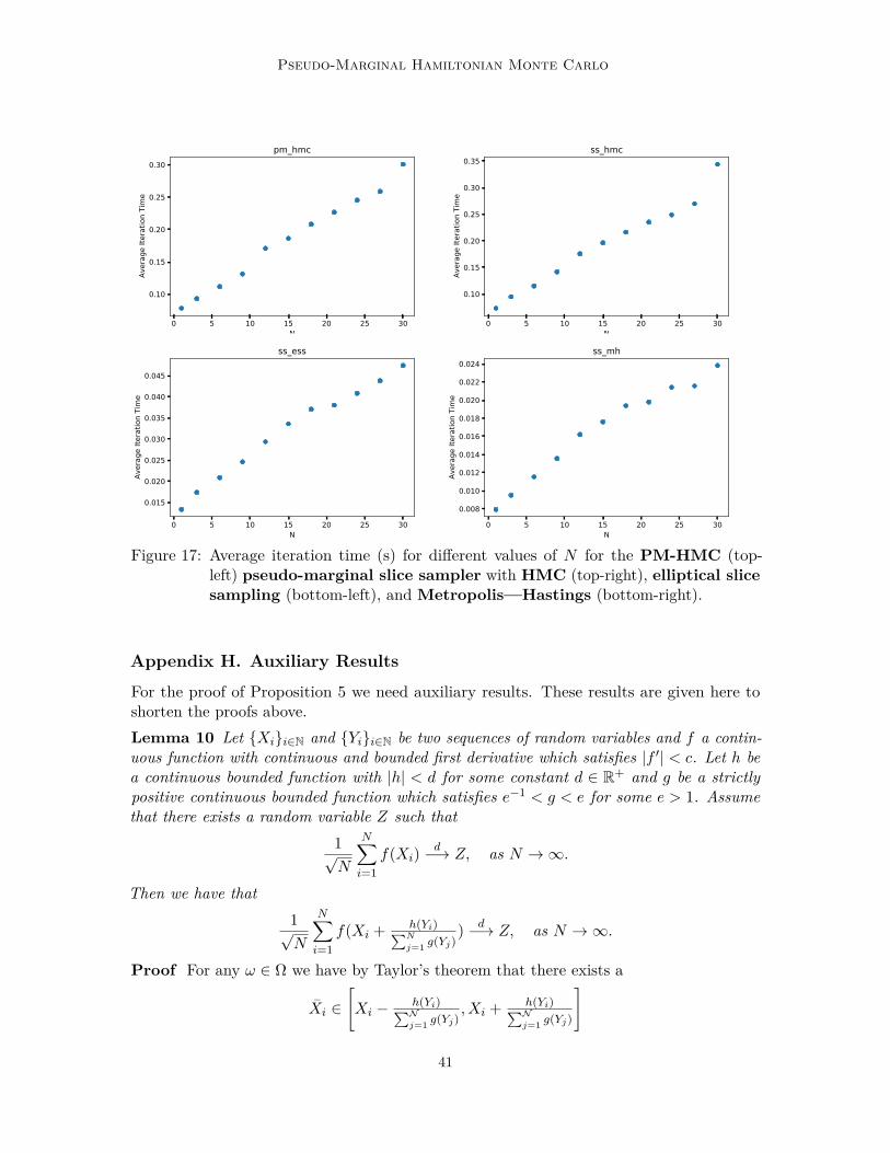
Pseudo-Marginal Hamiltonian Monte Carlo
0 5 10 15 20 25 30N
0.10
0.15
0.20
0.25
0.30
Aver
age
Itera
tion
Tim
epm_hmc
0 5 10 15 20 25 30N
0.10
0.15
0.20
0.25
0.30
0.35
Aver
age
Itera
tion
Tim
e
ss_hmc
0 5 10 15 20 25 30N
0.015
0.020
0.025
0.030
0.035
0.040
0.045
Aver
age
Itera
tion
Tim
e
ss_ess
0 5 10 15 20 25 30N
0.008
0.010
0.012
0.014
0.016
0.018
0.020
0.022
0.024
Aver
age
Itera
tion
Tim
e
ss_mh
Figure 17: Average iteration time (s) for different values of N for the PM-HMC (top-left) pseudo-marginal slice sampler with HMC (top-right), elliptical slicesampling (bottom-left), and Metropolis—Hastings (bottom-right).
Appendix H. Auxiliary Results
For the proof of Proposition 5 we need auxiliary results. These results are given here toshorten the proofs above.Lemma 10 Let Xii∈N and Yii∈N be two sequences of random variables and f a contin-uous function with continuous and bounded first derivative which satisfies |f ′| < c. Let h bea continuous bounded function with |h| < d for some constant d ∈ R+ and g be a strictlypositive continuous bounded function which satisfies e−1 < g < e for some e > 1. Assumethat there exists a random variable Z such that
1√N
N∑i=1
f(Xi)d−→ Z, as N →∞.
Then we have that1√N
N∑i=1
f(Xi + h(Yi)∑N
j=1 g(Yj)) d−→ Z, as N →∞.
Proof For any ω ∈ Ω we have by Taylor’s theorem that there exists a
Xi ∈[Xi − h(Yi)∑N
j=1 g(Yj), Xi + h(Yi)∑N
j=1 g(Yj)
]
41
Alenlov, Doucet and Lindsten
such that
f(Xi + h(Yi)∑N
j=1 g(Yj)) = f(Xi) + f ′(Xi) h(Yi)∑N
j=1 g(Yj).
Now we look at
1√N
N∑i=1
f(Xi + h(Yi)∑N
j=1 g(Yj)) = 1√
N
N∑i=1
f(Xi) + 1√N
N∑i=1
f ′(Xi) h(Yi)∑N
j=1 g(Yj),
where we use the results above to get the expression on the right hand side. We see thatby the assumption the first term converges in distribution to Z while the second term issomething that we need to control. From the assumptions we have that
− 1√N
N∑i=1
c·d∑N
j=1 e−1<
1√N
N∑i=1
f ′(Xi) h(Yi)∑N
j=1 g(Yj)<
1√N
N∑i=1
c·d∑N
j=1 e−1.
Since we have that
1√N
N∑i=1
c·d∑N
j=1 e−1
= 1√Nc · d · e→ 0 as N →∞,
we have that, by the sandwich property
1√N
N∑i=1
f ′(Xi) h(Yi)∑N
j=1 g(Yj)p−→ 0, as N →∞.
The proof concludes by using Slutsky’s lemma.
Lemma 11 Let Xii∈N and Yii∈N be two sequences of random variables and f a contin-uous function with continuous and bounded first derivative which satisfies |f ′| < c. Let h bea continuous bounded function with |h| < d for some constant d ∈ R+ and g be a strictlypositive continuous bounded function which satisfies e−1 < g < e for some e > 1. Assumethat there exists a constant µ such that
1N
N∑i=1
f(Xi)p−→ µ, as N →∞.
Then we have that
1N
N∑i=1
f(Xi + h(Yi)∑N
j=1 g(Yj)) p−→ µ, as N →∞.
The proof of this is analogous to the previous proof and is therefore omitted.
42
Pseudo-Marginal Hamiltonian Monte Carlo
References
C. Andrieu and G.O. Roberts. The pseudo-marginal approach for efficient Monte Carlocomputations. The Annals of Statistics, 37(2):697–725, 2009.
C. Andrieu, A. Doucet, and R. Holenstein. Particle Markov chain Monte Carlo methods (withdiscussion). Journal of the Royal Statistical Society: Series B (Statistical Methodology),72(3):269–342, 2010.
M.A. Beaumont. Estimation of population growth or decline in genetically monitoredpopulations. Genetics, 164(3):1139–1160, 2003.
A. Beskos, F.J. Pinski, J.M. Sanz-Serna, and A.M. Stuart. Hybrid Monte Carlo on Hilbertspaces. Stochastic Processes and their Applications, 121(10):2201–2230, 2011.
M. Betancourt and M. Girolami. Hamiltonian Monte Carlo for hierarchical models. InCurrent Trends in Bayesian Methodology with Applications, pages 79–101. Chapman &Hall / CRC Press, 2015.
M. Burda, M. Harding, and J. Hausman. A Bayesian mixed logit–probit model for multino-mial choice. Journal of Econometrics, 147(2):232–246, 2008.
W.L. Chao, J. Solomon, D. Michels, and F. Sha. Exponential integration for HamiltonianMonte Carlo. In Proceedings of the 32nd International Conference on Machine Learning,pages 1142–1151, 2015.
T. Chen, E.B. Fox, and C. Guestrin. Stochastic gradient Hamiltonian Monte Carlo. InInternational Conference on Machine Learning, pages 1683–1691, 2014.
K.D. Dang, M. Quiroz, R. Kohn, M.N. Tran, and M. Villani. Hamiltonian Monte Carlo withenergy conserving subsampling. Journal of Machine Learning Research, 20(100):1–31,2019.
G. Deligiannidis, A. Doucet, and M.K. Pitt. The correlated pseudomarginal method. Journalof the Royal Statistical Society: Series B (Statistical Methodology), 80(5):839–870, 2018.
N. Ding, Y. Fang, R. Babbush, C. Chen, R.D. Skeel, and H. Neven. Bayesian sampling usingstochastic gradient thermostats. In Advances in Neural Information Processing Systems,pages 3203–3211, 2014.
A. Doucet, M.K. Pitt, G. Deligiannidis, and R. Kohn. Efficient implementation of Markovchain Monte Carlo when using an unbiased likelihood estimator. Biometrika, 102(2):295–313, 2015.
S. Duane, A.D. Kennedy, B.J. Pendleton, and D. Roweth. Hybrid Monte Carlo. PhysicsLetters B, 195(2):216–222, 1987.
T. Flury and N. Shephard. Bayesian inference based only on simulated likelihood: particlefilter analysis of dynamic economic models. Econometric Theory, 27(5):933–956, 2011.
43

Alenlov, Doucet and Lindsten
M. Girolami and B. Calderhead. Riemann manifold Langevin and Hamiltonian Monte Carlomethods. Journal of the Royal Statistical Society: Series B (Statistical Methodology), 73(2):123–214, 2011.
M.M. Graham and A.J. Storkey. Asymptotically exact inference in differentiable generativemodels. Electronic Journal of Statistics, 11(2):5105 – 5164, 2017.
P.E. Jacob, F. Lindsten, and T.B. Schon. Smoothing with couplings of conditional particlefilters. Journal of the American Statistical Association, 115(530):721–729, 2020.
A. Komarek and E. Lesaffre. Generalized linear mixed model with a penalized Gaussianmixture as a random effects distribution. Computational Statistics and Data Analysis, 52(7):3441–3458, 2008.
B. Leimkuhler and S. Reich. A Metropolis adjusted Nose-Hoover thermostat. ESAIM:Mathematical Modelling and Numerical Analysis, 43(4):743–755, 2009.
B. Leimkuhler and X. Shang. Adaptive thermostats for noisy gradient systems. SIAMJournal on Scientific Computing, 38(2):A712–A736, 2016.
B.J. Leimkuhler and C. Matthews. Molecular Dynamics with Deterministic and StochasticNumerical Methods. Springer, 2015.
L. Lin, K.F. Liu, and J. Sloan. A noisy Monte Carlo algorithm. Physical Review D, 61(7):074505, 2000.
E. Meeds, R. Leenders, and M. Welling. Hamiltonian ABC. In Proceedings of the 31stconference on Uncertainty in Artificial Intelligence, pages 582–591, 2015.
I. Murray and M.M. Graham. Pseudo-marginal slice sampling. In Proceedings of the 19thInternational Conference on Artificial Intelligence and Statistics, pages 911–919, 2016.
I. Murray, R.P. Adams, and D.J.C. MacKay. Elliptical slice sampling. In InternationalConference on Artificial Intelligence and Statistics, volume 9, pages 541–548, 2010.
R.M. Neal. Slice sampling. The Annals of Statistics, 31(3):705–767, 2003.
R.M. Neal. MCMC using Hamiltonian dynamics. In Handbook of Markov chain MonteCarlo, pages 113–162. Chapman & Hall / CRC Press, 2011.
C. Nemeth, F. Lindsten, M. Filippone, and J. Hensman. Pseudo-extended Markov chainMonte Carlo. In Advances in Neural Information Processing Systems, pages 4314–4324,2019.
K.K. Osmundsen, T.S. Kleppe, and R. Liesenfeld. Pseudo-marginal Hamiltonian MonteCarlo with efficient importance sampling. arXiv preprint arXiv:1812.07929, 2018.
M. Quiroz, M.N. Tran, M. Villani, R. Kohn, and K.D. Dang. The block-Poisson estimatorfor optimally tuned exact subsampling MCMC. Journal of Computational and GraphicalStatistics, 2021.
44

Pseudo-Marginal Hamiltonian Monte Carlo
J.F. Richard and W. Zhang. Efficient high-dimensional importance sampling. Journal ofEconometrics, 141(2):1385 – 1411, 2007.
S.M. Schmon, G. Deligiannidis, A. Doucet, and M.K. Pitt. Large sample asymptotics of thepseudo-marginal method. Biometrika, 108(1):37–51, 2021.
B. Shahbaba, S. Lan, W.O. Johnson, and R.M. Neal. Split hamiltonian monte carlo. Statisticsand Computing, 24(3):339–349, 2014. doi: 10.1007/s11222-012-9373-1.
X. Shang, Z. Zhu, B. Leimkuhler, and A.J. Storkey. Covariance-controlled adaptive Langevinthermostat for large-scale Bayesian sampling. In Advances in Neural Information Process-ing Systems, pages 37–45, 2015.
C. Sherlock, A.H. Thiery, G.O. Roberts, and J.S. Rosenthal. On the efficiency of pseudo-marginal random walk Metropolis algorithms. The Annals of Statistics, 43(1):238–275,2015.
H. Strathmann, D. Sejdinovic, S. Livingstone, Z. Szabo, and A. Gretton. Gradient-freeHamiltonian Monte Carlo with efficient kernel exponential families. In Advances in NeuralInformation Processing Systems 28, pages 955–963, 2015.
K.E. Train. Discrete Choice Methods with Simulation. Cambridge University Press, 2009.
J. Umenberger, T. Schon, and F. Lindsten. Bayesian identification of state-space models viaadaptive thermostats. 2019.
M. Welling and Y. W. Teh. Bayesian learning via stochastic gradient Langevin dynamics.In International Conference on Machine Learning, pages 681–688, 2011.
S.L. Zeger and M.R. Karim. Generalized linear models with random effects; a Gibbs samplingapproach. Journal of the American Statistical Association, 86(413):79–86, 1991.
Y. Zhao, J. Staudenmayer, B.A. Coull, and M.P. Wand. General design Bayesian generalizedlinear mixed models. Statistical Science, 21(1):35–51, 2006.
45