arX

iv:0

806.

3652

v1 [

q-bi

o.B

M]

23

Jun

2008

Protein Structure Prediction Using Basin-Hopping

Michael C. Prentiss,

Center for Theoretical Biological Physics, University of California at San Diego,

La Jolla, CA 92093, USA

David J. Wales,

University Chemical Laboratories, Lensfield Road, Cambridge CB2 1EW,

United Kingdom

and Peter G. Wolynes

Center for Theoretical Biological Physics, University of California at San Diego,

La Jolla, CA 92093, USA

November 14, 2018

1

Abstract

Associative memory Hamiltonian structure prediction potentials are not overly rugged,

thereby suggesting their landscapes are like those of actual proteins. In the present con-

tribution we show how basin-hopping global optimization can identify low-lying minima for

the corresponding mildly frustrated energy landscapes. For small systems the basin-hopping

algorithm succeeds in locating both lower minima and conformations closer to the experimen-

tal structure than does molecular dynamics with simulated annealing. For large systems the

efciency of basin-hopping decreases for our initial implementation, where the steps consist

of random perturbations to the Cartesian coordinates. We implemented umbrella sampling

using basin-hopping to further conrm when the global minima are reached. We have also im-

proved the energy surface by employing bioinformatic techniques for reducing the roughness

or variance of the energy surface. Finally, the basin-hopping calculations have guided im-

provements in the excluded volume of the Hamiltonian, producing better structures. These

results suggest a novel and transferable optimization scheme for future energy function de-

velopment.

2

1 Introduction

The complexity of the physical interactions that guides the folding of biomolecules presents a

significant challenge for atomistic modeling. Many current protein models use a coarse grained

approach to remove degrees of freedom, such as non-polar hydrogens, which increases the fea-

sible time step in molecular dynamics simulations.1, 2 For a more dramatic improvement of the

computational efficiency solvent degrees of freedom can be reduced.3 In this case more severe

approximations can prevent the model from reproducing experimental results. Another option is

to reduce the number of degrees of freedom of the solute. The associative memory Hamiltonian

(AMH),4–6 is a coarse-grained molecular mechanics potential inspired by physical models of the

protein folding process, but flexibly incorporates bioinformatic data to predict protein structure.

The AMH is first optimised using the minimal frustration principle in terms of the Tf/Tg ratio,

which estimates the separation in energy relative to the variance for the misfolded ensemble. Along

with using the energy of the native structure to estimate Tf , a random energy model7 estimate

of the glass transition temperature, Tg, is used based on a set of decoy structures. Tg represents

a characteristic temperature scale at which kinetic trapping in misfolded states dominates the

dynamics. An improved potential is next obtained that uses better estimates of the Tf/Tg ratio

obtained by maximizing the normalized difference between the native state and a sampled set of

misfolded decoys which are self-consistently obtained from the potential itself. The potential so

obtained is transferable for the prediction of structures outside of the training set. The ratio Tf/Tg

has provided a powerful metric for the optimisation of both this bioinformatically informed energy

function,8, 9 as well as other types of energy functions incorporating only physical information.10–12

While the optimisation13 of parameters using a training set of evolved natural proteins smooths

the energy landscape from what it would be for a random hetero-polymer, the common problem

of multiple competing minima persists even when using a reasonably accurate structure prediction

potential, such as this one. Simulated annealing with molecular dynamics has previously been used

to search the rugged landscapes of optimised structure prediction potentials.14 While free energy

profiles indicate that better structures actually are present at low temperatures, the slow kinetics

3

of a glass-like transition during annealing has prevented these minima from being reached.15 To

quantitatively investigate the origin of the sampling difficulties it is desirable to use different search

strategies.

Here we implement the basin-hopping global optimisation algorithm,16–18 which has proved ca-

pable of overcoming large energetic barriers in a wide range of different systems. Basin-hopping is

an algorithm where a structural perturbation is followed by energy minimisation. This procedure

effectively transforms the potential energy surface, by removing high barriers, as shown in Fig. 1.

Moves between local minima are accepted or rejected based upon a Monte Carlo criterion. Avoid-

ing barriers by employing a numerical minimisation step not only facilitates movement between

local minima, but also broadens their occupation probability distributions, which overlap over a

wider temperature range, thereby increasing the probability of interconversion.19 Furthermore, it

does not alter the nature of the local minima since the Hamiltonian itself is not changed, enabling

the comparison between molecular dynamics and basin-hopping generated minima. This method

has previously been applied to find global minima in atomic and molecular clusters,20, 21 biopoly-

mers,22, 23 and solids.24 Since the algorithm only requires coordinates, energies, and gradients,

it can be transferred between different molecular systems such as binary Lennard-Jones clusters,

all-atom biomolecules, or coarse-grained proteins models as in this study.

2 Theory and Computational Details

The AMH energy function used in the present work has previously been optimised over a set of

non-homologous α helical proteins, and consists of a backbone term, Eback, and an interaction

term, Eint, which has an additive form.25, 26 This model is sometimes termed the AMC model

(associative memory contact) to distinguish it from one that uses nonadditive water mediated

interactions termed the AMWmodel.14, 27 Since this model has been described in detail before,15, 28

we will only summarize its form here. We employ a version of the coarse-grained model where the

twenty letter amino acid code has been reduced to four, and the number of atoms per residue is

limited to three (Cα, Cβ, and O), except for glycine residues. The units of energy and temperature

4

were both defined during the parameter optimisation. The interaction energy ǫ was defined in

terms of the native state energy excluding backbone contributions, ENamc, via

ǫ =

∣

∣ENamc

∣

∣

4N, (1)

where N is the number of residues of the protein being considered. Temperatures are quoted in

terms of the reduced temperature Tamc = kBT/ǫ. While Eback creates self-avoiding peptide-like

stereochemistry, Eint introduces the majority of the attractive interactions that produce folding.

The interactions described by Eint depend on the sequence separation |i− j|. The interaction

between residues less than 12 amino acids apart were defined by Eqs. (2).

Elocal = −ǫ

a

Nmem∑

µ=1

∑

j−12≤i≤j−3

γ(Pi, Pj, Pµi′ , P

µj′ , x(|i− j|)) exp

[

−(rij − rµi′j′)

2

2σ2ij

]

, (2)

The index µ runs over all Nmem memory proteins to which the protein has previously been aligned

using a sequence-structure threading algorithm29 (i.e. each i-j pair in the protein has an i′-j′ pair

associated with it in every memory protein; if, due to gaps in the alignment, there is no i′-j′ pair

associated with i-j for a particular memory then this memory protein simply gives no contribution

to the interaction between residues i and j). The interaction between Cα and Cβ atoms is a sum

of Gaussian wells centred at the separations rµi′j′ of the corresponding memory atoms. The widths

of the Gaussians are given by σij = |i− j|0.15 A. The scaling factor a is used to satisfy Eq. 1.

The weights given to each well are controlled by γ(Pi, Pj, Pµi′ , P

µj′ , x(|i− j|)), which depends on

the identities Pi′ and Pj′ of the residues to which i and j are aligned, as well as the identities Pi

and Pj of i and j themselves. The self-consistent optimisation calculates the γ parameter which

originates the cooperative folding in the model. A three well contact potential [Eq. (3)] is used

for residues separated by more than 12 residues as described by,

Econtact = −ǫ

a

∑

i<j−12

3∑

k=1

γ(Pi, Pj, k)ck(N)U(rmin(k), rmax(k), rij). (3)

5

Here, the sequence indices i and j sum over all pairs of Cβ atoms separated by more than 12

residues. The sum over k is over the three wells which are approximately square wells between

rmin(k) and rmax(k) defined by,

U(rmin(k), rmax(k), rij) =1

4

{[

1 + tanh(

7[rij − rmin(k)]/A)]

+[

1 + tanh(

7[rmax(k)− rij ]/A)]}

.

(4)

The parameters (rmin(k), rmax(k)), are (4.5A, 8.0A) , (8.0A, 10.0A), and (10.0A, 15.0A) for k =

1, 2 and 3 respectively. In order to approximately account for the variation of the probability

distribution of pair distances with number of residues in the protein (N) a factor ck(N) has been

included in Elong. It is given by c1 = 1.0, c2 = 1.0/(0.0065N +0.87) and c3 = 1.0/(0.042N +0.13).

The individual wells are also weighted by γ parameters which depend on the identities of the

amino acids involved, using the 4-letter code defined above. In contrast to the interactions between

residues closer in sequence, this part of the potential does not depend on the database structures

that define local-in-sequence interactions.

To pinpoint the effects of frustration or favorable non-native contacts always present in any

coarse gained protein model, we simulated a perfectly smooth energy function often called a Go

model.30 Go models are an essential tool for understanding protein folding kinetics.31, 32 While

having the same backbone terms,33 in this single structure based Hamiltonian [Eq. (5)], all of

the interactions, Eint are defined by Gaussians whose minima are located at the pair distribution

found in the experimental structure:

EAMGo = −

ǫ

aGo

∑

i≤j−3

γGo(x(|i− j|)) exp

[

−(rij − rNij)

2

2σ2ij

]

. (5)

The global minima of such an energy function should be the input structure.

Many have used additional constraining potentials to characterise unsampled regions of co-

ordinate space while using molecular dynamics.15, 34 To characterize the landscape sampled with

basin-hopping, we also used a structure constraining potential to identify ensembles with fixed

but varying fractions of native structure. Using such a potential allows us to access interesting

6

configurations that are unlikely to be thermally sampled. The constraining potential also called

umbrella potentials are centered on different values of an order parameter to sample along the

collective coordinates. One of the collective coordinates is Q, an order parameter that measures

the sequence-dependent structural similarity of two conformations by computing the normalized

summation of C-alpha pairwise contact differences, as defined in Eq. (6):15

Q =2

(N − 1)(N − 2)

∑

i<j−1

exp

[

−(rij − rNij)

2

σ2ij

]

. (6)

The resulting order parameter ranges from zero, where there is no similarity between structures,

to one, which represents an exact overlap. The form of the potential is E(Q) = 2500ǫ(Q− Qi)4,

where Qi may be varied in order to sample different regions of the chosen order parameter. As

in equilibrium sampling, simulations were initiated at the native state and the Qi parameter was

reduced throughout the sampling.

We have also studied the potential energy landscape when multiple surfaces are superimposed

upon each other by the use of multiple homologous target proteins. This manipulation of the

energy landscape has been shown to further reduce local energetic frustration that arises from

random mutations in the sequence away from the consensus optimal sequence for a given structure.

By reducing the number of non-native traps, this averaging often improves the quality of structure

prediction results.35–38 As seen in Eq. (7), the form and the parameters of the energy function are

maintained from Eqs. (2) and (3), but the normalized summation is taken over a set of homologous

sequences:

EAM = −1

Nseq

seq∑

k=1

N∑

i<j

Eint(Pki , P

kj ). (7)

Since proteins are not random heteropolymers, the differences in the energy function for homolo-

gous proteins are randomly distributed, therefore the mean over multiple energy functions should

have less energetic variation than the original function. Indeed, performing this summation is a

way of incorporating to the optimisation of the Tf/Tg criterion into any energy function. The

target sequences of the homologues can be identified using PSI-Blast with default parameters.39, 40

7

Some classes of proteins have a large number of sequence homologues, therefore performing a mul-

tiple sequence alignment can be impractical. Removing redundant sequences from within the set of

identified homologues also removes biases that can be introduced where there are few homologues

available. This is done by preventing sequences in the collected sequences from having greater

than 90% sequence identity. The remaining sequences are aligned in a multiple sequence align-

ment.41 Gaps within the sequence alignment can be addressed within the AMH energy function

in a variety of ways. In the present work, gaps in the target sequence were removed, while gaps

within homologues were completed with residues from the target protein. While this procedure

may introduce small biases toward the target sequence, it is preferable to ignoring the interactions

altogether.

Finally, we made several ad hoc changes to the backbone potential, Eback. Eliminating some

compromises necessary for rapid molecular dynamics simulations allowed the AMH potential to be

adapted to basin-hopping. Another goal was to prevent the over-collapse of the proteins by altering

the excluded volume energy term, which should reduce the number of states available during

minimisation. The terms shown in Eq. (8) are used to reproduce the peptide-like conformations

in the original molecular dynamics energy function:

Eback = Eev + Eharm + Echain + Echi + ERama. (8)

Eev maintains a sequence specific excluded volume constraint between the Cα-Cα, Cβ-Cβ, O-O,

and Cα-Cβ atoms that are separated by less than rev. Previously,26 we have seen that modifying

Eback can produce a less frustrated energy surface when using thermal equilibrium sampling, but

slow dynamics was often found to result since the local barrier heights became too large. The

ability of basin-hopping to overcome such large, but local barriers allows us therefore to consider

a potential whose dynamics would otherwise be too slow for molecular dynamics. In the final part

8

of the paper, we altered the excluded volume term, as shown in Eq. (9) to prevent over-collapse:

Eev = ǫλCRV

∑

x,y

∑

i<j

θ(rCev(j−i)−rCxiC

yj)(rCev(j−i)−rCx

iC

yj)2+ǫλO

ev

∑

i<j

θ(rOev−rOiOj)(rOev−rOiOj

)2, (9)

by changing the default molecular dynamics parameters, λCEV = 20, λO

EV = 20, rCev(j − i < 5) =

3.85 A, rCev(j − i ≥ 5) = 4.5 A, and rOev = 3.5 A, to λCEV = 250, λO

EV = 250, rCev(j − i < 5) = 3.85 A,

rCev(j − i ≥ 5) = 3.85 A, and rOev = 3.85 A. The force constant are over an order of magnitude

larger than those used in the molecular dynamics, and the radii of the Cα, Cβ , and O atoms are

also 10% larger than previously used values. This increase in excluded volume slows the onset

of chain collapse, but improves steric interactions. The other change to the backbone potential

involves terms which maintain chain connectivity. In molecular dynamics annealing, covalent

bonds are preserved using the SHAKE algorithm,42 which permits an increase of the molecular

dynamics time step. For basin-hopping in all parts of this paper, we removed the SHAKE method

and replaced it with a harmonic potential, Eharm, between the Cα-Cα, Cα-Cβ, and Cα-O atoms.

This replacement permits the location of local minima without requiring an internal coordinate

transformation, and avoids discontinuous gradients. When minimised, the additional harmonic

terms typically contribute only only .015 kBT per bond. The remaining terms of the original

backbone potential are maintained. Depending on the sidechain, the neighbouring residues in

sequence sterically limit the variety of positions the backbone atoms can occupy, as evidenced in

a Ramachandran plot.43 This distribution of coordinates is reinforced by a potential, ERama, with

artificially low barriers to encourage rapid local movements. The planarity of the peptide bond is

ensured by a harmonic potential, Echain. The chirality of the Cα centres is maintained using the

scalar triple product of neighbouring unit vectors of carbon and nitrogen bonds, Echi.

For basin-hopping simulations, whose algorithm is outlined in Fig. 2 the most important sam-

pling parameters are the temperature used in the accept/reject steps for local minima Tbh, and the

maximum step size for perturbations of the Cartesian coordinates d. A higher temperature allows

transitions to an increased energy minima to be accepted, and also creates a larger the number

of iterations typically required to minimise the greater perturbed configurations. Too high a tem-

9

perature leads to insufficient exploration of low-energy regions. The temperature (Tbh) for these

simulations was 10 Tamc. Lower temperatures resulted in slower escape rates from low energy

traps, while higher temperatures prevented adequate exploration of low energy regions. The step

size needs to be large enough to move the configuration into the basin of attraction of one local

minimum to a neighbouring one, but not be so large that the new minimum is unrelated to the

previous state. Every Cartesian coordinate was displaced up to a maximum step size(d) of 0.75 A,

the optimum value determined from preliminary tests. Each run consisted of 2500 basin-hopping

steps saving structures every 5 basin-hopping steps. The convergence condition (δEmin) on the

root-mean-square (RMS) gradient for each minimisation was set to 10−3 ǫ, and the 5 lowest-lying

minima from each run were subsequently converged more tightly (δEfinal) to an RMS gradient of

10−5ǫ. It is important to note that basin-hopping does not provide equilibrium thermodynamic

sampling. In structure prediction there, however, is no rigorous need for the search to obey de-

tailed balance since the global energy minimum is the primary interest. Basin-hopping provides

a means for the optimal global search of the energy landscape, however other methods must be

used when calculating free energy and entropy.

In previous structure prediction studies with the AMH, low energy structures were identified

using off-lattice Langevin dynamics with simulated annealing, employing a linear annealing sched-

ule of 10000 steps from a temperature of 2.0 to 0.0, starting from a random configuration.5 The

number and length of simulations needed in both strategies were determined by the number of

uncorrelated structures encountered. The current basin-hopping method with the AMC energy

function encounters roughly one deep trap per run. In order to sample 100 independent structures

in molecular dynamics 20 separate runs were needed, because simulated annealing samples about

five independent states before the glass transition temperature is encountered, as measured by the

rapid decay of structural correlations. We compared several α helical proteins, both from within

and outside the training set of the AMH energy function.

10

3 Results and Discussion

We performed initial calculations with a Go potential for the 434 repressor (protein data bank

(PDB44) ID 1r69). In Fig. 3 we show this model accurately represents the native basin. Steps

where the energy increases are allowed by the sampling method and are not examples of frustration.

Studies on the Go model provide a useful benchmark for comparing the computer time required

for the different global optimisation strategies. Using the sampling parameters used in this report,

we compared the time for initial collapse between the molecular dynamics and basin-hopping runs.

The initial collapse required about 7 minutes for the annealing runs and 31 minutes for basin-

hopping on a desktop computer. However, these values do not reflect the actual performance of

the two approaches in locating global minima, which will depend upon the move sets, step size,

temperature, and convergence criteria.

While using the AMC structure prediction Hamiltonian, we found that basin-hopping was

often able to locate lower energy structures and also identified minima that have greater structural

overlap with the native state than annealing. These results are produced for structure predictions

for proteins both inside and outside the training set, as demonstrated in Table 1. The first

three proteins (PDB ID 1r69, 3icb, 256b) in Table 1 are in the training set of the Hamiltonian25,

while the other three are not, and can therefore be considered as predictions from the algorithm.

The minima located with basin-hopping show an increase in structural overlap with the native

state [Eq. (6)] when compared to the Langevin dynamics approach. Q scores of 0.4 for single

domain proteins generally correspond to a low resolution root mean square deviation (RMSD)

of around 5 Aor better. Q scores of 0.5 and higher have still more accurate tertiary packing

and are of comparable quality to the experimentally derived models. The high quality structures

obtained suggest the form of the backbone terms is appropriate, since the physically correct

stereochemistry is reproduced. Lower energy structures are sampled by basin-hopping for the

non-training set proteins, but the structural overlap improvement found in these deeper minima

was smaller. Larger proteins pose a greater challenge for basin-hopping with this Hamiltonian due

to the random steps in Cartesian coordinates. Dihedral coordinate move steps would probably be

11

more efficient, and will be considered in future work.

The distribution of minima encountered from multiple simulations for both search methods is

shown in Fig. 4 where a greater density of high quality structures is obtained by the basin-hopping

algorithm. The potential energy surface still includes, therefore, significant residual frustration

in the near-native basin in the form of low-lying minima separated by relatively high barriers.

Without the parameter optimisation to reduce frustration, folding would exhibit more pronounced

glassy characteristics. Most of the cooperative folding occurs during collapse until Q values of

around 0.4 are reached. While the structures from simulated annealing are accurate enough for

functional determination, we see basin-hopping can better overcome barriers that are created after

collapse. The density of the high quality structures is also important for post-simulation k-means

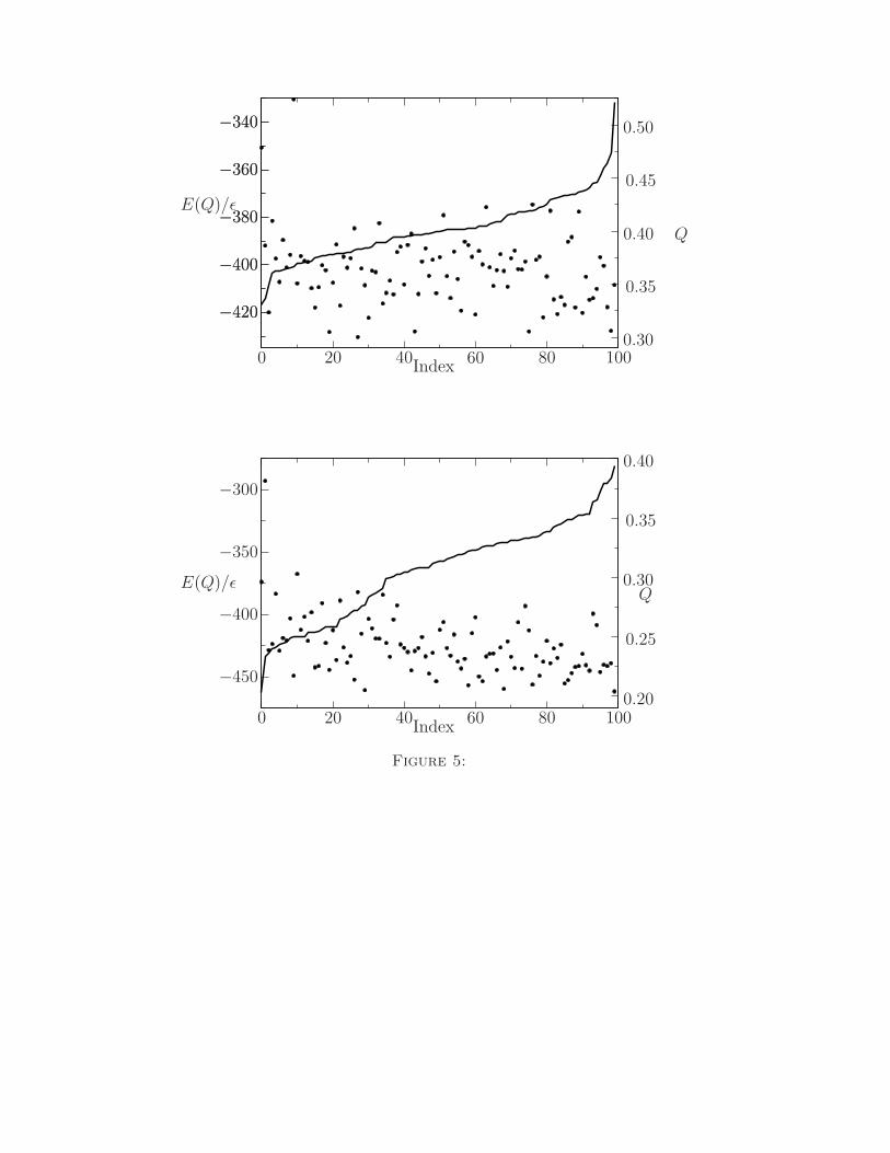
clustering analysis45. Another way of representing the data of a set of independent basin-hopping

simulations is by selecting the lowest energy structures from each simulation of the 434 repressor

(PDB ID 1r69) and HDEA (PDB ID 1bg8) proteins and ordering them with respect to their

structural overlap. As shown in Fig. 5, the protein in the training set (434 repressor) produces

better results than the non-training protein, as expected.

We have decomposed the different energy terms in the Hamiltonian in Table 2, to examine

which interactions are most effectively minimised. The AMC potential has three different dis-

tance classes in terms of sequence separation, and these are defined as short (|i− j| < 5), medium

(5 ≤ |i− j| ≤ 12), and long (|i− j| > 12). Most importantly, the long-range AMH interactions

are successfully minimised in the basin-hopping runs, due to the ability of basin-hopping to over-

come large energetic barriers. This term will govern the quality of structures sampled using an

approximately smooth energy landscape. The other terms that define secondary structure for-

mation are not as well minimised. This result is due to the disruption of helices by the random

Cartesian perturbation move steps. These move steps benefit favorable steric packing and there-

fore do well at minimising the excluded volume energy term of the Hamiltonian. A combined

minimisation approach might be more efficient, where larger dihedral steps could be made early

during minimisation to sample a wider number of structures, followed by random Cartesian steps

12

to optimise the steric interactions.

While we sampled high quality structures, we would like to confirm that we have completely

sampled the global minima of the energy surface. To access these unsampled states we used um-

brella potentials. When constraining a set of simulations to different values of Q, we have obtained

energy minima for cytochrome c, roughly 15 ǫ deeper than those from unconstrained minimisations

starting with a randomized structure, as shown in Fig. 6. For the 434 repressor the minima ob-

tained from randomized states and those found with the Q constraints applied differ by only a few

kBT . This shows basin-hopping does indeed act as a global optimisation method, by accurately

identifying the global energy minimum from multiple independent unconstrained simulation. This

behavior is predictable from the choices that governed the design of the Hamiltonian. Low energy

barriers between structures are desirable during a molecular dynamics simulation because they

accelerate the dynamics. However, for basin-hopping these low barriers encourage tertiary contact

formation before secondary structure units condense for sequences greater than 110 amino acids.

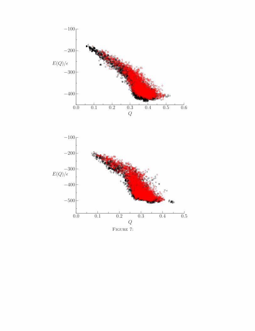
Superposition of Multiple Energy Landscapes

Constructing a Hamiltonian by calculating the arithmetic average of the potential over a set of

homologous sequences increased the quality of predictions in both equilibrium and annealing simu-

lations. We have found this approach also improved the performance in basin-hopping simulations.

For two different proteins, 100 independent basin-hopping runs were performed with both the stan-

dard and sequence-averaged Hamiltonians. By the superposition of multiple energy landscapes

we saw a reduction in the number of competing low energy traps around Q values of 0.3 for both

the 434 repressor and uteroglobin (PDB ID 1UTG), as shown in Fig. 7. Improvement of structure

prediction Hamiltonians can be statistically described by the average energy gap between the

native basin and a set of unfolded structures, and by the roughness of the energy surface, which

corresponds to the variance of the energy. The sequence based energy function summations limited

the energetic variance of the sampled landscapes, thereby reducing the glass transition temper-

ature. This improvement, even at the low temperatures sampled in basin-hopping, is predicted

13

from theory, but difficult to observe in conventional equilibrium simulations due to the emergent

glassy dynamics, which slows the kinetics. The energy gap improvement was smaller than the

reduction of the energetic variation of the Hamiltonian. In terms of the goal of maximizing the

ratio of Tf/Tg, this increase came primarily from to reducing the glass transition temperature Tg.

In the low energy region we saw fewer competing states, and an increased correlation between E

and Q for the sequence-averaged Hamiltonian compared to the original Hamiltonian. For the 434

repressor the lowest energy structure had the highest Q value encountered.

Characterisation of Polymer Collapse

When we annealed the Hamiltonian using molecular dynamics we observed some over-collapse of

the polypeptide chain, producing a smaller radius of gyration than the experimental structure.

In basin-hopping runs we also found structures exhibiting a larger number of contacts than the

experimental structure, as show in Fig. 8, where a contact is defined as a Cα-Cα distance of

less than 8 A. While the low-energy structures may be native-like, these structures were more

compact than those observed experimentally. To investigate this behavior, we examined the

backbone and interaction terms of the Hamiltonian separately using the Go Hamiltonian in Eq. (5).

Somewhat surprisingly, the Go model also produces over-collapse, as shown in Fig. 9. Hence the

interaction parameters of the structure prediction Hamiltonian were not responsible for all of

the over-collapse. These minimal model-dependent frustrations were only eliminated in the final

stages of minimisation. The most effective technique for reducing over-collapse was to increase the

force constant and the atomic radius in the excluded volume terms [Eq. (9)]. The barrier crossing

capabilities of basin-hopping steps produce more over-collapse than do the annealing minimisations

without these parameter changes. The glass-like transition seen in simulated annealing prevents

further collapse in molecular dynamics, as the rearrangement rates slow down exponentially with

temperature. The improved parameter set of Fig. 10 shows more native-like collapse, but the

lowest energy structures had Q values of 0.36 and the best Q value was 0.45, which are worse than

basin-hopping simulations with the original parameters.

14

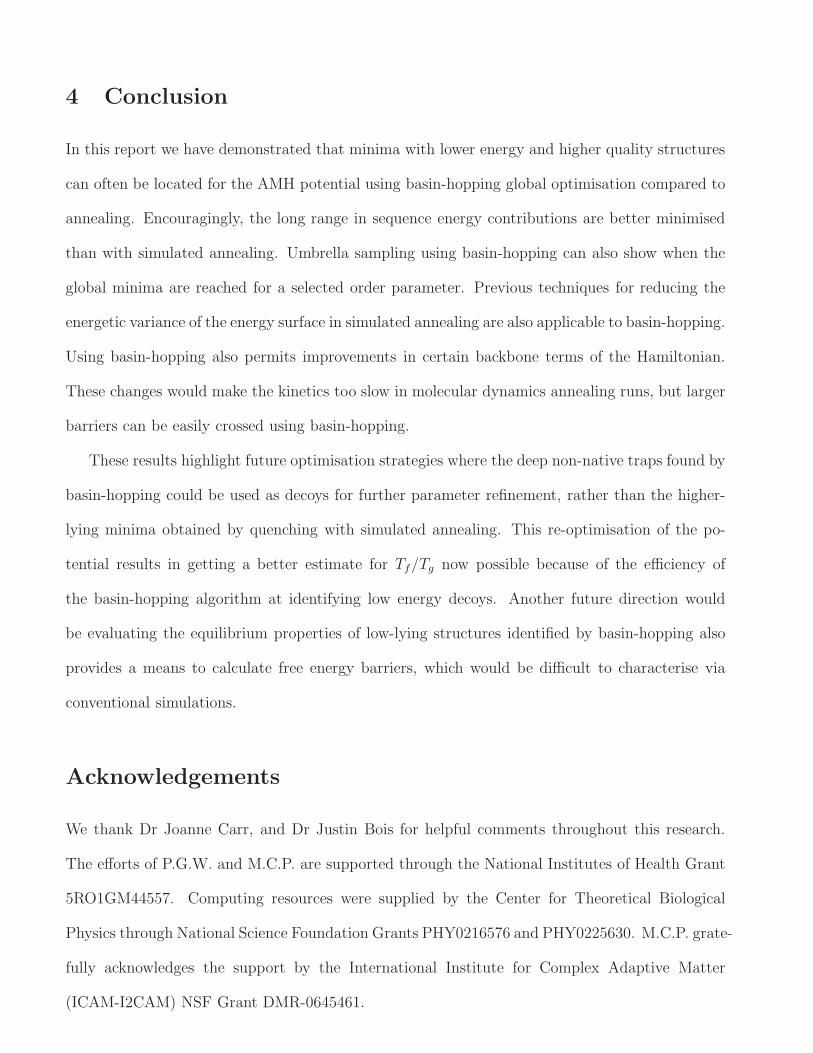
4 Conclusion

In this report we have demonstrated that minima with lower energy and higher quality structures

can often be located for the AMH potential using basin-hopping global optimisation compared to

annealing. Encouragingly, the long range in sequence energy contributions are better minimised

than with simulated annealing. Umbrella sampling using basin-hopping can also show when the

global minima are reached for a selected order parameter. Previous techniques for reducing the

energetic variance of the energy surface in simulated annealing are also applicable to basin-hopping.

Using basin-hopping also permits improvements in certain backbone terms of the Hamiltonian.

These changes would make the kinetics too slow in molecular dynamics annealing runs, but larger

barriers can be easily crossed using basin-hopping.

These results highlight future optimisation strategies where the deep non-native traps found by

basin-hopping could be used as decoys for further parameter refinement, rather than the higher-

lying minima obtained by quenching with simulated annealing. This re-optimisation of the po-

tential results in getting a better estimate for Tf/Tg now possible because of the efficiency of

the basin-hopping algorithm at identifying low energy decoys. Another future direction would

be evaluating the equilibrium properties of low-lying structures identified by basin-hopping also

provides a means to calculate free energy barriers, which would be difficult to characterise via

conventional simulations.

Acknowledgements

We thank Dr Joanne Carr, and Dr Justin Bois for helpful comments throughout this research.

The efforts of P.G.W. and M.C.P. are supported through the National Institutes of Health Grant

5RO1GM44557. Computing resources were supplied by the Center for Theoretical Biological

Physics through National Science Foundation Grants PHY0216576 and PHY0225630. M.C.P. grate-

fully acknowledges the support by the International Institute for Complex Adaptive Matter

(ICAM-I2CAM) NSF Grant DMR-0645461.

15

References

[1] J. C. Phillips et al., J. Comp. Chem. 26, 1781 (2005).

[2] D. V. D. Spoel et al., J. Comp. Chem. 26, 1701 (2005).

[3] Y. Levy and J. N. Onuchic, Annu. Rev. Biochem. 35, 389 (2006).

[4] M. S. Friedrichs and P. G. Wolynes, Science 246, 371 (1989).

[5] M. S. Friedrichs and P. G. Wolynes, Tet. Comp. Meth. 3, 175 (1990).

[6] M. S. Friedrichs, R. A. Goldstein, and P. G. Wolynes, J. Mol. Biol. 222, 1013 (1991).

[7] B. Derrida, Phys. Rev. B. 24, 2613 (1981).

[8] R. A. Goldstein, Z. A. Luthey-Schulten, and P. G. Wolynes, Proc. Natl. Acad. Sci. USA 89,

4918 (1992).

[9] P. Barth, J. Schonbrun, and D. Baker, Proc. Natl. Acad. Sci. USA 104, 15682 (2007).

[10] J. Lee et al., J. Phys. Chem. B 105, 7291 (2001).

[11] Y. Fujitsuka, S. Takada, Z. A. Luthey-Schulten, and P. G. Wolynes, Proteins 54, 88 (2004).

[12] Y. Fujitsuka, G. Chikenji, and S. Takada, Proteins 62, 381 (2006).

[13] In this paper we note, the word optimisation will be used with two similar but distinct ways.

The first use is for the calculation of the best set of parameters to define a minimally frustrated

energy function. The second use is to find the global energy minima on a surface that has

multiple minima of nearly equal energies.

[14] C. Zong, G. Papoian, J. Ulander, and P. Wolynes, J. Am. Chem. Soc. 128, 5168 (2006).

[15] M. P. Eastwood, C. Hardin, Z. Luthey-Schulten, and P. G. Wolynes, I.B.M. Systems Research

45, 475 (2001).

[16] D. Wales and J. Doye, J. Phys. Chem. A 101, 5111 (1997).

16

[17] Z. Li and H. A. Scheraga, Proc. Natl. Acad. Sci. USA 84, 6611 (1987).

[18] D. J. Wales and H. A. Scheraga, Science 285, 1368 (1999).

[19] J. P. K. Doye and D. J. Wales, Phys. Rev. Lett. 80, 1357 (1998).

[20] D. Wales, Energy Landscapes, Cambridge University Press, Cambridge, UK, 2003.

[21] D. J. Wales et al., The Cambridge Cluster Database, URL

http://www-wales.ch.cam.ac.uk/CCD.html (2001).

[22] J. M. Carr and D. J. Wales, J. Chem. Phys. 123, 234901 (2005).

[23] A. Verma, A. Schug, K. H. Lee, and W. Wenzel, J. Chem. Phys. 124, 044515 (2006).

[24] T. F. Middleton, J. Hernandez-Rojas, P. N. Mortenson, and D. J. Wales, Phys. Rev. B 64,

184201 (2001).

[25] C. Hardin, M. Eastwood, Z. Luthey-Schulten, and P. G. Wolynes, Proc. Natl. Acad. Sci.

USA 97, 14235 (2000).

[26] M. Eastwood, C. Hardin, Z. Luthey-Schulten, and P. G. Wolynes, J. Chem. Phys. 117, 4602

(2002).

[27] G. Papoian, J. Ulander, M. Eastwood, Z. Luthey-Schulten, and P. G. Wolynes, Proc. Nat.

Acad. Sci. U.S.A. 101, 3352 (2004).

[28] M. C. Prentiss, C. Hardin, M. Eastwood, C. Zong, and P. G. Wolynes, J. Chem. Ther. Comp.

2:3, 705 (2006).

[29] K. K. Koretke, Z. Luthey-Schulten, and P. G. Wolynes, Protein Sci. 5, 1043 (1996).

[30] N. Go, Ann. Rev. Biophys. Bioeng. 12, 183 (1983).

[31] J. J. Portman, S. Takada, and P. G. Wolynes, Phys. Rev. Lett. 81, 5237 (1998).

[32] N. Koga and S. Takada, J Mol Biol 313, 171 (2001).

17

[33] M. P. Eastwood and P. G. Wolynes, J. Chem. Phys. 114, 4702 (2002).

[34] X. Kong and C. L. Brooks III, J. Chem. Phys. 105, 2414 (1996).

[35] F. R. Maxfield and H. A. Scheraga, Biochemistry 18, 697 (1979).

[36] C. Keasar, R. Elber, and J. Skolnick, Folding and Design 2, 247 (1997).

[37] R. Bonneau, C. E. M. Strauss, and D. Baker, Proteins 43, 1 (2001).

[38] C. Hardin, M. P. Eastwood, M. C. Prentiss, Z. Luthey-Schulten, and P. G. Wolynes, Proc.

Natl. Acad. Sci. USA 100, 1679 (2003).

[39] S. Altschul et al., Nucleic Acids Res. 25, 3389 (1997).

[40] J. E. Stajich et al., Genome Res. 12, 1611 (2002).

[41] J. Thompson, D. Higgins, and T. Gibson, Nucleic Acids Res. 22, 4673 (1994).

[42] J. Ryckaert, G. Ciccotti, and H. Berendsen, J. Comput. Phys. 23, 327 (1977).

[43] G. Ramachandran and V. Sasisekharan, Adv. Protein. Chem. 23, 283 (1968).

[44] H. M. Berman et al., Nucleic Acids Res. 28, 235 (2000).

[45] D. Shortle, K. T. Simons, and D. Baker, Proc. Natl. Acad. Sci. USA 95, 11158 (1998).

18

Figure Captions

1. In the basin-hopping approach the original potential energy surface (solid) is transformed

into a set of plateaus (dashed). The local minima are not changed, but the transition state

regions are removed.

2. The basin-hopping algorithm is defined by a few parameters that allow its transfer to different

systems.

3. Variation of the energy of the current minimum as a function of Q for minima encountered

in the Markov chain during a basin-hopping run using a Go model. Steps that increase the

energy are sometimes allowed by the Monte Carlo criterion, which employed a temperature

of 10 kb/ǫ.

4. Energy as a function of Q for local minima of 434 repressor encountered during 100 inde-

pendent basin-hopping optimisations (top) and 20 annealing simulations (bottom).

5. The lowest energy structures of the training set protein, 434 repressor (top) and the blind

prediction proteins, HDEA (bottom) identified from 100 independent basin-hopping simu-

lations. Each minimum has values for energy illustrated by the dots and structural overlap

to the native state Q represented by lines. These minima are ordered with respect to their

structural overlap Q with the native state (Index). The data shows correlations between

the energy and Q, while the number of high quality structures is superior for the training

protein.

6. Energy as a function of Q for the 434 repressor and cytochrome c proteins obtained in basin-

hopping calculations with the structure prediction Hamiltonian. These runs employed an

additional umbrella potential that constrains the simulation to different values of Q. The

results for the 434 repressor are similar to the unconstrained basin-hopping results, but

the structures for cytochrome c are 15ǫ lower in energy than those found in unconstrained

basin-hopping runs.

19

7. Energies of local minima obtained using basin-hopping with the original and a sequence-

averaged Hamiltonian for two training proteins. Importantly for both the top graph (434

repressor) and the bottom graph (uteroglobin) fewer non-native states are seen with the

sequence averaged (red) Hamiltonian when compared to standard Hamiltonian (black).

8. Results of 100 independent basin-hopping runs for the 434 repressor using the set of backbone

parameters that was optimised for molecular dynamics. Structures were saved every 20

basin-hopping steps. The ratio of contacts to native state contacts shows that most of the

structures are more compact than the native state.

9. A Go potential simulation for the 434 repressor shows a modest amount of over-collapse

during a basin-hopping simulation, which is resolved as the structure approaches a Q value

of 1.0.

10. Results of 100 independent basin-hopping runs for the 434 repressor using the set of backbone

parameters that was optimised for molecular dynamics. Structures were saved every 20

basin-hopping steps. An altered set of backbone parameters produces structures that have

similar collapse behavior when compared to the native state.

20

Figures

PSfrag

replacem

ents

Energy

Figure 1:

21

Basin Hopping Algorithm

Monte Carlo Step (n steps)

random Cartesian move step with maximum distance (d) and temperature (Tbh)

Minimisation

L-BFGS quasi-Newtonian method for optimization

convergence condition (δEmin) is RMS gradient of 10−3 ǫ/r

Minimisation with tight convergence (after n steps)

convergence condition (δEfinal) is RMS gradient of 10−5 ǫ/r

Figure 2:

22

PSfrag replacements

Q

E(Q)/ǫ

0

0.2 0.4 0.6 0.8 1−400

−350−300

−250

−200

−150

−100

Figure 3:

23

PSfrag replacements

Q

E(Q)/ǫ

0.1 0.2 0.3 0.4 0.5 0.6

−500

−400

−300

−200

−100

0100

StructuresEncounteredDuringBasinHopping

PSfrag replacements

QE(Q)/ǫ

0.10.20.30.40.50.6

−500−400−300−200−100

0100

StructuresEncounteredDuringBasinHopping

Q

E(Q)/ǫ

0.0

0.1 0.2 0.3 0.4 0.5 0.6

−500

−400

−300

−200

−100

0

0

100

StructuresEncounteredDuringSimulatedAnnealing

Figure 4:

24

PSfrag replacements

Q

E(Q)/ǫ

Index

0.00.200.25

0.30

0.35

0.40

0.45

0.50

0.550.60

0 20 40 60 80 100

−420−420

−400−400

−380−380

−360−360

−340−340

−320

PSfrag replacements

QE(Q)/ǫ

Index0.0

0.200.250.300.350.400.450.500.550.60

020406080100

−420−400−380−360−340−320

QE(Q)/ǫ

Index

0.00.100.15

0.20

0.25

0.30

0.35

0.40

0.450.50

0 20 40 60 80 100

−400

−450

−300

−350

Figure 5:

25

PSfrag replacements

Q

E(Q)/ǫ

00.10.2

0.3 0.4 0.5 0.6 0.7 0.8 0.9

1

−440

−430

−420

−410−400

−390

−380

−360

−340PSfrag replacements

Q

E(Q)/ǫ

00.10.2

0.3 0.4 0.5 0.6 0.7 0.8 0.9

1−440−430−420−410−400−390−380−360−340−760−750

−740

−730 −720

−710

−700

−680

−660

Figure 6:

26

PSfrag replacements

Q

E(Q)/ǫ

0.0 0.1 0.2 0.3 0.4 0.5 0.6

−100

−200

−300

−400

−500

PSfrag replacements

QE(Q)/ǫ

0.00.10.20.30.40.50.6

−100−200−300−400−500

Q

E(Q)/ǫ

0.0 0.1 0.2 0.3 0.4 0.5

−100

−200

−300

−400

−500

Figure 7:

27

PSfrag replacements

Q

Basin-Hopping Steps

Total

Con

tacts/NativeCon

tacts

0

0.6

0.8

1.0

1.2

1.4

10 20 30 40 50

Figure 8:

28

PSfrag replacements

Q

Total

Con

tacts/NativeCon

tacts

0

0.60.8

1.0

1.0

1.2

1.4

0.2 0.4

0.6

0.6

0.8

0.8

Figure 9:

29

PSfrag replacements

Q

Basin-Hopping Steps

Total

Con

tacts/NativeCon

tacts

0

0.6

0.8

1.0

1.2

1.4

10 20 30 40 50

Figure 10:

30

Tables

Table 1: Minima located by molecular dynamics/annealing (MD) and basin-hopping (BH); the firstthree proteins are in the training set of the Hamiltonian, while the results for the second three proteinsare predictions.

MD BHPDB ID length Lowest E Q Highest Q E Lowest E Q Highest Q E1r69 63 -428.92 0.39 0.53 -307.96 -435.82 0.39 0.52 -408.4823icb 75 -536.98 0.47 0.52 -390.54 -546.57 0.40 0.49 -518.92256b 106 -735.02 0.42 0.65 -707.51 -737.31 0.37 0.40 -716.511uzc 69 -457.55 0.36 0.42 -383.08 -458.09 0.37 0.45 -433.411bg8 76 -469.49 0.25 0.34 -465.19 -468.67 0.36 0.39 -461.501bqv 110 -737.91 0.21 0.27 -441.92 -764.20 0.23 0.27 -481.22

31

Table 2: Contribution of different energy terms in local minima obtained using molecular dynam-ics/annealing (MD) and basin-hopping (BH).

PDB Method length Ex Vol Rama Short Range Medium Range Long Range1r69 MD 63 9.77 −101.64 −128.90 −84.87 −123.281r69 BH 63 2.65 −91.06 −125.04 −84.80 −137.573icb MD 75 11.74 −127.70 −177.21 −90.11 −153.693icb BH 75 4.40 −115.76 −178.47 −83.37 −173.381uzc MD 69 10.10 −118.66 −134.00 −90.75 −124.241uzc BH 69 2.22 −106.20 −137.95 −92.40 −123.771bg8 MD 76 11.68 −136.39 −173.45 −94.40 −76.941bg8 BH 76 2.72 −112.13 −151.95 −94.23 −113.09

32