prospects for output and employment growth with … for output and employment ... of quantifying the...

208 Mardi Dungey and John Pitchford

Prospects for Output and EmploymentGrowth with Steady Inflation

Mardi Dungey and John Pitchford*

1. IntroductionMonetary policy affects both real variables, such as employment, unemployment and

output, and nominal variables, such as nominal interest and inflation rates. For close toa decade, the principal focus of monetary policy has been on inflation. During arecession, or when one appears imminent, the state of real variables such as GDP growthhas been a paramount consideration, but at other times, inflation control has been themajor objective. We argue that this concentration on inflation has not been misplaced,indeed we suggest that it should be more detailed than it has been. Nevertheless, we seea critical role for monetary policy in reducing unemployment that has not been explicitin some standard approaches to inflation. While we spend a considerable time lookingat inflation issues, the objective in doing so is to substantiate the point that adequatemanagement of inflation will leave more scope for real growth and hence for loweringunemployment.

Despite the difficulty of quantifying the costs of moderate inflation, its control isimportant because in certain circumstances, low inflation can lead to accelerating pricesand so to high inflation which does have high costs. Further, bringing inflation down onceit has begun to rise has often involved a recession that has been costly in terms of foregoneoutput and lasting unemployment, so that it is better not to have let it rise in the first place.

Macroeconomic policy can reduce unemployment both by ameliorating recessions,and by achieving growth at a rate consistent with steady inflation. The investigation ofthe latter concept is central to this paper and it will be called the steady inflation rate ofgrowth or SIRG.1 The conventional method of analysing inflation has been to examinehow the divergence between actual and expected inflation is related to unemployment.The resulting estimate of the NAIRU, or non-accelerating inflation rate of unemployment,would then provide macroeconomic policy with the aim of ultimately achieving thatunemployment rate so as to establish equilibrium with steady inflation. However, thereis strong evidence that the NAIRU has been highly variable in many countries, with thepossible exception of the United States.2 For the NAIRU to be a reliable concept forguiding macro policy the determinants of how it shifts would need to be well establishedempirically and the results, particularly for Australia, do not bear this out. Moreover, the

* We would like to thank Jeff Borland, Guy Debelle, Bruce Chapman and Lou Will for helpful discussionsand comments on the paper.

1. We were tempted to use the term NAIRG, but chose not to perpetuate an improper use of the concept ofacceleration.

2. Even in the US there are doubts about the stability and value of the NAIRU concept (Symposium on thenatural rate of unemployment in the Journal of Economic Perspectives, Winter, 1997).

209Prospects for Output and Employment Growth with Steady Inflation

NAIRU is a labour market concept relating expected real wage movements to labourmarket disequilibrium, whereas inflation refers to prices in goods markets.

Hence we have chosen to work with explanations of the rate of price change whichlink it directly to the state of excess demand in product markets. The consequentempirical results, both for Australia and other countries, lead us to regard the SIRG asa way of characterising the inflation process that is superior to that embodied in theNAIRU. Also, it gives a direct estimate of the growth rate consistent with steadyinflation. In combination with estimates of labour demand and supply elasticities, theSIRG facilitates discussion of scenarios of output, wages, employment and unemploymentconsistent with the objective of steady inflation.

Section 2 of the paper provides a brief outline of the model that underlies our analysis.Section 3 deals with the theoretical and empirical analysis of the connection betweeninflation and growth, and hence with estimates of the SIRG. We also make the point thatmovements in the inflation rate attributable to real exchange rate fluctuations need to beinvestigated separately from inflation arising from domestic excess demand. Ourconclusion is that monetary policy should also make this distinction.

There is no guarantee that the growth rate compatible with steady inflation will alsoensure that unemployment can fall. The answer to this question partly depends onknowledge of particular labour demand and supply elasticities, and on knowing howconditions in the labour market and wage-setting institutions affect real wages andemployment. But to know this is to know how the labour-market side of the Phillipscurve/NAIRU system works. Instead, in Sections 4 and 5 we follow the conventionalapproach and use our own and others’ estimates of labour market elasticities to providescenarios of how various growth rates, including the SIRG, and real wage movementscould affect unemployment. In Section 5 we argue that deriving the impact of growth onunemployment requires consideration of short-run, as well as long-run, employmentelasticities. The policy conclusions of the paper are set out in Section 5 where theimplications of our approach to, and estimates of, the sources of inflation are used toderive principles for monetary management and to look further at unemploymentprospects. Some concluding comments are given in Section 6.

2. A Macroeconomic Model of Unemploymentand Inflation

The view of the economy behind our paper is the constrained equilibrium class ofmodels, such as those developed by Barro and Grossman (1976), Muellbauer andPortes (1978) and Malinvaud (1977). These systems deal systematically withdisequilibrium in labour and product markets. That is, when there is excess demand forgoods, actual output is constrained to equal supply, and when excess supply prevails, itequals demand. Prices for domestically produced goods adjust to excess demand andsupply, and to expectations of inflation. If the practice is followed of using last periodinflation as an estimate of expected inflation, it is readily seen that excess demand causesinflation to rise. Similar structures are assumed for the labour market, with the expectedreal wage adjusting to disequilibrium.


Thus we focus on conditions in the markets for goods and services as the generatorof inflation for those goods produced domestically that are not in close competition withimports or exports. Goods consumed domestically consist of such goods plus sometraded goods, mainly imports in Australia’s case, so that the consumer price inflation ratewill depend on both the state of the goods market (excess demand), and the rate ofinflation of import prices. Notice that a real wage adjustment equation, with features incommon with the standard approach to inflation, will still exist. It will determine realwage movements and hence be one factor in the determination of unemployment.

Aggregate demand for domestic output is taken to be of the IS form, depending on realincome at home and abroad, fiscal variables, the real interest rate, the real exchange rateand the terms of trade. However, unlike the usual IS approach, the goods market will notclear except in equilibrium. Money demand and supply are of the standard LM form, withthe central bank setting the nominal interest rate in accordance with its objectives.

The supply of output, depending on inputs of productive factors and technology, willequal aggregate demand only in equilibrium. In disequilibrium, actual output will beadjusted toward the short side of the market both by accumulating (or running down)stocks and by adapting the intensity with which inputs are used. Thus firms can varyhours of work of factors above or below normal levels which define potential output. Thegap between actual and potential output is one measure of excess demand that drivesdomestic goods price inflation. The foreign currency prices of most of Australia’s tradedgoods will be determined in world markets, so their domestic currency prices will alsoreflect exchange rate movements.

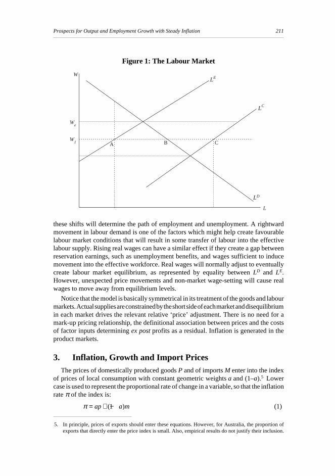
The demand for labour hours LD is given by its marginal product, and can be expressedin a form in which it depends on the level of output, the hourly real wage paid and therate of labour-augmenting technical change. Because of problems associated withhysteresis, labour supply is not a straightforward concept. For some purposes it is thesupply of those working plus those seeking work, as measured by the labour forcestatistics. This is denoted by LC in Figure 1. Some of those seeking work are so lacking(or perceived to be lacking by employers) in required work skills that they have eitherlost (because of their unemployment history) or never acquired, that their supply forthese and other reasons does not put downward pressure on the real wage.3 They are notpart of ‘effective labour supply’ which is given by LE.4 Hence, while we observe pointson LC and LD, LE can only be estimated indirectly out of equilibrium. When the labourmarket is in equilibrium at the wage that equates LD and LC, the difference between LE

and LC measures the natural rate of unemployment.

With the wage W1 there is effective excess demand for labour of AB which will causewages to rise despite the existence of unemployment as measured by BC = LC–LD.Changes in output and population, as well as technical change and the history ofunemployment will shift the functions in Figure 1. Together with changes in real wages,

3. Other reasons include wage-fixing systems that have little or no relation to market forces, poverty trapsand other institutional factors affecting the reservation wage of the unemployed.

4. This curve would have horizontal sections where there are minimum wages, which would show up bothat low wage levels and higher levels if market forces are prevented from affecting real wages. To the extentthat they apply to subsectors of the workforce, they would appear as a lower slope of LE.


these shifts will determine the path of employment and unemployment. A rightwardmovement in labour demand is one of the factors which might help create favourablelabour market conditions that will result in some transfer of labour into the effectivelabour supply. Rising real wages can have a similar effect if they create a gap betweenreservation earnings, such as unemployment benefits, and wages sufficient to inducemovement into the effective workforce. Real wages will normally adjust to eventuallycreate labour market equilibrium, as represented by equality between LD and LE.However, unexpected price movements and non-market wage-setting will cause realwages to move away from equilibrium levels.

Notice that the model is basically symmetrical in its treatment of the goods and labourmarkets. Actual supplies are constrained by the short side of each market and disequilibriumin each market drives the relevant relative ‘price’ adjustment. There is no need for amark-up pricing relationship, the definitional association between prices and the costsof factor inputs determining ex post profits as a residual. Inflation is generated in theproduct markets.

3. Inflation, Growth and Import PricesThe prices of domestically produced goods P and of imports M enter into the index

of prices of local consumption with constant geometric weightsa and (1–a).5 Lowercase is used to represent the proportional rate of change in a variable, so that the inflationrate π of the index is:

π = + −ap a m( )1 (1)

Figure 1: The Labour Market

W

We

W1 A B C

L

LE

LC

LD

5. In principle, prices of exports should enter these equations. However, for Australia, the proportion ofexports that directly enter the price index is small. Also, empirical results do not justify their inclusion.


Domestic goods prices are supposed to adjust to excess demand x according to

p p p p xe− = − = ′ > =−1 ( ), 0, (0) 0ψ ψ ψ (2)

The expected price change pe is taken to be determined by the change in the previousperiod.6 Combining Equations (1) and (2):

π π π ψ− = = + −−1 ( ) (1 )∆ ∆a x a m (3)

We estimate the price equation in the form in Equation (3).7

Two issues must be faced before this can be done. The first arises because Australiafloated in 1983:Q4 and previously had pegged or heavily managed its exchange rate.Secondly, excess demand in the goods market is not directly observable, though there area number of measures that are used to approximate it. Consider the exchange ratequestion. Pegging to a single currency or a basket means that fluctuations in those pricesdetermined on world markets are liable to be transmitted to the local economy in a fairlydirect manner. Further, it will be difficult to prevent foreign monetary expansionresulting in domestic monetary expansion, except by the process of raising interest ratesand reducing activity to such an extent that financial capital inflow is discouraged. Bycontrast, with a floating rate, domestic monetary policy can be independent of foreignmonetary conditions. It could be that the exchange rate system may approximate thetheoretical notion of ‘exchange rate insulation’ and ensure that domestic inflation isindependent of an average of movements in the foreign-currency prices of traded goods.8

Hence, it is preferable to examine the generation of inflation either for a pegged or afloating rate system, but not across both.9 For these reasons we have concentrated ourempirical analysis on the period of floating from 1983:Q4.

There are a number of observable variables that could proxy for excess demand in theproduct market, the gap between actual and potential output being one of the morepopular. Potential output is also not directly measured and is often taken to be someaverage of output levels. One difficulty about this is to know over what period and phaseof cycles to take the average, though different approaches could be accepted or rejectedon the basis of their empirical performance. Instead we have chosen to work with the rateof economic growth as the excess-demand proxy.10 Apart from the empirical results thisyields, there are some good theoretical reasons for this choice. We have also estimated

6. There is no survey information available for Australia on the expectations of those who set prices.

7. Strictly, the m in Equations (1) and (3) are different variables, the first being the import component of theCPI (for which there is no adequate data) and the second, the import price deflator from the NationalAccounts.

8. It is, of course, not possible to insulate against relative price movements of goods whose prices aredetermined on world markets. See Pitchford (1993) and the references therein.

9. An alternative would be to incorporate into the equation(s) those variables, such as the behaviour ofreserves, which distinguish a pegged from a floating system.

10. Snooks (1998) and in earlier works argues that inflation is a necessary concomitant of growth. Heinvestigates this in a very long-run historical context and with recent data for various OECD countries.Apart from the generation of inflation by growth, our approach differs from his in that we also allow forthe effect of prices of imports and for expectational effects that feed back on inflation.


an inflation equation using an output gap approach. The results, although similar, werenot superior to those with growth as the proxy.

The most compelling reason for relating inflation to real growth is that the growth ofthe labour force and capital stock, in conjunction with technical change, will at any timedetermine an underlying growth rate of ‘potential’ output. In the absence of largeexogenous shocks and cycles, this growth rate would probably remain relativelyconstant. If the supply potential from this growth were matched by demand growth at thesame rate, there would not be pressure for prices to rise. When the growth of demandexceeds that of supply, price signals will be required so that the intensity of use of factorscan be increased.11

There are arithmetical relationships between the growth rate of actual and potentialoutput and the divergence of output from some average level. To see this, define thegrowth rate g and excess demand x as:

gy y

yx

y y

y= − = −−

−

1

1

,˜

˜ (4)

where y is potential and y actual output. Then:

y

y

y

y

y

y

y

y−

−

− −=

1

1

1 1˜

˜ ˜

˜ , so that (5)

11

1(1 ˜) or 1

1

1 ˜(1 )

11+ = +

++ + = +

++

−−g

x

xg x

g

gx (6)

The growth rate is positively related to this period’s excess demand and the growth

rate of potential output g and negatively related to last period’s excess demand. Further,rewriting Equation (6) for time period -1, and by repeated substitution into Equation (6),taking logs, and using the approximation ln(1+z) ≅ z, this relation can be written:

(7)

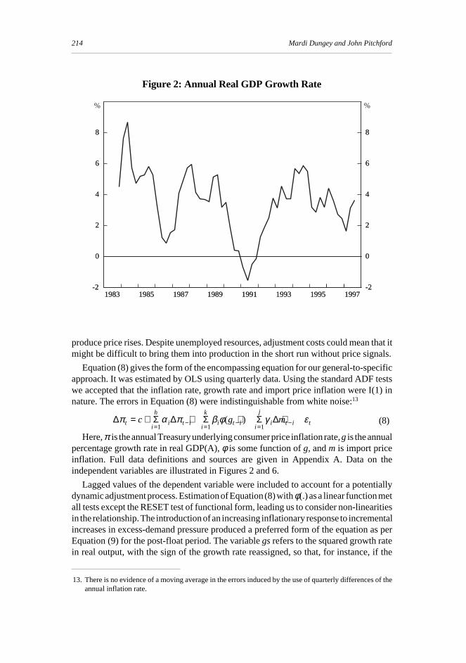
where µ(g) is the mean of g t− in the interval [-T, -1]. If these means are sufficiently closeto the growth rate of potential output, g will be a good approximation to excess demandplus a constant.12 Figure 2 shows the behaviour of g.

Another check can be made of our choice of growth as an excess demand proxy byregressing a measure of the output gap on growth. Some details are given in Appendix Cfrom which it can be seen that the two series are highly correlated.

Growth can also proxy for adjustment costs that are dependent on changes in the levelof, and/or growth rate of, output. For instance, suppose the economy is just leaving arecession, but output is still well below levels that would denote a boom. Although theeconomy is relatively depressed, a high growth rate at this time could nevertheless still

11. From this account of potential output, it could vary over the cycle. However, our procedures estimate anaverage and we do not attempt to measure its cyclical movement.

12. If potential output were defined as µ(g) they would differ only by the initial value of x and g .

x g g T g g x T= − + −{ } + − −˜ ( ) ˜ 1µ


produce price rises. Despite unemployed resources, adjustment costs could mean that itmight be difficult to bring them into production in the short run without price signals.

Equation (8) gives the form of the encompassing equation for our general-to-specificapproach. It was estimated by OLS using quarterly data. Using the standard ADF testswe accepted that the inflation rate, growth rate and import price inflation were I(1) innature. The errors in Equation (8) were indistinguishable from white noise:13

∆ Σ ∆ Σ Σ ∆π α π β φ γ εti

h

i t ii

k

i t ii

j

i t i tc g m= + + + += − = − = −

1 1 1( ) (8)

Here, π is the annual Treasury underlying consumer price inflation rate, g is the annualpercentage growth rate in real GDP(A), φ is some function of g, and m is import priceinflation. Full data definitions and sources are given in Appendix A. Data on theindependent variables are illustrated in Figures 2 and 6.

Lagged values of the dependent variable were included to account for a potentiallydynamic adjustment process. Estimation of Equation (8) with φ(.) as a linear function metall tests except the RESET test of functional form, leading us to consider non-linearitiesin the relationship. The introduction of an increasing inflationary response to incrementalincreases in excess-demand pressure produced a preferred form of the equation as perEquation (9) for the post-float period. The variable gs refers to the squared growth ratein real output, with the sign of the growth rate reassigned, so that, for instance, if the

Figure 2: Annual Real GDP Growth Rate

1983 1985 1987 1989 1991 1993 1995 19971983 1985 1987 1989 1991 1993 1995 1997-2

0

2

4

6

8

-2

0

2

4

6

8

-2

0

2

4

6

8

-2

0

2

4

6

8

% %

13. There is no evidence of a moving average in the errors induced by the use of quarterly differences of theannual inflation rate.


annual growth rate in one quarter was -2 per cent then gs for that quarter would be-4 per cent. Further details are available in Pitchford and Dungey (1998).

∆ ∆ Σ Σ ∆π α π β γ εt ti

i t ii

i t i tc gs m= + + + +− = − = −1 11

3

1

3(9)

In the final analysis we could not reject the hypothesis that the coefficients on the firstand second lags of gs were of equal value and opposite sign. After imposing this as arestriction, the change in the inflation rate was related positively and equally to both thechange in the ‘square’ of the growth rate (lagged once) and the ‘square’ of the growth rateitself (lagged 3 times).14 The estimated equation is shown in Equation (10), with standarderrors given in parentheses. Recursive estimation indicated that these parameter estimateswere stable over the estimation period.

(10)

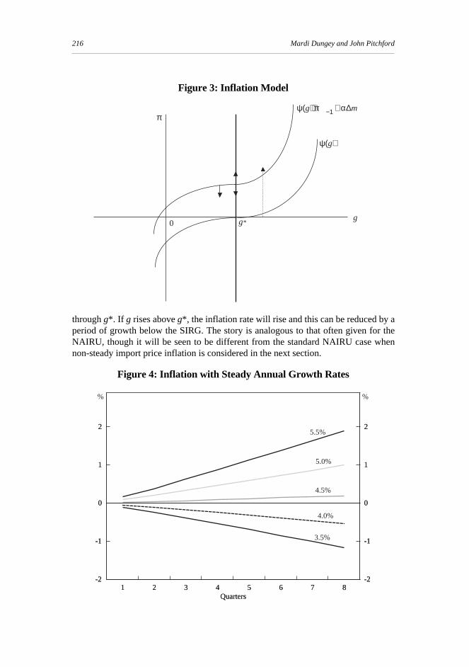
The lagged value of the inflation rate was significant, suggesting that not all of theadjustment of the domestic inflation rate implied by Equation (8) is completed in eachperiod.15 The functional form relating growth to inflation change is illustrated inFigure 3 where ψ φ ψ( ) ( ) * and ( *) 0.g g g g= − =

3.1 The influence of growth on inflation

The models enable an estimate to be made of the growth rate of GDP compatible withsteady inflation, or SIRG. If both the index of inflation and the rate of import priceinflation are constant, then from Equation (8),

(11)

Calculating the SIRG g* from gs*, for the data period of the float from December 1983it is 4.37 per cent per annum.

Figure 3 illustrates how the system works. Suppose, initially, that ∆m = 0. Thefunction ψ(g) represents inflation outcomes when the expected inflation rate is zero.Plotted against the inflation rate, it is positively sloped except at g* where it intersectsthe g-axis. If growth is at g*, the inflation rate can lie anywhere along the vertical axis

14. The restriction that the coefficients on ∆gst-1

and gst-3

were equal could not be rejected. This was tested inthe original equation with the equivalent test that the coefficients β

i in Equation (9) were equal, thus

preserving correct size in the test.

15. It is sometimes claimed that expectational effects are asymmetrical in that, for instance, reducing inflationrequires more foregone growth than the extra growth required to raise inflation. Hence we looked forasymmetrical responses of inflation by including the signs of independent variables in the regressions, butthe results were insignificant. Another matter examined was whether the stage of the cycle (e.g. time sincethe trough) might affect the degree of responsiveness to the growth rate, but the results did not support thiseither.

∆ ∆ ∆

∆ ∆ ∆

π πt t t t

t t t

gs gs

m m m

= − + + +

+ + +

− − −

− − −

0.2 0.36 0.015 0.015

(0.06 ) (0.0 ) (0.004) (0.003)

0.030 . .

(0.007) (0.008) (0.008)

1 3

1

79 0

4 88

0 023 0 030

1

2 3

gs c ii

k* = − = ∑

=β β β

1


Figure 3: Inflation Model

Figure 4: Inflation with Steady Annual Growth Rates

gg*

π

0

ψ(g)

ψ(g) + π−1 + α∆m

1 2 3 4 5 6 7 81 2 3 4 5 6 7 8-2

-1

0

1

2

-2

-1

0

1

2

-2

-1

0

1

2

-2

-1

0

1

2

QuartersQuarters

5.5%

% %

5.0%

4.5%

4.0%

3.5%

through g*. If g rises above g*, the inflation rate will rise and this can be reduced by aperiod of growth below the SIRG. The story is analogous to that often given for theNAIRU, though it will be seen to be different from the standard NAIRU case whennon-steady import price inflation is considered in the next section.


To appreciate the magnitude of the effect of growth on inflation implied by thecoefficients given in Equation (10), consider the consequences of a sustained rise or fallin g when the system has been at the SIRG for a long period, illustrated in Figure 4.Starting from a steady state with zero inflation, and then setting a steady GDP growth rateof 5.5 per cent per annum will mean that the system will reach about 1 per cent annualinflation after one year, and 2 per cent after two years. By comparison, with a 5 per centreal growth rate, inflation will take twice as long to reach 1 per cent per annum. Aftertwo years, with 4 per cent GDP growth, annual deflation of about 0.5 per cent per annumwill have been attained. All this assumes that import prices are not contributing toinflation.

3.2 Import prices

Growth and hence employment are affected by policy toward inflation. We haveshown that a steady inflation rate for domestic goods can be achieved by setting thegrowth rate at the SIRG. On the other hand, import prices fluctuate considerably(Figure 6) so that stabilising the overall inflation rate could require large oscillations ingrowth and hence in unemployment. Here we argue that it is critical to distinguishbetween, and adopt different policies toward, these two sources of inflation.

According to the ‘law of one price’, a behavioural relationship, arbitrage will ensurethat:

HM M* = (12)

where H is the nominal exchange rate (the reciprocal of the TWI), M* the foreigncurrency price of imports, and M the price in domestic currency. For the post-float period,a simple regression of m on h yields a correlation coefficient of 84 per cent and of h onthe inflation rate of the price index (π), a correlation coefficient of 6.3 per cent.Domestic-currency import price inflation is closely associated with nominal exchangerate variations. But nominal exchange rate variations are much larger than those in thedomestic inflation rate. Hence, there is a priori evidence that domestic-currency importprices are more closely related to exchange rate changes than to domestic conditions, anddomestic inflation and exchange rate movements are quite dissimilar.16

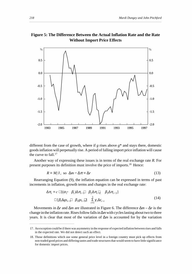
Import prices enter into the results in the way predicted by Equation (3) with lags ofone, two and three periods. One way of appreciating their influence is to ask whatinflation would have been if import prices had contributed to inflation to the same extentas domestic goods prices. This can be determined by substituting π for m inEquation (10) and calculating the consequent inflation from a base date, December 1983.The results are summarised in Figure 5 from which it can be seen that import priceinflation held down the overall inflation rate by between one and two percentage pointssince 1987. Depreciation in the mid 1980s added to inflation, but from about 1987, thecontribution of import prices has been steadily negative. Anti-inflation policy hasbenefited considerably from these import price movements.

If import price inflation rises, the curve ψ(g) rises (Figure 3), but it keeps moving uponly if import price inflation continues to increase. It is important to note that this is

16. For the pre-float period (1972–83), the correlation coefficient for the regression of m on h is 16 per cent.


different from the case of growth, where if g rises above g* and stays there, domesticgoods inflation will perpetually rise. A period of falling import price inflation will causethe curve to fall.17

Another way of expressing these issues is in terms of the real exchange rate R. Forpresent purposes its definition must involve the price of imports.18 Hence:

R M I m r= − =, so ∆ ∆ ∆π (13)

Rearranging Equation (9), the inflation equation can be expressed in terms of pastincrements in inflation, growth terms and changes in the real exchange rate:

(14)

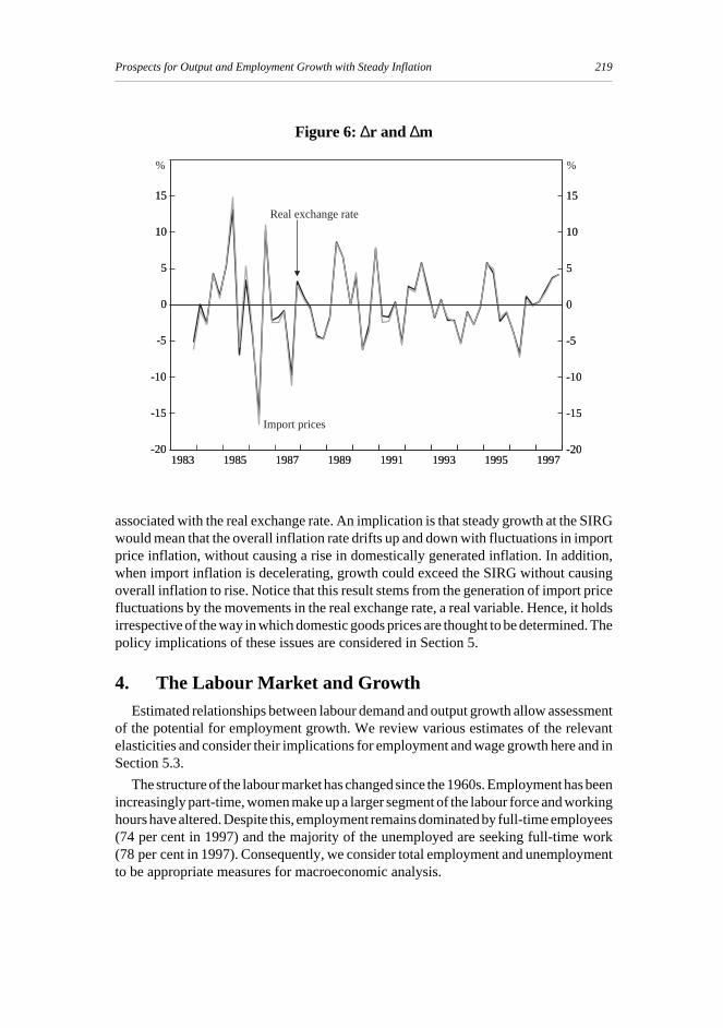
Movements in ∆r and ∆m are illustrated in Figure 6. The difference ∆m – ∆r is thechange in the inflation rate. Rises follow falls in ∆m with cycles lasting about two to threeyears. It is clear that most of the variation of ∆m is accounted for by the variation

Figure 5: The Difference Between the Actual Inflation Rate and the RateWithout Import Price Effects

1983 1985 1987 1989 1991 1993 1995 19971983 1985 1987 1989 1991 1993 1995 1997-2.0

-1.5

-1.0

-0.5

0.0

0.5

-2.0

-1.5

-1.0

-0.5

0.0

0.5

-2.0

-1.5

-1.0

-0.5

0.0

0.5

-2.0

-1.5

-1.0

-0.5

0.0

0.5

% %

17. An exception could be if there was asymmetry in the response of expected inflation between rises and fallsin the expected rate. We did not detect such an effect.

18. Those definitions which use some general price level in a foreign country must pick up effects fromnon-traded good prices and differing tastes and trade structures that would seem to have little significancefor domestic import prices.

∆ ∆ ∆ ∆

∆ Σ ∆

π α β π β π β π

β β γ

t t t t

t ti

i t i

c

gs gs r

= + − + +

+ + +

− − −

− − = −

[( ) ]

[ ]

1 1 1 2 2 3 3

1 1 3 31

3


associated with the real exchange rate. An implication is that steady growth at the SIRGwould mean that the overall inflation rate drifts up and down with fluctuations in importprice inflation, without causing a rise in domestically generated inflation. In addition,when import inflation is decelerating, growth could exceed the SIRG without causingoverall inflation to rise. Notice that this result stems from the generation of import pricefluctuations by the movements in the real exchange rate, a real variable. Hence, it holdsirrespective of the way in which domestic goods prices are thought to be determined. Thepolicy implications of these issues are considered in Section 5.

4. The Labour Market and GrowthEstimated relationships between labour demand and output growth allow assessment

of the potential for employment growth. We review various estimates of the relevantelasticities and consider their implications for employment and wage growth here and inSection 5.3.

The structure of the labour market has changed since the 1960s. Employment has beenincreasingly part-time, women make up a larger segment of the labour force and workinghours have altered. Despite this, employment remains dominated by full-time employees(74 per cent in 1997) and the majority of the unemployed are seeking full-time work(78 per cent in 1997). Consequently, we consider total employment and unemploymentto be appropriate measures for macroeconomic analysis.

Figure 6: ∆r and ∆m

1983 1985 1987 1989 1991 1993 1995 19971983 1985 1987 1989 1991 1993 1995 1997-20

-15

-10

-5

0

5

10

15

-20

-15

-10

-5

0

5

10

15

-20

-15

-10

-5

0

5

10

15

-20

-15

-10

-5

0

5

10

15

% %

Real exchange rate

Import prices


Labour demand is normally derived using a production function to relate real wagesto the marginal product of labour.19 Consider an aggregate CES production functionrelating capital (K) and labour (N) in the production of output Y:

Y t K t N= +− − −[ ( ) ( ) ]

1

γ µβ β α (15)

where β /α is the degree of returns to scale. The elasticity of substitution is found from:

wY

NN Y= = − + +∂

∂βα

µ β α( 1) ( 1) (16)

rY

KK Y= = − + +∂

∂βα

γ β α( 1) ( 1) so that (17)

ln lnw

r

N

K= − +

µγ

β( 1) (18)

It follows that the elasticity of substitution σ is 1/(1+β).

Equation (18) is a labour demand function relating N to time (through µ (t)), w and Y.Writing it in logarithmic form:

ln ln ln ln lnN t Y w= + + ++

−σ β α σ µ αβ

σ( / ) ( )1

1(19)

which in the constant returns to scale case reduces to:

ln ln ln lnN t Y w= + −σ µ σ( ) (20)

Supposing µ(t)=eξt, in the general case:

ln ln ln lnN t Y w= + + ++

−σ β α σξ αβ

σ( / )1

1(21)

The (semi-) elasticities with respect to time, output and real wages, respectively, areσm, (α+1)/(β +1), and σ. In the constant returns to scale case they are σξ, 1, and σ, andthe constant is zero.

Various estimations of this form of labour demand equations have been carried out forAustralian data and internationally. There are many disadvantages to such a system, themost striking being the identification problem. However, in the spirit of Hamermesh (1993)we consider that naive labour demand equations of this type have some merit as abenchmark for more sophisticated analysis.20

In Dungey and Pitchford (1998) we estimate a naive labour demand curve inerror-correction model (ecm) form for a number of market segments and measures oflabour and real wages. Here we report only the results of demand for labour in persons.The use of employed persons, rather than hours, raises the question of potential

19. See, for example, Hamermesh (1993).

20. The economy would have operated on the labour demand curve if the period considered could becharacterised as one of excess supply of labour. However, our theoretical analysis implies that this cannotbe inferred without knowing the effective supply curve.


substitution between employees and working hours. Firms may choose to pay more forextra hours from existing employees rather than hire more bodies (Hamermesh 1993),and they may choose to hire extra persons on a part-time basis. The Australian labourmarket has changed over the past two decades, in particular it has become increasinglyflexible. One consequence is that additional persons employed may not accurately reflectchanges in the hours of labour demanded. In an attempt to account for the changing hoursof work, we augment the traditional labour demand equation with an hours-workedvariable as per the TRYM model of the Australian economy (CommonwealthTreasury 1996). The form of the estimated equation in Dungey and Pitchford (1998) forall employees over the period 1984:Q4 to 1997:Q1 is:

∆ ∆ ∆e t e q y wt t t t t t= + + + + + +− −α α α α δ δ ε0 1 2 1 1 1 23 (22)

where e is total employment, t is a trend variable and q is a vector of independent variablescomprising real output y, given by GDP(A); real wages w, represented by real earnings;and average weekly hours, hr. ε is a random error term. The variables are in logarithmicform and full data descriptions and sources are contained in Appendix A. Further detailsregarding the estimation of Equation (22) are contained in Appendix B. The followingresults were obtained:

∆

∆ ∆

e t e y w

hr y w

t t t t

t t t

= − − − + −

− + −

− − −

−

1 022 06 397 2

76 4 72 42

0 251 0 138

098 77

. 0.0014 0.3 0. 0.12

(0.4 ) (0.0003) (0.06 ) (0.0 ) (0.0 )

0.015 . .

(0.098) (0. ) (0.0 )

1 1 1

1 (23)

In both our estimates and the existing Australian empirical literature, the form of thelong-run relationship in the estimating equations can be characterised as in Equation (24):

e t y w zt t t t= + + + +γ γ γ γ η0 1 2 3 (24)

where z is a vector of independent variables and η is the corresponding vector ofcoefficients.

In this section we are interested in the long-run elasticity parameters γ2 and γ3 and thetechnological change parameter γ1. Our output elasticity is a little higher and wageelasticity somewhat lower than the findings of earlier researchers, but are consistent withthose of Debelle and Vickery (1998). As they note, part of this effect is due to the choiceof data and time period.

Estimation of Equation (22) over a longer time period suggests similar wageelasticities, and the standard Chow tests do not indicate breaks in the relationship.However, recursive estimations indicate that the regressions had difficulty in fitting thedata in the early 1980s, in a period where employment growth continued despite highwage growth (Gregory 1986; Crosby and Olekalns 1998) suggesting there is a case fordistinguishing the recent labour market experience from earlier evidence. Russell andTease (1991) estimate the long-run wage elasticity at 0.67 for full-time male employeesusing real unit labour costs as the measure of wages for the period 1969–87.21 The

21. Russell and Tease modify the unit labour cost series by using smoothed GDP in its construction. We canobtain similar results to theirs using the unit labour cost data. However, the data needed for a study ofemployment should be per head of employees, not per unit of output.


TRYM model obtains an elasticity of substitution of 0.78 after making adjustment for theimpact of vacancies over the business cycle for 1971 to 1995 (without this adjustmentthe reported wage elasticity is calculated at -0.32). Table 1 gives the values of γi from theTRYM model (Commonwealth Treasury 1996), Russell and Tease (1991) and ourestimates.

Under the assumption of no change in the zt variables, the relationship in Equation (25)enables consideration of consistent scenarios of employment, output and real wagesgrowth using long run elasticities:

∆ ∆ ∆ ∆e y w zt t t t= + + +γ γ γ η1 2 3 (25)

Using the parameters in Table 1, we produce a set of ‘scenario’ charts to illustrate theconsequences of long-run elasticities. Consider first the naive estimates from Dungeyand Pitchford.

Table 1: Long-run Parameters

Study Technical change (γ1) Output elasticity (γ2) Wage elasticity (γ3)

Dungey and Pitchford -0.005 1.30 -0.40

TRYM -0.008 0.91 -0.79

Russell and Tease -0.0005 0.67 -0.61

Figure 7 shows bands of real wage growth consistent with output and employmentgrowth in the economy. According to the naive parameters, if real output in the economyis growing at 3.5 per cent, then employment growth of between 0.5 per cent and1 per cent per annum is consistent with real wage growth in the 4–6 per cent band.22 Asthe real output growth rate increases and the rate of employment growth falls (a moveright and down in the graph) the consistent real wage growth rate rises. At higher (lower)output growth and lower (higher) employment growth, the consistent real wage growthrises (falls).

For the parameter estimates from TRYM and taking the case of 3.5 per cent real outputgrowth, falling employment growth is associated with positive real wage growth(Figure 8). For the Russell and Tease estimates, 3.5 per cent output growth is consistentwith positive employment growth when real wage growth is less than 4 per centper annum. The Russell and Tease scenarios (not shown here) indicate higher real wagegrowth rates consistent with falling employment (through growth below the SIRG) thando the TRYM model scenarios, but lower real wage growth than our estimates.

It should be borne in mind that these elasticities are ‘long run’ constructs so that theiruse to illustrate short-run scenarios may be inappropriate. In Section 5 we use theadjustment equation from which these elasticities are derived, in conjunction withfurther assumptions about wage and GDP growth rates, to construct several prospects forunemployment.

22. A consistent real wage growth rate can be calculated more accurately, for example at 5.6 per cent for a0.5 per cent rise in employment, but is less useful for analytical purposes.


Figure 7: Pitchford and Dungey Growth Scenarios: Growth in RealOutput, Employment and Real Earnings

Real earnings growth is shown in 2 per cent bands

Figure 8: TRYM Growth Scenarios: Growth in Real Output,Employment and Real Earnings

Real earnings growth is shown in 2 per cent bands

-0.5

0.0

0.5

1.0

1.5

2.5 3.0 3.5 4.0 4.5

2% to 4%

Real output

Em

ploy

men

t

6% to 8%

10% to 12%

-0.5

0.0

0.5

1.0

1.5

2.5 3.0 3.5 4.0 4.5

-4% to -2%

Real output

Em

ploy

men

t

-2% to0%

0% to 2%


5. Policy IssuesThe results in preceding sections suggest ways of achieving higher growth of

employment and output consistent with steady inflation. These are discussed under theheadings of sources of inflation, the SIRG, and real wages and unemployment.

5.1 Sources of inflation

Attempting to manage inflation without reference to its source is likely to lead toconsiderable fluctuations in growth. In particular, inflation arising from domestic excessdemand should be distinguished from inflation due to import price movements as theyhave been shown to have different types of behaviour, a point also made by Stevens (1992).Thus, if the equilibrium growth rate is exceeded, domestic inflation will start to rise. Theoptions will then be either a period of growth below the SIRG or the prospect of theeventual establishment of a permanently higher inflation rate at the SIRG. On the otherhand, while rising inflation of imported goods can cause the overall inflation rate to rise,a subsequent fall in this source of inflation will bring the inflation rate down again,without the necessity for departing from the SIRG. Movements in the real exchange rate(defined as the ratio of the import price deflator to the underlying consumer price index),are the major source of fluctuations in this category of inflation (Figure 9). The factorsinfluencing it include monetary and fiscal disturbances, movements in the IS andLM curves, shifts in currency preferences and changes in the terms of trade.

It can be seen from the rate of change part of Figure 9 that the real exchange ratefluctuates widely and regularly. Also the index shows that there have been long periodsof appreciation and depreciation, depreciating in the mid 1980s, appreciating in the late1980s and through 1984 to 1987. How should policy respond to the effects on inflationof such real exchange rate movements? Earlier we noted the benefit that the recent realappreciation provided for inflation control in the 1990s, but what about depreciation?Suppose the economy is at some target positive inflation rate. Real depreciation meansthat the prices of imports rise relative to those of domestic goods. In order for monetarypolicy to maintain inflation at a particular rate, GDP growth would be required to fall.In the face of real exchange rate changes there would seem to be a strong case formaintaining the SIRG while letting inflation fluctuate. From Figure 5, it can be seen thatthe large depreciation in the mid 1980s significantly increased the inflation rate, butsubsequently this was more than offset by the large appreciation through to the end ofthe decade. Real appreciation continued to reduce the pressure on inflation through to1997.

If a real depreciation is allowed to raise inflation it could also have an effect onnominal and real wages and so on unemployment. Theoretical analysis does not giveunambiguous results about the impact of relative price shifts on real wages, the outcomeusually depending on factor intensities in different sectors.23 Leaving this aside, thereaction of the authorities in the case of the mid 1980s depreciation was to attempt to

23. See Stolper and Samuelson (1941), Meade and Russell (1957) and Pitchford (1963) for analyses of this,the latter papers establishing that almost anything can happen.


calculate the effects of depreciation on inflation and argue that nominal wages should notbe raised by that factor. This seems preferable to reducing real growth. Such policiesshould be increasingly unnecessary as wages become more market determined.

Although domestic macroeconomic policy can influence the real exchange rate tosome extent, it is probably fair to say that very large shifts in interest rates would beneeded to offset its changes and that much of its movement due to foreign sources isoutside such control. Hence, it would seem undesirable to attempt to control it, unlessdoing so accorded with some other objective. As a consequence, modest rates of inflationgenerated by import prices need not give rise to policy responses.

Data on inflation, import prices and GDP are available to policy-makers only after aconsiderable delay. However, the association between import price inflation and theTWI is sufficiently strong that its quarterly and monthly movements can provide someearly indication of the import price component’s effect on inflation, which could assistthe process of distinguishing the two sources of inflation. This is discussed further inAppendix C.

5.2 The SIRG

Policy toward inflation consists of two parts. The first involves choosing a desiredinflation rate, which in Australia takes the form of a target average rate falling in the bandof 2–3 per cent per annum. The second is achieving the band, which in a stochastic sensecan be thought of as attaining steady inflation at the desired rate. In such an equilibrium,growth would be at the SIRG and inflation could fluctuate with real exchange ratemovements.

Figure 9: Real Exchange Rate

0.8

1.0

1.2

0.8

1.0

1.2

0.8

1.0

1.2

0.8

1.0

1.2

-20

-10

0

10

-20

-10

0

10

-20

-10

0

10

-20

-10

0

10

%

Annual percentage rate of change

1989/90=1

%

1989/90=1

199719941991198819851982197919761973


When the domestic goods component of the inflation rate is rising or falling, someprocedure for adjusting interest rates is needed to bring the system to steady inflation. Aproblem with rules which target only overall inflation is that they do not distinguishbetween inflation arising from import prices and that originating in domestic goodsmarkets. Following such a rule with respect to the inflation index would lead growth tofluctuate when the real exchange rate fluctuated. Moreover, if there is evidence thatsuggests the existence of a growth rate consistent with steady inflation in the domesticcomponent, it would seem appropriate to use it. If growth is less (greater) than the SIRG,our analysis suggests that whatever rule operates, growth should be increased (reduced).24

Further, it would be prudent to watch inflation, both from domestic sources and fromimport prices and to react to their movements. Another consideration is that because ofpossible shifts through time, the use of the SIRG to guide policy would need to be handledwith care. Of course, this also applies to all policy indicators.

A possibility for a period of growth above the SIRG could arise when the contributionof real exchange rate movements to inflation is negative. This could particularly be thecase when a program to reduce unemployment is current. It might be feasible at suchtimes to edge growth up without raising the inflation rate. However, it would then beimportant to bear in mind that the effect of higher growth on inflation may come with alag of close to six months, allowing for the delay in data availability. The situation wouldneed to be appraised on the basis of the facts available at the time.

It might be thought that a conservative policy approach to inflation would be to keepgrowth below the SIRG. However, if this were done, and taking the case of a neutralimpact from import prices, the inflation rate will fall. If there is a cycle in growth,inflation will fall on average. Low inflation rates pose a problem for monetary policybecause the floor to nominal interest rates may not allow real interest rates to be set lowenough to help revive the economy from recession. Hence, some target positive averageinflation rate over a cycle will not be met unless growth exceeds the SIRG in a boom aswell as falling below it in the trough.

5.3 Real wages, growth and unemployment

Employment elasticity estimates can be used to give an answer to the question of theeffect of changes in the non-market component of wages on employment.25 Instead ofaddressing this issue, we use the elasticities from Section 4 to examine variouspossibilities for reducing unemployment through higher growth. To do this it isnecessary to make assumptions about the behaviour of real wages and output. Table 2provides a way of looking at their association through time. Even the period 1972:Q3 to1983:Q3, which includes the large real wage increases in the seventies and early eighties,did not result in average real wage growth exceeding that of real GDP.

This experience suggests two potentially interesting cases, that is where wages andGDP grow at similar rates as in the first subperiod, and where wage growth is about half

24. The Taylor rule involves adjustment to both output and inflation, so could be extended to a growth target.It would also need modification so that it distinguished between sources of inflation.

25. This exercise is undertaken by Debelle and Vickery (1998).


that of GDP as in the third column of the table.26 We assume that labour force growthis 1.25 per cent per annum which is near its current average.27 This is probably anoptimistic assumption as the participation rate could well rise with falling unemploymentand rising wages. Initial values for the variables in the short-run adjustment equation aretaken at their 1997:Q4 levels, including an unemployment rate of 8.4 per cent.28 Theshort-run scenario results are sensitive to the initial values as they involve levelsvariables.

Table 2: Mean Annual Growth Rates of Real GDP and Real Earnings

Mean growth 1972:Q3 – 1983:Q3 – 1992:Q3 – 1972:Q3 –1983:Q3 1989:Q3 1997:Q4 1997:Q4

Real GDP 2.7 4.4 3.8 3.17

Real earnings 2.3 -1.0 2.1 1.36

The following scenarios are, of course, meant only to be indicative of possible resultsand are in no way predictions. After reviewing them we shall look at ways in whichchanges in our assumptions might affect their outcomes.

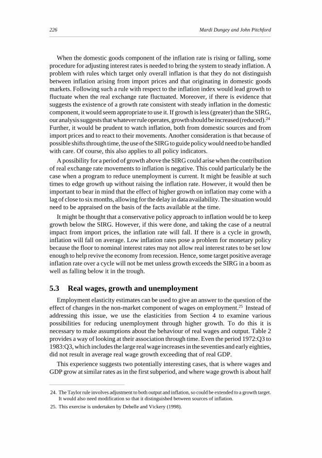
In scenario 1 shown in Figure 10, we assume that output growth is raised immediatelyto the SIRG and held there. In the case in which wage growth is half output growth, byMarch 2000 unemployment would be down to 7.4 per cent and by December 2002 to4.9 per cent. Inflation would fall to, and stay around, 1 per cent per annum. Bycomparison, if output growth is initially raised to 5.5 per cent, but then brought back to5 per cent after one year and to the SIRG after two years, inflation will rise, but remainin the 2–3 per cent band (Figure 11). Under the optimistic scenario (real wages grow athalf the rate of output), the unemployment rate falls to 7.2 per cent after two years and4.5 per cent after four. Note that the labour force and employment grow at rates that areapproximately constant, and that the shape of the curve in these scenarios is driven bythe rise in E/L, where the change in the unemployment rate, ∆u, is given by100∗{ E/L}( ∆l–∆e) and ∆l is growth in the labour force, L.

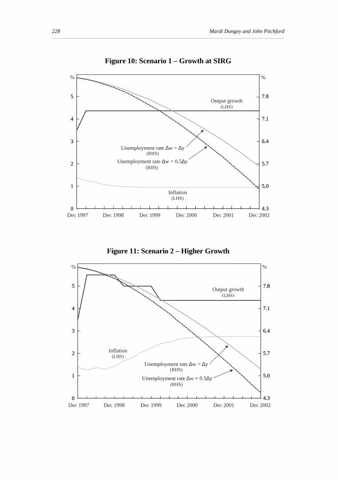
The final figure (12) compares unemployment paths using the optimistic wageassumption cases of scenarios 1 and 2, with the outcome arising from the 1998–99Budget growth assumption. We suppose this implies that growth is 3.5 per cent for thefirst quarter of 1998 and then 3 per cent until the end of 1999, thereafter reverting to theSIRG. The results are not particularly different in the first year, but leave the economywith half a percentage point more of unemployment, when compared with the highgrowth case, by the year 2000. A qualification to these outcomes is that the Asiancurrency crisis has led to a depreciation of the $A which will ensure that the overallinflation rate will be higher than we have calculated, given our neutral assumption aboutimport prices.

26. The Accord experience in the 1980s is unlikely to be repeated.

27. Other cases are examined in Dungey and Pitchford (1998).

28. These simulations use the employment equation in Appendix B and assume no change in averageweekly hours.


Figure 10: Scenario 1 – Growth at SIRG

0

1

2

3

4

5

4.3

5.0

5.7

6.4

7.1

7.8

0

1

2

3

4

5

4.3

5.0

5.7

6.4

7.1

7.8

% %

Unemployment rate ∆w = ∆y(RHS)

Unemployment rate ∆w = 0.5∆y(RHS)

Dec 2002Dec 2001Dec 2000Dec 1999Dec 1998Dec 1997

Inflation(LHS)

Output growth(LHS)

Figure 11: Scenario 2 – Higher Growth

0

1

2

3

4

5

4.3

5.0

5.7

6.4

7.1

7.8

0

1

2

3

4

5

4.3

5.0

5.7

6.4

7.1

7.8

% %

Inflation(LHS)

Unemployment rate ∆w = ∆y(RHS)

Unemployment rate ∆w = 0.5∆y(RHS)

Dec 2002Dec 2001Dec 2000Dec 1999Dec 1998Dec 1997

Output growth(LHS)


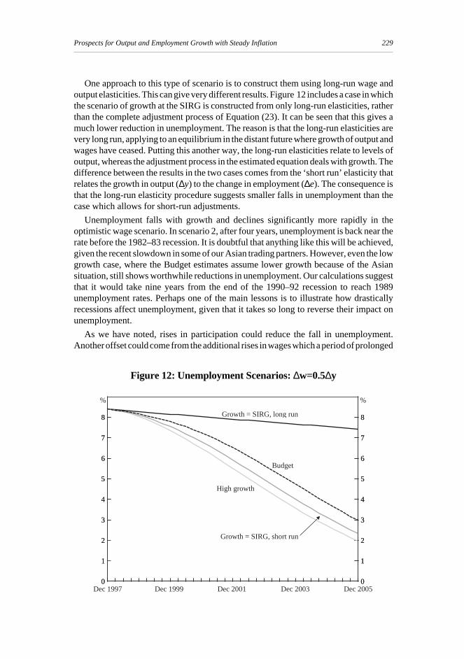
One approach to this type of scenario is to construct them using long-run wage andoutput elasticities. This can give very different results. Figure 12 includes a case in whichthe scenario of growth at the SIRG is constructed from only long-run elasticities, ratherthan the complete adjustment process of Equation (23). It can be seen that this gives amuch lower reduction in unemployment. The reason is that the long-run elasticities arevery long run, applying to an equilibrium in the distant future where growth of output andwages have ceased. Putting this another way, the long-run elasticities relate to levels ofoutput, whereas the adjustment process in the estimated equation deals with growth. Thedifference between the results in the two cases comes from the ‘short run’ elasticity thatrelates the growth in output (∆y) to the change in employment (∆e). The consequence isthat the long-run elasticity procedure suggests smaller falls in unemployment than thecase which allows for short-run adjustments.

Unemployment falls with growth and declines significantly more rapidly in theoptimistic wage scenario. In scenario 2, after four years, unemployment is back near therate before the 1982–83 recession. It is doubtful that anything like this will be achieved,given the recent slowdown in some of our Asian trading partners. However, even the lowgrowth case, where the Budget estimates assume lower growth because of the Asiansituation, still shows worthwhile reductions in unemployment. Our calculations suggestthat it would take nine years from the end of the 1990–92 recession to reach 1989unemployment rates. Perhaps one of the main lessons is to illustrate how drasticallyrecessions affect unemployment, given that it takes so long to reverse their impact onunemployment.

As we have noted, rises in participation could reduce the fall in unemployment.Another offset could come from the additional rises in wages which a period of prolonged

Figure 12: Unemployment Scenarios: ∆w=0.5∆y

% %

Growth = SIRG, long run

High growth

Budget

Growth = SIRG, short run

Dec 2005Dec 2003Dec 2001Dec 1999Dec 19970

1

2

3

4

5

6

7

8

0

1

2

3

4

5

6

7

8

0

1

2

3

4

5

6

7

8

0

1

2

3

4

5

6

7

8


growth could produce. Further, rising real wages may have a greater negative impact ongrowth than we have allowed for via the ‘scale effect’ when the economy is on the supplycurve.29 Our assumptions about the relationship between output and wage growthbecome less likely to hold, the further the system moves from the base date. Nevertheless,our results raise the possibility that higher growth could contribute significantly toreducing unemployment.

Other scenarios which make alternative assumptions about the behaviour of theworkforce could well show smaller reductions in unemployment, as it is likely that theparticipation rate would rise considerably during a long period of growth of output,wages and employment. These responses are one of the least understood facets of thelabour market.

6. Concluding RemarksLow unemployment was the norm for Australia during the thirty years following

World War 2. This is too long a period for ‘full employment’ to be dismissed as a transientor rare event, so it must remain a challenge for economists to find how to recover it. Atthe macroeconomic level, faster economic growth and less drastic recessions are themain ways of reducing unemployment. This is not a panacea, because higher growth willbring the potential for rising inflation. Our object has been to investigate the concept ofa GDP growth rate compatible with steady inflation, and we find an association betweengrowth and domestically generated inflation that is at least as robust empirically as manyalternative approaches. This is also supported by approaching the relationship indirectlythrough a version of the output gap concept and relating growth to the gap. Our figurefor the steady inflation rate of growth (SIRG) for the post-float period is 4.37 per centper annum.

Inflation also arises from fluctuations in import prices and this, as often as not, takesthe form of a negative impact. We argue that inflationary pressures from this sourceshould be absorbed by allowing the overall inflation rate to move up or down, rather thanby reducing growth below the SIRG. Some of Australia’s most severe inflationaryepisodes, such as the Korean wool-price boom and the oil price shocks, have come fromsuch external sources. The pegged exchange rate system of those times was not wellsuited to absorbing such shocks, but a floating rate system at least allows an independentmonetary policy.

If import price inflation is falling, there will be some scope for growth above the SIRGto help achieve falling unemployment without rising inflation. Further, if as seems verylikely, the economy continues to produce growth cycles there will be scope for highergrowth than the SIRG in the upswing. If this is not the case, there will be a tendency forthe average inflation rate to lie under the target band and even to fall so low that there isdifficulty in conducting effective monetary policy in times of recession.

Given the poor state of knowledge about the elasticities of demand for, and particularlysupply of, labour, there must be doubt as to the extent to which growth can contribute toreducing unemployment. However, our scenarios suggest that it might be possible to

29. See Debelle and Vickery (1998) for a discussion of the scale effect.


bring unemployment down to the vicinity of 1989 pre-recession rates over the next fourto five years if actual outcomes for growth and wages approximate those of our optimisticassumptions, or even those of some of our less optimistic cases. Historically, periods ofhigh activity and growth such as in World War 2 and during 1945–75 were accompaniedby low unemployment. It would be surprising if growth were not the cause of suchfavourable employment experience.

Macroeconomic measures to promote growth without rising inflation would no doubthave greater effect in more flexible labour markets. Nevertheless, it should not beforgotten that rigidity in labour markets characterised postwar Australia much more thanat present. Given that most microeconomic measures to reduce unemployment aim tocreate structural change, it is likely that they too would work better in an environmentof high growth.


Appendix A: Data DefinitionsE: Quarterly total non-farm employment taken from the NIF database on DX

[VNEQ.AN_NNE].

HR: Quarterly total average weekly hours (seasonally adjusted) from the NIF databaseon DX [VNEQ.AN_NHT].

M: Quarterly implicit price deflator for imports from the TSS database on DX[NPDQ.AD90IMP#].

p: Quarterly Treasury underlying Consumer Price Inflation rate taken from the TSSdatabase on DX [RSR.U190C9211001].

W: Quarterly real earnings index (seasonally adjusted) taken from the RBA databaseon DX [GLCREISA]. This series is constructed by the RBA taking total earningsfrom the national accounts to create a weekly earnings figure and then deflating bythe relevant consumption index (see the ‘Notes toTables’ to Table G.5 in theReserve Bank Bulletin).

X: The exchange rate – defined as the inverse of the trade-weighted index from theRBA database on DX [FXRTWI]. Quarterly data derived as the average of theend-month figures.

Y: Quarterly Australian real GDP(A) (seasonally adjusted) taken from the ABS TSSdatabase on DX [NPDQ.AK90GDP#A].

Capital letters denote data in levels and lower case denotes logged series.

Appendix B: Estimation Results

B.1 Inflation

(B1)

LM test for serial correlation0.968 RESET test 0.766

Normality (Jarque-Bera) 1.424 Heteroskedasticity 0.343

AIC = –12.4 SBC = –19.5 R 2 = 0.68Estimation period: 1983:Q4 – 1997:Q4

∆ ∆ ∆

∆ ∆ ∆

π πt t t t

t t t

gs gs

m m m

= − + + +

+ + +

− − −

− − −

0.2 0.3 0.01 0.0

(0.06 ) (0.0 ) (0.004) (0.003)

0.030 . .

(0.007) (0.008) (0.00 )

1 1 3

1

79 60 5 15

4 88

0 023 0 030

82 3


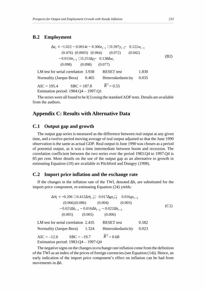
B.2 Employment

(B2)



AIC = 195.4 SBC = 187.8 R 2 = 0.55Estimation period: 1984:Q4 – 1997:Q1

The series were all found to be I(1) using the standard ADF tests. Details are availablefrom the authors.

Appendix C: Results with Alternative Data

C.1 Output gap and growth

The output gap series is measured as the difference between real output at any giventime, and a twelve-period moving average of real output adjusted so that the June 1990observation is the same as actual GDP. Real output in June 1990 was chosen as a periodof potential output, as it was a time intermediate between boom and recession. Thecorrelation coefficient between the two series over the period 1983:Q4 to 1997:Q4 is85 per cent. More details on the use of the output gap as an alternative to growth inestimating Equation (10) are available in Pitchford and Dungey (1998).

C.2 Import price inflation and the exchange rate

If the changes in the inflation rate of the TWI, denoted ∆h, are substituted for theimport price component, re-estimating Equation (24) yields:

(C1)



AIC = –12.6 SBC = –19.7 R 2 = 0.68Estimation period: 1983:Q4 – 1997:Q4

The negative signs on the changes in exchange rate inflation come from the definitionof the TWI as an index of the prices of foreign currencies (see Equation (14)). Hence, anearly indication of the import price component’s effect on inflation can be had frommovements in ∆h.

∆

∆ ∆

e t e y w

hr y w

t t t t

t t t

= − − − + −

− + −

− − −

−

1.02 0.0014 0.3 0. 0.12

(0.4 ) (0.0003) (0.06 ) (0.07 ) (0.04 )

0.015 . .

(0. ) (0. ) (0.0 )

2 06 397 2

76 4 2 2

0 251 0 138

098 098 77

1 1 1

1

∆ ∆ ∆

∆ ∆ ∆

π πt t t t

t t t

gs gs

h h h

= − + + +

− − −

− − −

− − −

0. 0.41 0.017 0.016

(0.0 )(0.0 ) (0.004) (0.003)

0.021 . .

(0.005) (0.0 5) (0.006)

1 1 3

1

296 2

66 86

0 016 0 022

02 3


ReferencesBarro, R. and H. Grossman (1976), Money, Employment and Inflation, Cambridge University

Press, Cambridge.

Commonwealth Treasury (1996), Documentation of the Treasury Macroeconomic (TRYM) Modelof the Australian Economy, CPN Printing, Canberra.

Crosby, M. and N. Olekalns (1998), ‘Inflation, Unemployment and the NAIRU in Australia’,Australian Economic Review, forthcoming.

Debelle, G. and J. Vickery (1998), ‘The Macroeconomics of Australian Unemployment’, paperpresented at this conference.

Dungey, M. and J. Pitchford (1998), ‘Employment, Growth and Real Wages in Australia’, mimeo,La Trobe University.

Gregory, R. (1986), ‘Wages Policy and Unemployment in Australia’, Economica, 53(210S),pp. S53–S74.

Hamermesh, D. (1993), Labor Demand, Princeton University Press, Princeton, New Jersey.

Malinvaud, E. (1977), The Theory of Unemployment Reconsidered, Basil Blackwell, Oxford.

Meade, J. and E. Russell (1957), ‘Wage Rates, the Cost of Living and the Balance of Payments’,Economic Record, 33(64), pp. 23–28.

Muellbauer, J. and R. Portes (1978), ‘Macroeconomic Models with Quantity Rationing’, EconomicJournal, 88(352), pp. 788–821.

Pitchford, J.D. (1963), ‘Real Wages, Money Wages and the Terms of Trade’, Economic Record,39(87), pp. 282–291.

Pitchford, J.D. (1993), ‘The Exchange Rate and Macroeconomic Policy in Australia’, inA. Blundell-Wignall (ed.), The Exchange Rate, International Trade and the Balance ofPayments, Reserve Bank of Australia, Sydney, pp. 147–201.

Pitchford, J.D. and M. Dungey (1998), ‘An Analysis of Inflation and Growth in Australia’, mimeo,Australian National University.

Russell, W. and W. Tease (1991), ‘Employment, Output and Real Wages’, Economic Record,67(196), pp. 34–45.

Snooks, G.D. (1998), Long Run Dynamics, Macmillan/St Martins Press, London and New York.

Stevens, G. (1992), ‘Inflation and Disinflation in Australia: 1950–91’, in A. Blundell-Wignall(ed.), Inflation, Disinflation and Monetary Policy, Reserve Bank of Australia, Sydney,pp. 182–244.

Stolper, S.F., and P.A. Samuelson (1941), ‘Protection and Real Wages’, Review of EconomicStudies, 9, pp. 58–73.

prospects for output and employment growth with … for output and employment ... of quantifying the...

Documents