proper analysis of the diallel mating design
TRANSCRIPT

Retrospective Theses and Dissertations Iowa State University Capstones, Theses andDissertations
1995
Proper analysis of the diallel mating designJay R. SughroueIowa State University
Follow this and additional works at: https://lib.dr.iastate.edu/rtd
Part of the Agricultural Science Commons, Agriculture Commons, Agronomy and CropSciences Commons, Biostatistics Commons, and the Genetics Commons
This Dissertation is brought to you for free and open access by the Iowa State University Capstones, Theses and Dissertations at Iowa State UniversityDigital Repository. It has been accepted for inclusion in Retrospective Theses and Dissertations by an authorized administrator of Iowa State UniversityDigital Repository. For more information, please contact [email protected].
Recommended CitationSughroue, Jay R., "Proper analysis of the diallel mating design " (1995). Retrospective Theses and Dissertations. 10987.https://lib.dr.iastate.edu/rtd/10987
INFORMATION TO USERS
This manuscript has been reproduced from the microfilm master. UMI filTTn; the text directly from the original or copy submitted. Thus, some thesis and dissertation copies are in typewriter face, while others may be from any type of computer printer.
The quality of this reproduction is dependent upon the quality of the copy submitted. Broken or indistinct print, colored or poor quality illustrations and photographs, print bleedthrough, substandard margins, and improper alignment can adversely affect reproduction.
In the unlikely event that the author did not send UMI a complete manuscript and there are missing pages, these will be noted. Also, if tmauthorized copyright material had to be removed, a note wiD indicate the deletion.
Oversize materials (e.g., maps, drawings, charts) are reproduced by sectioning the original, beginning at the upper left-hand comer and continmng from left to r^t in equal sections with small overlaps. Each original is also photographed in one exposure and is included in reduced form at the back of the book.
Photogr^hs included in the original manuscript have been reproduced xerographicaUy in this copy. Higher quality 6" x 9" black and white photographic prints are available for aity photographs or illustrations appearing in this copy for an additional charge. Contact UMI directly to order.
A Bell & Hciweli Information Company 300 North Zeeb Road. Ann Arbor. Ml 48106-1346 USA
313/761-4700 800/521-0600


Proper analysis of the diallel mating design
by
Jay R. Sughroue
A Dissertation Submitted to the
Graduate Faculty in Partial Fulfillment of the
Requirements for the Degree of
DOCTOR OF PHILOSOPHY
Department: Agronomy Major: Plant Breeding
Approved:
For the Ma]or Department
For the Graduate College
Iowa State University Ames, Iowa
1995
Signature was redacted for privacy.
Signature was redacted for privacy.
Signature was redacted for privacy.

UMI Number: 9540947
OMI Microform 9540947
Copyright 1995, by OMI Company. AH rights reserved.
This microform edition is protected against unauthorized
copying under Title 17, United States Code.
UMI 300 North Zeeb Road
Ann Arbor, MI 48103

ii
TABLE OF CONTENTS
Page
ACKNOWLEDGMENTS iii
GENERAL INTRODUCTION 1
Dissertation Organization 2
Literature Review 2
PROPER ANALYSIS AND INTERPRETATION OF THE DIALLEL MATING DESIGN 14
Abstract 14
Introduction 15
Material and Methods 18
Results 24
Discussion 28
References 34
GENERAL CONCLUSION 48
LITERATURE CITED 49
APPENDIX 51

iii
ACKNOVfLEDGMENTS
I would like to thank Dr. Arden Campbell, Dr. Charlie
Martinson, Dr, Paul Heiz, and Dr. Kendall Lamkey for serving
on my graduate study committee, A special thanks to Dr.
Kendall Lamkey for providing me with SAS programs and
assistance in analyzing the data in this study.
I would like to express my gratitude and appreciation to
everyone on the corn breeding project including graduate
students, visiting scientists, Paul White, and Mary Lents for
their help and friendship.
Dr, Arnel Hallauer, thank you for giving me the
opportunity to study under you. You taught me not only the
fundamentals of a good plant breeder but you instilled in me
that patience, hard work, and good relationships with other
team members are the keys to success. I will always cherish
the time we spent together in the field, lab, and class room.
Again, thank you for the guidance and inspiration you gave me.
To my parents and brother thank you for your belief and
support in my educational endeavors. To my wife Dilene, words
can not express my appreciation and love for all that you have
sacrificed and done to help me during my graduate studies.
Tyler, my son, thank you for your smiles and hugs after hard
days at school. You put it all into perspective.
1
GENERAL INTRODUCTION
The diallel mating design has been used successfully for
over 50 years in plant breeding to estimate the relative
combining ability of lines. From the diallel mating design,
plant breeders can estimate general combining ability (GCA)
and specific combining ability (SCA). Sprague and Tatum (1942)
defined GCA as "the average performance of a line in hybrid
combinations" and defined SCA as "those cases in which certain
combinations do relatively better or worse than would be
expected on the basis of the average performance of the lines
involved."
In the 1950s, however, the diallel mating design was
extended to estimate genetic variance components, and with
this use of diallel mating design came criticism, controversy,
and debate about its usefulness in supplying such information.
The controversy is centered around whether it is proper and
valid to estimate genetic variance components from parents of
a diallel that can not be considered to be a random sample of
a defined population. One of the assumptions required to
estimate genetic parameters using the diallel mating design is
that the genes in the parents must be independently
distributed.
Previous theoretical and computer simulation studies
found that the failure of this assumption often resulted in
the average level of dominance being overestimated (Hayman,

2
1954b; Nassar, 1965). The objective of this study was to test
the vglidlty of the assumption that the genes in the parents
of a diallel must be independently distributed.
Dissertation Organization
This dissertation is written in manuscript form and will
be submitted for publication in Crop Science. The paper is
preceded by a General Introduction section which includes a
Literature Review, and is followed by a General Conclusion
section. Literature cited in the General Introduction and
General Conclusion sections follows the General Conclusion
section. An Appendix section with additional analyses tables
is included at the end of this dissertation.
Literature Review
Plant breeders have several mating designs to select from
to investigate the genetic properties of plant populations,
but none of them has caused as much controversy and debate
than has the diallel mating design. According to Hallauer and
Miranda (1988) "The diallel mating design has been used and
abused more extensively than any other in maize and other
plant species." The diallel mating design is defined as making
all possible crosses among a group of genotypes. Sprague and
Tatum (1942) introduced the diallel cross concept to plant
breeding by making all possible crosses cimong a set of maize

3
{Zea mays L.) inbred lines. The diallel cross was first used
in animal breeding by Schmidt in 1919 when crosses were made
between two males and two females at different times (Lush,
1945). The term diallel cross as applied to plants, however,
did not appear in the literature until 1953 (Jinks and Hayman,
1953).
The theory and statistical analysis of the diallel mating
design have been investigated in depth by several researchers
(Jinks and Hayman, 1953; Hayman, 1954a, 1954b, 1958, 1960;
Griffing 1956a, 1956b; Kempthorne, 1956; Gardner and Eberhart,
1966; Eberhart and Gardner, 1966). Various forms of the
diallel crossing system and analysis have been developed since
its conception. Kempthorne and Curnow (1961) developed the
partial diallel as a way of increasing the number of parents
that could be used in a diallel. A partial diallel requires
fewer crosses per parent than does a regular diallel. Gardner
and Eberhart (1966) developed a model to investigate the
genetic properties of open-pollinated varieties and their
crosses.
Griffing (1956a) proposed four different methods of
analyzing a diallel based on whether the parents, their
reciprocal crosses, or both, are included in the evaluation
with the Fj crosses: (1) F^ crosses with parents and reciprocal
Fj crosses (n^); (2) F, crosses and parents [n(n+1)/2];(3) F^
crosses and reciprocal F^ crosses n(n-l); (4) F^ crosses only

4
[n(n-l)/2] (Griffing 1956a).
Hayman (1954a) proposed a method of analysis that
includes the parents, crosses, and the reciprocal
crosses. Jones (1965) later modified Hayman's model so that it
could be used without the reciprocal F^ crosses.
Gardner and Eberhart (1966) proposed three methods of
analyses. Analysis I is only for varieties and includes the
parent varieties, selfed progenies of the varieties, and the
variety crosses. Analysis II and Analysis III can be used with
either varieties or with homozygous lines» Analysis II
includes the parent varieties and the variety crosses while
Analysis III includes only the variety crosses-
From the proposed types of analyses of diallel crosses,
Griffing's methods two and four, Hayman's method, and Gardner
and Eberhart's Analyses II and III can be used to analyze the
same type of data. Sokol (1976; cited by Baker, 1978)
demonstrated that the statistical parameters of Griffing's
methods two and four, Hayman's method, and Gardner and
Eberhart's Analysis II are all linear functions of the
parameters in Gardner and Eberhart's Analysis III (1966).
The objective of this review is not to compare and
contrast the various proposed methods of analyses, since
previous authors have already reviewed them extensively
(Christie and Shattuck, 1992? Hallauer and Miranda, 1988).
Instead, the intent of this report is to review the basic

5
issues of the diallel mating design and to show the importance
of these issues to the plant breeder. Griffing's approach
(1956b) will be used primarily to illustrate these objectives
because it is the more widely used analysis among most plant
breeders.
Unlike most other mating designs, which can only provide
estimates of genetic variance components, the diallel can
provide information about the combining ability of lines in
addition to estimates of genetic parameters of a population.
Sprague and Tatum (1942) coined the terms General Combining
Ability (GCA) and Specific Combining Ability (SCA) to describe
this information. Sprague and Tatum (1942) used the term GCA
to describe "the average performance of a line in hybrid
combinations" and SCA to describe "those cases in which certain
combinations do relatively better or worse than would be
expected on the basis of the average performance of the lines
involved."
Assumptions of the diallel
A fixed model requires no assumptions for the analysis
because the GCA and SCA genetic effects are being estimated.
If a random model is used, however, to estimate genetic
parameters of a population, certain assumptions become
necessary. Christie and Shattuck (1992) reviewed the necessary
assumptions for the various proposed diallel analyses. Unlike

6
Hayman's method. Griffing's methods (1956b) require only two
assumptions to interpret the information obtained from a
diallel using a random model; (1) No nonallelic gene
interactions or epistasis. (2) Independent distribution of
genes among parents.
Researchers have criticized the assumptions of the
diallel (Kempthorne, 1956; Gilbert, 1958; Baker, 1978). The
assumption of no epistasis is necessary in order to obtain
estimates of additive genetic variance (o\) and dominance
genetic variance (o^p) . This assumption is a common feature
for all two-factor mating designs. However, to assume that
there is little or no epistasis is purely on an empirical
basis (Hallauer and Miranda, 1988). Griffing (1956a) and
Matzinger and Kempthorne (1956) demonstrated that estimates of
GCA variance include, in addition to portions of higher-
order additive-type epistatic variance (o^jy^) . Likewise,
estimates of SCA variance include, in addition to
portions of all different types of epistatic variances
^^DD, ̂ ^AAA, etc.). Matzinger and Kempthorne
(1956) stated "that in addition to estimates of and the
various epistatic components could be obtained if a series of
diallel cross experiments were made with different levels of
inbreeding." Kuehl et al. (1968) stated that "interpretation of

7
variances from the diallel experiment in terms of genetic
variances, stemming from unknown number of genes with unknown
frequency, requires for any degree of simplicity the
assumption that the gene effects be uncorrelated." According
to Baker (1978) the assumption that genes are independently
distributed in the parents "implies that the presence or
absence of an allele at a particular locus is statistically
independent of the presence or absence of an allele at any
other locus." Non-independent distribution of genes in the
parents may occur because of linkage between loci in the
population from which the parents were selected or from the
sampling variation of the selected parents (Baker, 1978;
Christie and Shattuck, 1992). Several researchers consider
this assumption impossible to achieve (Kempthorne, 1956;
Nassar, 1965; Gilbert, 1958; Feyt, 1976 as cited by Baker,
1978) .
Hayman (1954b) assessed the effects of the failure of
non-independent distribution of genes using the Vj.-Wj. graph
and concluded that the average level of dominance either may
be increased or may be decreased by non-independent
distribution of genes in the parents. Nassar (1965) conducted
a computer simulation study to investigate the effects of the
failure of this assumption and came to the following
conclusions: (1) Sampling a limited number of parents can
result in non-independent distribution of genes in the
8
parents, and Feyt (1976 as cited by Baker 1978) came to the
same conclusion; (2) Average level of dominance is usually
overestimated; and (3) The estimates of GCA and SCA were
unbiased. However, Sokol and Baker (1977) in a computer
simulation obseirwed larger estimates of SCA when there was a
negative correlation between genes in a two-locus model. Baker
(1978) concluded "that to assume that genes are distributed
independently in the parents of a diallel cross is not a
realistic assumption."
Statistical model: fixed or random
The selection of parents for a diallel experiment will
determine the appropriate statistical model to use: fixed
effects model (Model I) or random effects model (Model 11).
These two models give rise to different expected mean squares
in the analysis of variance (Griffing, 1956b). If the parents
were selected based on performance, then Model I should be
used. With Model I the plant breeder is interested in
comparing combining abilities of the parents used in the
diallel and identifying superior hybrid combinations
(Griffing, 1956b). If the parents were selected to represent a
random sample from a population in linkage equilibrium then
Model II should be used. With Model II the plant breeder is
interested in estimating genetic components of variance (o^^
ando jj) and makxng inferences about the population from which

9
the parents were selected. It is very important that the plant
breeder understand the difference between Model I and Model
II, since the analysis for each model will be different and
the interpretation of information will also be different
(Hallauer and Miranda, 1988).
Reference population
Estimates of genetic variance components must be
interpreted in terms of the population from which the parents
were derived (Kempthorne, 1956). Several authors have
discussed the two reference populations that pertain to a
diallel (Kuehl et al., 1968; Kempthorne, 1956; Wright, 1985).
Wright (1985) defines a reference population as random mating
with no selection and in linkage equilibrium and defines two
types: ancestral and descendant. The ancestral reference
population represents Model II and is the population from
which the parents of the diallel can be considered a random
sample. The parents can either be selected directly from the
population or they can be derived by inbreeding without
selection (Wright, 1985; Kuehl et al., 1968). The descendant
reference population represents Model I and is the population
that could be created by several generations of random mating
the parents of the diallel. Kuehl et al. (1968) and Wright
(1985) consider this the only meaningful reference population
for the estimates of genetic variance components since the
10
parents of the diallel do not constitute a population in
equilibrium. If the descendant reference population does not
exist then the information obtained has no logical basis
(Kempthorne, 1956).
Number of parents
The number of parents to include in a diallel experiment
is influenced by the type of information desired and physical
resources. If combining ability estimates are the objective
then a minimum of four parents are required for Griffing's
method four. A four-parent diallel will require six crosses. A
10-parent diallel will require 45 crosses, and a 20-parent
diallel will require that 190 crosses are made. If the desired
number of parents is 16 to 20 (120 to 190 crosses) the number
of crosses required can become unfeasible to produce and
difficult to evaluate.
If the objective is to estimate valid genetic parameters
of a population then the number of parents required becomes
more of a critical issue. From a review of the literature,
limited empirical evidence exists to assist the plant breeder
in this decision. Most of the evidence is based on theoretical
and computer simulation studies. Hayman (1960) concluded that
a minimum of 10 parents is required to obtain valid estimates
of genetic parameters. Cockerham (1963) disagrees with Hayman
(1960) and considers that 10 parents is far too conservative.

11
Pederson (1971) suggested that several diallels with 8 to
10 parents each should be used to obtain valid estimates of
individual heritability. Hayward (1979) recommended one
diallel with 17 to 19 parents or three to five diallels each
with eight parents to obtain a reliable estimate of individual
heritability.
Estimating combining ability
No genetic assumptions are necessary to estimate GCA and
SCA variances (Wright, 1985) other than the statistical
assumptions required for the analysis of variance (Christie
and Shattuck, 1992). Griffing (1956b) and Gardner and Eberhart
(1966) proposed analyses that can be used to estimate GCA
and SCA. The parents used in this type of analysis are usually
selected based on previous performance. Therefore, they
constitute a fixed sample and Model I analysis should be used.
Estimates of GCA and SCA can provide valuable information
about the parents used. Superior hybrids can be identified by
comparing the estimated SCA effects and the trait mean for
each combination. In the analysis of variance, if the mean
square for SCA is not significantly different from zero, then
the parents with the highest GCA effects, if crossed, would be
expected to produce superior progeny (Baker, 1978). Parents
that exhibit high GCA effects could be used to initiate a
recurrent selection program or they could be used as a tester

12
in a hybrid crop, such as maize. Baker (1978) suggested for
inbred parents that the ratio, •*" ®^sca) ' used
to assess the relative importance of GCA and SCA in
determining progeny performance. As this ratio approaches
unity, the greater the predictability of selecting superior
progeny based on estimates of GCA alone (Baker, 1978).
Sprague and Tatum (1942) indicated that estimates of GCA
and SCA may be interpreted in terms of genes and gene action.
General combining ability is an indication of genes with
primarily additive effects while SCA is an indication of genes
with dominance or epistatic effects. Therefore, the ratio of
often used by plant breeders as an indication of
the primary type of gene effects for the trait of interest. A
large ratio implies primarily additive gene effects, whereas a
low ratio implies dominant and/or epistatic gene effects are
important (Griffing, 1956a; Bhullar et al., 1979). Christie
and Shattuck (1992) provide a very through review of
estimating GCA and SCA in regard to the various proposed
methods of analyses.
Estimating genetic variance components
If the parents can be regarded as a random sample from a
ancestral reference population, genetic variance components
(o^j^ and o^jj) can be obtained from the estimates of GCA and SCA
variances. The reference population needs to be in Hardy-

13
Weinberg equilibrium. Wright (1985) noted that since the
ancestral reference population will be in linkage equilibrium,
the only two assumptions required to estimate GCA and SCA
variances are no epistasis and no reciprocal effects. In
addition, any deviations in the selected sample of parents
from the reference population will be due to sampling
variation, Wright (1985) emphasized that estimates of and
o^jj from an ancestral reference population should be based on
data only. Therefore, Griffing's method 4 is recommended.
If the parents represent a fixed sample (descendant
reference population) then an additional assumption is
• • • 2 9 required for estimating o j^ando p. The assumption is that the
genes must be independently distributed in the parents. Baker
(1978) and others have stated that this is impossible to meet
especially if the number of parents to be included in a
diallel is small. If the descendant reference population does
not exist then there is no logical basis for estimating and
0 jj. For the descendant reference population Griffing's method
1 is recommended (Wright, 1985),
For a more complete review of estimating genetic variance
components see Wright (1985) and Christie and Shattuck (1992).
From a review of the literature it is obvious that the diallel
mating design can provide powerful information if properly
analyzed and interpreted.

14
PROPER ANALYSIS OF THE OIALLEL MATING DESIGN
A paper to be submitted for publication in Crop Science
Jay R. Sughroue and Arnel R. Hallauer
Abstract
One of the assumptions required to estimate genetic
parameters using the diallel mating design is that the genes
in the parents must be independently distributed. The
objective of this study was to test the validity of the
assumption that the genes in the parents must be independently
distributed. Two different diallel experiments representing a
fixed sample and a random sample were conducted in maize (Zea
mays L.). In the first experiment, an eight-parent diallel
among four Reid Yellow Dent inbreds and four Lancaster Sure
Crop inbreds was produced (original diallel). For the second
experiment, 96 unselected single-seed descent lines from a
random mating population in linkage equilibrium were used to
produce 12 eight-parent diallels (pooled random diallels).

15
Both experiments were evaluated together in a replication-
within-sets randomized incomplete block design in six
environments. The 12 eight-parent diallels were pooled and
combined across environments and the original diallel was
combined across environments. Estimates of additive and
dominance variances from the original diallel always had
greater standard errors than estimates from the pooled random
diallels. Estimates of additive and dominance variances from
the pooled random diallels were significantly different from
the original diallel for about half the traits. For six traits
the average level of dominance was overestimated in the
original diallel relative to the pooled random diallels. The
average level of dominance for grain yield was 2.0 times
greater for the original diallel than for the pooled random
diallels. Estimates of additive variance appear to be affected
more than estimates of dominance variance by repulsion phase
linkages. Since non-independence distribution of genes caused
differences in additive and dominance variances, the diallel
mating design should only be used to estimate genetic
parameters when the parents of the diallel have been randomly
selected from a population in linkage equilibrium.
Introduction
The diallel cross is defined as making all possible
crosses among a group of genotypes. Sprague and Tatum (1942)

16
introduced the diallel cross concept to plant breeding by
making all possible matings among a set of maize inbred lines.
Initially, the diallel cross or mating design was used to
obtain information about the combining ability of the lines
included in the diallel. In the 1950s the diallel mating
design was extended to investigate the genetic parameters of
populations and this caused criticism, controversy, and debate
about the usefulness of the diallel mating design in supplying
such information. According to Hallauer and Miranda (1988)
"the diallel mating design has been used and abused more
extensively than any other in maize and other plant species".
The controversy and abuse is centered around the inferences
that can be made from the analysis depending on whether the
parents of a diallel are either a fixed sample or a random
sample.
If the parents of a diallel are selected based on
performance, then a fixed effects model (Model I) should be
used in the analysis. Only estimates of general combining
ability (GCA) and specific combining ability (SCA) effects are
valid with Model I. No genetic assumptions are necessary to
estimate GCA and SCA (Wright, 1985).
If the parents of a diallel represent a random sample
from a population in linkage equilibrium then a random effects
model (Model II) should be used in the analysis. With Model II
estimates of genetic variance components (o^^ and o^p) can be

17
obtained and inferences about the population from which the
parents were selected can be made.
Two assumptions are necessary however, to estimate
genetic variance components using Griffing's methods (1956b)
The assumptions are that there is no epistasis and that genes
are independently distributed in the parents. The assumption
of no epistasis is a common feature for all two-factor mating
designs. Several researchers consider the assumption that the
genes be independently distributed in parents is impossible to
achieve (Kempthorne, 1956; Nassar, 1965; Gilbert, 1958; Feyt,
1976 as cited by Baker 1978). Theortical and computer
simulation studies have revealed that the failure of this
assumption often resulted in an overestimation of the average
level of dominance (Hayman, 1954b; Nassar, 1965). However, no
empirical studies have been conducted to assess the failure of
this assumption.
Baker (1978) addressed the major issues crucial to the
statistical analysis and genetic interpretation of the diallel
mating design. Baker (1978) concluded that "genetic
interpretation of diallel statistics should be attempted only
when the parents of the diallel cross have been produced by a
laborious and time-consuming process of random mating followed
by nonselective inbreeding." Baker's hypothesis emphasizes the
assumption that to obtain accurate and valid estimates of
genetic variance components from the diallel mating design the
18
genes in the parents must be independently distributed. The
objective of this study was to test the validity of the
assumption that the genes in the parents must be independently
distributed.
Materials and Methods
Genetic materials
An eight-parent diallel was produced in 1981 among four
maize inbreds that were Reid Yellow Dent types (B73, B84, N2B,
B79) and four maize inbreds that were Lancaster Sure Crop
types (B70, B77, Mol7, Va35). B73, B84, and N28 were derived
from the Iowa Stiff Stalk Synthetic (BSSS) population while
B79 was derived from a synthetic population called BSIO
(Hallauer et al., 1974). B70, Mol7, and Va35 have inbred C103
in their pedigree. B77 was derived from a synthetic population
called BSll (Russell et al., 1971).
A total of 28 [n(n-l)/2] crosses were produced. From
each Fj cross two samples of 20 seeds were taken to form two
560 seed bulks. One bulk was used to intermate and the other
bulk was put in cold storage as a reserve. The bulk of the
diallel crosses was intermated using the bulk entry method in
1982. All plants that were pollinated were harvested and an
equal number of seeds from each ear were taken to form a 500-
seed bulk which was designated as the Syn 1 population. In the
1982-83 winter nursery the Syn 1 population was intermated to

19
form the Syn 2 population. This procedure was repeated until
the Syn 5 population was produced. The Syn 5 population was
planted and all plants were selfed to produced 100 unselected
Sj lines in 1985. These S^s were advanced by single-seed
descent (SSD) in the following manner. In 1986, the ICQ S^s
were planted ear-to-row and the first three plants in each row
were selfed to insure at least one good pollination. The
center plant was harvested (S^ ear) when possible. The 100 S^
ears were planted ear-to-row the following year to produce the
generation. This procedure was continued until S^ lines were
produced. In 1991, the 100 Sg lines or SSD lines were advanced
to the S^ generation by selfing all plants. Within each row,
one ear was harvested and put in cold storage while the other
ears were harvested and bulked to form the S^ bulk lines.
Therefore, a total of 100 unselected S^ lines were produced.
The breeding scheme to develop the 100 SSD lines is
illustrated in Figure 1.
Two different diallel crosses or experiments were
produced in 1992-93; (1) The original eight-parent diallel
that was used to form the population from which the 100 S^
lines were derived will be referred to as the original
diallel. (2) Twelve eight-parent diallels were formed using 96
of the 100 lines that were derived from the Syn 5
population. These twelve eight-parent diallels will be
referred to collectively as the random diallels.
20
Experimental design and procedures
The original diallel plus the 12 random diallels were
evaluated in a replication-within-sets randomized incomplete
block design (Comstock and Robinson, 1948). Each set
represents a diallel with set one equal to the original
diallel and sets 2 to 13 equal to the 12 random diallels,
respectively. Each set was replicated twice and consisted of
28 Fj crosses. The experiment was grown at three Iowa
locations in 1993 and 1994: Ames, Ankeny, and Crawfordsville
in 1993; Ames, Ankeny, and Kanawha in 1994. An experimental
plot consisted of two-rows, 5.49 m long spaced 0.76 m between
rows. Plots were over-planted and thinned at the four-to-six
leaf stage to a final stand of approximately 57,345 plants
ha"^. Standard cultural practices for high corn productivity
were used at all locations. Each location was machine planted
and harvested.
Data were collected for days to anthesis (number of days
from planting to 50% pollen shed), plant height (distance in
cm from soil surface to the base of the flag leaf averaged
over 10 competitive plants), ear height (distance in cm from
soil surface to the highest ear-bearing node averaged over 10
competitive plants), root lodging (% of plants leaning more
than 30° vertical), stalk lodging (% of plants with broken
stalks at or below the primary node), dropped ears (number of
ears detached from the plant), grain yield (Mg ha'^) adjusted

21
to 155 g kg'^ (15.5%) grain moisture, and grain moisture
(g kg'^) at harvest.
Statistical analysis
Each location by year combination was considered a random
environment. Plot means for all traits were used in the
analysis of variance. For the original diallel (set 1) and the
12 random diallels (sets 2-13), data were analyzed for
individual sets in each environment and combined across
environments. The combined analysis for each set with the
expected mean squares and appropriate F-test for each source
of variation is outlined in Table 1. In addition, analysis was
pooled over the 12 random diallels (sets 2-13) for each
environment (Table 2) and combined across environments (Table
3). Tables 2 and 3 indicate the sources of variation for each
analysis along with the expected mean squares and the
appropriate F-test for each source of variation. All effects
for each analysis were considered random (Model II).
Griffing's (1956b) method 4 was used to partition the sum
of squares for the crosses and crosses x environment into
sources of variation due to GCA and SCA and their interaction
with the environment (GCA x E and SCA x E). Tables 1, 2, and 3
outline the partitioning of crosses and crosses x environment
for the various types of analyses performed. The partitioning
of crosses and crosses x environment is only valid if the mean
squares for these sources are significantly different from

22
zero (Hallauer and Miranda, 1988).
Appropriate direct F-tests were conducted for each source
of variation by following the expected mean squares. For GCA
source of variation combined across environments (Table 2) and
for GCA/Sets source of variation pooled over sets and combined
across environment (Table 3) no direct F-test was possible.
Therefore, Satterthwaite's (1946) approximation was used to
calculate the appropriate degrees of freedom to use for the
synthesized F-test.
On the basis of the expected mean squares, estimates of
GCA variance and SCA variance (o^gjj^) and their
interaction with the environments (O^QCA X E °^SCA X E) were
obtained for each trait. These estimates can be expressed in
terms of the covariance among the two types of relatives in a
diallel. General combining ability variance is equivalent to
the covariance among half-sibs and is equivalent to the
covariance among full-sibs minus twice the covariance among
half-sibs (Hallauer and Miranda, 1988). The covariances of
relatives were translated into appropriate genetic components
of variance for parents with an inbreeding coefficient of one
(F=l) as outlined by Comstock and Robinson (1948) and
Cockerham (1956). Therefore, additive genetic variance (o^^^) ,
additive by environment variance , dominance genetic
variance (o^n) , and dominance by environment variance (o^pg)

23
were estimated in the following manner:
o 2 ~ it r\i~ O i /t2 \ — n2 GCA 35 or 2(a^gcA)=
0 2 = n2 o / \ _ ^2 GCA X E - ̂ O AE 2 (a X E)~ ® AE;
^^SCA °^D;
o2 = n2 " SCA X E DE.
Standard errors (SE) for the estimated genetic variance
components were calculated as outlined by Snedecor and Cochran
(1989). The standard error of the difference between two
variance components were calculated by taking the square root
of the sum of the 2 variances of the variance components in
the comparison. Comparable estimates between the original
diallel and the 12 random diallels were considered to be
significantly different if the absolute difference between the
variance component estimates were greater than the standard
error of the difference.
The average level of dominance was calculated for all
traits. Narrow-sense heritabilities were calculated on an
individual plant basis from the estimated components of
variance.
h^ = o\ / (o\ + o^j, + + o^)
Standard errors for h were calculated as outlined by
Dickerson (1969).

24
Results
The average grain yield for the original diallel combined
across environments was 6.48 Mg ha"' with a coefficient of
variation (CV) of 12.4% {Table 4). The average grain yield for
the random diallels pooled over 12 sets (pooled random
diallels) combined across environments was 5.98 Mg ha"' with a
coefficient of 11.9% (Table 5). The mean grain moisture for
the original diallel and the pooled random diallels combined
across environments was 251 g kg"' and 243 g kg"', respectively.
Means for root lodging, stalk lodging, and dropped ears were
similar between the original diallel and the pooled random
diallels. The original diallel had greater means for plant
height, ear height, and days to anthesis in comparison with
the pooled random diallels.
The combined analysis across environments for the
original diallel and the pooled random diallels are presented
in Tables 4 and 5. Only a few relevant mean square values for
the original diallel were not significant (P 2 0.05). General
combining ability for grain yield was not significant. The E x
SCA interaction term was not significant for stalk lodging,
dropped ears, plant height, and days to anthesis. In addition,
SCA, E X GCA, and E x SCA were all not significant for dropped
ears and days to anthesis in the original diallel.
For the pooled random diallels, the mean squares values
for general and specific combining ability and their

25
interaction with the environment were all highly significant
(P £ 0.01) for each of the traits except E x SCA for plant
height, which was significant at the 5% probability level.
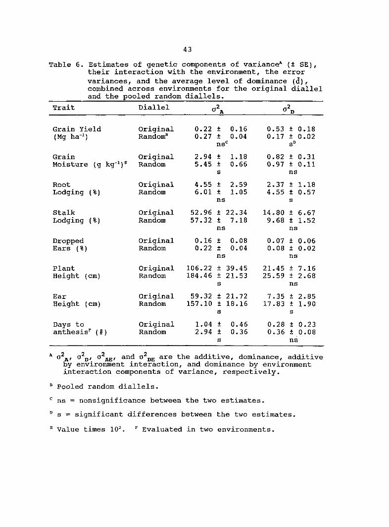
Estimates of additive (o^j^) and dominance (o^p) genetic
variance, their interaction with the environments and
o d̂e) ' their standard errors (SE) based on the combined
analysis across environments for eight traits are presented in
Table 6. Estimated variance components from the original
diallel always had higher standard errors than estimates from
the pooled random diallels. Estimates of from the pooled
random diallels were greater for all traits in comparison with
the original diallel. Four of the estimates from the
pooled random diallels were significantly different from the
original diallel estimates (Table 6). Similar estimates of o\
for grain yield, root lodging, stalk lodging and dropped ears
were obtained from the original diallel and the pool random
diallels. Estimates of for 3 traits (grain yield, root
lodging, ear height) were significantly different between the
pooled random diallels and the original diallel.
The estimate of for grain yield was 3.0 times greater
for the original diallel than for the pooled random diallels.
Therefore, most of the genetic variance for grain yield in the
original diallel was dominance. For the pooled random

26
diallels, the genetic variance for grain yield was composed
almost equally of additive and dominance. For both the
original diallel and the pooled random diallels, the majority
of the genetic variance for plant and ear height was additive.
Many estimates of and from the pooled random
diallels and the original diallel were of similar magnitudes.
Only three traits had estimates of and from the
pooled random diallels which were significantly different from
the original diallel. Estimates of for root and stalk
lodging were 1.7 and 2.0 times greater, respectively, for the
original diallel than for the pooled random diallels. In
contrast, estimates of for stalk lodging and days to
anthesis were almost 2.0 times greater for the pooled random
diallels relative to the original diallel.
Estimates of the average levels of dominance were greater
in the original diallel relative to the pooled random diallels
for all traits except root lodging and plant height. In both
the original diallel and the pooled random diallels for grain
yield and root lodging, estimates of the average levels of
dominance were in the overdominance range. For the other
traits, estimates of the average levels of dominance were in
the partial to complete dominance range. The average level of
dominance for grain yield was 2.0 times greater for the
original diallel than for the pooled random diallels.

27
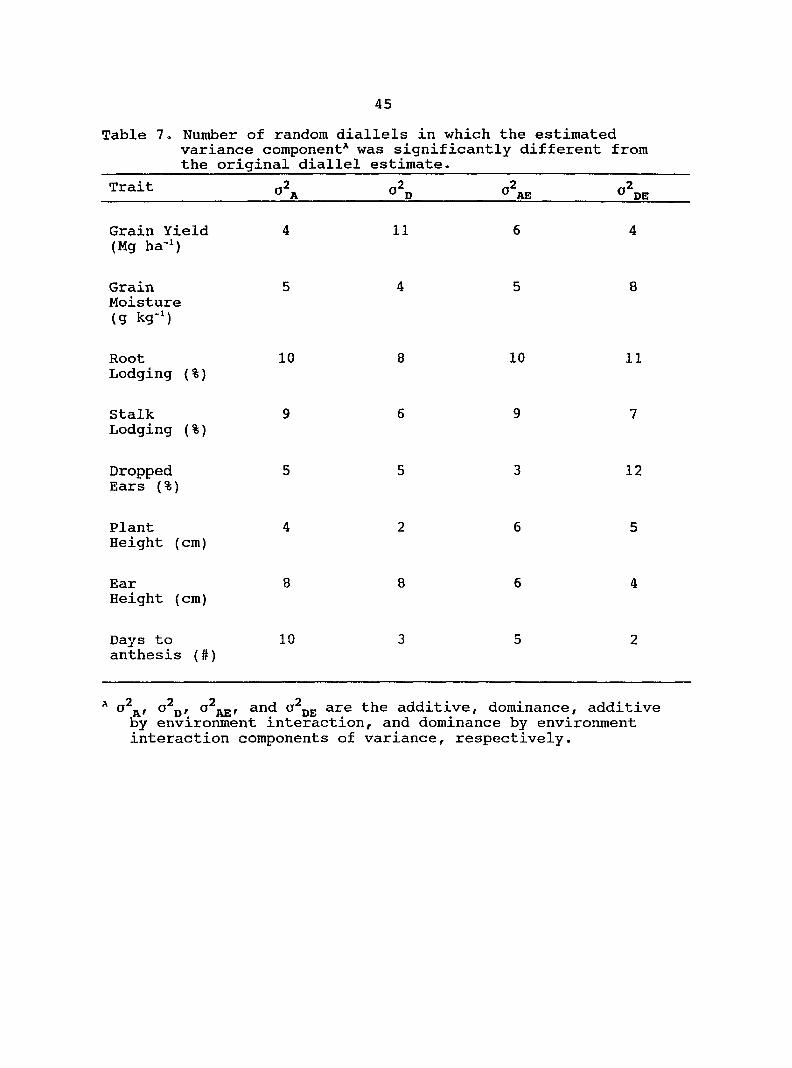
The number of random diallels for each trait that were
significantly different from the original diallel for the
estimated variance components are listed in Table 7,
For grain yield four of the 12 random diallels had
significantly different estimates of relative to the
original diallel. In contrast, 11 of the 12 random diallels
had significantly different estimates of for grain yield.
Root lodging and stalk lodging had the greatest number of
random diallels with significantly different estimates of
variance components compared with the original diallel. Plant
height had the least number of random diallels with
significantly different estimates of variance components.
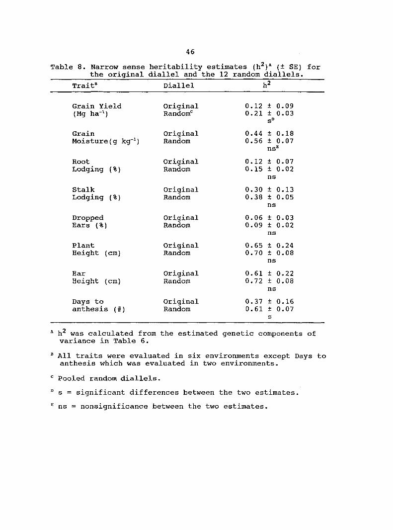
Narrow sense heritability (h ) estimates for the original
diallel and the pooled random diallels are presented in Table
8. For the original diallel, h^ estimates ranged from 0.06 for
dropped ears to 0.65 for plant height. Heritabilities
estimates for the pooled random diallels ranged from 0.09 for
dropped ears to 0.72 for ear height. In general, plant and ear
height had the highest h^ estimates while dropped ears and
root lodging had the lowest h^ estimates for both the original
and pooled random diallels.
Heritability estimates from the pooled random diallels
for each of the traits were always greater in comparison with
the original diallel h^ estimates. Only grain yield, and days
to anthesis had significantly different estimates of h^
28
between the original diallel and the pooled random diallels.
Discussion
Variance components were estimated with greater precision
from the pooled random diallels than from the original
diallel. Estimates of variance components from the pooled
random diallels were based on 96 inbred lines, or 364
crosses whereas estimates from the original diallel were based
on eight inbred lines, or 28 crosses. Components of
variance estimates from the original diallel, therefore,
always had greater standard errors. Hence the relative
magnitude of the standard errors for variance components from
the original diallel frequently determined if they were
significantly different from the estimates obtained from the
pooled random diallels.
Estimated variance components from the pooled random
diallels were considered to be representative of the true
genetic parameters of the Syn 5 population from which the
parents of the pooled random diallels were derived. The Syn 5
population was produced by random mating the bulk diallel
population five times. Therefore, it is believed that the Syn
5 population approaches or is in linkage equilibrium. Genetic
variances can be biased if they are not obtained from a large
random mating population in linkage equilibrium (Hallauer and
Miranda, 1988). Since the Syn 5 population represents a

29
relative large random mating population in linkage
equilibrium, the effects of linkage bias on the components of
variance estimates from the pooled random diallels are
probably minimal.
However, the same can not be stated for the estimated
variance components obtained from the original diallel.
Coupling phase linkages cause estimates of and to be
overestimated. Repulsion phase linkages cause estimates of
to be overestimated and estimates of to underestimated.
According to Hallauer and Miranda (1988) crossing highly
selected inbreds can result in the formation of repulsion
phase linkages. Inbreds from the opposite heterotic group more
than likely have different alleles influencing important
agronomic traits at the same loci. Hence crosses between Reid
Yellow Dent (RYD) inbreds (B73, B84, N28, B79) and Lancaster
Sure Crop (LSC) inbreds (B70, B77, Mol7, Va35) probably
resulted in predominantly repulsion phase linkages. Whereas,
crosses within the RYD and LSC heterotic group may have
frequently resulted in coupling phase linkages.
Given this linkage scenario, estimates of from the
original diallel may have been underestimated while estimates
of o^jj may have been overestimated from the original diallel.
The effects of linkage bias may account for some of the
differences in the relative magnitudes of the estimated

30
variance components from the original diallel. For example,
estimates of for all traits were underestimated in the
original diallel in comparison to the pooled random diallels.
However, the effect of linkage bias on a^jj in the original
diallel was not as evident for most traits. Only grain yield
and stalk lodging had greater estimates of for the
original diallel than for the pooled random diallels.
The effects of non-independent distribution of genes in
the parents of the diallel have been examined theoretical but
not empirically. Hayman (1954b) assessed the effects of the
failure of independent distribution of genes using the
graph and concluded that the average level of dominance may be
increased or may be decreased by non-independent distribution
of genes in the parents. Nassar (1965), based on a computer
simulation study, concluded that non-independent distribution
of genes in the parents usually resulted in the overestimation
of the average level of dominance. Our data, for some of the
traits, tend to support that the failure to achieve
independent distribution of genes in the parents results in
the average level of dominance being overestimated. For six
traits, the average level of dominance was slighter greater
from the original diallel than from the pooled random
diallels. The average level of dominance for grain yield was
almost 2.0 times greater for the original diallel than for the
pooled random diallels. It seems that five generations of
31
random mating reduced the effects of linkage bias for most of
the traits in the pooled random diallels. The indication of
overdominance in the original diallel for grain yield may be
explained by pseudooverdominance because of repulsion phase
linkages. Random mating for several generations has been used
to determine whether repulsion phase linkage bias is
responsible for pseudooverdominance effects in maize (Gardner
and Lonnquist, 1959; Han and Hallauer, 1989). Lonnquist (1980)
presented unpublished data from Gardner and Lonnquist (1961)
which showed that the average level of dominance for grain
yield decreased from 1.75 to 0.62 with 16 generations of
random mating. Linkage effects, mainly repulsion in the
original diallel, may also have influenced estimates of
and because the average level of dominance estimates for
six traits was reduced in the pooled random diallels.
Heritability estimates from both the original diallel and
the pooled random diallels generally agree with previous
estimates of h^ in maize populations (Hallauer and Miranda,
1988). That is complex traits, such as yield, had lower h^
estimates and less complex traits, such has plant and ear
height, had greater h^ estimates. The relative magnitudes of
the h^ estimates for most of the traits except days to
anthesis were similar for the original diallel and the pooled
random diallels. Greater standard errors for h^ estimates from
the original diallel can be attributed to the precision of

32
estimating and o^p.
Estimates of genetic parameters for a population can be
very useful to plant breeders in deciding the appropriate
breeding strategy that will utilize the genetic variance
present. Estimates of variance components can be used to
calculate heritabilities, genetic correlations, and predicted
gains from selection.
Even though estimates of and for some traits were
similar for the original diallel and for the pooled random
diallels, they are useless since a reference population does
not exist. A descendant reference population could be created
by random mating the parents of the diallel for several
generations (Kuehl et al. 1968; Wright, 1985). Since the fixed
parents of a diallel do not represent a population in
equilibrium, Kuehl et al. (1968) and Wright (1985) consider
this the only meaningful reference population for the
estimates of genetic variance components. For hybrids crops,
such as maize, the combining of two heterotic groups to create
a descendant reference population to estimate genetic
parameters is neither logical or meaningful.
Although this experiment may not have provided conclusive
evidence on the effects of non-independent distribution of
genes in the parents on estimating genetic parcuneters, one can
not argue with the reference population issue. Therefore, the
diallel mating design should only be used to estimate genetic

33
variance components when the parents of the diallel have been
randomly selected from a population in linkage equilibrium.
References
Baker, R.J, 1978. Issues in diallel analysis. Crop Sci. 18:533-536.
Cockerham, C.C. 1956. Analysis of quantitative gene action. Brookhaven Symp. Biol. 9:53-68.
Comstock, R.E., and H.F. Robinson. 1948. The components of genetic variance in populations of biparental progenies and their use in estimating the average degree of dominance. Biometrics 4:254-266.
Dickerson, G.E. 1969, Techniques for research in quantitative animal genetics. In Techniques and Procedures in Animal Science Research. Am. Soc. Anim. Sci. p.36-79.
Gardner, C.O., and J.H. Lonnquist. 1959. Linkage and the degree of dominance of genes controlling quantitative characters in maize. Agron. J. 51:524-28.
Gilbert, N.E.G. 1958. Diallel cross in plant breeding. Heredity 12:477-492.
Griffing, B. 1956b. Concepts of general and specific combining ability in relation to diallel crossing systems. Aust. J. Biol. Sci. 9:463-493.
Hallauer, A.R., S.A. Eberhart, and W.A. Russell. 1974. Registration of maize germplasm. Crop Sci. 14:341-342.
Hallauer, A.R., and J.B. Miranda, Fo. 1988. Quantitative genetics in maize breeding. 2nd ed. Iowa State Univ. Press, Ames, lA.
Han, G.C., and A.R. Hallauer. 1989. Estimates of genetic variability in F2 maize populations. J. Iowa Acad. Sci. 96(1):14-19.
Hayman, B.I. 1954b. The theory and analysis of diallel crosses. Genetics 39;789-809.
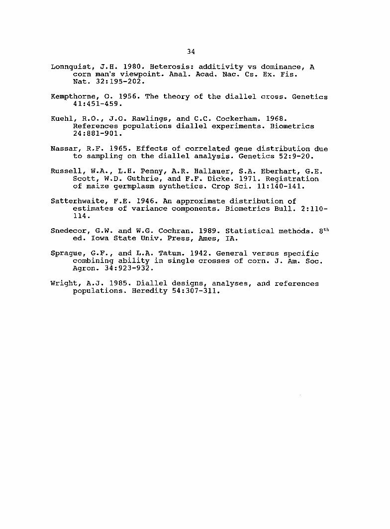
34
Lonnquist, J.H. 1980. Heterosis; additivity vs dominance, A corn man's viewpoint. Anal. Acad. Nac. Cs. Ex. Fis. Nat. 32:195-202.
Kempthorne, O. 1956. The theory of the diallel cross. Genetics 41:451-459.
Kuehl, R.O., J.O. Rawlings, and C.C. Cockerham. 1968. References populations diallel experiments. Biometrics 24:881-901.
Nassar, R.F. 1965. Effects of correlated gene distribution due to sampling on the diallel analysis. Genetics 52:9-20.
Russell, W.A., L.H. Penny, A.R. Hallauer, S.A. Eberhart, G.E, Scott, W.D. Guthrie, and F.F. Dicke. 1971. Registration of maize germplasm synthetics. Crop Sci. 11:140-141.
Satterhwaite, F.E. 1946. An approximate distribution of estimates of variance components. Biometrics Bull. 2:110-114.
Snedecor, G.W. and W.G. Cochran. 1989. Statistical methods. ed. Iowa State Univ. Press, Ames, lA.
Sprague, G.F., and L.A. Tatum. 1942. General versus specific combining ability in single crosses of corn. J. Am. Soc. Agron. 34:923-932.
Wright, A.J. 1985. Diallel designs, analyses, and references populations. Heredity 54:307-311.

35
ORIGINAL DIALLEL CROSS (B70, B73, B77, 879, B84, Mo17, N28, Va35)
1 20 seeds/F1 to form Bulk Diallel
1 Intermated Bulk Diallel to form
Syn 1 - 500 seed bulk
i Intermated Syn 1 until the Syn 5
i Syn 5 ® all plants to produce
100 unselected S^ lines
I SiS were advanced to the Sg by
single-seed descent
i 100 Sg lines were (8)
Each Sg row was bulk harvested to obtain S7 bulk lines
i Twelve 8 parent diallels were made using 96 of 100
unselected derived lines from the bulk diallel
Figure 1. Outline of the breeding scheme used to produce 100 unselected lines that were used to generate the 12 random diallels.

Table 1. Analysis of variance showing the sources of variation, degrees of freedom (df), expected mean squares (EMS), and F-test for the combined analysis across environments for each diallel.
Source df MS E(MS) F-test
Env. (E) 0-1 MS 5 0^ + + rcO% F^
Replication/E e(r-l) MS 4 0=^ + HS4/MS1
Crosses n<n-l) /2-l'^ MS 3 0^ + rea% MS3/MS2
GCA n-1 MS31 + + + ^( '^-2)C%(gci i ) + re(n-2)a '^ F"
SCA n(n-3)/2 MS32 + B(SC&)
MS32/MS22
Crosses x E (c-1)(e-1) MS 2 0® + rO^ CB
MS2/MS1
GCA X E (n-1)(e-1) MS21 0^ + E(SCA)
+ r (n-2)0%j^, MS21/MS22
SCA X E {n(n-3)/2}(e-l) MS22 a' + B(EG&)
MS22/MS1
Error e(r-l)(C-1) MSl o'
F* (MS5 + MSl)/(MS4 + MS2)
F® (MS31 + MS22)/(MS32 + MS21)
n(n-l)/2-l = c-1

Table 2. Analysis of variance showing the sources of variation, degrees of freedom (df), and expected mean squares (EMS) for traits pooled over sets for one environment.
Source df MS E(MS) F-test
Sets (S) s-1 MS 4 + + rca\ (MS4 +MS1)/(MS3 + MS2)
Reps/S s(r-l) MS3 + MS3/MSI
Crosses/s n(n-l)/2-l* (s-1)
MS2 + MS2/MS1
GCA/s (n-1)(s-1) MS21 0^ + ^("-2)0^gca/S MS21/MS22
SCA/S {n(n-3)/2}(3-l) MS22 + SCiV/S MS22/MS1
Error e(r-l)(c-1) MSI 0=^
^i(n-l)/2-l = c-1
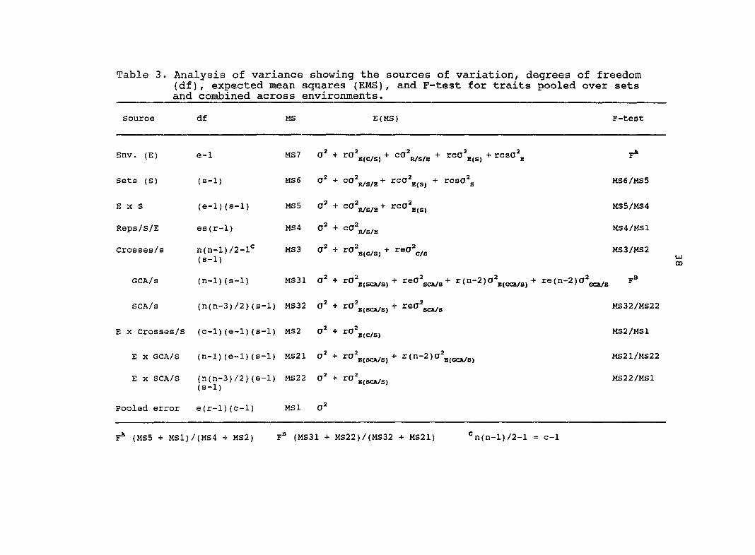
Table 3. Analysis of variance showing the sources of variation, degrees of freedom (df), expected mean squares (EMS), and F-test for traits pooled over sets and combined across environments.
Source df MS E(MS) F-test
Env. (E) e-1 MS 7 0^ + B(C/S) * •^O'R/S/E + + ̂ =30%
Sets (S) (3-1) MS 6 0== + MS6/MS5
E X S (e-1)(3-1) MS5 + MS5/MS4
Reps/S/E es(r-1) MS4 0^ + K/S/B MS4/MS1
Crosses/s n(n-l)/2-l'^ (3-1)
MS3 + MS3/MS2
GCA/s (n-l)(3-1) MS31 + rO^ B(SC2V/S)
re(n-2)02^3 F=
SCA/3 {n(n-3)/2}(3 -1) MS32 + rO^ " s(scAys) MS32/MS22
E X Crosses/s (c-1)(e-1)(3 -1) MS2 + B(C/S)
MS2/HS1
E X GCA/S (n-l)(e-1)(s -1) MS21 0=® + 2 K(SC&/S)
+ r(n-2)0 MS21/MS22
E X SCA/S {n(n-3)/2}(e (3-1)
-1) MS22 + ro^ ^ B(SCA/S)
MS22/MS1
Pooled error e(r-l)(C-1) MSI 0^
(MS5 + MS1)/(MS4 + MS2) F® (MS31 + MS22)/(MS32 + MS21) '^n(n-l)/2-l = c-1

Table 4. Mean squares of the analysis of variance combined across six environments in 1993 & 1994 for the original diallel.
Source of Variation
df Grain Yield
Grain Moisture
Root Lodging
Stalk Lodging
Dropped Ears
(mg ha"^) (g (%)
Env.(E) 5 186.41** 583.51** 407.14** 358.93** 9.60**
Reps/E 6 2.03** 9.22** 15.93 226.19** 1.35
Crosses 27 9.61** 41.33** 103.40** 801.64** 3.86**
GCA 7 16.38 124.52** 267.30* 2341.96** 8.33*
SCA 20 7.24** 12.21** 46.03** 262.52** 2.30
E X Crosses 135 1.27** 4.04** 32.47** 129.78** 1.52
E X GCA 35 2.25** 8.74** 75.07** 257.97** 1.58
E X SCA 100 0.93* 2.39** 17.56** 84.92 1.50
Error 160 0.65 1.34 8.92 73.61 2.41
Mean C.V.%
6.48 12.45
25.11 4.61
2.12 140.85
18.31 46.86
0.67 231.92
^ Value times 10^.
*, ** significant at the 0.05 and 0.01 probability levels, respectively.

Table 4. (Continued)
Source of Variation
df Plant Height
Ear Height
df Days to Anthesis®
-(cm) (no.)
Env.(E) 5 5984.86** 3636.65** 1 195.57**
Reps/E 6 256.27** 90.43** 2 18.04**
Crosses 27 1292.83** 679.14** 27 6.09**
GCA 7 4173.94** 2296.82** 7 15.83*
SCA 20 284.45** 112.95** 20 2.68
E X Crosses 135 43.93** 37.27** 27 1.72
E X GCA 35 92.35** 73.15** 7 2.21
E X SCA 100 26.99 24.72** 20 1.55
Error 160 23.64 19.86 52 1.27
Mean C.V.%
245.10 1.98
129.90 3.43
88.18 1.28
®Days to anthesis was evaluated at 2 environments.
«,** Significant at the 0.05 and 0.01 probability levels, respectively.

Table 5. Mean squares of the analysis of variance pooled over 12 random diallels and combined across six environments in 1993 & 1994.
Source of Variation
df Grain Yield
Grain Moisture
Root Lodging
Stalk Lodging
Dropped Ecirs
(mg ha"^) (g kg-^)^ (%)
Env.(E) 5 2335.34** 4733.45** 1312.94** 5406.31** 84.95**
Sets (S) 11 83.82** 596.24** 701.20** 7157.79** 22.79**
E X s 55 4.36* 63.02** 138.08** 685.20** 4.57**
Reps/S/E 72 2.71** 10.08 20.22** 155.48** 2.52
crosses/s 324 5.82" 66 .60** 143.43** 755.63** 5.30**
GCA/S 84 14.23** 216.29** 338.44** 2349.63** 11.53**
SCA/S 240 2.88** 14.21** 75.17** 197.73** 3.12**
E X crosses/s 1620 1.12** 4.09** 32.66** 102.33** 2.25**
E X GCA/S 420 2.25** 8.44** 67.32** 167.76** 2.67**
E X SCA/S 1200 0.73** 2.57** 20.54** 79.43** 2.10**
Pooled error 1926 0.51 1.90 15.73 57.53 2.01
Mean c.v.%
5.98 11.94
24.28 5.65
1.62 244.81
15.69 48.33
0.63 224.68
^ value times 10^.
*,** significant at the 0.05 and 0.01 probability levels, respectively.

Table 5. (Continued)
Source of Variation
df Plant Height
Ear Height
df Days to Anthesis®
(cm)- (no.)
Env.(E) 5 6823.55** 35549.14** 1 6545.50**
Sets (S) 11 28738.70** 15736.04** 11 187.44*
E X S 55 912.83* 1027.51** 11 60.65**
Repa/s/E 72 294.21** 231.25** 24 9.91**
Crosses/S 324 2089.57** 1728.12** 324 12.40**
GCA/S 84 7051.96** 5950.41** 84 39.19**
SCA/S 240 352.74** 250.32** 240 3.02**
E X Crosses/S 1620 60.91** 47.88** 324 1.81**
E X GCA/S 420 104.43** 80 .67** 84 2.42**
E X SCA/S 1200 45.68* 36.40** 240 1.60**
Pooled error 1942 40.95 32 .35 590 1.08
Mean C.V.%
227.89 2.81
116.78 4.87
86.43 1.20
® Days to anthesis was evlauated at 2 environments.
*,** significant at the 0.05 and 0.01 probability levels, respectively.
43
Table 6. Estimates of genetic components of variance* (± SE), their interaction with the environment, the error variances, and the average level of dominance (d), combined across environments for the original diallel and the pooled random diallels.
Trait Diallel (j2 A O
Grain Yield (Mg ha"^)
Original Random®
Grain Original Moisture (g kg"^)® Random
Root Lodging (%)
Stalk Lodging (%)
Dropped Ears (%)
Plant Height (cm)
Ear Height (cm)
Days to anthesis^ (#)
Original Random
Original Random
Original Random
Original Random
Original Random
Original Random
0.22 + 0.15 0.27 ± 0.04
ns*^
2.94 ± 1.18 5.45 ± 0.66
s
4.55 ± 2.59 6.01 ± 1.05
ns
52.96 ± 22.34 57.32 ± 7.18
ns
0 . 1 6 ± 0 . 0 8 0.22 ± 0.04
ns
106.22 ± 39.45 184.46 ± 21.53
59.32 ± 21.72 157.10 ± 18.16
s
1.04 ± 0.46 2.94 ± 0.36
s
0.53 ± 0.18 0.17 ± 0.02
s°
0.82 ± 0.31 0.97 ± 0.11
nS
2.37 ± 1.18 4.55 ± 0.57
s
14.80 ± 6.67 9.68 ± 1.52
ns
0.07 ± 0.06 0 . 0 8 ± 0 . 0 2
ns
21.45 ± 7.16 25.59 ± 2.68
ns
7.35 ± 2.85 17.83 ± 1.90
0.28 ± 0.23 0.36 ± 0.08
ns
and are the additive, dominance, additive by environment interaction, and dominance by environment interaction components of variance, respectively.
° Pooled random diallels.
^ ns = nonsignificance between the two estimates.
° s = significant differences between the two estimates.
® Value times 10^. ^ Evaluated in two environments.

Table 6. (Continued)
44
AE OE
0 . 2 2 ± 0 . 0 6 0.25 ± 0.02
ns
1.06 ± 0.24 0.98 ± 0.07
ns
17.36 ± 3.32 10.32 ± 0.63
s
28.84 ± 7.07 14.72 ± 1.41
0.01 + 0.05 0.09 ± 0.02
10.89 ± 2.53 9.79 ± 0.88
ns
8.07 ± 2-01 7.38 ± 0.68
ns
0.11 ± 0.13 0.14 + 0.05
ns
0.14 ± 0.08 0 . 1 1 ± 0 . 0 2
ns
0.53 ± 0.18 0.33 ± 0.06
5.37 ± 1.19 4.01 ± 0.34
s
5.65 ± 5.96 10.95 ± 1.87
ns
-.46 0.13 0.04 ± 0.05
s
1.67 ± 1.91 2,36 ± 1.14
ns
2.34 ± 1.75 2.03 ± 0.90
ns
0.14 ± 0.26 0.26 ± 0.08
ns
0.65 ± 0.07 0.51 ± 0.02
1.34 ± 0.15 1.90 ± 0.06
8.92 ± 0.99 15.73 ± 0.51
73.61 ± 8.18 57.53 ± 1.85
2.41 ± 0.27 2 . 0 1 ± 0 . 0 6
23.64 ± 2.63 40.95 ± 1.31
19.86 ± 2.21 32.35 ± 1.04
1.27 ± 0.24 1.08 ± 0.06
2.19 1 . 1 2
0.75 0 . 6 0
1 . 0 2 1.23
0.75 0.58
0.93 0.85
0.40 0.53
0.25 0.23
0.73 0.49
45
Table 7. Number of random diallels in which the estimated variance component* was significantly different from the original diallel estimate.
Trait (3^ " A " D " AE " DE
Grain Yield 4 11 6 4 (Mg ha~^)
Grain 5 4 5 8 Moisture (g kg-i)
Root 10 8 10 11 Lodging (%)
Stalk 9 6 9 7 Lodging (%)
Dropped 5 5 3 12 Ears (%)
Plant 4 2 6 5 Height (cm)
Ear 8 8 6 4 Height (cm)
Days to 10 3 5 2 anthesis {#)
* o^j^r o^jj, ®^AE' additive, dominance, additive by environment interaction, and dominance by environment interaction components of variance, respectively.
46
Table 8. Narrow sense heritability estimates (h^)* (± SE) for the original diallel and the 12 random diallels.
Trait® Diallel
Grain Yield (Mg ha'^)
Original Random*^
0.12 ± 0.09 0.21 ± 0.03
Grain Moisture (g kg"^)
Root Lodging (%)
Stalk Lodging (%)
Dropped Ears (%)
Plant Height (cm)
Ear Height (cm)
Days to anthesis (#)
Original Random
Original Random
Original Random
Original Random
Original Random
Original Random
Original Random
0.44 ± 0.18 0.56 ± 0.07
ns®
0.12 ± 0.07 0.15 ± 0.02
ns
0.30 ± 0.13 0.38 ± 0.05
ns
0.06 ± 0.03 0.09 ± 0.02
ns
0.65 ± 0.24 0.70 ± 0.08
ns
0 . 6 1 ± 0 . 2 2 0.72 ± 0.08
ns
0.37 ± 0.16 0.61 ± 0.07
s
h^ was calculated from the estimated genetic components of variance in Table 6,
® All traits were evaluated in six environments except Days to anthesis which was evaluated in two environments.
Pooled random diallels.
° s = significant differences between the two estimates.
® ns = nonsignificance between the two estimates.
47
GENERAL CONCLUSION
The objective of this study was to test the assumption
that to obtain accurate and valid estimates of genetic
variance components using the diallel mating design the genes
in the parents must be independently distributed. Only parents
that have been randomly selected from a population in linkage
equilibrium satisfy this assumption.
The results from this study indicate that non-independent
distribution of genes in the parents can cause estimates of
additive and dominance variances to be either overestimated or
underestimated. The effect of linkage bias on additive
variance estimates for all traits was evident while only a few
estimates of dominance variances seem to be affected by
linkages in the original diallel. In addition, the average
level of dominance for most traits was overestimated with non-
independent distribution of genes.
The diallel mating design can provide valuable
information if properly analyzed and interpreted. If the
parents of a diallel are selected based on performance, then a
fixed effects model (Model I) should be used in the analysis.
Only estimates of general and specific combining ability
effects are valid with Model I. If the parents of a diallel
represent a random sample from a population in linkage
equilibrium then a random effects model (Model II) should be
used in the analysis. With Model II estimates of additive and
48
dominance variances can be obtained and inferences about the
population from which the parents were selected can be made.

49
LITERATURE CITED
Baker, R.J. 1978. Issues in diallel analysis. Crop Sci. 18:533-536.
Bhullar, G.S., K.S. Gill, and A.S. Khehra. 1979. Combining ability analysis over F^-F^ generations in diallel crosses of bread wheat. Theor. Appl. Genet. 55:77-80.
Christie, B.R., and V.I. Shattuck. 1992. p. 9-36. The diallel cross; design, analysis and use for plant breeders. In J. Janick (ed.) Plant Breeding Reviews. John Wiley & Sons, Inc.
Cockerham, C.C. 1956. Analysis of quantitative gene action. Brookhaven Symp. Biol. 9:53-68.
Eberhart, S.A., and C.O. Gardner. 1966. A general model for genetic effects. Biometrics 22:864-881.
Gardner, C.O., and S.A. Eberhart. 1966. Analysis and interpretation of the variety cross diallel and related populations. Biometrics 22:439-452.
Gilbert, N.E.G. 1958. Diallel cross in plant breeding. Heredity 12:477-492.
Griffing, B. 1956a. A generalized treatment of diallel crosses in quantitative inheritance. Heredity 10:31-50.
Griffing, B. 1956b. Concepts of general and specific combining ability in relation to diallel crossing systems. Aust. J. Biol. Sci. 9:463-493.
Hallauer, A.R., and J.B. Miranda, Fo. 1988. Quantitative genetics in maize breeding. 2""^ ed. Iowa State Univ. Press, Ames, lA.
Hayman, B.I. 1954a. The analysis of variance of diallel tables. Biometrics 10:235-244.
Hayman, B.I. 1954b. The theory and analysis of diallel crosses. Genetics 39:789-809.
Hayman, B.I. 1958. The theory and analysis of diallel crosses. II Genetics 43:63-85.
Hayman, B.I. 1960. The theory and analysis of diallel crosses. III Genetics 45:155-172.

50
Hayman, B.I. 1963. Notes on diallel cross theory, p. 571-578, In Statistical genetics and plant breeding. NAS-NRC #982.
Hayward, M.D. 1979. The application of the diallel cross to outbreeding crop species. Euphytica 28:729-737.
Jinks, J.L., and B.I. Hayman. 1953. The analysis of diallel crosses. Maize Genetics Coop. Newsletter 27:48-54.
Kempthorne, O. 1956. The theory of the diallel cross. Genetics 41:451-459.
Kempthorne, O., and R.N. Curnow. 1961. The partial diallel cross. Biometrics 17:229-250.
Kuehl, R.O., J.O. Rawlings, and C.C. Cockerham. 1968. References populations diallel experiments. Biometrics 24:881-901.
Lush, J.L. 1945. Animal breeding plans, 3""^ ed. Iowa State Univ. Press, Ames, lA.
Matzinger, D.F., and O. Kempthorne. 1956. The modified diallel table with partial inbreeding and interactions with environment. Genetics 41:822-833.
Nassar, R.F. 1965. Effects of correlated gene distribution due to sampling on the diallel analysis. Genetics 52:9-20.
Pederson, D.G. 1971. The estimation of heritability and degree of dominance from a diallel cross. Heredity 27:247-264.
Sokol, M.J., and R.J. Baker. 1977. Evaluation of the assumptions required for the genetic interpretation of diallel experiments in self-pollinating crops. Can. J. Plant Sci. 57:1185-1191.
Sprague, G.F., and L.A. Tatum. 1942. General versus specific combining ability in single crosses of corn. J, Am. Soc. Agron. 34:923-932.
Wright, A.J. 1985, Diallel designs, analyses, and references populations. Heredity 54:307-311,

51
APPENDIX
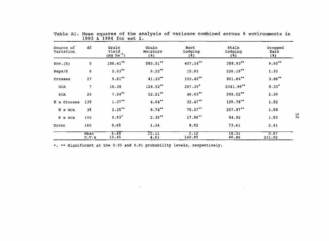
Table Al. Mean squares of the analysis of variance combined across 6 environments in 1993 & 1994 for set 1.
source of Variation
df Grain Yield
(mg ha"^)
Grain Moisture (%)
Root Lodging (%)
Stalk Lodging (%)
Dropped Ears (%)
Env.(E) 5 186.41" 583.51** 407.14** 358.93** 9.60**
Reps/E 6 2.03** 9 .22 15.93 226.19** 1.35
Crosses 27 9.61** 41.33** 103.40** 801.64** 3.86**
GCA 7 16 .38 124.52** 267 .30* 2341.96** 8.33*
SCA 20 7.24** 12.21** 46.03** 262.52** 2.30
E X Crosses 135 1.27** 4.04** 32.47** 129.78** 1.52
E X GCA 35 2.25** 8.74** 75.07** 257.97** 1.58
E X SCA 100 0,93* 2.39** 17.56** 84.92 1.50
Error 160 0.65 1.34 8.92 73.61 2.41
Mean c,v.%
6.48 12.45
25.11 4.61
2.12 140.85
18.31 46.86
0.67 231.92
*, ** significant at the 0.05 and 0.01 probability levels, respectively.

Table Al. (Continued)
Source of variation
df Plant Height (cm)
Ear Height (cm)
df Days to Anthesis* (no.)
Env.(E) 5 5984.86" 3636.65** 1 195.57**
Reps/E 6 256.27" 90.43** 2 18.04**
crosses 27 1292.83** 679.14** 27 6.09**
GCA 7 4173.94** 2296.82** 7 15.83*
SCA 20 284.45** 112.95** 20 2.68
E X Crosses 135 43.93** 37.27" 27 1.72
E X GCA 35 92.35** 73.15** 7 2.21
E X SCA 100 26.99 24.72** 20 1.55
Error 160 23.64 19.86 52 1.27
Mean C.V.%
245.10 1.98
129.90 3.43
88.18 1.28
* Days to anthesis was evaluated at 2 environments.
*,** significant at the 0.05 and 0.01 probability levels, repsectively.

Table A2. Mean squares of the analysis of variance combined across 6 environments in 1993 & 1994 for set 2.
Source of Variation
df Grain Yield
(mg ha"^)
Grain Moisture (%)
Root Lodging (%)
Stalk Lodging (%)
Dropped Ears (%)
Env.(E) 5 153.70" 569.36** 83.54** 1631.70** 13.37**
Reps/E 6 3.68** 7.81** 1.68 264.23** 2.13
Crosses 27 2.50** 52.32** 40.64** 443.18** 8.95**
GCA 7 2.55 170.02** 75.78 1186.91** 18.20*
SCA 20 2.49** 11.12** 28.34** 182.87** 5.71*
E X Crosses 135 1.17** 4.45** 11.50** 104.48** 3.46**
E X GCA 35 3.10** 11.72** 17.87** 228.01** 4.23
E X SCA 100 0.50 1.91* 9.27** 61.24 3.20*
Error 162 0.46 1.34 5.47 54.74 2.25
Mean C.V.%
6.01 11.23
23.97 4.83
1.01 231.52
15.66 47.23
0.81 185.17
*, ** significant at the 0.05 and 0.01 probability levels, respectively.
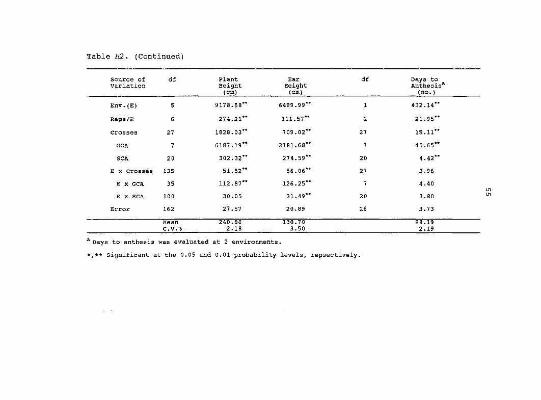
Table A2. (Continued)
source of Variation
df Plant Height (cm)
Ear Height (cm)
df Days to Anthesis* (no.)
Env.(E) 5 9178.58** 6489.99** 1 432.14**
Reps/E 6 274.21** 111.57** 2 21.95**
Crosses 27 1828.03** 709 .02** 27 15.11**
GCA 7 6187.19** 2181.68** 7 45.65**
SCA 20 302.32** 274.59** 20 4.42**
E X Crosses 135 51.52** 56.06** 27 3.96
E X GCA 35 112.87** 126.25** 7 4.40
E X SCA 100 30.05 31.49** 20 3.80
Error 162 27.57 20.89 26 3.73
Mean c.v.%
240.80 2.18
130.70 3.50
88.19 2.19
^ Days to anthesis was evaluated at 2 environments.
*,** Significant at the 0.05 and 0.01 probability levels, repsectively.

Table A3. Mean squares of the analysis of variance combined across 6 environments in 1993 & 1994 for set 3.
Source of Variation
df Grain Yield
(mg ha"^)
Grain Moisture (%)
Root Lodging (%)
Stalk Lodging (%)
Dropped Ears (%)
Env.(E) 5 168.97" 473.68** 183.88** 1398.72** 24.86**
Reps/E 6 3.69** 6.37** 25.34" 149.90** 2.34
Crosses 27 5.57" 72.90** 10.08 1157.94** 15.34"
GCA 7 14.98** 254.40** 26.99 3479.49** 32.77*
SCA 20 2.27" 9.37** 4.16 345.40** 9.24*
E X croases 135 0.83** 3.98** 9.22* 105.44** 4.46**
E X GCA 35 1.75" 10.27** 22.43** 204.51** 4.73
E X SCA 100 0.51 1,77 4.60 70.77 4.37**
Error 162 0.56 1.48 6.72 67.74 2.63
Mean C.V.%
6.32 11.88
23.44 5.19
0.90 287.95
17.75 46 .38
0.98 165.42
*, ** significant at the 0.05 and 0.01 probability levels, respectively.

Table A3. (Continued)
Source of df Plant Ear df Days to Variation Height Height Anthesis*
(cm) (cm) (no.)
Env.(E) 5 8285.70" 8435.91" 1 270.32**
Reps/E 6 319.28" 202.02" 2 6.52**
Crosses 27 3116.89" 2240.94" 27 5.59*
GCA 7 11057.73" 8375.90** 7 16.79
SCA 20 337.60" 93.71** 20 1.67
E X Crosses 135 49.93" 40.46** 27 2.32**
E X GCA 35 76 .70" 79.08** 7 5.18**
E X SCA 100 40.57 26.95 20 1.32*
Error 162 36.65 25.40 54 0.63
Mean c.v.%
223.41 2.71
112.21 4.49
84.21 0.94
^Days to anthesis was evaluated at 2 environments.
*,** significant at the 0.05 and 0.01 probability levels, repsectively.

Table A4. Mean squares of the analysis of variance combined across 6 environments in 1993 & 1994 for set 4.
Source of Variation
df Grain Yield
(mg ha"^)
Grain Moisture (%)
Root Lodging (%)
Stalk Lodging (%)
Dropped Ears (%)
Env.(E) 5 178.53" 511.60** 923.22** 413.71** 2.48**
Reps/E 6 3.81" 5.57" 25.03 348.79** 0.56
Crosses 27 4.99" 87 .07** 470.91** 1446.23** 1.07
GCA 7 12.92** 283.61** 1268.22** 4598.68** 2.33
SCA 20 2.21** 18.28** 191.85** 342.87** 0,63
E X Crosses 135 1.36** 3.44" 126.07** 179.98** 0.99
E X GCA 35 2.86** 8.53** 285.95** 281.92** 1.16
E X SCA 100 0.83* 1.66 70.12** 144.30** 0.93
Error 161 0.55 1.54 43.64 85.18 0.79
Mean C.V.%
5.67 13.12
22.99 5.40
4.11 160.74
21.68 42.57
0.31 287.05
*, ** significant at the 0.05 and 0.01 probability levels, respectively.

Table A4. (Continued)
Source of Variation
df Plant Height (cm)
Ear Height (cm)
df Days to Anthesis* (no.)
Env.(E) 5 6971.54" 6131.30" 1 292.51**
Reps/E 6 396.94" 233.19" 2 8.26**
Crosses 27 1766.85" 3163.09" 27 7 .10**
GCA 7 6191.87" 11648.33** 7 24.91**
SCA 20 218.10" 193.25** 20 0.87
E X Crosses 135 53.69" 60.34 27 1.21
E X GCA 35 105.23" 94.63** 7 0.87
E X SCA 100 35.66 48.34 20 1.33
Error 161 30.76 47.85 53 0.89
Mean c.v. %
223.13 2.49
119.90 5.57
86.24 1.09
^ Days to anthesis was evaluated at 2 environments.
«,** significant at the 0.05 and 0.01 probability levels, repsectively.

Table A5. Mean squares of the analysis of variance combined across 6 environments in 1993 & 1994 for set 5.
source of Variation
df Grain Yield
(mg ha"^)
Grain Moisture (%)
Root Lodging (%)
Stalk Lodging (%)
Dropped Ears <%)
Env.(E) 5 205.13" 287.97" 5.22" 165.89** 1.86**
Reps/E 6 3.12" 12.59" 2.20 167.70** 0.75
Crosses 27 3.25" 55.63" 4.75** 315.21** 1.87"
GCA 7 5.96 178.77** 6.63** 943.54** 3.14
SCA 20 2.30" 12.53" 4.09** 95.29** 1.43*
E X Crosses 135 0.85" 4.84** 1.69" 45.19 0.74
E X GCA 35 1.72" 7.28* 1.43 70.29** 0.77
E X SCA 100 0.54 3.98** 1.77* 36.41 0.73
Error 162 0.47 2.51 1.22 32.47 0.85
Mean c.v.%
6.20 11.04
23.75 6.67
0.28 393.75
10.17 56.05
0.28 329.79
*, ** significant at the 0.05 and 0.01 probability levels, respectively.

Table A5. (Continued)
Source of Variation
df Plant Height (cm)
Ear Height (cm)
df Days to Anthesis* (no.)
Env.(E) 5 5932.62" 4854.52** 1 122.22**
Reps/E 6 443.08" 423.21** 2 12.01"
Crosses 27 4808.89** 3352.82** 27 11.44**
GCA 7 17523.74** 12250.72** 7 37.07**
SCA 20 358.70** 236.76** 20 2.47*
E X Crosses 135 52.89* 49.13** 27 1.13*
E X GCA 35 61.82 59.46 7 1.12
E X SCA 100 49.77* 45.52" 20 1.14*
Error 162 36.17 28.08 54 0.64
Mean C.V.%
216.03 2.78
107.83 4.92
87.31 0.92
* Days to anthesis was evaluated at 2 environments.
*,** significant at the 0.05 and 0.01 probability levels, repsectively.

Table A6. Mean squares of the analysis of variance combined across 6 environments in 1993 & 1994 for set 6.
Source of Variation
df Grain Yield
(mg ha~^)
Grain Moisture (%)
Root Lodging (%)
Stalk Lodging (%)
Dropped Ears (%)
Env.(E) 5 182.88" 392.77" 6.66** 1169.91** 16.10**
Reps/E 6 3.50" 15.94" 1.25 177.41** 8.38**
Crosses 27 4.90" 69 .27" 1.16 1680.80** 5.36*
GCA 7 6.36 199.05** 1.00 5449.66** 15.85**
SCA 20 6.84" 23.85** 1.22 361.70** 1.68
E X Crosses 135 0.45 3.66** 1.38* 125.01 3.30
E X GCA 35 2.18" 6.74" 1.12 157.66 4.01
E X SCA 100 0.77 2.58* 1.47* 113.57* 3.06
Error 162 0.65 1.78 1.05 81.37 2.64
Mean C.V.%
5.90 13.67
23.43 5.70
0.20 512.63
20.63 43.72
0.88 184.46
*, ** significant at the 0.05 and 0.01 probability levels, respectively.

Table A6. (Continued)
Source of Variation
df Plant Height (cm)
Ear Height (cm)
df Days to Anthesis* (no.)
Env.(E) 5 3697.78" 3927.63** 1 255.01**
Rssps/E 6 275.48" 324.01** 2 9.58"
Crosses 27 1937.59" 1321.37** 27 13.69**
GCA 7 5715.00" 4221.08** 7 42.39**
SCA 20 615.50" 306.48** 20 3.64*
E X Crosses 135 50.43** 36.64** 27 1.66**
E X GCA 35 83.61** 62.66** 7 2.51
E X SCA 100 38.81** 27.53** 20 1.36*
Error 162 29.58 22.72 54 0.54
Mean C.V.%
224.23 2.43
115.91 4.11
85.54 0.86
* Days to anthesis was evaluated at 2 environments.
*,** significant at the 0.05 and 0.01 probability levels, repsectively.

Table A7. Mean squares of the analysis of variance combined across 6 environments in 1993 & 1994 for set 7.
source of Variation
df Grain Yield
(mg ha~^)
Grain Moisture (%)
Root Lodging
<%)
Stalk Lodging (%)
Dropped Ears (%)
Env.(E) 5 239.97** 511.77** 333.78** 1080.20** 22.79**
Reps/E 6 7.00** 12.01** 36.59 252.59* 4.48
crosses 27 10.00** 64.78** 110.50** 1261.87** 10.36**
GCA 7 31.47** 230.69** 278.28* 4174.91** 20.93**
SCA 20 2.49** 6.72* 51.78** 242.31 6.66**
E X Crosses 135 1.38** 4.29** 34.66** 176.54** 3.08
E X GCA 35 3.40** 7.20** 72.96** 253.27* 4.01
E X SCA 100 0.68* 3.27* 23.96 149.68* 2.76
Error 160 0.49 1.57 22.22 102.51 4.48
Mean C.V.%
5.49 12.75
22.89 5.48
2.31 204.04
23.71 42.70
1.07 197.85
*, ** significant at the 0.05 and 0.01 probability levels, respectively.

Table A7. (Continued)
source of df Plant Ear df Days to Variation Height Height Anthesis^
(cm) (cm) (no.)
Env.(E) 5 3342.86** 1919.25** 1 346.51**
Reps/E 6 319.78** 247.25** 2 34.12**
Crosses 27 1858.98** 1421.69** 27 3.61
GCA 7 6643.43** 5124.88** 7 5.39
SCA 20 184.43** 125.57** 20 2.99
E X Crosses 135 50.76** 35.99 27 2.10**
E X GCA 35 79.21** 40.02 7 1.77
E X SCA 100 40.81* 34.57 20 2.22**
Error 160 30.44 30.20 54 0.97
Mean C.V.%
229.02 2.41
117.80 4.66
86.70 1.13
* Days to anthesis was evaluated at 2 environments.
*,** Significant at the 0.05 and 0.01 probability levels, repsectively.

Table A8. Mean squares of the analysis of variance combined across 6 environments in 1993 & 1994 for set 8.
Source of Variation
df Grain Yield
(mg ha"^)
Grain Moisture (%)
Root Lodging (%)
Stalk Lodging (%)
Dropped Ears (%)
Env.(E) 5 198.74" 398.03" 352.03** 2176.02** 11.77**
Reps/E 6 0.79* 5.07* 51.48 69.17 1.46
Crosses 27 5.44" 52.44** 393.26** 499.58** 2.84*
GCA 7 9.37 166.17** 984.54** 1503.64** 5.27
SCA 20 4.07" 12.64" 186.31** 148.15* 2.00
E X Crosses 135 0.75" 3.67" 62.36** 108.90** 1.66
E X GCA 35 1.20" 7.63** 136.28** 186.46** 2.13
E X SCA 100 0.60" 2.29 36.49 81.75" 1.49
Error 160 0.34 1.90 29.75 49.03 1.38
Mean C.V.%
5.97 9.80
22.91 6.02
2.73 199.78
17.69 39.58
0.58 202.43
*, •** significant at the 0.05 and 0.01 probability levels, respectively.

Table A8. (Continued)
source of Variation
df Plant Height (cm)
Ear Height (cm)
df Days to Anthesis* (no.)
Env.(E) 5 2460.36" 2007.72" 1 1196.04**
Reps/E 6 527.80" 363.11** 2 2.57
Crosses 27 855.55" 1006.93** 27 6.78**
GCA 7 2315.78" 3254.87** 7 15.01*
SCA 20 344.44** 220.15** 20 3.90
E X crosses 135 53.59** 40.07** 27 2.65
E X GCA 35 105.85** 76.89** 7 3.30
E X SCA 100 35.30 27.18 20 2.42
Error 160 27.86 21.31 26 2.30
Mean C.V.%
220.50 2.39
113.02 4.09
86.05 1.76
^ Days to anthesis was evaluated at 2 environments.
*,** significant at the 0.05 and 0.01 probability levels, repsectively.

Table A9. Mean squares of the analysis of variance combined across 6 environments in 1993 & 1994 for set 9.
source of Variation
df Grain Yield
(mg ha"^)
Grain Moisture (%)
Root Lodging (%)
Stalk Lodging (%)
Dropped Ears (%)
Env.(E) 5 239.39" 371.48** 720.47** 458.92** 5.27**
Reps/E 6 1.92" 6.51" 78.30 86.86* 2.30
Crosses 27 3.57" 176.65** 577.33** 290.69** 1.40
GCA 7 8.34* 611.85** 1186.51* 715.36* 2.21
SCA 20 1.90" 24.33** 364.12** 142.06** 1.12
E X Crosses 135 0.94** 4.59** 94.10** 87.20** 1.06
E X GCA 35 1.47** 8.14** 180.54** 152.34** 1.16
E X SCA 100 0.76* 3.35* 63.84** 64.40** 1.02
Error 159 0.53 2.22 41,91 36.33 1.19
Mean C.v.%
6.41 11.31
26.95 5.52
4.30 150.55
12.88 46.79
0.34 320.82
*, ** significant at the 0.05 and 0.01 probability levels, respectively.
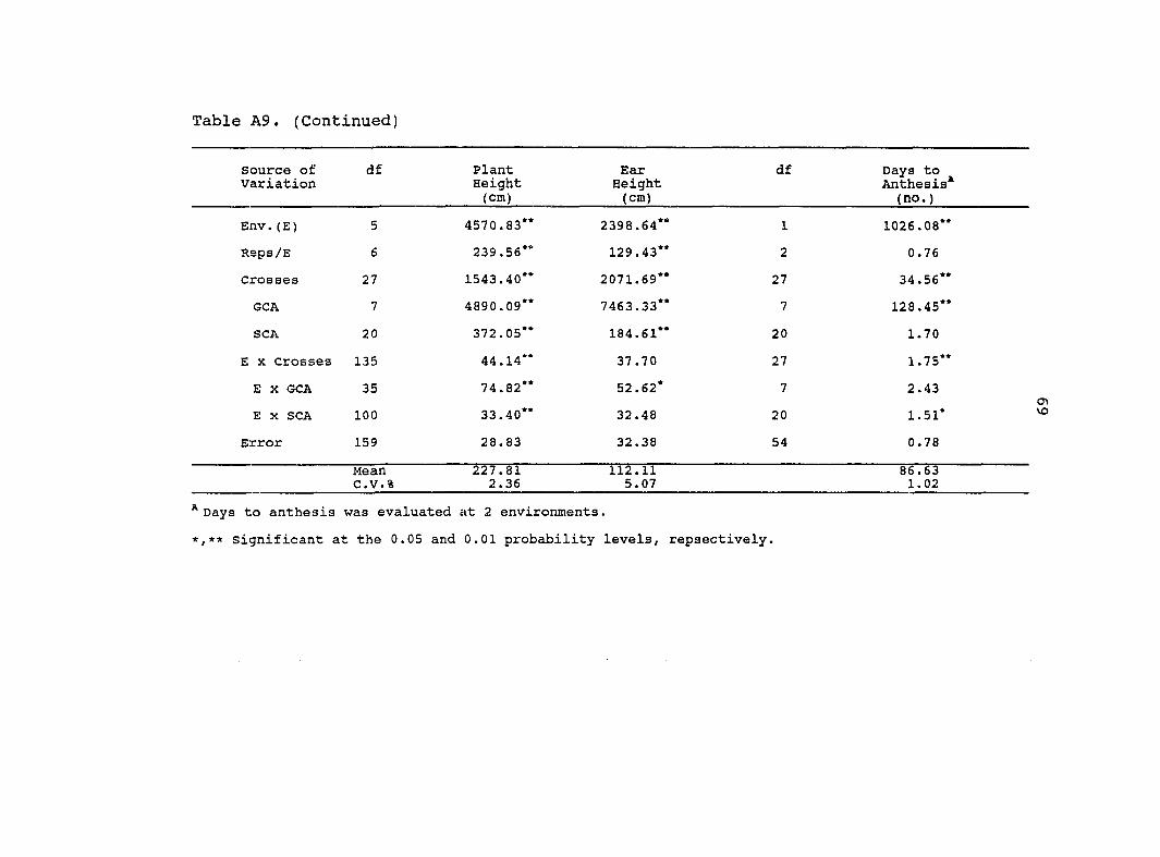
Table A9. (Continued)
source of Variation
df Plant Height (cm)
Ear Height (cm)
df Days to Anthesis* (no.)
Env.(E) 5 4570.83" 2398.64** 1 1026.08**
Reps/E 6 239.56** 129.43** 2 0.76
Crosses 27 1543.40** 2071.69** 27 34.56**
GCA 7 4890.09** 7463.33** 7 128.45**
SCA 20 372.05** 184.61** 20 1.70
E X Crosses 135 44.14** 37.70 27 1.75**
E X GCA 35 74.82** 52.62* 7 2.43
E X SCA 100 33.40** 32.48 20 1.51*
Error 159 28.83 32.38 54 0.78
Mean C.V.%
227.81 2.36
112.11 5.07
86.63 1.02
^ Days to anthesis was evaluated at 2 environments.
*,** significant at the 0.05 and 0.01 probability levels, repsectively.

Table AlO. Mean squares of the analysis of variance combined across 6 environments in 1993 & 1994 for set 10.
Source of Variation
df Grain Yield
(mg ha"^)
Grain Moisture (%)
Root Lodging (%)
Stalk Lodging (%)
Dropped Ears (%)
Env.(E) 5 235.25** 412.54** 37.07** 783.25** 17.68**
Reps/E 6 1.41** 13.92** 2.89 30.52 0.70
Crosses 27 12.80** 24.40** 6.04 245.22** 4.78**
GCA 7 42.75** 61.03** 12.08 680.21** 12.37**
SCA 20 2.32** 11.58** 3.92 92.98** 2.12
E X crosses 135 1.03** 3.64** 4.34 53.42** 1.81
E X GCA 35 2.15** 7.80** 7.52** 79.53* 2.10
E X SCA 100 0.64* 2.19 3.23 44.28** 1.71
Error 162 0.48 1.67 3.71 28.68 2.33
Mean c.v.%
6.93 9.96
25.33 5.10
0.73 263.83
10.64 50.33
0.69 221.42
*, ** significant at the 0.05 and 0.01 probability levels, respectively.

Table AlO. (Continued)
Source of Variation
df Plant Height (cm)
Ear Height (cm)
df Days to Anthesis* (no.)
Env.(E) 5 5193.82" 2724.02" 1 825.14**
Reps/E 6 188.53" 334.04" 2 3.95*
Crosses 27 2087.47" 1733.52" 27 10.24**
GCA 7 7116.78" 5850.23" 7 29.85**
SCA 20 327.22" 292.67" 20 3.38
E X Crosses 135 62.24" 33.51 27 1.75
E X GCA 35 95.31" 48.75* 7 2.00
E X SCA 100 50.67* 28.18 20 1.67
Error 162 34.01 21.64 54 1.06
Mean C.V.%
225.71 2.58
113.91 4.09
84.48 1.22
^Days to anthesis was evaluated at 2 environments.
*,** significant at the 0.05 and 0.01 probability levels, repsectively.

Table All. Mean squares of the analysis of variance combined across 6 environments in 1993 & 1994 for set 11.
Source of Variation
df Grain Yield
(mg ha~^)
Grain Moisture (%)
Root Lodging (%)
Stalk Lodging (%)
Dropped Ears (%)
Env.(E) 5 166.26** 598.23** 0.29** 663.29** 7.24**
Reps/E 6 1.39* 7.82** 0.54* 69.68 1.44
Crosses 27 3.41** 34.41** 0.80* 242.86** 5.10*
GCA 7 5.81 100.75** 1.02 687.59** 11.57*
SCA 20 2.57** 11.19** 0.72* 87.21** 2.84
E X Crosses 135 1.46** 4.00** 0.43** 37.23 2.75
E X GCA 35 2.32** 10.12** 0.49 60.43** 3.88**
E X SCA 100 1.16** 1.86 0.41** 29.10 2.35
Error 162 0.56 1.49 0.24 36.25 2.45
Mean C.v.%
6.23 12.04
25.02 4.87
0.11 444.28
9.78 61.56
0.57 274.85
*, ** significant at the 0.05 and 0.01 probability levels, respectively.

Table All. (Continued)
Source of Vairiation
df Plant Height (cm)
Ear Height (cm)
df Days to Anthesis* (no.)
Env.(E) 5 3974.86" 2109.52** 1 880.32**
Reps/E 6 229.79" 195.73** 2 11.18**
Crosses 27 1450.67" 1410.26** 27 12.99**
GCA 7 4844.80** 4594.13*' 7 36.17**
SCA 20 262.73** 295.90** 20 4.88**
E X Crosses 135 47.24 45.01* 27 0.77
E X GCA 35 92.56** 77.53** 7 1.10
E X SCA 100 31.38 33.62 20 0.65
Error 162 39.81 32.35 54 0.77
Mean C.V.%
223.71 2.82
111.61 5.10
86.30 1.02
^ Days to anthesis was evaluated at 2 environments.
*,** Significant at the 0.05 and 0.01 probability levels, repsectively.

Table A12. Mean squares of the analysis of variance combined across 6 environments in 1993 & 1994 for set 12.
source of Variation
df Grain Yield
(mg ha"^)
Grain Moisture (%)
Root Lodging (%)
Stalk Lodging (%)
Dropped Ears (%)
Env.(E) 5 215.97** 501.03** 107.65** 1643.43** 7.39**
Reps/E 6 0.81 5.14** 3.81 116.44 2.09
Crosses 27 6.18** 73.22** 55.87** 1149.95** 4.15**
GCA 7 11.01 234.38** 128.63 3731.78** 7.62
SCA 20 4.49** 16.81** 30.41* 246.31** 2.94
E X Crosses 135 1.20** 3.66** 19.16 132.43** 2.09
E X GCA 35 2.16** 8.13** 38.51** 212.39** 2.24
E X SCA 100 0.86** 2.09* 12.38 104.44** 2.04
Error 162 0.54 1.42 15.51 64.19 1.74
Mean c.v.%
5.62 13.08
24.51 4.87
1.42 277.32
16.96 47.24
0.48 274.62
*, ** significant at the 0.05 and 0.01 probability levels, respectively.

Table A12. (Continued)
Source of Variation
df Plant Height (cm)
Ear Height (cm)
df Days to Anthesis^ (no.)
Env.(E) 5 6748.84** 2904.59** 1 1026.08**
Reps/E 6 220.65** 117.12* 2 6.15**
Crosses 27 1622.83** 1240.22** 27 14.16**
GCA 7 4983.74** 3447.87** 7 48.33**
SCA 20 446.51** 467.54** 20 2.20*
E X Crosses 135 75.96 52.13 27 1.82**
E X GCA 35 124.69** 112.97** 7 3.97**
E X SCA 100 58.91 30.83 20 1.07
Error 162 78.62 52.29 54 0.73
Mean C.V.%
230.41 3.85
118.21 6.12
87.01 0.98
* Days to anthesis was evaluated at 2 environments.
*,** significant at the 0.05 and 0.01 probability levels, repsectively.
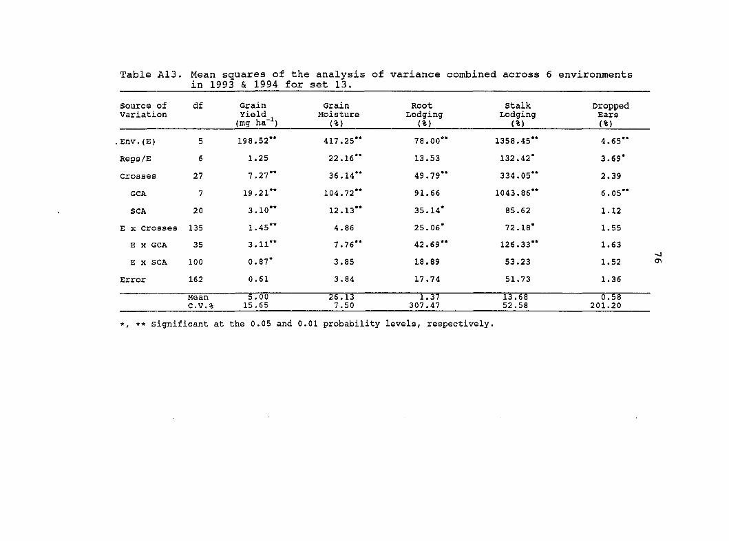
Table A13. Mean squares of the analysis of variance combined across 6 environments in 1993 & 1994 for set 13.
Source of Variation
df Grain Yield
(mg ha"^)
Grain Moisture (%)
Root Lodging (%)
Stalk Lodging (%)
Dropped Ears (%)
Env.(E) 5 198.52" 417.25" 78.00" 1358.45** 4.65**
Reps/E 6 1.25 22.16" 13.53 132.42* 3.69*
Crosses 27 7.27" 36.14" 49-79" 334.05** 2.39
GCA 7 19.21" 104.72" 91.66 1043.86** 6.05**
SCA 20 3.10" 12.13" 35.14* 85.62 1.12
E X crosses 135 1.45" 4.86 25.06* 72.18* 1.55
E X GCA 35 3.11" 7.76" 42.69** 126.33** 1.63
E X SCA 100 0.87* 3.85 18.89 53.23 1.52
Error 162 0,61 3.84 17.74 51.73 1.36
Mean c.v. %
5.00 15.65
26.13 7.50
1.37 307.47
13.68 52.58
0.58 201.20
*, ** significant at the 0.05 and 0.01 probability levels, respectively.
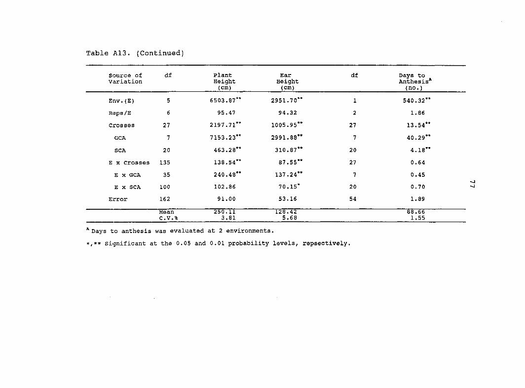
Table A13. (Continued)
source of Variation
df Plant Height (cm)
Ear Height (cm)
df Days to Anthesis^ (no.)
Env.(E) 5 6503.87" 2951.70" 1 540.32"
Reps/E 6 95.47 94.32 2 1.86
Crosses 27 2197.71" 1005.95" 27 13.54"
GCA 7 7153.23" 2991.88" 7 40.29"
SCA 20 463.28" 310.87" 20 4.18"
E X Crosses 135 138.54" 87.55" 27 0.64
E X GCA 35 240.48" 137.24" 7 0.45
E X SCA 100 102.86 70.15* 20 0.70
Error 162 91.00 53.16 54 1.89
Mean c.v.%
250.11 3.81
128.42 5.68
88.66 1.55
* Days to anthesis was evaluated at 2 environments.
*,** significant at the 0.05 and 0.01 probability levels, repsectively.

Table A14. Estimates of genetic components of variance^ (± SE) for yield, their interaction with the environment, the error variances, and the average level of dominance (d), combined across environments for the original diallel (set 1) and for each of the random diallels (sets 2-13).
S6t /t2 J " A " D " A G " D B " "
1 0.22 ± 0.16 0.53 ± 0.18 0.22 ± 0.06 0.14 ± 0.08 0.65 ± 0.07 2.19
2 -.07 ± 0.03 0.17 ± 0.06 0.43 ± 0.08 0.02 ± 0.05 0.46 ± 0.05
3 0.32 ± 0.14 0.15 ± 0.06 0.21 ± 0.05 -.03 ± 0.05 0.56 ± 0.06 0.97
4 0.24 ± 0.12 0.11 ± 0.06 0.34 ± 0.08 0.14 ± 0.07 0.55 ± 0.06 0.95
5 0.07 ± 0.06 0.15 ± 0.06 0.19 ± 0.05 0.04 ± 0.05 0.47 ± 0.05 2.07
6 -.05 ± 0.07 0.50 ± 0.17 0.23 ± 0.06 0.06 ± 0.07 0.65 ± 0.07
7 0.73 ± 0.30 0.15 ± 0.06 0.45 ± 0.09 0.09 ± 0.06 0.49 ± 0.05 0.64

Table A14. (Continued)
8 0.13 ± 0.09 0.29 ± 0.10 0.10 ± 0.03 0.13 ± 0.05 0.34 ± 0.04 2.11
9 0.16 ± 0.08 0.09 ± 0.05 0.12 ± 0.04 0.12 ± 0.07 0.53 ± 0.06 1.06
10 1.08 ± 0.40 0.14 ± 0.06 0.25 ± 0.06 0.08 ± 0.06 0.48 ± 0.05 0.51
11 0.06 ± 0.06 0.12 ± 0.07 0.19 ± 0.07 0.30 ± 0.09 0.56 ± 0.06 2.00
12 0.14 ± 0.11 0.30 ± 0.11 0.22 ± 0.06 0.16 ± 0.07 0.54 ± 0.06 2.07
13 0.38 ± S
0.18 0.18 ± 0.08 0.37 ± 0.09 0.13 ± 0.08 0.61 ± 0.07 0.97
O n , O j j , o a R / a n d O D B a r e t h e a d d i t i v e , d o m i n a n c e , a d d i t i v e b y e n v i r o n m e n t i n t e r a c t i o n , a n d Ominance by environment interaction components of variance, respectively.
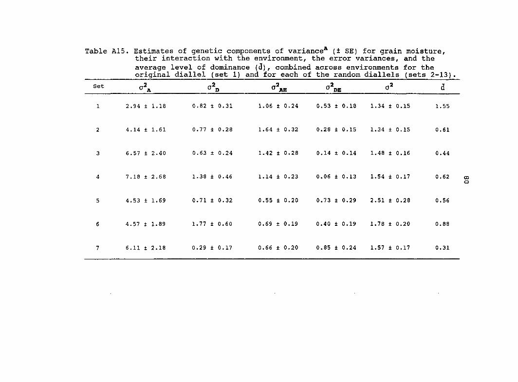
Table A15. Estimates of genetic components of variance^ (± SE) for grain moisture, their interaction with the environment, the error variances, and the average level of dominance (d), combined across environments for the original diallel (set 1) and for each of the random diallels (sets 2-13)
q^D
1 2.94 ± 1.18 0.82 ± 0.31 1.06 ± 0.24 0.53 ± 0.18 1.34 ± 0.15 1.55
2 4.14 ± 1.61 0.77 ± 0.28 1.64 ± 0.32 0.28 ± 0.15 1.34 ± 0.15 0.61
3 6.57 ± 2.40 0.63 ± 0.24 1.42 ± 0.28 0.14 ± 0.14 1.48 ± 0.16 0.44
4 7.18 ± 2.68 1.38 ± 0.46 1.14 ± 0.23 0.06 ± 0.13 1.54 ± 0.17 0.62
5 4.53 ± 1.69 0.71 ± 0.32 0.55 ± 0.20 0.73 ± 0.29 2.51 ± 0.28 0.56
6 4.57 ± 1.89 1.77 ± 0.60 0.69 ± 0.19 0.40 ± 0.19 1.78 ± 0.20 0.88
7 6.11 ± 2.18 0.29 ± 0.17 0.66 ± 0.20 0.85 ± 0.24 1.57 ± 0.17 0.31
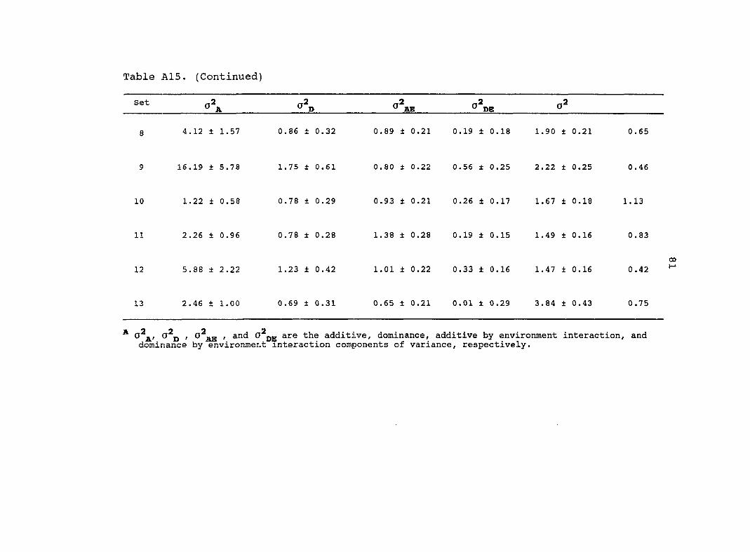
Table A15. (Continued)
8 4.12 ± 1.57 0.86 ± 0.32 0.89 ± 0.21 0.19 ±
CD
O 1.90 ± 0.21 0.65
9 16.19 ± 5.78 1.75 ± 0.61 0.80 ± 0.22 0.56 ± 0.25 2.22 ± 0.25 0.46
10 1.22 ± 0.58 0.78 ± 0.29 0.93 ± 0.21 0.26 ± 0.17 1.67 ± 0.18 1.13
11 2.26 ± 0.96 0.78 ± 0.28 1.38 ± 0.28 0.19 ± 0.15 1.49 ± 0.16 0.83
12 5.88 ± 2.22 1.23 ± 0.42 1.01 ± 0.22 0.33 ± 0.16 1.47 ± 0.16 0.42
13 2.46 ± 1.00 0.69 ± 0.31 0.65 ± 0.21 0.01 ± 0.29 3.84 ± 0.43 0.75
* 2 2 2 2 ̂ A.' D ' aw ' ̂D5 '''̂ ® additive, dominance, additive by environment interaction, and dominance by environment interaction components of variance, respectively.
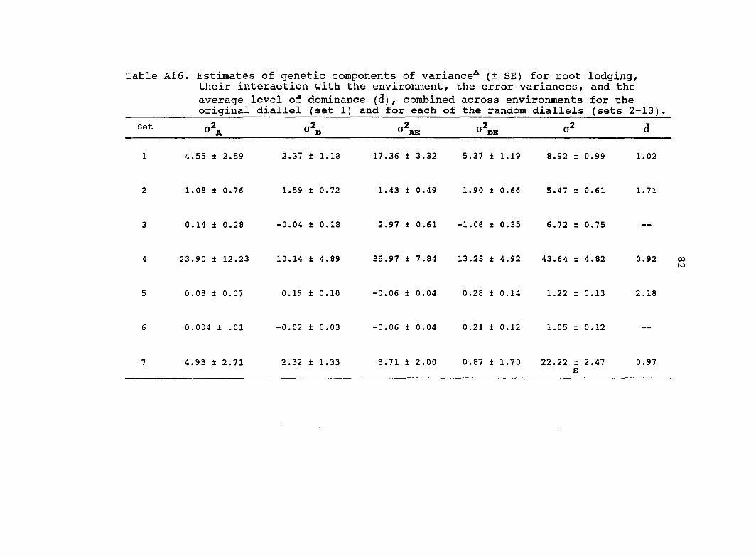
Table A16. Estimates of genetic components of variance^ (± SE) for root lodging, their interaction with the environment, the error variances, and the average level of dominance (d), combined across environments for the original diallel (set 1) and for each of the random diallels (sets 2-13).
^ g^DB <3
1 4.55 ± 2.59 2.37 ± 1.18 17.36 ± 3.32 5.37 ± 1.19 8.92 ± 0.99 1.02
2 1.08 ± 0.76 1.59 ± 0.72 1.43 ± 0.49 1.90 ± 0.66 5.47 ± 0.61 1.71
3 0.14 ± 0.28 -0.04 ± 0.18 2.97 ± 0.61 -1.06 i 0.35 6.72 ± 0.75
4 23.90 ± 12.23 10.14 ± 4.89 35.97 ± 7.84 13.23 ± 4.92 43.64 ± 4.82 0.92
5 0.08 ± 0.07 0.19 ± 0.10 -0.06 ± 0.04 0.28 ± 0.14 1.22 ± 0.13 2.18
6 0.004 ± .01 -0.02 ± 0.03 -0.06 ± 0.04 0.21 ± 0.12 1.05 ± 0.12
7 4.93 ± 2.71 2.32 ± 1.33 8.71 ± 2.00 0.87 ± 1.70 22.22 ± 2.47 0.97 s

Table A16. (Continued)
8 19.40 ± 9.45 12.48 ± 4.70 16.63 ± 3.74 3.37 ± 2.57 29.75 ± 3.30 1.13
9 19.60 ± 11.56 25.02 ± 9.18 19.45 ± 4.95 10.97 ± 4.48 41.91 ± 4 .63 1.60
10 0.11 ± 0.13 0.06 ± 0.10 0.71 ± 0.21 -0.24 ± 0.25 3.71 ± 0.41 1.04
11 0.006 ± 0.01 0.02 ± 0.02 0.01 ± 0.02 0.09 ± 0.04 0.24 ± 0.03 —
12 2.00 ± 1.26 1.50 ± 0.78 4.35 ± 1.06 -1.56 ± 0.89 15.51 ± 1.72 1.22
13 0.91 ± 0.94 1,35 ± 0.91 3.97 ± 1.17 0.57 ± 1.34 17.74 ± 1.97 1.72
& ^ 9 2 2 O *, O jj, O and O jjg are the additive, dominance, additive by environment interaction, and dominance by environment interaction components of variance, respectively.

Table A17. Estimates of genetic components of variance^ (± SE) for stalk lodging, their interaction with the environment, the error variances, and the average level of dominance (d), combined across environments for the original diallel (set 1) and for each of the random diallels (sets 2-13)
2! L_
1 52.96 ± 22.34 14.80 ± 6.67 28.84 ± 7.07 5.65 ± 5.96 73.61 ± 8.18 0.75
2 23.26 ± 11.42 10.14 ± 4.65 27.79 ± 6.25 3.25 ± 4.31 54.74 ± 6.04 0.93
3 83.34 ± 33.03 22.88 ± 8.72 22.29 ± 5.61 1.51 ± 4.97 67.74 ± 7.48 0.74
4 114.39 ± 43.72 16.55 ± 8.78 22.94 ± 7.73 29.56 ±„10.11 85.18 ± 9.40 0.54 s®
5 22.62 ± 8.99 4.91 ± 2.43 5.65 ± 1.93 1.97 ± 2.57 32.47 ± 3.58 0.66 s s
6 140.11 ± 51.67 20.68 ± 9.19 7.35 ± 4.32 16.10 ± 7.97 81.37 ± 8.98 0.54 S
7 106.36 ± 39.71 7.72 ± 6.34 17.26 ± 6.94 23.58 ± 10.49 102.51 ±11.32 0.38 S

Table A17. (Continued)
Sst Q2 _2 J " A " D " A B " D E ^ Q
8 34.74 ± 14.39 5.53 ± 3.84 17.45 ± 5.11 16.36 ± 5.74 49.03 ± 5.41 0.56 S
9 13.48 ± 6.96 6.47 ± 3.65 14.66 ± 4.18 14.04 ± 4.52 36.33 ± 4.01 0.98 s s
10 15.33 ± 6.54 4.06 ± 2.39 5.87 ± 2.18 7.80 ± 3.11 28.68 ± 3.17 0.73 s s s
11 15.81 ± 6.57 4.84 ± 2.22 5.22 ± 1.66 — 36.25 ± 4.00 0.78 s s
12 93.82 ± 35.44 11.82 ± 6.31 17.99 ± 5.82 20.12 ± 7.32 64.19 ± 7.09 0.50 S
13 24.59 ± 9.98 2.70 ± 2.24 12.18 ± 3.46 0.75 ± 3.75 51.73 ± 5.71 0.47
^ O^JJ, and O^jjg are the additive, dominance, additive by environment interaction, and Ominance by environment interaction components of variance, respectively.
® estimate is significantly different from set 1 estimate. All other estimates are not significantly different from set 1 unless indicated.
c estimates was zero or negative.

Table A18. Estimates of genetic components of variance^ (± SE) for dropped ears, their interaction with the environment, the error variances, and the average level of dominance (d) , combined across environments for the original diallel (set 1) and for each of the random diallels (sets 2-13)
Set ^2 ^2 J " A " D " A B ° D B ^ "
1 0.16 ± 0.08 0.07 ± 0.06 0.01 ± 0.05 -0.46 ± 0.13 2.41 ± 0.27 0.93
2 0.32 ± 0.19 0.21 ± 0.15 0.17 ± 0.12 0.47 ± 0.24 2.25 ± 0.25 1.14
3 0.64 ± 0.32 0.41 ± 0.24 0.06 ± 0.13 0.87 ± 0.32 2.63 ± 0.29 1.13
4 0.04 ± 0.02 -0.02 ± 0.02 0.04 ± 0.03 0.07 ± 0.08 0.79 ± 0.09
5 0.05 ± 0.03 0.06 ± 0.04 0.01 ± 0.02 -0.06 ± 0.07 0.85 ± 0.09 1.55
6 0.37 ± 0.16 -0.11 ± 0.06 0.16 ± 0.11 0.21 ± 0.23 2.64 ± 0.29
7 0.36 ± 0.21 0.32 ± 0.17 0.21 ± 0.11 -0.86 ± 0.23 4.48 ± 0.49 1.33

Table A18. (Continued)
Set A E D E
0.07 ± 0.05 0.04 ± 0.05 0.11 ± 0.06 0.06 ± 0.12 1.38 ± 0.15 1.07
0.26 ± 0.02 0.01 ± 0.03 0.02 ± 0.04 -0.08 ± 0.09 1.19 ± 0.13 0.27
10 0.27 ± 0.12 0.03 ± 0.06 0.06 ± 0.06 -0.31 ± 0.15 2.33 ± 0.26 0.47
11 0 . 2 0 ± 0 . 1 2 0.04 ± 0.08 0.25 ± 0.11 -0.05 ± 0.18 2.45 ± 0.27 0.63
12 0.12 ± 0.08 0 . 0 8 ± 0 . 0 8 0.03 ± 0.06 0.15 ± 0.16 1.74 ± 0.19 1.15
CO
13 0.13 ± 0.06 -0.03 ± 0.03 0.02 ± 0.05 0.08 ± 0.12 1.36 ± 0.15
* 2 2 0 2 O O jj, O and O jjg are the additive, dominance, additive by environment interaction, and ominance by environment interaction components of variance, respectively.

Table A19. Estimates of genetic components of variance^ (± SE) for plant height, their interaction with the environment, the error variances, and the average level of dominance (d), combined across environments for the original diallel (set 1) and for each of the random diallels (sets 2-13)
Set rj^ A
1 106.22 ± 39.45 21.45 ± 7.16 10.89 ± 2.53 1.67 ± 1.91 23.64 ± 2.63 0.63
2 161.17 ± 58.43 22.69 ± 7.61 13.80 ± 3.09 1.24 ± 2.12 27.57 ± 3.04 0.53
3 296.IQ ± 104.36 24.75 ± 8.50 6.02 ± 2.10 1.96 ± 2.86 36.65 ± 4.05 0.41
4 164.01 ± 58.47 15.20 ± 5.50 11.59 ± 2.89 2.45 ± 2.51 30.76 ± 3.40 0.43
5 476.47 ± 165.33 25.74 ± 9.03 2.01 ± 1.70 6.80 ± 3.50 36.17 ± 3.99 0.33
6 140.41 ± 54.09 48.06 ± 15.48 7.47 ± 2.29 4.62 ± 2.73 29.58 ± 3.27 0.83
7 178.35 ± 62.73 11.97 ± 4.66 6.40 ± 2.17 5.18 ± 2.87 30.44 ± 3.36 0.36
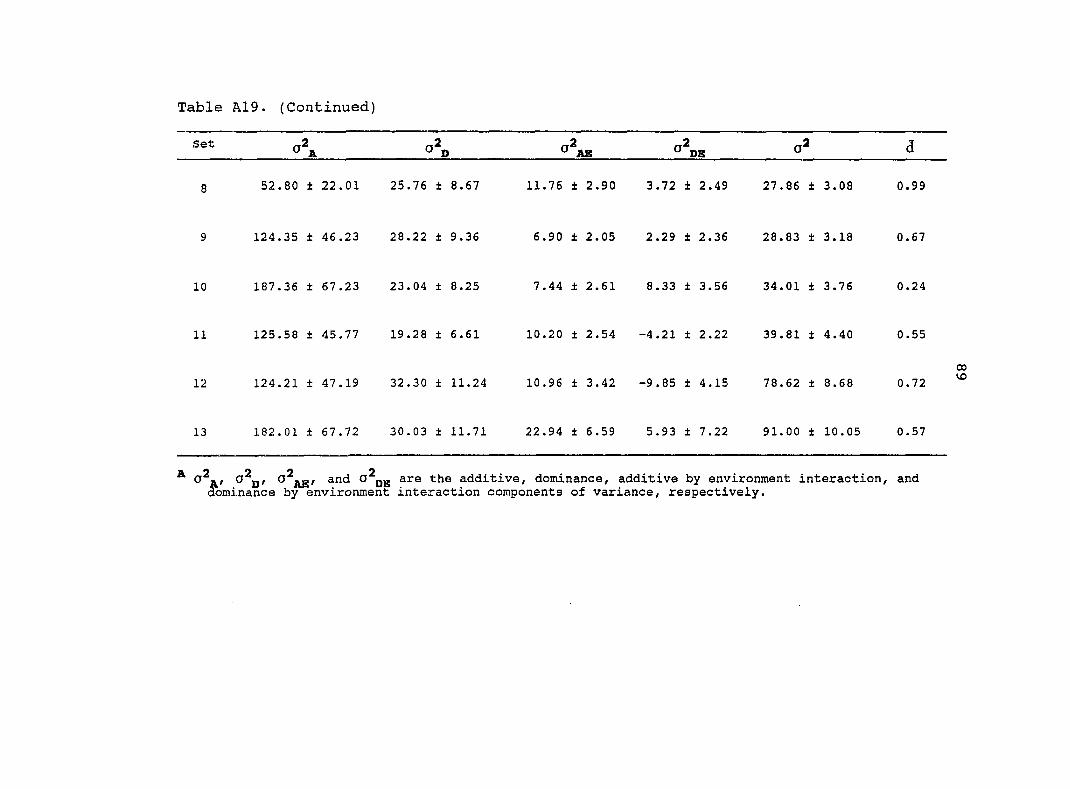
Table A19. (Continued)
^2 q2 qZ Q2 —2 ^ " A " D " A G " D B
9 52.80 ± 22.01 25.76 ± 8.67 11.76 ± 2.90 3.72 ± 2.49 27.86 ± 3.08 0.99
9 124.35 ± 46.23 28.22 ± 9.36 6.90 ± 2.05 2.29 ± 2.36 28.83 ± 3.18 0.67
10 187.36 ± 67.23 23.04 ± 8.25 7.44 ± 2.61 8.33 ± 3.56 34.01 ± 3.76 0.24
11 125.58 ± 45.77 19.28 ± 6.61 10.20 ± 2.54 -4.21 ± 2.22 39.81 ± 4.40 0.55
12 124.21 ± 47.19 32.30 ± 11.24 10.96 ± 3.42 -9.85 ± 4.15 78.62 ± 8.68 0.72
13 182.01 ± 67.72 30.03 ± 11.71 22.94 ± 6.59 5.93 ± 7.22 91.00 ± 10.05 0.57
^ additive, dominance, additive by environment interaction, and Ominance by environment interaction components of variance, respectively.

Table A20. Estimates of genetic components of variance^ (± SE) for ear height, their interaction with the environment, the error variances, and the average level of dominance (<3) , combined across environments for the original diallel (set 1) and for each of the random diallels (sets 2-13)
Set q2 Q2 Q2 J " A " D " A K " P B "
1 59.32 ± 21.72 7.35 ± 2.85 8.07 ± 2.01 2.34 ± 1.75 19.86 ± 2.21 0.50
2 50.34 ± 20.71 20.26 ± 6.91 15.79 ± 3.46 5.30 i 2.21 20.89 ± 2.31 0.90
3 228.61 ± 79.03 5.56 ± 2.38 8.69 ± 2.17 0.77 ± 1.90 25.40 ± 2.80 0.22
4 316.91 ± 109.93 12.07 ± 4.89 7.71 ± 2.60 0.25 ± 3.41 47.85 ± 5.28 0.28
5 333.33 ± 115.60 15.94 ± 5.97 2.32 ± 1.63 8.72 ± 3.20 28.08 ± 3.10 0.31
6 107.76 ± 39.90 23.24 ± 7.71 5.85 ± 1.72 2.41 ± 1.94 22.72 i 2.51 0.66
7 138.72 ± 48.40 7.58 ± 3.18 0.91 ± 1.10 2.18 ± 2.44 30.20 ± 3.33 0.33

Table A20. (Continued)
Set AB O" D B
82.92 ± 30.77 16.08 ± 5.54 8.28 ± 2.11 2.93 ± 1.92 21.31 ± 2.35 0.62
201.63 ± 70.44 12.68 ± 4.65 3.36 ± 1.44 0.05 ± 2.29 32.38 ± 3.57 0.35
10 153.80 ± 55.24 22.04 ± 7.36 3.43 ± 1.34 3.27 ± 1.99 21.64 ± 2.39 0.53
11 118.17 ± 43.42 21.86 ± 7.45 7.32 ± 2.13 0.64 ± 2.37 32.35 ± 12.76 0.61
12 80.50 ± 32.70 36.39 ± 11.76 13.69 ± 3.10 -10.73 ± 2.19 52.29 ± 5.77 0.95
13 72.61 ± 28.42 26.06 ± 7.86 11.18 ± 3.76 8.49 ± 4.93 53.16 ± 5.87 0.86
9 5 9 2 O a / O p , O j j g , a n d O j j g a r e t h e a d d i t i v e , d o m i n a n c e , a d d i t i v e b y e n v i r o n m e n t i n t e r a c t i o n , a n d ^minance by environment interaction components of variance, respectively.

Table A21. Estimates of genetic components of variance^ (± SE) for days to anthesis height, their interaction with the environment, the error variances, and the average level of dominance (d), combined across environments for the original diallel (set 1) and for each of the random diallels (sets 2-13).
o^D £^*5 ^ 3
1 1.04 ± 0.46 0.28 ± 0.23 0.11 ± 0.13 0.14 ± 0.26 1.27 ± 0.24 0.73
2 3.39 ± 1.30 0.15 ± 0.44 0.10 ± 0.25 0.03 ± 0.63 3.73 ± 1.00 0.30
3 0.94 ± 0.50 0.09 ± 0.16 0.64 ± 0.29 0.35 ± 0.21 0.63 ± 0.12 0.44
4 2.04 ± 0.70 -0.12 ± 0.12 -0.07 ± 0.06 0.22 ± 0.22 0.89 ± 0.17 ~
5 2.88 ± 1.04 0.33 ± 0.20 -.003 ± 0.07 0.25 ± 0.19 0.64 ± 0.12 0.48
6 3.13 ± 1.19 0.57 ± 0.29 0.19 ± 0.14 0.41 ± 0.22 0.54 ± 0.10 0.60
7 0.24 ± 0.18 0.19 ± 0.28 -0.07 ± 0.17 0.62 ± 0.35 0.97 ± 0.18 1.26
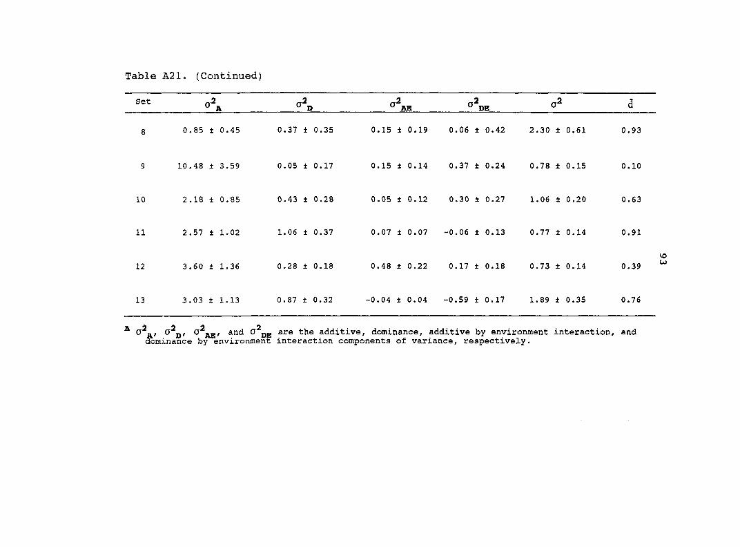
Table A21. (Continued)
Set o' Ag D B
0.85 ± 0.45 0.37 ± 0.35 0.15 ± 0.19 0.06 ± 0.42 2.30 ± 0.61 0.93
10.48 ± 3.59 0.05 ± 0.17 0.15 ± 0.14 0.37 ± 0.24 0.78 ± 0.15 0.10
10 2.18 ± 0.85 0.43 ± 0.28 0.05 ± 0.12 0.30 ± 0.27 1.06 ± 0.20 0.63
11 2.57 ± 1.02 1.06 ± 0.37 0.07 ± 0.07 -0.06 ± 0.13 0.77 ± 0.14 0.91
12 3.60 ± 1.36 0.28 ± 0.18 0.48 ± 0.22 0.17 ± 0.18 0.73 ± 0.14 0.39 U)
13 3.03 ± 1.13 0.87 ± 0.32 -0.04 ± 0.04 -0.59 ± 0.17 1.89 ± 0.35 0.76
CF _, O jj, O ag/ and O jjg are the additive, dominance, additive by environment interaction, and dominance by environment interaction components of variance, respectively.

94
Table A22. Trait means for the original diallel and the 12 pooled random diallels combined across six environments in 1993 & 1994.
Trait* Diallel Mean
Grain Yield (Mg ha"^)
Original Random®
6.48 5.98
Grain Moisture (g kg"^)
Original Random
25.11 24.28
Root Lodging (%)
Original Random
2 . 1 2 1 . 6 2
Stalk Lodging (%)
Original Random
18.31 15.69
Dropped Ears (%)
Original Random
0.67 0.63
Plant Height (cm)
Ear Height (cm)
Original Random
Original Random
245.10 227.89
129.90 116.78
Days to anthesis (#)
Original Random
8 8 . 1 8 86.43
* All traits were evaluated in six environments except Days to anthesis which was evaluated in two environments.
® Pooled random diallels.
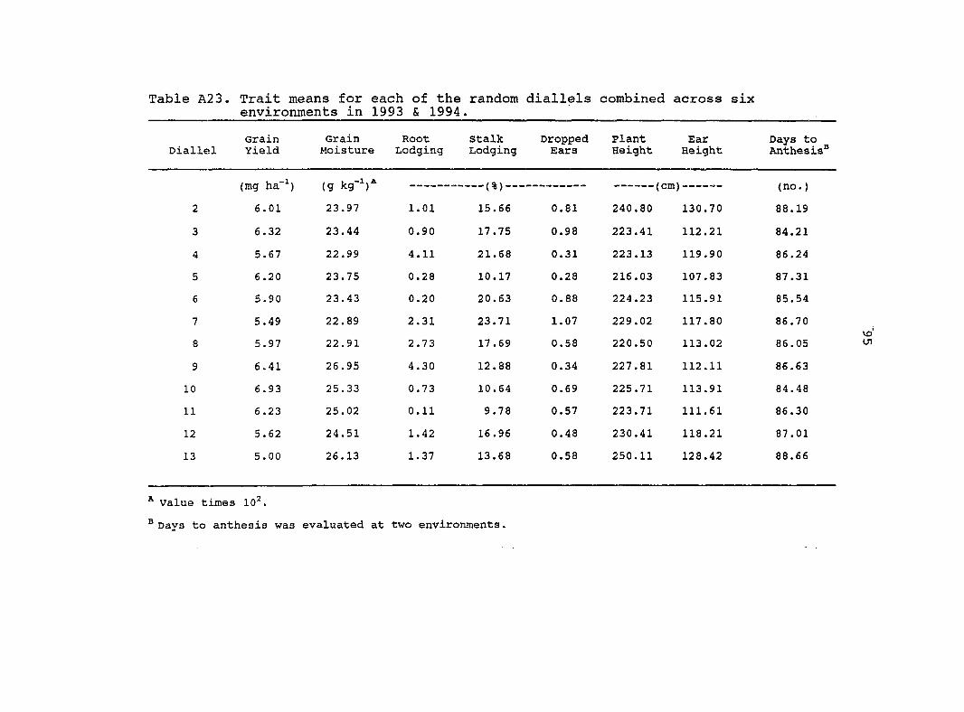
Table A23. Trait means for each of the random diallels combined across six environments in 1993 & 1994.
Grain Grain Root stalk Dropped Plant Ear Days to Diallel Yield Moisture Lodging Lodging Ears Height Height Anthesis®
(mg ha (g kg-̂ )"" (no.) (mg ha (g kg-̂ )"" ( «) (cm) •- (no.)
2 6.01 23.97 1.01 15.66 0.81 240.80 130.70 88.19
3 6.32 23.44 0.90 17.75 0.98 223.41 112.21 84.21
4 5.67 22.99 4.11 21.68 0.31 223.13 119,90 86.24
5 6.20 23.75 0.28 10.17 0.28 216.03 107.83 87.31
6 5.90 23.43 0.20 20.63 0.88 224.23 115.91 85.54
7 5.49 22.89 2.31 23.71 1.07 229.02 117.80 86.70
8 5.97 22.91 2.73 17.69 0.58 220.50 113.02 86.05
9 6.41 26.95 4.30 12.88 0.34 227.81 112.11 86.63
10 6.93 25.33 0.73 10.64 0.69 225.71 113.91 84.48
11 6.23 25.02 0.11 9.78 0.57 223.71 111.61 86.30
12 5.62 24.51 1.42 16.96 0.48 230.41 118.21 87.01
13 5.00 26.13 1.37 13.68 0.58 250.11 128.42 88.66
* value times 10^.
® Days to anthesis was evaluated at two environments.