propensities and probabilities - university of...
TRANSCRIPT

ARTICLE IN PRESS
Studies in History and Philosophy of
Modern Physics 38 (2007) 593–625
1355-2198/$ -
doi:10.1016/j
E-mail ad
www.elsevier.com/locate/shpsb
Propensities and probabilities
Nuel Belnap
1028-A Cathedral of Learning, University of Pittsburgh, Pittsburgh, PA 15260, USA
Received 19 May 2006; accepted 6 September 2006
Abstract
Popper’s introduction of ‘‘propensity’’ was intended to provide a solid conceptual foundation for
objective single-case probabilities. By considering the partly opposed contributions of Humphreys
and Miller and Salmon, it is argued that when properly understood, propensities can in fact be
understood as objective single-case causal probabilities of transitions between concrete events. The
chief claim is that propensities are well-explicated by describing how they fit into the existing formal
theory of branching space-times, which is simultaneously indeterministic and causal. Several
problematic examples, some commonsense and some quantum-mechanical, are used to make clear
the advantages of invoking branching space-times theory in coming to understand propensities.
r 2007 Elsevier Ltd. All rights reserved.
Keywords: Propensities; Probabilities; Space-times; Originating causes; Indeterminism; Branching histories
1. Introduction
You are flipping a fair coin fairly. You ascribe a probability to a single case by asserting
The probability that heads will occur on this very next flip is
about 50%. ð1Þ
The rough idea of a single-case probability seems clear enough when one is told that thecontrast is with either generalizations or frequencies attributed to populations assertedwhile you are flipping a fair coin fairly, such as
In the long run; the probability of heads occurring among flips is about 50%.
ð2Þ
see front matter r 2007 Elsevier Ltd. All rights reserved.
.shpsb.2006.09.003
dress: [email protected]
ARTICLE IN PRESSN. Belnap / Studies in History and Philosophy of Modern Physics 38 (2007) 593–625594
Once one begins to study probability theory, however, one rapidly loses ones grip on whatit could mean to fasten a probability on an isolated case without thinking of it as part of agroup of similar cases—perhaps stretching over time and space. The reason is that thefrequency interpretation of probability, which is not only as venerable as, but also asattractive as, a California grandmother fresh from the spa, gives a kind of theoreticalsupport for the doctrine of the meaningless of single-case ascriptions of probability, since itspeaks always of the relative size of sets, and never of the single case. Popper (1959)articulates and defends the intelligibility of single-case ascriptions. After criticizing thefrequency interpretation in well-known ways that I shall not describe, Popper thought touse the idea of a propensity to make sense out of applying probabilities to the single case,whereas starting with Humphreys (1985), a number of philosophers have argued in theirturn that talk of propensities has not been justified, and in particular that conditionalprobabilities cannot be construed as propensities. As kind of a third party, I am going toparticipate in the dispute over propensity theory: I will be defending the idea of identifyingpropensities in the single case as causal probabilities in the sharply defined sense ofbranching space-times with probabilities (BSTP).1 The way in which I am going to mountthis defense is by showing, eventually, how a concept of propensities derivable from theliterature fits exactly into the theory of BSTP. Before I get to that, however, I will belooking at some of the discussion as it has emerged.My plan is this. In Section 2, I try to make clear the topic by offering as clear a
description as I can manage of earlier discussions of propensities as derived from Popper,emphasizing the variety of sometimes incompatible features that have been attributed tothem. Then in Section 3, I describe the little bit of probability theory that the discussionrequires, and with this as background, in Section 4, I discuss what has come to be knownas ‘‘Humphreys’s Paradox’’ by means of Humphreys’s own examples. In the course ofpresenting his objection to propensity theory, Humphreys introduces some notation forputative propensities; I discuss this new notation in Section 5. Miller (1994, 2002) uses thenew notation in order to defend the identification of propensities as probabilities, adevelopment some of the details of which I critique in Section 6. With that out of the way,I appear to come to the same conclusion as Miller, my argument of Section 7 depending ona tinker with one of Humphreys’s principle examples. Up to this point there has been agreat deal of informal argument by all parties. At last I review some key ideas of BSTP, anaxiomatic theory, in Section 8, and then in Section 9, I apply BSTP to yet anotherpropensity story (better: an anti-(propensity ¼ probability) story), a story due to Salmon.I suggest that the idea of a propensity is illuminated by identifying propensities with certaincausal probabilities—the probabilities of ‘‘causae causantes’’—in BSTP theory, a theorygoverned by rigorous definitions and axiomatic principles (no informality). Finally Isummarize and review conclusions in Section 10.
2. What is a propensity?
This is the place in this essay where I offer a preliminary idea of propensities. Since for‘‘propensity’’ no crisp understanding (much less a definition) is available, I assume the
1BSTP is explored in the following papers listed as references: Belnap (1992, 2003a) (BST), Belnap, Perloff, &
Xu (2001) (FF), Belnap (2002a) (DTR), Belnap (2002b)(FBBST), Belnap (2003a; 2003b)(NCCFB), Belnap
(2005a; 2005b) (CC), Muller (2002, 2005), Placek (2000a, 2000b).

ARTICLE IN PRESSN. Belnap / Studies in History and Philosophy of Modern Physics 38 (2007) 593–625 595
privilege of directing your attention by listing some loosely characterized features that, invarious combinations, have been attributed to propensities. In the end we should have atheoretically sharp account of propensities so we can relate them to single-case causalprobabilities, but for the present we have to live with looseness.
1.
Popper (1959, p. 68) explains a propensity as ‘‘the probability of the result of a singleexperiment, with respect to its conditions.’’ The rider, ‘‘with respect to its conditions,’’seems essential, but at best the meaning of that phrase is murky. Propensities are takenas characterizing ‘‘the whole physical situation,’’ a phrase that also clouds the mind.On the preceding page Popper says that ‘‘Every experimental arrangement is liable toproduce, if we repeat the experiment very often, a sequence with frequencies whichdepend upon this particular experimental arrangement.’’ It is evident that there is nosuggestion here of fastening a probability-of-occurrence onto the experiment itself;hence, in harmony with Humphreys, classical conditional probability is the wrongtool.If we take ‘‘single experiment’’ seriously, uniqueness is implied. Each experiment hasthe conditions that it has. Therefore, as long as we identify the experiment by itsspatio-temporal location as well as in terms of all the possible histories with which it isconsistent, ‘‘its conditions’’ are uniquely determined by the experiment itself.(‘‘Histories’’ is a technical term in BSTP, with a precise definition.) The phrase ‘‘withrespect to its conditions’’ might be thought redundant, and it might be thought that thephrase ‘‘the whole physical situation’’ calls for the same treatment: BSTP sees adifference here. (1) If ‘‘conditions’’ are in the past, then, as long as we do not waffle,conditions of a single experiment are unique, whether known or not. But (2) thephrase, ‘‘the whole physical situation,’’ leaves room for alternate possibilities. BSTPsays that if heads come up on a coin-toss, part of the actual total situation is that itmight have come up tails. (Possibilities are intraworldly in BSTP theory—see Section8.1—not other-worldly as in Lewis’s account.)
2.
Popper (1959, p. 37) also characterizes propensities as dispositional properties ofsingular events. Generally dispositions are taken to characterize enduring objects, butthat is not appropriate here (the idea is too complicated for an elementary discussion).At this point we want to think about something simpler: the disposition of a singularevent to be followed by events of a certain character. Propensities and dispositions, inthe required sense, are valenced toward the future (p. 36).
3.
That propensities explain probabilities is an appealing notion that lies behind a greatdeal of thought about them. This species of explanation in this case, however, shouldvividly remind you of the ‘‘dormative powers of opium’’ as a putative explanation ofwhy opium puts one to sleep.4.
Propensities for Popper are unashamedly indeterminist, since they ‘‘influence futuresituations without determining them.’’ There being a propensity for such and such maymake it likely, but is never a guarantee. That idea suits BSTP.5.
Propensities are objectives (p. 32). Subjective probability theory need not apply. 6. Propensities always, or for the most part, create a time-asymmetric situation. One yearLance Armstrong had a propensity to win the Tour de France the next year; but afterwinning that second year, he does not have a propensity for having won the Tour thefirst year. Pure probability theory is incapable of making the distinction. You have tohave become clear on indeterminist tense logic to appreciate Prior’s (1957) surprising

ARTICLE IN PRESSN. Belnap / Studies in History and Philosophy of Modern Physics 38 (2007) 593–625596
point that this temporal asymmetry nevertheless effortlessly allows that in early 2005,Lance Armstrong had a propensity to have been born a seven-time winner of the Tour
de France. See FF, p. 243, for the short version, and DTR for the long.
7. ‘‘Having a propensity. . .’’ can be used in perfectly idiomatic English to describepersons, animals, or non-living things (enduring objects), or even characteristics.Examples: ‘‘Angry folks have a propensity to act irrationally.’’ Put abstractly, ‘‘Angerhas a propensity to lead to violence.’’ Also ‘‘Dogs have a propensity to bite the handthat feeds them,’’ and ‘‘The jar on the left has a propensity to leak.’’ Also ‘‘Thisexperimental coin-flipping set-up has more of a propensity to produce heads than itdoes to produce tails.’’‘‘Having a propensity. . .’’ can also describe actions or events, especially in general-izations such as ‘‘Taking a pepper spray when setting out to walk the streets of NewYork has a propensity to lengthen your life,’’ or ‘‘Measuring coffee grounds accuratelyhas a propensity to result in a cheerful breakfast.’’These uses of ‘‘propensity’’ in generalizations flow easily. It is not so idiomatic tocharacterize a particular singular event as having a propensity unless one surroundsthe use with considerable context. ‘‘I understand that you are going walking on WallStreet first thing in the morning. I suggest that you see to it that you take a pepperspray. That action, should you carry it out, would have a propensity to lengthen yourlife.’’ Atheoretical philosophers often or always take the use of ‘‘propensity’’ or‘‘disposition’’ in generalizations as primary, or even exclusively intelligible. I believethat one cannot have a satisfactory theory of generalizations if one has nounderstanding of individual cases; for this reason, I am ignoring the frequentawkwardness of attributing a propensity in a single case. In this study I shall assumethat when we have our theories straight, we can always find some language that is goodenough to warrant application of propensities to singular events.
8.
Propensities come in degrees of more or less, high or low, etc. In the commonsense situations in which we speak of them, we hardly ever assign them numericaldegrees. In this respect, as well as many others, propensities resemble probabilities. Thatobservation encourages us to look for a way to bring probability theory to bear on
propensities.
9. If you have the possibility of carrying out one of several actions, you may have acertain propensity for more than one, or even for each. For instance, ‘‘Last night,before bed, I was trying to decide whether to have apple juice or orange juice. Because,however, my propensity for apple juice was the same as my propensity for orange juice,I gave up the internal debate in favor of making myself a chocolate milkshake.’’ Insuch cases, in spite of linguistic temptation, we should not identify ‘‘having a propensityfor’’ with ‘‘having some propensity for,’’ just as we refrain from confusing ‘‘beingprobable that’’ with ‘‘There is some probability that.’’ In this respect, too, propensitiesare much like probabilities.
10.
Gillies (2000) recommends saving ‘‘propensity theory’’ for ‘‘any theory which tries todevelop an objective, but non-frequency, interpretation of probability’’ (p. 808). Gillieseventually suggests that there are two kinds of propensity theories: long-run propensitytheories and single-case propensity theories. Gillies plumps for the former. His chiefargument against the latter is that they are ‘‘metaphysical’’ in a pejorative sense sincespeculations concerning them in their non-repeatable glory ‘‘cannot be tested againstdata’’ (p. 824). It is against this line that Popper is protesting in (1) above. What is
ARTICLE IN PRESSN. Belnap / Studies in History and Philosophy of Modern Physics 38 (2007) 593–625 597
non-repeatable is the event to which the propensity is attached, but this does not standin the way of taking the singular event to be of a certain repeatable kind that can wellbe involved in universal (law-like) generalizations. For a homely example, to say that acertain coin is fair can be taken to say that each and every flipping of the coin is fair.One cannot, of course, use the finite amount of evidence at one’s disposal to fashion adeductive argument to the conclusion that a particular toss (or sequence of tosses) wasfair. But that is just the same-old of scientific methodology.
11.
There is always some causal claim involved in an ascription of propensity. Salmon (1989)writes as follows:Propensities, I suggest, are best understood as some sort of probabilistic causes.
Presence or absence of causality stands as the enormous gap between a mere probabilityand a propensity. That is a repeated theme of most of the literature, and of this essay. Inthe theory of causation of Belnap (2005b), causation is analyzed in such a way as to requirethe underlying idea of concrete transitions (see von Wright, 1963), that is, transitions fromevent to event; which is another theme that I shall eventually exploit.
So much for some not-necessarily coherent abstract characterizations of propensities.There will be more about some of them, but first let us think about standard probabilities.
3. Probability theory
The ‘‘explanatory question’’ is, Do propensities explain probabilities? As I indicated in (3)above, I fail to be enamored of the suggestion that they do. The ‘‘identity question’’ is this:Are propensities probabilities? Having skimmed various characterizations of propensities,let us turn to probabilities in order to sharpen the question. For definiteness, I sketch hererudiments of Kolmogorov probability theory, emphasizing those few parts that are of usein understanding the debate about propensities, just to be sure that we are all talking thesame language.
A probability space is a triple hZ;F ;Pi; where Z is a non-empty
and finite ‘‘sample space,’’F is the boolean algebra of all subsets
of Z; P is a function from F into the interval ½0; 1�; Pð;Þ ¼ 0,
PðZÞ ¼ 1; and for all A;B 2 F ; if A \ B ¼ ; then PðA [ BÞ
¼ PðAÞ þ PðBÞ. ð3Þ
The definition does not allow for infinite probability spaces. As far as the discussion goesin this essay, finitude suffices to illustrate the crucial points.
Users of this calculus are generally happy to call each A 2 F (so that according to (3) A
is formally a set), an ‘‘event,’’ or perhaps a ‘‘proposition,’’ or to speak of the members of A
as events, and in either case to help themselves informally to the language of occurrence,often tensed. Thinking of A as a property, it is common to speak using (1) ‘‘A occurred fivetimes,’’ or (2) ‘‘five instances of A occurred,’’ or (3) various nominalizations such as ‘‘someof the occurrences of A will be occurrences of B’’, or (4) ‘‘the chances that A will occur.’’Readers accustomed to such usages should explicitly keep in mind that I shall reserve‘‘event’’ for certain concrete occupants of our world, which may actually occur, but also

ARTICLE IN PRESSN. Belnap / Studies in History and Philosophy of Modern Physics 38 (2007) 593–625598
may only possibly occur.2 The dominating association is with Lewis, who persuasivelydescribes the difference between the actual and the possible as perspectival rather thanintrinsic. (The fundamental difference from Lewis is that BSTP postulates just one world;see Section 8.2.)An event in BSTP theory, whether possible or actual, is as concrete as a Los Angeles
freeway. I also say (in adjectival form) of an event e that it may ‘‘possibly occur’’; that is ashort form for the more properly tensed form ‘‘e is occurring or did occur or will occur, ormight be occurring or might have occurred or might occur’’; and even that litany leaves outevents that are space-like related to me, which have the feature that it might be that theyhave occurred. Sometimes I use ‘‘possible event’’ with exactly the same meaning. It iscritical that every possible event is in a perhaps complicated space-time-like causal relationto me-here-now. I have in mind the ancestral of ‘‘either e1 is in the causal past of e2, or viceversa.’’ So as not to lengthen this essay unduly, I ask that you consult the BST papers ifyou wish a rigorous and I trust persuasive explanation.For our purposes, the most significant defined concept of probability theory is that of
‘‘conditional probability’’:
PðAjBÞ¼df
PðA \ BÞ
PðBÞ, (4)
where A \ B is set intersection and B is presumed non-empty. (Here and everywhere weignore the awkwardness of keeping track of division by zero.) There are many proposedEnglish readings of PðAjBÞ. Here is one found on the net:
PðAjBÞ is to be read in English as ‘‘the probability that A will
occur given that B has occurred :’’ ð5Þ
Those tangled tenses are at best difficult to penetrate. To avoid the complications of tense(by no means always a commendable aim), the following generic reading would appeal tomany:
the probability of A given B. (6)
For practical application, it often does not matter how you read conditional probability insloppy old English; that is the nature of atheoretical practicality. The tensed Englishreading (5) just will not matter in the thick of scientific discovery or testing.It is often good informal practice, because safest, to think of PðAjBÞ as the probability
PðAÞ of A with respect to the probability space obtained from the entire sample space, Z,of (3) by reducing Z to just its subset B. That is accurate, but hard to read. No wonder thefrequency interpretation is so attractive! On that interpretation, in the simplest casesPðAjBÞ is simply the proportion of A’s among the B’s as given by (4).Argle-bargle aside, the formal feature of the probability calculus on which Humphreys
(1985) rests his argument for the thesis (9) below that ‘‘propensities cannot beprobabilities’’ is that in its theory of conditional probability, the probability calculuspermits a Bayes-like inversion of condition and conditioned. ‘‘Inversion’’ does not, ofcourse, mean that PðAjBÞ ¼ PðBjAÞ; ‘‘Inversion’’ means only that PðAjBÞ and PðBjAÞ areequally grammatical and understandable. Perhaps the simplest theorem of the probability
2This is spelled out in detail in publications listed as references that are authored by any of the following:
Belnap, Perloff, Xu, Weinstein, Muller, and Placek.
ARTICLE IN PRESSN. Belnap / Studies in History and Philosophy of Modern Physics 38 (2007) 593–625 599
calculus exhibiting such an inversion is this:
PðAjBÞ �PðBÞ
PðAÞ¼ PðBjAÞ. (7)
This is a consequence of taking (4) as the definition of conditional probability in terms ofabsolute probabilities. It is more persuasive (?), however, to follow Popper in restrictingthe language of the abstract theory by omitting absolute probability terms such as ‘‘PðAÞ,’’taking as well-formed only notation for conditional probabilities ‘‘PðAjBÞ.’’ In that case,we have Bayes’s own theorem, which involves an inversion without invoking absoluteprobabilities:
PðBjðA \ CÞÞ ¼PðAjðB \ CÞÞ � PðBjCÞ
ðPðAjðB \ CÞ � PðBjCÞÞ þ ðPðAjðB \ CÞÞ � PðB \ CÞÞ. (8)
I am using the overline here as the sign of set complementation relative to the sample spaceZ of (3). The thing to note is that on the left of (8) there is ðBjAÞ (with ‘‘\C’’ as extracontext), while in the first upper term on the right there is the inversion ðAjBÞ (also with‘‘\C’’ as extra context). And that is enough or more than enough probability theory.
4. Humphreys’s Paradox
Now that we have our propensities and probabilities (Sections 2 and 3), we must dealwith Humphreys (1985), which initiated discussions of the relations between the two.Humphrey uses ‘‘chance’’ for an objective phenomenon to be contrasted with degrees ofrational belief or confirmation. For a perhaps contentious reason, I avoid this use of‘‘chance’’: The usage so often serves as a bludgeon with which to flatten an incompatibilistwithout responsible argument. My own view, expressed for example in FF, is indeedcompatibilist, but moves in the polar opposite direction: I take it that agency presupposesindeterminism, but not ‘‘chances’’ in the everyday sense that connotes mindlessness, or atleast lack of deliberation. The New Compatibilism, which, as a co-author of FF, I espouse,identifies a minimal sense of indeterminism that does not involve contrast with such heavyideas as ‘‘laws’’ or ‘‘scientific theories.’’ Minimal indeterminism is the doctrine that thereare occasions in this world of ours on which there is more than one alternative for thefuture, and that an occasion of deliberation is a paradigm example.
Putting aside the word, ‘‘chances,’’ Humphreys argues that probability theory in itspresent form cannot serve as a true theory of propensities. His essay was clearly the first torecognize problems in understanding propensities in terms of probabilities, putting hisconclusion with a provocatively crisp thesis:
Propensities cannot be probabilities. (9)
Humphreys always has in mind that propensities are conditional, so that propensitiesare usefully symbolized by prðAjBÞ, in contrast with standard conditional probabilities,written in the standard notation of probability theory as PðAjBÞ. Conditional propensitiesare tied to English by Humphreys with the equivalence,
prðAjBÞ is ‘‘the propensity for A to occur, conditional on the
occurrence of B’’ ðp: 560Þ. ð10Þ

ARTICLE IN PRESSN. Belnap / Studies in History and Philosophy of Modern Physics 38 (2007) 593–625600
As noted in Section 3, conditional probabilities, in standard probability theory, aregenerally given the English reading, (6) ‘‘the probability of A, given B,’’ and virtuallyalways interdefinable with absolute probabilities, either via (4) when absolute probabilitiesare primitive, or via PðAÞ¼df PðAjTautologyÞ if conditional probability expressions areprimitive. Do note that PðBÞ is, in either case, an absolute (unconditional) probability,which must certainly be a horse of an altogether different color.Humphrey’s principal lemma for (9) is that Bayes theorem fails for propensities. I should
not even need to remind you of Bayes theorem here, for the following reason: Argumentsagainst it are ‘‘so clearly directed against inversion principles that any considerationsinvolving other parts of the calculus seemed to be quite separate’’ (p. 567). This is a bigclaim since it calls into question either the much-worked-over foundations of appliedprobability theory or the intelligibility of the idea of a propensity. Humphreys’s (2004)brief article on Salmon reports that even after many, many years of conversations betweenthe pair, Humphreys himself believes that he and Salmon were divided on propensities.Humphreys thinks of Salmon as more attracted to frequencies than to propensities.3
Humphrey’s own belief is that
it is causal relevance that is important for single-case propensities,
not statistical relevance. ð11Þ
Humphreys concludes that
the theory of probability [is] an inappropriate constraint on any
theory of single-case propensities ðp: 945Þ, ð12Þ
where single-case propensities are objective, causal probabilities. You should expect thefollowing.
�
3
pro
‘‘ch
I will endorse (9), provided ‘‘probabilities’’ are understood as standard conditionalprobabilities with no causal element in their constitution.
� I will argue against (12). � I will heartily support the thesis, it is causal relevance that is important for propensities. � But not causality alone; I will also suggest that standard Kolmogorov probabilities areof critical importance for propensities. I will eventually explain how in BSTP causalityand probability cooperate.
But all of that comes later, in Section 8. It behooves us first to look at the current state ofthe topic.
4.1. Conditional propensities
Many of the properties attributed to propensities, as listed informally above in Section 2,make them sound rather like probabilities with a causal flavor, as noted by those whothink about propensities, which is doubtless why Popper and others have taken it to be agood idea to identify propensities as probabilities. One of Humphreys’s most significant
See p. 942. Note that Humphreys, in this paper, uses ‘‘chances’’ as synonymous with ‘‘single-case
pensities.’’ For consistency, when quoting Humphreys (2004), I shall feel free to replace his preference,
ances,’’ with my preference, ‘‘single-case propensities.’’

ARTICLE IN PRESSN. Belnap / Studies in History and Philosophy of Modern Physics 38 (2007) 593–625 601
contributions was to argue that, important as is the suggestion, maintaining this identitythesis is difficult or impossible. I will go over some of the argument, because, as indicated,I plan eventually to argue that it makes theoretical sense to identify propensities withprobabilities of causal transitions in branching space-times.
As exhibited in (10), Humphreys introduces the use of prðAjBÞ for conditionalpropensities such as (7) and (8). Humphreys tells a story in which a Bayesian calculationgives the wrong answer.
4.2. Humphreys’s photon argument
The story concerns a photon. (I take certain liberties with the story, in the belief thatthey are irrelevant to its point.) Fig. 1 tells of a photon that has just been emitted in alaboratory. The photon either impinges ð¼ IÞ on a half-silvered mirror with propensity p,or it drifts off somewhere. If it impinges on the mirror, then it acquires a fixed propensity q
to be transmitted ð¼ TÞ straight ahead through the mirror and onto a detector, and also ofcourse a companion propensity of about 1� q to wind up reflected ð¼ RÞ off to the left.Fig. 1 spells this out in a two-dimensional spatial diagram, looking at the apparatus fromabove. Although I expect that the figure is sufficiently intelligible, I will go over it againafter bringing in a bit of Humphreys’s notation.
4.3. Extended notation showing time-dependence
Humphreys introduces an extended notation in place of prðAjBÞ of (10) in order toreflect the time-dependence of propensities:
prtiðAtjjBtkÞ is to be read in English as the propensity at time ti
for A to occur at time tj ; conditional upon B occurring at time
tk ðHumphreys; 1985; p: 561Þ. ð13Þ
Detector
pr (T) = q
Photon reflected at τ3 :
pr (I) = p
Photon impinges on half-silvered
Photon transmitted at τ3 :
τ1τ0
Photon emitted at τ0
τ2
τ3
mirror at τ2 :
pr (R) = r
Photon was just emitted (at τ0)
Fig. 1. A nanosecond in the life of a photon. I ¼ impinged, R ¼ reflected, T ¼ transmitted.

ARTICLE IN PRESSN. Belnap / Studies in History and Philosophy of Modern Physics 38 (2007) 593–625602
Later I will mention some respects in which the notation is inadequately explained, but fornow that will not hold us up. Humphreys codifies in this notation the story and theassumptions it presupposes (pp. 559–563).4
The first four items on the list below, namely, (i)–(iii) and (CI), are intended as localassumptions, governing just the emit–impinge–transmit set-up that is pictured spatially inFig. 1. The rest, (TP) and (MP), express general principles of probability theory, includingconditional-probability theory. The hypothesis we are testing is whether a theory ofpropensities can serve as an interpretation of conditional-probability theory. Onthat hypothesis, those six assumptions should hold good of conditional propensities.Humphreys (1985), however, derives a contradiction, and enters this as an argument thatclassical probability theory does not give a correct account of conditional propensities;that is, it can be that prðAjBÞaPðAjBÞ.Letters and times are as follows. (The times are to be in the order of their names:
t0ot1ot2ot3ot4.)t0 is the last moment before emission. (Think Dedekind cut.)t1 is a time just after emission. By t1 it is settled whether or not the photon has been
emitted.t2 is the time of impingement/no impingement. I t2 is the (possible) event of the photon
impinging upon the mirror at time t2, and I t2 (which is used in (iii) below) is the (possible)event of the photon failing to impinge on the mirror at t2.t3 is the time of transmission/no transmission (noting that no transmission ¼ reflection,
Rt3 ). Tt3 is the (possible) event of the photon being transmitted through the mirror at timet3. T t3 is the (possible) event of the photon failing to be transmitted through the mirror att3.Humphreys characterizes the situation in the notation of (13).
Assumptions 4-1 (Humphreys’s assumptions for reductio). (i) prt1 ðT t3 jI t2Þ ¼ p, p40. [Thepropensity at t1 for T to occur at t3 conditional upon I occurring at t2 is p.](ii) prt1ðI t2Þ ¼ q, q40. [The propensity at t1 for I to occur at t2 is q.](iii) prt1ðTt3 jI t2Þ ¼ 0. [The propensity at t1 for T to occur at t3 conditional upon I
occurring at t2 is 0.](CI) prt1 ðI t2 jTt3 Þ ¼ prt1 ðI t2 jTt3 Þ ¼ prt1 ðI t2Þ. [‘‘The propensity for a particle to impinge
upon the mirror is unaffected by whether the particle is transmitted or not.’’](TP) prti
ðAtjÞ ¼ prti
ðAtjjBtkÞ � prti
ðBtkÞ þ prti
ðAtjjBtkÞ � prti
ðBtkÞ. [A version of the
principle of total probability is assumed for propensities.](MP) prti
ðAtj\ Btk
Þ ¼ prtiðBtk\ AtjÞ ¼ prti
ðAtjjBtkÞ � prti
ðBtkÞ. [The ‘‘multiplication
principle’’ is assumed for propensities.]
4I have simplified a little in ways that I think do not matter here, but it is hard to be sure. The most significant
departure is this: Humphreys (1985) uniformly includes ‘‘a complete set of background conditions Bt1 ,’’ which I
uniformly omit in order to improve readability at the cost of giving a false appearance of countenancing absolute
propensities. If you transform each of my ‘‘prtiðAtjjCtkÞ’’ into Humphreys’s ‘‘prti
ðAtjjCtk\ BtiÞ,’’ you will return
to the land of verbatim. In addition, I have tinkered a little with notation, for uniformity. In so doing, I may have
blundered in replacing Humphreys’s use of concatenation as in ‘‘CtkBti
’’ with an explicit sign ‘‘\’’ of intersection;
since e.g. Btiseems to be sentential: When read in English, it may be that concatenation here signifies conjunction
rather than intersection. The quote about background conditions and assumptions occurs on p. 561.

ARTICLE IN PRESSN. Belnap / Studies in History and Philosophy of Modern Physics 38 (2007) 593–625 603
Humphreys derives an inconsistency from these assumptions by straightforwardargument in probability theory (p. 562). I am going to discuss, however, something morebasic.
5. What does the extended notation mean?
In this section I suggest that the extended notation prtiðAtjjBtkÞ is, given what we have
been told to date, less than luminous. The English reading of prtiðAtjjBtkÞ that Humphreys
gives in (13) helps, but in certain respects falls short of a completely rigorous explanation.Rigor is of course just one ideal; it has to compete with other ideals, and indeed mustusually give way. It nevertheless seems certain that the reading (13) is not given in languagethat bears its structural meaning on its face. In contrast, probability theory writes‘‘PðAÞ ¼ q,’’ where A is a set from a boolean algebra of sets F presupposed as background,and where P is an appropriate function defined on all of F and taking values in the interval½0; 1�. ‘‘A’’ is said to name an ‘‘event,’’ but common as it is, that is the loosest of talk, aswill be granted by any probability theorist when in a good mood. What is clear is that sincethe domain of P is a boolean algebra of sets, the place of A can be taken by the result ofany ordinary set-theoretical construction, such as A \ B (intersection), A (set-theoreticalcomplement), A [ B (union), etc. The theory evidently also invites conditional probabilityexpressions ‘‘PðAjCÞ,’’ since the expression is fully defined by PðA \ CÞCPðCÞ.
Propensity theory writes, as in (13), ‘‘prtiðAtjjCtkÞ.’’ My suggestion at this point is a
weak one: It is not that (13) could not be given a meaning sharp enough to support a proof,but only that it has not been given one yet. It is not enough to give a holistic meaning to(13); the parts of (13) must themselves be given independent meaning since in (MP), forexample, the meaning of the sentence depends on being sure that the various sign-designsbear the same meaning in every occurrence. So we need to know the categorematicmeaning of e.g. Atj
. It seems inescapable that it is sentential or propositional, somesyntactic variation of ‘‘A occurs at tj.’’ But then can we any longer be speaking of singularevents? On p. 561, however, we are offered the example,
‘‘the event of a photon impinging upon the mirror at time tj ; ’’ (14)
which looks as if Atjis a named singular event rather than anything sentential or
propositional. It may snap to your mind that this is all cavil; but there is more to it thanthat. There are the notations ‘‘AB’’ and ‘‘At1 \ Bt2 ’’ and ‘‘I t2Tt3 ’’ (p. 562). These notationsneed to be rigorously explained if we are to be able to prove something using them. And ifone writes ‘‘I t2T t3 ,’’ one should be prepared to say whether propositional conjunction orset intersection is intended, and if the result is another entity of type At1 , and if so, whichone.
I take it that the suspicious tone of the foregoing remarks is justified, at least to anextent, by the detailed work in delivering a rich account of events and propositions in FFand the BSTP papers listed in ‘‘References,’’ work that offers an alternative. It also needsto be said, however, that all parts of ‘‘tense logic’’ become sensitive to subtleties in thepresence of indeterminism and need to be treated with delicacy. Consider that the firstinkling of a language proper to ‘‘branching time’’ was the insightful (but casual)representation of indeterminism in Prior (1957), and that only in Thomason (1970, 1984)was tense logic accurately and rigorously adapted to indeterminism. Thomason himself let

ARTICLE IN PRESSN. Belnap / Studies in History and Philosophy of Modern Physics 38 (2007) 593–625604
his theories lie fallow until 1984, and then yet another batch of years elapsed before muchfurther work was done on the philosophical side of branching-time theory. See FF.
6. Miller: extended notation and time reversal
Miller (1994), who adheres to the view that propensities are probabilities, suggests thefollowing reading of prti
ðAtjjBtkÞ as a replacement for (13).
the propensity of the world at time ti to develop into a world
in which A comes to pass at time tj ; given that it ðthe world at
time tiÞ develops into a world in which B comes to pass at the
time tk ðp. 113; lettering has been systematically alteredÞ. ð15Þ
The most comforting aspect of the Miller reading is that it seems that something isprovided to have the propensity at time ti, namely, ‘‘the world.’’ The least comforting isthat what is provided is enormous: the entire world. If we took this seriously, we should begiving up all hope of a theory of local propensities, which, while far from a reductio, comestoo quickly to be satisfying. Note especially that the Miller reading of prti
ðAtjjBtkÞ is
clearly and definitely inconsistent with the fundamental ideas of special relativity. The ideaof a universal time for our world will not do. I shall come back to this later; until then Ishall ignore special relativity. At this point I wish to stress that on Miller’s causal analysisof propensities in (15), all the indeterminism is stuffed into the single time ti, way down atthe bottom. In contrast, Humphreys’s reading (13) requires two indeterministic initials; youcan see in Fig. 1 that there is one indeterministic initial at t0 and another at t2. On theMiller hypothesis, which, because it restricts itself to only the single indeterministicepisode, cannot apply to Fig. 1, it is dead right that Bayes-type inversion is no challenge;for example, in Fig. 2 we will see later that whenever prt1 ðRt2 jGt3 Þ ¼ p makes sense, sodoes its Bayes-inspired inversion prt1ðGt3 jRt2 Þ ¼ q.First, however, it is essential to put in place a ‘‘metaphysical’’ change suggested by
considerations in the theory of branching space-times: The locus of the indeterminism
cannot be a time. It must be a time-filling (so to speak) concrete event, what Thomson(1977) terms a ‘‘super-event’’, that has alternatives. That is because there must bealternative ways of ‘‘filling’’ the same time, so that what is absolutely required forpropensity theory is the idea of an event. We do not need to ask if the (possible) event ‘‘has
G Y G G G
JRJRR
h1 h2 h5h4h3
e0
e1
τ0
τ1
τ2
τ3
Fig. 2. Bayes inversion acceptable.

ARTICLE IN PRESSN. Belnap / Studies in History and Philosophy of Modern Physics 38 (2007) 593–625 605
actually occurred or will occur’’ (Humphreys, 1985, p. 560). The conclusion is that we mustbe able to say that a family of events can consist in pairwise inconsistent alternatives foroccurring at the same time. This is not mysterious, just hard to say: In Fig. 1, each of‘‘reflect’’ and ‘‘transmit’’ can occur at t3 (but of course their joint occurrence at t3 is notpossible). Here is a homely example. It is 4:00 p.m. A ball is bouncing down the mountain.It might be in any of many places at 4:05. It is certain, however, that it cannot be in twoplaces at the same time. If by 4:05 it has bounced northward, it will be faced with certainpossibilities, whereas if at that time it has bounced in a southerly direction, the possibilitiesopen to it will be entirely different. In the first case, the ball may have a strong propensityto continue, at 4:05, to the north on a green path, whereas in the second case it may have astrong propensity to travel, at 4:05, westward on a red path.
That is already a lot of words, but still not enough. There is here an essential if subtlepoint. We have just seen that the ball may be endowed with alternative, radically distinct,and inconsistent strong propensities at 4:05. Since it is impossible that the ball have bothstrong propensities at 4:05 (although from an earlier point of view each strong propensitywas possible),
It makes no sense to index propensities with times; in the fashion
of Humphreys and Miller. Propensities must be indexed to
possible events, not times. ð16Þ
This is spelled out in detail in BST, and further elaborated in later papers. In any case,however, (16) strongly suggests that we need to change the subscripts on pr from names oftimes t1 to names of possible events e1. According to BST theory, however, we do not needto change the language of outcomes: Let Rt2 be read as ‘‘Red occurs at time t2,’’ and Gt3 as‘‘Green occurs at time t3.’’ Our argument will therefore be that whenever pre1
ðRt2 jGt3Þ ¼ p
is a sensible alternative for occurring (or not) at time t1, so is its inversionpre1ðGt3 jRt2 Þ ¼ q. The critical point recorded in this choice of syntax is that, for a sane
expression of propensity, we need the outcome events involving G and R to be characterizedonly generically, by properties, times, histories, etc., but we need e1, the initial event itself,in all its glorious concrete individuality. In short:
Time-reversal itself causes no problems for Bayes, as long as what
you reverse are the times of only outcomes; when you make that
reversal, you must not touch the initial event where the propensity begins. ð17Þ
Let us check this with an unrealistic but simple assignment of propensities. With Laplacein mind, and only for ease of calculation, we will assign e1 equal propensities toward eachtransition to a ‘‘history,’’ that is, a possible course of events5 hi ð1pip5Þ to which e1belongs, as pictured in Fig. 2. (Events belong to histories, but times do not belong tohistories. Also, to anticipate with an idea and notation from BSTP introduced in Section8.4, in BSTP propensities in the first instance attach neither to point events nor to theiroutcomes, but rather to ‘‘basic transitions’’ such as prðe1:pe1hhiiÞ ð1pip5Þ in Fig. 6, andderivatively to non-basic transitions such as prðe0:pe0hhiiÞ.) Now ask first: What is the
5From this point we begin to use the BSTP word ‘‘history,’’ defined in Section 8.2.

ARTICLE IN PRESSN. Belnap / Studies in History and Philosophy of Modern Physics 38 (2007) 593–625606
proper value of p in the time-switched pr1ðRt2 jGt3Þ ¼ p, and of q in pr1ðGt3 jRt2 Þ ¼ q? Aslong as one has equipropensity with respect to histories, the recipe for calculation is easy.Equipropensity with respect to each history is absurd, but the pretense sometimes, as here,has a point, as long as you maintain awareness of the pretense.
1.
6
unc
fini7
Let g be the number of G’s expressing alternatives for time t3, that is, let g ¼ 4. Moreaccurately, you should be counting sets of histories rather than G’s, but since all our setshere are unit sets, that baggage is not needed on this trip.
2.
Let r ¼ 3 since three histories to which e1 belongs make R true at time t2. 3. Let s be the number of histories that feature both G at time t3 and R at time t2, namely,s ¼ 2.
4. Finally, calculate that p ¼ ðsCgÞ ¼ ð2C4Þ ¼ 12, and q ¼ ðsCrÞ ¼ 2
3.
Therefore, what? Recall that in the example, all the occurrences of red ¼ R came at an earliertime that the occurrences of G ¼ green. Nevertheless, the Humphreys–Miller formulasmake good ‘‘scientific sense’’ regardless of whether the expression is pre1
ðRt2 jGt32Þ ¼ p orpre1ðGt3 jRt2 Þ ¼ q.
Once everything is set up with causal care, that calculation just follows the probability-theory definition of ‘‘conditional probability.’’6 (You may have noticed that Fig. 2 is a‘‘modal’’ diagram, without any representation of space, whereas Fig. 1 is a ‘‘spatial’’diagram without any representation of modality.)We find support in noticing that when Gillies (2000) comes to Humphreys’s Paradox, the
general character of his ‘‘solution’’ lies in showing by examples that the reversal at issuehas to do only with non-propensity probabilities such as, in the easiest case, one obtains byconsidering proportions. There is no call to invert the propensity claim.The example of Fig. 2 suggests that the language of ‘‘proportions’’ is more suitable than
talk of ‘‘conditions,’’ and since we are (I recommend) giving up awarding a causal gloss toconditional probabilities, a good deal of confusion can likely be avoided in this way. So Irecommend at least in the easiest cases the following as a long-winded, whenever-you-have-the-time-and-the-energy type of reading. (The reading (18) presupposes, in additionto finiteness, that event Bti
is later than e1 on at least one history to which point event e1belongs, that e1ptj, and that tiatj.)
pre1ðAtjjBtiÞ should then be read as the proportion of cases ðhistoriesÞ
through e1 in which Atjand Bti
both occur among all the
cases ðhistories; courses of eventsÞ in which Btioccurs. ð18Þ
(18) is a faithful reading of pre1ðAtjjBtiÞ since that proportion, when available, accurately
represents the probability, from the perspective of e1, of Atjgiven Bti
.7 It has, I think, intotal agreement with Miller, nothing to do with any direct propensity relation between A
and B, in spite of looking so much like it should.
This example would have misled if you had inferred that ‘‘counting histories’’ is typical. There are, of course,
ountably many histories. Instead, you count outcomes (sets of histories) of which a given initial may have
tely many.
See footnote 6.

ARTICLE IN PRESS
Detector
At τ1, photon was just previously emitted (at τ0)
Photon emitted at τ0
τ0
τ3
τ4
τ2
τ1
Photon reflected at τ2 (= Rτ2) Photon transmitted at τ2 : pr τ1 (
Tτ2)Photon transmitted at τ3 : pr τ1 (
Tτ3) = q
Photon reflected at τ3 (= Rτ3)
Fig. 3. Two half-silvered mirrors yield two occasions of indeterministic transmission or reflection.
N. Belnap / Studies in History and Philosophy of Modern Physics 38 (2007) 593–625 607
7. Two mirrors
It behooves us carefully to return to Section 4.2 in order to consider (iii) of Assumptions4-1: Even without time reversal, something seems to call for amendment. We can moreeasily see what might be ‘‘off’’ if we change the example a little. In the original ‘‘onemirror’’ situation as pictured in Fig. 1 and described in (i)–(iii) of Assumptions 4-1, T t3 issharply characterized, as is also the alternative to T t3 . That is, the transmission at t3 isequally as sharp as reflection at t3. The side-description tells us that exactly one of thepossible events transmission at t3 or reflection at t3 can happen. That is a clear-cut featureof the one-mirror example, which is visually reenforced in Fig. 1 by the labeling. Incontrast, the alternative to I t2 in the one-mirror case, that is, the alternative toimpingement at t2, is unlabeled in Fig. 1 and described in a soft, indefinite way by using theoverline in Assumptions 4-1(iii), presumably as a kind of negation signifying ‘‘non-impingement occurs at t2’’ or perhaps ‘‘impingement does not occur at t2.’’ Thesecandidates express operations on sentences or propositions, which are a very differentkettle of ontology from events. Humphreys does not explain the overline as applied toevents. In the meantime our skepticism is called for, since it is proper to doubt that goodtheory can be made from the idea of forming the negation or complement of a singularevent.
I am going to change the one-mirror example of Fig. 1 by adding a second half-silveredmirror. I trade in ‘‘impingement vs. non-impingement’’ at t2 (as in Fig. 1) by adding asecond mirror that allows for an alternative that is exactly as sharp as that given for t3,namely, ‘‘transmission vs. reflection’’ at t2. The new experiment, or at least my spatialpicture of it in Fig. 3, makes the alternative to T t2 , that is, the alternative to transmissionat t2, the positively and narrowly described event ‘‘reflection at t2.’’
8 I will call this the‘‘two-mirror’’ situation or example. Using now ‘‘R’’ for ‘‘reflection,’’ we may use ‘‘Rt2 ’’and ‘‘Rt3 ’’ as labels in the two-mirror example in perfect correspondence to Humphreys’snotation for transmission in the one-mirror example of Fig. 1. As a side description of the
8In the spatio-temporal Fig. 3, I am reverting to taking times instead of events as the loci of indeterminism. The
only reason for this change is that Fig. 3 is already overcrowded.

ARTICLE IN PRESS
e1
e2
e4e3 e3
e5 e7 e8e6
e0
τ4
τ3
τ2
τ1
τ0
τ4
τ3
τ2
τ1
τ0
e2
e4
e5 e7 e8
e1
e0
Re3 Re4
Re2
Te3 Te4
Te2
Re4
Re2
Te4
Te2
Fig. 4. Two causal (or temporal-modal) diagrams for two half-silvered mirrors.
N. Belnap / Studies in History and Philosophy of Modern Physics 38 (2007) 593–625608
two-mirror set-up (not drawn in the diagram), we indicate that exactly one of transmissionor reflection can occur at t2, and exactly one of those alternatives at t3. The causalsituation is such that at each of t2 and t3 exactly one of transmission and reflection canoccur. But, and this is a big ‘‘but’’, that is not happily expressed by an unexplained symbolsuggesting any of logical complement or set-theoretical complement, or negation appliedto properties. In the changed example, we do not have to deal with the problem of giving asimple meaning to ‘‘does not impinge.’’Here is the difficulty seen in the two-mirror example of Fig. 3. The notation allows four
possible combinations: T t2T t3 , Tt2Rt3 , Rt2Tt3 , Rt2Rt3 . Humphreys’s account that goesalong with the notation, however, is not so generous in what it allows. In accord withAssumptions 4-1(iii), and with very little more than common sense, the last twocombinations are forbidden: If reflection at t2, then neither transmission nor reflection att3. How could there be, given that the photon has left the playing field? Therefore, we musthave one of the first two combinations: either Tt2Tt3 or Tt2Rt3 . In either case, we wouldhave Tt2 . This proves that the photon is guaranteed (from the perspective of the photon attime t1) to be transmitted at t2. This is absurd.
9
The conclusion appears to agree with Humphreys: Standard probability theory will notdo for propensities. It is notable, however, that probabilities did not enter my version of the
argument at all. All the trouble lay in the prior causal analysis. The two diagrams of Fig. 4are intended to show you the difficulty and how to repair the damage. To appreciate thediagrams, you need to distinguish in your mind (1) spatial or spatio-temporal diagramsfrom (2) modal or temporal-modal diagrams. As drawn here, spatio-temporal diagramssuch as Fig. 3 do not themselves give out modal information, although of course one canconvey just about anything one likes by adding words to a diagram. Contrariwise, modalor temporal-modal diagrams such as Fig. 4 have no diagrammatic features indicatingspatial relations, although, again, one can jam in spatial information by annotation.Diagram A of Fig. 4 lays out a causal (or modal) representation of the same phenomenonthat is spatially pictured in Fig. 3. In both kinds of diagram, up–down keeps track of time;
9This argument follows the structure of the horse-racing example of Muller (2005), which is used to draw a
BSTP conclusion more positive than the one I draw here.

ARTICLE IN PRESSN. Belnap / Studies in History and Philosophy of Modern Physics 38 (2007) 593–625 609
in Fig. 3 left–right indicates a spatial relation, whereas Fig. 4 uses left–right to help indicateinconsistency (for example, left–right separated event-representations that are on the samevertical level must be inconsistent, like ‘‘was reflected a moment ago’’ vs. ‘‘was transmitteda moment ago’’).
Keep in mind that Humphreys is exploring indeterminism, so that it is reasonable to letthe various upward-traveling lines represent various possible courses of events. The ei areconcrete events in our world, idealized to point events in order to avoid irrelevantconfusion. We are asking for propensities at point event e1 in Diagram A, which occurs atthe time t1 of (deterministic) emission, before the action gets started. At e2, which occurs attime t2, indeterminism sets in: From the perspective of our origin at e1, there are twopossibilities for the immediate future (Dedekind style) of e2, when the photon strikes thefirst half-silvered mirror: (1) Te2 ¼ transmitted, or (2) Re2 ¼ reflected. Following, inDiagram A, the possible transmission Te2 , we arrive at time t3, at which time the photonstrikes the second mirror (a possible event that we may call e4), and is either reflected, Re4 ,or transmitted, Te4 . At t4 the detector passively registers what has happened. According toDiagram A, exactly one of four point events will occur at the detector at time t4; that is,e5–e8 are alternative possibilities for the detector at t4. Keep in mind that thereis no representation of space in these modal diagrams: The horizontal dimensionrepresents alternative possibilities, not spatial separation. Turning now to the critical leftportion of Diagram A, at e2 (which occurs at time t2), there is reflection Re2 , and then atevent e3 (which occurs at time t2) there are two possibilities for the future, reflection Re3
and transmission Te3 , possibilities that would be detected at t4 as either e5 or e6,respectively.
Before we go further, we can use Fig. 4 to repeat with emphasis that changing from timest to possible events e as individualizing subscripts (so to speak) is, once you takeindeterminism seriously, not a matter of whimsy. The difference is that an event, e, has anabsolutely unique place among the exciting events of Our World, whereas a time, t, has aunique place only in the temporal order. Given e, ‘‘the past’’ (of e) is a unique course ofevents or happenings leading up to e. For example, in Fig. 4B, imaginatively suppose youyourself to be now located at event e3. Then a particular reflection event, namely, Re2 ,would be in your actual past. Furthermore, when situated at e3 (at time t3 in Diagram B),your future at t4 would be determined as e5, if situated at e4, whose time is exactly the sameas that of e3, both your actual past and your future of possibilities would be decidedlydifferent. In contrast, if your imagination supposes only that you are located at the time t3,it makes no sense (without specifying an event) to ask,
‘‘What actually happened immediately after time t2?’’ (19)
The status of Re2 and Te2 is exactly the same: Each is a possible event that might have
occurred after time t2; neither is singled out as what did occur in the past of t3. In the sameway, given you are at e3 (and so at time t3), your future is determined as e5 at time t4; but ifyou are located at e4 (and so also at time t3), e5 is not a real possibility in your future at t4.
I now return to a consideration of Humphreys’s Assumption 4-1(iii). First a minor (evenoptional) point. An event, in the sense needed here, is not subject to replication. Each eventmarks a unique piece of our world. This is the reason that I drop the ‘‘backgroundconditions’’ for which Humphreys calls; an event, e, already uniquely determines its past,so that adding a description of it, such as Humphreys’s Bti
(p. 561) is redundant. (Proviso:

ARTICLE IN PRESSN. Belnap / Studies in History and Philosophy of Modern Physics 38 (2007) 593–625610
You are not tempted to play around with mind- or language-involving phrases such as‘‘under a description.’’)The very neatness with which Diagram A was drawn and described has the power to
mislead. The left part of Diagram A, including the off-stage accounts of the meanings ofthe T’s and R’s, is, I think, nonsense. This time, for variety, I will argue this by goingthrough the easy steps with explicit attention to propensities. Since Re3 cannot follow Re2
(a reflected photon is not (in this set-up) ripe for further reflection), it must be thatpre1ðRe3 jRe2Þ ¼ 0; and by a parallel argument pre1
ðTe3 jRe2Þ ¼ 0. So since (to restate) bothcombinatorial possibilities at e1 for what can happen next when Re2 is ‘‘given’’ have apropensity of zero, it better be that pre1
ðRe2 Þ ¼ 0. Otherwise, it would be possible to arriveat e3 via Re2 (recall that Re2 ¼ reflection at e2), and then have an absolutely empty future,whatever that could mean. But if this reasoning is just, then all the weight of propensity (asseen from e1) must go on the right side of Diagram A; which is to say, pre1
ðTe2Þ ¼ 1.Absurd.You replace Diagram A with Diagram B if you forbid representation of events that on
combinatorial grounds cannot occur. (We can put that more rigorously, but for now let usjust go with the pictures.) In Diagram B you immediately see that there are only threepossible courses of events, not four as in Diagram A. Either you have transmission–transmission (at e2; e4), or transmission–reflection (at e2; e4), or simply reflection (at e2,followed perhaps by a ‘‘go directly to e3 and thence directly to e5; do not pass e4’’). Redherring to be avoided: There are certainly four fine-grained propositions relevant to t3 inDiagram B, including Re3 (the photon is reflected at e3) and Te3 (the photon is transmittedat e3). Whether fine-grained or course-grained, however, these are impossibilities, andshould not be taken into consideration when your topic is objective possibilities andprobabilities.
8. BSTP: Branching space-times with probabilities
BSTP should provide a good home for propensities as probabilities. BSTP began as justBST, a theory of objective possibilities in our relativistic world. It took initial-event to
outcome-event transitions as fundamental, its only primitives being the idea of a point eventand a representation of Our World as the set of all possibly occurring point events. Thetheory stepped gingerly into the realm of causality, but without an explicit theory ofcausation, in order to say something simple and intelligible about correlations in the EPRfamily of apparently weird goings-on in quantum mechanics. From this platform, underthe presumably false but certainly entertaining proviso that there are no EPR-likephenomena, BST, still with the same primitives, offered an explicit theory of causation,taking transitions from initial-event to outcome-event as both caused and causing. Themost recent work, largely represented by Weiner & Belnap (2006) and Muller (2005), hasshown how probabilities may be taken to fit into our relativistic and indeterministic world,thus yielding an explicit axiomatic theory of causal probabilities in the guise of probabilitydistributions on causae causantes. How can such a structure fail to provide a candidatehome for propensities?I begin by describing the branching space-times theory, BST, of Our World and its
events. There are a number of detailed branching space-times publications available; forthat reason, I can be brief here. You may well wonder why I do not altogether skip adiscussion of events. After all, the probability theorist always starts with a field of

ARTICLE IN PRESSN. Belnap / Studies in History and Philosophy of Modern Physics 38 (2007) 593–625 611
‘‘events.’’ Well, yes, but ‘‘event’’ in probability theory is not even jargon, it is a code word.Events for the objective probabilist are plain old set-theory sets, so that the operations thetheorist performs on these sets neither needs nor wants additional structure. In that sense,probability theory contains no theory of events, and indeed asks its users to interpret‘‘event’’ in just about any way they can while still remaining sensible in how they attachprobability-numbers to ‘‘events.’’ The theory of propensities, on the other hand, isintended to refer to events in the concrete sense, characterized by an antecedent theory ofcausation and of causal probabilities. To spring the theory on you first instead of last, aBSTP propensity, which is measured like a probability, attaches to certain ordered pairs ofconcrete events, locatable in Our World. Which ‘‘kinds’’ of event-pairs can acceptpropensities is important to BSTP propensity theory, a topic to which we shall return. Inthe end, when you attach a propensity-symbol, to a pair of names of concrete,unrepeatable possible events A and B, you are saying (I use personal terms for animpersonal idea),
If you were ever to get to event A; from that standpoint you could
truly assert that the measure of the propensity for B to occur is
p ð0ppp1Þ.
Or put impersonally,
From the standpoint or perspective of event A; event B has a
propensity to occur of p ð0ppp1Þ. ð20Þ
That is intended to convey only a rough, preliminary idea of ‘‘propensity.’’ For one thing,both recipes suppress the requirement that propensities-to-occur apply to futurepossibilities, not to past facts.
The remainder of this section is devoted to explaining some useful jargon concerningbranching space-times. Our entire approach is by way of ‘‘event’’ concepts; the chiefcontrast is with enduring substances. There are many ‘‘concepts’’ of events, often involvingthings or persons. I need a much more abstract idea. I am thinking of a representation ofour world as made up out of small, local events, and at the lower limit, point events. Anevent, however, is not a place—time nor a collection of such; it is a happening. It has a timeand a place, which partly describes its locus in our world, but that is not enough to conferuniqueness. An event has a causal past history, and a causal future of possibilities. Nor is apast history a mere array of times and places; a past history consists in concrete events.A point of view that can accurately label these gone-by events as ‘‘past’’ is entitled also tolabel them as ‘‘actual’’, a category that BSTP takes as just as perspectival as ‘‘past.’’Furthermore, unless you are a beknighted metaphysical determinist, since there are manypossibilities for the future, you are going to have to face up to the fact that the concept of‘‘event’’ has a modal character. Its ‘‘could be’’ is part of its nature. BSTP goes farther:Space-like related events generally fall into the same basket as future events. That is, eventsof both sorts are perspectivally ‘‘possible’’ rather than ‘‘actual.’’ Naturally, as speakers ofEnglish, we all tend to use ‘‘possible,’’ ‘‘actual,’’ etc. as non-perspectival adjectives.Rightly or wrongly, however, I have no patience with those who wish to make metaphysicsout of this observation. Similarly, ‘‘actual’’ and ‘‘possible’’ are used epistemically, but notin this paper. In BSTP theory these concepts are both objective and perspectival—whentensed.

ARTICLE IN PRESSN. Belnap / Studies in History and Philosophy of Modern Physics 38 (2007) 593–625612
8.1. Possible point events e, the causal order o, and Our World
‘‘Event’’ is at worst hopelessly ambiguous and at best vague. That will not do for carefultheorizing. There are big events and little events, with the smallest being possible pointevents. They are supposed to be ideally small, in strict analogy to Euclidean points orNewtonian instants of time or the physicists’ mass points. A possible point event, e, is asconcrete as your actual eye-blinking, has a definite relationship to this very eye-blinking,and is equally related to all other point events that from your point of view are eitheractual (such as those in your past) or really possible (such as those in your future ofpossibilities—BST does not deal with imaginary possibilities). Point events are small, andat the other end of the scale we come to Our World, which contains each and every possiblyoccurring point event as a member. It is a matter of taste which one takes as primitive; I amin the habit of (1) taking Our World as primitive, (2) characterizing it as a non-empty set,and then (3) defining ‘‘e is a possibly occurring point event’’ as equivalent toe 2 Our World.10 (I will use—and have used—‘‘point event’’ as a stylistic variant of‘‘possible point event,’’ which in turn is to be synonymous with the more accurate phrase,‘‘possibly occurring point event.’’)
Our World may be a set, but it is also a connected whole. What, one might ask, is theconnector between (possible) point events? The connector is an adaptation toindeterminism of what relativity theorists and cosmologists, for example, call ‘‘the causalordering,’’ a binary relation symbolized by ‘‘o,’’ which is the second (and last, until wecome to probabilities) primitive of BSTP theory. In application, one may read ‘‘e1oe2’’ aseither ‘‘e1 is in the causal past of e2,’’ or ‘‘e2 is in the future of possibilities of e1.’’ Axiomstell us that o is a strict partial order, so that its companion ‘‘p’’ is a partial order on Our
World. There are just a few more axioms, most (but not all) of which are easy, for example:density, no ‘‘last’’ point events, existence of infima of lower bounded chains.
8.2. Histories, consistency, categorizing events
Additional concepts and axioms require the critical idea of ‘‘history,’’ which in turndepends on ‘‘directedness.’’ A subset E of Our World is directed iff whenever two (possible)point events e1 and e2 belong to E, so does some point event e3 that is in the future ofpossibilities of both: e1pe3 and e2pe3; or, in equivalent prose, e1 and e2 both lie in thecausal past of e3. A history, h, is a maximal directed subset of Our World, and a set of pointevents E is consistent iff E is a subset of some history h. A history, h, is a complete course ofpossible point events, although perhaps ‘‘course’’ is the wrong word. The chief warning isthat you should not picture h as linear; a history permits its members to be separated eithertime-like or space-like, or both.There is a generic sense of event, namely, a non-empty and consistent set of point events.
Most useful, however, are various species and subspecies of events. Each of the followingdefined concepts is general enough to be widely useful, and particular enough to earn its keep.A chain is a non-empty and linearly ordered event; an outcome chain, O, is a properly
lower bounded chain; and an initial chain, I, is a properly upper bounded chain (counting apoint event e as a special case).
10‘‘You mean to tell me that Our World is a set—an abstract entity—that has, for instance, a determinate
number of members?’’ Would I tell you something like that?

ARTICLE IN PRESSN. Belnap / Studies in History and Philosophy of Modern Physics 38 (2007) 593–625 613
It is easy to see the following critical point: a chain event can begin (come to be) iff it isan outcome chain, and a chain event can finish (pass away) iff it is an initial chain.
These ideas may be extended to more complicated initials and outcomes. An outcome
event (or just ‘‘outcome’’), O, is a non-empty set of outcome chains all of which begin insome one history. It turns out that we can bring the idea of ‘‘initial’’ down a level,identifying it as a generic event: An initial event (or just initial) I is a non-empty subset ofsome one history. A full and accurate study (as for example the account of ‘‘funnybusiness’’ in FBBST) would have to keep track of outcomes and initials some of which arechains and some of which are not, but for what we are doing with propensities, and for thelevel of precision at which we aim, we need to keep only rough track of these distinctions.Of absolute import, however, is the idea of a ‘‘transition.’’ Science and its philosophersgenerally speak of a transition between ‘‘states,’’ but the BSTP set of ideas is moreconcrete—and less subject to waffle—than that. In the spirit of Russell’s ‘‘at-at’’ theory ofmotion, and adapting from the definition of ‘‘transition’’ of von Wright (1963), a transition
is simply an ordered pair of a (concrete) initial event and a (concrete) outcome event suchthat the outcome event begins after (possibly immediately after) the initial event finishes(see Belnap, 1999). von Wright takes transitions (defined somewhat differently) as events,and so in endorsement I shall speak of transition events. A transition event is an orderedpair of initial and outcome, and therefore disallows a simple answer to ‘‘Where (in Our
World) is it?’’. As notation, e:O is the transition from point event e to chain outcomeO. Although it bears a fancy name and involves fancy notation, e:O is nothing but anordered pair. (Theoretical considerations also support a type of transition, e:H, where H
is a set of histories doing duty as a proposition.)
Example. A choice is a paradigm of a transition event, and thus an event without a simplelocation. A choice must have an initial that finishes while it is still open to incompatibleresolutions, and it must have an outcome whose very occurrence testifies that the matter atissue has already been settled. The choice itself, as an entity, is the transition from the openinitial to the settled outcome; any other view leads, I believe, to severe muddle, if notoutright Zenoesque contradiction.
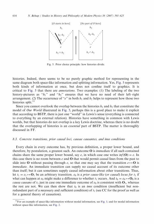
The idea of history is essential to the definition of ‘‘space-like related’’: e1 SLR e2 ifneither e1pe2 nor e2pe1, but nevertheless e1 and e2 are consistent (there is a history, h, towhich both belong). Histories branch in their own way, as governed by the followingaxiom, called the prior choice principle:
Let an outcome chain O be a subset of history h1 and excluded
from history h2; then there is a point event e that is in the past
of O and maximal in h1 \ h2: See Fig. 5. ð21Þ
The point e is called a choice point: e and all point events in its causal past belong to bothh1 and h2, whereas every pair of point events fe1; e2g with eoe1 2 h1 and eoe2 2 h2 isinconsistent. Fig. 5 illustrates a simple case. Time-like goes up and down, space-like goesleft and right, and the dotted lines are tracks of the light-speed limitation on velocities.Obviously when left–right represents space-like separation, you cannot in the same figurelet it represent alternative histories, and vice versa. In Fig. 5, the picture of each historyalready uses left–right to indicate space-like separation. For this reason, you should not,on pain of confusion, use left–right also to indicate the modal idea of the splitting of
ARTICLE IN PRESS
e
h2
h1−h2h2−h1
e
h1
O
[No part of O here][O starts in here]
h1 ∩ h2 h1 ∩ h2
Fig. 5. Prior choice principle: how histories divide.
N. Belnap / Studies in History and Philosophy of Modern Physics 38 (2007) 593–625614
histories. Indeed, there seems to be no purely graphic method for representing in thesame diagram both space-like information and splitting information. Yes, Fig. 5 representsboth kinds of information at once, but does not confine itself to graphics. It iscritical to Fig. 5 that there are annotations. Two examples: (1) The labeling of the twohistory-pictures as ‘‘h1’’ and ‘‘h2’’ ensures that we have no need of their left–rightarrangement. (2) The occurrence of ‘‘e’’ in both h1 and h2 helps to represent how those twohistories split.11
Since you cannot overlook the overlap between the histories h1 and h2 that constitute themodel of Our World illustrated in Fig. 5, perhaps this is a good place to make it explicitthat according to BSTP, there is just one ‘‘world’’ in Lewis’s sense (everything is connectedto everything by an external relation). Histories have something in common with Lewisworlds, but that histories do not overlap is a key Lewis doctrine, whereas there is no doubtthat the overlapping of histories is an essential part of BSTP. The matter is thoroughlydiscussed in FF.
8.3. Concrete transitions, prior causal loci, causae causantes, and inus conditions
Every chain in every outcome has, by previous definition, a proper lower bound, andtherefore, by postulation, a greatest such. An outcome O is immediate if all such containedchains share the same proper lower bound, say e, in which case one writes inf ðOÞ ¼ e. Inthis case there is no room between e and O that would permit causal lines from the past toslide into O without passing through e, so that one may say that the transition e:O isimmediate. An immediate transition can supply no causal account of its outcome otherthan itself; but it can sometimes supply causal information about other transitions. Thus,let t1 ¼ e1:O1 be an arbitrary transition. e0 is a prior cause-like (or causal) locus for t1 ifwhat can happen at e0 might make a difference to whether t1 occurs. And t0 ¼ e0:O0 is acausa causans of t1 just in case one immediate outcome of e0 is consistent with O1, whereasthe rest are not. We can then show that t0 is an inns condition (insufficient but non-redundant part of a necessary and sufficient condition) of t1 (see CC for the proof as well asfor a general theory of causation).
11For an example of space-like information without modal information, see Fig. 1; and for modal information
without space-like information, see Fig. 2.

ARTICLE IN PRESSN. Belnap / Studies in History and Philosophy of Modern Physics 38 (2007) 593–625 615
8.4. Probabilities in branching space-time: the WBM analysis
Weiner & Belnap (2006) and Muller (2005), in spite of being independent and offeringdistinct results and perspectives, benefited to a certain extent from pre-publicationconversations; it is proper to think of their work in terms of mutual assistance. Onefundamental idea of the ‘‘WBM’’ construction is that you look to the set ccðI:OÞ ofcausae causantes (certain basic transitions; see CC) as containing all and only theinformation needed for assigning a propensity to I:O (p. 491). There are now two(equivalent) ways to proceed. Each basic transition e:H among those causae causantes
has its own local causal alternatives e:H1 based on keeping its initial e and letting itsbasic outcome H1 vary over all the basic outcomes of e. Muller develops more ‘‘global’’causal transitions by piecing together those basic-transition causal alternatives to themaximum extent that they can consistently be fit together. These maximal consistent sets ofbasic causal alternatives are the sample space, A, underlying one way of calculating thepropensity belonging to I:O. By taking the family of all subsets of the sample space, youinevitably get the boolean algebra, F, that must underlay the causal-probability field of setsin the context of which giving a propensity to I:O makes inescapable sense (recall thatwe are thinking finite). From this point of view, one has only to add a standardKolmogorov measure, m, defined on the algebra, F, and yielding values in the interval½0; 1�. Since the unit set fccðI:OÞg is bound to be an element of the algebra, F, that isenough. One may now define the causal-probability space appropriate to I:O as hA;F ;mi.
A second way to proceed, exploited in Weiner & Belnap (2006), derives the wantedpropensities prðI:OÞ from a distributed measure m ¼ fneje is a prior causal locus of I:O
and ne is a probability measure on the boolean algebra, pe, of all immediate outcomes of e,and thus a measure (the very ‘‘same’’ measure) defined on each of the basic transitionse:O. Define a propensity space for I:O as a pair hT ; ni, where T is the set of all causae
causantes of I:O together with, for each prior causal locus e, the set of all basictransitions e:H; and where n maps each member of T into the interval ð0; 1Þ, subjectonly to the restriction that for each prior causal locus, e, that figures in T,
X
h2HðeÞ
nðe:pehhiÞ ¼ 1.
That is, from the perspective of e, something must happen.The second way, which begins with a separate, local, and independent measure for each
set e:pe, has the virtue of firm and direct rooting in the idea of propensity. It quicklyleads to correct intuitive judgments in easy cases, cases in which we obtain the propensityof I:O by multiplying together all the propensities of all its causae causantes.
On the other hand, the relation of the second way to global Kolmogorov probabilities isless obvious; it is surely not made clear in Weiner & Belnap (2006). The second waynevertheless turns out to be conceptually equivalent to the first way, as one would hoperegarding a pair of ways one of which is top-down and the other bottom-up.
9. Application to corkscrew story
Salmon told (at least) two ‘‘inversion stories,’’ one, the can opener story, in Salmon(1984), and one, the corkscrew story, in Salmon (1989). With these stories he subscribed to

ARTICLE IN PRESSN. Belnap / Studies in History and Philosophy of Modern Physics 38 (2007) 593–625616
the position that propensities ‘‘make sense as direct probabilities . . . ; but not as inverseprobabilities (because the causal direction is wrong)’’ (p. 88). Salmon furthermoreexpressed the view that ‘‘probabilistic causality is fraught with difficulties’’ that such asReichenbach (1956), and Suppes (1970) do not overcome. I agree with both verdicts, whilestill endorsing the BSTP theory of causal probability as a sensible account of some of thedeepest properties of causal probabilities. BSTP is sufficiently different from any worked-out theory in the literature that it needs to be evaluated by itself, untainted by associationwith other theories.My plan is to retell the corkscrew story with the help of BSTP, leaving the reader to
judge whether BSTP helps. Here is how Salmon (1989) put the matter.
Imagine a factory that produces corkscrews. It has two machines, one old and onenew, each of which makes a certain number per day. The output of each machinecontains a certain percentage of defective corkscrews. Without undue strain, we canspeak of the relative propensities of the two machines to produce corkscrews (eachproduces a certain proportion of the entire output of the factory), and of theirpropensities to produce defective corkscrews. If numerical values are given, we cancalculate the propensity of this factory to produce defective corkscrews. So far, sogood. Now, suppose an inspector picks one corkscrew from the day’s output andfinds it to be defective. Using Bayes’s theorem we can calculate the probability thatthe defective corkscrew was produced by the new machine, but it would hardly bereasonable to speak of the propensity of that corkscrew to have been produced by thenew machine (p. 88).
In retelling the story, I shall rely on an annotated BSTP diagram, namely Fig. 6, whichyou should put before you. Each hj (j ¼ 1; . . . ; 5) in that figure is a history. e0 is areference point event before all the action. The ellipses are machines Mi ði ¼ 1; 2Þ,with ei the (idealized) point event of production by Mi. e3 is the choice point for theInspector (when he has a choice). Di ½Gi� is a defective [good] corkscrew producedby machine Mi. fdi; gi ði ¼ 1; 2Þg represent the two possible immediate outcomes ofeach machine choice point e1; e2, whereas d�i ði ¼ 1; 2Þ represent the two possiblepickings by the Inspector from Box-b at e3. If two areas have the same label, they areidentical; otherwise, not. The boxes a and b are only receptacles. In the story that Fig. 6illustrates, machines M1 and M2 (the gray ellipses) make different numbers of corkscrewsper day, and also have different propensitiesfor making, on each run, a defectivecorkscrew.To illustrate a BSTP story about many physical objects requires drawing many tracks
through the space-time of each history, which is a pain. For this reason, with theexpectation that it will not make any difference, and because this is in part a test of makingsense of single-case propensities, I am going to have each machine make just one corkscrewper day. (This expository strategy also reduces the temptation to measure propensities interms of frequencies.) The propensity of each machine to turn out a defective corkscrew ona given day is given numerically in the interval ½0; 1�; say M1 has a .4 propensity of makinga defective corkscrew, and consequently a .6 propensity for making a good one. Let thepropensities for M2 be .1 defective and .9 good. In BSTP these propensities qualify,respectively, four of the relevant basic transitions (each expressed in two ways) having one

ARTICLE IN PRESS
D1
D1
D2 D1
D2
D2
Box β
Box α
Box β
Box α
G1 G2
Box β
Box αG1
D2
D2 D1
D1
G2
d1
d*1
d1
d1g1 g1
d2
d*2
d2 g2 g2
d2
Box β
Box α
Box β
Box α
h1
h5h4h3
h2
e2e1e2e1e2e1
e2e1e2e1
0.1 0.6 0.9 0.4 0.9
0.10.60.6 0.1
0.7 0.3
0.4
M1 M2 M1 M2 M1 M2
M2M1M2M1
e3e3
e0 e0 e0
e0e0
4:02
4:01
4:00
4:02
4:01
4:01
4:00
4:00
4:01
4:00
Fig. 6. The corkscrew story.
N. Belnap / Studies in History and Philosophy of Modern Physics 38 (2007) 593–625 617
of e1 or e2 as initial:
prðe1:pe1hg1iÞ ¼ :4 ¼ prðe1:fh3; h5gÞ,
prðe1:pe1hd1iÞ ¼ :6 ¼ prðe1:fh1; h2; h4gÞ,
prðe2:pe2hg2iÞ ¼ :9 ¼ prðe2:fh4; h5gÞ,
prðe2:pe2hd2iÞ ¼ :1 ¼ prðe2:fh1; h2; h3gÞ. ð22Þ
It is part of Salmon’s story that one day
the Inspector picks one corkscrew from the day’s output and finds it defective(Salmon, 1989).
Salmon’s Humphreys-inspired Bayes-type question then arises: What shall we say aboutthe corkscrew’s propensity to have been made by M1? His answer: ‘‘it would hardly bereasonable to speak of the propensity of that corkscrew to have been produced by’’ M1. Itcertainly does sound like double talk. The Inspector examines a corkscrew, only to find itdefective. Does anyone want to say that the corkscrew lying quietly in his hand has acertain propensity to—what? Propensity to have been made by machine M1 rather thanM2? But that seems nonsense. Calculate a subjective probability if you wish; there isnothing wrong with ‘‘Given what I know, it is reasonable to believe that there is a good

ARTICLE IN PRESSN. Belnap / Studies in History and Philosophy of Modern Physics 38 (2007) 593–625618
chance that the corkscrew was made by machine M1,’’ so that you can likely finda guide for your inferring, should you wish to so engage yourself. Or work out whateverobjective correlations you like, survive the Problem of the Reference Group, and put yourmoney down. Correlations may be objective, but they have no ‘‘direction,’’ whereaspropensities are all about influencing the future. The corkscrew was in fact made in thesettled past either by machine M1 or machine M2, and current chancy propensity is non-existent.We nevertheless need to go further into the ‘‘deep structure’’ of the story in two ways.
First, Salmon uses language that attributes propensities to objects: ‘‘we can speak of therelative propensities of the two machines . . . to produce defective corkscrews.’’ (The samelanguage is used in the can opener story of Salmon, 1984, p. 205.) But in attributingpropensities to objects, we threaten to abandon the ‘‘single case.’’ Basic single-case
propensities are more nearly tied to transition events, not to objects, and not only because ofwanting to adhere to the single case. In addition, the English passive can be used to illeffect: Salmon’s active-voice ‘‘The propensity of each machine to turn out a defectivecorkscrew on a given day’’ could be turned into ‘‘the propensity for a defective corkscrewto be turned out by each machine,’’ is, though equivalent by the standard passivetransformation, less clear as to the bearer of the propensity. It is, however, perfectlyrational to relate propensities for objects to transition propensities by way of complexevents, for example by attributing a propensity to a whole series (or cloud or continuum)of transitions rooted in point events in a space-time-like event-locale. BSTP has theresources for this generalization (see Muller, 2005). Just do not make it without noticingwhat you are doing, or without careful conceptualization. If, when theorizing, weconsistently attribute propensities to transition events, we shall be less likely to fall into thesoup.Second, the rhetoric suggests that all the indeterminism is fastened on the respective
occasions e1 and e2 of production of the corkscrews, respectively, by M1 and M2. Not so:Salmon is explicit that the Inspector picks one corkscrew from the day’s output. He is evenmore explicit in telling the can opener story: ‘‘Someone randomly picks a can opener out ofthe box’’ (Salmon, 1984, p. 205). That makes the Inspector’s random pick of a corkscrew(or can opener) a causa causans, and one not to be ignored in drawing philosophicalpictures or morals.Fig. 6 features Box a and Box b as part of my retelling of the corkscrew story. Boxes, like
corkscrews and inspectors, are substances that can be re-identified even when coincidentwith radically distinct point events in BSTP. (Were I to be distracted by problemssurrounding this pronouncement, I would take my argle-bargle from Wiggins (2001),extending the arguments from linear time to branching space-time. In the meantime, I begyou not to suggest that Fig. 6 shows 10 boxes!) For the corkscrew story we need two boxes,Box a and Box b. The minute the corkscrews come out of the two machines, they aremechanically dumped into Box a. (All the dotted lines in Fig. 6 represent paths in a singlehistory; motion along them is deterministic.) From the perspective of the point event, e0, inthe causal past of the whole of a day’s running of the machines, Box a can be filled in oneof four ways: (1) A good corkscrew from M1 and a defective corkscrew from M2, which welabel, respectively, G1 (‘‘G’’ for ‘‘good’’) and D2 (‘‘D’’ for ‘‘defective’’); (2) the reversecombination labeled D1 and G2; (3) two good corkscrews, labeled G1 and G2; or, finally, (4)two defective corkscrews labeled D1 and D2. We have up to this point emphasized only thefour transitions (22) that stretch forward from the initials e1 and e2.

ARTICLE IN PRESSN. Belnap / Studies in History and Philosophy of Modern Physics 38 (2007) 593–625 619
9.1. The Inspector
Then along comes the Inspector. He or she ignores any good output in Box a, payingattention only to defective corkscrews. In a case in which Box a has a single defectivecorkscrew, as happens in histories h3 and h4, the Inspector is offered only a Hobson’sChoice, and that uniquely defective corkscrew is deterministically moved to Box b. In thecase in which Box a contains no defectives, as in h5, the Inspector deterministically leavesall as it is, making no transfer to Box b. Naturally in this case the Inspector cannot succeedin gathering up a defective corkscrew. There remains the case in which two defectivecorkscrews were put into Box a, as illustrated in histories h1 and h2. Since the Inspector isto pick, in this case the story tells us that the Inspector indeterministically chose whichdefective corkscrew to transfer to Box b. (Otherwise we might say that the inspection wasfixed.)
You can tell from Salmon’s calculations that the Inspector’s choice was Laplacian, withan equal chance for each corkscrew in Box a. That is, however, a thesis of no bearing onthe point of the story, so with good reason Salmon simply does not say what the chancesare for this propensive picking of a defective corkscrew from Box a. Let us (you and I) saythat in the case when there are two defective corkscrews in Box a, the Inspector has apropensity of .3 for M1’s defective output and (of course) a .7 propensity for picking thedefective output of M2. Perhaps we should not; perhaps we should just assume that thechances are 50/50, in order to stay closer to the presumed intent of Salmon’s story. But letus go with 30/70 just to have calculations that seem easier to keep straight. The choicepoint for the Inspector’s pick, that is, e3, must come after all the defective corkscrews arealready in Box a (or else you have a different story). The propensity distribution for all ofthe causae causantes based on each of the choice points e1; e2, and e3, can now be describedas follows:
prðe1:pe1hg1iÞ ¼ :4 ¼ prðe1:fh3; h5gÞ ¼ :04þ :36,
prðe1:pe1hd1iÞ ¼ :6 ¼ prðe1:fh1; h2; h4gÞ ¼ :042þ :018þ :54,
prðe2:pe2hg2iÞ ¼ :9 ¼ prðe2:fh4; h5gÞ ¼ :54þ :36,
prðe2:pe2hd2iÞ ¼ :1 ¼ prðe2:fh1; h2; h3gÞ ¼ :042þ :018þ :04, ð23Þ
prðe3:pe3hd�1iÞ ¼ :7 ¼ prðe3:fh1gÞ ¼ :7,
prðe3:pe3hd�2iÞ ¼ :3 ¼ prðe3:fh2gÞ ¼ :3.
From this table, because it includes all the relevant causae causantes, we can construct atable of the non-basic propensities, in particular the table of propensities of the varioustransitions e0:pe0hhii for 1pip5:
prðe0:pe0hh1iÞ ¼ :042 ¼ :6� :1� :7,
prðe0:pe0hh2iÞ ¼ :018 ¼ :6� :1� :3,
prðe0:pe0hh3iÞ ¼ :04 ¼ :4� :1,
prðe0:pe0hh4iÞ ¼ :54 ¼ :6� :9,
prðe0:pe0hh5iÞ ¼ :36 ¼ :4� :9. ð24Þ
You can also start with this table, (24), whose entries show propensities from a suitablyearly initial to a maximally precise outcome, and finish with the previous table, (23).

ARTICLE IN PRESSN. Belnap / Studies in History and Philosophy of Modern Physics 38 (2007) 593–625620
9.2. Inversion
Having the advantage of a thorough working-out of the story, let us go back now andsay what needs to be said about the inversion in question. First, the attribution of aforward propensity with ‘‘the propensity of each machine to make a defective corkscrew.’’By Fig. 6 we are asking for the propensity of the basic transition from the production-pointei of each machine Mi to the immediate outcome di that guarantees a defective corkscrewfrom that machine; namely, prðe1:pe1hd1iÞ ¼ prðe1:fh1; h2; h4gÞ, which by (23) is .6; andalso the propensity of prðe2:pe2hd2iÞ ¼ prðe2:fh1; h2; h3gÞ, which, is .1. So ‘‘.6’’ and ‘‘.1’’are the straightforward answers to ‘‘For each machine, what propensity does it have (at4:00) to make a defective corkscrew?’’It should be clear that the probability of a transition is not the same as a standard
conditional probability, whether defined in terms of absolute probabilities or not. In fact,I wonder if there is anything conditional here whatsoever. In an earlier publicationI suggested that a transition such as prðe1:pe1hd1iÞ is an ‘‘event-conditional,’’ a suggestionthat arose from the observation that the ‘‘antecedent’’ must be an event rather than aproposition, since it must supply a locus in Our World. (Thinking of events as sets of point-events and of propositions as sets of histories, the former do have such a locus, whereaspropositions do not. This point arises repeatedly in the BST papers.) It was nevertheless,I now think, not a profitable suggestion. What is wrong is the ‘‘conditional’’ part: Theantecedent simply does not supply any kind of condition. I then suggested that, inasmuch aswe are looking at a transition from e1 to d1, the antecedent event supplies a ‘‘perspective.’’ Onemight try reading prðe1:pe1hd1iÞ ¼ :4 as ‘‘from the perspective of e1, the propensity for d1
coming to pass is .4.’’ I think that may help some, but it rubs somewhat against the grain ofBSTP: To suggest that the ‘‘action’’ lies with the outcome, d1, with e1 as only a passiveonlooker, certainly seems to underplay the relational aspect of a transition. Attributing apropensity-strength to a transition I:O is, in this respect as well, a major difference fromattributing a conditional probability, for the reading ‘‘Given B, the probability of A ¼ p,’’which rhetorically fastens the probability onto A, is eminently satisfactory. The reading movesB into the background, where it belongs, so that the role of A can be emphasized. These are ofcourse rhetorical points, but I do think that they deserve consideration.It is perhaps helpful to pursue the analogy between a BSTP transition e:O that represents
a propensity and a position vector as represented by an arrow. (1) The outcome, O, gives a‘‘direction’’ to the propensity in analogy to the direction of the arrow, (2) the initial e providesa ‘‘starting position’’ in Our World in analogy to the position of the tail of the arrow, and (3)the strength p of the propensity is analogous to the length of the arrow. That analogy urgesthat propensities are essentially relational. It is of course all right, even necessary, in English tospeak of the propensity as being ‘‘of’’ the initial and ‘‘for’’ the outcome, but for accuracy it allhas to be said in one rush of air. In the following lists, note how the degree of the propensitieschange as one varies either the initial (what follows the ‘‘of’’ in ‘‘the propensity of . . .’’) or theoutcome (what follows the ‘‘for,’’ or some other preposition, in ‘‘propensity for . . .’’).
This batch varies the initial while keeping the outcome constant:
prðe1:pe1hd�1iÞ ¼ :042,
prðe2:pe2hd�1iÞ ¼ :07,
prðe3:pe3hd�1iÞ ¼ :7. ð25Þ
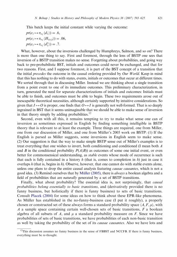
ARTICLE IN PRESSN. Belnap / Studies in History and Philosophy of Modern Physics 38 (2007) 593–625 621
This batch keeps the initial constant while varying the outcome:
prðe1:pe1hd1iÞ ¼ :6,
prðe1:pe1hH ðe3ÞiÞ ¼ :06,
prðe1:pe1hd�1iÞ ¼ :7.
What, however, about the inversions challenged by Humphreys, Salmon, and so on? Thereis more than one thing to say. First and foremost, through the lens of BSTP one sees thatinversion of a BSTP transition makes no sense. Forgetting about probabilities, and going wayback to pre-probabilistic BST, initials and outcomes could never be exchanged, and that fortwo reasons. First, and I suppose foremost, it is part of the BST concept of a transition thatthe initial precedes the outcome in the causal ordering provided by Our World. Keep in mindthat this has nothing to do with states, events, initials or outcomes that occur at different times.We sorted through that in discussing Miller. Instead we are thinking about a single transitionfrom a point event to one of its immediate outcomes. This preliminary characterization, inturn, generated the need for separate characterizations of initials and outcomes: Initials mustbe able to finish, and outcomes must be able to begin. These two requirements arose out ofinescapable theoretical necessities, although certainly supported by intuitive considerations. Sogiven that I:O is proper, one finds that O:I is generally not well-formed. That is so deeplyingrained in BST that it seems unimaginable that we should be able to make sense of inversionin that theory simply by adding probabilities.12
Second, even with all this, it remains tempting to try to make what sense one can ofinversion as sometimes expressed in English by finding something intelligible in BSTPtheory that is relevant to at least the example. Three things are required, one from Miller,one from our discussion of Miller, and one from Muller’s 2005 work on BSTP: (1) If theEnglish is parsed as Miller suggests, some inversions in English seem to make sense.(2) Our suggestion is that the way to make simple BSTP sense out of Miller’s examples is totreat everything that one wishes to invert, both conditioning and conditioned (I mean both A
and B in the conditional probability PðAjBÞ) as outcomes of some one initial event, or evenbetter for commonsensical understanding, as stable events whose mode of occurrence is suchthat each is fully contained in a history h (that is, comes to completion in h) just in case itoverlaps h (that is, begins in h). Observe, however, that one cannot do with stable events alone,unless one plans to drop the entire causal analysis featuring causae causantes, which is not agood idea. (3) Remind ourselves that by Muller (2005), there is always a boolean algebra and afield of probabilities that are naturally generated by a set of BSTP transitions.
Finally, what about probability? The essential idea is, not surprisingly, that causal
probabilities belong essentially to basic transitions, and (derivatively provided there is nofunny business, but holistically if there is funny business) to sets of basic transitions.Consult Placek (2004) for some ideas on how to think about these EPR-like phenomena.As Muller has established in the no-funny-business case (I put it roughly), a properlychosen or constructed set of these always forms a standard probability space hA;F ;mi, withA a sample space containing certain well-chosen sets of basic transitions, F a booleanalgebra of all subsets of A, and m a standard probability measure on F. Since we haveprobabilities of sets of basic transitions, we have probabilities of each non-basic transitionas well by taking the probability of the set of its causae causantes. Also we have lots and
12This discussion assumes no funny business in the sense of FBBST and NCCFB. If there is funny business,
everything must be re-thought.

ARTICLE IN PRESSN. Belnap / Studies in History and Philosophy of Modern Physics 38 (2007) 593–625622
lots of standard conditional probabilities, which will in fact have a causal meaning of sortssince they are based on probabilities of basic transitions; that is, since they are based onpropensities.For a single example of a standard conditional probability that parrots Salmon’s query,
From the perspective of e0, what is the probability that the Inspector takes acorkscrew made by machine M1, given that he takes a defective corkscrew?
My calculation is disappointingly simple because of the extreme simplicity of my version ofthe corkscrew example, but since it is only principle that is at stake, I will persevere. Thecalculation is this:
The Inspector takes a corkscrew produced by M1 in histories h1 and h4. TheInspector takes a defective corkscrew in histories h1, h2, h3, and h4. (Just look at whatis in box b. Note: ‘‘Take’’ is not intended to imply ‘‘picked’’ or ‘‘chose,’’ so theHobson’s choices count.)
prðe0:fh1; h2; h3; h4gÞ ¼ :64,
prðe0:fh1; h4gÞ ¼ :582,
Pe0ðfh1; h4gjfh1; h2; h3; h4gÞ ¼:582
:64,
Pe0ðfh1; h2; h3; h4gjfh1; h4gÞ ¼ 1. ð26Þ
The subscript e0, which here represents a perspective, is intended to fill out an echo of thethree-termed relation of Miller and of Humphreys that we earlier canvassed. The last line isthe conditional probability of the Inspector taking a defective corkscrew given that hetakes a product of M1. The answer in this case is an uninteresting ‘‘1’’ because the set-upimplies that the Inspector takes only defective corkscrews.So that illustrates how, starting with causal probabilities and propensities attached only
to causae causantes, one can have a rich feast of standard probabilities with standardconditional probabilities and all that jazz. Which of course is far from saying thatpropensities are standard probabilities, or that standard probabilities are propensities. Theupshot is rather that BSTP lets one investigate both, together with their interconnections,without sacrificing either.
10. Closing remarks
So what should we conclude? Is BSTP causal probability theory right for objectivepropensities or not? It seems best to close with some short answers.
1.
A partial answer to our covering question is that propensities have a causal aspect,which Kolmogorov probability theory does not see or need to see. Objective probability,by itself, has nothing to say about causation. The work of Humphreys, Miller, etc., showthat much to a fare-thee-well, although they refrain from drawing the strong conclusion.Nor is this conclusion impugned by decades of work issuing in suggestions of how to getsomething objectively causal out of objective probabilities, for in every case of whichI know, the ‘‘how to’’ involves (sometimes implicitly, sometimes explicitly) somethingdoxastic or epistemic.
ARTICLE IN PRESSN. Belnap / Studies in History and Philosophy of Modern Physics 38 (2007) 593–625 623
2.
BSTP theory provides a useful background for sorting out some of the argumentsconcerning the relations between probability and propensity; BSTP helps us see that thenew language shared by Humphreys and Miller, while intuitively all right, is in need of afull working out that will meet the standards of Frege. To that extent, you cannot fullytrust any conclusions of the debate that are stated in those terms.3.
Are propensities correctly described by probability theory? Humphreys took one side,coming to a negative conclusion, which I share: You cannot get a propensity outof a probability. It was surprising to find out, as it were, that the essence of theHumphreys (1985) argument—at least according to the BSTP analysis—did not involveprobabilities; the argument was entirely causal, in the sense that BST borrows fromspecial relativity.4.
Miller took the other side, coming to the positive conclusion that the bug-a-boo ofBayesian inversion can be dismissed as a non-problem. BSTP agrees with Miller thattime-reversal is not a problem: I relied on ideas from BSTP to argue that as long as oneis dealing only with BSTP outcomes, time-reversal (or Bayesian reversal of ðAjBÞ) is fine.So there is a place for Bayes reversal in propensity theory, as long as outcomes ride onboth sides of the vertical. On the other hand, BSTP says that you cannot reverse initialand outcome of a transition. They must sit in the causal order. Exactly what this meansand why it is true is part of the theory of causae causantes, Belnap (2005b).5.
Sometimes it is tempting to try to get causality or ‘‘the direction of time’’ out ofprobability theory in the sense of the Kolmogorov axioms, but this entire enterprisemay be misguided. One cannot know unless the part of the theory involving causal andspatio-temporal concepts is laid out with a rigor equal to that of the probability part.Certainly the classic examples, and there are many such, do not live up to this ideal. Myknowledge of this research area is not deep, so I do not plead for a grant of authority.I am thinking of pioneers such as Simon (1957), Lazarsfeld (1958), Suppes (1970), andmore recently Glymour, Spirtes, & Scheines (2001), all of whom are strictly rigorouswith respect to probability theory, but not comparably rigorous with respect to space-time and the like. It seems to me just another case of ‘‘you only get out what you putin.’’6.
BSTP does not encourage treating prðI:OÞ as a conditional probability that shouldever be defined byprðI \OÞCprðOÞ.
What stands in the way is not only that an initial I when intersected with one of itsoutcomes O typically yields ;, the empty set. In addition, the idea of an ‘‘absolutepropensity’’ such as might be nominated by prðIÞ or prðOÞ seems to be unintelligible.Indeed, BSTP always distinguishes conditional probabilities PðAjBÞ from propensitiesprðI:OÞ. PðAjBÞ is dealing with proportions, prðI:OÞ with causal structure. It ishardly a new thought that inferring objective causal structure from statistics is nomatter of definition.
7.
How should we then interpret the propensity prðI:OÞ? Let us go wholesale along withMuller (2005). The interpretation is definitely and explicitly and rigorously going to be aprobability—though not merely a probability: It wears its causal structure on its face.You first find the set ccðI:OÞ of basic transitions that stand as causae causantesof I:O. An arbitrary (finite) set of basic transitions gives rise via BST structure
to an eminently satisfying notion of ‘‘maximal consistent subset of ccðI:OÞ.’’

ARTICLE IN PRESSN. Belnap / Studies in History and Philosophy of Modern Physics 38 (2007) 593–625624
The terminology guides us to see how natural it is to form the boolean algebra, B, withthose maximal consistent subsets, A, as atoms. From there one needs to reach out but ahand’s breadth in order to identify a suitable representative of I:O as a particular set,S, in the algebra B. Backing up just a little, one can see how the atoms serve as ‘‘middleterms’’: a propensity for each basic transition yields, by multiplication, a ‘‘propensiveprobability’’ for each atom, and hence, by addition, a propensive probability, p, for theset of atoms, S. Finally, the special relationship between S and I:Omakes sense out oftransferring p from S to I:O: prðI:OÞ ¼ p. I think that this analysis and theorem ofMuller (2005), though tucked away here in penultimate position, is the most powerfulresult that anyone has obtained in BSTP theory.
8.
I add two remarks. (1) It seems to me that BSTP helps out propensities very much morethan vice versa, chiefly because BSTP is an exact theory and propensity-theory is not.Indeed, there would be little in the BSTP portions of this essay that would needrewording (for sense) if ‘‘propensity’’ was dropped in favor of some jaw-breaker like‘‘objective single-case causal transition probability as idealized in BSTP.’’ (2) BSTPtheory attaches propensities to basic transitions (and to transitions more generally), butit is difficult or impossible to stay faithful to that attachment in informal English. I havenot tried very hard, since, although I am far from sure, I do not think that there is muchbenefit at this stage of getting straight on all the variations in the syntax of the noun‘‘propensity.’’ Maybe next year. At this stage, the theory does not do well at teachingone how to talk. It is, however, pretty good at saying how one should think aboutpropensities, as I take it is illustrated by the rigorous treatment in Section 4 ofHumphrey’s Paradox, and in Section 9 of Salmon’s corkscrew story.References
Belnap, N. (1992). Branching space-time. Synthese, 92, 385–434 See Belnap, N. (2003a).
Belnap, N. (1999). Concrete transitions. In: G. Meggle (Ed.), Actions, norms, values: Discussions with Georg
Henrik von Wright (pp. 227–236). Walter de Gruyter, Berlin. A ‘‘postprint’’ (2002) may be obtained from
hhttp://philsci-archive.pitt.edui.
Belnap, N. (2002a). Double time references: Speech-act reports as modalities in an indeterminist setting. In
F. Wolter, H. Wansing, M. de Rijke, & M. Zakharyaschev (Eds.), Advances in modal logic, Vol. 3 (pp. 37–58).
Singapore: World Scientific. A preprint of this essay may be obtained from hhttp://www.pitt.edu/�belnapi.
Belnap, N. (2002b). EPR-like ‘funny business’ in the theory of branching space-times. In T. Placek, &
J. Butterfield (Eds.), Non-locality and modality (pp. 293–315). Dordrecht: Kluwer Academic Publishers A
preprint of this essay may be obtained from hhttp://philsci-archive.pitt.edui.
Belnap, N. (2003a). Branching space-time, postprint, January, 2003. This is a postprint of Belnap (1992) that
includes a number of additional explanations and a little re-structuring. It may be obtained from hhttp://
philsci-archive.pitt.edui.
Belnap, N. (2003b). No-common-cause EPR-like funny business in branching space-times. Philosophical Studies,
114, 199–221 A non-quotable preprint may be obtained from hhttp://philsci-archive.pitt.edui.
Belnap, N. (2005a). Agents and agency in branching space-times. In D. Vanderveken (Ed.), Logic, thought and
action (pp. 291–313). Dordrecht: Springer.
Belnap, N. (2005b). A theory of causation: Causae causantes (originating causes) as inus conditions in branching
space-times. British Journal for the Philosophy of Science, 56, 221–253 A preprint of this essay may be obtained
from hhttp://philsci-archive.pitt.edui.
Belnap, N., Perloff, M., & Xu, M. (2001). Facing the future: Agents and choices in our indeterminist world. Oxford:
Oxford University Press.
Gillies, D. (2000). Varieties of propensity. British Journal for the Philosophy of Science, 51, 807–835.
Glymour, C., Spirtes, P., & Scheines, R. (2001). Causation, prediction and search (2nd revised ed.). Cambridge:
MIT Press First edition, 1993, by C. Glymour, Springer.

ARTICLE IN PRESSN. Belnap / Studies in History and Philosophy of Modern Physics 38 (2007) 593–625 625
Humphreys, P. (1985). Why propensities cannot be probabilities. The Philosophical Review, 94, 557–570.
Humphreys, P. (2004). Some thoughts on Wesley Salmon’s contributions to the philosophy of probability.
Philosophy of Science, 71, 942–949.
Lazarsfeld, P. F. (1958). Evidence and Inference in Social Research. Daedalus, 87, 99–130.
Miller, D. (1994). Critical rationalism. A restatement and defense. Chicago and La Salle: Open Court Publishing
Company.
Miller, D. (2002). Propensities may satisfy Bayes’s theorem. In R. Swinburne (Ed.), Bayes’s theorem, Proceedings
of the British Academy, Vol. 113 (pp. 111–116). Oxford: Oxford University Press.
Muller, T. (2002). Branching space-time, modal logic and the counterfactual conditional. In T. Placek, &
J. Butterfield (Eds.), Non-locality and modality (pp. 273–291). Dordrecht: Kluwer Academic Publishers.
Muller, T. (2005). Probability theory and causation: A branching space-times analysis. British Journal for the
Philosophy of Science, 56, 487–520.
Placek, T. (2000a). Is nature deterministic? Krakow: Jagiellonian University Press.
Placek, T. (2000b). Stochastic outcomes in branching space-time: Analysis of Bell’s theorem. British Journal for
the Philosophy of Science, 51, 445–475.
Placek, T. (2004). Quantum state holism: A case for holistic causation. Jagiellonian University.
Popper, K. (1959). The propensity interpretation of probability. The British Journal for the Philosophy of Science,
10, 25–42.
Prior, A. (1957). Time and modality. Oxford: Oxford University Press.
Reichenbach, H. (1956). The direction of time. Berkeley: University of California Press.
Salmon, W. C. (1984). Scientific explanation and the causal structure of the world. Princeton: Princeton University
Press.
Salmon, W. C. (1989). Four decades of scientific explanation. Minneapolis: University of Minnesota Press.
Simon, H. A. (1957). Models of man: Social and rational. New York: Wiley.
Suppes, P. (1970). A probabilistic theory of causality, Acta philosophica fennica, Vol. 24. Amsterdam: North-
Holland.
Thomason, R. H. (1970). Indeterminist time and truth-value gaps. Theoria, 36, 264–281.
Thomason, R. H. (1984). Combinations of tense and modality. In D. Gabbay, & G. Guenthner (Eds.), Handbook
of philosophical logic, Vol II: Extensions of classical logic, Synthese Library, Studies in epistemology, Vol. 165
(pp. 135–165). Dordrecht: Reidel.
Thomson, J. J. (1977). Acts and other events. Ithaca: Cornell University Press.
von Wright, G. H. (1963). Norm and action. A logical inquiry. London: Routledge & Kegan Paul.
Weiner, M., & Belnap, N. (2006). How causal probabilities might fit into our objectively indeterministic world.
Synthese, 149, 1–36.
Wiggins, D. (2001). Sameness and substance renewed. Cambridge: Cambridge University Press.