propagation of intense uv filaments and vortices
TRANSCRIPT

University of New MexicoUNM Digital Repository
Mathematics & Statistics ETDs Electronic Theses and Dissertations
2-1-2012
Propagation of intense UV filaments and vortices.Alexey Sukhinin
Follow this and additional works at: https://digitalrepository.unm.edu/math_etds
This Dissertation is brought to you for free and open access by the Electronic Theses and Dissertations at UNM Digital Repository. It has beenaccepted for inclusion in Mathematics & Statistics ETDs by an authorized administrator of UNM Digital Repository. For more information, pleasecontact [email protected].
Recommended CitationSukhinin, Alexey. "Propagation of intense UV filaments and vortices.." (2012). https://digitalrepository.unm.edu/math_etds/46

Candidate
Department This dissertation is approved, and it is acceptable in quality and form for publication: Approved by the Dissertation Committee: , Chairperson

Propagation of intenseUV filaments and vortices
by
Alexey Sukhinin
B.S., Taurida National University, Ukraine, 2002
M.S., Mathematics, University of New Mexico, USA, 2005
DISSERTATION
Submitted in Partial Fulfillment of the
Requirements for the Degree of
Doctor of Philosophy
Mathematics
The University of New Mexico
Albuquerque, New Mexico
December, 2011

c©2011, Alexey Sukhinin
iii

Dedication
To my parents Nickolay and Tatyana, for their support and help during all my life.
iv

Acknowledgments
First of all I would like to thank my adviser Alejandro Aceves for his help, advice,patience and support throughout the whole period of writing this dissertation. Imust acknowledge his professionalism and persistence as well as friendliness andability to make people feel good. I’m very grateful to Jean-Claude Diels and PavelLushnikov for their valuable comments. Special thanks to Stephen Lau for providingme with computational resources from Center for Advanced Research Computing aswell as many beneficial suggestions. I am very proud to have them in my dissertationcommittee. Also, I want to thank Sergey Dyachenko, Denis Silantyev and TaylorDupuy for fun and interesting conversations on different issues in theoretical physics.I’m indebted to Christina Hall for reading and checking my mistakes. Finally I wantto thank my parents, my sister and my nephew for understanding and support.
v

Propagation of intenseUV filaments and vortices
by
Alexey Sukhinin
ABSTRACT OF DISSERTATION
Submitted in Partial Fulfillment of the
Requirements for the Degree of
Doctor of Philosophy
Mathematics
The University of New Mexico
Albuquerque, New Mexico
December, 2011

Propagation of intenseUV filaments and vortices
by
Alexey Sukhinin
B.S., Taurida National University, Ukraine, 2002
M.S., Mathematics, University of New Mexico, USA, 2005
Ph.D., Mathematics, University of New Mexico, 2011
Abstract
The goal of this dissertation is to investigate the propagation of ultrashort high in-
tensity UV laser pulses of order of nanoseconds in atmosphere. It is believed that
they have a potential for stable and diffractionless propagation over the extended
distances. Consequently, it creates a new array of applications in areas of commu-
nication, sensing, energy transportation and others. The theoretical model derived
from Maxwell’s equations represents unidirectional envelope propagation and plasma
creation equations.
It was shown numerically through Newton’s iterations that the stationary model
permits the localized fundamental and vortex solutions. Discussion of the stability
of steady states involves different approaches and their limitations. Finally, model
equations are integrated numerically to study the dynamics of the beams in the
vii

stationary model as well as nanosecond pulses in the full (3+1)D model using parallel
computation.
viii

Contents
List of Figures xi
1 Introduction 1
2 The physical model 9
2.1 Derivation of propagation equation. . . . . . . . . . . . . . . . . . . . 9
3 Stationary solutions 17
3.1 The reduced model. . . . . . . . . . . . . . . . . . . . . . . . . . . . . 17
3.2 Nonlinear eigenvalue problem. . . . . . . . . . . . . . . . . . . . . . . 19
3.2.1 Plane wave solutions. . . . . . . . . . . . . . . . . . . . . . . . 20
3.2.2 Fundamental solutions. . . . . . . . . . . . . . . . . . . . . . . 21
3.2.3 Vortex solutions. . . . . . . . . . . . . . . . . . . . . . . . . . 25
4 Stability analysis 28
4.1 Semi-analytical approach. . . . . . . . . . . . . . . . . . . . . . . . . 29
ix

Contents
4.1.1 Gaussian Trial Function. . . . . . . . . . . . . . . . . . . . . . 29
4.1.2 Ring Trial Function. . . . . . . . . . . . . . . . . . . . . . . . 34
4.2 Stability of stationary solutions. . . . . . . . . . . . . . . . . . . . . . 36
4.2.1 Nonlinear stability. . . . . . . . . . . . . . . . . . . . . . . . . 37
4.2.2 Spatial perturbations. . . . . . . . . . . . . . . . . . . . . . . 38
4.2.3 Azimuthal perturbations. . . . . . . . . . . . . . . . . . . . . . 42
4.2.4 Spatiotemporal perturbations. . . . . . . . . . . . . . . . . . . 45
5 Numerical simulations 49
5.1 (2+1)D simulations. . . . . . . . . . . . . . . . . . . . . . . . . . . . 50
5.2 (3+1)D simulations. . . . . . . . . . . . . . . . . . . . . . . . . . . . 57
5.3 Numerical tests and convergence. . . . . . . . . . . . . . . . . . . . . 58
5.4 (3+1)D model with nonlinear losses. . . . . . . . . . . . . . . . . . . 63
6 Conclusion 68
Appendix A: Numerical method 70
References 73
x

List of Figures
1.1 Electrical discharge triggered by filamentation at atmospheric pres-
sure with focal positions (a) near mid-cell and (b) near the top elec-
trode of the cell [32]. . . . . . . . . . . . . . . . . . . . . . . . . . . 4
1.2 Experimental setup by Diels’ group . . . . . . . . . . . . . . . . . . 6
3.1 Plane wave solutions for m=1; (left)F (ψ2s) = F1(ψ2
s), (right)F (ψ2s) =
F2(ψ2s) . . . . . . . . . . . . . . . . . . . . . . . . . . . . . . . . . . 21
3.2 Comparison between numerically obtained steady state profile(solid)
at Λ = 0.205 and gaussian beam(dot-dashed) A20e−2r2/ω2
0 with power
400MW. . . . . . . . . . . . . . . . . . . . . . . . . . . . . . . . . . 25
3.3 Distribution of stationary vortex solutions for m = 1, 2, 3, 4 at Λ =
0.165 . . . . . . . . . . . . . . . . . . . . . . . . . . . . . . . . . . . 26
3.4 Comparison of numerical solution(solid) form=1 and approximation(dot-
dashed) A0re−r2/ω2
0 , A0 = 0.33, ω0 = 4 . . . . . . . . . . . . . . . . . 27
4.1 Propagation of the width of 380MW gaussian beam. . . . . . . . . . 31
4.2 Evolution of the gaussian beam, with A0 = 1, ω0 = 1/√
0.12. . . . . . 33
4.3 Beam width propagation of vortex A0re−r2/a2
0 . . . . . . . . . . . . . 35
xi

List of Figures
4.4 Power of the steady state solution vs eigenvalues Λ. . . . . . . . . . 41
4.5 Power of the steady state vortex solutions for m=1,2,3 vs eigenvalues
Λ. . . . . . . . . . . . . . . . . . . . . . . . . . . . . . . . . . . . . . 42
4.6 Growth rate of the stationary vortices as a function of the azimuthal
index L for different values of m=1,2,3 . . . . . . . . . . . . . . . . 44
4.7 Growth rate vs Ω (a) fundamental solution at Λ=0.205, (b) m=1
vortex solution at Λ=0.165 . . . . . . . . . . . . . . . . . . . . . . . 48
5.1 Propagation of gaussian beam A0e−(x2+y2)/ω2
0 with A0 = 1, ω0 =
1/√
0.12. . . . . . . . . . . . . . . . . . . . . . . . . . . . . . . . . . 51
5.2 Vortex propagation m=1, L = 3 . . . . . . . . . . . . . . . . . . . . 53
5.3 Vortex propagation m = 1, L = 3 . . . . . . . . . . . . . . . . . . . 54
5.4 Vortex propagation m = 2, L = 5 . . . . . . . . . . . . . . . . . . . 55
5.5 Vortex propagation m = 2, L = 5 . . . . . . . . . . . . . . . . . . . 56
5.6 Propagation of 10 nanosecond pulse . . . . . . . . . . . . . . . . . . 59
5.7 Propagation of 10 nanosecond pulse . . . . . . . . . . . . . . . . . . 60
5.8 Propagation of 10 nanosecond m=1 vortex pulse . . . . . . . . . . . 61
5.9 Propagation of 10 nanosecond m=1 vortex pulse. . . . . . . . . . . . 62
5.10 Propagation of 10 nanosecond pulse(left column) and fluence(right
column) . . . . . . . . . . . . . . . . . . . . . . . . . . . . . . . . . . 64
5.11 Propagation of 10 nanosecond pulse(left column) and fluence(right
column) . . . . . . . . . . . . . . . . . . . . . . . . . . . . . . . . . . 65
xii

List of Figures
5.12 Propagation of 10 nanosecond m=1 vortex pulse(left column) and
fluence(right column). . . . . . . . . . . . . . . . . . . . . . . . . . . 66
5.13 Propagation of 10 nanosecond m=1 vortex pulse(left column) and
fluence(right column). . . . . . . . . . . . . . . . . . . . . . . . . . . 67
xiii

Chapter 1
Introduction
High intensity laser pulses have been studied extensively in nonlinear media such
as gases, liquids and solids. It was observed that they undergo highly nonlinear be-
havior during propagation. At high peak power, ultrashort pulses tend to self-focus,
which limits realization of the pulse characteristics experimentally due to the possi-
bility of the damage of the active laser medium. Development of the chirped pulse
amplification technique by Gerard Mourou and Donna Strickland in 1985 expanded
the range of pulse powers that the laser can produce [1, 2]. Using this technique
it was possible to generate ultrashort pulses with intensities up to the order of 1023
W/cm2 [3].
One of the attractive research directions in this field is atmospheric pulse propa-
gation. It was observed in a number of experiments that high intensity laser beams
tend to create their own self-guiding mechanism staying focused over the extended
distances [4, 5, 6, 7, 8]. This type of propagation creates several promising applica-
tions. The exploitation of this phenomenon requires thorough understanding of the
fundamental physical effects that come into play. One of them is diffraction, which
is a linear effect and an intrinsic property of laser beam propagation. Transverse
1

Chapter 1. Introduction
distribution of the electric field of the beam is usually approximated by the Gaussian
function. The distance along the propagation direction, for which the beam width
increases by a factor of√
2, is called the Rayleigh range. It is defined as πw20/λ,
where λ is the wavelength and w0 is the beam waist. Often the propagation distance
of high power pulses is compared to this quantity.
Another effect is Kerr lensing, which is responsible for self-focusing of the beam [9,
10]. This phenomenon represents the change of the refractive index of air due to the
exposure to the high intensity beam, i.e. n = n0 +n2I, where n2 is the nonlinear Kerr
index and I is the intensity of the beam. Depending on the initial power, propagation
of the beam may differ. At power Pcr = λ2/8πn0n2, diffraction is balanced with self-
focusing. A beam with power less than Pcr diffuses in the transverse direction. If the
initial power of the beam exceeds critical power Pcr, the self-focusing becomes the
dominant effect leading the beam to the ultimate collapse at a finite distance [11,
12, 13, 14, 15].
It is known that traveling pulses with high intensities ionize the medium. The
energy of a single photon is not enough to eject the electron from its orbit. Ionization
takes place due to absorption of multiple photons at the same time. The liberated
electrons form a plasma that defocuses the beam [16].
Extended self-guided propagation is a result of the balance between diffraction,
self-focusing and plasma defocusing. The process can be described in the following
manner. A pulse with an initial power more than critical starts to collapse due to
the Kerr effect. The collapse represents an event when beam intensity increases and
beam width decreases. At some point, intensity reaches the ionization threshold and
electron plasma is created near the focal point. Multiphoton ionization becomes the
dominant effect and arrests the collapse [17, 18]. Depending on the initial beam power
this process may be highly dynamic, representing focusing-defocusing cycles [19].
Eventual decrease of power because of nonlinear losses breaks up the balance and
2
Chapter 1. Introduction
the beam diffracts.
By convention, self-guided propagation of a laser beam over many Rayleigh ranges
was named filamentation or filament propagation. Some authors also use the terms
self-channeling, self-trapping or self-induced waveguide propagation. There is more
precise definition of the filament by Couairon [12] who defines it as a ”dynamic
structure with intense core, that is able to propagate over extended distances much
larger than the typical diffraction length while keeping a narrow beam size without
the help of any external guiding mechanism”. An even more restrictive definition
describes filament as ”a part of the propagation during which the pulse generates a
column of weakly ionized plasma in its wake” [12].
A beam with an intense central core is not a prerequisite for filamentation. The
possibility of filament propagation of high power localized optical vortices has been
studded in a few papers [20, 21]. Such beams have doughnut or ring-shaped spatial
distribution with zero intensity at the center and at infinity. Every vortex carries an
integer that corresponds to the phase change around the ring. In the literature this
number is called the topological charge of the vortex and represents the number of
windings. It was observed that although subject to the azimuthal modulational in-
stability, ring-like beams can constitute robust structures for many Rayleigh ranges.
Vortex filaments in particular are interesting for application since they have an in-
finite number of states and can carry pulses for which critical power is much bigger
than the critical power of the gaussian beam.
Apart from being able to transport high intensity pulses over extended distances,
filaments were found to be very robust structures. They can even regenerate them-
selves beyond the location of a small obstacle-droplet, making propagation of the fil-
aments stable under rainy or cloudy conditions [22, 23, 24, 25]. These properties can
potentially find applications in areas of light direction and ranging (LIDAR), remote
diagnostics and laser induced breakdown spectroscopy(LIBS) [26, 27, 28, 29, 30].
3
Chapter 1. Introduction
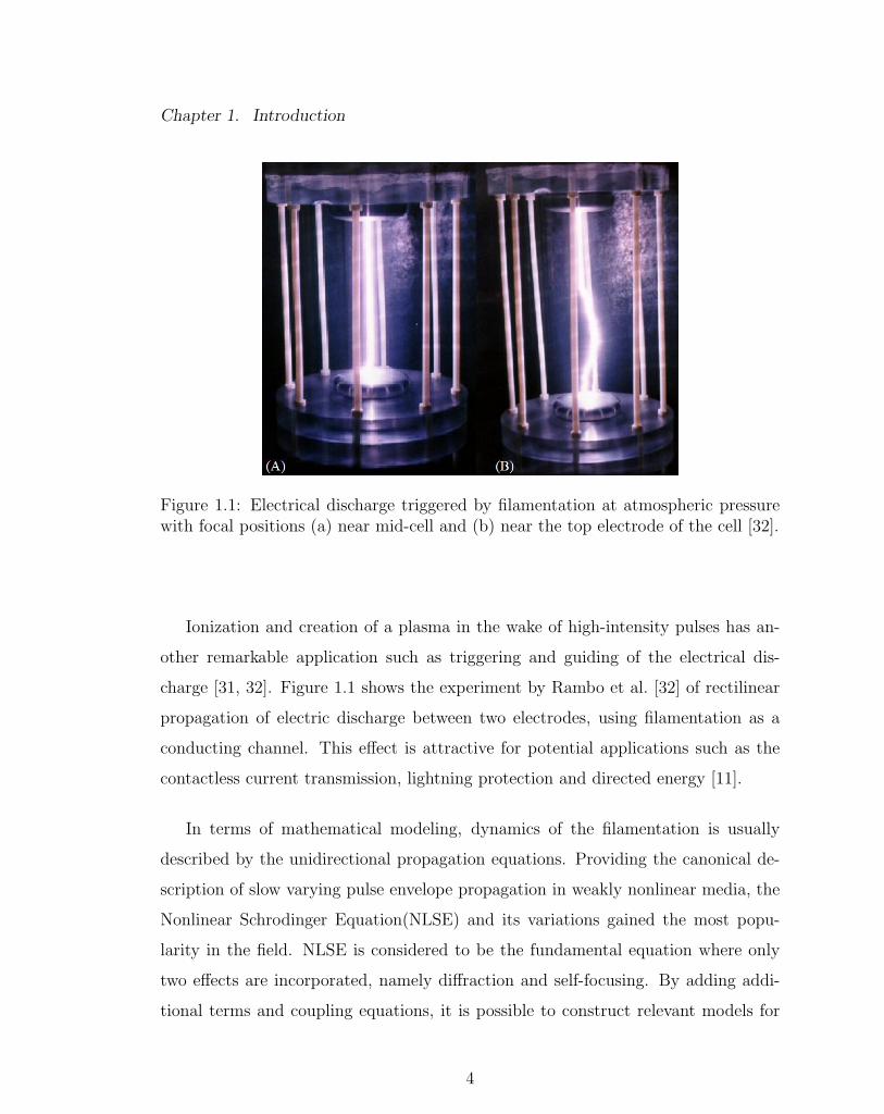
Figure 1.1: Electrical discharge triggered by filamentation at atmospheric pressurewith focal positions (a) near mid-cell and (b) near the top electrode of the cell [32].
Ionization and creation of a plasma in the wake of high-intensity pulses has an-
other remarkable application such as triggering and guiding of the electrical dis-
charge [31, 32]. Figure 1.1 shows the experiment by Rambo et al. [32] of rectilinear
propagation of electric discharge between two electrodes, using filamentation as a
conducting channel. This effect is attractive for potential applications such as the
contactless current transmission, lightning protection and directed energy [11].
In terms of mathematical modeling, dynamics of the filamentation is usually
described by the unidirectional propagation equations. Providing the canonical de-
scription of slow varying pulse envelope propagation in weakly nonlinear media, the
Nonlinear Schrodinger Equation(NLSE) and its variations gained the most popu-
larity in the field. NLSE is considered to be the fundamental equation where only
two effects are incorporated, namely diffraction and self-focusing. By adding addi-
tional terms and coupling equations, it is possible to construct relevant models for
4

Chapter 1. Introduction
many propagation regimes. The validity of such models may break down as the pulse
nears the collapse due to applicability restrictions to small amplitudes [33]. Although
equations based on NLSE typically are not integrable in dimensions more than one,
there are number of numerical methods that can be applied to find solutions. As
a rule, (2+1)D models don’t require heavy computational resources for integration
over a few meters. To catch the full dynamics of the pulse in (3+1)D case, parallel
computations can be used. Results from numerical simulations and experimental
data have been shown to be in sufficient agreement.
Currently several groups are working in the area of ultrashort high-intensity laser
pulses. Big contributions into the research came from the project called Teramo-
bile organized in 1999 by the group of five laboratories located in Berlin, Dresden
(Germany), Lyon, Palaiseau (France) and Geneva (Switzerland). They developed a
unique mobile laser system based on the chirped pulse amplification technique that
produces femtosecond pulses with peak power of a few terawatts [12].
Filamentation was observed in several experiments with femtosecond (fs) pulses
in both infrared (IR) and ultraviolet (UV) wavelengths. Comparing the two regimes,
it was detected that the IR filaments were obtained at much higher intensity but
at shorter pulse duration than the UV [34]. A few ps UV pulses were the longest
for which filamentation was found. The upper bound for the length of the pulse
that can produce filament is determined by the time necessary for electrons to gain
ionization energy of oxygen due to the inverse Bremsstrahlung. Plasma heating at
this time results in breakdown of air. For IR filaments with a 100 µm diameter it
happens around 1 ps. Since the rate of heating of electron plasma is proportional to
the wavelength and intensity, filaments can potentially be produced with longer UV
pulses.
High power UV pulses are especially interesting for long propagation. According
to [35], UV filament loses only about 30-40 µJ per meter. This is much less than
5

Chapter 1. Introduction
the nonlinear losses of IR filaments. By increasing pulse duration, the UV filaments
created can be longer(possibly even of the order of kilometers) and contain more
energy.
This dissertation is a theoretical examination of UV pulses of the duration of
the order of nanoseconds. An ongoing experiment at the University of New Mexico
has been conducted by professor Diels’ group. Nd:YAG laser oscillator-amplifier
system is utilized to generate pulses with quadrupled frequency. In order to obtain
long UV pulses with predetermined energy stimulated Brillouin scattering is used for
compression [36].
Figure 1.2: Experimental setup by Diels’ group
Due to the space limitations of the lab, measurements of propagation distance of
the filaments are bounded to the range of a few meters. The aerodynamic window, as
6

Chapter 1. Introduction
it seen on Figure 1.2, is a special device that was developed to stabilize the starting
position of the filament. Although generation of filaments using nanosecond pulses
with a few Joule of energy is still under construction, filamentation within 4 meters
from the aerodynamic window was observed using 200 ps pulses with energy 500 mJ
at 266 nm.
After the general introduction of this dissertation, chapter 2 provides the de-
tails of the mathematical model. Starting from Maxwell’s equations it shows the
derivation of the equation governing the nonlinear unidirectional propagation of a
slowly varying wavepacket envelope of a UV laser pulse. Formulation of the plasma
generation induced by the 3-photon ionization completes the model and the resulted
coupled equations are presented with defined physical quantities.
Chapter 3 begins with examining the stationary propagation model where time
dependence is neglected along with all possible losses. The nonlinear eigenvalue
problem is obtained from the steady state equation and a brief discussion of uniformly
distributed plane wave solutions is given. The chapter continues with the detailed
description of the numerical method that is used to find families of localized standing
filament profiles that vanish at infinity. With slight modification, the same method
is used to obtain vortex steady state solutions for different values of the topological
charge. These solutions are the main results of the chapter.
Chapter 4 addresses issues of stability of the localized solutions. The analysis
starts with a semi-analytical approach. Propagation equations of the beam width are
introduced using three different methods. The resulting equations are analyzed and
the implication on propagation is discussed. Then, linear stability analysis is formu-
lated and explored. This analysis includes the introduction of spatial perturbations,
the setup of the spectral problem and the verification of Vakhitov-Kolokolov criterion.
The discussion continues with the azimuthal instability of vortex stationary solutions
via derivation of the growth rate formula. The chapter ends with the analysis of the
7
Chapter 1. Introduction
spectral problem obtained from introducing spatiotemporal perturbations.
Chapter 5 describes numerical simulations of (2+1)D stationary and (3+1)D
non-stationary models. A discussion of the results is provided.
The description of the numerical method that is used in the propagation model
is given in Appendix A.
8

Chapter 2
The physical model
2.1 Derivation of propagation equation.
Since light is a form of electromagnetic field, we start our modeling with the
classical theory based on Maxwell’s equations [37, 38]
Gauss’ law for electricity: ∇ · ~D = ρ (2.1)
Gauss’ law for magnetism: ∇ · ~B = 0 (2.2)
Faraday’s law: ∇× ~E = −∂~B
∂t(2.3)
Ampere-Maxwell law: ∇× ~H =∂ ~D
∂t+ ~J (2.4)
where ρ and ~J are the electric charge and current densities.
The flux densities ~D and ~B related to electric and magnetic fields ~E and ~H
through the complemented relations
9

Chapter 2. The physical model
~D = ε0~E + ~P (2.5)
~B = µ0~H + ~M (2.6)
where ~P and ~M are the induced electric and magnetic polarization, and ε0 and µ0
are the vacuum permittivity and vacuum permeability. For a nonmagnetic medium,
~M = ~0. Now, taking curl of equation (2.3), using identity (2.4),(2.5) and (2.6) we
obtain
∇×∇× ~E = − 1
c2
∂2 ~E
∂t2− µ0
∂2 ~P
∂t2− µ0
∂ ~J
∂t(2.7)
where 1/c2 = ε0µ0. On the left hand side we use the vector identity
∇×∇× ~E = ∇(∇ · ~E)−∇2 ~E = −∇2 ~E (2.8)
where ∇ · ~E = 0, by divergence free assumptions [39]. After substituting (2.8) into
(2.7) we have
∇2 ~E − 1
c2
∂2 ~E
∂t2= µ0
(∂2 ~P
∂t2+∂ ~J
∂t
). (2.9)
Air can be considered to be a centro-symmetric medium with linear index n0, where
inversion symmetry is also present. Because of that, the polarization field can be
expanded in power series of ~E with cubic being lowest order nonlinearity. The first
term in the series corresponds to the linear polarization ~PL. Nonlinear polarization
10
Chapter 2. The physical model
which is the rest of the expansion can be treated as a small perturbation to the linear
since |~PNL| << |~PL| [40].
In general, the linear polarization is related to the field through the dielectric
susceptibility
~PL = ε0
∫ ∞−∞
χ(1)(t− τ) ~E(x, y, z, τ)dτ (2.10)
while in the frequency domain, from the convolution theorem, is
~PL = ε0χ
(1)(ω)~E(ω). (2.11)
The linear refractive index is defined by n20(ω) = 1 + χ(1)(ω) and the wavenumber
by dispersion relation k(ω) = ωn(ω)/c. For further consideration we expand k(ω) in
the Taylor series about the carrier frequency ω0
k(ω) = k(ω0) + k′(ω0)(ω − ω0) +∞∑n=2
1
n!k(n)(ω0)(ω − ω0)n. (2.12)
It is assumed that the field represents a beam propagating in one direction, namely in
direction z. This is why in the slowly varying quasi-monochromatic approximation,
it is useful to separate the rapidly varying part of the electric field by writing it in
the form
~E(x, y, z, t) = e(E(x, y, z, t)ei(k0z−w0t) + c.c.) (2.13)
where e is the polarization unit vector, E is the slowly varying complex amplitude and
11

Chapter 2. The physical model
k0 = k(ω0). The concept of slowly varying amplitude E means that |∂E/∂z| << k0|E|
and |∂E/∂t| << ω0|E|.
The amplitude E , in turn, can be represented as a Fourier integral
E(x, y, z, t) =
∫ ∞−∞E(x, y, z, ω)e−iωtdω (2.14)
so the linear part (LP ) of equation (2.9) can be written in the form
LP = ei(k0z−w0t)
[(∂
∂z+ ik0
)2
E +4⊥E +
∫ ∞−∞
k2(ω0 + ω)E(ω)e−iωtdω
](2.15)
where 4⊥ stands for transverse laplacian. Using expansion (2.12) and keeping terms
up to second order, the following is obtained
LP = ei(k0z−w0t)
[∂2E∂z2
+ 2ik0∂E∂z
+4⊥E + 2ik0k′0
∂E∂t− (k′20 + k0k
′′
0 )∂2E∂t2
]. (2.16)
It is also convenient to write the equation in a frame moving with the group velocity
of the pulse. This can be achieved by making a transformation t → t − k′0z and
z → z. As for second derivatives
∂2E∂z2− k′20
∂2E∂t2
=
(∂
∂z− k′0
∂
∂t
)(∂
∂z+ k′0
∂
∂t
)E << E . (2.17)
The equation (2.16) can be reduced to
LP = ei(k0z−w0t)
[2ik0
∂E∂z
+4⊥E − k0k′′
0
∂2E∂t2
]. (2.18)
12

Chapter 2. The physical model
The nonlinear part (NP) of equation (2.9) consists of the nonlinear polarization and
current density that is driven by the optical field. Since ~PNL acts as perturbation
of ~PL, higher order terms of nonlinear polarization are neglected except the domi-
nant χ(3), which corresponds to the optical Kerr effect. Now, if it is assumed that
the response of the medium is instantaneous, then the nonlinear polarization can be
simplified to
~PNL = ε0χ(3)( ~E · ~E) ~E ' 2n0n2ε0I ~E. (2.19)
Here, n2 is the self-focusing index and I is the laser intensity, defined as I = n0
2η0|E|2,
where η0 =√µ0/ε0 is the characteristic impedance of the vacuum.
In general, χ(3) includes the contribution of molecular vibrations and rotations.
Although Raman contribution is important for ultrashort pulses, this is not the case
for this work which assumes long UV pulses.
The model of plasma formation includes both multiphoton ionization and losses
due to response of produced charges to the optical field. While IR pulses are re-
quired to have 8-10 photons to liberate the electron from a molecule, simultaneous
absorption of 3-4 photons for UV pulses is enough. Ionization potential of oxygen
is lower compared to nitrogen. Hence, we can neglect ionization of nitrogen, due to
the small contribution. It follows that the number of electrons in the plasma is small
relative to the number of neutral molecules.
Schwarz et al.[35] set up the time scale under which current research is defined.
While the upper limit was established by inverse Bremsstrahlung, the lower limit
was defined by the time of plasma creation. As a result, the range of pulses duration
to be considered is between a few to 200 nanoseconds. In this range we can neglect
13

Chapter 2. The physical model
a second ionizing mechanism which occurs due to plasma heating by the laser field.
The losses of plasma occur when free electrons attach to positive ions producing neu-
tral molecules of oxygen. Another loss term in the plasma evolution equation can
be included due to the attachment of electrons to neutral molecules. The equation
governing free electron generation takes the form
∂Ne
∂t= σ(3)N0I
3 − βepN2e − γNe (2.20)
where Ne is the density of the electron plasma, σ(3) the 3d order multiphoton ioniza-
tion coefficient, βep the recombination coefficient and γ the electron-oxygen attach-
ment coefficient.
To complete the model we need to examine current density ~J , which consists of
free electron density ~Je and additional ionization current ~JMPA, which stands for
multiphoton absorption, i.e.
~J = ~Je + ~JMPA. (2.21)
Following the photo-ionization theory, the electron plasma is considered as a fluid
and can be modeled through collective velocity ~ve
∂
∂t~ve = − e
me
~E − ν~ve (2.22)
where me is the electron mass, e the elementary charge and ν the electron collision
frequency [41, 42].
Since motion of plasma electrons occurs in the optical field with much lower fre-
quency than ω0, we can separate fast and slow oscillations and eliminate the fast part
14

Chapter 2. The physical model
vLF ' −eE
me(ν − iω0). (2.23)
Free electron current density ~Je = −eNe~ve can be also decomposed to fast and slow
oscillation terms, where the low frequency contribution is given by
∂
∂tJeLF ' −i
ω0e2NeE
me(ν − iω0)≈(
1− i νω0
)e2
me
NeE . (2.24)
The last approximation is due to the fact that ν << ω0. The current in (2.21),
which accounts for dissipation of power necessary for multiphoton ionization, can be
expressed through electric field [42]
∂
∂tJMPALF = −iβ
(3)k0n20
4µ0η20
|E|4E . (2.25)
If equations (2.9), (2.18),(2.19) and (2.20) are combined with equations (2.21),(2.24)
and (2.25) along with cancelation of ei(k0z−ω0t), we immediately get
2ik0∂E∂z
+∇2⊥E + k2
0
n2
η0
|E|2E +−k20
e2
meω20ε0n
20
(1− i νω0
)NeE + iβ(3)k0n
20
4η20
|E|4E = 0
and
∂Ne
∂t= σ(3)N0
n30
8η30
|E|6 − βepN2e − γNe. (2.26)
15
Chapter 2. The physical model
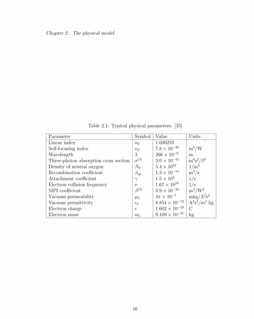
Table 2.1: Typical physical parameters. [35]
Parameter Symbol Value UnitsLinear index n0 1.000259Self-focusing index n2 7.8× 10⁻²³ m2/WWavelength λ 266× 10−9 mThree-photon absorption cross section σ(3) 3.0× 10−41 m6s2/J3
Density of neutral oxygen N0 5.4× 1024 1/m3
Recombination coefficient βep 1.3× 10⁻¹⁴ m3/sAttachment coefficient γ 1.5× 10⁸ 1/sElectron collision frequency ν 1.67× 10¹⁰ 1/sMPI coefficient β(3) 3.9× 10⁻³⁴ m3/W2
Vacuum permeability µ0 4π × 10−7 mkg/A2s2
Vacuum permittivity ε0 8.854× 10⁻¹² A2s4/m3 kgElectron charge e 1.602× 10⁻¹⁹ CElectron mass me 9.109× 10⁻³¹ kg
16

Chapter 3
Stationary solutions
3.1 The reduced model.
In the model derived in the previous chapter, UV filamentation is very sensitive
to the initial conditions. Since we are interested in answering the question about
the existence of pulses that maintain their shape over a long distance, this chapter
studies the stationary model. This means that all terms with time derivatives will
be dropped. Here, we consider the ideal case where all the loss terms are neglected
in the field envelope propagation equation, otherwise the beam would continuously
decrease due to the losses. The following equations are under consideration
2ik0∂E∂z
+∇2⊥E + k2
0
n2
η0
|E|2E − k20
e2
meω20ε0n
20
NeE = 0 (3.1)
σ(3)N0n3
0
8η30
|E|6 − βepN2e − γNe = 0. (3.2)
Based on experimental observations, equation (3.1) will be considered with assump-
17
Chapter 3. Stationary solutions
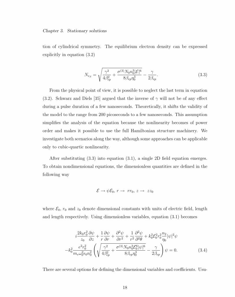
tion of cylindrical symmetry. The equilibrium electron density can be expressed
explicitly in equation (3.2)
NeS =
√γ2
4β2ep
+σ(3)N0n3
0|E|68βepη3
0
− γ
2βep. (3.3)
From the physical point of view, it is possible to neglect the last term in equation
(3.2). Schwarz and Diels [35] argued that the inverse of γ will not be of any effect
during a pulse duration of a few nanoseconds. Theoretically, it shifts the validity of
the model to the range from 200 picoseconds to a few nanoseconds. This assumption
simplifies the analysis of the equation because the nonlinearity becomes of power
order and makes it possible to use the full Hamiltonian structure machinery. We
investigate both scenarios along the way, although some approaches can be applicable
only to cubic-quartic nonlinearity.
After substituting (3.3) into equation (3.1), a single 2D field equation emerges.
To obtain nondimensional equations, the dimensionless quantities are defined in the
following way
E → ψE0, r → rr0, z → zz0
where E0, r0 and z0 denote dimensional constants with units of electric field, length
and length respectively. Using dimensionless variables, equation (3.1) becomes
i2k0r
20
z0
∂ψ
∂z+
1
r
∂ψ
∂r+∂2ψ
∂r2+
1
r2
∂2ψ
∂2θ+ k2
0E20r
20
n2
η0
|ψ|2ψ
−k20
e2r20
meω20ε0n
20
(√γ2
4β2ep
+σ(3)N0n3
0E60 |ψ|6
8βepη30
− γ
2βep
)ψ = 0. (3.4)
There are several options for defining the dimensional variables and coefficients. Usu-
18

Chapter 3. Stationary solutions
ally the electric field is normalized with respect to self focusing index and higher order
nonlinearities, so these quantities are defined in the following way
r0 =
(η0
k20E2
0n2
)1/2
, E0 =
(meω
20ε0n2
e2
√8n0βepη0
σ(3)N0
), z0 = 2k0r
20, µ =
γk20e
2r20
2βepmeω20ε0n
20
.
The equation (3.4) becomes
i∂ψ
∂z+
1
r
∂ψ
∂r+∂2ψ
∂r2+
1
r2
∂2ψ
∂2θ+ |ψ|2ψ − F (|ψ|2)ψ = 0 (3.5)
where F (|ψ|2) =√µ2 + |ψ|6 − µ, with µ = 4.6 or F (|ψ|2) = |ψ|3. From now on the
former function is defined as F1(|ψ|2) and the latter as F2(|ψ|2).
3.2 Nonlinear eigenvalue problem.
To construct a steady state solution, we look for a solution of the following
form ψ(r, θ, z) = ψ(r)eiΛz+imθ, where ψ(r) is real radially symmetric profile of am-
plitude, Λ > 0 is a propagation constant and m is an integer. Notice that Λ is
non-dimensional with the same scale as z. The substitution of the above ansatz into
the equation (3.5) yields a boundary value problem.
−Λψ +1
r
∂ψ
∂r+∂2ψ
∂r2− m2
r2ψ + ψ3 − F (ψ2)ψ = 0 (3.6)
ψ′(0) = 0, ψ(∞) = 0.
Equation (3.6) can be treated as an eigenvalue problem with eigenvalue Λ and eigen-
function ψ. First we concentrate on the fundamental ground state solution which
19

Chapter 3. Stationary solutions
does not carry any topological charge, i.e. m = 0 in (3.6). Then we will consider
stationary vortex solutions for different nonzero charges. The solutions ψ we look
for are localized in space, which later can be interpolated onto an xy-plane.
There are several methods that can be utilized to solve this boundary value
problem. One of them is the variational approach. This method uses trial function
in order to find the main characteristics of the beam, i.e. beam width and peak
amplitude. Although it provides relatively good explicit approximation, it has a
disadvantage of assuming that the solution has the shape of the predetermined trial
function.
The numerical approximation is another approach. Typically, boundary value
problems can be successfully solved by shooting or using finite difference methods.
The shooting method is known for its speed and adaptivity because it changes the
boundary value problem to the initial value problem (IVP). Unfortunately, it is not
as robust as the finite difference method because it can suffer from ill-conditioning of
the IVP. The choice was to employ the finite difference scheme along with Newton’s
iterations.
3.2.1 Plane wave solutions.
Before going into the discussion of radially dependent profiles, we consider the
simplest solutions of the given problem, which assume constant amplitude. These
solutions are called plane wave solutions
ψ = ψseiΛz+imθ. (3.7)
20

Chapter 3. Stationary solutions
Substituting (3.7) into equation (3.5), we derive an implicit form for the solution
−Λ− m2
r2+ ψ2
s − F (ψ2s) = 0.
Figure 3.1 shows example of solutions ψs(r = rm) of the above equation with mean
radius r1 = 4.5.
Figure 3.1: Plane wave solutions for m=1; (left)F (ψ2s) = F1(ψ2
s), (right)F (ψ2s) =
F2(ψ2s)
3.2.2 Fundamental solutions.
If F (ψ2) = 0, equation (3.6) becomes
−Λψ +1
r
∂ψ
∂r+∂2ψ
∂r2+ ψ3 = 0. (3.8)
21
Chapter 3. Stationary solutions
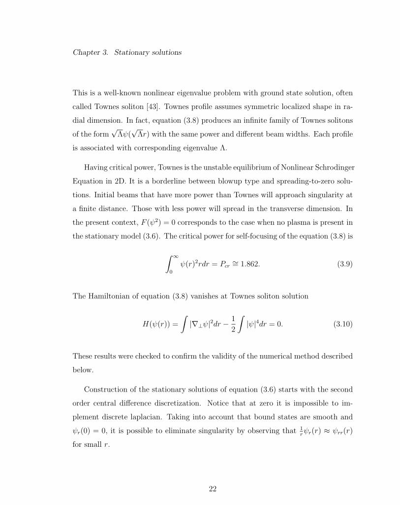
This is a well-known nonlinear eigenvalue problem with ground state solution, often
called Townes soliton [43]. Townes profile assumes symmetric localized shape in ra-
dial dimension. In fact, equation (3.8) produces an infinite family of Townes solitons
of the form√
Λψ(√
Λr) with the same power and different beam widths. Each profile
is associated with corresponding eigenvalue Λ.
Having critical power, Townes is the unstable equilibrium of Nonlinear Schrodinger
Equation in 2D. It is a borderline between blowup type and spreading-to-zero solu-
tions. Initial beams that have more power than Townes will approach singularity at
a finite distance. Those with less power will spread in the transverse dimension. In
the present context, F (ψ2) = 0 corresponds to the case when no plasma is present in
the stationary model (3.6). The critical power for self-focusing of the equation (3.8) is
∫ ∞0
ψ(r)2rdr = Pcr ∼= 1.862. (3.9)
The Hamiltonian of equation (3.8) vanishes at Townes soliton solution
H(ψ(r)) =
∫|∇⊥ψ|2dr −
1
2
∫|ψ|4dr = 0. (3.10)
These results were checked to confirm the validity of the numerical method described
below.
Construction of the stationary solutions of equation (3.6) starts with the second
order central difference discretization. Notice that at zero it is impossible to im-
plement discrete laplacian. Taking into account that bound states are smooth and
ψr(0) = 0, it is possible to eliminate singularity by observing that 1rψr(r) ≈ ψrr(r)
for small r.
22

Chapter 3. Stationary solutions
In the discrete form the equation at zero becomes
4 · ψ1 − ψ0
h2+ ψ3
0 − F (ψ20) = Λψ0 (3.11)
where due to the fact that the solution is radially symmetric, relation ψ1 = ψ−1 was
used.
In order to implement boundary condition at infinity, Townes asymptotic behav-
ior is assumed, i.e. ψ(r) ≈ ARr−1/2e−r, where AR ∼= 3.52, r 1. If the numerical
window is wide enough, it was observed that the value of the solution is substantially
small for large r. In this case, simply assigning zero to ψ(r) on the right boundary
also produces the same result.
To solve system of nonlinear equations, Newton’s iterations along with the con-
tinuation method are used. The continuation result will be used later in the stability
chapter. The numerical algorithm of Newton’s method was implemented with the
following scheme
Step1. Let (Λ, ψ(0)) be the initial guess, j = 0
Step2. while ||R(ψ(j))|| > tolerance
Step3. ψ(j+1) = ψ(j) − J(ψ(j))−1R(ψ(j))
Step4. j = j + 1
Step5. end
where tolerance = 10−7, J is the Jacobian matrix of R and function R(ψ) =
Aψ + f(ψ2), where
23

Chapter 3. Stationary solutions
A =1
h2
−4− Λ 4
12
−2− Λ 32
34
−2− Λ 54
2n−52n−4
−2− Λ 2n−32n−4
2n−32n−2
−2− Λ
and
f(ψ2) =
ψ3
0 − F (ψ20)ψ0
ψ31 − F (ψ2
1)ψ1
...
ψ3n−1 − F (ψ2
n−1)ψn−1
where n is the number of points on the grid. Notice that only the nonlinear part will
be updated at each iteration in the numerical implementation.
To obtain J(ψ(j))−1R(ψ(j)), the Thomas algorithm is applied. This is a proce-
dure that solves tridiagonal systems of linear equations by LU decomposition. This
algorithm requires only O(n) operations and doesn’t utilize storage for full n × n
matrix. The function in Matlab was defined as TRIDAG(a, b, c, R(ψ(j))) [44]. Here,
a, b and c are vectors containing subdiagonal, diagonal and superdiagonal elements
of J(ψ(j)).
For convergence of the iterations, it is crucial to choose an initial guess (Λ, ψ(r))
close enough to the solution. Although Gaussian is a relatively good approximation
of the Townes soliton, the guess was Townes in the form of a data vector that
24

Chapter 3. Stationary solutions
corresponds to appropriate Λ. After finding the first solution for the given Λ, this
solution is used as an initial guess in Newton’s iterations for Λ + h, where h is
a small quantity. It was observed that this continuation has the following range
Λ ∈ [0.01, 0.36] for F1 nonlinearity and Λ ∈ [0.01, 0.103] for F2. Figure 3.2 shows
stationary solution corresponding to Λ = 0.205 of F1 nonlinearity. Notice that steady
states are well approximated by gaussian beams.
Figure 3.2: Comparison between numerically obtained steady state profile(solid) atΛ = 0.205 and gaussian beam(dot-dashed) A2
0e−2r2/ω2
0 with power 400MW.
3.2.3 Vortex solutions.
Optical vortex represents a field that exhibits radial symmetry in the form a
ring and zero intensity at the center. In the stationary model (3.6), steady state
vortex solutions correspond to the case when topological charge m is nonzero.
The numerical approach of finding the stationary vortices is the same as for the
fundamental solution. The only difference is the discretization of the equation at
25

Chapter 3. Stationary solutions
zero. In the case of the vortex equation we have an additional term in the laplacian
that blows up at zero. Knowing that ψ(0) = 0, observe 1r2ψ(r) ≈ ψrr(r)
2when r is
small. Below is the difference equation corresponding to the zero boundary
(4 +m) · ψ1 − ψ0
h2+ ψ3
0 − F (ψ20) = Λψ0. (3.12)
Figure 3.3: Distribution of stationary vortex solutions for m = 1, 2, 3, 4 at Λ = 0.165
As an initial guess the stationary profile obtained from equation (3.8) is used.
As an example, for F1(|ψ|2) nonlinearity, convergence is observed on the interval
Λ ∈ [0.06, 0.44] form = 1. By increasing the numerical window it is possible to obtain
solutions with larger m. Figure 3.3 shows distribution of stationary vortex solutions
for F1 nonlinearity with four different topological charges. Notice that for larger m
the radius and power increase, thus making it harder to realize experimentally.
26

Chapter 3. Stationary solutions
Figure 3.4: Comparison of numerical solution(solid) form=1 and approximation(dot-dashed) A0re
−r2/ω20 , A0 = 0.33, ω0 = 4
27
Chapter 4
Stability analysis
Stability analysis of nonlinear waves is one of the most important issues in mod-
eling real physical experiments. Noise, turbulence, errors in measurements and other
small effects can contribute to deviations from the exact equilibrium. Usually direct
numerical computations are performed in order to compare theory with experiment,
but it is still not convincing without the analysis of stability properties against dif-
ferent perturbations.
The main goal of this chapter is to examine stability of the stationary ground-state
solutions found in the previous chapter. The analysis is divided into two parts. In the
first part of the chapter a semi-analytical approach is used. This approach doesn’t
exactly deal with the stationary solutions, but rather with gaussian approximations.
Some of the methods are limited to the stationary equation with cubic-quartic non-
linearity only. In the second part of the chapter, analysis is done directly to steady
states.
28

Chapter 4. Stability analysis
4.1 Semi-analytical approach.
Several semi-analytical methods can be used to study the ultrashort pulses in
the air. Here, a variational [45, 46, 47] and parabolic approximation methods [35] are
employed. The idea behind these methods is to describe the propagation of the main
characteristics of the beam by using an appropriate trial function. It is assumed
however, that the shape of the pulse profile is preserved, which imposes a limitation
on the produced models.
Simple evolution equations for the beam width and power are the results of
applying these methods. Although analysis based just on this equations may be
superficial, approximate evaluation of the beam propagation can be obtained.
4.1.1 Gaussian Trial Function.
This method will be applied to equation (3.5) with cubic-quartic nonlinearity.
The Lagrangian L corresponding to this problem is defined in the following way
L =i
2
(ψ∗∂ψ
∂z− ψ∂ψ
∗
∂z
)−∣∣∣∣∂ψ∂r
∣∣∣∣2 +1
2|ψ|4 − 2
5|ψ|5. (4.1)
A suitable trial function corresponding to gaussian beam is given by
ψ(r, z) = A(z)e−(
r2
ω2(z)+iC(z)r2+iφ(z)
)(4.2)
where parameters are amplitude A, beam width ω, wave curvature C and phase φ.
Substitution (4.2) into (4.1) produces
29

Chapter 4. Stability analysis
L = A2(r2C ′ + φ′)e−2r2/ω2 − 4A2r2
(1
ω4+ C2
)e−2r2/ω2
+1
2A4e−4r2/ω2
−2
5A5e−5r2/ω2
. (4.3)
After averaging over r, the reduced Lagrangian is given
< L >=
∫ ∞0
Lrdr = α1A2φ′ + α2A
2
(C ′ − 4
ω4− 4C2
)+ α3A
4 − α4A5 (4.4)
where α1(ω) = 2−2ω2, α2(ω) = 2−3ω4, α3(ω) = 2−4ω2 and α4(ω) = 5−2ω2.
To obtain Euler-Lagrange equations, the reduced Lagrangian is varied with re-
spect to the parameters A2, ω, φ and C.
Variation with respect to A2:
φ′ +ω2
2
(C ′ − 4
w4− 4C2
)+
1
2A2 − 2
5A3 = 0. (4.5)
Variation with respect to ω:
φ′ + ω2
(C ′ − 4
ω4− 4C2
)+
1
4A2 − 4
25A3 = 0. (4.6)
Variation with respect to φ:
∂
∂z
(ω2A2
)= 0. (4.7)
Variation with respect to C:
8ω4A2C +∂
∂z
(ω4A2
)= 0. (4.8)
30

Chapter 4. Stability analysis
Equation (4.7) gives the initial conditions on the beam waist and amplitude of the
gaussian function
A(z)ω(z) = const = A(0)ω(0). (4.9)
After using simple algebra, the final equation for the beam waist is obtained
d2ω
dz2=
16− 2A20ω
20
ω3+
48ω30A
30
25
1
ω4. (4.10)
Figure 4.1: Propagation of the width of 380MW gaussian beam.
Equation (4.10) is solved numerically using Matlab ODE45 solver. Figure 4.1
shows oscillatory behavior of the gaussian beam with power 380MW. The initial
conditions are taken from the gaussian approximation of the fundamental stationary
solution of equation (3.5) with F2(|ψ|2) nonlinearity that corresponds to Λ = 0.063.
31

Chapter 4. Stability analysis
Parabolic approximation method.
Despite similarity, the parabolic approximation method differs from the varia-
tional approach since a gaussian profile is substituted directly into the propagation
equation. Evolution equations are obtained after expansion of the gaussian into the
Taylor series near zero radius, making the main emphasis of this approach on the
center of the beam. Taking ansatz
ψ(r, z) = A0ω0
ω(z)e−(
r2
ω2(z)+i r2
2R(z)+iφ(z)
)(4.11)
into equation (3.5) with F1(|ψ|2) nonlinearity and using parabolic approximation
e−αr2ω2 = 1− α r
2
ω2(4.12)
two equations are obtained after keeping only leading order terms and equating real
and imaginary parts
2r2 w′(z)
w(z)3− w′(z)
w(z)− 2
R(z)+
4r2
w(z)2R(z)= 0 (4.13)
−1
2
r2R′(z)
R(z)2+ φ′(z)− 4
w(z)2+
4r2
w(z)4− r2
R(z)2+
A2
w(z)2− 2A2r2
w(z)4−√
µ2w(z)6 + A6
w(z)3+
3A6r2õ2w(z)6 + A6w(z)5
+ µ = 0. (4.14)
The beam waist evolution equation follows after combining the terms with r2 and
simple algebraic manipulations
32

Chapter 4. Stability analysis
d2w
dz2=
16− 8A20ω
20
w3(z)+
12A60ω
60
w4√µ2ω6 + A6
0ω60
. (4.15)
However, equation (4.15) is only approximately correct. If µ → ∞, equation
(3.5) becomes Nonlinear Schrodinger Equation and the second term on the right-
hand side of equation (4.15) is zero. Simple diagnostics shows that the critical power
for collapse event between NLSE and (4.15) differs by a factor 4. This can also
be observed comparing equations (4.10) and (4.15). To evade this inconsistency,
initial conditions are taken with A0/2 instead of A0. As shown in the figure 4.1 and
figure 4.2, the results are similar. Observed oscillations may be attributed to the
competition between self-focusing and plasma defocusing.
Figure 4.2: Evolution of the gaussian beam, with A0 = 1, ω0 = 1/√
0.12.
33

Chapter 4. Stability analysis
4.1.2 Ring Trial Function.
The variational approach is also applicable for the derivation of vortex beam
waist evolution equations. The Lagrangian L corresponding to the equation with
cubic-quartic nonlinearity includes azimuthal variable
L =i
2(ψ∗
∂ψ
∂z− ψ∂ψ
∗
∂z)−
∣∣∣∣∂ψ∂r∣∣∣∣2 − 1
r2
∣∣∣∣∂ψ∂θ∣∣∣∣2 +
1
2|ψ|4 − 2
5|ψ|5. (4.16)
A suitable trial function corresponding to the vortex beam problem has the following
form
ψ(r, z) = A(z)rme−(
r2
a2(z)+iC(z)r2+imθ+iφ(z)
). (4.17)
After averaging, the reduced Lagrangian can be expressed for any charge m
< L >= α1A2φ′ + α2A
2(C ′ − 4C2)− α3A2 − α4A
2 + α5A4 − α6A
5 (4.18)
where αi = αi(a) is listed below
α1 =
∫ ∞0
e−2r2
a2 r2m+1dr
α2 =
∫ ∞0
e−2r2
a2 r2m+3dr
α3 =
∫ ∞0
e−2r2
a2 r2m+1
(m
r− 2r
a
)2
dr
α4 = m2
∫ ∞0
e−2r2
a2 r2m−1dr
34
Chapter 4. Stability analysis
α5 =1
2
∫ ∞0
e−4r2
a2 r4m+1dr
α6 =2
5
∫ ∞0
e−5r2
a2 r5m+1dr.
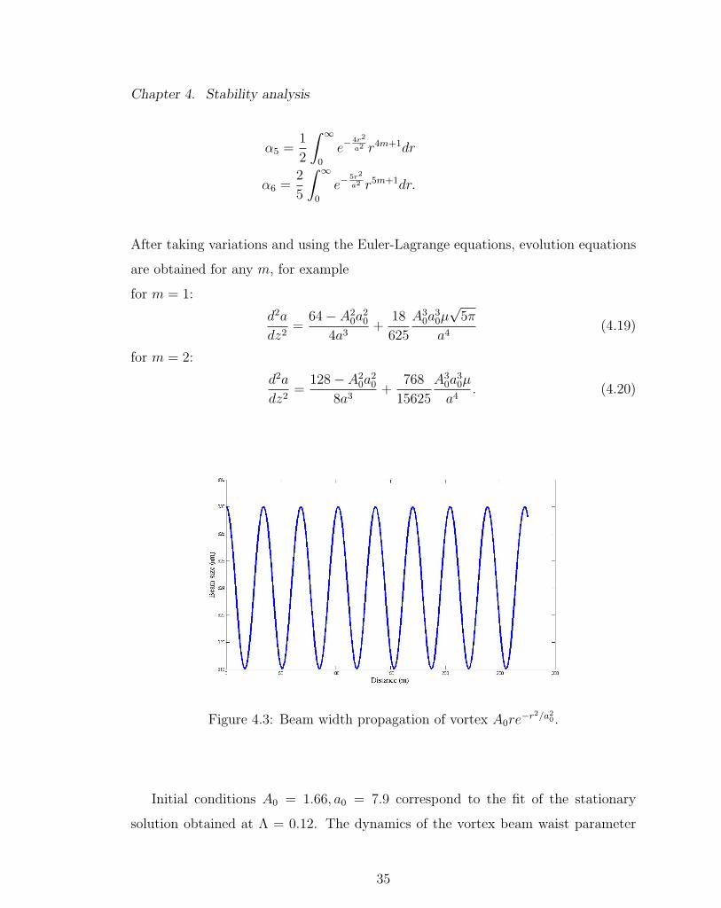
After taking variations and using the Euler-Lagrange equations, evolution equations
are obtained for any m, for example
for m = 1:
d2a
dz2=
64− A20a
20
4a3+
18
625
A30a
30µ√
5π
a4(4.19)
for m = 2:
d2a
dz2=
128− A20a
20
8a3+
768
15625
A30a
30µ
a4. (4.20)
Figure 4.3: Beam width propagation of vortex A0re−r2/a2
0 .
Initial conditions A0 = 1.66, a0 = 7.9 correspond to the fit of the stationary
solution obtained at Λ = 0.12. The dynamics of the vortex beam waist parameter
35
Chapter 4. Stability analysis
on the figure 4.3 shows periodic oscillations over hundreds of meters and increasing
oscillations after 600 meters, followed be infinite increase at around 1000. The cause
of this may be azimuthal instability.
4.2 Stability of stationary solutions.
Several methods of stability analysis that were developed in the nonlinear waves
theory can be applied to stationary localized solutions obtained in Chapter 3. Discus-
sions of different techniques are given by these authors [48, 49, 50, 51, 52, 53, 54, 55].
For equations of the Hamiltonian type, the variational method is usually the
standard approach. In this formulation, ground state solutions are stationary points
of the Hamiltonian H at fixed functional N =∫|ψ|2, which usually defines a beam
power. Stability follows if it can be shown that the bound state produces a mini-
mum of H. The absence of minimizers does not imply the instability of the states.
This analysis is sometimes called nonlinear because it doesn’t use the linearization
technique. This method is applied to the stationary problem with cubic-quartic
nonlinearity.
Another approach tackles the question of linear stability with respect to small
perturbations. In this case, stability of the stationary solution is assumed local in
contrast to absolute extremum of the Hamiltonian. This technique uses the lin-
earization of the equations on the background of ground state solution to study the
spectrum of differential operators.
Since dimensionality of the stationary solution is less than the dimensionality
of the initial problem, linear stability is divided into two parts. In the first part,
stability is examined with respect to small perturbations of the same dimensionality.
In the second part of analysis, stability of the stationary continuous wave is checked
36

Chapter 4. Stability analysis
against spatiotemporal perturbations.
4.2.1 Nonlinear stability.
Analysis starts with defining the Hamiltonian for cubic-quartic nonlinearity
H =
∫|4⊥ψ|2 −
1
2|ψ|4 +
2
5|ψ|5dxdy.
Following [33], assume that ψs(x, y) is the solution of
−Λψ +∇2⊥ψ + |ψ|2ψ − |ψ|3ψ = 0.
Now, let’s apply a transformation that preserves the power N
ψ(x, y) =1
aψ(xa,y
a
).
After substitution, the Hamiltonian has the following form
H(a) =1
a2
∫|4⊥ψ|2dxdy −
1
2
1
a2
∫|ψ|4dxdy +
2
5
1
a3
∫|ψ|5dxdy.
Since the ground state is a solution of the following variational problem δH+λ2N =
0 and N is preserved with varying a, it follows
∂H
∂a= − 2
a3M1 +
1
a3M2 −
6
5
1
a4M3 = 0
under the constraint a = 1. Here, M1 =∫|4⊥ψ|2dxdy, M2 =
∫|ψ|4dxdy, M3 =
37
Chapter 4. Stability analysis
∫|ψ|5dxdy and one can observe that all these quantities are positive, hence
M2 = 2M1 +6
5M3.
Stability can be determined from the sign of the second derivative of the Hamiltonian
∂2H
∂a2= 6M1 − 3M2 +
24
5M3 =
6
5M3 > 0.
This means that the ground state ψs is a minimum of H(a) and it is stable.
4.2.2 Spatial perturbations.
In the previous section, stability was addressed by means of the variational ap-
proach. However this method is not suitable for the equation (3.5) with F1(|ψ|2)
nonlinearity. In this case stability is investigated with respect to small spatial per-
turbations.
Consider the stationary localized solution obtained in chapter 3, ψ(x, y, z) =
ψs(x, y)eiΛz. Let’s perturb it and expand, keeping only the first order correction
ψ(x, y, z) ≈ (ψs(x, y) + u(x, y, z) + iv(x, y, z))eiΛz (4.21)
where u(x, y, z), v(x, y, z) are real functions. After substitution to the equation (3.4),
u, v satisfy the system
∂z
u
v
= N
u
v
38

Chapter 4. Stability analysis
where
N =
0 L0
−L1 0
and
L0 = −4⊥ + Λ− ψ2s − µ+
√µ2 + ψ6
s
L1 = −4⊥ + Λ− 3ψ2s − µ+
√µ2 + ψ6
s +6ψ6
s√µ2 + ψ6
s
are self-adjoint operators. If perturbations u, v are defined as feiκz and geiκz, the
system can be reduced to a single equation of the form
κ2f = L0L1f (4.22)
The goal of this analysis is to determine the sign of κ2. If it can be shown that κ2 > 0
for all bounded states, then (neutral) stability implies, otherwise the equilibrium
solution is unstable.
Let’s define operator G0 = −4⊥ + Λ− ψ2s . Then one can check that
G0 = − 1
ψs5 ·(ψ2s 5 (
1
ψs·))
hence
∫fL0fdxdy =
∫ ∣∣∣∣5( f
ψs
)∣∣∣∣2 ψ2sdxdy +
∫(−µ+
√µ2 + ψ6
s)f2dxdy ≥ 0
which means that the operator L0 is nonnegative, and it follows that for a solution
39

Chapter 4. Stability analysis
f , the minimum value of κ2 is given by
κ2m = min
< f |L1|f >< f |L−1
0 |f >
where < f |L|f >=∫fLfrdr. The sign of κ2
m is then determined by the numerator
µmin =< fL1f >. This in turn comes down to the spectral problem for L1, i.e.
L1f = σf + ρψs (4.23)
where σ and ρ are chosen to satisfy < f |f >= 1 and < f |ψs >= 0. Notice that if
equation (4.34) is multiplied by f from the left then the sign of µmin will be negative
depending on whether there is a solution of the spectral problem with σ < 0.
Functions f and ψs can be expanded in terms of orthogonal eigenfunctions ψn of
the operator L1 (L1ψn = λnψn). These series are substituted in equation (4.34) to
obtain
f = ρ∑ < ψs|ψn >
λn − σ. (4.24)
Equation (4.35) and the orthogonality constraint produces the following relation
S(σ) = ρ∑ < ψs|ψn >< ψn|ψs >
λn − σ. (4.25)
The sum does not contain zero eigenvalue and it has been proven [49] that operator L1
has only one negative eigenvalue. Hence when σ changes from negative to positive
eigenvalue, the function S(σ) changes from −∞ to +∞ passing zero. Therefore
the sign of σmin is determined by the sign of S(0). Since S(σ) is a monotonically
40

Chapter 4. Stability analysis
increasing function then S(0) < 0 means that S(σ) = 0 at some σ > 0 and vice
versa.
It follows from equations (4.35) and (4.36) that S(0) =< ψs|L−11 |ψs >. In order
to find S(0), the expression L0ψs = 0 is differentiated with respect to Λ. The result-
ing equation is written in the following form
L1∂ψs∂Λ
= −ψs.
Taking the inverse of L1 and multiplying both sides from the left by ψs the following
equation is obtained
S(0) = −1
2
∂P
∂Λ
where P =∫ψ2sdxdy.
Figure 4.4: Power of the steady state solution vs eigenvalues Λ.
41

Chapter 4. Stability analysis
The Vakhitov-Kolokolov criterion [48] states that the equilibrium solution is sta-
ble whenever dP/dΛ > 0 and unstable otherwise. As shown in figure 4.4, the power
is an increasing function of Λ, meaning that stability criterion is satisfied at least for
the range of the given values of Λ. If perturbations are only radial, the Vakhitov-
Kolokolov criterion can also be applied to the stationary vortex solutions. Figure
4.5 shows that localized vortices with different indices m are stable against such per-
turbations. This analysis however is not enough as ring-shaped solutions may suffer
from modulational instability in the azimuthal direction. The next section is devoted
to such problems.
Figure 4.5: Power of the steady state vortex solutions for m=1,2,3 vs eigenvalues Λ.
4.2.3 Azimuthal perturbations.
Azimuthal instability of optical vortices has been studied numerically in different
nonlinear media. It tends to split up the vortex into the set of fundamental solutions,
causing the symmetry to break. This was later shown experimentally [56].
42

Chapter 4. Stability analysis
The purpose of this section is to formulate and study the spectral problem that
emerges in the presence of the azimuthal perturbations. To begin, let’s perturb the
amplitude of the stationary solution ψ(r) by a function of the integer azimuthal
index L. Perturbations will be applied along the radius rm, which is defined as
r2m =
∫r2|ψm|2dr/Pm, where Pm is the power of the vortex
ψ(z, θ) =(ψs + a+e
−i(Lθ+λz) + a−ei(Lθ+λz)
)eiΛz+imθ. (4.26)
Here, ψs is assumed to be a constant intensity defined as ψs = ψs(r = rm) for some
fixed m. It can be seen from the setup that solution is unstable if λ has a nonzero
imaginary part and is stable otherwise. To find the instability growth rate, ansatz
(4.26) is plugged into the propagation equation (3.5). Two coupled equations are
obtained after linearization with respect to the perturbations
i(Λ− λ)a+ = −i(m− L)2
r2m
a+ + iBa+ + iCa− (4.27)
i(Λ + λ)a− = −i(m+ L)2
r2m
a− + iBa− + iCa+ (4.28)
where for F1(|ψ|2) :
B = 2ψ2s − (−µ+
√µ2 + ψ6
s)− 32
ψ6s√
µ2+ψ6s
, C = ψ2s − 3
2ψ6s√
µ2+ψ6s
and for F2(|ψ|2) :
B = 2ψ2s − 5
2ψ3s , C = ψ2
s − 32ψ3s .
The above equations can be rewritten in the matrix form
43

Chapter 4. Stability analysis
i
Λ− λ 0
0 −Λ− λ
a+
a−
= i
− (L−m)2
r2m+B C
−C (L+m)2
r2m−B
a+
a−.
The determinant is equated to zero to obtain
λ = −2Lm
r2m
±
√((L2 +m2)
r2m
+ Λ−B)2
− C2. (4.29)
To look for the growth rate, we need to look at the imaginary part of Λ
Im (λ) = Im
√((L2 +m2)
r2m
+ Λ−B)2
− C2. (4.30)
Figure 4.6: Growth rate of the stationary vortices as a function of the azimuthalindex L for different values of m=1,2,3
Figure 4.6 shows the instability growth rate for different charges m. Although
the index L is represented as a real parameter, it must be an integer in order to pre-
serve azimuthal periodicity. The maximum growth rate for m = 1 is approximately
44
Chapter 4. Stability analysis
attained at L = 3 and for m = 2 is at L = 5. Instability is bounded by larger number
L and the maximum growth rate is approximately at the same level for any m.
4.2.4 Spatiotemporal perturbations.
In order to investigate the time-perturbed solution, the plasma equation needs
to be nondimensionalized. It is done with the following transformation
Ne → Ne0Ne, t→ t0t.
The nondimensional equations are given
iψz +∇2⊥ψ + |ψ|2ψ −Ne(ψ)ψ = 0 (4.31)
∂Ne
∂t= |ψ|6 −N2
e − νNe (4.32)
where the additional normalization constants are defined in the following way
Ne0 =
√σN0n3
0
8η3βepE3
0 , t0 =1
βepNe0
, ν = γt0
Lets introduce the perturbation fields
ψ(z, r, t) = (ψs(r) + u(z, r, t) + iv(z, r, t))eiΛz+imθ (4.33)
Ne(z, r, t) = Nes(r) + δNe(z, r, t) (4.34)
45

Chapter 4. Stability analysis
where u, v, δNe ∝ exp(−iΩt+ iκz).
The main principle of this approach is to study the spectrum of the wave modes
along t-direction that are slightly different from the neutrally stable one (when Ω = 0
and κ = 0). This method was developed by Kuznetsov et al [51].
By putting the perturbed modes (4.43),(4.44) into equation (4.42) and using sim-
ple algebra, the result is
δNe =6ψ5
su
2Nes + ν − iΩ(4.35)
Substituting (4.43),(4.44) into (4.41), along with (4.45) and linearizing against the
background of a stationary solution, the coupled equations for perturbation fields
are obtained. They can be reduced to two independent equations
L0(L1 + δL)u = κ2u (4.36)
(L1 + δL)L0v = κ2v (4.37)
where L0 and L1 are operators from the section 4.3.2, and
δL =6ψ6
s√µ2 + ψ6
s − iΩ− 6ψ6
s√µ2 + ψ6
s
. (4.38)
In the case Ω = 0, it is clear that δL = 0 and equation (4.46-4.47) can be ex-
amined through Vakhitov-Kolokolov criterion. If Ω 6= 0, the spectrum of the given
46

Chapter 4. Stability analysis
spectral problem can be defined using perturbation expansion with neutrally stable
modes as the first approximation. By multiplying (4.48) from the left by rψs and
assuming v0 = rψs, it follows
κ2 =< ψsψsr|δL|ψsψsr > . (4.39)
The applicability criterion of this formula is the condition κ << Λ. Although insta-
bility is present for any Ω 6= 0, it follows directly from the setup of the equations
(4.46-4.47) that κ2 > 0 if Ω → ∞. Hence the growth rate decreases as Ω → ∞
and the maximum growth rate is determined by the equation (4.50). While it is
challenging to find an exact maximum, it is shown in figure 4.7 that the growth rate
is limited.
47

Chapter 4. Stability analysis
(a)
(b)
Figure 4.7: Growth rate vs Ω (a) fundamental solution at Λ=0.205, (b) m=1 vortexsolution at Λ=0.165
48

Chapter 5
Numerical simulations
This chapter provides numerical results using non-dimensional propagation mod-
els. In the first section the (2 + 1)D stationary model is integrated numerically. In
this case it is assumed that the pulse is long enough to be considered as a continu-
ous wave. In the second section, the beam is confined in time in order to produce
a finite pulse. Therefore the time dimension is included and the dynamics of the
non-stationary profiles are investigated in the more realistic (3 + 1)D problem. Last
section presents propagation of the pulse perturbed by random noise in the model
with included nonlinear losses. In all scenarios, propagation of the pulse is provided
by the Fourier split-step method which is detailed in Appendix A. The propagation
code was written in C and used the MPI library. The simulations were made on
a linux cluster (NANO) from the Center for Advanced Research Computing at the
University of New Mexico, which computational power expands up to 144 CPUs.
The results of the simulations were plotted using Matlab graphing utilities.
49
Chapter 5. Numerical simulations
5.1 (2+1)D simulations.
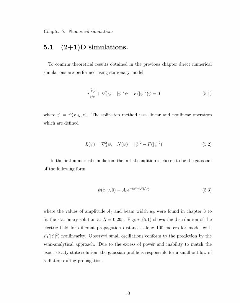
To confirm theoretical results obtained in the previous chapter direct numerical
simulations are performed using stationary model
i∂ψ
∂z+∇2
⊥ψ + |ψ|2ψ − F (|ψ|2)ψ = 0 (5.1)
where ψ = ψ(x, y, z). The split-step method uses linear and nonlinear operators
which are defined
L(ψ) = ∇2⊥ψ, N(ψ) = |ψ|2 − F (|ψ|2) (5.2)
In the first numerical simulation, the initial condition is chosen to be the gaussian
of the following form
ψ(x, y, 0) = A0e−(x2+y2)/ω2
0 (5.3)
where the values of amplitude A0 and beam width w0 were found in chapter 3 to
fit the stationary solution at Λ = 0.205. Figure (5.1) shows the distribution of the
electric field for different propagation distances along 100 meters for model with
F1(|ψ|2) nonlinearity. Observed small oscillations conform to the prediction by the
semi-analytical approach. Due to the excess of power and inability to match the
exact steady state solution, the gaussian profile is responsible for a small outflow of
radiation during propagation.
50

Chapter 5. Numerical simulations
(a) z=0 m (b) z=10.75 m
(c) z=32.27 m (d) z=53.78 m
(e) z=75.3 m (f) z=96.8 m
Figure 5.1: Propagation of gaussian beam A0e−(x2+y2)/ω2
0 with A0 = 1, ω0 = 1/√
0.12.
51
Chapter 5. Numerical simulations
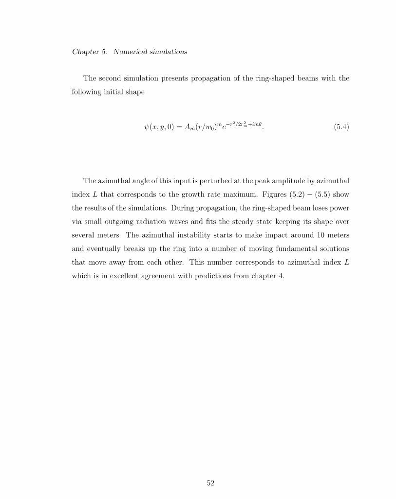
The second simulation presents propagation of the ring-shaped beams with the
following initial shape
ψ(x, y, 0) = Am(r/w0)me−r2/2r2m+imθ. (5.4)
The azimuthal angle of this input is perturbed at the peak amplitude by azimuthal
index L that corresponds to the growth rate maximum. Figures (5.2) − (5.5) show
the results of the simulations. During propagation, the ring-shaped beam loses power
via small outgoing radiation waves and fits the steady state keeping its shape over
several meters. The azimuthal instability starts to make impact around 10 meters
and eventually breaks up the ring into a number of moving fundamental solutions
that move away from each other. This number corresponds to azimuthal index L
which is in excellent agreement with predictions from chapter 4.
52

Chapter 5. Numerical simulations
(a) z=0 m
(b) z=10.76 m
(c) z=21.5 m
Figure 5.2: Vortex propagation m=1, L = 3
53

Chapter 5. Numerical simulations
(a) z=32.26 m
(b) z=43.03 m
(c) z=53.78 m
Figure 5.3: Vortex propagation m = 1, L = 3
54

Chapter 5. Numerical simulations
(a) z=0 m
(b) z=9.84 m
(c) z=19.68 m
Figure 5.4: Vortex propagation m = 2, L = 5
55

Chapter 5. Numerical simulations
(a) z=39.37 m
(b) z=59.05 m
(c) z=78.74 m
Figure 5.5: Vortex propagation m = 2, L = 5
56
Chapter 5. Numerical simulations
5.2 (3+1)D simulations.
The equations of the (3+1)D model are given
iψz +∇2⊥ψ + |ψ|2ψ −Ne(ψ)ψ = 0 (5.5)
∂Ne
∂t= |ψ|6 −N2
e − νNe (5.6)
where ψ = ψ(x, y, z, t) and Ne = Ne(x, y, z, t).
Integration starts with the assumption that no plasma is present at the posi-
tion z = 0. After evaluation of the electric field at the next propagation step,
plasma density is numerically computed from the equation (5.6) using the fourth-
order RungeKutta method
Nen+1 = Nen +1
6(K1 + 2K2 + 2K3 +K4)
tn+1 = tn + ∆t,
K1 = ∆tf(tn, Nen),
K2 = ∆tf
(tn +
1
2∆t, Nen +
1
2K1
),
K3 = ∆tf
(tn +
1
2∆t, Nen +
1
2K2
),
K4 = ∆tf(tn + ∆t, Nen +K3),
where f(tn, Nen) = |ψ(zm, tn)|6 −N2en − νNen , zm = m∆z.
To create a nanosecond pulse the following initial conditions are used
ψ(x, y, 0, t) = ψ(x, y, 0)e−t2/t2p (5.7)
57

Chapter 5. Numerical simulations
where ψ(x, y, 0) is the 2D initial condition from previous section.
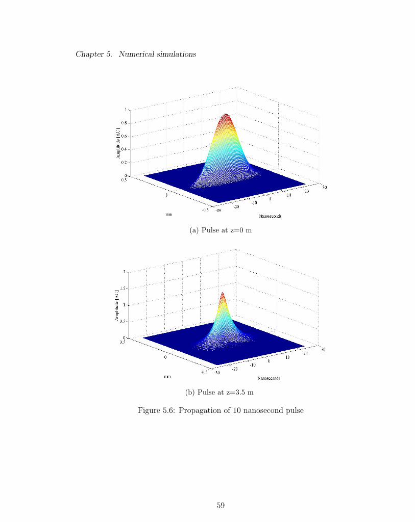
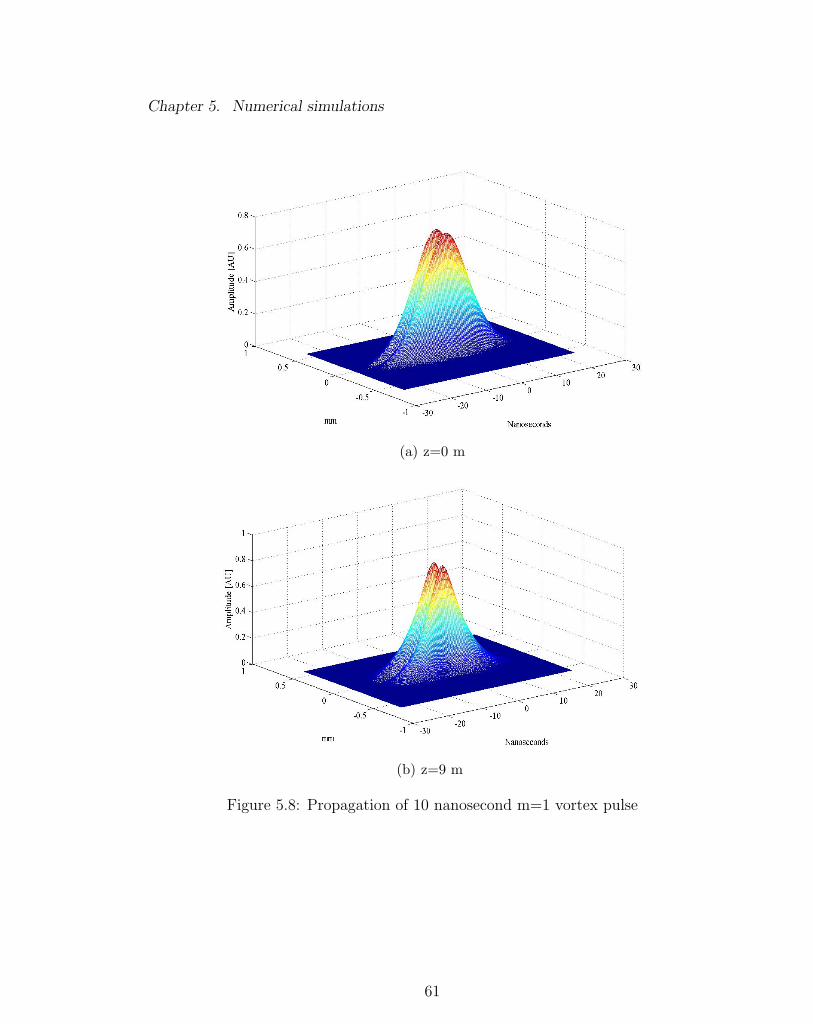
The results of the simulations are shown on Figures (5.6) − (5.9). Dynamics of
the nanosecond pulse differ from the small oscillations around equilibrium of the
stationary model predicted by the theory. Propagation develops into the collapse
event, as a pulse of a finite temporal duration is not exact steady state. Exact
distance at which regularization of the collapse is attained is unknown due to the
inability to capture further increase of the amplitude with the current uniform grid.
5.3 Numerical tests and convergence.
To check the validity of the results, several tests were employed. First, it was
observed that the power and the energy of the pulse stay conserved during propaga-
tion within 0.01% of accuracy. In (2+1)D model, the tests were done at the distances
where the radiation outflow is negligible. The loss of power further is attributed to
the absorbtion of the radiation waves on the boundaries, by removing corresponding
frequencies in the Fourier domain.
To verify the error convergence, simulations were done for different values of h and
∆t. Number of points in the computational grids were chosen among 128, 256, 512
in each direction. When h was divided by two, ∆z was divided by four, in order to
eliminate the growth of the numerical instability.
Another test checks the convergence of the plasma density to the steady state
solution in the equation (5.6) for various values of ∆t. Finally, initial condition
(5.3) was used in the (3+1)D model in order to check the stability of the stationary
solution under the current numerical scheme. It was observed that the growth of the
numerical errors eventually destroys stability for large values of z.
58
Chapter 5. Numerical simulations
(a) Pulse at z=0 m
(b) Pulse at z=3.5 m
Figure 5.6: Propagation of 10 nanosecond pulse
59

Chapter 5. Numerical simulations
(a) Pulse at z=7.5 m
(b) Pulse at z=10 m
Figure 5.7: Propagation of 10 nanosecond pulse
60
Chapter 5. Numerical simulations
(a) z=0 m
(b) z=9 m
Figure 5.8: Propagation of 10 nanosecond m=1 vortex pulse
61

Chapter 5. Numerical simulations
(a) z=16.5 m
(b) z=22 m
Figure 5.9: Propagation of 10 nanosecond m=1 vortex pulse.
62

Chapter 5. Numerical simulations
5.4 (3+1)D model with nonlinear losses.
In the final simulation, the equation (5.5) is considered with the nonlinear losses
iψz +∇2⊥ψ + |ψ|2ψ − (1− iε1)Ne(ψ)ψ + iε2|ψ|4ψ = 0 (5.8)
∂Ne
∂t= |ψ|6 −N2
e − νNe (5.9)
where ε1 = 2.36× 10⁻⁶ and ε2 = 5.32× 10⁻⁵.
To check the spatiotemporal instability result, the initial conditions are taken to
be the same as from the previous section which are then perturbed by a 1% random
noise in temporal direction.
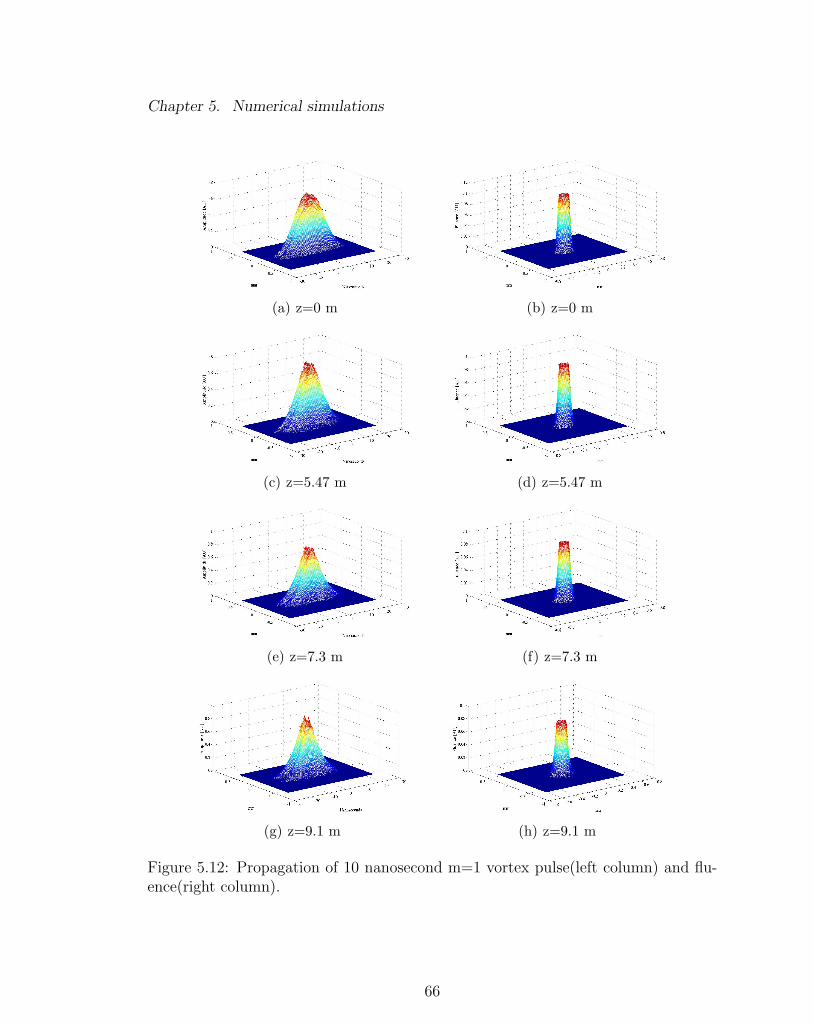
Figures (5.10)− (5.13) show the propagation of the pulse profile and the fluence
of the pulse which corresponds to the energy per unit area. Fluence is computed
numerically in the following way:
F (x, y, z) =
∫ ∞−∞|ψ(x, y, z, t)|2dt (5.10)
This simulation confirms the theoretical prediction that the pulse of the order
of nanoseconds suffers from the modulational instability. Temporal perturbations
become significant after several meters. Collapse event accelerates the noise growth.
It was observed that beams with less intensity have longer unaffected propagation,
since the collapse event develops longer.
63

Chapter 5. Numerical simulations
(a) z=0 m (b) z=0 m
(c) z=1.25 m (d) z=1.25 m
(e) z=2 m (f) z=2 m
(g) z=2.5 m (h) z=2.5 m
Figure 5.10: Propagation of 10 nanosecond pulse(left column) and fluence(right col-umn)
64

Chapter 5. Numerical simulations
(a) z=3 m (b) z=3 m
(c) z=3.5 m (d) z=3.5 m
(e) z=4 m (f) z=4 m
(g) z=4.5 m (h) z=4.5 m
Figure 5.11: Propagation of 10 nanosecond pulse(left column) and fluence(right col-umn)
65
Chapter 5. Numerical simulations
(a) z=0 m (b) z=0 m
(c) z=5.47 m (d) z=5.47 m
(e) z=7.3 m (f) z=7.3 m
(g) z=9.1 m (h) z=9.1 m
Figure 5.12: Propagation of 10 nanosecond m=1 vortex pulse(left column) and flu-ence(right column).
66

Chapter 5. Numerical simulations
(a) z=10.94 m (b) z=10.94 m
(c) z=12.76 m (d) z=12.76 m
(e) z=14.58 m (f) z=14.58 m
(g) z=16.4 m (h) z=16.4 m
Figure 5.13: Propagation of 10 nanosecond m=1 vortex pulse(left column) and flu-ence(right column).
67

Chapter 6
Conclusion
This dissertation studies the theoretical possibility of the propagation of high in-
tensity UV filaments and vortices in air. The governing system of equations were
derived and non-dimentionalized. It was shown by Newton’s iteration method that
the steady state model produces localized radially symmetric solutions for certain
range of eigenvalues Λ. It was observed that fundamental stationary solutions can
be well approximated by elementary functions, for example in the case of m = 0 they
can be approximated by gaussian.
The stability of obtained stationary solutions is divided into two parts. First we
use semi-analytical approach to study the dynamics of the beam width. The results
show stable although oscillatory behavior of the stationary solutions. Then, the linear
stability of the radial profiles is investigated. In this case, it was proven by Vakhitov-
Kolokolov criterion that the fundamental as well as vortex steady state solutions
are stable against spatial perturbations. It was shown that vortex solutions suffer
from instability against azimuthal perturbations. In the last part of the chapter 4,
spatiotemporal perturbations were applied to full time dependent problem. Analysis
of the spectral problem shows that the equilibria of the given model are inherently
68

Chapter 6. Conclusion
unstable against temporal perturbations.
Theoretical predictions are consistent with the numerical simulations only if the
model assumes long enough pulse to be considered as a continuous wave. Based on
the above analysis, the given model predicts that it’s possible for UV filaments and
vortices to propagate over several meters, even tens of meters before the modulational
instability becomes significant to affect the propagation.
69

Appendix A
Numerical integration scheme
For simulations along the propagation direction a split-step spectral method is
used. To describe this method it is convenient to consider the field equation in the
following form
∂ψ
∂z= iL(ψ)ψ + iN(ψ)ψ (A.1)
where L(ψ) is a linear part of the equation, and N(ψ) is nonlinear. The field ad-
vances from one propagation step to another according to the following expression
ψ(·, z + ∆z) ≈ exp(i∆z(L+N(ψ)))ψ(·, z). (A.2)
There exists several different splitting procedures of the right-hand side of (A.2).
The approach is chosen to be of the second order of accuracy which was introduced
by Strang [57].
exp(i∆z(L+N(ψ))) ≈ exp(i∆zL/2) exp(i∆zN(ψ)) exp(i∆zL/2). (A.3)
70
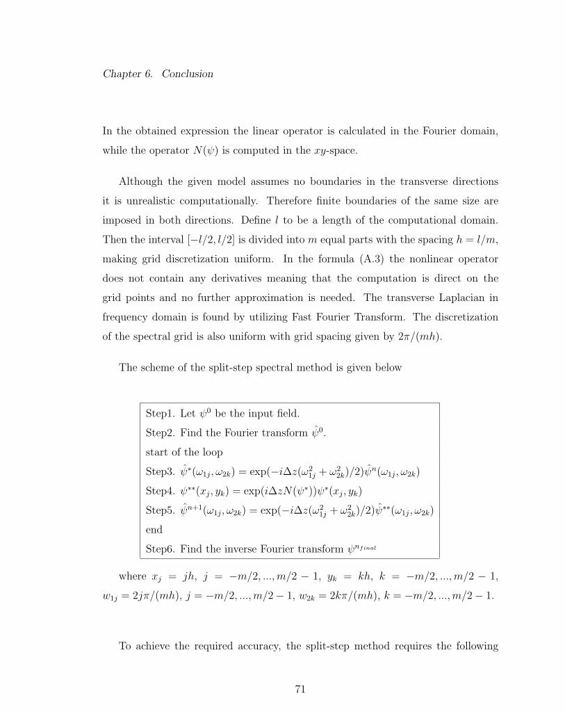
Chapter 6. Conclusion
In the obtained expression the linear operator is calculated in the Fourier domain,
while the operator N(ψ) is computed in the xy-space.
Although the given model assumes no boundaries in the transverse directions
it is unrealistic computationally. Therefore finite boundaries of the same size are
imposed in both directions. Define l to be a length of the computational domain.
Then the interval [−l/2, l/2] is divided into m equal parts with the spacing h = l/m,
making grid discretization uniform. In the formula (A.3) the nonlinear operator
does not contain any derivatives meaning that the computation is direct on the
grid points and no further approximation is needed. The transverse Laplacian in
frequency domain is found by utilizing Fast Fourier Transform. The discretization
of the spectral grid is also uniform with grid spacing given by 2π/(mh).
The scheme of the split-step spectral method is given below
Step1. Let ψ0 be the input field.
Step2. Find the Fourier transform ψ0.
start of the loop
Step3. ψ∗(ω1j, ω2k) = exp(−i∆z(ω21j + ω2
2k)/2)ψn(ω1j, ω2k)
Step4. ψ∗∗(xj, yk) = exp(i∆zN(ψ∗))ψ∗(xj, yk)
Step5. ψn+1(ω1j, ω2k) = exp(−i∆z(ω21j + ω2
2k)/2)ψ∗∗(ω1j, ω2k)
end
Step6. Find the inverse Fourier transform ψnfinal
where xj = jh, j = −m/2, ...,m/2 − 1, yk = kh, k = −m/2, ...,m/2 − 1,
w1j = 2jπ/(mh), j = −m/2, ...,m/2− 1, w2k = 2kπ/(mh), k = −m/2, ...,m/2− 1.
To achieve the required accuracy, the split-step method requires the following
71

Chapter 6. Conclusion
condition to be satisfied [58]
∆z ≤ 2h2
π2. (A.4)
72

References
[1] G. Mourou. The ultrahigh-peak-power laser: present and future. Appl. Phys. B65, 205211, 1997.
[2] D. Strickland, G. Mourou. Compression of amplified chirped optical pulses. Op-tic Communications, vol. 56, No. 3, Dec. 1, pp. 219-221, 1985.
[3] P. Maine, D. Strickland, P. Bado, M. Pessot, G. Mourou. Generation of ultrahighpeak power pulses by chirped pulse amplification. IEEE J. Quantum Electron.24, 398-403, 1988.
[4] A. Braun, G. Korn, X. Liu, D. Du, J. Squier, G. Mourou. Self-channeling ofhigh-peak-power femtosecond laser pulses in air. Opt. Lett. 20(1), 73-75, 1995.
[5] A. Brodeur, C. Chen, C. Ilkov, S. Chin, O. Kosareva, V. Kandidov. Movingfocus in the propagation of ultrashort laser pulses in air. Opt.Lett. 22(5), 304-306, 1997.
[6] E. Nibbering, P. Curley, G. Grillon, B. Prade, M. Franco, F. Salin, A. Mysy-rowicz. Conical emission from self-guided femtosecond pulses in air. Opt. Lett.21(1),62-64, 1996.
[7] Z. Jin, J. Zhang, M.H. Lu, Y.T. Li, Z.H. Wang, Z.Y. Wei, X.H. Yuan, W. Yu.Control of filamentation induced by femtosecond laser pulses propagating in air.Optics Express 10424, Vol. 13, No. 25, Dec. 2005.
[8] Z-Q Hao, J. Zhang, X. Lu, T-T Xi, Y-T Li, X-H Yuan, Z-Y Zheng, Z-H Wang,W-J Ling, Z-Y Wei. Spatial evolution of multiple filaments in air induced byfemtosecond laser pulses. Optics Express 773, Vol. 14, No. 2, Jan 2006.
[9] V. Talanov. Self-focusing of electromagnetic waves in nonlinear media. Izv.Vysshikh Uchebn. Zavedenii Radiofiz 7, 564-565, 1964.
73

References
[10] V. Talanov Self-focusing of wave beams in nonlinear media. JETP Lett. 2(5),138, 1965.
[11] J.Kasparian, J-P Wolf. Physics and applications of atmospheric nonlinear opticsand filamentation. Optics express 466, Vol. 16, No. 1, 2008.
[12] A. Couairon, A. Mysyrowicz. Femtosecond filamentation in transparent media.Physics Reports 441, 47 189, 2007.
[13] L. Berge. Wave collapse in physics: principles and applications to light andplasma waves. Physics Reports, 303:259370, 1998.
[14] K.D. Moll, A.L. Gaeta, G. Fibich. Self-Similar Optical Wave Collapse: Obser-vation of the Townes Profile. Physical Review Letters, Vol. 90, No. 20, May2003.
[15] Gadi Fibich, Shmuel Eisenmann, Boaz Ilan, Yossi Erlich, Moshe Fraenkel, ZoharHenis, Alexander L. Gaeta and Arie Zigler. Self-focusing distance of very highpower laser pulses. Optics Express Vol. 13, No. 15, 5898, 25 July 2005.
[16] J-C Diels, W. Rudolph. Ultrashort Laser Pulse Phenomena. Second Edition,Academic Press, 2006.
[17] A. Couairon, L. Berge. Light filaments in air for ultraviolet and infrared wave-length. Physical Review Letters, 88(13):135003, Mar 2002.
[18] E. Arevalo. Self-focusing arrest of femtosecond laser pulses in air at differentpressures. Physical Review E 74, 016602, 2006.
[19] M. Mlejnek, E.M. Wright, J.V. Moloney. Dynamic spatial replenishment of fem-tosecond pulses propagating in air. Optics Letters 382, Vol. 23, No. 5, March1998.
[20] V. Skarka, N.B. Aleksic, V.I. Berezhiani. Evolution of singular optical pulsestowards vortex solitons and filamentation in air. Physics Letters A, p.1-8, Oct.2003.
[21] A. Vincotte and L. Berge, Femtosecond Optical Vortices in Air. Phys. Rev. Lett.95, 193901, 2005.
[22] M. Kolesik, J. Moloney. Self-healing femtosecond light filaments. Opt. Lett.29(6), 590-592, 2004.
[23] F. Courvoisier, V. Boutou, J. Kasparian, E. Salmon, G. Mejean, J. Yu, J. Wolf.Ultraintense light filaments transmitted through clouds. Appl. Phys. Lett. 83(2),213-215, 2003.
74
References
[24] A. Dubietis, E. Kucinskas, G. Tamosauskas, E. Gaizauskas, M. Porras, P. DiTrapani. Self-reconstruction of light filaments. Opt. Lett. 29, 2893-2895, 2004.
[25] G. Mechain, C. D’Amico, Y. Andre, S. Tzortzakis, M. Franco, B. Prade, A.Mysyrowicz, A. Couairon, A. Salmon, R. Sauerbrey. Length of plasma filamentscreated in air by a multiterawatt femtosecond laser. Opt. Commun. 247,171-180,2005.
[26] G. Matvienko, V. Veretennikov, G. Krekov, M. Krekova. Remote sensing ofatmospheric aerosols with a white-light femtosecond lidar. Atmos. Oceanic Opt.16, 1013-1019, 2003.
[27] E. Frejafon, J. Kasparian, P. Rambaldi, B. Vezin, V. Boutou, J. Yu, M. Ulbricht,D. Weidauer, B. Ottobrini, E. de Saeger, B. Kramer, T. Leisner, P. Rairoux, L.Woste, J-P Wolf. Laser applications for atmospheric pollution monitoring. Eur.Phys. J. D 4, 231, 1998.
[28] J. Kasparian, M. Rodriguez, G. Mejean, J. Yu, E. Salmon, H. Wille, R.Bourayou, S. Frey, Y-B Andre, A. Mysyrowicz, R. Sauerbrey, J-P Wolf, L.Woste. White light filaments for atmospheric analysis. Science 301,61, 2003.
[29] K. Stelmaszczyk, P. Rohwetter, G. Mejean, J. Yu, E. Salmon, J. Kasparian,R. Ackermann, J-P Wolf, L. Woste. Long-distance remote laser-induced break-down spectroscopy using filamentation in air. Appl. Phys.Lett. 85(18), 3977-3979, 2004.
[30] P. Rohwetter, J. Yu, G. Mejean, K. Stelmaszczyk, E. Salmon, J. Kasparian, J-PWolf, L. Woste. Remote LIBS withultrashort pulses: characteristics in picosec-ond and femtosecond regimes. J. Anal. At. Spectrom. 19, 437-444, 2004.
[31] Xin Miao Zhao, Jean-Claude Diels, Cai Yi Wang, and Juan M. Elizondo. Fem-tosecond ultraviolet laser pulse induced lightning discharges in gases. IEEE Jour-nal of Quantum Electronics, 31:599612, 1995.
[32] P. Rambo, J. Schwarz, J-C Diels. High-voltage electrical discharges induced byan ultrashort-pulse UV laser system. J. Opt. A: Pure Appl. Opt. 3 146-158,2001.
[33] C.Sulem, P.L.Sulem. The Nonlinear Scrodinger Equation, Self-focusing andWave Collaspe. Applied Mathematical Science, Springer-Verlag, New York Inc,1999.
[34] J. Schwarz, P. Rambo, J-C Diels, M. Kolesik, E. Wright, J. Moloney. Ultravioletfilamentation in air. Optics Comm. 180, 383-390, 2000.
75
References
[35] J. Schwarz, J-C Diels. Analitical solution for uv filaments. Physical Review A,vol. 65, 013806, 2001.
[36] O. Chalus, A. Sukhinin, A. Aceves, J-C Diels. Propagation of non-diffractionintense ultraviolet beams. Optics Communications 281, 3356-3360, 2008.
[37] R.W. Boyd. Nonlinear Optics, Second Edition. Academic Press, 2003.
[38] Y. Shen. The Principles of Nonlinear Optics. Wiley-Interscience, New York,1984.
[39] N.N. Akhmediev, A. Ankiewicz. Solitons, Nonlinear pulses and beams. Chapman& Hall, 1997.
[40] Y.S. Kivshar, G.P. Agrawal. Optical Solitons, From Fibers to Photonic Crystals.Academic Press, 2003.
[41] A. Couairon, L. Berge. Modeling the filamentation of ultra-short pulses in ion-izing media. Physics of Plasmas, Vol. 7, No. 1, Jan. 2000.
[42] S.Skupin, L.Berge. Self-guiding of femtosecond light pulses in condensed media:Plasma generation versus chromatic dispersion. Physica D 220, 14-30, 2006.
[43] G. Fibich, G. Papanicolaou. Self-focusing in the perturbed and unperturbednonlinear Schrodinger equation in critical dimension. SIAP Volume 60 Issue 1,Pages 183-240, Society for Industrial and Applied Mathematics, 1999.
[44] W. H. Press, S. A. Teukolsky, W. T. Vetterling, B. P. Flannery. NumericalRecipes 3rd Edition: The Art of Scientific Computing. Cambridge UniversityPress, 2007.
[45] D. Anderson. Variational approach to nonlinear pulse propagation in opticalfibers. Physical Review A, 27:31353145, 1983.
[46] D. Anderson, M. Bonedal. Variational approach to nonlinear self-focusing ofGaussian laser beams. Physics of Fluids, 22(1), p.1838, 1979.
[47] D. Anderson, M. Lisak, A. Berntson. A variational approach to nonlinear evo-lution equations in optics. Pramana-journal of physics, Vol. 57, Nos 5 & 6, pp.917-936, Nov. & Dec. 2001.
[48] N.G. Vakhitov, A.A. Kolokolov. Stationary solutions of the wave equation in amedium with nonlinearity saturation. Radiophys. and Quantum Electronics 16,783-789, 1973.
76

References
[49] M.I. Weinstein. Modulational stability of ground-states of nonlinear Scrodinger-equations. SIAM Jouranl on Mathematical Analysis, 16(3):472-491, 1985.
[50] M.I. Weinstein. Lyapunov stability of ground-states of nonlinear disper-sive evolution-equations. Communications on Pure and Applied Mathematics,39(1):51-67, 1986.
[51] E. Kuznetsov, A. Rubenchik, V. Zakharov. Soliton stability in plasmas andhydrodynamics. Physics Report 142, No. 3, 103-165, 1986.
[52] R. Caplan, Q. Hoq, R. Carretero-Gonzalez, P. Kevrekidis. Azimuthal modu-lational instability of vortices in the nonlinear Schrodinger equation. OpticsCommunications 282 1399-1405, 2009.
[53] D. Pelinovsky, R. Grimshaw. Asymptotic methods in soliton stability theory.Nonlinear instability analysis. Advances in Fluid Mechanics. Vol. 12, p. 245-312, 1997.
[54] V. Zakharov. Instability of Self-focusing of Light. Soviet Physics JETP, Vol. 26,p.994.
[55] T. A. Niday, E. M. Wright, M. Kolesik, and J. V. Moloney. Stability and tran-sient effects for nanosecond ultraviolet light filament in air. Phys. Rev. E, 72,016618, 2005.
[56] V. Tikhonenko, J. Christou, and B. Luther-Daves. Spiraling bright spatial soli-tons formed by the breakup of an optical vortex in a saturable self-focusingmedium. J. Opt. Soc. Am. B /Vol. 12, No. 11 /November 1995.
[57] G. Strang, On the construction and comparison of difference schemes. SIAM J.Numer. Anal. 5 (3) (1968) 506517.
[58] J. A. C. Weideman, B. M. Herbst. Split-Step Methods for the Solution of theNonlinear Schrodinger Equation. SIAM Journal on Numerical Analysis, Vol. 23,No. 3 pp. 485-507, 1986.
77