Copyright, 1991, David R. Larsen

Projecting Forest Stand Structures Using Stand Dynamics

Principles: An Adaptive Approach

by

David Rolf Larsen

A dissertation submitted in partial ful�llment

of the requirements for the degree of

Doctor of Philosophy

University of Washington

1991

Approved by

(Chairperson of Supervisory Committee)

Program Authorized

to O�er Degree

Date

In presenting this dissertation in partial ful�llment of the requirements of the Doctoral

degree at the University of Washington, I agree that the Library shall make its

copies freely available for inspection. I further agree that extensive copying of this

dissertation is allowable only for scholarly purposes, consistent with \fair use" as

prescribed in the U. S. Copyright Law. Requests for copying and reproduction of

this dissertation may be referred to University Micro�lms, 300 North Zeeb Road,

Ann Arbor, Michigan 48106, to whom the author has granted \the right to reproduce

and sell (a) copies of the manuscript in micro�lm and/or (b) printed copies of the

manuscript from micro�lm."

Signature

Date

University of Washington

Abstract

Projecting Forest Stand Structures Using Stand Dynamics

Principles: An Adaptive Approach

by David Rolf Larsen

Chairperson of Supervisory Committee

Professor Chadwick D. Oliver

College of Forest Resources

A silvicultural systems can be as a progression of stand structures through which

a given stand moves through it's life. Silviculture practiced with this view requires

a knowledge of the potential stand structures that a given stand can obtain and

understand the treatment required to move through the desired set of stand structures.

This view of silviculture di�ers from that of traditional silviculture in expectation and

application. Traditional silviculture focuses on the operations that forester do in stand

whereas this approach focuses on the change in stand structures. Operations simple

become a tool to implement the desired stand structure change. Tools needed to

practice silviculture in this manor are presented and developed.

ACKNOWLEDGMENTS

The author wishes to express sincere appreciation to D. Chadwick D. Oliver for

his patent guidance and friendship. I also wish to thank my son Carl V. Larsen

for his tolerance during the years of graduate school and foregone activities. I

would like to also thank my fellow students for there friendship and support.

I would especially like to thank Dean Berg, J. Ren�ee Brooks, Jo~ao Batista,

Ann Camp, Glen Galloway, John Kershaw, Jim McCarter, Mark Petruncio,

Gerardo Segura, Lhakpa Sherpa and Wieger Schaap.

vi

Chapter 1

INTRODUCTION

\It is just as true for the sowing of wild trees as for Xylotrophia, their

planting, transplanting, pruning, removal of sprouts and other forms of

care and treatment, are not products of our minds, but unquestionably

those of our forefathers in `ancient' times. These ideas are plain to see in

their writings. They have been known and applied ever since the beginning

of time. Indeed we willingly acknowledge that this science has now been

developed to a considerably higher level, and both understood and imple-

mented to a fuller and more certain extent than ever before."

Hannss Carl von Carlowitz 1713. Sylvicultura Oeconomica p. 254. (The

�rst European book written entirely on forestry)

\The whole of science is nothing more than a re�nement of everyday think-

ing. It is for this reason that the critical thinking of the physicist cannot

possibly be restricted to the examination of concepts of this own �eld. He

cannot proceed without considering critically a much more di�cult prob-

lem, the problem of analyzing the nature of everyday thinking."

A. Einstien 1936.

The following dissertation proposes that theories of forest stand dynamics can be

used to plan silvicultural systems. Silvicultural systems are described as the change

in stand structure through the life of a stand. Along with this description, a tool is

2

presented to aid in visualization and understanding of the processes of stand develop-

ment and dynamics. The proposed approach does not change traditional silviculture,

but provides a exible way of thinking about silviculture for both traditional and

non-traditional objectives.

1.1 Silvicultural Practice

Silviculture is the practice of manipulating stands to change the existing stand struc-

ture to a more \desirable" one. While having this generalized goal, most silviculturists

focus on the operations to manipulate stands rather than on the development of stand

structure. These operations have been repeated and re�ned so that silviculture has

been good at doing operations that implement common silvicultural systems to pro-

duce stands that meet traditional objectives. The silvicultural systems tend to be

named for regeneration methods, since these methods have one of the largest impacts

on the resultant stand structure (Troup, 1952; Matthews, 1989).

Alternatively, silvicultural systems can be described as changes in stand structure

through which a stand can reach a desired structure. Stand structure in this context

is much more than simple tree size distributions. It includes the size distributions,

spatial distributions, species, densities, and history of the stand.

A silvicultural system can be considered the sequence of structures through which

a given stand must progress to achieve a stand of the desired character at the desired

time. The practice of silviculture then becomes de�ning and achieving the sequence

of forest structures that will attain the goal with the least intervention and in an ac-

ceptable time. Interventions used to implement the silviculture system are operations

such as regeneration, thinning, pruning, fertilization, and others. These operations

are viewed as tools to implement silvicultural systems, not the focus of silviculture.

For this approach to silviculture to be e�ective, forest managers must have a good

understanding of how manipulations to a tree's environment will change the way it

3

will respond.

Historically, people have assumed that a stand continuously recycles through var-

ious structures found in the previous stands on the same area (Roth, 1925). The

assumption is that, if left alone, a stand on a given area will attain the same set of

structures in the future, which it had in the past.

These assumptions are not valid in most cases. Stand structures are the product

of the speci�c site and the sequence of events (Oliver and Larson, 1990). A given

stand has a range of possible structures that can be achieved, and the one realized

depends on the speci�c sequence of events that occur. Sequential stands on a given

area often develop to quite di�erent structures. Stands will only repeat the same

structures held by a previous stand if the same sequence of events are experienced.

Alternatively, stands may achieve common structures by di�erent sequences; however,

the structures before and after the common structure may quite di�erent.

Additionally, people often assume that the products desired from the forest will

be the same in the future as they are now. This assumption, again may not be true.

Some current products will continue in demand, but new resources are continually

being found and used (Perlin, 1991).

Silviculture systems have often been designed to accomplish the objective of wood

production. If changing objectives and a changing balance among objectives are ex-

pected in the future of forest management, then a more exible type of silviculture

is needed. This exible silviculture requires a thorough knowledge of the processes of

stand dynamics|a knowledge that can be learned by years of experience or through

tools that allow the application of the principles of stand dynamics to speci�c sit-

uations. This approach expands both the ability to deal with traditional and non-

traditional problems and the context of what are feasible solutions.

Forestry in the United States has developed under a resource rich environment.

Foresters and the public are increasingly critical of management decisions with respect

to both timber and other resources produced. These changing conditions have forced

4

the consideration of new objectives in forest management. Forest managers are seeing

objectives change faster than research into how to achieve objectives.

A exible silvicultural tool is needed to explore the consequences of innovative

silvicultural prescriptions on future stand structures. Such a tool could be created

by combining general theories on stand and tree dynamics with a monitoring system

and a growth model. The proposed approach requires a broad view of growth models

and their use. Most current models are based on regional average trends, and these

models are designed to predict regional averages. They are also based on historical

conditions, and implicit to their predictions is the assumption that those conditions

will continue. Furthermore, they implicitly assume that treatments sampled are the

treatments that will be applied. The approach to stand projection proposed in this

paper is to predict the trends of individual stands or groups of stands based on the

theories of tree growth and stand development and the past growth of the subject

stand. This approach may provide less precise growth estimates, but will provide the

exibility to explore various alternative treatments. Figure 1.1 is a Venn diagram of

the relationship between adaptive models of stand dynamics and growth and yield

models.

1.2 Adaptive silviculture

Traditionally, research silviculturists develop a collection of \standard" prescriptions

for the types of stands usually desired. These \standard" prescriptions are based on

treatment experiments. Given these experiments, a regimented management schedule

is developed. These silvicultural precripttions are taught by analogy. Silviculturists

need only determine if the stand to be managed will respond in the same manner as

the experimental stand, and if so, apply the operational schedule. These \standard"

prescriptions were developed in a time when there were few trained silviculturists

and there were a lot of unskilled labor. The prescriptions needed to be simple to

5

All possible ways to model forests

Adaptive Stand Dynamics ModelsGrowth and Yield Models

Figure 1.1: The relationship between adaptive stand dynamics models and growthyield models. Much of the approach is similar; however, there are di�erences inapproach, objective and results, as described in this paper.

6

understand and implement.

Silvicultural systems have been described as the method of regenerating, tend-

ing, and harvesting stands. Silviculturists group systems by regeneration method:

clear-cutting, shelterwood cutting, successive regeneration cuttings, selection cutting

coppice cutting, and others (Troup, 1952; Matthews, 1989).

Forestry schools have produced many well trained silviculturists in the twentieth

century, creating an opportunity to increase exibility in silvicultural decisions. Silvi-

culturists must be knowledgable in stand dynamics for a more exible approach to be

successful. Knowledge of stand dynamics can be obtained either through experience

or by careful study of stand histories (Oliver, 1978). Fortunately, several relationships

of stands and trees can be generalized to allow the description of the process of stand

development (Oliver and Larson, 1990). The use of these generalization allow a way to

anticipate the response of a stand to the current condition or any anticipated changed

condition. These generalizations can be applied without a computer by individuals

well versed in the subtleties of the theories. Alternatively, these generalizations can

be computerized in a model which include the subtleties.

Silviculturists desire prediction of the relative growth of a stand, correctly re-

ecting the biological relationships among the trees. A model should incorporate

the species mix found within a stand and provide predictions of the structure of a

stand, after it is treated in ways very di�erent than any stands found in the existing

landscape. This type of model can be called an \adaptive stand dynamics model"

(Larsen, 1991). These models, while predicting the growth of trees within a stand the

same as forest growth models, di�er in objective, design, and assumptions. \Adaptive

stand dynamics models" do not replace traditional growth and yield models but are a

complementary tool. \Adaptive stand dynamics models" explore the forest structure

change given the current conditions and any change to those conditions. This model

is focused not on volume production but on change in the gross dimensions of the

trees (e.g. height, spatial pattern, crown size) and how these dimensions are related

7

to change in various parts of the trees.

The use of stand dynamics to describe silvicultural systems provides an alter-

native way of viewing silviculture practices. It does so by shifting from a product

and treatment (anthropocentric) approach to a stand structure development (arbor-

centric) approach. Relatively few relationships are needed to represent the major

elements of stand dynamics theory adequately. In addition, reasonable estimate of

silvicultural systems can be made for creating stand structures that do not currently

exist on the landscape. Further, these relatively few principles have been reported in

widely varying forest types in many di�erent parts of the world (Oliver, 1992).

By describing the individual parts of traditional silviculture in terms of their

e�ect on stand structures, di�erences between the proposed approach and traditional

silviculture become apparent. The major methods of changing a forest are harvesting

(a silvicultural operation), regeneration, thinning, pruning, and fertilization.

Harvesting and regeneration are the most drastic changes to a forest, since the

old forest is removed and a new forest is started. Regeneration is the manipulation

in which the base spatial pattern is de�ned and the future alternative relative size of

the trees is determined. The base spatial pattern is de�ned because the locations of

trees are de�ned and those locations can not be moved throughout their lives. Future

relative sizes of the trees are also de�ned by the timing of their establishment. For

example, a regeneration process that establishes trees on a uniform spacing at one

time will produce a stand of very uniform trees, whereas a regeneration process that

varies the spacing and the times of establishment will produce a stand of very di�erent

tree sizes.

Thinnings are the second most widely used treatment and are a means of modifying

the environment of residual trees. As stated above, the options are not as wide as

in regeneration because trees can only be removed; the base spatial pattern has been

set by the regeneration process. Additionally, it is very important to consider the

tree's past history, when thinning around a given tree. This history is expressed in

8

the tree's present crown size and any deformations caused by damaging agents. These

damages are a detriment in wood production, but they may be an asset, if ones goal is

to manage for cavity nesting birds. When considering thinning one should determine

the amount of growing space being made available to the residual trees, how quickly

will their crowns be able to utilize that released space, and how long the trees will have

additional space available. These determinations have two important consequences.

If the crowns take a very long time to utilize the released space because of previous

conditions, the thinning may not provide the bene�t required (Siemon et al., 1980;

Oliver and Murray, 1983; Oliver et al., 1986; O'Hara, 1989).

Pruning is a treatment that has been utilized to a lesser extent in silviculture.

Prunings are the direct manipulation of a given tree's crown. E�ective pruning does

not kill the tree or have an a�ect on the live crown. E�ective pruning is again a

balance between the amount of the subject tree's crown removed and the amount of

foliage on the competitors crowns. Thinnings usually accompany pruning treatments

(Lethpere, 1957; Mar:M�oller, 1960; Staebler, 1964) because the pruning treatments

are much less e�ective with out thinning.

Fertilizers also a�ect the crowns of trees by increasing the amount of foliage, the

density of foliage per unit area, and the production per unit of the foliage. Fertilization

has the e�ect of increasing tree growth for the period that the trees can maintain the

increased nutrients within the tree (Brix, 1983; Vose and Allen, 1988; Vose, 1988).

These traditional silvicultural treatments become tools to change the tree or the

environment around trees. The traditional approach to silviculture focuses on the

treatment of the present structure. The focus should be on the present structure,

the future structure, and the conditions needed to change the present stand into a

desired future stand structure. In a real sense, silviculture is about choices: �rst,

which features of the present stand should be favored so stand development will

produce a future stand of the desired structure. The other choice is that of time.

A treatment can sometimes reduce the time a stand takes to reach a given future

9

structure.

1.3 Stand Structure

Silviculture is the management of a complex of spatially arrayed trees and their various

parts that can be manipulated. Stand structure is the three-dimensional arrangement

of the various tree components (e.g. stems, foliage, etc.) of a forest stand. Character

means something more general: the range of structures that are neighbors in the

distribution of possible structures. Some characters are named, such as \Old Growth"

character. Many potential characters have no name but can still be used to describe

a range of stand structures. Because the above de�nition of structure forms multiple,

related continua, it is not possible to categorize the structures logically. A method

of describing a modal structure for a target stand may be to describe a distribution

for each of the components of the description. This structure de�nition is easier to

explain in terms of a set of model parameters used to generate the range of stands of

the target character.

The elements used to describe structure should include species, density or inten-

sity (number per unit space), pattern both by species and by all trees (on a scale from

uniform, to random, to clumped), size (distributions of height, diameters, and vol-

umes), and some indication of stand history. This sort of description is quite involved

but is important to de�ne exactly what is meant by a given structure with common

reference. Few people can visualize a forest structure from these measures directly;

however, a graphical display system can be used to visualize a given stand structure

exactly.

A quanti�ed and graphically displayed stand structure can provide a common

language for resource managers from di�erent �elds to describe the attributes they

require from the stands that silviculturists are managing. Much of the confusion

of what is required for di�erent resource objectives can be greatly reduced if stand

10

structures are used in this way.

Forest character is related to the human perception of forest structures. When

a human, especially a trained forester, views a forest, he observes many components

that de�ne the arrangement of trees. Character relates to the human ability to di�er-

entiate between various structures. Many unique stand structures may not be distin-

guishable by human perception. Classi�cation of structures into character types for

communication purposes could be useful, but the boundaries are not distinct. The

spectrum of stand structures is continuous and there are many stand structures that

are half way between one character and another. A method to deal with the problem

of indistinct character de�nitions is to de�ne character as a distribution of target

structures. Distributions are hard for many people to visualize; so again, the idea of

a viewer that displays the target structure is suggested, and the range of structures

is de�ned through simulation. Humans have the ability to resolve complicated 3-D

images and distill relationships from these images and di�erences between them.

1.4 Adaptive approach to silviculture

Adaptive silviculture is the description of stand structures combined with the knowl-

edge of stand development, thus providing a exible, adaptable approach to silvicul-

ture. This view of forest management is based on the ideas of adaptive management.

These ideas were �rst stated in natural resource management by Carl Walters (1986)

and in forestry by Gordon Baskerville (1985) and further expanded by Chadwick

Oliver and the author (Larsen, 1991; Oliver, 1992).

Managing forests with adaptive silviculture requires that each stand treatment be

considered as a experiment. The stand is measured periodically before and after treat-

ment to determine if the treatment has accomplished the desired (\hypothesized")

e�ect. If the desired e�ect is not obtained, the stand's management is \adapted" to

use a di�erent treatment or to a di�erent expectation. The \adapted" management

11

may vary from accepting the unexpected stand behavior, to supplemental treatments

to accomplish the desired stand behavior, to modifying the stand dynamics model to

re ect the observed stand behavior. This process is repeated throughout the life of

the stand.

Silviculture in the adaptive management framework is the manipulation of stand

development patterns to produce desired stand structures. Alternatively, silvicultural

systems can be viewed as the manipulation of a stand structure in space and time

through the life of a stand. Silviculturists practicing this adaptive silviculture require

a thorough knowledge of stand dynamics. Adaptive models of stand dynamics can be

a tool to assist silviculturists.

The Venn diagram in Figure 2.1 illustrates the relationship between adaptive

silviculture and traditional silviculture. Traditional silviculture is a subset of the

possible ways of forests developing. Adaptive silviculture includes all of traditional

and some non-traditional silviculture. In the diagram, non-traditional silviculture

extends outside adaptive management because there may be possible ways for a forest

to develop that are not accounted from by adaptive silviculture.

1.5 Adaptive growth models

Stands grow by relatively few principles. Stand growth is the aggregation of the

growth of each individual tree in the stand. The location and size of each tree a�ects

the environment of each neighbor tree. By projecting the development of each tree

while accounting for the in uence of each neighboring tree, the stand growth can be

determined as the summation of change of each tree's attribute of interest. Through

aggregation of the attributes that describe the components of stand structure, the

various structural characteristics can be described.

Di�erences between stands include spacing, time of initiation, and the characteris-

tics of individual trees. Characteristics of individual trees are a�ected by site quality,

12

All possible ways of forest development

Adaptive Silviculture

Traditional Silviculture

Non-Traditional Silviculture

Figure 1.2: Venn diagram of the relationship of adaptive silviculture to traditional sil-viculture. Adaptive silviculture includes all of traditional silviculture. Non-traditionalsilviculture extends outside adaptive silviculture because adaptive silviculture maynot account for all possible ways that a forest develops.

13

which a�ects height growth rate, canopy thickness, and species. Species a�ect the

height growth rates, response to disturbances (including the regeneration mechanism),

and tree form (height growth rate, crown length, crown width, and shade tolerance).

With these principles, stand structure can be projected by knowing the spatial

arrangement of trees, site characteristics, and characteristics of the species. The same

model forms are used rather than developing a new model forms for each species and

site. The site and growth forms are adjusted to the particular location. The model's

predictions will be more accurate when there is accurate and complete user collected

information.

In appreciation of silviculturists who often work with little information, this type

of model can project stand growth in new areas with relatively little information and

many assumptions. As the stand grows, the actual stand structure can be compared

to the projected structures; and this information can be added to the information

base for the particular location. In this way, the model constantly is improving in an

iterative or adaptive manner.

Silviculturists can project stand structures for new areas or new stand structures

without waiting for long term permanent plot. This modeling approach may not

produce as precise estimates of volume as modeling approaches designed to produce

precise volume estimates, but it will allow a relative estimate of a treatment a�ect

for the decisions that must be made immediately.

Adaptive models of stand dynamics are designed to make maximum use of diverse

information. Under the proposed scenario, a user would have information and data

from various sources such as published equations, stem analysis from a stand, stand

measurements, repeat measurement from the same stand, and/or growth equations

from forest-wide inventories. The models should make maximum use of whatever

information or data is available with in the framework proposed for the model.

14

1.6 Scope of the dissertation

This dissertation will present a conceptual framework within which to view silvicul-

ture. The design of a tool is presented to visualize and explore the consequences

of treatments or disturbances on a speci�c stand. One example of such a tool will

be presented as well as the application of that tool to three speci�c stands. The

strengths and weaknesses of the current example are discussed. The consequences

of them on management decisions will also be presented along with some ideas for

potential future work.

This study uses a theoretical approach as opposed to the experimental approach

to science. A theoretical approach explores the consequences of a given set of assump-

tions, not the truth of the assumptions. If the results of the theory do not agree with

observation then the assumptions must be questioned. This deductive approach is the

generalization of relationships after years of observation and experimentation. This

approach is di�erent from an experimental approach which manipulates part of the

real system and records the consequences of those manipulations. In this inductive

approach, research experiments are perform concerning a given question, granted,

many of the ideas come form deduction of published literature. After a number of

experiments, the general results of the experiments are then summarized. The two

approaches ask di�erent questions and provide di�erent answers.

Chapter 2

ADAPTIVE SILVICULTURE

\The whole of science is nothing more than a re�nement of everyday think-

ing. It is for this reason that the critical thinking of the physicist cannot

possibly be restricted to the examination of concepts of this own �eld. He

cannot proceed without considering critically a much more di�cult prob-

lem, the problem of analyzing the nature of everyday thinking."

A. Einstien 1936.

The use of stand dynamics to describe silvicultural systems provides an alter-

native way of viewing silviculture practices. It does so by shifting from a product

and treatment (anthropocentric) approach to a stand structure development (arbor-

centric) approach. Relatively few relationships are needed to represent the major

elements of stand dynamics theory adequately. In addition, reasonable estimate of

silvicultural systems can be made for creating stand structures that do not currently

exist on the landscape. Further, these relatively few principles have been reported in

widely varying forest types in many di�erent parts of the world (Oliver, 1992).

By describing the individual parts of traditional silviculture in terms of their

e�ect on stand structures, di�erences between the proposed approach and traditional

silviculture become apparent. The major methods of changing a forest are harvesting

(a silvicultural operation), regeneration, thinning, pruning, and fertilization.

Harvesting and regeneration are the most drastic changes to a forest, since the

old forest is removed and a new forest is started. Regeneration is the manipulation

in which the base spatial pattern is de�ned and the future alternative relative size of

16

the trees is determined. The base spatial pattern is de�ned because the locations of

trees are de�ned and those locations can not be moved throughout their lives. Future

relative sizes of the trees are also de�ned by the timing of their establishment. For

example, a regeneration process that establishes trees on a uniform spacing at one

time will produce a stand of very uniform trees, whereas a regeneration process that

varies the spacing and the times of establishment will produce a stand of very di�erent

tree sizes.

Thinnings are the second most widely used treatment and are a means of modifying

the environment of residual trees. As stated above, the options are not as wide as

in regeneration because trees can only be removed; the base spatial pattern has been

set by the regeneration process. Additionally, it is very important to consider the

tree's past history, when thinning around a given tree. This history is expressed in

the tree's present crown size and any deformations caused by damaging agents. These

damages are a detriment in wood production, but they may be an asset, if ones goal is

to manage for cavity nesting birds. When considering thinning one should determine

the amount of growing space being made available to the residual trees, how quickly

will their crowns be able to utilize that released space, and how long the trees will have

additional space available. These determinations have two important consequences.

If the crowns take a very long time to utilize the released space because of previous

conditions, the thinning may not provide the bene�t required (Siemon et al., 1980;

Oliver and Murray, 1983; Oliver et al., 1986; O'Hara, 1989).

Pruning is a treatment that has been utilized to a lesser extent in silviculture.

Prunings are the direct manipulation of a given tree's crown. E�ective pruning does

not kill the tree or have an a�ect on the live crown. E�ective pruning is again a

balance between the amount of the subject tree's crown removed and the amount of

foliage on the competitors crowns. Thinnings usually accompany pruning treatments

(Lethpere, 1957; Mar:M�oller, 1960; Staebler, 1964) because the pruning treatments

are much less e�ective with out thinning.

17

Fertilizers also a�ect the crowns of trees by increasing the amount of foliage, the

density of foliage per unit area, and the production per unit of the foliage. Fertilization

has the e�ect of increasing tree growth for the period that the trees can maintain the

increased nutrients within the tree (Brix, 1983; Vose and Allen, 1988; Vose, 1988).

These traditional silvicultural treatments become tools to change the tree or the

environment around trees. The traditional approach to silviculture focuses on the

treatment of the present structure. The focus should be on the present structure,

the future structure, and the conditions needed to change the present stand into a

desired future stand structure. In a real sense, silviculture is about choices: �rst,

which features of the present stand should be favored so stand development will

produce a future stand of the desired structure. The other choice is that of time.

A treatment can sometimes reduce the time a stand takes to reach a given future

structure.

2.1 Stand Structure

Silviculture is the management of a complex of spatially arrayed trees and their various

parts that can be manipulated. Stand structure is the three-dimensional arrangement

of the various tree components (e.g. stems, foliage, etc.) of a forest stand. Character

means something more general: the range of structures that are neighbors in the

distribution of possible structures. Some characters are named, such as \Old Growth"

character. Many potential characters have no name but can still be used to describe

a range of stand structures. Because the above de�nition of structure forms multiple,

related continua, it is not possible to categorize the structures logically. A method

of describing a modal structure for a target stand may be to describe a distribution

for each of the components of the description. This structure de�nition is easier to

explain in terms of a set of model parameters used to generate the range of stands of

the target character.

18

The elements used to describe structure should include species, density or inten-

sity (number per unit space), pattern both by species and by all trees (on a scale from

uniform, to random, to clumped), size (distributions of height, diameters, and vol-

umes), and some indication of stand history. This sort of description is quite involved

but is important to de�ne exactly what is meant by a given structure with common

reference. Few people can visualize a forest structure from these measures directly;

however, a graphical display system can be used to visualize a given stand structure

exactly.

A quanti�ed and graphically displayed stand structure can provide a common

language for resource managers from di�erent �elds to describe the attributes they

require from the stands that silviculturists are managing. Much of the confusion

of what is required for di�erent resource objectives can be greatly reduced if stand

structures are used in this way.

Forest character is related to the human perception of forest structures. When

a human, especially a trained forester, views a forest, he observes many components

that de�ne the arrangement of trees. Character relates to the human ability to di�er-

entiate between various structures. Many unique stand structures may not be distin-

guishable by human perception. Classi�cation of structures into character types for

communication purposes could be useful, but the boundaries are not distinct. The

spectrum of stand structures is continuous and there are many stand structures that

are half way between one character and another. A method to deal with the problem

of indistinct character de�nitions is to de�ne character as a distribution of target

structures. Distributions are hard for many people to visualize; so again, the idea of

a viewer that displays the target structure is suggested, and the range of structures

is de�ned through simulation. Humans have the ability to resolve complicated 3-D

images and distill relationships from these images and di�erences between them.

19

2.2 Adaptive approach to silviculture

Adaptive silviculture is the description of stand structures combined with the knowl-

edge of stand development, thus providing a exible, adaptable approach to silvicul-

ture. This view of forest management is based on the ideas of adaptive management.

These ideas were �rst stated in natural resource management by Carl Walters (1986)

and in forestry by Gordon Baskerville (1985) and further expanded by Chadwick

Oliver and the author (Larsen, 1991; Oliver, 1992).

Managing forests with adaptive silviculture requires that each stand treatment be

considered as a experiment. The stand is measured periodically before and after treat-

ment to determine if the treatment has accomplished the desired (\hypothesized")

e�ect. If the desired e�ect is not obtained, the stand's management is \adapted" to

use a di�erent treatment or to a di�erent expectation. The \adapted" management

may vary from accepting the unexpected stand behavior, to supplemental treatments

to accomplish the desired stand behavior, to modifying the stand dynamics model to

re ect the observed stand behavior. This process is repeated throughout the life of

the stand.

Silviculture in the adaptive management framework is the manipulation of stand

development patterns to produce desired stand structures. Alternatively, silvicultural

systems can be viewed as the manipulation of a stand structure in space and time

through the life of a stand. Silviculturists practicing this adaptive silviculture require

a thorough knowledge of stand dynamics. Adaptive models of stand dynamics can be

a tool to assist silviculturists.

The Venn diagram in Figure 2.1 illustrates the relationship between adaptive

silviculture and traditional silviculture. Traditional silviculture is a subset of the

possible ways of forests developing. Adaptive silviculture includes all of traditional

and some non-traditional silviculture. In the diagram, non-traditional silviculture

extends outside adaptive management because there may be possible ways for a forest

20

All possible ways of forest development

Adaptive Silviculture

Traditional Silviculture

Non-Traditional Silviculture

Figure 2.1: Venn diagram of the relationship of adaptive silviculture to traditional sil-viculture. Adaptive silviculture includes all of traditional silviculture. Non-traditionalsilviculture extends outside adaptive silviculture because adaptive silviculture maynot account for all possible ways that a forest develops.

to develop that are not accounted from by adaptive silviculture.

2.3 Adaptive growth models

Stands grow by relatively few principles. Stand growth is the aggregation of the

growth of each individual tree in the stand. The location and size of each tree a�ects

the environment of each neighbor tree. By projecting the development of each tree

while accounting for the in uence of each neighboring tree, the stand growth can be

determined as the summation of change of each tree's attribute of interest. Through

aggregation of the attributes that describe the components of stand structure, the

21

various structural characteristics can be described.

Di�erences between stands include spacing, time of initiation, and the characteris-

tics of individual trees. Characteristics of individual trees are a�ected by site quality,

which a�ects height growth rate, canopy thickness, and species. Species a�ect the

height growth rates, response to disturbances (including the regeneration mechanism),

and tree form (height growth rate, crown length, crown width, and shade tolerance).

With these principles, stand structure can be projected by knowing the spatial

arrangement of trees, site characteristics, and characteristics of the species. The same

model forms are used rather than developing a new model forms for each species and

site. The site and growth forms are adjusted to the particular location. The model's

predictions will be more accurate when there is accurate and complete user collected

information.

In appreciation of silviculturists who often work with little information, this type

of model can project stand growth in new areas with relatively little information and

many assumptions. As the stand grows, the actual stand structure can be compared

to the projected structures; and this information can be added to the information

base for the particular location. In this way, the model constantly is improving in an

iterative or adaptive manner.

Silviculturists can project stand structures for new areas or new stand structures

without waiting for long term permanent plot. This modeling approach may not

produce as precise estimates of volume as modeling approaches designed to produce

precise volume estimates, but it will allow a relative estimate of a treatment a�ect

for the decisions that must be made immediately.

Adaptive models of stand dynamics are designed to make maximum use of diverse

information. Under the proposed scenario, a user would have information and data

from various sources such as published equations, stem analysis from a stand, stand

measurements, repeat measurement from the same stand, and/or growth equations

from forest-wide inventories. The models should make maximum use of whatever

22

information or data is available with in the framework proposed for the model.

Chapter 3

THEORY

\Mathematics is a useful vehicle for expression and manipulation; but the

heart of the theory is elsewhere."

Sir Arthur Eddington (Physics Professor at Cambridge, consider a author-

ity on general relativity)

This chapter will review three topics that relate to the development of the quan-

titative description of forest stand dynamics and the use of that description in a

conceptual model. First, a discussion is presented of a quantitative method for de-

scribing stand structure. Second, diagnostic criteria are discussed that are useful

tools for evaluating current and future stand conditions and growth model inputs and

outputs. Third, three related growth models are described that provided ideas used

in the current approach.

3.1 Ways to describe forest structure

There are several components to forest stand structure. These include size distri-

bution, spatial distribution, density or intensity, species, and stand history. Each

structure descriptor will be discussed in detail.

3.1.1 Size and size distribution

Size (e.g. diameter at breast height, height, crown length, crown width, and foliage

area) and size distribution are the most common methods for describing the structure

24

Relative Rank

Per

cent

Hei

ght

0.0 0.2 0.4 0.6 0.8 1.0

0.0

0.2

0.4

0.6

0.8

1.0

Helena Plots - Height ordered by height

Figure 3.1: A standardized rank order plot of a size distribution. This can be a usefulway to compare distributions.

of forest stands (Knox et al., 1989; Ford, 1975). Typically the data are presented

as a frequency histogram. This provides visual presentation of the distribution that

allows the the investigator to grasp shape, skewness, and kurtosis quickly; however,

the presentation may be confusing if histograms are not at the same scale.

There are a number of methods to measure this inequality. Benjamin and Hard-

wick (1986) list four measures; Coe�cient of variation, Gini coe�cient, skewness

and kurtosis. The coe�cient of variation is a dimensionless ratio to compare relative

variability of di�erent populations. It disregards asymmetry. Coe�cient of variation

V is calculated by equation 3.1.

V =s

�x100; (3.1)

where s is the standard deviation and �x is the mean.

The size distribution can also be plotted as the rank order of the population versus

25

the size of each tree. This plot produces a shape similar to an inverse cumulative curve.

With this type of curve it is very easy detect subtle di�erence in the change of the size

distribution. Another method of displaying size structure is the standardized rank

order plot (Figure 3.1).

Another type of plot presents the cumulative proportion of the population (relative

rank) versus the cumulative proportion of size (relative size, the size of the current

individual divided by the largest individual). This approach removes the actual size

from the plot and presents the relationship between the sizes in the distribution

(Figure 3.2). All sizes in the stand have equality If a distribution plots as a 45o line

(i.e. an increase of one unit in rank is equal to one unit in relative size.) A distribution

which plots above or below this line has inequality and is called a Lorenz curve.

The Gini coe�cient (Dixon et al., 1987; Weiner, 1984; Weiner and Solbrig, 1984) is

best described in terms of the above-mentioned standardized rank order plot. On this

plot the curve of the size distribution is called the Lorenz curve. The Gini coe�cient

was �rst used by economists to describe the inequality in the distribution of wealth in

societies. The Gini coe�cient G describes the area between the line of equality and

the Lorenz curve (Figure 3.2)

G =

nXi=1

nXj=1

j xi � xj j

2n2�x; (3.2)

where n is the number of individuals in the sample, i and j are indices that extend

from 1 to n (i.e. i = 1; 2; 3 : : : n and j = 1; 2; 3 : : : n ), x is the vector of observations

and �x is the mean of those observations.

The Gini coe�cient provides a good measure of the amount of inequality but

no information about the shape of the inequalities. Skewness is a statistic of the

asymmetry of a distribution and kurtosis is a statistic of shape and are described in

terms of the �rst four moments about the mean for a population. In general, the rth

moment mr about the mean �x is

26

Size

Cumulative Proportion of Population

ofProportionCumulative Line of Absoulte Equality

Lorenz Curve

Figure 3.2: The area between the Lorenz curve and the 45o line is the area de�nedas the Gini coe�cient of inequality.

Coefficient of variation = 0.5345225 Coefficient of skewness = 3.741657 Coefficient of excess = -0.01041667

Coefficient of variation = 0.3333333 Coefficient of skewness = 0

Coefficient of excess = 0.3068182

Coefficient of variation = 0.2672612 Coefficient of skewness = -3.741657

Coefficient of excess = 1.333333

Figure 3.3. An illustration of Skewness for three distributions

27

Coefficient of variation = 0.4472136 Coefficient of skewness = 0

Coefficient of excess = 0.5357143

Coefficient of variation = 0.3333333 Coefficient of skewness = 0

Coefficient of excess = 0.3068182

Coefficient of variation = 0.2773501 Coefficient of skewness = 0

Coefficient of excess = 0.2166667

Figure 3.4. An illustration of kurtosis for three distributions

mr =1

n

nXi=1

(xi � �x)r; (3.3)

where n is the number of observations x is a vector of observations and r is a integer

value (i.e. 2; 3; 4 ).

The coe�cient of skewness for a population g1 is de�ned as

g1 =m3

m23=2

; (3.4)

where mr is de�ned in equations 3.3.

Figure 3.3 presents several distributions and their related coe�cient of skewness.

The coe�cient of kurtosis for a population g2 is de�ned as

g2 =m4

m22; (3.5)

This term is centered on the value 3; therefore, for ease of interpretation the

coe�cient of excess is de�ned as g2 � 3.

28

* * * ** * * * * * * * * * * * * * ** * * * * * * * * * * * * * ** * * * * * * * * * * * * * ** * * * * * * * * * * * * * ** * * * * * * * * * * * * * ** * * * * * * * * * * * * * ** * * * * * * * * * * * * * ** * * * * * * * * * * * * * ** * * * * * * * * * * * * * ** * * * * * * * * * * * * * ** * * * * * * * * * * * * * ** * * * * * * * * * * * * * ** * * * * * * * * * * * * * ** * * * * * * * * * * * * * ** * * * * * * * * * * * * * *

Uniform

*

*

*

*

*

*

*

**

*

*

* *

*

**

*

*

*

**

**

*

*

*

*

*

*

*

**

***

*

**

*

*

*

*

*

*

*

**

**

*

*

*

*

** *

*

**

*

*

*

*

*

**

*

*

*

*

*

*

*

*

*

**

*

* *

* *

* **

** *

*

*

*

**

*

*

**

*

**

*

*

**

*

*

* *

**

*

*

*

**

*

*

*

**

*

*

**

*

**

*

*

*

* **

*

*

**

*

*

*

**

*

**

**

*

*

* *

*

*

*

*

*

**

*

*

*

*

*

*

*

*

*

*

*

*

*

**

*

**

*

*

***

* **

*

*

*

*

*

**

*

**

***

*

*

*

*

**

*

*

*

*

*

**

*

*

*

*

**

*

*

*

*

*

*

*

*

*

*

*

* *

*

**

**

*

*

*

*

*

*

*

**

*

*

*

*

*

*

*

Random

**

***

** **

****

****

****

****

****

****

********

****

****

****

****

****

****

****

***

********

**

****

********

****

****

****

****

****

****

****

****

********

* ***

*** *

****

***

****

*

****

****

** **

****

*** *

****

****

****

****

**

****

****

****** **

****

****

********

** **

****

****

Clustered

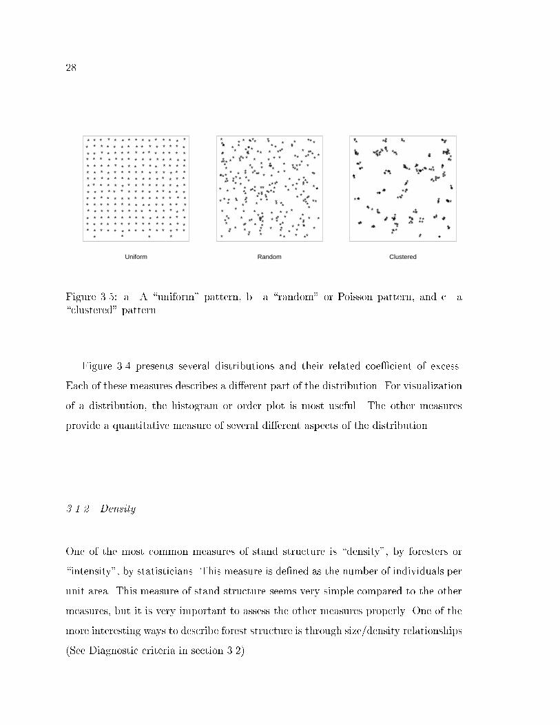
Figure 3.5: a. A \uniform" pattern, b. a \random" or Poisson pattern, and c. a\clustered" pattern

Figure 3.4 presents several distributions and their related coe�cient of excess.

Each of these measures describes a di�erent part of the distribution. For visualization

of a distribution, the histogram or order plot is most useful. The other measures

provide a quantitative measure of several di�erent aspects of the distribution.

3.1.2 Density

One of the most common measures of stand structure is \density", by foresters or

\intensity", by statisticians. This measure is de�ned as the number of individuals per

unit area. This measure of stand structure seems very simple compared to the other

measures, but it is very important to assess the other measures properly. One of the

more interesting ways to describe forest structure is through size/density relationships

(See Diagnostic criteria in section 3.2).

29

Table 3.1: Table of values for spatial patterns for the three example plot shown abovein Figure 3.5.

Statistic Uniform Random Clustered

Number 229 250 236

Skellam-Moore 175.01 85.48 18.59

Clark & Evans 1.74 1.01 0.41

Brown 0.99 0.51 0.34

Pielou 0.63 1.09 2.81

Hopkins' F 0.26 1.02 11.36

Hopkins' N 0.19 0.53 0.85

Holgate F 0.08 0.11 0.30

Holgate N 0.37 0.39 0.62

3.1.3 Spatial pattern

The spatial pattern in a forest stand has been viewed as a two-dimensional point

process. Given a pattern of points in two-dimensions, one question that statisticians

have asked is whether the pattern is randomly distributed or not. Point patterns

can assume a range of patterns from \uniform", to \random", to \clustered" (Ripley,

1981; Diggle, 1983) (Figure 3.5.). If a pattern represents tree locations in a forest,

a \random" pattern is called a Poisson forest, as the points are Poisson distributed.

Many tests for nonrandomness have been developed for just such questions. In most

of the following tests, they determine if the pattern is Poisson distributed. First, a

number of �rst order tests will be examined. Table 3.1 lists the values for the above

tests for the three patterns in Figure 3.5. The speci�c of how to calculate each index

can be found in Appendix A.

� Skellam-Moore

30

Both Skellam (1952) and Moore (1954) developed an approach to look at mapped

point patterns at a time when average quadrate samples were common. Their

main question is the validity of randomness of pattern assumption for the

quadrate samples? Skellam-Moore is a test that for the Poisson assumption

is �22m. It was noted by Pielou (1959) noted that estimates of intensity (n=A)

are poor using distance methods and that independent estimate of intensity

from quadrates should be used .

� Clark and Evans

Clark and Evans (1954) were attempting to develop a general index of spatial

pattern. They noted that the assumption of random spatial plant distribution

is not valid of observed plant patterns. Their method was a test of randomness

for populations of known density and they state the measure uses only the

nearest neighbor, it ignores the majority of the spatial relationships to other

plants. With the index of aggregation, if the spatial pattern is random, R = 1;

clustered, R! 0; and uniform, R! some arbitrary upper limit.

� Brown

The Brown index of aggregation is the geometric mean of squared distances over

the arithmetic mean and is independent of area. The index G ranges from 0 to

1 with G! 0 for \clustered" pattern and G! 1 for \uniform" pattern (Brown

and Rothery, 1978).

� Hopkins'

The Hopkins' index of aggregation is the ratio of the distance from a randomly

chosen point to its nearest neighbor tree and the distance from that nearest

neighbor tree to its nearest neighbor.

31

HopF =

mXi=1

d2(p�ti)i

mXi=1

d2(t�ti)i

; (3.6)

where d(p�ti)i is the distance from a random point to it's nearest neighbor in-

dividual i and d(t�ti)i is the distance from individual i to it's nearest neighbor

individual. This test has an F distribution with F (2m; 2m) (Hopkins, 1954).

Byth and Ripley (1980) presented a standardized index based on this test as:

HopN =1

m

mXi=1

24 d2(p�ti)i(d2(p�ti)i + d2(t�ti)i)

35 ; (3.7)

This index has a Normal null distribution, N(12; 112m). As HopN ! 0, it indi-

cates a more \uniform" pattern; and as HopN ! 1, it indicates a more \clus-

tered" pattern.

� Holgate

The Holgate index is based on the ratio of the distance from a random point

to its nearest neighbor and the distance from the same random point to the

next nearest neighbor (Holgate, 1964). The Holgate indices have the same null

distributions as the Hopkins' indices.

� Pielou

Pielou (1954) noted the value of the di�erence between tree to tree distances,

point to tree distances, and intensity estimates as separate properties of a spatial

pattern. The bias is introduced by using the same sample for estimating density

is discussed above.

32

Pielou (1959) de�nes an index of nonrandomness that has the following range �

is 1 if for a \random" pattern, �! 0 for \uniform" patterns and �! arbitrary

upper limit for \clustered" patterns.

Demonstrates the relative range of value for three very di�erent patterns. The

Hopkins' N index will be used in this paper because it is scaled between 0 and 1, the

index seems to be the most well behaved in extreme conditions, and it is relatively

easy to calculate.

The spatial indices discussed so far are all �rst order (i.e. measures use the distance

to the nearest neighbor. The Holgate index does incorporate distance to the second

nearest neighbor but does not exploit higher order information. There are a set of

statistics that exploit more of the information by evaluating the relationship of a set of

points to all other individuals. A few such statistics are Ripley's K, and semi-variance.

� Ripley's K

This second-order test looks at the relationship of each point to all other points

(Ripley, 1981; Diggle, 1983; Tomppo, 1986). If the point pattern is Poisson, the

cumulative distribution of a number of individuals within a given distance will

follow �t2, where t is the maximum distance observed.

This statistic provides more information about the underlying process than the

previously mentioned statistics. If K(t) > �t2 the process is \clustered" and if

K(t) < �t2 the process is \uniform." Additionally, the size and range of the

deviations from �t2 can be determined about the process.

� Semi-variance

Semi-variance is the basis for many geostatistic tools and is a di�erence between

all points a given distance apart. (Palmer, 1988). This concept may be applied

in one, two, or more dimensions; here the two dimensional case is discussed.

33

This statistic must be applied to a value that can be measured as a continuous

variable across the study area. This technique has potential for resource vari-

ables such as nitrogen N or water content of the soil as well as aggregated stand

variables at landscape scales. Palmer (1988) plots several hypothetical process

patterns and the resultant semivariogram as well as several scales of plant data.

While these measures provide more information about the underlying spatial pat-

tern the calculation time and the added value of the information may not be worth

the added computation time required.

3.1.4 Species

The relative number of individuals in each of species has also been used as a measure of

the structure of plant communities. In the pollenology literature the relative amounts

of the various species is the main descriptor of forest structure (Von Post, 1946; Henry

and Swan, 1974; Whitmore, 1982; Winkler, 1985; Brubaker, 1986; Liu, 1990; Ford,

1990). Additionally, models have been built to predict the change in the species

composition of a plant communities (Botkin et al., 1972a; Botkin et al., 1972b; Urban,

1990). As with the size distributions, species can be described with distributions;

however, the species are categorical and do not have an inherent order. Methods of

ordering species by tolerance, abundance, or serial stage have been used.

3.1.5 History

Forests develop as a set of distribuance, regeneration, and mortality events interacting

with the above elements of stand structure. When discussing history; however, the

logic may become circuitous, because di�erent histories can interact with similar

patterns or distributions or species and produce very di�erent stand structures. This

is not to say the processes are not predictable; but if one ignores the history of a

forest, the assumptions about the stand development may be in error.

34

A number of studies have demonstrated through stand reconstruction how the

history of a stand interacts with the pattern, size distribution, and species to create

the current forest structure (Oliver and Stephens, 1977; Oliver et al., 1985; Oliver

and Larson, 1990).

3.2 Diagnostic criteria

Silviculturists have developed many relationships that help assess the condition of a

stand and its potential for treatment. The relationships are called diagnostic criteria

(Oliver, 1992) and are a familiar way of examining a stand for many silviculturists.

Model builders can utilize this experience by building growth models that present the

results of forest simulations in these familiar ways.

Diagnostic criteria can be grouped into three categories, each with a speci�c di-

agnostic use. The categories include stocking or stand density measures, growth or

change measures, and condition or vigor measures.

3.2.1 Stocking and stand density

Stocking and stand density are two related concepts which sometimes are confused

as the same thing, stocking refers to the relative density of a given stand compared

to some standard stand. Usually, the standard is a \normal" stand but the concept

of normality is not widely use today. Stand density is some average stand measure

per unit area (Bickford, 1957; West, 1983).

Spacing in relation to diameter

Rules of spacing in relation to diameter are often referred to as the \D plus rule of

thumb" and were presented by Matthews (1935). He related spacing, diameter, and

basal area as:

35

S =c � dbhpBA

; (3.8)

where S is the spacing of the stand, c is a constant to correct for the units and �

(Matthews reported a c value of 185 for english units.), dbh is the mean stand diameter

at breast height, and BA is the stand basal area per unit area ( acres or hectares ).

This rule is sometimes used as an aid in thinning a stand to a constant basal area

per unit area. The \D rule" can be plotted over time to indicate the need to thin a

stand.

Density indices

A large number of density measures, formed as indices, include basal area per unit

area, Curtis's relative density (Curtis, 1971), crown competition factor (Krajicek

et al., 1961), and Drew and Flewelling's maximum line (Drew and Flewelling, 1979).

These are summarized in West (1983), including their formulas and mathematical

relations to each other. All measures provide ways to scale a stand's density from

zero to a species' \maximum." Each measure emphasizes a di�erent component of

stand density and therefore explains a slightly di�erent part of the story.

Spacing in relation to height

Spacing|top-height ratios are the ratio of the tree spacing to tree height and have

been applied with the average spacing of the stand and the top-height (i.e. the average

height of some arbitrary number of the largest trees in the stand). These measures are

argued to be better than diameter-based measures of stocking since height is reported

to be less a�ected by stand density. Wilson (1946) reported the following relationship

of spacing to height

TPA =A

(b � ht)2 ; (3.9)

36

where TPA is the trees per unit area, A is the square units per unit area (e.g square

feet per acre or square meters per hectare), b is a fraction of height and ht is the top

height for the stand. Wilson advocated thinning stands to a given value of b. This

measure can be applied as the average spacing of a tree with its competitors and its

height to provide an index of an individual tree's growing space and an idea of the

range of density conditions within the stand.

Spacing in relation to volume

Drew and Flewelling's (1979) maximum size-density line provides an example of

this type of relationship. The advantage of volume is that it integrates diameter

and height into a single measure; however, it has the disadvantage of being tied to

a speci�c volume equation. An interesting variation is the relation of bole area to

number of trees (Lexen, 1943). Bole area provides a measure more closely related to

stem respiration. With sapwood taper equation now available (Maguire and Hann,

1987), sapwood volume relationships may prove of interest.

Density Management Diagrams

All of the above relationships can be plotted in log-log space to produce density

management diagrams. Density management diagrams are plots of trees per unit

area (e.g. trees per acre or trees per hectare) versus average size (e.g. mean diameter,

mean height, mean volume). The movement of a stand through this space provides

information about a stand's relative position in terms of a hypothetical maximum size-

density relationship and the rate at which the stand is approaching that maximum.

These relationships were �rst described by Reineke (1933) in which the average

of some size component of the stand (e.g.. diameter (Reineke, 1933; Long et al.,

1988; McCarter and Long, 1986), height (Wilson, 1951), or volume (Drew and

Flewelling, 1979)) is plotted against the average number of stems per unit area. These

are probably the most developed of the diagnostic criteria, with the largest body

37

of literature, including two growth models based entirely on assumed trajectories

through this space (Smith and Hann, 1984; Lloyd and Harms, 1986). These plots

present the mean trend of the the size variable, but provide no information about the

character of the underlying distribution.

3.2.2 Growth or change

Growth or change is probably the measure of most interest to silviculturists managing

a forest stand. Because growth or change is the means by which a stand moves from

the current condition to another, presumably more desirable, condition.

Diameter Growth

Diameter is the most accessible of the tree dimensions because it is easy to measure.

Diameter at breast height has no particular biological signi�cance. Many people

have advocated measuring diameters at proportions of tree height (e.g. 10 percent

of tree height), however, this may not be logistically convenient. Diameter growth

is the easiest of the tree's dimensional changes to remeasure. With paint a semi-

permanent mark can be placed on the stem for diameter remeasurement. Additionally,

increment cores can easily be collected to determine radial increment. These growth

measurements can be plotted over time to determine rate of diameter change.

Years per unit measure (e.g., years per inch or years per centimeter) is a measure of

the diameter growth rate of an individual tree. By analyzing the trends in individual

tree diameter growth rate, one can assess how well the tree has been competing in the

past and whether the rate will increase or decrease. The diameter growth can also be

plotted in cumulative form, presenting diameter over time. This plotting can be easily

done in the �eld by marking, radial increment versus time on graph paper. When

observing diameter growth a decline is expected as a consequence of the geometry of

placing the new wood around an ever increasing core. This must be accounted for in

any interpretation of diameter growth.

38

Height Growth

Height is one of the most di�cult dimensions of a tree to measure because the view

of the tree tops become obscured as stands grow taller. Height is one of the more

biologically signi�cant dimensions, since it is directly related to a tree's competitive

status. Height growth is usually determined in two ways: One is repeat measurement

of individual tree heights. This method often yields poor estimates of height growth

except when the trees are short. Large variances are usually observed, even when the

same person remeasures the heights. The second method is to measurement of height

growth from stem analysis. This is usually the preferred method; however, the tree

is destroyed in the process.

Volume Growth

Traditionally, volume growth is the feature of a stand that most interest foresters.

Volume is a variable that is an estimate as opposed to variable that is actually mea-

sured. Stem volume is the feature of a stand that is most closely related to timber

products. Under a timber management objective, stand volume growth can be a mis-

leading statistic in that stand volume growth can be added to stems that will make

useful products or to stems that can not be harvested. A stand of tree with less total

volume but on a fewer stem will usually be more valuable.

3.2.3 Condition or vigor

The third set of diagnostic criteria focus on the condition or vigor of a stand and

how that stand might respond to a thinning. These include measures such as height-

diameter ratio, leaf area index, crown closure, and sway period.

39

Height-Diameter Ratios

Height-diameter ratios are the ratio of a tree's height to it's diameter in the same

units. This tool can be used to track the stability of a stand of trees over time and

providing a indication of the time when the stand will become unthinnable (Wilson,

1946; Wilson, 1951). Traditionally, silviculturists have considered trees with height-

diameter ratios greater than 100 as unstable for thinning.

Leaf area index

Leaf area index is a standardized measure of the amount of leaf surface area per unit of

ground surface area. Leaf area index can be a very useful indicator of a stand's ability

to respond to thinning and/or fertilization (Vose and Allen, 1988). The problem with

leaf area index is that to date there is no reliable, easy method of measurement.

Currently the most common technique is to predict leaf area from the tree's diameter

or sapwood basal area and species. Another technique is to measure the relative light

interception of the canopy and use these values to estimate leaf area index. These

techniques are highly variable; and a reliable, fast e�cient method is needed to allow

the widespread use of this index.

Live crown ratio

Live crown ratio is a estimate of the amount of crown on a individual tree. It can

be used in determining the vigor of a tree. This is a measure that is used widely by

growth models and some volume equations (Walters, 1986; Valenti and Cao, 1986)

Crown Closure

Crown closure is an estimate of the proportion of sky covered by foliage observed from

beneath the canopy. This measure can be estimated from spherical densiometers in the

�eld or from hemispherical photographs in the o�ce. Crown closure is an imprecise

40

estimate of the amount of leaves in a stand. This is not as useful as LAI because

it only indicates the presents or absences of leafs with little information about the

number if present. It is, however, useful for determining site utilization.

Sway period

Sway period is a measure of the periodicity of the sway of a tree. This is a biome-

chanical property of a tree. The theoretical period can be calculated as

T = k �M � L3 (3.10)

where T is the period of sway, k a constant of proportionality, M is the mass of a

weight on the beam at height L. This relation was reported by Sugden (1962) as a

method of crown classi�cation for determination of stand competition. Sugden sug-

gested using this method to determine the amount of foliage weight on a tree. Others

have questioned the biological reason for tree stem form and have used mechanical

support arguments to explain tree form (Wilson and Archer, 1979; McMahon and

Kronauer, 1976).

3.3 Stand dynamics and growth models for management

Silviculturists use growth models to predict stand change and how disturbances will

e�ect that change. Silviculturists usually describe stands in terms of stand structure

using the elements of the spatial arrangement, the relative sizes, species, and density

in intuitive, if not quantitative, terms. How these elements change over time provides

the other important element of stand structure | history.

All models are designed to provide a speci�c type of answer. If a model is used

for a purpose other that the one that it was originally designed for the user should

reexamine the all the assumptions and relationship built into the model and access

the consequences of those assumption on the current problem.

41

3.3.1 Related models

Related models have had an in uence on the approach to silvicultural modeling de-

scribed in this paper. These three models have taken approaches that are quite

di�erent than that of the majority of forest growth models. The �rst is the TASS

model (Mitchell, 1975), second a stand dynamics demonstration model CROGRO

(Fellows, Sprague and Baskerville, 1983) designed to teach the principles of crown

development to students, and the third is the many publications of models for the the

management of Scots pine (Pukkala, 1987; Pukkala and T. Kolstr�om, 1987; Pukkala,

1988; Pukkala, 1989a; Pukkala, 1989b; Pukkala, 1990).

The TASS model

The Tree And Stand Simulator (TASS) is a distance dependent, forest growth model

that uses a three-dimensional description of a part of the stand to simulate tree

growth and crown interaction. Th amount of foliage on a given tree determines the

trees height growth and in turn branch growth. The resultant stem increment is

allocated over the stem. A description of the functions in the TASS model are as

follows.

This model has been calibrated to a larger amount of permanent sample plot

(PSP) data for Douglas-�r (Pseudotsuga menziesii (Mirb.) Franco ) and versions

are being prepared for western hemlock (Tsuga heterophylla (Raf.) Sarg.) and sitka

spruce (Picea sitchensis (Bong.) Carr. ). The exibility of the TASS approach is

that many treatment e�ects can be simulated for pure stand of calibrated species

(Mitchell, 1975). The TASS models have been used to generate managed stand yield

tables for British Columbia (Mitchell and Cameron, 1985). The ability to mix species

currently has been envisioned but not implemented. Many of the equations of this

model can be found in Appendix B.

42

Crown Length

Maximum Crown Length

Height

Maximum Branch Length

Foliage volume

Figure 3.6. Diagram of the crown description for the TASS model

The CROGRO model

While this growth model had much less e�ort expended in its construction it is no

less interesting in concept. The CROGRO model was built as a tool to teach crown

development to students (Fellows et al., 1983). The approach made a number of

assumptions about crown interactions. It was calibrated with regional growth and

yield information and was evaluated by presentation to students, foresters, and aca-

demics. One of the most interesting features is that the model results are displayed

in two-dimensional computer drawing of the trees and their crowns.

Height growth is the driving function of this model. The actual height growth

is determined by reducing the potential height growth by the ratio of the projected

vertical cross-sectional area of the crown to the optimal vertical cross-sectional area

of the crown. The equations for this model can be found in Appendix B.

The driving functions are based on local yield curves. The estimate of growth

is modi�ed by the vertical projection of crown area and this is modi�ed by tree

43

Maximum Branch Length

Branch Base and TipHeight difference between Branch Angle

Maximum Crown Radius

Figure 3.7. Diagram of the crown description for the CROGRO model

interaction. Figure 3.8 illustrates the basic parameters of crown shape in this model.

The functions are rate curves derived from the weibull function �t to the height-age

curve.

This approach was found acceptable for the design purpose. The dynamics of

open grown crowns were not well represented; however the essential dynamics of

stand grown trees were acceptably represented.

Pukkala's Model

Pukkala has build a spatial growth model called MikroMikko for Scots pine (Pinus

sylestris L.) in Finland. Average stand characteristics were used to generate a tree list

44

for a spatial pattern. In Pukkala (1989b), two methods were presented for generating

diameters from a spatial pattern. The �rst method assumed that trees with many

close neighbors will be small and trees with few close neighbors will be large. The

second method used the local spatial pattern to predict a diameter distribution and

then this distribution is sampled to determine the diameter for the subject tree. Then

the spatial pattern and the predicted diameter were used to predict tree height. The

equation for diameter and height can be found in Appendix B.

Pukkala's model used these relationships in the following sequence.

1. Stand average statistics such as density and total stand basal area are speci�ed

for the stand;

2. The tree coordinates are generated as a realization of a suitable spatial process;

3. The diameters are predicted from the spatial pattern;

4. The heights are then predicted as a function of the spatial pattern and the

diameter.

The output of these models are displayed in two and three-dimensional displays

showing also statically predicted crown dimensions. This model has been extensively

tested against non-spatial models built from the same data. Pukkala (1987) has

shown that the non-spatial models may be considerably in error, if a stand has large

amounts of variability.

Pukkala's has put these models to interesting uses. In one study, Pukkala explored

the e�ects of roads for thinning equipment placed through a stand at 20 meter intervals

(Pukkala, 1989b). If the remainder of the stand was thinned uniformly, the model

predicted that the trees along the thinning road would have higher growth than the

internal trees within the strip. By experimenting with these simulations he devised a

45

n

i = 1

i

4

3

2

1 Θ

Θ

ΘΘ

θΣ

5 meters

Figure 3.8: Diagram of the spatial competition measure in Pukkala's (1987) growthmodel.

46

thinning proportion between the skid roads that equalized growth among all trees in

the residual stand.

Another model presented by Pukkala (1987), along with work currently in progress

Pukkala (Personal communication, 1990), explored the spatial relationship of an over-

story canopy and the initiation and survival of tree seedlings.

Chapter 4

METHODS

\Seek simplicity, and distrust it"

Alfred North Whitehead

\... our position is that modeling is an art; that the �rst task is to de�ne

objectives; the second to select a consistent view of the system; and only

later, and if appropriate, to use a mathematical description."

Mike West and Je� Harrison, 1989. Bayesian Forecasting and Dynamic

Models

Stand management for a variety of objectives is di�cult when the di�erent ob-

jectives are expressed in diverse measures (e.g., numbers of roosting pairs of birds,

board foot volume for timber, acre-feet of water yield for drainage basins. Stand

structure can be the common language among the various disciplines that deal with

stands (Oliver, 1992). Foresters can produce forests that will meet the multi-resource

goals, if the range of stand structures and the timing of those structures can be de-

scribed for the diverse objectives. Management with the stand structure approach

requires a through knowledge of stand development and how management can e�ect

that development.

Adaptive models of stand dynamics are based on the idea that theories of forest

stand dynamics can be used to de�ne the relationships for projection of stand struc-

tures. These general relationships can then be calibrated to given stand conditions

to \localize" the predictions. Adaptive models of stand dynamics are less precise at

48

estimating volume, although they can accurately describe stand structure and the

change in that structure over time.

Adaptive models of forest growth can be built in many forms. An individual tree

model of stand dynamics will be presented in the current example. The individual tree

model assumes that each tree responds to its immediate environment. In individual

tree models, it is easier to describe the expected biological relationships, to de�ne the

e�ect of disturbances, and to re ect species di�erences. There are disadvantages to

the individual tree approach as well. Individual tree models have more parameters to

de�ne, which makes the models more di�cult to test. A whole stand model has the

advantage of being easier to parameterize and test data, faster to run, and if stand

average estimates are all that is needed they may provide the information needed.

When designing any type of model, there are facts that e�ect the performance of

the model whether admitted or not. These facts are especially important to consider

in the design process:

� Models are nothing more than an explicit statement of a person's or group of

people's ideas about a system;

� All models are biased by the modeler in the parts they choose to include and

exclude;

� A modeling approach's success depends on attempts by several modelers the

determine overall feasibility of the approach.

4.1 Use of an adaptive stand dynamics model

An adaptive stand dynamics model is designed to utilize whatever data is collected

from the stand of interest and information on the species' age-height trends. This

procedure allows the general tree and stand dynamics trends to be adjusted to the

49

local site and species speci�c conditions or to expected growth patterns. The following

are the steps need to set up the model:

� Data gathered from the stand or group of stands of interest are used to parame-

terize the functions in the model. This tree list should include species, diameters

at breast height, total tree height, height to crown base, average crown width,

and a stem map of the trees. Obviously this information is not always avail-

able or obtainable. The stem map is use to calculate an Hopkins' index. An

alternative method would be to measure a number of distances between random

points and the nearest neighbor tree (e.g. 30 distances) and then from those

same thirty trees to their nearest neighbor tree. If the stand is mapped and

the random sample points determined in the parameterization, it is less likely

to be biased. Crown measurements are very important in this type of model to

de�ne the parameters properly, since the growth of a given tree is a function

of crown size. Only general theoretical trends are built into the model|no re-

gional trends. This means that the results are very dependent on the data that

the user collects. The advantage of this design is the exibility; however, this

places more responsibility on the model user. Flexibility means the ability to

adjust the growth trends within the model to re ect the expect growth patterns

for the stand and species.

� The height growth trends must also be de�ned for each species considered. Two

approaches can be taken to obtaining this information. The �rst is to take

data from stem analyses of trees representing dominant or co-dominant growth

patterns for the various species. This is rather labor intensive and needs to be

done when the results are likely to di�er from existing age-height curves. The

other approach is to use existing regional age-height curves for the species and

site.

50

Value Cell - End result of current model.

Decision Cell - input information is used to decide on course of action.

Deterministic Cell - item will always produce the same output for the same input.

Probablistic Cell - item measured with error or a random number.

Figure 4.1. The de�nitions for the shapes in an in uence diagram.

These data and information are used by a parameterization routines to determine

the various parameters estimates for the model. The data and information described

here are the variables needed to parameterize the model presented in the example. If

the functions were changed to have other variables, the data and information require-

ments would change.

Using these parameter estimates, projections are made for the stand; then, alter-

native management scenarios can be considered. The topic of selection of management

scenarios using this growth model will be left for future work.

4.2 Components of an adaptive stand dynamics model

Figure 4.1 presents the de�nitions for the four basic shapes used in in uence diagrams

(Shachter, 1986). These diagrams are acyclic (i.e. loops are not allowed in in uence

51

diagrams). If a decision box is entered with only one outlet, the previous procedure

is continued until the exit condition is obtained. Another description method is

mathematical notation where the pertinent variables will be describe at the time of

presentation. Then each model is described verbally.

4.2.1 Component models for stand generation

The �rst set of submodels generate a simulated stand from input parameters. The

models have components for the prediction of spatial pattern, static height pattern,

crown size, and diameters of the trees. A simulation approach is used to make the

stands grow, for two reasons. First, the growth models are a combination of determin-

istic and probabilistic techniques. The deterministic part describes the mean trend

for the relationship, the probabilistic part adds variation similar to that observed in

the input data. This type of model is designed to capture the general behavior of

the stand structure, not to accurately predict a speci�c tree. Second, the proposed

approach is to explore a di�erent technique. The aim is to describe the stand dy-

namics behavior of the speci�c stand, not precise yield estimates of a speci�c stand.

The emphasis in on de�ning a range of outcomes. Figure 4.2. illustrates the order in

which the submodels are executed.

4.2.2 Generation Process

Spatial pattern

The process of generating a suitable spatial pattern has problems associated with it.

Several people have developed methods to generate spatial patterns. The problem

is that one speci�c resultant spatial pattern can be generated by several possible

generating processes; therefore, simply knowing the spatial pattern does not provide

information about underlying generating processes. The approach used in this study

is to group patterns into two types, stands started as plantations and stands started as

52

Tree List

Foliage

Diameter Crown SizeHeight

Species

SpatialPattern

Figure 4.2. The in uence diagram for the generation process

ParametersSpatial

Process

PatternTest Pattern

Lattice

ProcessNeyman-Scott

ProcessDetermine

Origin of Stand

Figure 4.3. The in uence diagram for the pattern generation process.

natural regeneration. This distinction that should be rather easily made by foresters.

Once classi�ed, two di�erent generating processes are used. These two processes

use similar parameters but make di�erent basic assumptions about the underlying

pattern. The process of calculating the appropriate parameters involves an iterative

routine in which starting parameters are chosen. A simulated stand is generated and

compared to the input pattern. To make this comparison, a statistic must be used.

The statistic chosen for this study is Hopkins' N , it is easy to interpret, it is

53

11

11

1

11

11 1

1 1 11

11 1

1 1 1

2

2

2

22

22 2 2

2 2 2 22

22

22 2

2

3

3

3

3

33

33 3

3 3 33 3 3

3 3 33

3

44

44

4

44

4

4 44 4 4

4 4 4 4 44 4

55

55

55

5

55

55

55 5

55

5 5 5 5

(A) Lattice

Amount of Distance Variation

Hop

kin’

s N

5 10 15 20

0.0

0.2

0.4

0.6

0.8

1.0

11

1

1 1 1 1 1 1 1 11 1 1

1 11

11 1

2

2

22

2 22

22 2 2 2 2

2 2 22

22 2

33

3

3

33

33 3

33 3 3

3 3 33

3 33

44

44 4

44

44 4

4 4 4

4 4 44 4

4

4

55

55

5 5

5

5 55 5

5 5 55 5 5

5 55

(B) Neyman-Scott

Amount of Distance Variation

Hop

kin’

s N

5 10 15 20

0.0

0.2

0.4

0.6

0.8

1.0

Figure 4.4: The range of Hopkins' N for various pattern generation parameters. The(A) lattice process and the (B) Neyman-Scott process. These diagrams illustratethe e�ect of varying the input parameters to the two generating processes and theresultant hopkins indices generated as a outcome.

rather easy to calculate so can be calculated at each step of the iteration process, and

it provides reasonably stable results. A diagram of the submodel is in Figure 4.3.

If a plantation origin is selected, a lattice process is used to generate the spatial

pattern. The lattice process assumes the trees are arranged on a lattice pattern with

variation from that pattern. The nominal spacing is determined from the density of

trees and the area of the sample plot. A grid of points is establish with a random

starting point. These points are called the \parent points" and are the intended

location of the trees. From each parent point a random azimuth and distance within

a speci�ed range are chosen to establish the location of the child point. Trees are

assigned to children points only. The parameters for a lattice process are the spacing

of the parent points, the variation range for each child point and the number of child

points. In plantations the number of child points is usually one. Additionally all

points are tested to be within the range of the simulated plot. This process seems

54

to work well for Hopkins' values from 0 to 0.5 as seen in Figure 4.4(A). The main

method of changing the Hopkins' value of the simulated stand is by changing the

variation range parameter.

If a natural stand origin is selected, a Neyman-Scott process is used. Neyman and

Scott (1972) were astronomers, who developed this process to generate patterns for

simulated galactic clusters. The generating process is based on a random or Poisson

point pattern. The random or Poisson pattern is generated by a binomial distribution

of two uniform random numbers for the required number of parent points. From these

parent points, a random azimuth and random distance, within a range limit, is applied

to produce each child point. Additionally, all points are tested for the range of the

simulated plot. This process works well for Hopkins' values from 0.5 to 1.0 as seen

in Figure 4.4(B). The parameters to match the Hopkins' index can be determined

by changing the variation range and the number of child points associated with one

parent point. Figure 4.4 is a graph of how the parameters can be varied to generate

di�erent spatial patterns.

Species

The next step in the tree list generation process is to assign species to each point in

the generated pattern. The parameters for this submodel are the relative proportion

of each species on the sample plot. From these proportions, each point is randomly

assigned a species in the same overall proportion as the original sample plot. The

assumption is that the number of of individuals of a given species in the simulated

stand will be in the same proportion as in the current stand. This is probably only

valid if the age of the generated stand is near the age of the observed stand. A better

approach would be to grow a stand from a assumed regeneration event; however, the

number of assumptions and time to calculate this approach would make the result a

dubious improvement. Figure 4.5 presents the in uence diagram for this submodel.

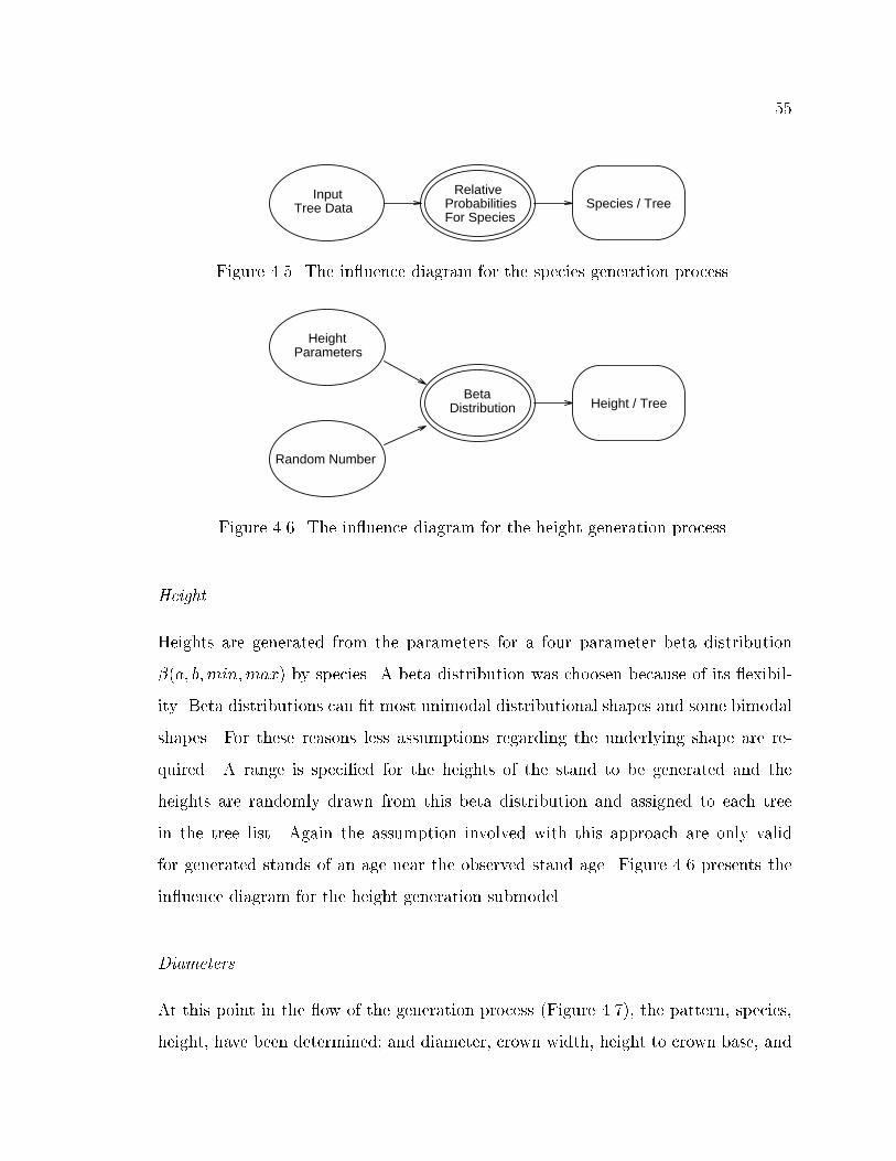
55

Tree DataInput

For Species

RelativeSpecies / TreeProbabilities

Figure 4.5. The in uence diagram for the species generation process.

Height / TreeDistributionBeta

Random Number

ParametersHeight

Figure 4.6. The in uence diagram for the height generation process.

Height

Heights are generated from the parameters for a four parameter beta distribution

�(a; b;min;max) by species. A beta distribution was choosen because of its exibil-

ity. Beta distributions can �t most unimodal distributional shapes and some bimodal

shapes. For these reasons less assumptions regarding the underlying shape are re-

quired. A range is speci�ed for the heights of the stand to be generated and the

heights are randomly drawn from this beta distribution and assigned to each tree

in the tree list. Again the assumption involved with this approach are only valid

for generated stands of an age near the observed stand age. Figure 4.6 presents the

in uence diagram for the height generation submodel.

Diameters

At this point in the ow of the generation process (Figure 4.7), the pattern, species,

height, have been determined; and diameter, crown width, height to crown base, and

56

Height

Dbh / TreeDiametersCalculate

Tree

ParametersDiameter

Random Number

Figure 4.7. The in uence diagram for the diameter generation process.

amount of foliage are left to be determined.

For the generation process, diameters are predicted as a direct relationship to

height. A height/diameter equation is parameterized for the input data and is used

in the inverted form to predict diameter. This done to allow the �tting of a linearized

form to the input diameter-height data.

di =

"ln(hti � bht)� b0

b1

# 1

b2

; (4.1)

where di is the diameter at breast height for the ith tree in the tree list, hti is the

height of the ith tree in the tree list and bht is the breast height for the measurement

system (i.e. english or metric). This equation is applied with random error determined

from the input data to mimic relationships found in the original data. The residual

from the above �t diameter-height equation are estimated as a beta distribution. A

random draw from this distribution is added to the deterministic prediction from the

above equation. The resultant diameter-height values mimic the original distribution

of the input data.

57

Height to

Height toCrown Base

Crown Base

Equation

Tree

Crown Width

Heights

Height/DiameterHeight/DiameterTree

Parameters

Calculate

Crown Width

Crown Base

Random Number

Parameters

Figure 4.8. The in uence diagram for the crown generation process.

Crown size

Crown size for the generation process is predicted from diameter using the following

equation. The inverse of this relationship has been used for years in aerial photogram-

metry as a method of determining volumes for sample plots on aerial photographs

(Paine and McCadden, 1988). The relationship is of the form:

cwi = b0 + b1db2i ; (4.2)

where di is the diameter for the ith tree, cwi is the crown width for the ith tree in

the tree list, and the b's are the regression coe�cients.

Crown length is determined as a deterministic ratio to crown width for the species.

Again a better method to determine that crown widths and crown lengths is to grow

the stand from an inital state. But the generation process is designed to produce a

simulated stand of a similar character to the input stand.

Figure 4.8 is the in uence diagram for the height to crown base prediction in the

generation submodel.

58

Foliage

The foliage calculation function has three basic components for determination of

foliage amount per tree. These three parts are the calculation of the surface area

of a geometric solid of the dimensions of the tree crown, the conversion of the surface

area of the solid to foliage area, and the calculation of the variation in these functions.

They are diagrammed in Figure 4.9.

The idea of calculating foliage amount from the surface area of a solid is from

Maguire (1989). In this paper, Maguire discusses the relationships of gross crown

dimensions to to sapwood area at crown base. Sapwood area at crown base has been

shown to be a good estimator of leaf area in Douglas-�r (Grier and Waring, 1974;

Waring et al., 1982; Whitehead et al., 1984; Espinosa Bancalari et al., 1987) and in

other species (Rogers and Hinckley, 1979; Dean and Long, 1986; Keane and Weetman,

1987).

The �rst part is to calculate the surface area of a geometric solid. The solid can

be any shape from a paraboloid, to a cone, to a neiloid. The di�erences between the

various areas are negligible compared to the variation added, so the formula for the

lateral surface area of a cone was used.

The conversion factor allows the assumption that foliage amount is related to

surface area in some proportion. A conversion factor of one is assumed in the current

example. As better methods of measuring canopy foliage are developed, this type of

factor will become important in distinguishing between foliage conditions.

An amount of variation was added to the predictions to indicate the assumed

uncertainty of the relationship. A variation of �20% of the surface area was added as

a random normal to the foliage amount in the current example. The other equations

can be found in Appendix C.

SA � N(dSA; :2 �dSA); (4.3)

59

Parameters

FoliageFoliage / Tree

Foliage areaSurface area to

Proportion

Calculate

DistributionBeta Error

Surface AreaCalculate

VariationProportion

TreeCrown Length

TreeCrown Width

Random Number

Foliage

Figure 4.9. The in uence diagram for the foliage generation process.

60

Upon completion of the generation process, a tree list has been created that has

a similar statistical character as the originally sampled stand. This generated stand

is used as input to the growth submodel of the model.

4.2.3 Component models for growth

The growth submodel is the portion of the model that changes the list of tree variables

from a given time to the next time step. An in uence diagram of the relationship

of the components is given in Figure 4.10. From the diagram it will be noted that

the process is much less dependent on the calculations in the other submodels at the

current time step. The process is very dependent on the values in the starting time

tree list.

The philosophy of the growth submodel is based on the idea that the rate of change

of an individual tree on a given site is dependent on that tree's height and crown size.

Three factors in uence the rate of change of a tree: the maximum potential rate of

change for the species on the site, the ability of the tree to produce photosynthate (a

function of the size of the crown), and limits on the size of the tree (analogous to the

respirative cost for increasing size). This model uses these simple concepts about the

change of trees and aggregates the trees into stands. This section will now examine

the strengths and weaknesses of the approach.

Height Growth

Height growth is one of the more complex functions within the submodel. It is

designed to use readily available data assuming an interpretation of that data, to

predict height growth of a tree. Figure 4.11 is the in uence diagram for the height

growth submodel.

The height growth submodel has three parts; a rate �, a modifying function to

determine the role of relative foliage amount, and a modifying function to determine

the role of relative tree size in height growth. The rate value � is the periodic rate

61

Tree ListEnding

FoliageCalculate

Regeneration

Diameter Growth

Crown Change

Height Growth

Tree ListStarting

Figure 4.10: The in uence diagram for the growth process. Note that only the crownchange part depends on the values of other parts. All parts depend on the startingconditions.

DerivativeWeibull

Parameter

HeightCalculate

Exponential

Parameter

HeightEnding

Height Growth

Function

Function

Height GrowthSize

Height GrowthFoliage

Tree ListStarting

Figure 4.11. The in uence diagram for the height growth process.

62

Height growth and Height growth rate

Time (yr)

Hei

ght g

row

th (

m)

0 50 100 150

0.0

0.2

0.4

0.6

Time

010

2030

40H

eigh

t (m

)Figure 4.12: Example height-age curve with the base curve (solid line) and the �rstderivative of the curve, which is the height growth rate curve (dotted line).

of growth at the in ection point of a height-age curve for the species and site. This

represents the period in a tree's life for which it is growing at the fastest rate. This

point is determined by �nding the maximum of the �rst derivative of the height-age

function. This point is used as the maximum growth rate (Figure 4.12).

The �rst modifying function predicts the e�ect of foliage amounts other than the

amount of foliage on a tree growing at the maximum rate. First, a tree with a full

crown (crown length equal to tree height) of the size of the maximum rate fol� is

assumed to grow at the maximum rate �. Further, additional foliage is not assumed

to increase the tree's height growth rate. Trees with less foliage than the maximum

63

Foliage Ratio

Mod

ifer

0.0 0.2 0.4 0.6 0.8 1.0

0.0

0.2

0.4

0.6

0.8

1.0

Height Ratio

Mod

ifer

1.0 2.0 3.0 4.0 5.0

0.0

0.2

0.4

0.6

0.8

1.0

Figure 4.13: Example foliage ratio and height ratio functions for the height growthsubmodel

rate amount fol� will grow as a full crowned tree of that crown length. The main

e�ect of this part of the equation is to reduce growth on trees with foliage amounts

less than the maximum rate amount fol�. Figure 4.13a is a graph of the shape of the

multiplicative e�ect of this part of the equation.

The second modifying function de�nes the e�ect of trees growing larger or the

upper asymptote of the height/age curve. This part of the equation assumes that

height growth rate will slow down as trees become larger relative to the size of a

tree at the maximum rate size h�. This part of the submodel de�nes the asymptotic

behavior of the resultant height-age curve. The equation for this submodel is of the

form:

�h = �

"fol

fol�

#a1266664hmax

0BBBB@0@ h

h�� age�b

1Ac

c

0BBBB@exp

��

h

h��age�

b

�c!hh�� age�

1CCCCA1CCCCA =�

377775 ; (4.4)

where �h is the change in a tree's height, � is the rate at the in ection point of the

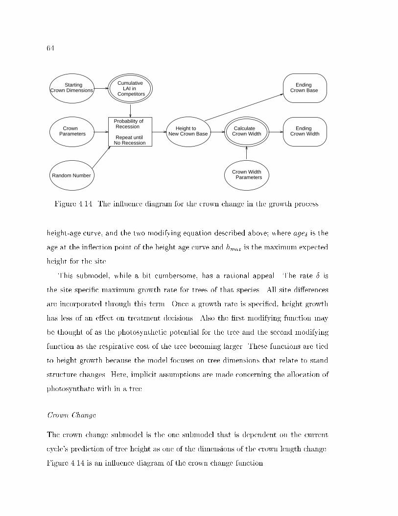
64

Ending

EndingCrown Dimensions

Starting

ParametersCrown Width

Crown WidthCalculate

Crown Width

Crown Base

New Crown BaseHeight to

No RecessionRepeat until

RecessionProbability of

CompetitorsLAI in

Cumulative

Random Number

ParametersCrown

Figure 4.14. The in uence diagram for the crown change in the growth process.

height-age curve, and the two modifying equation described above; where age� is the

age at the in ection point of the height-age curve and hmax is the maximum expected

height for the site.

This submodel, while a bit cumbersome, has a rational appeal. The rate � is

the site speci�c maximum growth rate for trees of that species. All site di�erences

are incorporated through this term. Once a growth rate is speci�ed, height growth

has less of an e�ect on treatment decisions. Also the �rst modifying function may

be thought of as the photosynthetic potential for the tree and the second modifying

function as the respirative cost of the tree becoming larger. These functions are tied

to height growth because the model focuses on tree dimensions that relate to stand

structure changes. Here, implicit assumptions are made concerning the allocation of

photosynthate with in a tree.

Crown Change

The crown change submodel is the one submodel that is dependent on the current

cycle's prediction of tree height as one of the dimensions of the crown length change.

Figure 4.14 is an in uence diagram of the crown change function.

65

Competitor

Subject Tree

Non-Competitor

θ

θ

Figure 4.15. Illustration of determination of competitor trees.

A vertical pro�le of the leaf area index of all trees considered competitors of

the subject tree is determined by summing the proportional amounts of each tree's

vertical foliage pro�le into a cumulative vertical pro�le. The equations to accomplish

this summations are as follows:

Lk =mXj=1

GroundXk=Canopy Top

�jA�(aj; bj) Ij;k; (4.5)

where Lk is the cumulative leaf area index of competitors for each tree at level k from

the top of the canopy, m is the number of trees considered to be competitors to the

subject tree, � is the amount of leaf area on tree j, and A is the area associated with

the maximum distance of the m competitors to each subject tree. Beta probability

density functions (p.d.f.) �() with parameters aj and bj are for the species of com-

petitor tree j and are used to distribute the amount of leaf area � along the crown

length of competitor tree j. Ij;k indicates whether level k is within the crown length

of competitor tree j.

66

Leaf Area IndexCumulative

Height

Competitors

Competitors

Subject Tree

Non-Competitor

θ

θ

θθ

θ

Figure 4.16: The method of determining the cumulative leaf area index in competitors

For all competitor trees, a cumulative leaf area index pro�le from the top of the

canopy is constructed (Figure 4.15). A probabilistic prediction is based on the current

leaf area competition at the crown base for the crown base changing one height unit

(e.g., 0.3 meters in the current example). The process is stopped for that subject tree

for that cycle if the equation predicts no change. If the equation predicts a crown

change then the process is repeated until no change is predicted, and the latest crown

base value becomes the crown base in the new tree list.

Given this cumulative leaf area pro�le the probability of the crown recession of

one height unit is determined by:

P (i; k) = 0:5 +1

�arctan [�(Lk � LAI)] ; (4.6)

where P (i; k) is the probability of the crown receding at height k to height k+1 on tree

i, which is predicted by an arc tangent function (Figure 4.17). The LAI determines

67

the location of the in ection point on the \x" axis. This LAI is the level of leaf area

index in competitors at which the foliage on the subject tree dies.

Regeneration

Seedling regeneration is predicted from a distribution describing the number of seedlings

per time step for a given species. A random variate is drawn from this distribution

for the number of seedlings to consider for regeneration for the time step. A cumu-

lative leaf area index pro�le is calculated for the seedling location, just as for the

crown change function, and probability of survival is predicted for the seedling. If the

seedling survives, it is added to the tree list as a live tree. Figure 4.18 is an in uence

diagram of the regeneration process.

Mortality

Tree mortality is usually one of the weakest links in forest growth models. Trees

can die for many reasons or from many causes. In general, trees die from suppression

through competition, windthrow, breakage, and attack by insects or disease. Pest- and

disease-caused mortality are host- and site-speci�c and require special submodels of

those species. Breakage and windthrow are functions of the soils, species, combination

of the physical dimensions of the tree, and local wind environment.

Suppression is relatively the easiest to predict and is a function of reduced growth

from competition with neighboring trees. It is the only mortality form predicted in

this model. There is no explicit mortality function in the current version of the growth

model. A tree dies when a tree's crown recedes above tree height. This calculation

only represents one form of suppression mortality.

68

Leaf area index in competitors above point of consideration

Pro

babi

lity

P(i,

k)

0 2 4 6 8 10

0.0

0.2

0.4

0.6

0.8

1.0

Figure 4.17: A plot of an example arc tangent function for predicting crown recession,� = 4 for this example

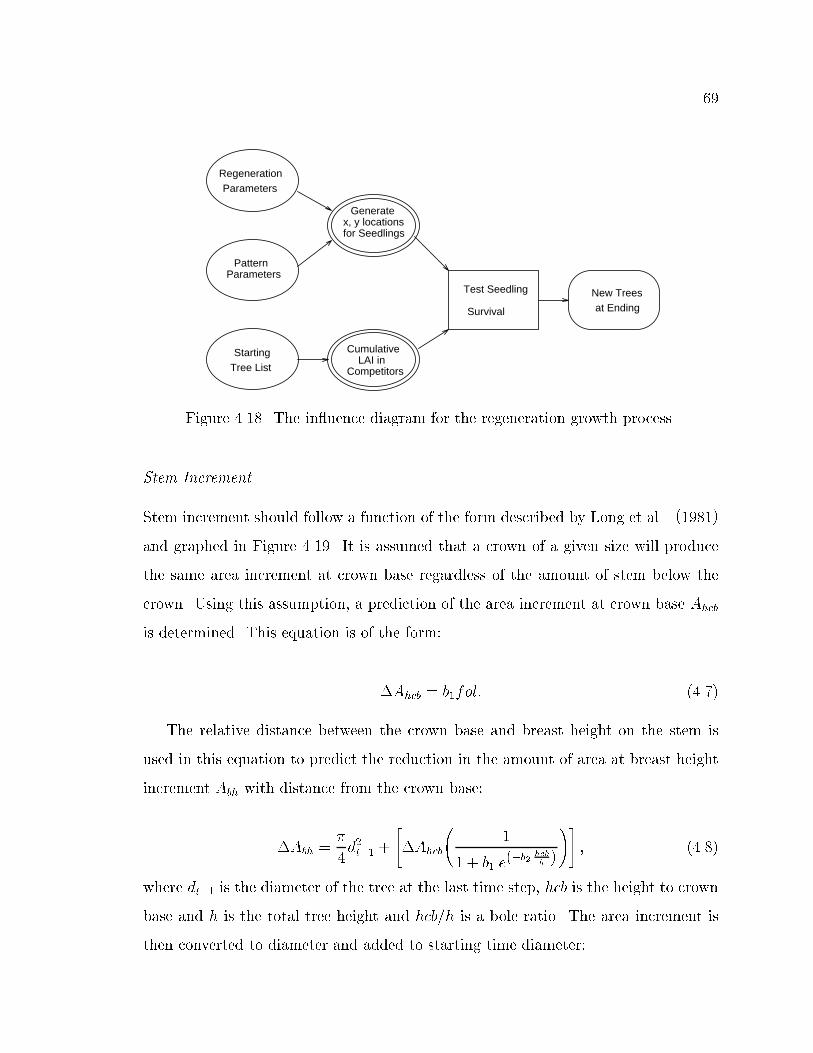
69

at EndingNew Trees

Survival

Test Seedling

for Seedlingsx, y locations

Generate

CompetitorsLAI in

Cumulative

ParametersPattern

ParametersRegeneration

Tree ListStarting

Figure 4.18. The in uence diagram for the regeneration growth process.

Stem Increment

Stem increment should follow a function of the form described by Long et al. (1981)

and graphed in Figure 4.19. It is assumed that a crown of a given size will produce

the same area increment at crown base regardless of the amount of stem below the

crown. Using this assumption, a prediction of the area increment at crown base Ahcb

is determined. This equation is of the form:

�Ahcb = b1fol: (4.7)

The relative distance between the crown base and breast height on the stem is

used in this equation to predict the reduction in the amount of area at breast height

increment Abh with distance from the crown base:

�Abh =�

4d2t�1 +

"�Ahcb

1

1 + b1 e(�b2 hcb

h )

!#; (4.8)

where dt�1 is the diameter of the tree at the last time step, hcb is the height to crown

base and h is the total tree height and hcb=h is a bole ratio. The area increment is

then converted to diameter and added to starting time diameter:

70

Relative Area IncrementRelative Area Increment

HeightHeightRelativeRelative

Crown base

Crown base

Figure 4.19: The assumed shape of the stem area increment, similar to functionsdescribed by Long et al. (1981).

dt = 2

s�Adbh

�+ dt�1; (4.9)

Stem increment calculated with this approach re ects the changing size of the

crown.

4.2.4 Assumption of the Current Approach

There are many assumptions that a�ect the behavior and results of an adaptive stand

dynamics model. Here the assumptions are stated to clarify both thinking about the

model and expectations of the output.

� Stand responses are the aggregate of an individual tree's response to its imme-

diate environment.

71

DiameterEnding

Dbh Area

Crown BaseArea At Calculate

FunctionLogistic

Tree ListStarting

ParametersDiameter

Figure 4.20. The in uence diagram for the diameter growth process.

� Tree height increment is a function of crown size and tree size and the potential

growth rate for a species on a speci�c site.

� Crown size, as the productive part of a plant, is the dominant force changing a

tree's size.

� Stem area increment at crown base is a function of crown size regardless of the

tree size.

� Stem increment at other points on the stem fellow a function similar to Long et

al. (1981) (Figure 4.19).

� Leaf area is related in some proportion to the surface area of a geometric solid

representing a crown shape of that species (Maguire and Hann, 1987).

These assumptions are used to guide construction of model components.

4.3 Presentation of Model Output

An often overlooked part of growth models is type of output. Output should convey

useful information and be exible enough so the user can request information in a

desired form. Many forest growth models are built by modelers who, by virtue of

their interest and training, are most interested in the numerical output; however,

72

users relate more to graphical displays of the same information. Many people can

grasp graphical displayed relationships much quicker than tabular output. A growth

models that presents output in many imagitive ways could bring the results of grwoth

models to many more people.

Over the years, silviculturists have developed many relationships that help access

the condition of a stand and the potential for treatment of that stand. The relation-

ships are called diagnostic criteria (Oliver and Larson, 1990) and are familiar ways of

examining a stand for many silviculturists. Once a person is accustomed to analyzing

stands using these tools, a background of experience arises that aids the manager

in using of the tools. Model builders can utilize this experience by building growth

models that present the results of forest simulations in these terms.

4.4 Example System

\I cannot really imagine any other law of thought than that our pictures

should be clearly and unambiguously imaginable."

L. Boltzmann 1897

4.4.1 Objective

This chapter presents the detail of an adaptive stand dynamics model. There are many

ways to implement these ideas, some that work better than others. This dissertation

presents the ideas with the intent of conveying the concepts, rather than the details

of a particular implementation.

4.4.2 Design

This model is designed to use a \Run and Display" approach as opposed to a \Display

as you Run" approach. The growth submodel is \Run," and output is stored in an

output �le or data structure. Then, a separate display part of the model will read

73

that �le or data structure. This approach has several advantages. Any time step

in the growth sequence can be easily viewed; plots over time are easily made; and,

when many batch runs are needed this task is much easier. In \Display as You

Run" approach, the program plots the current values of the projected tree list. The

run usually must be reinitiated and rerun to show previous states of the stand; and

over-time plots are not available until the end of the run.

This model uses a simulation approach; input tree data are distilled into a set of

parameters that describe a stand. A simulated stand is then generated from these

parameter sets and used as the initial condition for model runs. Because of the

stochastic nature of the models, the output will di�er with each run with identical

input. If averages are desired, several runs must be averaged to obtain estimates of

the predicted mean and range.

4.4.3 Components of the models

The \GENERATE" program is a set of routines that produces a tree list from a

parameter set. As stated in chapter 4 the program steps through the routine in the

following order.

The function to generate the random numbers used in the C routines is the \ran3"

function from Numerical Recipes (Press et al., 1988), and inside S the \runif" function

is used.

Pattern { The �rst step is to generate a spatial pattern for the simulated stand.

One of two generating processes is used. If the stand is natural in origin then a

Neyman-Scott process is used; otherwise a lattice processe is used.

� Neyman-Scott process generates a pattern of random \parent points" which

are invisible and used as the origins for a cluster of \children points". The

algorithm is given a number of \children" and a maximum variation dis-

tance. For each \child point" a random azimuth and random distance is

74

used to determine the location of the `child point." This process is used

for Hopkins' indices between 0.5 and 1.0.

� Lattice process generates a nominally spaced grid of points with a random

start as the \parent points". These are used as the origin for the \children

points". Again the algorithm is given a number of \children" and the

maximum variation distance. Random azimuth and distance is determine

to locate the child point. The lattice process is used to generate patterns

with Hopkins' indices between 0.0 and 0.5.

Species { The species subroutine generates a species for each point in the previously

generated pattern. This is done randomly based on the relative proportion of

the species found in the original input data set.

Height { The initial heights are generated as random variates from a beta distri-

bution, with the parameter estimated from the input data. The range of the

generated data can be changed to allow for the generation of stands that di�er

in size from the input data.

Diameters { The diameters are generated using height/diameter equations inverted

to predict diameters from heights. An error component is added that mimics

the error in the original input data.

Crown Width { The crown width equations are exponential functions which use the

diameters to predict crown widths. An error component is added re ecting the

errors within the original data.

Crown Base { The height to crown base is a deterministic ratio between the width

and the length of the crown.

75

Foliage { The amount of foliage is determined as a ratio of the crown surface area to

foliage area. This ratio is currently assumed to be one, but in the near future

could be measured.

The \GROW" program takes a generated tree list or a previously grown tree list

and a set of tree parameters to grow the tree list through one or more time steps.

The program can start at any existing year in the list and project the list from that

time forward.

Height growth { The height growth subroutine predicts the change in height which

is added to the height at the previous time. The height change is a function of

the crown size and tree size at the previous time.

Crown change { The crown change subroutine �rst builds a cumulative leaf area pro-

�le of all competitors for each subject tree. From this information, a prediction

of the probability of the crown base receding is made; and the crown recedes if

a random uniform number drawn is greater than the probability. If the crown

recedes the process is iterated until the crown does not recede.

Diameter growth { The diameter growth of a tree is predicted as a function of the

crown size. For example, if the trees crown increases, diameter growth increases.

The area increment at the crown base is �rst predicted; then, the ratio between

the area increment at crown base and the area increment at breast height is

determined. The area increment at breast height is then converted into diameter

increment and added to the previous diameter.

Regeneration { The amount of regeneration is determined �rst by randomly drawing

a number of potential seedlings to test per unit area for the next time step. Each

seedling is assigned a coordinate, and the competition around that coordinate is

76

determined. The seedling is established and added to the tree list with a small

random height if the competition is less than the establishment threshold.

Mortality { Mortality is not explicitly modeled but mortality is determined by the

trees inability to grow because of loss of crown.

Utilities are a set of subroutines used to manipulate the tree list to simulate

stand treatments. These include thinning and pruning. The potential for a fertilizer

subroutine exists but is not implemented in the current work.

Thinning { This subroutine simply identi�es trees pointed to on a tree map and

removes them.

Prune { This subroutine removes the lower part of tree crowns in either variable or

�xed lifts.

The set parameter routines are used to take an input tree list and build the

parameters needed to run the model. These routines can be used with many types

of data or information. The parameters are in two major groups: the plot level

parameters and the species-speci�c tree level parameters. Plot level parameters relate

to the density or intensity, spatial pattern, species mix, type of measurement units

and time step length. Tree level parameters describe distributions of tree variables in

the original input data, growth rates of the input growth data, and assumed crown

recession parameters.

Hopkins { The Hopkins' index of non-randomness is used to determine the spatial

pattern of input data. This index was chosen because of the relative ease of

calculation and the logical range for ease of interpretation. The Hopkins' index

is determined for the input data and is used as a target for the generated spatial

patterns.

77

Set plot parameters { This routine queries the user for the general plot level param-

eters of the original input stand. It also queries for labeling and measurement

unit information.

Set species parameters { This routine steps the user through the setting of species

speci�c parameters. Parameters can set through assumptions while others are

�t to input data when ever possible. First, diameter/height equations are �t to

the input data for use by the generating functions. The relative abundance of

various species are noted; the height distribution and the distribution of errors

for each equation are estimated, with the beta distribution function using the

moments method. Next, the crown routine is called and the user is asked to

set a crown shape and width parameter visually for the species. Figure 5.1 is

an example of the visual screen that can be changed interactively. The height

growth routine is called next. It is a rather involved routine and is explained in

the next section. Then, a crown width relationship is �t to the input data for

use in stand generation. Finally, parameters that cannot be determined from

the input data are added with reasonable values to complete the parameter set.

This routine must be repeated for each species in the stand.

Set height growth parameters { The height growth functions are one of the key

functions within the model. The function �rst reads the input height/age data

for the species. These data can be from published height/age curves, stem

analysis data, or repeat measurement data from permanent plots. A guided

�tting technique is used because these data do not always extend over the

range of the time for which predictions will be made. The routine requires as

input height/age pairs and a target asymptote value. A exible cumulative

Weibull model is plotted with starting values �t to the data. The user can

vary the parameters until the �t \looks good". When the technique was tried,

statistically �t models worked well when complete or near complete data were

78

Distance (ft)

Hei

ght (

ft)

0 20 40 60

020

4060 Shape = 0.8

Crown Width = 0.66

Crown Length = 42

Figure 4.21: Example of the set crown parameter display. The user can interactivelyset the three parameters.

79

11

1

1

1

1

1

1

11

1

22

2

2

2

2

2

2

2

2

2

3

3

3 3

3

3

3

3

3

33

4

4

4

4

4

4

4

4

4

4

4

5

5

5

5

5

5

5

55

55

6

6

6

6

6

6

6

6

6

66

7

7

7

7

7

7

7

7

7

77

8

8

8

8

8

8

8

8

88

8

9

9

9

9

9

9

9

9

9

99

Height - Age

0 50 100 150

010

2030

40

Tree age (yr)

Hei

ght (

m)

Figure 4.22: Example of the set height parameter display. The number line are theheight age trajectories for nine trees and the solid line is the equation �t to thesedata.

available but were hard to guide to the desired asymptote when complete data

are not available.

Once the age/height curve is determined, its �rst derivative with respect to

height is calculated and the maximum found (see Figure 4.12). This maximum

is the potential height growth rate for the species on the given site. The data are

now divided at this maximum point and functions �t to the parts using a guided

technique. This technique allows use of surrogate variables to substitute for the

original age axis. This surrogate substitution is accomplished by expressing the

age as a ratio to the maximum rate age. The foliage ratio and size ratio are

then expressed within the same range.

80

Feet

0 20 40 60 80 100

020

4060

8010

0

Fee

t*

*

*

*

*

*

*

*

*

*

*

*

*

*

*

*

*

*

*

*

*

*

**

*

*

*

*

*

*

*

*

**

*

*

***

*

*

*

*

*

*

*

*

* *

*

*

*

*

*

**

*

*

*

*

*

*

*

*

*

*

**

*

*

*

*

*

*

*

*

*

*

*

*

*

*

*

*

*

*

**

*

*

*

*

**

*

*

*

*

*

*

*

*

*

*

*

*

*

*

*

*

*

*

*

*

*

*

*

*

*

*

**

*

*

*

**

*

*

*

*

*

*

**

*

*

*

*

*

*

*

*

*

*

*

*

*

*

*

*

*

*

*

*

*

*

*

*

*

*

*

*

* **

*

*

*

*

*

*

*

*

*

*

*

*

**

*

**

*

*

*

* *

*

* **

*

*

*

*

*

*

*

*

*

*

*

**

*

*

*

*

*

*

*

*

*

**

**

*

**

**

*

*

*

*

*

*

*

* **

*

* *

*

*

*

* *

*

*

*

*

*

*

*

*

*

*

*

*

*

*

*

*

*

*

*

*

*

*

*

*

*

*

*

*

*

*

*

*

*

*

*

*

*

*

*

*

*

*

**

*

*

*

*

*

*

*

**

*

*

*

*

*

*

*

*

*

*

*

*

*

*

*

*

*

*

*

*

**

*

*

*

*

*

* *

*

*

*

*

*

*

*

*

*

*

*

*

*

*

*

*

**

*

*

*

*

*

*

*

*

*

*

*

*

*

*

*

*

*

*

*

*

*

*

*

*

*

*

*

*

*

*

*

*

*

**

*

*

*

*

*

**

*

*

*

*

*

***

*

Stand Map of Hugo Peak Stand at age 45

Figure 4.23: Example stand map from the growth model. The circle represent thecrown diameters.

Display is a set of routines used to display the output of a growth model run.

Some routines have been constructed to date; but, as stated earlier, others can be

constructed as well. The display scale units are in either English units (inches and

feet) or metric units (centimeters and meters).

Map { The map routine plots the x, y coordinates of each tree stem at a given time

and represents the diameter of the crown with a circle. This is in map view, or

from above the stand. Figure 5.3 is a sample output of this routine.

Identify map items { This routine allows the interactive identi�cation of trees within

the map. When using X-windows the user can point to trees and click. The

81

Distance (ft)

Hei

ght (

ft)

-20 0 20 40 60 80 100 120

020

4060

8010

0

Stand Profile of Hugo Peak Stand at age 45

Figure 4.24. Example stand pro�le from the growth model.

tree number will appear near the tree. The numbers of all trees are printed if

the routine is run with other graphics interfaces.

Pro�le { Pro�le is a routine that will present a side or pro�le view of the stand from

either the x or y side and over any speci�ed range. Trees are plotted using a

tree outline de�ned in the set crown routine. Figure 5.4 is an example of the

stand pro�le plot.

Pro�les over time { This routine allows the user to view an individual tree over the

entire growth run. This view is useful to observe the history of height growth

and crown change visually. Figures 5.5 and 5.6 are examples of the pro�le over

time routine.

82

Hugo Peak Stand - Tree 188

Time (5 yr)

Hei

ght (

ft)

020

4060

8010

012

0

1 2 3 4 5 6 7 8 9 10 11 12

Hugo Peak Stand - Tree 117

Time (5 yr)

Hei

ght (

ft)

020

4060

8010

012

0

1 2 3 4 5 6 7 8 9 10 11 12

Figure 4.25. Example individual tree pro�les from the growth model.

83

Hugo Peak Stand - Tree 107

Time (5 yr)

Hei

ght (

ft)

020

4060

8010

012

0

1 2 3 4 5 6 7 8 9 10 11 12

Figure 4.26. Example individual tree pro�le from the growth model.

Plot variables { This routine simply plots any variable in the tree list against any

other variable in the tree list. The routines allows the user the look at relation-

ships between variables such diameter and height. Figure 5.7 is an example of

the variable plotting function.

Plot variable over time { This routine produces a time trace for each tree of the

variable requested. Figure 5.8 is an example plot over time.

Histogram variables { This routine plots a histogram of the speci�ed variable at the

speci�ed time. Figure 5.9 is an example of the histogram.

Plot leaf competition { This routine displays the cumulative leaf area index pro�le

used to predict crown recession and the current tree pro�le. If a user steps

through the time steps or tree numbers, they can see how the crown of an

individual tree interacts with the leaf area of the competitors. Figure 5.10 is an

84

*

**

*

**

* *

*

*

**

* *

**

*

*

* *

*

*

* *

*

*

*

*

*

*

*

*

*

*

*

**

**

*

*

*

**

*

*

*

*

*

*

*

*

*

*

*

**

*

*

*

*

*

*

*

*

*

*

*

*

*

* *

*

*

*

*

*

*

*

*

*

*

*

*

**

**

*

*

*

*

*

*

**

**

*

*

*

*

*

*

**

*

*

*

*

*

* *

*

*

*

*

*

*

*

**

*

*

*

*

*

*

*

*

**

*

**

*

*

**

*

*

*

*

*

**

*

*

*

*

*

*

*

* *

*

*

*

*

*

*

*

*

*

*

*

*

*

*

*

*

*

*

*

*

*

*

*

*

*

*

*

*

*

*

*

*

*

**

*

*

**

*

*

**

*

*

*

*

*

*

*

*

*

*

*

*

**

*

* *

*

*

*

*

**

*

*

*

*

*

*

*

*

*

*

*

*

**

*

**

**

***

*

*

**

*

*

**

*

*

**

*

*

*

**

*

*

*

*

*

*

*

*

**

*

*

*

*

*

*

*

*

*

*

*

*

*

*

*

*

*

*

**

*

*

*

*

*

*

*

*

*

*

*

**

*

*

*

*

*

*

*

*

*

*

*

*

*

*

*

*

*

*

*

*

*

*

*

*

*

*

*

*

*

**

* *

*

*

*

** **

*

*

**

*

**

* *

*

*

*

*

*

*

*

*

*

*

**

*

*

*

*

*

*

**

*

*

*

*

*

*

*

*

*

*

*

**

*

*

*

*

*

**

*

*

*

*

*

*

**

*

*

*

**

*

*

*

*

*

*

**

*

Diameter at breast height (in)

Hei

ght (

ft)

0 2 4 6 8 10 12

020

4060

80

Hugo Peak Stand 28 - Diameter vs. Height

Figure 4.27. Example plot of diameter versus height.

85

Time (5 yr)

Hei

ght (

ft)

2 4 6 8 10 12

020

4060

8010

0

Hugo Peak Stand - Height vs. Time

Figure 4.28. Example plot of individual tree heights over time.

86

20 40 60 80

05

1015

20

Height (ft)

Num

ber

Hugo Peak Stand 28 - Height

Figure 4.29. Example histogram of heights.

87

Cumulative LAI in competitors (sq ft)

Hei

ght (

ft)

0.0 0.5 1.0 1.5

010

2030

4050

Distance (ft)

Hei

ght (

ft)

-5 0 5 10

010

2030

4050

LAI profile of tree 386 year 1

Figure 4.30: Example cumulative leaf area index pro�le. The x axis on the left plotis the cumulative leaf area index (LAI). The x axis on the right plot is distance.

example of the plot of leaf area competition.

Plot variable rank order { This routine displays an ordered plot of the trees in a

stand versus a variable. The order variable need not be the plotted variable.

As described earlier, this plot is one way of looking at stand structure. Figure

5.11 is an example of ordered plots of variables.

Density management space { The density management relation is a common tool

used by foresters to evaluate the condition of a stand and the change within the

stand. This routine allows the plotting the relation of trees per unit area and

the quadratic mean diameter of the stand. Maximum lines are species speci�c

and so are not routinely plotted; however, a line of speci�ed stand density index

88

Relative Rank

Hei

ght (

ft)

0.0 0.2 0.4 0.6 0.8 1.0

020

4060

Hugo Peak Stand 28 - Height ordered by height

Figure 4.31. Example plot of rank order of the heights.

89

*

**

**

**

*****

********

Trees per acre

Qua

drat

ic M

ean

Dia

met

er

1 10 100 1000

15

1050

100

Hugo Peak Stand 28 - Density Management Diagram

Figure 4.32: Example size{density plot over time. The point represent the locationof the stand a successive points in time. The solid line is an assumed maximum forDouglas-�r of SDI 595.

can be overlayed to provide a reference point as done in Figure 5.12. Figure

5.12 is the track of a stand of Douglas-�r (Pseudotsuga menziesii) and the stand

density index (SDI) 595 (The assumed maximum for that species (Drew and

Flewelling, 1979)) for reference. Points indicate locations of the stand at each

�ve year time step.

Structure plots { A set of multi-plots allow many plots to be viewed at various times.

These include change in a set of reverse ordered tree heights with time, the

change in spatial index over time, change in species mix over time, and change in

the height distribution over time. In Figure 5.13 a few of the largest tree at time

90

one remain the largest tree though out the model run. Figure 5.14 illustrates

a large range in the density of the stand; however, the spatial character as

described by the Hopkins' index does not change. Figure 5.15 illustrates the

relationship among the three species in the stand. In this particular run only one

species Douglas-�r (df) survived to the end of the run. Figure 5.16 illustrates

the height distributions for the stand.

Tree means { This is a non-graphical routine to report the means and variances for

all the tree list variables.

One feature of the current model is the method of conveying the output to a user.

The method is based on the assumption that graphical information can be recognized

and comprehended faster than tabular information. There is a three layered approach

to model output display. The �rst level is a \picture" of the stand at the various time

steps. The second level is traditional plot displays such as scatter plots, histograms,

and function plots. Thirdly, the tabulated data are available for question, which arise

from examination of the graphical data.

4.4.4 Description of implementation

This model building e�ort has been an evolution through several computational plat-

forms. Initially the programming was implemented in the C++ programming lan-

guage on a IBM compatible computer. This program worked well in some respects

but, had drawbacks. The �rst problem was to build a graphical interface for the

display of the model output. Using a low level graphics library supplied with the

compiler. Implementation of the program was straight-forward and the concept of

classes the C++ language make the building of the routines relatively fast and easy.

This programming approach was abandoned for three reasons. First, the implementa-

tion grew and the programs became di�cult to debug because of the memory required

by both the debugging software and the program. As the complexity of particular

91

..............................................................................................................................................................................................................................................................................................................................................................................................................................

0100

300

0 20 40

Tim

e 1

.... .. ..... . .... ... .. ... .. ... ..... . .. ....... ... . ... .. .. .. .. ... .. .. ... ..... .. ... ... .. ... ... .......... .... ... ..... .... .... ... ......... . ....... ..... ...... ...... ..... .... .... ..... .. .... .. ... .. ... ... ....... ........ ..................... ....... ......... ....... ... ... ............... ... ... ........ ... ......... .......... ...... ..... ...................... ..... ...... .. ..... ....... ........ .... ........................... .......

0100

3000 20 50

Tim

e 2

.... .. .. ... . .... ... .. ... .. ... .. ... ... ....... ... .... .. .. .. .. ... .. ..... ....... ... ... .. .. . ... .... .. .... .... ... ... .. .... .. .. .. . . ... ..... . .... ... .. ... ... ... ..... .. .... .. .. ... . ...... .. .. . .. ... .. . .. ..... .. ... .. . .. ... ... ... .. .. .. ..... .. ..... ... .. ... .. .... .. ....... .. . .. . ...... ... .. .... ... .... ... . ... ..... .. ... ........ ..... .. .. ... . ..... .... .. ....... ... ... .. .... . ... .. ... .. ...... ........ ....... ........ ............. .........

0100

300

0 20 60

Tim

e 3

.. .. .... .. .. .... ... .. ... ..... .. .. . ... . ... .. . .. .. . .. .... . . ... .. .. .. . .. .... . .... . ... .. .. .... . ... .. .. .. .... .. .. .. .. .. .... .. .. .. .. .... ... .... . ... ... .. .. ... ..... .. .... .. .. ... . . .. ... .. .. . .. ... .. . .. ..... .. ... .. . .. . .. . .. ... .. .. ....... .. . .... ... .. ... .. .... .. ... ..... .. .. . ...... ..... ... .... .... ... .... .. ... .. ... ... ..... ..... .... ... . ......... .. ....... ... ..... ..... ... .. ..... ...... . ... ... . ........................... ..........

0100

300

0 40

Tim

e 4

.. . . .. .. .... ... . .. . .. .. . ..... .. .. . ... .... ... .. .. . .. ... . .. ... .. .. ... .. .... . ... . . ..... .. .... . ... . ... ...... .. .. .. .. .. . ... .. .. .. .. .... . .. .... . ... ... .. .. ... ..... .. .... .... . .. . . .. ... .. .. . .. ... .. . .. .. ... .. ... .. . .. . .. . .. ... .. .. .. ..... .. . .... ... .. ... .. .... .. ... ..... .. .. . ...... ..... ... ....... . ... .... . . ... .. ... ... ..... ..... .... .... ..... .... .. ....... ... ..... ..... ... .. ... .. .. .... . ... .... .............................. .......

0100

300

0 40 80

Tim

e 5

.. . . ...... .. ... . ... .. .. . ... .. .... . ... .... .. . .. .. . .. ... . . . ... .. .. ... .. .... . ... . . ..... .. . ... . ... . ... . ..... .. .. .. .. .. . ... .. .. .. .. .... . .. .... . ... ... .. .. ... ..... .. .... .. .. . .. . . .. ... .. .. . .. ... .. . .. .. ... .. ... .. . .. . .. . .. ... .. .. .. ..... .. . .... ... .. ... .. .... .. . .. ..... .. .. . ...... ... .. ... ........ ... .... .. ... .. ........... ..... .... .... ..... .... .. ....... ... ..... ..... ... .. ..... ...... . ... .... ........... ................... .......

0100

300

0 40 80

Tim

e 6

.. . . ...... .. .... .. . .. .. . .. . .. .. .. . ... .... .. . .. .. . .. ... . . . ... .. .. ... .. .. .. . ... . . .... ... . ... . ... . ... . ..... .. .. .. .. .. . ... .. .. .. .. .... . .. .... . ... ... .. .. ... ..... .. .... .... . .. . . .. ... .. .. . .. ... ... .. .. ... .. ... .. . .. . .. . .. ... .. .. ....... .. . .... ... .. ... .. .... .. . .. ..... .. .. . ...... ..... ... . ... .... ... .... .. ... ... .......... ..... .... ... . ..... .... .. ....... ... ..... ..... ... .. ..... .. ... .. ... .... .............................. .......

0100

300

0 40 80

Tim

e 7

.. . . ...... .. .... .. . .. .. . .. ... .. .. . ... . ... ... .. .. . .. ... . . . ... .. .. ... .. .. .. . ... . . .... ... . ... . ... . ... . ..... .. .. .. .. .. . ... .. .. .. .. .... . .. .... . ... ... .. .. ... .... . .. .... .. .. . .. . . .. ... .. .. . .. ... ... .. .. ... .. ... .. . .. . .. . .. ... .. .. .. ..... .. . .... ... .. ... .. .... .. . .. .... . .. .. . ...... ..... ... ........ ... .... .. ... .. ........... ..... .... ... . ..... .... .. ....... ... ... .. ..... ... .. ... .. ...... . ... ... . ....... ..............................

0100

300

0 40 80

Tim

e 8

.. . .... ... .. .... .. ... ... .. ... .. .. .... . ... ... .. .. . .. ... . . . ... .. .. ... .. .. .. . ... . . .... ... . ... . ... . ... . ..... .. .. .. .. .. . ... .. .. .. .. .... . .. ... . . ... ... .. .. ... ..... .. .... .. .. . .. . . .. ... .. .. . .. ... .. . .. ..... .. ..... . .. . .. . .. ... .. .. ....... .. . .... ... .. ... .. .... .. . .. .... . .. .. . ...... ..... ... ........ ... .... .. ... ... .......... ..... .... ... ......... ... ....... ... ..... ..... ... .. ... .. ....... ... ... . ........... ................... .......

0100

300

0 40 80

Tim

e 9

.. . . .. . ... . . .... .. ... ... .. . .. .... .. .. . ... ... .. .. . .. ... . . . ... .. .. ... .. .. .. . ... . . .... ... . ... . ... . ... . ..... .. .. .. .. .. . ... .. .. .. .. .... . .. .... . ... ... .. .. ... ..... .. .... .. .. . .. . . .. ... .. .. . .. ... ... .. .. ... .. ..... . .. . .. . .. ... .. .. ....... .. . .... ... .. ... .. .... .. . .. ..... .. .. . ...... ..... ... .... .... ... .... .. ... .. ........... ..... .... .... ......... .. ....... ... ..... ..... ... .. ... .. ....... ... .... .....................................

0100

300

0 40 80

Tim

e 10

.. . . .. .. .... . ... .. ... .. . .. . .. . ... .. .. . ... ... .. .. . .. ... . . . ... .. .. ... .. .. .. . ... . . . ... ... . ... . ... . ... . ..... .. .. .. .. .. . ... .. .. .. .. .... . .. ... . . ... ... .. .. ... ..... .. .. .. .. .. . .. . . .. ... .. .. . .. ... ... .. .. ... .. ..... . .. . .. . .. ... .. .. ....... .. . .... ... .. ... .. ... ... . .. ..... .. ... ...... ..... ... ........ ... .... .. ... .. ...... ..... ..... .... ... . ......... .. ....... ... ..... ..... ... .. ... .. ...... . ... .... ... ............ ............... .......

Relative ht

0100

300

0 40 80

Tim

e 11

.. . . .. . ... ... ... .. . .. .. . .. ... . ... .. ... ... ... .. .. . .. ... . . . ... .. .. ... .. .. .. . ... . . . ... ... . ... . ... . ... . ..... .. .. .. .. .. . . .. .. .. .. .. .... . .. .... . ... ... .. .. ... ..... .. .... .. .. . .. . . .. ... .. .. . .. ... ... .. .. ... .. ..... . .. . .. . .. ... .. .. .. ....... ..... ..... ... .. .... .. . .. .... . .. .. . ...... ..... ... ....... . ... .... .. ... .. ...... ..... ..... .... ... . ..... .... .. ....... ... ..... ..... ... .. ... .. ...... . ... .... ....... .... ..........................

0100

300

0 40 80

Tim

e 12

.. . . .. .... .. . ... .. ... .. . .. ... .. .. .. ... ... ... .. .. . .. ... . . . ... .. .. ... .. .. .. . ... . . . ... ... . ... . ... . ... . ..... .. .. .. .. .. . . .. .. .. .. .. .... . .. .... . ... ... .. .. ... ..... .. .... .. .. . .. . . .. ... .. .. . .. ... .. . .. ..... .. ... .. . .. . .. . .. ... .. .. .......... .... ... .. ... .. .... .. . ...... . .. .. . ...... ..... ... ........ ... .... .. ... .. ...... ..... ..... .... ... . ......... .. ....... ... ..... .... . ... .. .......... .. ...... . .............................. .......

0100

300

0 40 80

Tim

e 13

.. . . .. ...... . ... .. ... .. . .. ... . ... ..... ... ... .. .. ... ... . . . ... .. .. ... .. .. .. . ... . . . ... ... . ... . ... . ... . ..... .. .. .. .. .. . . .. .. .. .. .. .... . .. .... . ... ... .. .. ... .... . .. .... .... . .. . . .. ... .. .. . .. ... .. . .. .. ... .. ... .. . .. . .. . .. ... .. .. .. ..... .. . .... ... .. ... .. ... ... . .. .... . .. .. . ...... ..... ... ........ ... .... .. ... ........ ..... ..... .... .... ........ ... ....... ... ... .. ..... ... .. ... .. .. ..... ... .... ....... .... ................ ..........

0100

300

0 40 100

Tim

e 14

.. . . .. .... .. . ... .. . .. .. . .. ... . ... . .... ... ... .. .. ... ... . . . ... .. .. ... .. .. .. . ... . . . ... ... . ... . ... . ... . ..... .. .. .. .. .. . . .. .. .. .. .. .... . .. .... . ... ... .. .. ... ..... .. .. .. .... . .. . . .. ... .. .. . .. ... ... .. .. ... .. ... .. . .. . .. . .. ... .. .. .. ..... .. . .... ... .. ... .. ... ... . .. .... . .. .. . ...... ..... ... ....... . ... .... .. ... ............. ..... .... .... ..... ...... ....... ... ..... ..... ... .. ..... ..... .. ...... . .....................................

0100

300

0 40 100

Tim

e 15

.. . . .. .... .. . ... .. ... .. . .. ... .... .. ... ... ... .. .. ... ... . . . ... .. .. ... .. .. .. . ... . . . ... ... . ... . ... . ... . ..... .. .. .. .. .. . . .. .. .. .. .. .... . .. .... . ... ... .. .. ... ..... .. .... .. .. . .. . . .. ... .. .. . .. ... ... .. .. ... .. ... .. . .. . .. . .. ... .. .. .. ........ .... ... .. ... .. .... .. . ...... . .. .. . ...... ..... ... . ....... ... .... .. ... .. ........... ..... ....... .......... .. ....... ... ..... ..... ... .. ..... .. ..... ... .... .....................................

0100

300

0 40 100

Tim

e 16

.. .. .. . ... .. . ... .. ... .. . .. ... .. .. .. ... ... ... .. .. ... ... . . . ... .. .. ... .. .. .. . ... . . . ... ... . ... . ... . ... . ..... .. .. .. .. .. . . .. .. .. .. .. .... . .. .... . ... ... .. .. ... ..... .. .... .. .. . .. . . .. ... .. .. . .. ... ... .. .. ... .. ... .. . .. . .. . .. ... .. .. .......... .... ... .. ... .. .... .. . ....... .. .. . ...... ..... ... ........ ... .... . . ... .. ...... ..... ..... .... .... ........... ... .... ... ..... ..... ... .. ..... ..... .. ....... ... ........................... .......

0100

300

0 40 100

Tim

e 17

.. .. .. . ... ... ... .. . .. .. . .. ... .. .. .. ... ... ... .. .. ... ... . . . ... .. .. ... .. .. .. . ... . . . ... ... . ... . ... . ... . ..... .. .. .. .. .. . . .. .. .. .. .. .... . .. .... . ... ... .. .. ... ..... .. .... .. .. . .. . . .. ... .. .. . .. ... .. . .. .. ... .. ..... . .. . .. . .. ... .. .. ....... .. ..... ... .. ... .. .... .. . .. ..... .. ... ...... ..... ... ....... . ... .... .. ... ... .......... ..... ....... .......... .. .......... ... .. ..... ... .. ... .. .. .... . ... .... ........................... ..........

Rank

0100

300

0 40 100

Tim

e 18

.... .. . ...... ... .. ... .. . .. ... .. .. .. ...... ... .. .. ... ... . . . ... .. .. ... .. .. .. . ... . . .... ... . ... . ... . ... . ..... .. .. .. .. .. . . .. .. .. .. .. .... . .. .... . ... ... .. .. ... ..... .. .... .. .. . .. . . .. ... .. .. . .. ... ... .. .. ... .. ..... . .. . .. . .. ... .. .. ....... .. . .... ... .. ... .. ... ... . .. .... . .. .. . ...... ..... .... ....... ... .... .. ... .. ...... ..... ..... .... .... ........... ....... ... ..... .... . ... .. ............ ... .... ............................ .........

0100

300

0 40 100

Tim

e 19

.... .. . ... .. . ... .. ... .. . .. ... .. .. .. ... ... ... .. .. ... ... . . . ... .. .. ... .. .. .. . ... . . .... ... . ... . ... . ... . ..... .. .. .. .. .. . . .. .. .. .. .. .... . .. .... . ... ... .. .. ... ..... .. .. .. .... . .. . . .. ... .. .. . .. ... ... .. ..... .. ..... . .. . .. . .. ... .. .. .. ........ .... ..... ... .. .... .. . ....... .. ... ......... .. ... ........ ... .... .. ... ............. ..... ....... .......... .. ....... ... ..... ..... ... .. ..... ..... .. ....... ....... ..............................

0100

300

0 40 100

Tim

e 20

Figu

re4.33:

Exam

ple

oford

eredheigh

tsplot

overtim

e.Thexaxisisthereverse

ofsize

rank(th

elargest

treeis1)

andtheyaxisistherelative

heigh

tpercen

t(th

elargest

treeis100).

Tree

ranksare

based

ontim

e1;

they

change

order

inthexaxis

with

time.

92

*

*

**

** *

** *

*

**

**

* *

*

*

*

*

*

*

**

**

**

*

*

*

*

*

**

**

*

*

*****

****

**

* *

*

*

*

*

*

**

*

*

*

**

**

*

*

* * **

*

*

* **

**

*

*

**

*

*

**

*

*

**

*

*

**

**

*

**

*

*

*

*

*

*

*

**

**

***

***

*

*

*

*

*

*

* **

**

* *

**

*

*

*

*

**

*

*

**

*

* *

*

*

*

* *

*

**

***

*

*

*

*

*

*

*

*

*

* *

**

* *

*

*

*

**

*

*

*

**

*

*

**

*

*

* *

*

** *

*

*

* *****

*

*

**

** ***

**

***

*

*

*

**

* *

*

*

*

***

**

*

* *

* *

**

**

*

**

* **

*

* *

*

*

*

**

****

*

*

*

*

*

* *

*

* **

*

*** *

*

*

*

*

*

*

**

*

*

*

**

*

**

* **

**

*

* ***

*

*

***

**

*

****

*

**

** ** *

**

*

**

**

**

****

*

**

**

*

*

*

* **

**

*

*

*

*

**

*

*

*

*

*

*

*

* *

*

*

*

*

*

*

*

***

*

**

*

*

* **

*

*

*

**

*

*

***

*

**

* *

**

*

*

**

* *

* *

*

*

*

**

***

*

*

0 40 80

040

80F

eet

Feet

Hopkins = 0.1839014

Time 1

*

*

****

**

**

*

*

*

*

*

*

*

* *

**

*

*****

**

** *

**

*

*

*

**

*

*

*

* *

* **

*

*

*

**

*

*

**

*

**

*

*

*

**

*

*

*

*

*

*

***

* **

* **

*

**

*

*

*

*

*

* *

*

*

*

*

**

*

*

**

*

*

**

*

*

*

*

*

*

*

**

***

*

***

*

* **

**

***

*

*

*

*

***

*

*

*

* *

***

*

***

*

**

***

*

*

*

*

** *

*

*

*

*

**

*

*

*

*

* **

**

* ***

*

**

****

*

***

**

** *

**

***

*

*

*

*

**

*

*

**

*

* *

*

*

*

*

*

*

*

*

*

* **

*

*

*

***

**

*

*

* **

*

* *

* *

*

*

**

**

*

*

0 40 80

040

80

Hopkins = 0.1983205

Time 2

***

***

*

*

*

*

* *

*

****

**

* ****

**

*

*

*

* **

*

**

*

**

**

*

* **

*

*

*

*

**

*

* * *

**

*

*

*

*

*

*

*

*

**

*

*

** *

**

*

*

*

*

*

***

**

**

**

***

*

*

*

***

*

*

*

* *

***

*

**

*

**

* *

*

*

*

*

**

*

*

*

*

**

**

*

*

* ***

*

**

****

*

**

**

****

**

*

**

**

*

**

*

* *

*

*

** *

*

*

* *

*

*

*

**

**

*

**

*

*

*

**

*

0 40 80

040

80

Hopkins = 0.1945829

Time 3

*

***

*

*

* *****

*

****

**

*

* **

*

*

* ** * **

**

**

*

*

**

*

*

**

*

*

**

*

* *

**

*

*

****

**

**

***

*

*

*

**

*

*

*

* *

* *

**

*

**

*

* *

*

**

*

*

*

**

**

*

***

**

***

*

**

**

* **

**

**

*

*

**

***

*

*

* *

*

*

**

*

*

*

* **

0 40 80

040

80

Hopkins = 0.1963809

Time 4

*

*

*

* ***

*

*

****

*

*

* *

*

*

* * * **

**

*

*

*

*

*

**

**

**

**

*

****

**

***

*

*

*

***

* *

*

**

*

** *

*

** *

*

**

**

*

***

***

*

*

**

**

* ***

**

*

*

**

**

*

**

*

*

**

*

**

0 40 80

040

80

Hopkins = 0.2062234

Time 5

*

*

* ***

*

*

****

*

* *

** * **

**

*

*

*

**

**

**

**

*

***

**

***

*

*

*

***

* *

*

**

*

**

*

** *

**

**

*

***

***

** * *

**

*

*

**

**

*

**

*

*

**

**

0 40 80

040

80

Hopkins = 0.1889682

Time 6

*

*

* ***

*

*

****

* *

** * *

**

*

*

*

**

**

**

**

*

*

*

**

***

*

*

***

*

**

*

*

*

** *

**

**

*

***

**

** *

**

*

*

*

***

* *

**

**

0 40 80

040

80

Hopkins = 0.1966938

Time 7

** *

**

*

*

****

*

**

**

*

*

*

**

**

**

**

*

*

*

**

**

*

*

*

*

*

**

*

*

** *

**

**

*

***

**

**

** ***

* *

***

0 40 80

040

80

Hopkins = 0.1935857

Time 8

** *

**

*

*

**

*

*

**

**

*

*

*

**

**

*

**

*

*

*

**

**

*

*

*

* **

*

*

** *

*

**

*

***

**

**

** ** *

***

0 40 80

040

80

Hopkins = 0.1941776

Time 9

** *

*

*

*

**

*

*

**

**

*

*

*

**

**

**

*

*

*

**

**

*

*

*

* **

*

*

** *

**

*

***

**

**

* ** *

**

0 40 80

040

80

Hopkins = 0.1770236

Time 10

** *

*

*

*

**

*

*

**

*

*

*

*

**

**

**

*

*

*

**

**

*

*

* **

*

*

** *

**

*

***

**

*

* ** *

**

0 40 80

040

80

Hopkins = 0.2111597

Time 11

** *

*

*

*

**

*

*

**

*

*

*

*

**

**

**

*

*

*

**

**

*

*

* **

*

*

** *

****

*

**

*

* ** *

**

0 40 80

040

80

Hopkins = 0.1850428

Time 12

**

*

*

**

*

*

**

*

*

*

*

**

**

**

*

*

*

**

**

*

*

* **

*

*

** *

****

*

**

*

* ** *

**

0 40 80

040

80

Hopkins = 0.1952518

Time 13

**

*

*

**

*

*

**

*

*

*

*

**

**

**

*

*

*

**

**

*

*

* **

*

*

** *

****

*

**

*

* ** *

**

0 40 80

040

80

Hopkins = 0.2009852

Time 14

**

*

*

**

*

*

**

*

**

**

**

**

*

*

*

**

**

*

*

* **

*

*

**

****

*

**

*

* ** *

**

0 40 80

040

80Hopkins = 0.1879953

Time 15

**

*

*

**

*

*

**

*

**

**

**

**

*

*

*

**

**

*

*

* **

*

*

**

****

*

**

*

* ** *

**

0 40 80

040

80

Hopkins = 0.1777561

Time 16

**

*

*

**

*

*

**

*

**

**

**

**

*

*

*

**

**

*

*

* **

*

**

****

*

**

*

* ** *

**

0 40 80

040

80

Hopkins = 0.1806601

Time 17

**

*

*

**

*

*

**

*

**

**

**

**

*

*

*

**

**

*

*

* **

*

**

****

*

**

*

** *

**

0 40 80

040

80

Hopkins = 0.1916783

Time 18

**

*

*

**

*

*

**

*

**

**

**

**

*

*

*

**

**

*

*

* **

*

**

****

*

**

*

** *

**

0 40 80

040

80

Hopkins = 0.1994442

Time 19

**

*

*

**

*

*

**

*

**

**

**

**

*

*

*

**

**

*

*

* **

*

**

****

*

**

*

** *

**

0 40 80

040

80

Hopkins = 0.2002466

Time 20

Figure 4.34: Example of spatial pattern plot over time. The Hopkins' index for eachpattern is printed under the map plot.

93

df wh ch

020

0

Time 1

df wh ch

010

020

0

Time 2

df wh ch

050

150

Time 3

df wh ch

040

100

Time 4

df wh ch

040

80

Time 5

df wh ch

040

80

Time 6

df wh ch

040

80

Time 7

df wh ch

020

60

Time 8

df wh ch

020

50

Time 9

df wh ch

020

40

Time 10

df wh ch

020

40

Time 11

df wh ch

020

40

Time 12

df wh ch

020

40

Time 13

df wh ch

020

40

Time 14

df wh ch

020

40

Time 15

df wh ch

020

40

Time 16

df wh ch

020

40

Time 17

df wh ch

020

40

Time 18

df wh ch

020

40

Time 19

df wh ch

020

40

Time 20

Figure 4.35: Example of species barchart plot over time. The x axis are the variousspecies found on the plot and the y axis is the number of individual in each species.

94

0 20 40

020

60

Height (ft)

Num

ber

Time 1

10 30 50

020

Height (ft)

Num

ber

Time 2

10 30 50 70

010

25

Height (ft)

Num

ber

Time 3

10 30 50 70

05

10

Height (ft)

Num

ber

Time 4

20 40 60 80

05

15

Height (ft)

Num

ber

Time 5

20 40 60 80

05

15

Height (ft)

Num

ber

Time 6

40 60 80

05

10

Height (ft)

Num

ber

Time 7

60 70 80 90

05

15

Height (ft)

Num

ber

Time 8

80 90 100

04

8

Height (ft)N

umbe

r

Time 9

85 95 105

04

8

Height (ft)

Num

ber

Time 10

90 100 110

04

812

Height (ft)

Num

ber

Time 11

95 105 115

04

812

Height (ft)

Num

ber

Time 12

100 110 120

05

1015

Height (ft)

Num

ber

Time 13

105 115 125

05

10

Height (ft)

Num

ber

Time 14

110 120 130

04

812

Height (ft)N

umbe

r

Time 15

115 125

04

812

Height (ft)

Num

ber

Time 16

120 130

04

812

Height (ft)

Num

ber

Time 17

125 135

04

812

Height (ft)

Num

ber

Time 18

130 140

04

812

Height (ft)

Num

ber

Time 19

130 140

05

1015

Height (ft)

Num

ber

Time 20

Figure 4.36: Example of histogram of heights plotted over time. The x axis is theheight of the height classes in feet and the y axis is the number of individuals in eachclass.

95

programs increased, the amount of time to debug the program increased exponen-

tially. The size of the programs and the run times on the 386 system became large

and long, respectively. The models were converted to run on a Sun Sparcstation 1.

The DOS software was left at the state of development at the time of the conversion.

The goal is to demonstrate the viability of the approach and not to produce a

commercial product. Additionally, no C++ compilation software was available on the

Sun Sparcstation used. The S statistical package provided all the graphics capability

required and the exibility to implement the model through S user functions, linked

C functions, and stand-alone C programs.

This approach provided a good development environment; for example, a function

or routine that would take a week to code in C or C++ would take about a day in

S. The conversion from C++ version to the S version took approximately a month.

The S version of the model is fragile, requiring a knowledge of S and Unix. One very

nice feature of S is that it is an interactive environment; if the user would like to plot

data in a di�erent way, it is a relatively easy task to write a new function to make

the plot. S is one of several interactive packages that would be suitable for this type

of work. The real advantage is that the package handles the graphics user interface,

allowing the modeler to concentrate on the relationships and behavior of the model.

To implement a system based on graphical displays, a good graphical user interface

is needed. In the current project both interfaces developed from a low level routines

and interfaces developed from high level routine were used. Both system seem to

work well within the limitation of their respective computer. They provide a easy

method to view the output from the growth model and an easy method to visualize

the predictions.

Chapter 5

EXAMPLE SYSTEM

\I cannot really imagine any other law of thought than that our pictures

should be clearly and unambiguously imaginable."

L. Boltzmann 1897

5.1 Objective

This chapter presents the detail of an adaptive stand dynamics model. There are many

ways to implement these ideas, some that work better than others. This dissertation

presents the ideas with the intent of conveying the concepts, rather than the details

of a particular implementation.

5.2 Design

This model is designed to use a \Run and Display" approach as opposed to a \Display

as you Run" approach. The growth submodel is \Run," and output is stored in an

output �le or data structure. Then, a separate display part of the model will read

that �le or data structure. This approach has several advantages. Any time step

in the growth sequence can be easily viewed; plots over time are easily made; and,

when many batch runs are needed this task is much easier. In \Display as You

Run" approach, the program plots the current values of the projected tree list. The

run usually must be reinitiated and rerun to show previous states of the stand; and

over-time plots are not available until the end of the run.

97

This model uses a simulation approach; input tree data are distilled into a set of

parameters that describe a stand. A simulated stand is then generated from these

parameter sets and used as the initial condition for model runs. Because of the

stochastic nature of the models, the output will di�er with each run with identical

input. If averages are desired, several runs must be averaged to obtain estimates of

the predicted mean and range.

5.3 Components of the models

The \GENERATE" program is a set of routines that produces a tree list from a

parameter set. As stated in chapter 4 the program steps through the routine in the

following order.

The function to generate the random numbers used in the C routines is the \ran3"

function from Numerical Recipes (Press et al., 1988), and inside S the \runif" function

is used.

Pattern { The �rst step is to generate a spatial pattern for the simulated stand.

One of two generating processes is used. If the stand is natural in origin then a

Neyman-Scott process is used; otherwise a lattice processe is used.

� Neyman-Scott process generates a pattern of random \parent points" which

are invisible and used as the origins for a cluster of \children points". The

algorithm is given a number of \children" and a maximum variation dis-

tance. For each \child point" a random azimuth and random distance is

used to determine the location of the `child point." This process is used

for Hopkins' indices between 0.5 and 1.0.

� Lattice process generates a nominally spaced grid of points with a random

start as the \parent points". These are used as the origin for the \children

points". Again the algorithm is given a number of \children" and the

98

maximum variation distance. Random azimuth and distance is determine

to locate the child point. The lattice process is used to generate patterns

with Hopkins' indices between 0.0 and 0.5.

Species { The species subroutine generates a species for each point in the previously

generated pattern. This is done randomly based on the relative proportion of

the species found in the original input data set.

Height { The initial heights are generated as random variates from a beta distri-

bution, with the parameter estimated from the input data. The range of the

generated data can be changed to allow for the generation of stands that di�er

in size from the input data.

Diameters { The diameters are generated using height/diameter equations inverted

to predict diameters from heights. An error component is added that mimics

the error in the original input data.

Crown Width { The crown width equations are exponential functions which use the

diameters to predict crown widths. An error component is added re ecting the

errors within the original data.

Crown Base { The height to crown base is a deterministic ratio between the width

and the length of the crown.

Foliage { The amount of foliage is determined as a ratio of the crown surface area to

foliage area. This ratio is currently assumed to be one, but in the near future

could be measured.

The \GROW" program takes a generated tree list or a previously grown tree list

and a set of tree parameters to grow the tree list through one or more time steps.

99

The program can start at any existing year in the list and project the list from that

time forward.

Height growth { The height growth subroutine predicts the change in height which

is added to the height at the previous time. The height change is a function of

the crown size and tree size at the previous time.

Crown change { The crown change subroutine �rst builds a cumulative leaf area pro-

�le of all competitors for each subject tree. From this information, a prediction

of the probability of the crown base receding is made; and the crown recedes if

a random uniform number drawn is greater than the probability. If the crown

recedes the process is iterated until the crown does not recede.

Diameter growth { The diameter growth of a tree is predicted as a function of the

crown size. For example, if the trees crown increases, diameter growth increases.

The area increment at the crown base is �rst predicted; then, the ratio between

the area increment at crown base and the area increment at breast height is

determined. The area increment at breast height is then converted into diameter

increment and added to the previous diameter.

Regeneration { The amount of regeneration is determined �rst by randomly drawing

a number of potential seedlings to test per unit area for the next time step. Each

seedling is assigned a coordinate, and the competition around that coordinate is

determined. The seedling is established and added to the tree list with a small

random height if the competition is less than the establishment threshold.

Mortality { Mortality is not explicitly modeled but mortality is determined by the

trees inability to grow because of loss of crown.

Utilities are a set of subroutines used to manipulate the tree list to simulate

100

stand treatments. These include thinning and pruning. The potential for a fertilizer

subroutine exists but is not implemented in the current work.

Thinning { This subroutine simply identi�es trees pointed to on a tree map and

removes them.

Prune { This subroutine removes the lower part of tree crowns in either variable or

�xed lifts.

The set parameter routines are used to take an input tree list and build the

parameters needed to run the model. These routines can be used with many types

of data or information. The parameters are in two major groups: the plot level

parameters and the species-speci�c tree level parameters. Plot level parameters relate

to the density or intensity, spatial pattern, species mix, type of measurement units

and time step length. Tree level parameters describe distributions of tree variables in

the original input data, growth rates of the input growth data, and assumed crown

recession parameters.

Hopkins { The Hopkins' index of non-randomness is used to determine the spatial

pattern of input data. This index was chosen because of the relative ease of

calculation and the logical range for ease of interpretation. The Hopkins' index

is determined for the input data and is used as a target for the generated spatial

patterns.

Set plot parameters { This routine queries the user for the general plot level param-

eters of the original input stand. It also queries for labeling and measurement

unit information.

Set species parameters { This routine steps the user through the setting of species

speci�c parameters. Parameters can set through assumptions while others are

101

�t to input data when ever possible. First, diameter/height equations are �t to

the input data for use by the generating functions. The relative abundance of

various species are noted; the height distribution and the distribution of errors

for each equation are estimated, with the beta distribution function using the

moments method. Next, the crown routine is called and the user is asked to

set a crown shape and width parameter visually for the species. Figure 5.1 is

an example of the visual screen that can be changed interactively. The height

growth routine is called next. It is a rather involved routine and is explained in

the next section. Then, a crown width relationship is �t to the input data for

use in stand generation. Finally, parameters that cannot be determined from

the input data are added with reasonable values to complete the parameter set.

This routine must be repeated for each species in the stand.

Set height growth parameters { The height growth functions are one of the key

functions within the model. The function �rst reads the input height/age data

for the species. These data can be from published height/age curves, stem

analysis data, or repeat measurement data from permanent plots. A guided

�tting technique is used because these data do not always extend over the

range of the time for which predictions will be made. The routine requires as

input height/age pairs and a target asymptote value. A exible cumulative

Weibull model is plotted with starting values �t to the data. The user can

vary the parameters until the �t \looks good". When the technique was tried,

statistically �t models worked well when complete or near complete data were

available but were hard to guide to the desired asymptote when complete data

are not available.

Once the age/height curve is determined, its �rst derivative with respect to

height is calculated and the maximum found (see Figure 4.12). This maximum

is the potential height growth rate for the species on the given site. The data are

102

Distance (ft)

Hei

ght (

ft)

0 20 40 60

020

4060 Shape = 0.8

Crown Width = 0.66

Crown Length = 42

Figure 5.1: Example of the set crown parameter display. The user can interactivelyset the three parameters.

103

11

1

1

1

1

1

1

11

1

22

2

2

2

2

2

2

2

2

2

3

3

3 3

3

3

3

3

3

33

4

4

4

4

4

4

4

4

4

4

4

5

5

5

5

5

5

5

55

55

6

6

6

6

6

6

6

6

6

66

7

7

7

7

7

7

7

7

7

77

8

8

8

8

8

8

8

8

88

8

9

9

9

9

9

9

9

9

9

99

Height - Age

0 50 100 150

010

2030

40

Tree age (yr)

Hei

ght (

m)

Figure 5.2: Example of the set height parameter display. The number line are theheight age trajectories for nine trees and the solid line is the equation �t to thesedata.

104

now divided at this maximum point and functions �t to the parts using a guided

technique. This technique allows use of surrogate variables to substitute for the

original age axis. This surrogate substitution is accomplished by expressing the

age as a ratio to the maximum rate age. The foliage ratio and size ratio are

then expressed within the same range.

Display is a set of routines used to display the output of a growth model run.

Some routines have been constructed to date; but, as stated earlier, others can be

constructed as well. The display scale units are in either English units (inches and

feet) or metric units (centimeters and meters).

Map { The map routine plots the x, y coordinates of each tree stem at a given time

and represents the diameter of the crown with a circle. This is in map view, or

from above the stand. Figure 5.3 is a sample output of this routine.

Identify map items { This routine allows the interactive identi�cation of trees within

the map. When using X-windows the user can point to trees and click. The

tree number will appear near the tree. The numbers of all trees are printed if

the routine is run with other graphics interfaces.

Pro�le { Pro�le is a routine that will present a side or pro�le view of the stand from

either the x or y side and over any speci�ed range. Trees are plotted using a

tree outline de�ned in the set crown routine. Figure 5.4 is an example of the

stand pro�le plot.

Pro�les over time { This routine allows the user to view an individual tree over the

entire growth run. This view is useful to observe the history of height growth

and crown change visually. Figures 5.5 and 5.6 are examples of the pro�le over

time routine.

105

Feet

0 20 40 60 80 100

020

4060

8010

0

Fee

t

*

*

*

*

*

*

*

*

*

*

*

*

*

*

*

*

*

*

*

*

*

*

**

*

*

*

*

*

*

*

*

**

*

*

***

*

*

*

*

*

*

*

*

* *

*

*

*

*

*

**

*

*

*

*

*

*

*

*

*

*

**

*

*

*

*

*

*

*

*

*

*

*

*

*

*

*

*

*

*

**

*

*

*

*

**

*

*

*

*

*

*

*

*

*

*

*

*

*

*

*

*

*

*

*

*

*

*

*

*

*

*

**

*

*

*

**

*

*

*

*

*

*

**

*

*

*

*

*

*

*

*

*

*

*

*

*

*

*

*

*

*

*

*

*

*

*

*

*

*

*

*

* **

*

*

*

*

*

*

*

*

*

*

*

*

**

*

**

*

*

*

* *

*

* **

*

*

*

*

*

*

*

*

*

*

*

**

*

*

*

*

*

*

*

*

*

**

**

*

**

**

*

*

*

*

*

*

*

* **

*

* *

*

*

*

* *

*

*

*

*

*

*

*

*

*

*

*

*

*

*

*

*

*

*

*

*

*

*

*

*

*

*

*

*

*

*

*

*

*

*

*

*

*

*

*

*

*

*

**

*

*

*

*

*

*

*

**

*

*

*

*

*

*

*

*

*

*

*

*

*

*

*

*

*

*

*

*

**

*

*

*

*

*

* *

*

*

*

*

*

*

*

*

*

*

*

*

*

*

*

*

**

*

*

*

*

*

*

*

*

*

*

*

*

*

*

*

*

*

*

*

*

*

*

*

*

*

*

*

*

*

*

*

*

*

**

*

*

*

*

*

**

*

*

*

*

*

***

*

Stand Map of Hugo Peak Stand at age 45

Figure 5.3: Example stand map from the growth model. The circle represent thecrown diameters.

106

Distance (ft)

Hei

ght (

ft)

-20 0 20 40 60 80 100 120

020

4060

8010

0

Stand Profile of Hugo Peak Stand at age 45

Figure 5.4. Example stand pro�le from the growth model.

107

Hugo Peak Stand - Tree 188

Time (5 yr)

Hei

ght (

ft)

020

4060

8010

012

0

1 2 3 4 5 6 7 8 9 10 11 12

Hugo Peak Stand - Tree 117

Time (5 yr)

Hei

ght (

ft)

020

4060

8010

012

0

1 2 3 4 5 6 7 8 9 10 11 12

Figure 5.5. Example individual tree pro�les from the growth model.

108

Hugo Peak Stand - Tree 107

Time (5 yr)

Hei

ght (

ft)

020

4060

8010

012

0

1 2 3 4 5 6 7 8 9 10 11 12

Figure 5.6. Example individual tree pro�le from the growth model.

Plot variables { This routine simply plots any variable in the tree list against any

other variable in the tree list. The routines allows the user the look at relation-

ships between variables such diameter and height. Figure 5.7 is an example of

the variable plotting function.

Plot variable over time { This routine produces a time trace for each tree of the

variable requested. Figure 5.8 is an example plot over time.

Histogram variables { This routine plots a histogram of the speci�ed variable at the

speci�ed time. Figure 5.9 is an example of the histogram.

Plot leaf competition { This routine displays the cumulative leaf area index pro�le

used to predict crown recession and the current tree pro�le. If a user steps

through the time steps or tree numbers, they can see how the crown of an

individual tree interacts with the leaf area of the competitors. Figure 5.10 is an

109

*

**

*

**

* *

*

*

**

* *

**

*

*

* *

*

*

* *

*

*

*

*

*

*

*

*

*

*

*

**

**

*

*

*

**

*

*

*

*

*

*

*

*

*

*

*

**

*

*

*

*

*

*

*

*

*

*

*

*

*

* *

*

*

*

*

*

*

*

*

*

*

*

*

**

**

*

*

*

*

*

*

**

**

*

*

*

*

*

*

**

*

*

*

*

*

* *

*

*

*

*

*

*

*

**

*

*

*

*

*

*

*

*

**

*

**

*

*

**

*

*

*

*

*

**

*

*

*

*

*

*

*

* *

*

*

*

*

*

*

*

*

*

*

*

*

*

*

*

*

*

*

*

*

*

*

*

*

*

*

*

*

*

*

*

*

*

**

*

*

**

*

*

**

*

*

*

*

*

*

*

*

*

*

*

*

**

*

* *

*

*

*

*

**

*

*

*

*

*

*

*

*

*

*

*

*

**

*

**

**

***

*

*

**

*

*

**

*

*

**

*

*

*

**

*

*

*

*

*

*

*

*

**

*

*

*

*

*

*

*

*

*

*

*

*

*

*

*

*

*

*

**

*

*

*

*

*

*

*

*

*

*

*

**

*

*

*

*

*

*

*

*

*

*

*

*

*

*

*

*

*

*

*

*

*

*

*

*

*

*

*

*

*

**

* *

*

*

*

** **

*

*

**

*

**

* *

*

*

*

*

*

*

*

*

*

*

**

*

*

*

*

*

*

**

*

*

*

*

*

*

*

*

*

*

*

**

*

*

*

*

*

**

*

*

*

*

*

*

**

*

*

*

**

*

*

*

*

*

*

**

*

Diameter at breast height (in)

Hei

ght (

ft)

0 2 4 6 8 10 12

020

4060

80

Hugo Peak Stand 28 - Diameter vs. Height

Figure 5.7. Example plot of diameter versus height.

110

Time (5 yr)

Hei

ght (

ft)

2 4 6 8 10 12

020

4060

8010

0

Hugo Peak Stand - Height vs. Time

Figure 5.8. Example plot of individual tree heights over time.

111

20 40 60 80

05

1015

20

Height (ft)

Num

ber

Hugo Peak Stand 28 - Height

Figure 5.9. Example histogram of heights.

112

Cumulative LAI in competitors (sq ft)

Hei

ght (

ft)

0.0 0.5 1.0 1.5

010

2030

4050

Distance (ft)

Hei

ght (

ft)

-5 0 5 10

010

2030

4050

LAI profile of tree 386 year 1

Figure 5.10: Example cumulative leaf area index pro�le. The x axis on the left plotis the cumulative leaf area index (LAI). The x axis on the right plot is distance.

example of the plot of leaf area competition.

Plot variable rank order { This routine displays an ordered plot of the trees in a

stand versus a variable. The order variable need not be the plotted variable.

As described earlier, this plot is one way of looking at stand structure. Figure

5.11 is an example of ordered plots of variables.

Density management space { The density management relation is a common tool

used by foresters to evaluate the condition of a stand and the change within the

stand. This routine allows the plotting the relation of trees per unit area and

the quadratic mean diameter of the stand. Maximum lines are species speci�c

and so are not routinely plotted; however, a line of speci�ed stand density index

113

Relative Rank

Hei

ght (

ft)

0.0 0.2 0.4 0.6 0.8 1.0

020

4060

Hugo Peak Stand 28 - Height ordered by height

Figure 5.11. Example plot of rank order of the heights.

114

*

**

**

**

*****

********

Trees per acre

Qua

drat

ic M

ean

Dia

met

er

1 10 100 1000

15

1050

100

Hugo Peak Stand 28 - Density Management Diagram

Figure 5.12: Example size{density plot over time. The point represent the locationof the stand a successive points in time. The solid line is an assumed maximum forDouglas-�r of SDI 595.

can be overlayed to provide a reference point as done in Figure 5.12. Figure

5.12 is the track of a stand of Douglas-�r (Pseudotsuga menziesii) and the stand

density index (SDI) 595 (The assumed maximum for that species (Drew and

Flewelling, 1979)) for reference. Points indicate locations of the stand at each

�ve year time step.

Structure plots { A set of multi-plots allow many plots to be viewed at various times.

These include change in a set of reverse ordered tree heights with time, the

change in spatial index over time, change in species mix over time, and change in

the height distribution over time. In Figure 5.13 a few of the largest tree at time

115

one remain the largest tree though out the model run. Figure 5.14 illustrates

a large range in the density of the stand; however, the spatial character as

described by the Hopkins' index does not change. Figure 5.15 illustrates the

relationship among the three species in the stand. In this particular run only one

species Douglas-�r (df) survived to the end of the run. Figure 5.16 illustrates

the height distributions for the stand.

Tree means { This is a non-graphical routine to report the means and variances for

all the tree list variables.

One feature of the current model is the method of conveying the output to a user.

The method is based on the assumption that graphical information can be recognized

and comprehended faster than tabular information. There is a three layered approach

to model output display. The �rst level is a \picture" of the stand at the various time

steps. The second level is traditional plot displays such as scatter plots, histograms,

and function plots. Thirdly, the tabulated data are available for question, which arise

from examination of the graphical data.

5.4 Description of implementation

This model building e�ort has been an evolution through several computational plat-

forms. Initially the programming was implemented in the C++ programming lan-

guage on a IBM compatible computer. This program worked well in some respects

but, had drawbacks. The �rst problem was to build a graphical interface for the

display of the model output. Using a low level graphics library supplied with the

compiler. Implementation of the program was straight-forward and the concept of

classes the C++ language make the building of the routines relatively fast and easy.

This programming approach was abandoned for three reasons. First, the implementa-

tion grew and the programs became di�cult to debug because of the memory required

116

..............................................................................................................................................................................................................................................................................................................................................................................................................................

0100

300

0 20 40

Tim

e 1

.... .. ..... . .... ... .. ... .. ... ..... . .. ....... ... . ... .. .. .. .. ... .. .. ... ..... .. ... ... .. ... ... .......... .... ... ..... .... .... ... ......... . ....... ..... ...... ...... ..... .... .... ..... .. .... .. ... .. ... ... ....... ........ ..................... ....... ......... ....... ... ... ............... ... ... ........ ... ......... .......... ...... ..... ...................... ..... ...... .. ..... ....... ........ .... ........................... .......

0100

300

0 20 50

Tim

e 2

.... .. .. ... . .... ... .. ... .. ... .. ... ... ....... ... .... .. .. .. .. ... .. ..... ....... ... ... .. .. . ... .... .. .... .... ... ... .. .... .. .. .. . . ... ..... . .... ... .. ... ... ... ..... .. .... .. .. ... . ...... .. .. . .. ... .. . .. ..... .. ... .. . .. ... ... ... .. .. .. ..... .. ..... ... .. ... .. .... .. ....... .. . .. . ...... ... .. .... ... .... ... . ... ..... .. ... ........ ..... .. .. ... . ..... .... .. ....... ... ... .. .... . ... .. ... .. ...... ........ ....... ........ ............. .........

0100

300

0 20 60

Tim

e 3

.. .. .... .. .. .... ... .. ... ..... .. .. . ... . ... .. . .. .. . .. .... . . ... .. .. .. . .. .... . .... . ... .. .. .... . ... .. .. .. .... .. .. .. .. .. .... .. .. .. .. .... ... .... . ... ... .. .. ... ..... .. .... .. .. ... . . .. ... .. .. . .. ... .. . .. ..... .. ... .. . .. . .. . .. ... .. .. ....... .. . .... ... .. ... .. .... .. ... ..... .. .. . ...... ..... ... .... .... ... .... .. ... .. ... ... ..... ..... .... ... . ......... .. ....... ... ..... ..... ... .. ..... ...... . ... ... . ........................... ..........

0100

300

0 40

Tim

e 4

.. . . .. .. .... ... . .. . .. .. . ..... .. .. . ... .... ... .. .. . .. ... . .. ... .. .. ... .. .... . ... . . ..... .. .... . ... . ... ...... .. .. .. .. .. . ... .. .. .. .. .... . .. .... . ... ... .. .. ... ..... .. .... .... . .. . . .. ... .. .. . .. ... .. . .. .. ... .. ... .. . .. . .. . .. ... .. .. .. ..... .. . .... ... .. ... .. .... .. ... ..... .. .. . ...... ..... ... ....... . ... .... . . ... .. ... ... ..... ..... .... .... ..... .... .. ....... ... ..... ..... ... .. ... .. .. .... . ... .... .............................. .......

0100

300

0 40 80

Tim

e 5

.. . . ...... .. ... . ... .. .. . ... .. .... . ... .... .. . .. .. . .. ... . . . ... .. .. ... .. .... . ... . . ..... .. . ... . ... . ... . ..... .. .. .. .. .. . ... .. .. .. .. .... . .. .... . ... ... .. .. ... ..... .. .... .. .. . .. . . .. ... .. .. . .. ... .. . .. .. ... .. ... .. . .. . .. . .. ... .. .. .. ..... .. . .... ... .. ... .. .... .. . .. ..... .. .. . ...... ... .. ... ........ ... .... .. ... .. ........... ..... .... .... ..... .... .. ....... ... ..... ..... ... .. ..... ...... . ... .... ........... ................... .......

0100

300

0 40 80

Tim

e 6

.. . . ...... .. .... .. . .. .. . .. . .. .. .. . ... .... .. . .. .. . .. ... . . . ... .. .. ... .. .. .. . ... . . .... ... . ... . ... . ... . ..... .. .. .. .. .. . ... .. .. .. .. .... . .. .... . ... ... .. .. ... ..... .. .... .... . .. . . .. ... .. .. . .. ... ... .. .. ... .. ... .. . .. . .. . .. ... .. .. ....... .. . .... ... .. ... .. .... .. . .. ..... .. .. . ...... ..... ... . ... .... ... .... .. ... ... .......... ..... .... ... . ..... .... .. ....... ... ..... ..... ... .. ..... .. ... .. ... .... .............................. .......

0100

300

0 40 80

Tim

e 7

.. . . ...... .. .... .. . .. .. . .. ... .. .. . ... . ... ... .. .. . .. ... . . . ... .. .. ... .. .. .. . ... . . .... ... . ... . ... . ... . ..... .. .. .. .. .. . ... .. .. .. .. .... . .. .... . ... ... .. .. ... .... . .. .... .. .. . .. . . .. ... .. .. . .. ... ... .. .. ... .. ... .. . .. . .. . .. ... .. .. .. ..... .. . .... ... .. ... .. .... .. . .. .... . .. .. . ...... ..... ... ........ ... .... .. ... .. ........... ..... .... ... . ..... .... .. ....... ... ... .. ..... ... .. ... .. ...... . ... ... . ....... ..............................

0100

300

0 40 80

Tim

e 8

.. . .... ... .. .... .. ... ... .. ... .. .. .... . ... ... .. .. . .. ... . . . ... .. .. ... .. .. .. . ... . . .... ... . ... . ... . ... . ..... .. .. .. .. .. . ... .. .. .. .. .... . .. ... . . ... ... .. .. ... ..... .. .... .. .. . .. . . .. ... .. .. . .. ... .. . .. ..... .. ..... . .. . .. . .. ... .. .. ....... .. . .... ... .. ... .. .... .. . .. .... . .. .. . ...... ..... ... ........ ... .... .. ... ... .......... ..... .... ... ......... ... ....... ... ..... ..... ... .. ... .. ....... ... ... . ........... ................... .......

0100

300

0 40 80

Tim

e 9

.. . . .. . ... . . .... .. ... ... .. . .. .... .. .. . ... ... .. .. . .. ... . . . ... .. .. ... .. .. .. . ... . . .... ... . ... . ... . ... . ..... .. .. .. .. .. . ... .. .. .. .. .... . .. .... . ... ... .. .. ... ..... .. .... .. .. . .. . . .. ... .. .. . .. ... ... .. .. ... .. ..... . .. . .. . .. ... .. .. ....... .. . .... ... .. ... .. .... .. . .. ..... .. .. . ...... ..... ... .... .... ... .... .. ... .. ........... ..... .... .... ......... .. ....... ... ..... ..... ... .. ... .. ....... ... .... .....................................

0100

300

0 40 80

Tim

e 10

.. . . .. .. .... . ... .. ... .. . .. . .. . ... .. .. . ... ... .. .. . .. ... . . . ... .. .. ... .. .. .. . ... . . . ... ... . ... . ... . ... . ..... .. .. .. .. .. . ... .. .. .. .. .... . .. ... . . ... ... .. .. ... ..... .. .. .. .. .. . .. . . .. ... .. .. . .. ... ... .. .. ... .. ..... . .. . .. . .. ... .. .. ....... .. . .... ... .. ... .. ... ... . .. ..... .. ... ...... ..... ... ........ ... .... .. ... .. ...... ..... ..... .... ... . ......... .. ....... ... ..... ..... ... .. ... .. ...... . ... .... ... ............ ............... .......

Relative ht

0100

300

0 40 80

Tim

e 11

.. . . .. . ... ... ... .. . .. .. . .. ... . ... .. ... ... ... .. .. . .. ... . . . ... .. .. ... .. .. .. . ... . . . ... ... . ... . ... . ... . ..... .. .. .. .. .. . . .. .. .. .. .. .... . .. .... . ... ... .. .. ... ..... .. .... .. .. . .. . . .. ... .. .. . .. ... ... .. .. ... .. ..... . .. . .. . .. ... .. .. .. ....... ..... ..... ... .. .... .. . .. .... . .. .. . ...... ..... ... ....... . ... .... .. ... .. ...... ..... ..... .... ... . ..... .... .. ....... ... ..... ..... ... .. ... .. ...... . ... .... ....... .... ..........................

0100

300

0 40 80

Tim

e 12

.. . . .. .... .. . ... .. ... .. . .. ... .. .. .. ... ... ... .. .. . .. ... . . . ... .. .. ... .. .. .. . ... . . . ... ... . ... . ... . ... . ..... .. .. .. .. .. . . .. .. .. .. .. .... . .. .... . ... ... .. .. ... ..... .. .... .. .. . .. . . .. ... .. .. . .. ... .. . .. ..... .. ... .. . .. . .. . .. ... .. .. .......... .... ... .. ... .. .... .. . ...... . .. .. . ...... ..... ... ........ ... .... .. ... .. ...... ..... ..... .... ... . ......... .. ....... ... ..... .... . ... .. .......... .. ...... . .............................. .......

0100

300

0 40 80

Tim

e 13

.. . . .. ...... . ... .. ... .. . .. ... . ... ..... ... ... .. .. ... ... . . . ... .. .. ... .. .. .. . ... . . . ... ... . ... . ... . ... . ..... .. .. .. .. .. . . .. .. .. .. .. .... . .. .... . ... ... .. .. ... .... . .. .... .... . .. . . .. ... .. .. . .. ... .. . .. .. ... .. ... .. . .. . .. . .. ... .. .. .. ..... .. . .... ... .. ... .. ... ... . .. .... . .. .. . ...... ..... ... ........ ... .... .. ... ........ ..... ..... .... .... ........ ... ....... ... ... .. ..... ... .. ... .. .. ..... ... .... ....... .... ................ ..........

0100

300

0 40 100T

ime 14

.. . . .. .... .. . ... .. . .. .. . .. ... . ... . .... ... ... .. .. ... ... . . . ... .. .. ... .. .. .. . ... . . . ... ... . ... . ... . ... . ..... .. .. .. .. .. . . .. .. .. .. .. .... . .. .... . ... ... .. .. ... ..... .. .. .. .... . .. . . .. ... .. .. . .. ... ... .. .. ... .. ... .. . .. . .. . .. ... .. .. .. ..... .. . .... ... .. ... .. ... ... . .. .... . .. .. . ...... ..... ... ....... . ... .... .. ... ............. ..... .... .... ..... ...... ....... ... ..... ..... ... .. ..... ..... .. ...... . .....................................

0100

300

0 40 100

Tim

e 15

.. . . .. .... .. . ... .. ... .. . .. ... .... .. ... ... ... .. .. ... ... . . . ... .. .. ... .. .. .. . ... . . . ... ... . ... . ... . ... . ..... .. .. .. .. .. . . .. .. .. .. .. .... . .. .... . ... ... .. .. ... ..... .. .... .. .. . .. . . .. ... .. .. . .. ... ... .. .. ... .. ... .. . .. . .. . .. ... .. .. .. ........ .... ... .. ... .. .... .. . ...... . .. .. . ...... ..... ... . ....... ... .... .. ... .. ........... ..... ....... .......... .. ....... ... ..... ..... ... .. ..... .. ..... ... .... .....................................

0100

300

0 40 100

Tim

e 16

.. .. .. . ... .. . ... .. ... .. . .. ... .. .. .. ... ... ... .. .. ... ... . . . ... .. .. ... .. .. .. . ... . . . ... ... . ... . ... . ... . ..... .. .. .. .. .. . . .. .. .. .. .. .... . .. .... . ... ... .. .. ... ..... .. .... .. .. . .. . . .. ... .. .. . .. ... ... .. .. ... .. ... .. . .. . .. . .. ... .. .. .......... .... ... .. ... .. .... .. . ....... .. .. . ...... ..... ... ........ ... .... . . ... .. ...... ..... ..... .... .... ........... ... .... ... ..... ..... ... .. ..... ..... .. ....... ... ........................... .......

0100

300

0 40 100

Tim

e 17

.. .. .. . ... ... ... .. . .. .. . .. ... .. .. .. ... ... ... .. .. ... ... . . . ... .. .. ... .. .. .. . ... . . . ... ... . ... . ... . ... . ..... .. .. .. .. .. . . .. .. .. .. .. .... . .. .... . ... ... .. .. ... ..... .. .... .. .. . .. . . .. ... .. .. . .. ... .. . .. .. ... .. ..... . .. . .. . .. ... .. .. ....... .. ..... ... .. ... .. .... .. . .. ..... .. ... ...... ..... ... ....... . ... .... .. ... ... .......... ..... ....... .......... .. .......... ... .. ..... ... .. ... .. .. .... . ... .... ........................... ..........

Rank

0100

300

0 40 100

Tim

e 18

.... .. . ...... ... .. ... .. . .. ... .. .. .. ...... ... .. .. ... ... . . . ... .. .. ... .. .. .. . ... . . .... ... . ... . ... . ... . ..... .. .. .. .. .. . . .. .. .. .. .. .... . .. .... . ... ... .. .. ... ..... .. .... .. .. . .. . . .. ... .. .. . .. ... ... .. .. ... .. ..... . .. . .. . .. ... .. .. ....... .. . .... ... .. ... .. ... ... . .. .... . .. .. . ...... ..... .... ....... ... .... .. ... .. ...... ..... ..... .... .... ........... ....... ... ..... .... . ... .. ............ ... .... ............................ .........

0100

300

0 40 100

Tim

e 19

.... .. . ... .. . ... .. ... .. . .. ... .. .. .. ... ... ... .. .. ... ... . . . ... .. .. ... .. .. .. . ... . . .... ... . ... . ... . ... . ..... .. .. .. .. .. . . .. .. .. .. .. .... . .. .... . ... ... .. .. ... ..... .. .. .. .... . .. . . .. ... .. .. . .. ... ... .. ..... .. ..... . .. . .. . .. ... .. .. .. ........ .... ..... ... .. .... .. . ....... .. ... ......... .. ... ........ ... .... .. ... ............. ..... ....... .......... .. ....... ... ..... ..... ... .. ..... ..... .. ....... ....... ..............................

0100

300

0 40 100T

ime 20

Figu

re5.13:

Exam

ple

oford

eredheigh

tsplot

overtim

e.Thexaxisisthereverse

ofsize

rank(th

elargest

treeis1)

andtheyaxisistherelative

heigh

tpercen

t(th

elargest

treeis100).

Tree

ranksare

based

ontim

e1;

they

change

order

inthexaxis

with

time.

117

*

*

**

** *

** *

*

**

**

* *

*

*

*

*

*

*

**

**

**

*

*

*

*

*

**

**

*

*

*****

****

**

* *

*

*

*

*

*

**

*

*

*

**

**

*

*

* * **

*

*

* **

**

*

*

**

*

*

**

*

*

**

*

*

**

**

*

**

*

*

*

*

*

*

*

**

**

***

***

*

*

*

*

*

*

* **

**

* *

**

*

*

*

*

**

*

*

**

*

* *

*

*

*

* *

*

**

***

*

*

*

*

*

*

*

*

*

* *

**

* *

*

*

*

**

*

*

*

**

*

*

**

*

*

* *

*

** *

*

*

* *****

*

*

**

** ***

**

***

*

*

*

**

* *

*

*

*

***

**

*

* *

* *

**

**

*

**

* **

*

* *

*

*

*

**

****

*

*

*

*

*

* *

*

* **

*

*** *

*

*

*

*

*

*

**

*

*

*

**

*

**

* **

**

*

* ***

*

*

***

**

*

****

*

**

** ** *

**

*

**

**

**

****

*

**

**

*

*

*

* **

**

*

*

*

*

**

*

*

*

*

*

*

*

* *

*

*

*

*

*

*

*

***

*

**

*

*

* **

*

*

*

**

*

*

***

*

**

* *

**

*

*

**

* *

* *

*

*

*

**

***

*

*

0 40 80

040

80F

eet

Feet

Hopkins = 0.1839014

Time 1

*

*

****

**

**

*

*

*

*

*

*

*

* *

**

*

*****

**

** *

**

*

*

*

**

*

*

*

* *

* **

*

*

*

**

*

*

**

*

**

*

*

*

**

*

*

*

*

*

*

***

* **

* **

*

**

*

*

*

*

*

* *

*

*

*

*

**

*

*

**

*

*

**

*

*

*

*

*

*

*

**

***

*

***

*

* **

**

***

*

*

*

*

***

*

*

*

* *

***

*

***

*

**

***

*

*

*

*

** *

*

*

*

*

**

*

*

*

*

* **

**

* ***

*

**

****

*

***

**

** *

**

***

*

*

*

*

**

*

*

**

*

* *

*

*

*

*

*

*

*

*

*

* **

*

*

*

***

**

*

*

* **

*

* *

* *

*

*

**

**

*

*

0 40 80

040

80

Hopkins = 0.1983205

Time 2

***

***

*

*

*

*

* *

*

****

**

* ****

**

*

*

*

* **

*

**

*

**

**

*

* **

*

*

*

*

**

*

* * *

**

*

*

*

*

*

*

*

*

**

*

*

** *

**

*

*

*

*

*

***

**

**

**

***

*

*

*

***

*

*

*

* *

***

*

**

*

**

* *

*

*

*

*

**

*

*

*

*

**

**

*

*

* ***

*

**

****

*

**

**

****

**

*

**

**

*

**

*

* *

*

*

** *

*

*

* *

*

*

*

**

**

*

**

*

*

*

**

*

0 40 80

040

80

Hopkins = 0.1945829

Time 3

*

***

*

*

* *****

*

****

**

*

* **

*

*

* ** * **

**

**

*

*

**

*

*

**

*

*

**

*

* *

**

*

*

****

**

**

***

*

*

*

**

*

*

*

* *

* *

**

*

**

*

* *

*

**

*

*

*

**

**

*

***

**

***

*

**

**

* **

**

**

*

*

**

***

*

*

* *

*

*

**

*

*

*

* **

0 40 80

040

80

Hopkins = 0.1963809

Time 4

*

*

*

* ***

*

*

****

*

*

* *

*

*

* * * **

**

*

*

*

*

*

**

**

**

**

*

****

**

***

*

*

*

***

* *

*

**

*

** *

*

** *

*

**

**

*

***

***

*

*

**

**

* ***

**

*

*

**

**

*

**

*

*

**

*

**

0 40 80

040

80

Hopkins = 0.2062234

Time 5

*

*

* ***

*

*

****

*

* *

** * **

**

*

*

*

**

**

**

**

*

***

**

***

*

*

*

***

* *

*

**

*

**

*

** *

**

**

*

***

***

** * *

**

*

*

**

**

*

**

*

*

**

**

0 40 80

040

80

Hopkins = 0.1889682

Time 6

*

*

* ***

*

*

****

* *

** * *

**

*

*

*

**

**

**

**

*

*

*

**

***

*

*

***

*

**

*

*

*

** *

**

**

*

***

**

** *

**

*

*

*

***

* *

**

**

0 40 80

040

80

Hopkins = 0.1966938

Time 7

** *

**

*

*

****

*

**

**

*

*

*

**

**

**

**

*

*

*

**

**

*

*

*

*

*

**

*

*

** *

**

**

*

***

**

**

** ***

* *

***

0 40 80

040

80

Hopkins = 0.1935857

Time 8

** *

**

*

*

**

*

*

**

**

*

*

*

**

**

*

**

*

*

*

**

**

*

*

*

* **

*

*

** *

*

**

*

***

**

**

** ** *

***

0 40 80

040

80

Hopkins = 0.1941776

Time 9

** *

*

*

*

**

*

*

**

**

*

*

*

**

**

**

*

*

*

**

**

*

*

*

* **

*

*

** *

**

*

***

**

**

* ** *

**

0 40 80

040

80

Hopkins = 0.1770236

Time 10

** *

*

*

*

**

*

*

**

*

*

*

*

**

**

**

*

*

*

**

**

*

*

* **

*

*

** *

**

*

***

**

*

* ** *

**

0 40 80

040

80

Hopkins = 0.2111597

Time 11

** *

*

*

*

**

*

*

**

*

*

*

*

**

**

**

*

*

*

**

**

*

*

* **

*

*

** *

****

*

**

*

* ** *

**

0 40 80

040

80

Hopkins = 0.1850428

Time 12

**

*

*

**

*

*

**

*

*

*

*

**

**

**

*

*

*

**

**

*

*

* **

*

*

** *

****

*

**

*

* ** *

**

0 40 80

040

80

Hopkins = 0.1952518

Time 13

**

*

*

**

*

*

**

*

*

*

*

**

**

**

*

*

*

**

**

*

*

* **

*

*

** *

****

*

**

*

* ** *

**

0 40 80

040

80

Hopkins = 0.2009852

Time 14

**

*

*

**

*

*

**

*

**

**

**

**

*

*

*

**

**

*

*

* **

*

*

**

****

*

**

*

* ** *

**

0 40 80

040

80

Hopkins = 0.1879953

Time 15

**

*

*

**

*

*

**

*

**

**

**

**

*

*

*

**

**

*

*

* **

*

*

**

****

*

**

*

* ** *

**

0 40 80

040

80

Hopkins = 0.1777561

Time 16

**

*

*

**

*

*

**

*

**

**

**

**

*

*

*

**

**

*

*

* **

*

**

****

*

**

*

* ** *

**

0 40 80

040

80

Hopkins = 0.1806601

Time 17

**

*

*

**

*

*

**

*

**

**

**

**

*

*

*

**

**

*

*

* **

*

**

****

*

**

*

** *

**

0 40 80

040

80

Hopkins = 0.1916783

Time 18

**

*

*

**

*

*

**

*

**

**

**

**

*

*

*

**

**

*

*

* **

*

**

****

*

**

*

** *

**

0 40 80

040

80

Hopkins = 0.1994442

Time 19

**

*

*

**

*

*

**

*

**

**

**

**

*

*

*

**

**

*

*

* **

*

**

****

*

**

*

** *

**

0 40 80

040

80

Hopkins = 0.2002466

Time 20

Figure 5.14: Example of spatial pattern plot over time. The Hopkins' index for eachpattern is printed under the map plot.

118

df wh ch

020

0

Time 1

df wh ch

010

020

0

Time 2

df wh ch

050

150

Time 3

df wh ch

040

100

Time 4

df wh ch

040

80

Time 5

df wh ch

040

80

Time 6

df wh ch

040

80

Time 7

df wh ch

020

60

Time 8

df wh ch

020

50

Time 9

df wh ch

020

40

Time 10

df wh ch

020

40

Time 11

df wh ch

020

40

Time 12

df wh ch

020

40

Time 13

df wh ch

020

40Time 14

df wh ch

020

40

Time 15

df wh ch

020

40

Time 16

df wh ch

020

40

Time 17

df wh ch

020

40

Time 18

df wh ch

020

40

Time 19

df wh ch

020

40Time 20

Figure 5.15: Example of species barchart plot over time. The x axes are the variousspecies found on the plot and the y axes is the number of individuals in each species.df = Douglas-�r, wh = western hemlock, and ch = cherry.

119

0 20 40

020

60

Height (ft)

Num

ber

Time 1

10 30 50

020

Height (ft)

Num

ber

Time 2

10 30 50 70

010

25

Height (ft)

Num

ber

Time 3

10 30 50 70

05

10

Height (ft)

Num

ber

Time 4

20 40 60 80

05

15

Height (ft)

Num

ber

Time 5

20 40 60 80

05

15

Height (ft)

Num

ber

Time 6

40 60 80

05

10

Height (ft)

Num

ber

Time 7

60 70 80 90

05

15

Height (ft)

Num

ber

Time 8

80 90 100

04

8

Height (ft)

Num

ber

Time 9

85 95 105

04

8

Height (ft)

Num

ber

Time 10

90 100 110

04

812

Height (ft)

Num

ber

Time 11

95 105 115

04

812

Height (ft)

Num

ber

Time 12

100 110 120

05

1015

Height (ft)

Num

ber

Time 13

105 115 125

05

10

Height (ft)

Num

ber

Time 14

110 120 130

04

812

Height (ft)

Num

ber

Time 15

115 125

04

812

Height (ft)

Num

ber

Time 16

120 130

04

812

Height (ft)

Num

ber

Time 17

125 135

04

812

Height (ft)

Num

ber

Time 18

130 140

04

812

Height (ft)

Num

ber

Time 19

130 140

05

1015

Height (ft)

Num

ber

Time 20

Figure 5.16: Example of histogram of heights plotted over time. The x axis is theheight of the height classes in feet and the y axis is the number of individuals in eachclass.

120

by both the debugging software and the program. As the complexity of particular

programs increased, the amount of time to debug the program increased exponen-

tially. The size of the programs and the run times on the 386 system became large

and long, respectively. The models were converted to run on a Sun Sparcstation 1.

The DOS software was left at the state of development at the time of the conversion.

The goal is to demonstrate the viability of the approach and not to produce a

commercial product. Additionally, no C++ compilation software was available on the

Sun Sparcstation used. The S statistical package provided all the graphics capability

required and the exibility to implement the model through S user functions, linked

C functions, and stand-alone C programs.

This approach provided a good development environment; for example, a function

or routine that would take a week to code in C or C++ would take about a day in

S. The conversion from C++ version to the S version took approximately a month.

The S version of the model is fragile, requiring a knowledge of S and Unix. One very

nice feature of S is that it is an interactive environment; if the user would like to plot

data in a di�erent way, it is a relatively easy task to write a new function to make

the plot. S is one of several interactive packages that would be suitable for this type

of work. The real advantage is that the package handles the graphics user interface,

allowing the modeler to concentrate on the relationships and behavior of the model.

To implement a system based on graphical displays, a good graphical user interface

is needed. In the current project both interfaces developed from a low level routines

and interfaces developed from high level routine were used. Both system seem to

work well within the limitation of their respective computer. They provide a easy

method to view the output from the growth model and an easy method to visualize

the predictions.

Chapter 6

RESULTS AND DISCUSSION

\It is much more important to discover you are wrong and rectify that

situation than it is to go on inde�nitely."

John C. Merriam 1927. What Science can do for Forestry, Report of the

Conference on Commercial Forestry

This chapter presents the result of this model building exercise. This chapter

covers an illustration of the use of the model with various data sets, a discussion of

the evaluation process with examples of height growth patterns, and a discussion of

the advantages and disadvantage of the present modeling approach.

6.1 Problems in analyzes of the present type

A model with no way to check its performance is of little use; and an \adaptive stand

dynamics model" needs to be tested! \Adaptive stand dynamics models" are designed

to work with general stand dynamics relationships, parameterized to a speci�c stand

for projection of that stand's structure. They are designed for use where the stands

being projected are periodically remeasured. One of the best methods of evaluating

is to begin the projection from a time in the past, with information based on stand

reconstruction, and project the stand to the current time. Evaluating the di�erences

between projected and actual values should allow one to determine how well the model

is adapting to the current growth trend. This method would however, only indicate

how well the parameters were built, not how well the model will do in the future.

122

Another method is to select parameters of interest and to plot the change in param-

eters as more information is added to the growth sequence. Stable parameters would

indicate that the early projections are reasonable and the treatments selected will

probably develop as predicted. Unstable parameters would indicate that treatment

decisions made on those projections are probably in error and should be reevaluated.

Still another method is to compare mean trends of various diagnostic criteria of the

actual stand and the projected stand. Diagnostic criteria are common measures used

by silviculturists to determine stand condition (e.g. height-diameter ratios, density

management diagrams, spacing-top height ratios, and others). This comparison will

help determine if the parameters are reasonable and consistent with the behavior of

the modeled system. This evaluation is less precise, since it depends mainly on the

experience of the manager concerning the \reasonable" range of the various diagnostic

criteria; however, it can increase the con�dence of the model user.

This model is not a best statistical �t to the data, but a guided evaluation of

probable trends of the stand evaluated from many di�erent points of view. The

advantage of the approach is the exibility of the modeling system; the disadvantage

is the uncertainty of the validity of the prediction.

When considering testing the model, a quandary developed. Traditional models

have two parts to examine; the model forms and the parameters. Usually, the model

forms chosen by the model builder are assumed to be the best available. Then, the

testing process is to determine how well the parameters �t for those model forms

predict an independent data set. Adaptive stand dynamics models do not follow this

logic because there are no �xed parameters. Parameters adapt to observed growth

trends in the subject stand up to the current point, and future growth is strongly

a�ected by the assumption build into the model form and the assumption incorporated

by the user during parameterization.

123

6.2 Approach to demonstration and evaluation of the adaptive stand

dynamics model

The approach followed in this chapter to accomplish the stated goal will be as follows:

� Present the data used to test the ability to calibrate the model.

� Discuss the process of parameterization

� Check height growth projections

� Show example model runs

6.3 Example data sets

Three data sets are presented to illustrate the process of building a set of parameters

for a given stand. Each set has distinguishing features that present various chal-

lenges to the process. While none of the sets are remeasurment plots, they all have

reconstruction or stem analysis data.

6.3.1 Hugo Ridge Stand 28 Data Set

The Hugo ridge stand is in the southeast corner of the northeast quarter of the

southeast quarter of section 28, T16N, R4E. The stand was planted with Douglas-�r

(Pseudotsuga menziesii) in 1969 to approximately an 8'x8' foot spacing and a larger

amount of volunteer western hemlock (Tsuga heterophylla (Raf.) Sarg.), and Douglas-

�r had seeded in. The crown bases of dominant tree had receded approximately 10

feet.

6.3.2 Data description

The data were collected in the fall of 1989 by the author. A 2500 square foot plot

was laid out within the stand. All �eld measurement were taken in English units.

124

All live and dead trees were mapped using the interpoint distance method (Rohlf

and Archie, 1978). In all, 105 living trees and 244 dead trees were measured. Dead

trees were removed from the plot after their heights were measured. The diameter

at breast height, tree height, and height to live crown base were measured on all the

living trees.

A core set of thirteen trees was chosen roughly within the center 900 ft2 of the plot.

All dead and living branches were measured on these trees. On the dead branches the

following variables were measured: height to branch, branch angle, branch azimuth,

branch length. All these items were measured on the living branches plus green length

(length containing living foliage), green width, and green depth. A black and white

photograph of each green branch was taken. The branches were removed, the trees

were felled, and each whorl was removed for stem analysis. In the laboratory, annual

radial growth of the stem on each side of each whorl was measured.

For this analysis, a tree list was prepared containing species, x and y coordinates,

diameter at breast height, tree height, height to crown base, and crown width. The

tree list for this data set was complete except for crown widths, which were subsampled

on the stem analysis trees. A list of height/age values was created from the discs for

all stem analysis trees. Table 6.1 list the means and ranges of the input data. The

units are expressed in English units to illustrate the exibility built into the model.

Other data are in either metric or English units.

6.4 Bethel Ridge Data Set

The Bethel Ridge stand is at an undetermined location on Bethel Ridge in the Uni-

versity of Washington's Charles Lathrop Pack forest. The data were collected by

L. C. Kuiper and recorded on an unpublished drafting sheet. A description of the

techniques used is published in Kuiper (1988). This was an approximately 60 year

old Douglas-�r stand developed, and from natural regeneration after cutting of an old

125

Table 6.1. Description of the input data set for the Hugo Peak Stand

Mean Variance Minimum Maximum

Diameter (in.) 2.52 5.24 0.00 8.38

Height (ft.) 25.47 182.39 3.30 55.00

Crown Base Height (ft.) 10.16 6.82 2.00 15.00

Crown Width (ft.) 0.49 3.29 0.00 9.00

Height/Diameter 163.73 3896.39 68.02 442.11

growth forest.

6.4.1 Data description

The data were collected in May, 1984, and recorded on a single page drafting sheet.

A stem map of the plot and the crown projections were drawn. Two stand pro�les

were shown through the plot as well as a table of data with species, social position,

age, diameter at breast height, total height, live crown ratio, crown length, and crown

width. The species on the plot were Douglas-�r (Pseudotsuga menziesii) and western

hemlock (Tsuga heterophylla). Additionally, ten trees were dissected to provide height

growth patterns. Measurements were in metric units. Crown lengths and ages were

subsampled. Table 6.2 lists the means and ranges of the data for the Bethel Ridge

stand.

6.5 Helena Data Set

These data are from a set of experimental plots where four rows of each species were

planted. The species were cherrybark oak (Quercus falcata var. pagodifolia Ell.),

American sycamore (Platanus occidentalis L.), yellow poplar (Liriodendron tulipifera

L.) and eastern cottonwood (Populus deltoides Bart. ex Marsh.). The cottonwood

experienced very high mortality so that one side of one oak row had no competition.

126

Table 6.2. Description of the input data set for the Bethel Ridge Stand

Mean Variance Minimum Maximum

Diameter (cm.) 27.85 94.43 6.50 53.00

Height (m.) 28.83 20.25 12.50 34.80

Crown Base Height (m.) 10.53 12.33 2.70 17.40

Crown Width (m.) 4.02 2.07 1.20 9.60

Height/Diameter 101.17 573.02 56.79 185.45

6.5.1 Data description

These plots are in Lee County Arkansas, on Crowley's ridge in the middle of an

alluvial ood plain in Northeast Arkansas. The soils are a silt loam and the site index

is 90 to 110 for cherrybark oak and 110 plus for sycamore. The stand was planted

by the Chicago Mill company during the 1959-60 season. Three species were planted

on an 8'x8' spacing in alternating blocks of four rows of each species. The eastern

cottonwood did not survive, so the resulting stand consisted of four rows of cherry

bark oak, four rows of sycamore, four empty rows, and then a repeat. This stand

was analyzed and reported in two papers (Clatterbuck et al., 1987; Oliver et al.,

1990). The data used in this study included height-diameter pairs from the stand

and height/age curves for both species. Table 6.3 lists the means and ranges for the

Helena plots input data.

6.6 Parameterization process

The parameterization process, as described in the previous chapter, uses a set of

data to build a parameter set that can be used to make growth projections with the

model. The �rst step is to de�ne the maximum height growth curve for the plot,

because height growth modi�ers reduce this maximum height growth. The routine

reads the data set and �ts a tentative cumulative weibull equation to the height data.

127

Table 6.3. Description of the input data set for the Helena plots

Mean Variance Minimum Maximum

Diameter (in.) 8.19 13.82 2.60 16.80

Height (ft.) 65.70 446.83 23.00 103.00

Crown Base Height { { { {

Crown Width { { { {

Height/Diameter 102.46 370.89 65.68 139.46

These tentative, �ts are seldom adequate unless the height growth data are from the

full range of potential height-age pairs. The function is then plotted and the ranges

and parameters can be changed to allow the users to de�ne a curve , which they feel

represents the expected height-age curve. For the current runs a maximum age of 150

was used.

6.6.1 Hugo Peak stand

In �tting these data the curve can be bent to �t the observed data very closely; how-

ever, the curve would then reach the asymptote more quickly than experience suggests

occurs in Douglas-�r. The parameters and ranges shown in Figure 6.1 appeared to

be a good compromise. Figures 6.2 and 6.3 are the use of the same routine with

published height-age data of each species (McArdle et al., 1949; Barnes, 1949) for an

appropriate site for Hugo Peak.

128

111111111111111111

1

22222

22222222222222222

333333333333333

3333

3

44444

4444444444444

4

5555555555555

5

5

66666

666666666

6

77777777777

88888

88888888888

8

999999999999999999

9

Hugo Peak Stand 28

0 50 100 150

Tree age (yr)

020

4060

8010

012

0H

eigh

t (ft)

Figure 6.1: Height-age curve �t to stem analysis data for Hugo Peak Stand. Thesolid line is the assumed height growth curve and the numbers are the trajectories ofindividual trees.

129

1

1

1

1

1

1

1

1

1

11

11

1 1 1

Height - Age Curve (McArdle, 1949)

0 50 100 150

Tree Age (yr)

020

4060

8010

012

014

0

Hei

ght (

ft)

Figure 6.2: Height-age curve �t to published height-age data for Douglas-�r (McArdle1949). The line with ones in is the McArdle height/age curve and the solid line is theassumed height/age curve.

130

1

1

1

1

1

11

Height - age Curve (Barnes, 1949)

0 50 100 150

Tree Age (yr)

020

4060

8010

012

014

0

Hei

ght (

ft)

Figure 6.3: Height-age curve �t to published height-age data for western hemlock(Barnes, 1949). The line with the ones in it is the Barnes height/age curve and thesolid line is the assumed height/age curve

131

Height growth and Height growth rate

Time (yr)

Hei

ght g

row

th (

m)

0 50 100 150

0.0

0.2

0.4

0.6

010

2030

40H

eigh

t (m

)

Figure 6.4: Height-age curve �t to stem analysis data for Bethel Ridge Stand. Thenumber lines are the height/age trajectories for individual tree and the solid line isthe assumed height/age curve.

6.6.2 Bethel Ridge stand

The Bethel Ridge data were only for Douglas-�r. There were only two western hem-

lock trees and these were not analyzed. Figure 6.4 is a �t below the maximum and is

closer to the solution given by the �tting routine. In the runs in the following chapter,

a �t along the maximum of tree 9 was used.

132

11111111111111111111111111

2222222222222222222222

2

33333333333333333333333

3

4444444444444444444444444

555555555555555555555555

5

Helena Plots -- Sycamore Data

0 50 100 150

Tree Age (yr)

020

4060

8010

012

014

0

Hei

ght (

ft)

Figure 6.5: Height-age curve �t to sycamore stem analysis data for the Helena plots.The numbered line contains the trajectories for individual trees and the solid line isthe assumed height/age curve.

6.6.3 Helena plots

The data set for the Helena Plots included stem analysis for both cherrybark oak

and for American sycamore. Figure 6.5 is the plot of the chosen height-age curve for

sycamore with the data and Figure 6.6 is the plot for the chosen height-age curve for

cherrybark oak.

133

11111111111111111111

22222222222222222222

2

333333333333333333333

444444444444444444444

55555555555555555555

666666

6666666666666

Helena Plots -- Cherrybark Oak

0 50 100 150

Time (yr)

020

4060

8010

012

014

0

Hei

ght (

ft)

Figure 6.6: Height-age curve �t to cherrybark oak stem analysis data for the Helenaplots. The numbered lines contain the trajectories for individual trees and the solidline is the assumed height/age curve.

134

6.7 Evaluation of predicted height growth patterns

As an example, the predicted height growth patterns will be compared with the height-

age data in this section evaluate the ability of the model system to conform to the

observed data. Since the height-age curve de�ned in the parameterization process is

a maximum rate, the maximum simulated height growth is compared to the observed

height age trends.

The Hugo Peak run indicates good conformity. The Bethel Ridge run also indicates

that the observed data and the simulated (Figure 6.103) give similar results. The

Height/age data were collected for both species on the Helena plots and reasonable

agreement can be observed between the observed data and the simulated maximum

height (Figure 6.104 and 6.105).

135

Hugo Peak Stand - Check maximum height growth

Time (yr)

Hei

ght (

ft)

0 10 20 30 40 50 60

050

100

150

11111111111111111

11

2222222222

222222222222

333333333333333

33333

444444444444444

4444

5555555555

55555

66666666666666

6

77777777777

88888888888

888

88

8

99999999999999

9999

9

Figure 6.7: Comparison of the observed height growth and the maximum heightgrowth in the Hugo Peak simulation. The numbered lines contain the trajectories ofindividual trees and the solid line is the maximum predicted height growth from thecalibrated model. The other lines are the maximum growth predicted for the otherspecies.

136

Bethal Ridge Stand - Check maximum height growth

Time (yr)

Hei

ght (

m)

0 10 20 30 40 50 60

010

2030

40

11

1

1

1

1

1

1

11 1

22

2

2

2

2

2

2

22

2

3

3

3 3

3

3

3

3

3

33

44

4

4

4

4

4

44

44

5

5

5

5

5

5

55

55

5

6

6

6

6

6

6

6

66

66

7

7

7

7

7

7

7

7

77

7

8

8

8

8

8

8

8

88

88

9

9

9

9

9

9

9

9

99

9

Figure 6.8: Comparison of the observed height growth and the maximum heightgrowth in the Bethel Ridge simulation. The numbered lines contain the trajectoriesof individual trees and the solid line is the maximum predicted height growth fromthe calibrated model. The other lines are the maximum growth predicted for theother species.

137

Helena Plots - Check maximum height growth

Time (yr)

Hei

ght (

ft)

0 10 20 30 40 50 60

050

100

150

111111111111111111111

11

11

1

22222222222222222

22

222

2

3333333333333333333

333

33

444444444444444

44444

44

44

4

555555555555555555

555

555

5

Figure 6.9: Comparison of the observed height growth and the maximum heightgrowth in the American sycamore in Helena Plots simulation. The numbered linescontain the trajectories of individual trees and the solid line is the maximum predictedheight growth for sycamore from the calibrated model. The dashed lines are themaximum growth predicted for cherrybark oak.

138

Helena Plots - Check maximum height growth

Time (yr)

Hei

ght (

ft)

0 10 20 30 40 50 60

050

100

150

11

11111111111

11

111

11

2222222222222222

2222

2

33333333333

33333333

33

444444444444

44

44444

44

55555555555

55555

55

55

66

66

66

666666

666

66

66

Figure 6.10: Comparison of the observed height growth and the maximum heightgrowth in the cherrybark oak in the Helena Plots simulation. The numbered linescontain the trajectories of individual trees and the solid line is the maximum predictedheight growth for sycamore from the calibrated model. The dashed lines are themaximum growth predicted for cherrybark oak.

139

6.8 Example model runs

Several example runs are presented to illustrate the dynamic nature of the current

model. All runs are 60 years long and start from a stand with heights that are appro-

priate to a stand at 5 years old. These runs have no intermediate operations and only

make assumptions of the initial condition. The lack of other combinations was done

for brevity. The six scenarios presented require approximately 100 pages of �gures to

illustrate the model behavior. The model runs include four variations for the Hugo

Peak stand: assumptions of natural origin, no regeneration and natural origin with

regeneration; and planted origin, no regeneration and planted origin with regenera-

tion. These variations illustrate the range of stand structures that are produced from

these simple assumptions. Additionally, the Bethel Ridge stand and the Helena plot

are run from the original parameters to illustrate parameterization of the model to

di�erent types of data. No edge correction is used in the current simulations, so the

plot may be viewed as a stand grown in a �eld.

6.8.1 Hugo Peak Stand, natural origin, full density

This run of the growth model for the Hugo Peak stand uses the original density at the

time of measurement to generate the pattern. The stand is assumed to have a spatial

pattern as if the stand were naturally regenerated. Figure 6.7 illustrates four selected

stand maps at time 1 (the initial time period; (i.e. the generated stand), time 5 (25

years after the initial time), time 9 (45 years after the initial time), and time 12 (60

years after the initial time). The plots illustrate the large amounts of crown surface

area around the time of crown closure and the thinning of the center of the stand.

Figure 6.8 presents stem pro�les for part of the stand. The entire stand was not

shown for clarity. Times of the pro�les are the same as those in the stand maps (it is

interesting to note the longer crown lengths around the time of crown closure).

Three individual trees were selected to illustrate the height, crown, and diameter

140

Feet

0 20 40 60 80 100

020

4060

8010

0

Fee

t

*

*

*

*

*

* *

*

*

*

*

*

*

*

*

*

*

*

*

*

*

*

*

*

*

*

*

*

*

*

*

*

*

*

**

*

*

*

*

***

*

*

*

*

*

*

*

*

* *

*

*

*

*

*

**

*

*

*

*

*

*

*

*

*

*

**

*

*

*

*

*

*

*

*

*

*

*

*

*

*

*

*

*

*

**

*

*

*

*

**

*

*

*

*

*

*

*

*

*

*

*

*

*

*

*

*

*

*

*

*

*

*

*

*

*

*

**

*

*

*

**

*

*

*

*

*

*

**

*

*

*

*

*

*

*

*

*

*

**

*

*

*

*

*

*

*

*

*

*

*

*

*

*

*

*

*

*

*

* *

*

*

*

*

*

*

*

*

*

*

*

*

*

*

*

*

**

*

**

*

*

*

* *

*

* **

*

*

*

*

*

*

*

*

*

*

*

*

**

*

*

*

*

*

**

*

*

*

*

**

**

*

**

**

*

*

*

*

*

*

*

* **

*

* *

*

*

*

* *

*

*

*

*

*

*

*

*

*

*

*

*

*

*

*

*

*

*

*

*

*

*

*

*

*

*

*

*

*

*

*

*

*

*

**

*

*

*

*

*

*

*

**

*

*

*

*

*

*

*

*

*

**

*

*

*

*

*

*

*

**

*

*

*

*

*

*

*

*

*

*

*

*

**

*

*

*

*

*

*

*

*

* *

*

*

*

*

*

*

*

*

*

*

*

*

*

*

*

*

**

*

*

*

*

*

*

*

*

*

*

*

*

*

*

*

*

*

*

*

*

*

*

*

*

*

*

*

*

*

*

*

*

*

*

*

*

*

*

*

*

*

**

*

*

*

*

*

**

*

*

*

Stand Map of Hugo Peak Stand at age 5

Feet

0 20 40 60 80 100

020

4060

8010

0

Fee

t

*

*

*

*

*

* *

*

*

*

*

*

*

*

*

*

*

*

*

*

*

*

*

*

*

*

*

*

*

*

*

*

*

*

**

*

*

*

*

***

*

*

*

*

*

*

*

*

* *

*

*

*

*

*

**

*

*

*

*

*

*

*

*

*

*

**

*

*

*

*

*

*

*

*

*

*

*

*

*

*

*

*

*

*

**

*

*

*

*

**

*

*

*

*

*

*

*

*

*

*

*

*

*

*

*

*

*

*

*

*

*

*

*

*

*

*

**

*

*

*

**

*

*

*

*

*

*

**

*

*

*

*

*

*

*

*

*

*

**

*

*

*

*

*

*

*

*

*

*

*

*

*

*

*

*

*

*

*

* *

*

*

*

*

*

*

*

*

*

*

*

*

*

*

*

*

**

*

**

*

*

*

* *

*

* **

*

*

*

*

*

*

*

*

*

*

*

*

**

*

*

*

*

*

**

*

*

*

*

**

**

*

**

**

*

*

*

*

*

*

*

* **

*

* *

*

*

*

* *

*

*

*

*

*

*

*

*

*

*

*

*

*

*

*

*

*

*

*

*

*

*

*

*

*

*

*

*

*

*

*

*

*

*

**

*

*

*

*

*

*

*

**

*

*

*

*

*

*

*

*

**

*

*

*

*

*

*

*

**

*

*

*

*

*

*

*

*

*

*

*

*

**

*

*

*

*

*

*

*

*

* *

*

*

*

*

*

*

*

*

*

*

*

*

*

*

*

*

**

*

*

*

*

*

*

*

*

*

*

*

*

*

*

*

*

*

*

*

*

*

*

*

*

*

*

*

*

*

*

*

*

*

*

*

*

*

*

*

*

*

**

*

*

*

*

*

***

*

Stand Map of Hugo Peak Stand at age 25

Feet

0 20 40 60 80 100

020

4060

8010

0

Fee

t

*

*

*

*

*

*

*

*

*

*

*

*

*

*

*

*

*

*

*

*

*

*

**

*

*

*

*

*

*

*

*

**

*

*

***

*

*

*

*

*

*

*

*

* *

*

*

*

*

*

**

*

*

*

*

*

*

*

*

*

*

**

*

*

*

*

*

*

*

*

*

*

*

*

*

*

*

*

*

*

**

*

*

*

*

**

*

*

*

*

*

*

*

*

*

*

*

*

*

*

*

*

*

*

*

*

*

*

*

*

*

*

**

*

*

*

**

*

*

*

*

*

*

**

*

*

*

*

*

*

*

*

*

*

*

*

*

*

*

*

*

*

*

*

*

*

*

*

*

*

*

*

* **

*

*

*

*

*

*

*

*

*

*

*

*

**

*

**

*

*

*

* *

*

* **

*

*

*

*

*

*

*

*

*

*

*

**

*

*

*

*

*

*

*

*

*

**

**

*

**

**

*

*

*

*

*

*

*

* **

*

* *

*

*

*

* *

*

*

*

*

*

*

*

*

*

*

*

*

*

*

*

*

*

*

*

*

*

*

*

*

*

*

*

*

*

*

*

*

*

*

*

*

*

*

*

*

*

*

**

*

*

*

*

*

*

*

**

*

*

*

*

*

*

*

*

*

*

*

*

*

*

*

*

*

*

*

*

**

*

*

*

*

*

* *

*

*

*

*

*

*

*

*

*

*

*

*

*

*

*

*

**

*

*

*

*

*

*

*

*

*

*

*

*

*

*

*

*

*

*

*

*

*

*

*

*

*

*

*

*

*

*

*

*

*

**

*

*

*

*

*

**

*

*

*

*

*

***

*

Stand Map of Hugo Peak Stand at age 45

Feet

0 20 40 60 80 100

020

4060

8010

0

Fee

t

*

*

**

*

*

*

*

*

*

*

*

*

*

*

**

*

*

*

*

*

*

*

*

**

*

***

*

*

*

*

*

*

*

*

*

*

*

*

*

*

**

*

*

*

*

*

*

*

*

**

*

*

*

*

*

*

*

*

*

*

*

*

*

*

*

*

*

*

*

*

*

*

**

*

*

*

*

*

*

*

*

*

*

*

*

*

*

*

*

*

*

*

*

*

*

*

**

*

*

*

**

*

*

*

*

*

*

**

*

*

*

*

*

*

*

*

*

*

*

*

*

*

*

*

*

*

*

*

*

*

*

*

*

*

*

* **

*

*

*

*

*

*

*

*

*

*

*

*

*

*

**

*

*

*

* *

* **

*

*

*

*

*

*

*

*

*

*

*

**

*

*

*

*

*

*

*

**

**

*

**

**

*

*

*

*

*

*

* **

*

* *

*

*

* *

*

*

*

*

*

*

*

*

*

*

*

*

*

*

*

*

*

*

*

*

*

*

*

*

*

*

*

*

*

*

*

*

*

*

*

*

*

*

*

*

**

*

*

*

*

*

*

**

*

*

*

*

*

*

*

*

*

*

*

*

*

*

*

*

*

**

*

*

*

*

* *

*

*

*

*

*

*

*

*

*

*

*

*

*

*

*

*

**

*

*

*

*

*

*

*

*

*

*

*

*

*

*

*

*

*

*

*

*

*

*

*

*

*

*

*

*

*

**

*

*

*

*

*

**

*

*

*

*

*

**

Stand Map of Hugo Peak Stand at age 60

Figure 6.11: Stand maps at starting year, 25 years after start, 45 years after start,and 60 years after start

141

Distance (ft)

Hei

ght (

ft)

-20 0 20 40 60 80 100 120

020

4060

8010

0

Stand Profile of Hugo Peak Stand at age 5

Distance (ft)

Hei

ght (

ft)

-20 0 20 40 60 80 100 120

020

4060

8010

0

Stand Profile of Hugo Peak Stand at age 25

Distance (ft)

Hei

ght (

ft)

-20 0 20 40 60 80 100 120

020

4060

8010

0

Stand Profile of Hugo Peak Stand at age 45

Distance (ft)

Hei

ght (

ft)

0 50 100

020

4060

8010

0

Stand Profile of Hugo Peak Stand at age 60

Figure 6.12: Stand pro�le at starting year, 25 years after start, 45 years after start,and 60 years after start

142

dynamics of these trees (Figures 6.9, 6.10, and 6.11). They were chosen to be a

dominant, co-dominant, and intermediate to suppressed tree within the stand. The

diameter growth plot is stylized since the diameter eccentricity is not known. Each

line denotes 5 years of growth in inches.

The next series of plots present individual tree variables for all trees alive at the

end of the 60 year growth period (Figures 6.12-6.17). The lower graph in the total

mean growth and the mean growth for each species. Tree variables presented are

diameter at breast height, tree height, height to crown base, crown width, foliage leaf

area, and height/diameter ratios (in the height growth plot (Figure 6.13) note the

di�erent heights for the di�erent species).

The ordered plots of the stand are a way of viewing two aspects of the stand

structure (Figure 6.18). The stand is ordered by relative size (height in this case) and

the stand is plotted at each time with the initial tree order. The change of a tree in

relation to other trees in similar relative positions with in the stand can be seen.

The plot of histograms over time illustrates the changes in height distributions

(Figure 6.19). A bimodal distribution developed with time.

The plot of the relative number of species over time indicates changes in the

species composition (Figure 6.20). This plot changes little except when regeneration

is allowed.

The density management diagram uses a diagnostic criteria to analysis the behav-

ior of the growth model (Figure 6.21). In this case the stand increases in size with

no mortality until the end of the run. Plot of the mean annual increment and the

periodic annual increment indicates that the stand is near culmination. The volume

equations used in the model are very simple and may not indicate true volume for

the stand.

The plot of foliage sum is designed to present the behavior of the total leaf area

for the stand over time (Figure 6.22). The lower plot is of the relationship of growth

over growing stock.

143

Hugo Peak Stand - Tree 188

Time (5 yr)

Hei

ght (

ft)

020

4060

8010

012

0

1 2 3 4 5 6 7 8 9 10 11 12

************

Diameter growth for tree 188

Rings are 5 years apart in EnglishRadius (in)

Rad

ius

(in)

-20 -10 0 10 20

-20

-10

010

20

Figure 6.13: Tree pro�le and diameter growth for a dominant tree. The radii are ininches. Each concentric circle denotes 5 years of growth.

144

Hugo Peak Stand - Tree 117

Time (5 yr)

Hei

ght (

ft)

020

4060

8010

012

0

1 2 3 4 5 6 7 8 9 10 11 12

************

Diameter growth for tree 117

Rings are 5 years apart in EnglishRadius (in)

Rad

ius

(in)

-20 -10 0 10 20

-20

-10

010

20

Figure 6.14: Tree pro�le and diameter growth for a co-dominant tree. The radii arein inches. Each concentric circle denotes 5 years of growth.

145

Hugo Peak Stand - Tree 107

Time (5 yr)

Hei

ght (

ft)

020

4060

8010

012

0

1 2 3 4 5 6 7 8 9 10 11 12

************

Diameter growth for tree 107

Rings are 5 years apart in EnglishRadius (in)

Rad

ius

(in)

-20 -10 0 10 20

-20

-10

010

20

Figure 6.15: Tree pro�le and diameter growth for an intermediate tree. The radiiare in inches. Each concentric circle denotes 5 years of growth. The reason that thistree regains its crown is because there is no minimum crown size below which a treecannot survive.

146

Time (5 yr)

Dia

met

er a

t bre

ast h

eigh

t (in

)

2 4 6 8 10 12

010

2030

40

Hugo Peak Stand - Diameter vs. Time

Time (5 yr)

Dia

met

er a

t bre

ast h

eigh

t (in

)

2 4 6 8 10 12

02

46

810

1214

Hugo Peak Stand - Diameter vs. Time

Totaldfwhch

Figure 6.16: Diameter growth for each tree over time (upper plot) and the meandiameter growth of each species (lower plot). The x axis is 5 year time steps and they axis is diameter at breast height in inches. df = Douglas-�r, wh = western hemlock,and ch = cherry.

147

Time (5 yr)

Hei

ght (

ft)

2 4 6 8 10 12

020

4060

8010

0

Hugo Peak Stand - Height vs. Time

Time (5 yr)

heig

ht (

ft)

2 4 6 8 10 12

2040

6080

100

Hugo Peak Stand - Height vs. Time

Totaldfwhch

Figure 6.17: Height growth for each tree over time (upper plot) and the mean heightgrowth of each species (lower plot). The x axis is in 5 year time steps and the y axisis height in feet. df = Douglas-�r, wh = western hemlock, and ch = cherry.

148

Time (5 yr)

Hei

ght t

o cr

own

base

(ft)

2 4 6 8 10 12

020

4060

8010

0

Hugo Peak Stand - Height to crown base vs. Time

Time (5 yr)

Hei

ght t

o cr

own

base

(ft)

2 4 6 8 10 12

020

4060

80

Hugo Peak Stand - Height to crown base vs. Time

Totaldfwhch

Figure 6.18: Height to crown base change for each tree over time (upper plot) andthe mean height to crown base change for each species (lower plot). The x axis is in5 year time steps and the y axis is height to crown base in feet.

149

Time (5 yr)

Cro

wn

Wid

th (

ft)

2 4 6 8 10 12

010

2030

40

Hugo Peak Stand - Crown width vs. Time

Time

cw

2 4 6 8 10 12

510

1520

Hugo Peak Stand - cw vs. Time

Totaldfwhch

Figure 6.19: Crown width for each tree over time (upper plot) and the mean crownwidth for each species (lower plot). The x axis is in 5 year time steps and the y axisis crown width in feet.

150

Time (5 yr)

Fol

iage

sur

face

are

a (s

q ft)

2 4 6 8 10 12

010

0020

0030

0040

0050

0060

00

Hugo Peak Stand - Foliage surface area vs. Time

Time (5 yr)

Fol

aiag

e su

rfac

e ar

ea (

sq ft

)

2 4 6 8 10 12

020

040

060

080

010

0012

0014

00

Hugo Peak Stand - Foliage surface area vs. Time

Totaldfwhch

Figure 6.20: Foliage leaf area for each tree over time (upper plot) and the mean foliageleaf area for each species (lower plot). The x axis is in 5 year time steps and the yaxis is foliage amount in square feet.

151

Time (5 yr)

Hei

ght-

Dia

met

er (

Per

cent

)

2 4 6 8 10 12

020

0040

0060

0080

00

Hugo Peak Stand - Height-diameter vs. Time

Time (5 yr)

Hei

ght-

diam

eter

(P

erce

nt)

2 4 6 8 10 12

100

150

200

250

300

350

Hugo Peak Stand - Height-diameter vs. Time

Totaldfwhch

Figure 6.21: Height/diameter ratio change for each tree over time (upper plot) andthe mean height/diameter ratio for each species (lower plot). The x axis is in 5 yeartime steps and the y axis is height-diameter ratio.

152

..........

.

...

.

.

.

.

..

..

.

..

..

.

.

.

.

.

.....

.

..........

.

.

.

..

........

.

.

.

.

..

.

.

.

..

..

.......

.

..

.

.

.

..

.

.

.

.

.

.

.

.

.

.

.

.

..

.

.....

..

.

.............

..

.

.

.

.

..

.

....

..

..

..

.

.

.

.

.

...

......

.

..

..

..

.

..

..

.

.

.

.

.

.

.........

.

.

...

.

.

..

.

.

.

.

...

.

.

...........

..

.

.

.

.

.

.

.

.

.

.

.

....

.

.

.

...

..

..

.

.

.......

.

.

.

.

.

...

..

.

.

.

.

.

.

.

.

.

......

.

.

.

.

.

...

.

.

.

.

..

.

.

.

..

.

.

.

.

.

.

.

..

...........

.

.

.

..

.

..

.

.

......

..

.

..

.

........

.

.

.

..

.

..

.

...

..

.............

.

........

.

..

.

.

...

..........................

0 100 200 300 400

02

46

Time 1

..............................................................................................................................................................................................................................................................................................................................................................................................................................

0 100 200 300 400

05

1015

20

Time 2

.

.....................................................................................................................................................................................................................

...

....................................................................................................................................

.

................................................................

0 100 200 300 400

010

2030

Time 3

.

.

...................................................

.

............................

.

.

...

...........................................................................................................................................................................................................

.

...

.

..

.

...............................................

.

...

.

.

.

.............................

.................................

0 100 200 300 400

010

2030

40

Time 4

..................................................................................

.

.

......................................................................................................................................................

..

......................................................

.

......................................................

.

.

..

.

.

....................................

.

..........................

Rel

ativ

e ht

0 100 200 300 400

010

2030

4050

60

Time 5

.............................................................................................................................................................................................................................................................................................................................................

.

.

.

..

.

...

.

.

.

.

...

.

.

........................................................

..

.....

0 100 200 300 400

020

4060

Time 6

.............................................................................................................................................................................................................................................................................................................................................

.

.

.

.........

.

.

..

.

.........................................................

..

....

.

0 100 200 300 400

020

4060

80

Time 7

....................................

..........................................................................

.

..............................................................................................................................................................

.

.

.............................

................................

.

..

.

.........

.

...

.

........

.

..........

.

.

.........

.

.

.

...................

.

.

.

..

..

....

.

0 100 200 300 400

020

4060

80

Time 8

..............................................................................................................

................................................................................................

.................................................................

.............................................................

.

..

.

.........

.

...

.

........

.

..........

.

.

.........

.

.

.

.

..................

.

.

.

.

.

..

....

.

0 100 200 300 400

020

4060

80

Time 9

.......................................

...................................................................

....................................................................................................

.......................................

.......................................................................................

.

..

.

........

.

.

...

.

........

.

..........

.

.

.........

.

.

.

.

....

.

...

.

....

..

.

..

.

.

.

.

.

..

....

.

Rank

0 100 200 300 400

020

4060

8010

0

Time 10

...........................................

....................................................................................................

.........................................................

..............................

...........................................................

...........................................

.

..

.

........

.

.

.

.

.

.

...

.

....

.

....

.

..

...

.

.

..

.

.

.

.

.

..

.

.

.

.

....

.

...

.

.

..

.

..

.

.

.

.

.

.

.

.

..

....

.

0 100 200 300 400

020

4060

8010

0

Time 11

............................................................

................................................................................................................

.

.....................................................................

..........................................................................................

.

..

.

........

.

.

.

.

.

.

.

..

.

..

..

.

...

.

.

.

.

...

.

.

...

.

.

.

.

..

.

.

.

.

....

.

...

.

.

..

.

.

.

.

.

.

.

.

.

.

.

..

.

.

.

.

.

0 100 200 300 400

020

4060

8010

0Time 12

Figure 6.22. Plot of ordered trees over time. The order time is time 2.

153

3 4 5 6 7

020

4060

8010

0

Height (ft)

Num

ber

Time 1

10 12 14 16 18 200

2040

6080

Height (ft)

Num

ber

Time 2

15 20 25 30

020

4060

8010

0

Height (ft)

Num

ber

Time 3

25 30 35 40 45

020

4060

8010

0

Height (ft)

Num

ber

Time 4

35 40 45 50 55 60

020

4060

8010

0

Height (ft)

Num

ber

Time 5

45 50 55 60 65 70

020

4060

8010

0

Height (ft)

Num

ber

Time 6

60 65 70 75 80

020

4060

8010

0

Height (ft)

Num

ber

Time 7

65 70 75 80 85

020

4060

8010

0

Height (ft)

Num

ber

Time 8

70 75 80 85 90 95

020

4060

8012

0

Height (ft)

Num

ber

Time 9

80 85 90 95 100

050

100

150

Height (ft)

Num

ber

Time 10

85 90 95 100

050

100

150

Height (ft)

Num

ber

Time 11

90 95 100 110

050

100

150

Height (ft)

Num

ber

Time 12

Figure 6.23. Histograms of tree height over time.

154

df wh ch

010

020

030

0

Time 1

df wh ch

010

020

030

0

Time 2

df wh ch

010

020

030

0

Time 3

df wh ch

010

020

030

0

Time 4

df wh ch

010

020

030

0

Time 5

df wh ch

010

020

030

0

Time 6

df wh ch

010

020

030

0

Time 7

df wh ch

010

020

030

0

Time 8

df wh ch

010

020

030

0

Time 9

df wh ch

010

020

030

0

Time 10

df wh ch

010

020

030

0

Time 11

df wh ch

010

020

030

0

Time 12

Figure 6.24. Histogram of species number over time.

155

*

**

*

*******

*

Trees per acre

Qua

drat

ic M

ean

Dia

met

er

1 10 100 1000

0.1

0.5

1.0

5.0

50.0

Hugo Peak Stand - Density Management Diagram

Time (5 yr)

Mai

and

Pai

(cu

bic

ft)

2 4 6 8 10 12

050

010

0015

0020

0025

00

Hugo Peak Stand - Mai and Pai vs. Time

Figure 6.25: Density management diagram for the plot and a plot of mean annualincrement and periodic annual increment.

156

Time (5 yr)

Fol

iage

Sum

(sq

ft)

2 4 6 8 10 12

010

0000

2000

0030

0000

4000

0050

0000

Hugo Peak Stand - Foliage Sum vs. Time

Growing Stock (cubic ft)

Gro

wth

(cu

bic

ft)

0 20000 40000 60000

050

010

0015

0020

0025

00

Hugo Peak Stand - Growth over Growing Stock

Figure 6.26: A plot of the stand foliage sum over time and a plot of growth overgrowing stock.

157

6.8.2 Hugo Peak Stand, natural origin, full density, with regeneration

This run of the model makes the same assumptions of a natural origin at the density

of the original stand but allows regeneration to enter the stand. Actually, very little

regeneration enters and stays in this run because the initial density is very high. The

main di�erence can be seen on the plot of the number of individuals by species (Figure

6.36). The dynamics of the minor species in the �rst few periods is di�erent than the

�rst run. Additionally, in the density management diagram one can see the ingrowth

of trees; however, the stand ends up in about the same position as in the �rst run.

158

Feet

0 20 40 60 80 100

020

4060

8010

0

Fee

t

*

*

*

*

*

* *

*

*

*

*

*

*

*

*

*

*

*

*

*

*

*

*

*

*

*

*

*

*

*

*

*

*

*

**

*

*

*

*

***

*

*

*

*

*

*

*

*

* *

*

*

*

*

*

**

*

*

*

*

*

*

*

*

*

*

**

*

*

*

*

*

*

*

*

*

*

*

*

*

*

*

*

*

*

**

*

*

*

*

**

*

*

*

*

*

*

*

*

*

*

*

*

*

*

*

*

*

*

*

*

*

*

*

*

*

*

**

*

*

*

**

*

*

*

*

*

*

**

*

*

*

*

*

*

*

*

*

*

**

*

*

*

*

*

*

*

*

*

*

*

*

*

*

*

*

*

*

*

* *

*

*

*

*

*

*

*

*

*

*

*

*

*

*

*

*

**

*

**

*

*

*

* *

*

* **

*

*

*

*

*

*

*

*

*

*

*

*

**

*

*

*

*

*

**

*

*

*

*

**

**

*

**

**

*

*

*

*

*

*

*

* **

*

* *

*

*

*

* *

*

*

*

*

*

*

*

*

*

*

*

*

*

*

*

*

*

*

*

*

*

*

*

*

*

*

*

*

*

*

*

*

*

*

**

*

*

*

*

*

*

*

**

*

*

*

*

*

*

*

*

*

**

*

*

*

*

*

*

*

**

*

*

*

*

*

*

*

*

*

*

*

*

**

*

*

*

*

*

*

*

*

* *

*

*

*

*

*

*

*

*

*

*

*

*

*

*

*

*

**

*

*

*

*

*

*

*

*

*

*

*

*

*

*

*

*

*

*

*

*

*

*

*

*

*

*

*

*

*

*

*

*

*

*

*

*

*

*

*

*

*

**

*

*

*

*

*

**

*

*

*

Stand Map of Hugo Peak Stand at age 5

Feet

0 20 40 60 80 100

020

4060

8010

0

Fee

t

*

*

*

*

*

* *

*

*

*

*

*

*

*

*

*

*

*

*

*

*

*

*

*

*

*

*

*

*

*

*

*

*

*

**

*

*

*

*

***

*

*

*

*

*

*

*

*

* *

*

*

*

*

*

**

*

*

*

*

*

*

*

*

*

*

**

*

*

*

*

*

*

*

*

*

*

*

*

*

*

*

*

*

*

**

*

*

*

*

**

*

*

*

*

*

*

*

*

*

*

*

*

*

*

*

*

*

*

*

*

*

*

*

*

*

*

**

*

*

*

**

*

*

*

*

*

*

**

*

*

*

*

*

*

*

*

*

*

**

*

*

*

*

*

*

*

*

*

*

*

*

*

*

*

*

*

*

*

* *

*

*

*

*

*

*

*

*

*

*

*

*

*

*

*

*

**

*

**

*

*

*

* *

*

* **

*

*

*

*

*

*

*

*

*

*

*

*

**

*

*

*

*

*

**

*

*

*

*

**

**

*

**

**

*

*

*

*

*

*

*

* **

*

* *

*

*

*

* *

*

*

*

*

*

*

*

*

*

*

*

*

*

*

*

*

*

*

*

*

*

*

*

*

*

*

*

*

*

*

*

*

*

*

**

*

*

*

*

*

*

*

**

*

*

*

*

*

*

*

*

*

**

*

*

*

*

*

*

*

**

*

*

*

*

*

*

*

*

*

*

*

*

**

*

*

*

*

*

*

*

*

* *

*

*

*

*

*

*

*

*

*

*

*

*

*

*

*

*

**

*

*

*

*

*

*

*

*

*

*

*

*

*

*

*

*

*

*

*

*

*

*

*

*

*

*

*

*

*

*

*

*

*

*

*

*

*

*

*

*

*

**

*

*

*

*

*

***

*

**

*

**

*

*

*

*

*

**

*

*

*

**

*

*

**

*

**

*

*

**

*

*

Stand Map of Hugo Peak Stand at age 25

Feet

0 20 40 60 80 100

020

4060

8010

0

Fee

t

*

*

*

*

*

*

*

*

*

*

*

*

*

*

*

*

*

*

*

*

*

**

*

*

*

*

*

*

*

*

**

*

*

***

*

*

*

*

*

*

*

*

* *

*

*

*

*

*

**

*

*

*

*

*

*

*

*

*

*

**

*

*

*

*

*

*

*

*

*

*

*

*

*

*

*

*

*

*

**

*

*

*

*

**

*

*

*

*

*

*

*

*

*

*

*

*

*

*

*

*

*

*

*

*

*

*

*

*

*

**

*

*

*

**

*

*

*

*

*

*

**

*

*

*

*

*

*

*

*

*

*

*

*

*

*

*

*

*

*

*

*

*

*

*

*

*

*

*

*

* *

*

*

*

*

*

*

*

*

*

*

*

*

*

*

**

*

**

*

** *

*

* **

*

*

*

*

*

*

*

*

*

*

*

*

**

*

*

*

*

*

*

*

*

**

**

*

**

**

*

*

*

*

*

*

*

* **

*

* *

*

*

*

* *

*

*

*

*

*

*

*

*

*

*

*

*

*

*

*

*

*

*

*

*

*

*

*

*

*

*

*

*

*

*

*

*

*

*

*

*

*

*

*

*

*

**

*

*

*

*

*

*

*

**

*

*

*

*

*

*

*

**

*

*

*

*

*

*

*

*

*

*

*

*

**

*

*

*

*

*

*

*

* *

*

*

*

*

*

*

*

*

*

*

*

*

*

*

*

*

**

*

*

**

*

*

*

*

*

*

*

*

*

*

*

*

*

*

*

*

*

*

*

*

*

*

*

*

*

*

*

*

*

*

*

*

*

*

*

**

*

*

*

*

*

***

**

Stand Map of Hugo Peak Stand at age 45

Feet

0 20 40 60 80 100

020

4060

8010

0

Fee

t

*

*

*

*

*

*

*

*

*

*

*

*

*

*

*

*

**

*

*

*

*

*

*

*

*

**

*

***

*

*

*

*

*

*

*

*

*

*

*

*

*

*

**

*

*

*

*

*

*

*

*

**

*

*

*

*

*

*

*

*

*

*

*

*

*

*

*

*

*

*

*

*

*

*

**

*

*

*

*

*

*

*

*

*

*

*

*

*

*

*

*

*

*

*

*

*

*

*

*

** *

*

**

*

*

*

*

*

*

**

*

*

*

*

*

*

*

*

*

*

*

*

*

*

*

*

*

*

*

*

*

*

*

*

*

*

*

* **

*

*

*

*

*

*

*

*

*

*

*

*

*

*

**

*

** *

* **

*

*

*

*

*

*

*

*

*

*

*

**

*

*

*

*

*

*

*

**

**

*

**

**

*

*

*

*

*

*

**

* *

*

*

* *

*

*

*

*

*

*

*

*

*

*

*

*

*

*

*

*

*

*

*

*

*

*

*

*

*

*

*

*

*

*

*

*

*

*

*

*

*

*

*

**

*

*

*

*

*

*

**

*

*

*

*

*

*

*

*

*

*

*

*

*

*

*

*

**

*

*

*

*

* *

*

*

*

*

*

*

*

*

*

*

*

*

*

*

*

*

**

*

*

*

*

*

*

*

*

*

*

*

*

*

*

*

*

*

*

*

*

*

*

*

*

*

*

*

*

*

*

**

*

*

*

*

*

**

*

*

*

*

*

**

Stand Map of Hugo Peak Stand at age 60

Figure 6.27: Stand maps at starting year, 25 years after start, 45 years after start,and 60 years after start.

159

Distance (ft)

Hei

ght (

ft)

-20 0 20 40 60 80 100 120

020

4060

8010

0

Stand Profile of Hugo Peak Stand at age 5

Distance (ft)

Hei

ght (

ft)

-20 0 20 40 60 80 100 120

020

4060

8010

0

Stand Profile of Hugo Peak Stand at age 25

Distance (ft)

Hei

ght (

ft)

-20 0 20 40 60 80 100 120

020

4060

8010

0

Stand Profile of Hugo Peak Stand at age 45

Distance (ft)

Hei

ght (

ft)

0 50 100

020

4060

8010

0

Stand Profile of Hugo Peak Stand at age 60

Figure 6.28: Stand pro�le at starting year, 25 years after start, 45 years after start,and 60 years after start.

160

Hugo Peak Stand - Tree 188

Time (5 yr)

Hei

ght (

ft)

020

4060

8010

012

0

1 2 3 4 5 6 7 8 9 10 11 12

************

Diameter growth for tree 188

Rings are 5 years apart in inchesRadius (in)

Rad

ius

(in)

-10 -5 0 5 10

-10

-50

510

Figure 6.29: Tree pro�le and diameter growth for a dominant tree. The radii are ininches and the concentric circles denote 5 year radial growth.

161

Hugo Peak Stand - Tree 117

Time (5 yr)

Hei

ght (

ft)

020

4060

8010

012

0

1 2 3 4 5 6 7 8 9 10 11 12

************

Diameter growth for tree 117

Rings are 5 years apart in inchesRadius (in)

Rad

ius

(in)

-10 -5 0 5 10

-10

-50

510

Figure 6.30: Tree pro�le and diameter growth for a co-dominant tree. The radii arein inches and the concentric circles denote 5 year radial growth.

162

Hugo Peak Stand - Tree 107

Time (5 yr)

Hei

ght (

ft)

020

4060

8010

012

0

1 2 3 4 5 6 7 8 9 10 11 12

************

Diameter growth for tree 107

Rings are 5 years apart in inchesRadius (in)

Rad

ius

(in)

-10 -5 0 5 10

-10

-50

510

Figure 6.31: Tree pro�le and diameter growth for an intermediate tree. The radii arein inches and the concentric circles denote 5 year radial growth.

163

Time (5 yr)

Dia

met

er a

t bre

ast h

eigh

t (in

)

2 4 6 8 10 12

05

1015

2025

Hugo Peak Stand - Diameter vs. Time

Time (5 yr)

Dia

met

er a

t bre

ast h

eigh

t (in

)

2 4 6 8 10 12

02

46

810

1214

Hugo Peak Stand - Diameter vs. Time

Totaldfwhch

Figure 6.32: Diameter growth for each tree over time (upper plot) and the meandiameter growth of each species (lower plot). df = Douglas-�r, wh = western hemlock,and ch = cherry.

164

Time (5 yr)

Hei

ght (

ft)

2 4 6 8 10 12

020

4060

8010

0

Hugo Peak Stand - Height vs. Time

Time (5 yr)

Hei

ght (

ft)

2 4 6 8 10 12

2040

6080

100

Hugo Peak Stand - Height vs. Time

Totaldfwhch

Figure 6.33: Height growth for each tree over time (upper plot) and the mean heightgrowth of each species (lower plot).

165

Time (5 yr)

Hei

ght t

o cr

own

base

(ft)

2 4 6 8 10 12

020

4060

8010

0

Hugo Peak Stand - Height to crown base vs. Time

Time (5 yr)

Hei

ght t

o cr

own

base

(ft)

2 4 6 8 10 12

020

4060

80

Hugo Peak Stand - Height to crown base vs. Time

Totaldfwhch

Figure 6.34: Height to crown base change for each tree over time (upper plot) andthe mean height to crown base change for each species (lower plot).

166

Time (5 yr)

Cro

wn

wid

th (

ft)

2 4 6 8 10 12

010

2030

40

Hugo Peak Stand - Crown width vs. Time

Time (5 yr)

Cro

wn

wid

th (

ft)

2 4 6 8 10 12

510

1520

Hugo Peak Stand - Crown width vs. Time

Totaldfwhch

Figure 6.35: Crown width for each tree over time (upper plot) and the mean crownwidth change for each species (lower plot).

167

Time (5 yr)

Fol

iage

sur

face

are

a (s

q ft)

2 4 6 8 10 12

010

0020

0030

0040

00

Hugo Peak Stand - Foliage surface area vs. Time

Time (5 yr)

Fol

iage

sur

face

are

a (s

q ft)

2 4 6 8 10 12

020

040

060

080

010

0012

0014

00

Hugo Peak Stand - Foliage surface area vs. Time

Totaldfwhch

Figure 6.36: Foliage leaf area change for each tree over time (upper plot) and themean foliage leaf area for each species (lower plot).

168

Time (5 yr)

Hei

ght/d

iam

eter

(P

erce

nt)

2 4 6 8 10 12

020

0040

0060

0080

00

Hugo Peak Stand - Height/diameter vs. Time

Time (5 yr)

Hei

ght/d

iam

eter

(P

erce

nt)

2 4 6 8 10 12

8010

012

014

016

0

Hugo Peak Stand - Height/diameter vs. Time

Totaldfwhch

Figure 6.37: Height/diameter ratio change for each tree over time (upper plot) andthe mean height/diameter change for each species (lower plot). The reason for thereduction in height/diameter ratios is because of the mortality in high height/diameterratio trees.

169

3 4 5 6 7

020

4060

8010

0

Height (ft)

Num

ber

Time 1

0 5 10 15 200

5010

015

020

025

0

Height (ft)

Num

ber

Time 2

0 10 20 30

010

020

030

0

Height (ft)

Num

ber

Time 3

0 10 20 30 40 50

050

100

150

200

250

Height (ft)

Num

ber

Time 4

0 10 20 30 40 50 60

050

100

150

200

Height (ft)

Num

ber

Time 5

0 20 40 60

050

100

150

Height (ft)

Num

ber

Time 6

0 20 40 60 80

010

020

030

0

Height (ft)

Num

ber

Time 7

50 60 70 80 90

050

100

150

200

250

300

Height (ft)

Num

ber

Time 8

60 70 80 90

050

100

150

Height (ft)

Num

ber

Time 9

80 85 90 95 100

050

100

150

Height (ft)

Num

ber

Time 10

85 90 95 100

050

100

150

Height (ft)

Num

ber

Time 11

85 90 95 100 110

050

100

150

Height (ft)

Num

ber

Time 12

Figure 6.38. Histograms of tree height over time.

170

df wh ch

010

020

030

0

Time 1

df wh ch

010

030

0

Time 2

df wh ch

010

030

050

0

Time 3

df wh ch

010

030

0

Time 4

df wh ch

010

020

030

0

Time 5

df wh ch

010

020

030

0

Time 6

df wh ch

010

020

030

0Time 7

df wh ch

010

020

030

0

Time 8

df wh ch

010

020

030

0

Time 9

df wh ch

010

020

030

0

Time 10

df wh ch

010

020

030

0

Time 11

df wh ch

010

020

030

0Time 12

Figure 6.39. Histogram of species number over time.

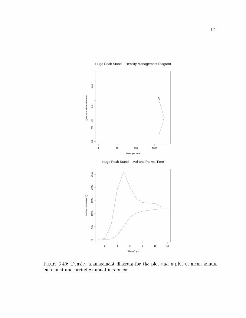
171

*

**

*

*******

*

Trees per acre

Qua

drat

ic M

ean

Dia

met

er

1 10 100 1000

0.1

0.5

1.0

5.0

50.0

Hugo Peak Stand - Density Management Diagram

Time (5 yr)

Mai

and

Pai

(cu

bic

ft)

2 4 6 8 10 12

050

010

0015

0020

0025

00

Hugo Peak Stand - Mai and Pai vs. Time

Figure 6.40: Density management diagram for the plot and a plot of mean annualincrement and periodic annual increment.

172

Time (5 yr)

Fol

iage

Sum

(sq

ft)

2 4 6 8 10 12

010

0000

2000

0030

0000

4000

0050

0000

Hugo Peak Stand - Foliage Sum vs. Time

Growing Stock (cubic ft)

Gro

wth

(cu

bic

ft)

0 20000 40000 60000

050

010

0015

0020

0025

00

Hugo Peak Stand - Growth over Growing Stock

Figure 6.41: A plot of the stand foliage sum over time and a plot of growth overgrowing stock.

173

6.8.3 Hugo Peak Stand, planted origin, 200 trees per acre

In this run, the simulation represents the original intention of the planted stand. It

assumes that 200 trees per acre were planted and the stand is grown with no other

regeneration allowed to enter the stand. The di�erences are very evident in the stand

maps and pro�les (Figures 6.39 and 6.40). The crowns maintain longer lengths and

the widths are more uniform.

Another di�erence is that the density management diagram shows no mortality

and the mean annual increment and periodic annual increment are much further from

culmination that in the �rst two runs (Figure 6.53).

174

Feet

20 40 60 80

2040

6080

Fee

t

* * * * ** *

* * * * * * *

* * * ** * *

* * ** * * *

* * * * * **

* * * * **

Stand Map of Hugo Peak Stand at age 5

feet

20 40 60 80

2040

6080

Fee

t

* * * * ** *

* * * * * * *

* * * ** * *

* * ** * * *

* * * * * **

* * * * **

Stand Map of Hugo Peak Stand at age 25

Feet

20 40 60 80

2040

6080

Fee

t

* * * * ** *

* * * * * * *

* * * ** * *

* * ** * * *

* * * * * **

* * * * **

Stand Map of Hugo Peak Stand at age 45

Feet

20 40 60 80

2040

6080

Fee

t

* * * * ** *

* * * * * * *

* * * ** * *

* * ** * * *

* * * * * **

* * * * **

Stand Map of Hugo Peak Stand at age 60

Figure 6.42: Stand maps at starting year, 25 years after start, 45 years after start,and 60 years after start

175

Distance (ft)

Hei

ght (

ft)

-20 0 20 40 60 80 100 120

020

4060

80

Stand Profile of Hugo Peak Stand at age 5

Distance (ft)

Hei

ght (

ft)

-20 0 20 40 60 80 100 120

020

4060

80

Stand Profile of Hugo Peak Stand at age 25

Distance (ft)

Hei

ght (

ft)

-20 0 20 40 60 80 100 120

020

4060

80

Stand Profile of Hugo Peak Stand at age 45

Distance (ft)

Hei

ght (

ft)

0 50 100

020

4060

8010

0

Stand Profile of Hugo Peak Stand at age 60

Figure 6.43: Stand pro�le at starting year, 25 years after start, 45 years after start,and 60 years after start

176

Hugo Peak Stand - Tree 16

Time (5 yr)

Hei

ght (

ft)

020

4060

8010

012

0

1 2 3 4 5 6 7 8 9 10 11 12

************

Diameter growth for tree 16

Rings are 5 years apart in inchesRadius (in)

Rad

ius

(in)

-20 -10 0 10 20

-20

-10

010

20

Figure 6.44: Tree pro�le and diameter growth for a dominant tree. The radii are ininches and the concentric circles denote �ve year radial growth.

177

Hugo Peak Stand - Tree 18

Time (5 yr)

Hei

ght (

ft)

020

4060

8010

012

0

1 2 3 4 5 6 7 8 9 10 11 12

************

Diameter growth for tree 18

Rings are 5 years apart in inchesRadius (in)

Rad

ius

(in)

-20 -10 0 10 20

-20

-10

010

20

Figure 6.45: Tree pro�le and diameter growth for a co-dominant tree. The radii arein inches and the concentric circles denote �ve year radial growth.

178

Hugo Peak Stand - Tree 4

Time (5 yr)

Hei

ght (

ft)

020

4060

8010

012

0

1 2 3 4 5 6 7 8 9 10 11 12

************

Diameter growth for tree 4

Rings are 5 years apart in inchesRadius (in)

Rad

ius

(in)

-20 -10 0 10 20

-20

-10

010

20

Figure 6.46: Tree pro�le and diameter growth for an intermediate tree. The radiiare in inches and the concentric circles denote �ve year radial growth. In the currentversion there is not threshold for crown size below with a tree cannot survive.

179

Time (5 yr)

Dia

met

er a

t bre

ast h

eigh

t (in

)

2 4 6 8 10 12

010

2030

4050

Hugo Peak Stand - Diameter vs. Time

Time (5 yr)

Dia

met

er a

t bre

ast h

eigh

t (in

)

2 4 6 8 10 12

010

2030

Hugo Peak Stand - Diameter vs. Time

Totaldfwhch

Figure 6.47: Diameter growth for each tree over time ( upper plot) and the meandiameter growth of each species (lower plot). df = Douglas-�r, wh = western hemlock,and ch = cherry.

180

Time (5 yr)

Hei

ght (

ft)

2 4 6 8 10 12

020

4060

8010

0

Hugo Peak Stand - Height vs. Time

Time (5 yr)

Hei

ght (

ft)

2 4 6 8 10 12

2040

6080

100

Hugo Peak Stand - Height vs. Time

Totaldfwhch

Figure 6.48: Height growth for each tree over time (upper plot) and the mean heightgrowth of each species (lower plot).

181

Time (5 yr )

Hei

ght t

o cr

own

base

(ft)

2 4 6 8 10 12

020

4060

80

Hugo Peak Stand - Height to crown base vs. Time

Time (5 yr)

Hei

ght t

o cr

own

base

(ft)

2 4 6 8 10 12

020

4060

80

Hugo Peak Stand - Height to crown base vs. Time

Totaldfwhch

Figure 6.49: Height to crown base change for each tree over time (upper plot) andthe mean height to crown base change for each species (lower plot).

182

Time (5 yr )

Cro

wn

wid

th (

ft)

2 4 6 8 10 12

010

2030

4050

60

Hugo Peak Stand - Crown width vs. Time

Time (5 yr)

Cro

wn

wid

th (

ft)

2 4 6 8 10 12

1020

3040

Hugo Peak Stand - Crown width vs. Time

Totaldfwhch

Figure 6.50: Crown width for each tree over time (upper plot) and the mean crownwidth for each species (lower plot).

183

Time(5 yr)

Fol

iage

sur

face

are

a (s

q ft)

2 4 6 8 10 12

020

0040

0060

0080

0010

000

Hugo Peak Stand - Foliage surface area vs. Time

Time (5 yr)

Fol

iage

sur

face

are

a (s

q ft)

2 4 6 8 10 12

010

0020

0030

0040

00

Hugo Peak Stand - Foliage surface area vs. Time

Totaldfwhch

Figure 6.51: Foliage leaf area for each tree over time (upper plot) and the mean foliageleaf area for each species (lower plot).

184

Time (5 yr)

Hei

ght/d

iam

eter

(P

erce

nt)

2 4 6 8 10 12

020

0040

0060

00

Hugo Peak Stand - Height/diameter vs. Time

In english unitsTime

hd

2 4 6 8 10 12

020

040

060

080

010

0012

0014

00

Hugo Peak Stand - hd vs. Time

Totaldfwhch

Figure 6.52: Height/diameter ratio change for each tree over time (upper plot) andthe mean height/diameter ratio for each species (lower plot).

185

.....

....

.....

....

.....

....

.

...

....

.

.

.

.

..

Rank

Rel

ativ

e ht

0 10 20 30 40

02

46

Time 1

......................................

...

Rank

Rel

ativ

e ht

0 10 20 30 400

510

1520

Time 2

.....

.........

......

...........

....

.

..

...

Rank

Rel

ativ

e ht

0 10 20 30 40

010

2030

Time 3

.............

.......

...........

....

.

.

.

...

Rank

Rel

ativ

e ht

0 10 20 30 40

010

2030

40

Time 4

...........

.........

...........

....

.

..

...

Rank

Rel

ativ

e ht

0 10 20 30 40

010

2030

4050

60

Time 5

................

..............

.....

.

.

....

Rank

Rel

ativ

e ht

0 10 20 30 40

020

4060

Time 6

....

....

.....................

.....

.

.

.

....

Rank

Rel

ativ

e ht

0 10 20 30 40

020

4060

80

Time 7

....

...............................

.

.

....

Rank

Rel

ativ

e ht

0 10 20 30 40

020

4060

80

Time 8

................

................

....

.

....

Rank

Rel

ativ

e ht

0 10 20 30 40

020

4060

80

Time 9

....

...............................

.

.

....

Rank

Rel

ativ

e ht

0 10 20 30 40

020

4060

8010

0

Time 10

...............................

....

.

.

....

Rank

Rel

ativ

e ht

0 10 20 30 40

020

4060

8010

0

Time 11

...................................

.

.

....

Rank

Rel

ativ

e ht

0 10 20 30 40

020

4060

8010

0

Time 12

Figure 6.53. Plot of ordered trees over time. The order time is time 1

186

4.0 5.0 6.0

01

23

45

Height (ft)

Num

ber

Time 1

12 14 16 18 20

02

46

810

Height (ft)

Num

ber

Time 2

20 25 30

02

46

810

12

Height (ft)

Num

ber

Time 3

30 35 40 45

02

46

810

12

Height (ft)

Num

ber

Time 4

40 45 50 55

02

46

810

Height (ft)

Num

ber

Time 5

50 55 60 65 70

02

46

810

12

Height (ft)

Num

ber

Time 6

60 65 70 75 80

05

1015

Height (ft)

Num

ber

Time 7

70 75 80 85

05

1015

Height (ft)N

umbe

r

Time 8

75 80 85 90

05

1015

Height (ft)

Num

ber

Time 9

80 85 90 95 100

05

1015

Height (ft)

Num

ber

Time 10

85 90 95 100 105

05

1015

Height (ft)

Num

ber

Time 11

90 95 100 110

05

1015

Height (ft)

Num

ber

Time 12

Figure 6.54. Histograms of tree height over time.

187

df wh ch

010

2030

Time 1

df wh ch0

1020

30

Time 2

df wh ch

010

2030

Time 3

df wh ch

010

2030

Time 4

df wh ch

010

2030

Time 5

df wh ch

010

2030

Time 6

df wh ch

010

2030

Time 7

df wh ch

010

2030

Time 8

df wh ch

010

2030

Time 9

df wh ch

010

2030

Time 10

df wh ch

010

2030

Time 11

df wh ch

010

2030

Time 12

Figure 6.55. Histogram of species number over time.

188

*

**

*

*

*******

Trees per acre

Qua

drat

ic M

ean

Dia

met

er

1 10 100 1000

0.1

0.5

1.0

5.0

50.0

Hugo Peak Stand - Density Management Diagram

In english unitsTime

Mai

and

Pai

2 4 6 8 10 12

050

010

0015

00

Hugo Peak Stand - Mai and Pai vs. Time

Figure 6.56: Density management diagram for the plot and a plot of mean annualincrement and periodic annual increment.

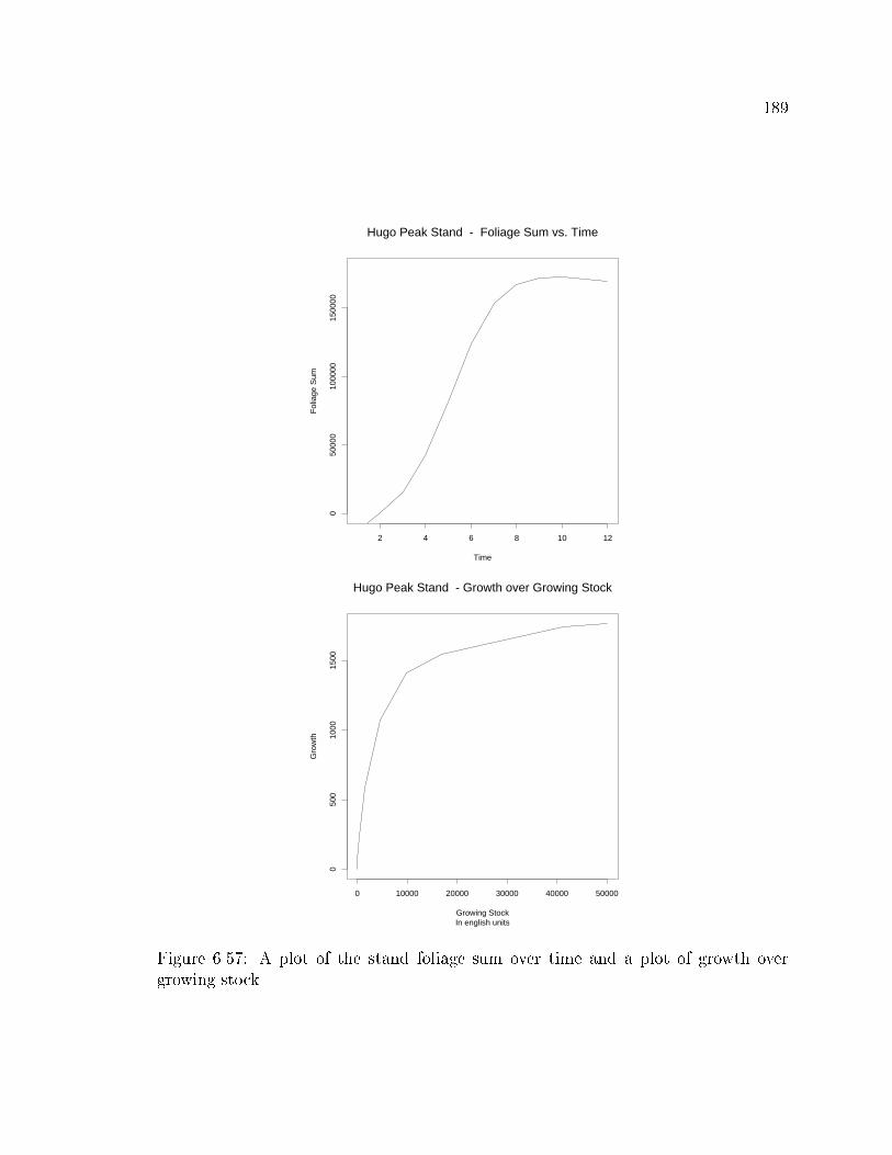
189

Time

Fol

iage

Sum

2 4 6 8 10 12

050

000

1000

0015

0000

Hugo Peak Stand - Foliage Sum vs. Time

In english unitsGrowing Stock

Gro

wth

0 10000 20000 30000 40000 50000

050

010

0015

00

Hugo Peak Stand - Growth over Growing Stock

Figure 6.57: A plot of the stand foliage sum over time and a plot of growth overgrowing stock.

190

6.8.4 Hugo Peak Stand, planted origin, 200 trees per acre with regeneration

This model run represents the actual sequence of events that the original stand under-

went and produces a stand most similar to the actual. In this run, a stand is planted

to 200 trees per acre and regeneration is allowed. The surviving regeneration is near

the edge of the stand, producing a \doughnut" e�ect in the stand maps later in the

growth period (Figure 6.55).

Some interesting species dynamics can be seen in the plots of the mean growth

by species over time. The height histograms over time show a pattern that is similar

to what might be seen in the original stand (Figure 6.66). The species mix changes

even greater because of the di�erential survival parameters for the di�erent species

(Figure 6.67). The ingrowth is apparent in the density management diagram (Figure

6.68). The solid line in this diagram is a stand density index of 595, which is con-

sidered the maximum for Douglas-�r. The model is predicting densities higher that

observed, but the behavior of the stand has been simulated with only the simplest of

mortality assumptions. Additionally, this stand is even further than the other runs

from culmination.

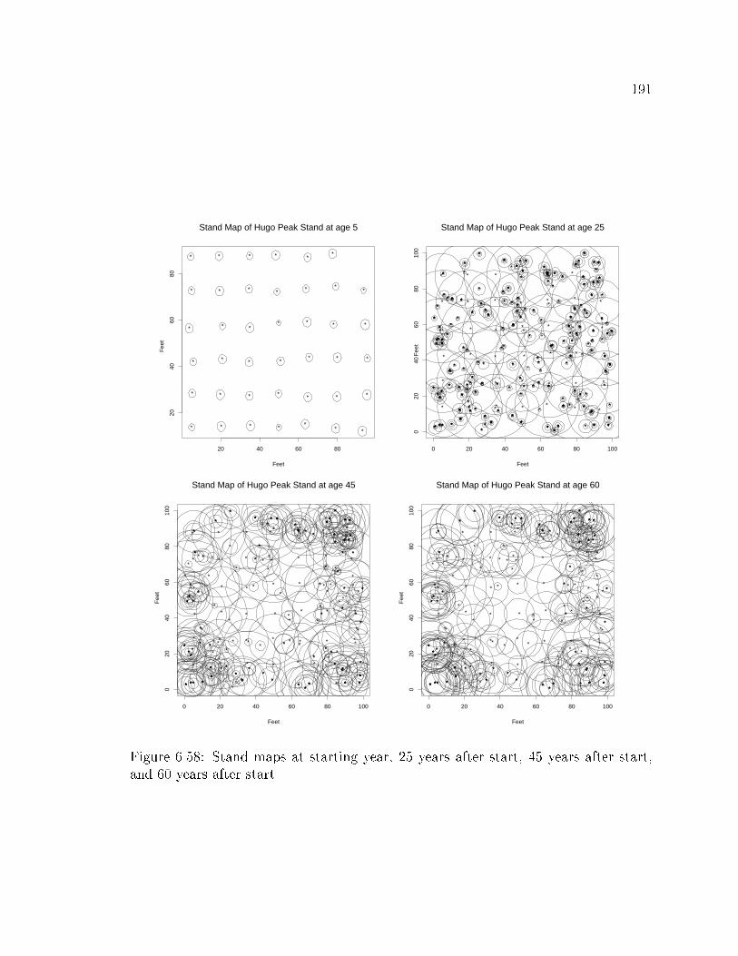
191

Feet

20 40 60 80

2040

6080

Fee

t

* * * * ** *

* * * * * * *

* * * ** * *

* * ** * * *

* * * * * **

* * * * **

Stand Map of Hugo Peak Stand at age 5

Feet

0 20 40 60 80 100

020

4060

8010

0F

eet

* * * * * * *

* * * * * * *

* * * * * * *

* * ** * * *

* * * * * * *

* * * * * *

*

*

*

*

*

*

*

*

*

* *

*

*

**

*

**

*

*

*

**

*

*

*

*

*

**

*

*

*

*

*

*

*

*

*

*

*

*

*

*

*

*

*

*

*

*

*

*

*

**

*

*

*

**

*

*

*

*

*

*

*

*

*

*

*

*

*

*

*

*

*

*

*

*

*

*

**

*

*

*

**

*

*

*

*

*

*

*

*

*

*

*

*

***

*

*

*

*

**

*

*

*

**

*

*

*

*

*

*

*

*

*

*

*

*

*

*

*

*

*

*

*

**

*

*

*

*

*

*

**

*

*

*

*

*

**

*

*

*

*

*

*

*

*

*

*

*

*

*

**

*

*

*

*

*

*

*

*

*

*

**

*

*

*

*

**

*

*

*

*

*

*

*

*

*

*

*

*

*

*

*

*

*

*

*

*

*

*

*

*

*

*

*

**

*

*

*

*

**

*

*

*

*

*

*

*

*

*

*

*

*

*

*

***

*

*

*

*

**

*

*

*

*

**

*

*

*

*

*

*

**

*

*

*

*

***

*

*

*

*

*

*

**

*

*

*

*

*

*

*

*

*

*

*

*

*

*

*

*

*

* *

**

*

*

*

*

*

*

*

*

*

*

*

*

*

* *

*

*

*

*

*

*

*

*

*

*

*

*

*

*

*

*

*

*

*

*

*

*

*

*

*

*

*

**

*

*

*

*

*

*

*

*

*

*

*

*

*

*

*

*

*

*

*

*

*

**

*

*

*

*

*

*

*

*

*

*

*

*

*

**

*

*

*

*

*

*

*

*

*

*

*

*

*

*

***

*

*

*

*

*

*

*

*

*

*

**

*

* *

*

*

*

**

*

*

*

*

*

**

*

*

*

*

*

**

*

*

*

*

*

*

*

*

**

*

*

*

**

*

*

*

*

*

*

*

*

* *

*

**

*

*

*

*

*

*

*

**

*

*

*

*

*

*

*

*

*

*

*

*

*

*

*

*

*

*

*

*

*

*

**

*

*

*

*

*

*

*

*

*

*

*

**

*

* *

*

*

**

*

*

*

*

*

*

*

*

*

*

*

*

*

*

*

*

*

*

*

*

*

*

*

*

*

*

*

*

*

*

*

*

*

*

*

*

*

*

*

**

**

*

*

*

*

**

*

*

*

*

*

*

*

*

*

*

*

*

*

*

*

*

*

*

*

***

*

*

*

*

*

*

*

*

*

*

**

*

*

*

*

*

*

*

*

*

*

*

*

**

*

*

*

*

**

*

*

**

*

*

*

*

*

*

*

*

*

*

*

*

*

*

**

*

**

*

*

*

Stand Map of Hugo Peak Stand at age 25

Feet

0 20 40 60 80 100

020

4060

8010

0

Fee

t

* * * * * * *

* * * * * * *

* * * * * * *

* * ** * * *

* * * * * * *

* * * * * *

*

*

*

*

*

*

* *

*

*

**

*

*

*

*

*

*

*

*

*

*

*

*

*

*

*

*

*

*

*

*

*

*

*

*

*

*

**

*

*

*

**

*

*

*

*

*

*

*

*

*

*

*

*

*

*

*

*

*

*

*

*

*

*

*

*

*

*

*

*

*

*

*

*

***

*

*

*

*

*

*

**

*

*

*

*

*

*

*

*

*

*

*

*

*

*

*

*

**

*

*

*

*

*

*

*

*

**

*

*

*

*

*

*

*

*

*

**

*

*

*

*

*

*

*

*

*

*

**

*

*

*

*

*

*

***

*

**

*

**

*

*

*

*

*

*

*

**

*

*

*

*

*

*

* *

*

*

*

*

*

*

*

*

*

*

*

*

*

*

*

**

*

*

* *

*

*

*

*

**

*

*

*

*

*

*

*

*

*

*

*

*

*

*

*

***

*

*

**

*

*

*

*

*

*

*

*

*

**

*

*

*

*

*

*

*

*

* *

**

*

**

*

*

*

*

*

*

*

*

*

**

**

*

*

*

*

*

*

*

*

*

*

*

***

*

*

*

*

*

** *

*

*

*

*

*

Stand Map of Hugo Peak Stand at age 45

Feet

0 20 40 60 80 100

020

4060

8010

0

Fee

t

* * * * * * *

* * * * * * *

* * * * * * *

* * ** * * *

* * * * * * *

* * * * * *

*

*

*

*

*

*

* *

*

*

**

*

*

*

*

*

*

*

*

*

*

*

*

*

*

*

*

*

*

*

*

*

*

*

*

**

*

*

*

**

*

*

*

*

*

*

*

*

*

*

*

*

*

*

*

*

*

*

*

*

*

*

*

*

*

*

*

*

*

*

*

***

*

*

*

*

*

*

**

*

*

*

*

*

*

*

**

*

*

*

*

*

*

*

*

*

*

**

*

*

*

*

*

*

*

*

**

*

*

*

*

*

*

*

*

**

*

*

*

*

*

***

*

**

*

**

*

*

*

*

*

*

*

**

*

*

*

*

*

* *

*

*

*

*

*

*

*

*

*

*

*

*

*

**

*

*

*

*

*

*

*

**

*

*

*

*

*

*

*

*

*

*

*

*

*

*

*

***

*

*

**

*

*

*

*

*

*

*

*

**

*

*

*

*

*

*

**

** *

*

*

*

*

*

*

*

**

*

*

*

*

*

*

*

*

***

*

*

*

** *

*

*

*

*

Stand Map of Hugo Peak Stand at age 60

Figure 6.58: Stand maps at starting year, 25 years after start, 45 years after start,and 60 years after start.

192

Distance (ft)

Hei

ght (

ft)

-20 0 20 40 60 80 100 120

020

4060

80

Stand Profile of Hugo Peak Stand at age 5

Distance (ft)

Hei

ght (

ft)

-20 0 20 40 60 80 100 120

020

4060

8010

0

Stand Profile of Hugo Peak Stand at age 25

Distance (ft)

Hei

ght (

ft)

-20 0 20 40 60 80 100 120

020

4060

8010

0

Stand Profile of Hugo Peak Stand at age 45

Distance (ft)

Hei

ght (

ft)

0 50 100

020

4060

8010

0

Stand Profile of Hugo Peak Stand at age 60

Figure 6.59: Stand pro�le at starting year, 25 years after start, 45 years after start,and 60 years after start.

193

Hugo Peak Stand - Tree 37

Time (5 yr)

Hei

ght (

ft)

020

4060

8010

012

0

1 2 3 4 5 6 7 8 9 10 11 12

************

Diameter growth for tree 37

Rings are 5 years apart in inchesRadius (in)

Rad

ius

(in)

-20 -10 0 10 20

-20

-10

010

20

Figure 6.60: Tree pro�le and diameter growth for a dominant tree. The radii are ininches and the concentric circles denote �ve year radial growth.

194

Hugo Peak Stand - Tree 26

Time (5 yr)

Hei

ght (

ft)

020

4060

8010

012

0

1 2 3 4 5 6 7 8 9 10 11 12

************

Diameter growth for tree 26

Rings are 5 years apart in inchesRadius (in)

Rad

ius

(in)

-20 -10 0 10 20

-20

-10

010

20

Figure 6.61: Tree pro�le and diameter growth for a co-dominant tree. The radii arein inches and the concentric circles denote �ve year radial growth.

195

Hugo Peak Stand - Tree 24

Time (5 yr)

Hei

ght (

ft)

020

4060

8010

012

0

1 2 3 4 5 6 7 8 9 10 11 12

************

Diameter growth for tree 24

Rings are 5 years apart in inchesRadius (in)

Rad

ius

(in)

-20 -10 0 10 20

-20

-10

010

20

Figure 6.62: Tree pro�le and diameter growth for an intermediate tree. The radii arein inches and the concentric circles denote �ve year radial growth.

196

Time (5 yr)

Dia

met

er a

t bre

ast h

eigh

t (in

)

2 4 6 8 10 12

010

2030

40

Hugo Peak Stand - Diameter vs. Time

Time (5 yr)

Dia

met

er a

t bre

ast h

eigh

t (in

)

2 4 6 8 10 12

02

46

810

1214

Hugo Peak Stand - Diameter vs. Time

Totaldfwhch

Figure 6.63: Diameter growth for each tree over time (upper plot) and the meandiameter growth of each species (lower plot). df = Douglas-�r, wh = western hemlock,and ch = cherry.

197

Time (5 yr)

Hei

ght (

ft)

2 4 6 8 10 12

020

4060

8010

0

Hugo Peak Stand - Height vs. Time

Time (5 yr)

Hei

ght (

ft)

2 4 6 8 10 12

020

4060

80

Hugo Peak Stand - Height vs. Time

Totaldfwhch

Figure 6.64: Height growth for each tree over time (upper plot) and the mean heightgrowth of each species (lower plot).

198

Time (5 yr)

Hei

ght t

o cr

own

base

(ft)

2 4 6 8 10 12

020

4060

80

Hugo Peak Stand - Height to crown base vs. Time

Time (5 yr)

Hei

ght t

o cr

own

base

(ft)

2 4 6 8 10 12

020

4060

Hugo Peak Stand - Height to crown base vs. Time

Totaldfwhch

Figure 6.65: Height to crown base change for each tree over time (upper plot) andthe mean height to crown base change for each species (lower plot).

199

Time (5 yr)

Cro

wn

wid

th (

ft)

2 4 6 8 10 12

010

2030

4050

Hugo Peak Stand - Crown width vs. Time

Time (5 yr)

Cro

wn

wid

th (

ft)

2 4 6 8 10 12

510

15

Hugo Peak Stand - Crown width vs. Time

Totaldfwhch

Figure 6.66: Crown width for each tree over time (upper plot) and the mean crownwidth for each species (lower plot).

200

Time (5 yr)

Fol

iage

sur

face

are

a (s

q ft)

2 4 6 8 10 12

020

0040

0060

0080

00

Hugo Peak Stand - Foliage surface area vs. Time

Time (5 yr)

Fol

iage

sur

face

are

a (s

q ft)

2 4 6 8 10 12

050

010

0015

00

Hugo Peak Stand - Foliage surface area vs. Time

Totaldfwhch

Figure 6.67: Foliage leaf area for each tree over time (upper plot) and the mean foliageleaf area for each species (lower plot).

201

Time (5 yr)

Hei

ght/d

iam

eter

(P

erce

nt)

2 4 6 8 10 12

020

0040

0060

00

Hugo Peak Stand - Height/diameter vs. Time

Figure 6.68. Height/diameter ratio change for each tree over time.

202

4.0 5.0 6.0

01

23

45

Height (ft)

Num

ber

Time 1

0 5 10 15 20

010

020

030

0

Height (ft)

Num

ber

Time 2

0 10 20 30

020

040

060

0

Height (ft)

Num

ber

Time 3

0 10 20 30 40 50

020

040

060

0

Height (ft)

Num

ber

Time 4

0 10 30 50

010

020

030

040

0

Height (ft)

Num

ber

Time 5

0 20 40 60

050

100

150

200

Height (ft)

Num

ber

Time 6

0 20 40 60 80

020

4060

8012

0

Height (ft)

Num

ber

Time 7

0 20 40 60 80

020

4060

80

Height (ft)N

umbe

r

Time 8

0 20 40 60 80 100

020

4060

80

Height (ft)

Num

ber

Time 9

20 40 60 80 100

020

4060

80

Height (ft)

Num

ber

Time 10

20 40 60 80 100

020

4060

80

Height (ft)

Num

ber

Time 11

40 60 80 100 120

020

4060

80

Height (ft)

Num

ber

Time 12

Figure 6.69. Histograms of tree height over time.

203

df wh ch

010

2030

Time 1

df wh ch

050

100

150

Time 2

df wh ch

010

020

030

0

Time 3

df wh ch

010

020

030

0

Time 4

df wh ch

010

020

030

0

Time 5

df wh ch

050

150

250

Time 6

df wh ch

050

150

250

Time 7

df wh ch

050

150

250

Time 8

df wh ch

050

150

Time 9

df wh ch

050

100

200

Time 10

df wh ch

050

100

200

Time 11

df wh ch

050

100

200

Time 12

Figure 6.70. Histogram of species number over time.

204

*

* *

*

*

*

**

****

Trees per acre

Qua

drat

ic M

ean

Dia

met

er

1 10 100 1000

0.1

0.5

1.0

5.0

50.0

Hugo Peak Stand - Density Management Diagram

Time (5 yr)

Mai

and

Pai

(cu

bic

ft)

2 4 6 8 10 12

050

010

0015

0020

0025

00

Hugo Peak Stand - Mai and Pai vs. Time

Figure 6.71: Density management diagram for the plot and a plot of mean annualincrement and periodic annual increment.

205

Time (5 yr)

Fol

iage

Sum

(sq

ft)

2 4 6 8 10 12

010

0000

2000

0030

0000

4000

00

Hugo Peak Stand - Foliage Sum vs. Time

Growing Stock (cubic ft)

Gro

wth

(cu

bic

ft)

0 10000 20000 30000 40000 50000 60000

050

010

0015

0020

0025

00

Hugo Peak Stand - Growth over Growing Stock

Figure 6.72: A plot of the stand foliage sum over time and a plot of growth overgrowing stock.

206

6.8.5 Bethel Ridge Stand

This stand is included as an example of a stand measured in metric units with similar

conditions to the Hugo Peak stand, but a little older. The example was run with no

regeneration allowed. The behavior of the stand follow the general pattern found in

the Hugo peak runs. Again the maps show the thinning of the crowns in the center

of the stand because of the greater amount of competition. Interestingly, the height

distributions remain relatively consistent shape throughout the entire run.

The Bethel Ridge stand was include to illustrate several points. First, the model

can be parameterized with metric data as easily as with English units. Additionally,

it was included to illustrate the type of data that can be used to produce parameter

estimates.

207

Meters

0 10 20 30 40 50

010

2030

4050

Met

ers

*

*

*

*

* *

*

**

*

*

*

*

*

*

*

*

*

*

*

*

*

*

*

*

*

*

*

*

*

*

*

*

**

*

*

*

*

***

*

*

*

*

*

*

*

*

* *

*

*

*

*

*

**

*

*

*

*

*

*

*

*

*

*

* *

*

*

*

*

*

*

*

*

*

*

*

*

*

*

*

*

*

*

**

*

*

*

*

**

*

*

*

*

*

*

*

*

*

*

*

*

*

*

*

*

*

*

*

*

*

*

*

*

*

*

*

*

*

*

*

**

*

*

*

*

*

*

**

*

*

*

*

*

*

*

*

*

*

**

*

*

*

*

*

*

*

*

*

*

*

*

*

*

*

*

*

*

*

* *

*

*

*

*

*

*

*

*

*

*

*

*

*

*

*

*

**

*

**

*

*

*

* *

*

* **

*

*

*

*

*

*

*

*

*

*

*

*

**

*

*

*

*

*

**

*

*

*

*

**

Stand Map of Bethel Ridge Stand at age 5

Meters

0 10 20 30 40 50

010

2030

4050

Met

ers

*

*

*

*

* *

*

**

*

*

*

*

*

*

*

*

*

*

*

*

*

*

*

*

*

*

*

*

*

*

*

*

**

*

*

*

*

***

*

*

*

*

*

*

*

*

* *

*

*

*

*

*

**

*

*

*

*

*

*

*

*

*

*

* *

*

*

*

*

*

*

*

*

*

*

*

*

*

*

*

*

*

*

**

*

*

*

*

**

*

*

*

*

*

*

*

*

*

*

*

*

*

*

*

*

*

*

*

*

*

*

*

*

*

*

*

*

*

*

*

**

*

*

*

*

*

*

**

*

*

*

*

*

*

*

*

*

*

**

*

*

*

*

*

*

*

*

*

*

*

*

*

*

*

*

*

*

*

* *

*

*

*

*

*

*

*

*

*

*

*

*

*

*

*

*

**

*

**

*

*

*

* *

*

* **

*

*

*

*

*

*

*

*

*

*

*

*

**

*

*

*

*

*

**

*

*

*

*

**

Stand Map of Bethel Ridge Stand at age 25

Meters

0 10 20 30 40 50

010

2030

4050

Met

ers

*

*

*

*

* *

*

**

*

*

*

*

*

*

*

*

*

*

*

*

*

*

*

*

*

*

*

*

*

*

*

*

**

*

*

*

*

***

*

*

*

*

*

*

*

*

* *

*

*

*

*

*

**

*

*

*

*

*

*

*

*

*

*

* *

*

*

*

*

*

*

*

*

*

*

*

*

*

*

*

*

*

*

**

*

*

*

*

**

*

*

*

*

*

*

*

*

*

*

*

*

*

*

*

*

*

*

*

*

*

*

*

*

*

*

*

*

*

*

*

**

*

*

*

*

*

*

**

*

*

*

*

*

*

*

*

*

*

**

*

*

*

*

*

*

*

*

*

*

*

*

*

*

*

*

*

*

*

* *

*

*

*

*

*

*

*

*

*

*

*

*

*

*

*

*

**

*

**

*

*

*

* *

*

* **

*

*

*

*

*

*

*

*

*

*

*

*

**

*

*

*

*

*

**

*

*

*

*

**

Stand Map of Bethel Ridge Stand at age 45

Meters

0 10 20 30 40 50

010

2030

4050

Met

ers

*

*

*

*

* *

*

**

*

*

*

*

*

*

*

*

*

*

*

*

*

*

*

*

*

*

*

*

*

*

*

*

**

*

*

*

*

***

*

*

*

*

*

*

*

*

* *

*

*

*

*

*

**

*

*

*

*

*

*

*

*

*

*

* *

*

*

*

*

*

*

*

*

*

*

*

*

*

*

*

*

*

*

**

*

*

*

*

**

*

*

*

*

*

*

*

*

*

*

*

*

*

*

*

*

*

*

*

*

*

*

*

*

*

*

*

*

*

*

*

**

*

*

*

*

*

*

**

*

*

*

*

*

*

*

*

*

*

**

*

*

*

*

*

*

*

*

*

*

*

*

*

*

*

*

*

*

*

* *

*

*

*

*

*

*

*

*

*

*

*

*

*

*

*

*

**

*

**

*

*

*

* *

*

* **

*

*

*

*

*

*

*

*

*

*

*

*

**

*

*

*

*

*

**

*

*

*

*

**

Stand Map of Bethel Ridge Stand at age 60

Figure 6.73: Stand maps at starting year, 25 years after start, 45 years after start,and 60 years after start.

208

Distance (m)

Hei

ght (

m)

-20 0 20 40 60

010

2030

4050

Stand Profile of Bethel Ridge Stand at age 5

Distance (m)

Hei

ght (

m)

-20 0 20 40 60

010

2030

4050

Stand Profile of Bethel Ridge Stand at age 25

Distance (m)

Hei

ght (

m)

-20 0 20 40 60

010

2030

4050

Stand Profile of Bethel Ridge Stand at age 45

Distance (m)

Hei

ght (

m)

-20 0 20 40 60

010

2030

4050

Stand Profile of Bethel Ridge Stand at age 60

Figure 6.74: Stand pro�le at starting year, 25 years after start, 45 years after start,and 60 years after start.

209

Bethel Ridge Stand - Tree 201

Time (5 yr)

Hei

ght (

m)

010

2030

4050

60

1 2 3 4 5 6 7 8 9 10 11 12

************

Diameter growth for tree 201

Rings are 5 years apart in centimetersRadius (cm)

Rad

ius

(cm

)

-20 -10 0 10 20

-20

-10

010

20

Figure 6.75: Tree pro�le and diameter growth for a dominant tree. The radii are incentimeters. The concentric circle denote �ve year radial growth.

210

Bethel Ridge Stand - Tree 205

Time (5 yr)

Hei

ght (

m)

010

2030

4050

60

1 2 3 4 5 6 7 8 9 10 11 12

************

Diameter growth for tree 205

Rings are 5 years apart in centimetersRadius (cm)

Rad

ius

(cm

)

-20 -10 0 10 20

-20

-10

010

20

Figure 6.76: Tree pro�le and diameter growth for a co-dominant tree. The radii arein centimeters. The concentric circle denote �ve year radial growth.

211

Bethel Ridge Stand - Tree 153

Time (5 yr)

Hei

ght (

m)

010

2030

4050

60

1 2 3 4 5 6 7 8 9 10 11 12

************

Diameter growth for tree 153

Rings are 5 years apart in centimetersRadius (cm)

Rad

ius

(cm

)

-20 -10 0 10 20

-20

-10

010

20

Figure 6.77: Tree pro�le and diameter growth for an intermediate tree. The radii arein centimeters. The concentric circle denote �ve year radial growth.

212

Time (5 yr)

Dia

met

er a

t bre

ast h

eigh

t (cm

)

2 4 6 8 10 12

010

2030

40

Bethel Ridge Stand - Diameter vs. Time

Time (5 yr)

Dia

met

er a

t bre

ast h

eigh

t (cm

)

2 4 6 8 10 12

05

1015

20

Bethel Ridge Stand - Diameter vs. Time

Totalpsmetshe

Figure 6.78: Diameter growth for each tree over time (upper plot) and the meandiameter growth of each species (lower plot). psme = Douglas-�r, and tshe = westernhemlock.

213

Time (5 yr)

Hei

ght (

m)

2 4 6 8 10 12

1020

30

Bethel Ridge Stand - Height vs. Time

Time (5 yr)

Hei

ght (

m)

2 4 6 8 10 12

1020

30

Bethel Ridge Stand - Height vs. Time

Totalpsmetshe

Figure 6.79: Height growth for each tree over time (upper plot) and the mean heightgrowth of each species (lower plot).

214

Time (5 yr)

Hei

ght t

o cr

own

base

(m

)

2 4 6 8 10 12

010

2030

Bethel Ridge Stand - Height to crown base vs. Time

Time (5 yr)

Hei

ght t

o cr

own

base

(m

)

2 4 6 8 10 12

05

1015

2025

30

Bethel Ridge Stand - Height to crown base vs. Time

Totalpsmetshe

Figure 6.80: Height to crown base change for each tree over time (upper plot) andthe mean height to crown base change for each species (lower plot).

215

Time (5 yr)

Cro

wn

wid

th (

m)

2 4 6 8 10 12

510

1520

Bethel Ridge Stand - Crown width vs. Time

Time (5 yr)

Cro

wn

wid

th (

m)

2 4 6 8 10 12

24

68

Bethel Ridge Stand - Crown width vs. Time

Totalpsmetshe

Figure 6.81: Crown width for each tree over time (upper plot) and the mean crownwidth for each species (lower plot).

216

Time (5 yr)

Fol

iage

sur

face

are

a (s

q m

)

2 4 6 8 10 12

020

040

060

080

010

00

Bethel Ridge Stand - Foliage surface area vs. Time

Time (5 yr)

Foi

lage

sur

face

are

a (s

q m

)

2 4 6 8 10 12

5010

015

020

0

Bethel Ridge Stand - Foliage surface area vs. Time

Totalpsmetshe

Figure 6.82: Foliage leaf area for each tree over time (upper plot) and the mean foliageleaf area for each species (lower plot).

217

Time (5 yr)

Hei

ght/d

iam

eter

(P

erce

nt)

2 4 6 8 10 12

200

400

600

800

1000

Bethel Ridge Stand - Height/diameter vs. Time

Time (5 yr)

Hei

ght/d

iam

eter

(P

erce

nt)

2 4 6 8 10 12

200

300

400

500

600

Bethel Ridge Stand - Height/diameter vs. Time

Totalpsmetshe

Figure 6.83: Height/diameter ratio change for each tree over time (upper plot) andthe mean height/diameter ratio for each species (lower plot).

218

.

.

.

........

.

.

.............

.

.....

.

.

.

.......

.....

.

.

.

.

........

.

.

.........

.......

...

................

.

.........

.

.

...

.....

.

..

............

......

.

.

.

.

.

.

.

.

.............................................................

.

.

.

...............

.

...

Rank

Rel

ativ

e ht

0 50 100 150 200

01

23

4

Time 1

....................................................................................................................................................................................................................................

Rank

Rel

ativ

e ht

0 50 100 150 200

02

46

8

Time 2

.

..........................................................

.

..........................................................................

.

.

...........................

.............................................................

.

...

Rank

Rel

ativ

e ht

0 50 100 150 200

02

46

810

12

Time 3

.

..........................................................

.

......................................

.

...................

...........................

.....................

.

.............................................................

Rank

Rel

ativ

e ht

0 50 100 150 200

05

1015

Time 4

...........................................................

...........................................................................

.........................

.

.........................

.

.

.

........................

................

Rank

Rel

ativ

e ht

0 50 100 150 200

05

1015

20

Time 5

.................................................................

.................................

.

....................................

..................................................

.

.

.

........................................

Rank

Rel

ativ

e ht

0 50 100 150 200

05

1015

20

Time 6

........................................

..........................................................

.

........................................

..............................................

.

.

.

........................................

Rank

Rel

ativ

e ht

0 50 100 150 200

05

1015

2025

Time 7

..........................................

....................

..........................................

.......................................

.................................

..........................

..........................

RankR

elat

ive

ht

0 50 100 150 200

05

1015

2025

30

Time 8

...............................................

.......................

..................................

.......................................

..............................................................

.......................

Rank

Rel

ativ

e ht

0 50 100 150 200

05

1015

2025

30

Time 9

...........................................................

............................................

..........................................

................................

...................................................

Rank

Rel

ativ

e ht

0 50 100 150 200

010

2030

Time 10

..............................................................

.........................................

....................................................

..............................................................

...........

Rank

Rel

ativ

e ht

0 50 100 150 200

010

2030

Time 11

........................................................................................................

...................................................

.

........................................................................

Rank

Rel

ativ

e ht

0 50 100 150 200

010

2030

Time 12

Figure 6.84. Plot of ordered trees over time. The order time is time 1.

219

2.0 3.0 4.0

010

2030

Height (m)

Num

ber

Time 1

5 6 7 8 90

2040

60

Height (m)

Num

ber

Time 2

8 9 10 11 12 13

020

4060

Height (m)

Num

ber

Time 3

12 13 14 15 16 17

010

2030

4050

60

Height (m)

Num

ber

Time 4

16 17 18 19 20

020

4060

Height (m)

Num

ber

Time 5

19 20 21 22 23 24

010

2030

4050

60

Height (m)

Num

ber

Time 6

23 24 25 26 27

010

2030

4050

60

Height (m)

Num

ber

Time 7

25 26 27 28 29

020

4060

Height (m)

Num

ber

Time 8

28 29 30 31 32

010

2030

4050

60

Height (m)

Num

ber

Time 9

30 31 32 33 34

020

4060

Height (m)

Num

ber

Time 10

33 34 35 36

020

4060

80

Height (m)

Num

ber

Time 11

35 36 37 38

020

4060

80

Height (m)

Num

ber

Time 12

Figure 6.85. Histograms of tree height over time.

220

psme tshe

050

100

150

200

Time 1

psme tshe

050

100

150

200

Time 2

psme tshe

050

100

150

200

Time 3

psme tshe

050

100

150

200

Time 4

psme tshe

050

100

150

200

Time 5

psme tshe

050

100

150

200

Time 6

psme tshe

050

100

150

200

Time 7

psme tshe

050

100

150

200

Time 8

psme tshe

050

100

150

200

Time 9

psme tshe

050

100

150

200

Time 10

psme tshe

050

100

150

200

Time 11

psme tshe

050

100

150

200

Time 12

Figure 6.86. Histogram of species number over time.

221

*

*

*

*

********

Trees per hectare

Qua

drat

ic M

ean

Dia

met

er

1 10 100 1000 10000

15

1050

100

500

Bethel Ridge Stand - Density Management Diagram

Time (5 yr )

Mai

and

Pai

(cu

bic

m)

2 4 6 8 10 12

020

040

060

080

0

Bethel Ridge Stand - Mai and Pai vs. Time

Figure 6.87: Density management diagram for the plot and a plot of mean annualincrement and periodic annual increment.

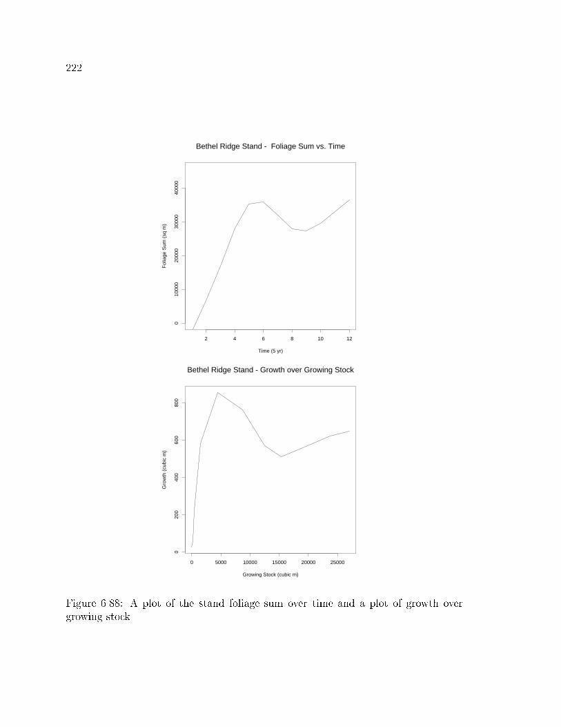
222

Time (5 yr)

Fol

iage

Sum

(sq

m)

2 4 6 8 10 12

010

000

2000

030

000

4000

0

Bethel Ridge Stand - Foliage Sum vs. Time

Growing Stock (cubic m)

Gro

wth

(cu

bic

m)

0 5000 10000 15000 20000 25000

020

040

060

080

0

Bethel Ridge Stand - Growth over Growing Stock

Figure 6.88: A plot of the stand foliage sum over time and a plot of growth overgrowing stock.

223

6.8.6 Helena Plots

The Helena plots illustrate the use of the model with data from a very di�erent

area and very di�erent tree species. The idea is to simulate the stand's history to

try to predict a stand that appeared similar to the one measured. The attempt was

somewhat successful. The assumption of a constant crown length to crown width ratio

is not applicable here, and more dynamic crown assumptions are needed. Outside of

this assumption, the model appears to work reasonably with these data.

In this run, the events of the original experiment were simulated. Four row of

Cherrybark oak were established next to four rows of american sycamore and then

four empty rows representing the space in which cottonwood were planted and died.

The run did re ect the superior height growth of the american sycamore but did

not clearly re ect the di�erential size pattern observed in the original stands (Oliver

et al., 1990).

The height growth patterns di�erentiated between the two species but not enough

variation was input into each species height growth pattern. The cherrybark oak

experienced a higher mortality rate than the sycamore which is re ected in the species

histograms in Figure 6.102.

224

Feet

0 20 40 60 80 100

2040

6080

Fee

t

* * * * * * * * *

* * * * * * * * *

* * * * * * * * *

* * * * * * * * *

* * * * * * * * *

* * * * * * * * *

* * * * * * * * *

* * * * * * * * *

* * * * * * * * *

* * * * * * * * *

* * * * * * * * *

* * * * * * * *

Stand Map of Helena plots

Feet

0 20 40 60 80 100

2040

6080

Fee

t

* * * * * * * * *

* * * * * * * * *

* * * * * * * * *

* * * * * * * * *

* * * * * * * * *

* * * * * * * * *

* * * * * * * * *

* * * * * * * * *

* * * * * * * * *

* * * * * * * * *

* * * * * * * * *

* * * * * * * *

Stand Map of Helena plots

Feet

0 20 40 60 80 100

2040

6080

Fee

t

* * * * * * * *

* * * * * * * * *

* * * * * * * *

* * * * * * *

* * * * * * * *

* * * * * * * *

* * * * * * * * *

* * * * * * *

* * * * * * * * *

* * * * * * * *

* * * * * * * * *

* * * * * * * *

Stand Map of Helena plots

Feet

0 20 40 60 80 100

2040

6080

Fee

t

* * * * * * * *

* * * * * * * * *

* * * * * * * *

* * * * * * *

* * * * * * * *

* * * * * * * *

* * * * * * * * *

* * * * * * *

* * * * * * * * *

* * * * * * *

* * * * * * * * *

* * * * * * * *

Stand Map of Helena plots

Figure 6.89: Stand maps at starting year, 25 years after start, 45 years after start,and 60 years after start. The four rows on the left are cherrybark oak the four centerrows are sycamore and the row on the far right is again cherrybark oak.

225

Distance (ft)

Hei

ght (

ft)

-20 0 20 40 60 80 100 120

020

4060

8010

0

Stand Profile of Helena plots

Distance (ft)

Hei

ght (

ft)

0 50 100

020

4060

8010

0

Stand Profile of Helena plots

Distance (ft)

Hei

ght (

ft)

0 50 100 150

020

4060

8010

012

014

0

Stand Profile of Helena plots

Distance (ft)

Hei

ght (

ft)

0 50 100 150

050

100

150

Stand Profile of Helena plots

Figure 6.90: Stand pro�le at starting year, 25 years after start, 45 years after start,and 60 years after start. The four rows on the left are cherrybark oak the four centerrows are sycamore and the row on the far right is again cherrybark oak.

226

Helena plots - Tree 62

Time (5 yr)

Hei

ght (

ft)

050

100

150

1 2 3 4 5 6 7 8 9 10 11 12

************

Diameter growth for tree 62

Rings are 5 years apart in inchesRadius (in)

Rad

ius

(in)

-20 -10 0 10 20

-20

-10

010

20

Figure 6.91: Tree pro�le and diameter growth for a dominant tree. This tree is asycamore.

227

Helena plots - Tree 75

Time (5 yr)

Hei

ght (

ft)

020

4060

8010

012

014

0

1 2 3 4 5 6 7 8 9 10 11 12

************

Diameter growth for tree 75

Rings are 5 years apart in inchesRadius (in)

Rad

ius

(in)

-20 -10 0 10 20

-20

-10

010

20

Figure 6.92: Tree pro�le and diameter growth for a co-dominant tree. This tree is ancherrybark oak.

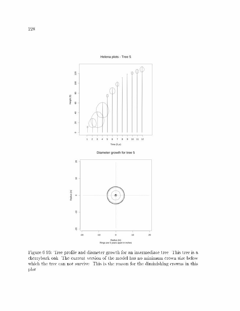
228

Helena plots - Tree 5

Time (5 yr)

Hei

ght (

ft)

020

4060

8010

012

0

1 2 3 4 5 6 7 8 9 10 11 12

************

Diameter growth for tree 5

Rings are 5 years apart in inchesRadius (in)

Rad

ius

(in)

-20 -10 0 10 20

-20

-10

010

20

Figure 6.93: Tree pro�le and diameter growth for an intermediate tree. This tree is acherrybark oak. The current version of the model has no minimum crown size belowwhich the tree can not survive. This is the reason for the diminishing crowns in thisplot.

229

Time (5 yr)

Dia

met

er a

t bre

ast h

eigh

t (in

)

2 4 6 8 10 12

010

2030

40

Helena plots - Diameter vs. Time

Time (5 yr)

Dia

met

er a

t bre

ast h

eigh

t (in

)

2 4 6 8 10 12

510

1520

25

Helena Plots - Diameter vs. Time

Totalsyccbo

Figure 6.94: Diameter growth for each tree over time (upper plot) and the meandiameter growth of each species (lower plot). syc = American sycamore, and cbo =cherrybark oak.

230

Time (5 yr)

Hei

ght (

ft)

2 4 6 8 10 12

2040

6080

100

120

140

160

Helena plots - Height vs. Time

Time (5 yr)

Hei

ght (

ft)

2 4 6 8 10 12

2040

6080

100

120

140

Helena Plots - Height vs. Time

Totalsyccbo

Figure 6.95: Height growth for each tree over time (upper plot) and the mean heightgrowth of each species (lower plot).

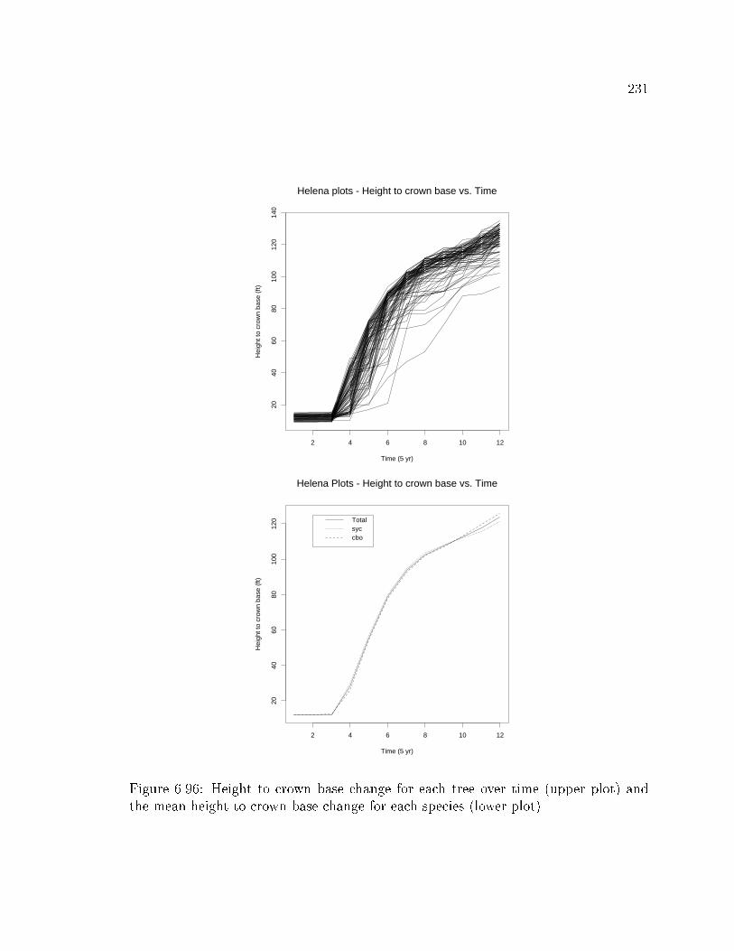
231

Time (5 yr)

Hei

ght t

o cr

own

base

(ft)

2 4 6 8 10 12

2040

6080

100

120

140

Helena plots - Height to crown base vs. Time

Time (5 yr)

Hei

ght t

o cr

own

base

(ft)

2 4 6 8 10 12

2040

6080

100

120

Helena Plots - Height to crown base vs. Time

Totalsyccbo

Figure 6.96: Height to crown base change for each tree over time (upper plot) andthe mean height to crown base change for each species (lower plot).

232

Time (5 yr)

Cro

wn

wid

th (

ft)

2 4 6 8 10 12

010

2030

4050

60

Helena plots - Crown width vs. Time

Time (5 yr)

Cro

wn

wid

th (

ft)

2 4 6 8 10 12

1020

3040

Helena Plots - Crown width vs. Time

Totalsyccbo

Figure 6.97: Crown width for each tree over time (upper plot) and the mean crownwidth for each species (lower plot).

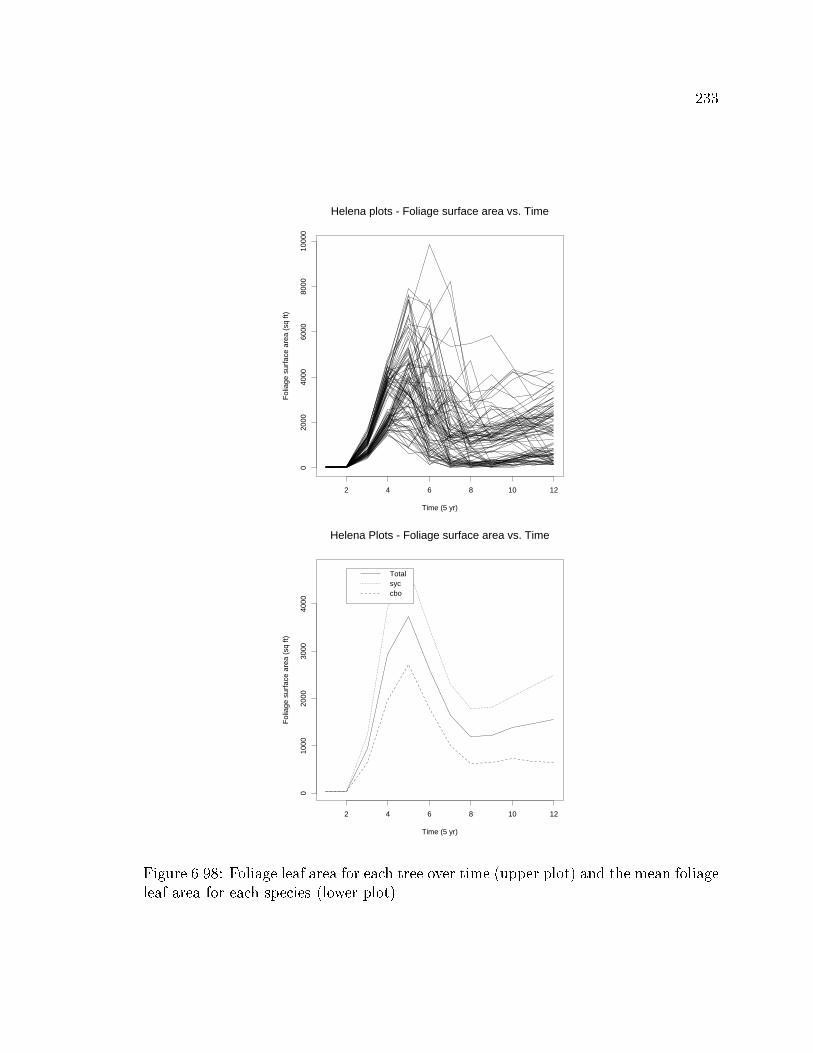
233

Time (5 yr)

Fol

iage

sur

face

are

a (s

q ft)

2 4 6 8 10 12

020

0040

0060

0080

0010

000

Helena plots - Foliage surface area vs. Time

Time (5 yr)

Fol

iage

sur

face

are

a (s

q ft)

2 4 6 8 10 12

010

0020

0030

0040

00

Helena Plots - Foliage surface area vs. Time

Totalsyccbo

Figure 6.98: Foliage leaf area for each tree over time (upper plot) and the mean foliageleaf area for each species (lower plot).

234

Time (5 yr)

Hei

ght/d

iam

eter

(P

erce

nt)

2 4 6 8 10 12

100

200

300

400

Helena plots - Height/diameter vs. Time

Time (5 yr)

Hei

ght/d

iam

eter

(P

erce

nt)

2 4 6 8 10 12

100

150

200

250

300

350

Helena Plots - Height/diameter vs. Time

Totalsyccbo

Figure 6.99: Height/diameter ratio change for each tree over time (upper plot) andthe mean height/diameter ratio for each species (lower plot).

235

.....

.

....

...

.........

......

.

.

.

....

.......

.

.

..

.

.....

....

.......

..

................

.

.....

.........

........

...

Rank

Rel

ativ

e ht

0 20 40 60 80

05

1015

20Time 1

..........................................................................................................

.

Rank

Rel

ativ

e ht

0 20 40 60 800

1020

3040

50

Time 2

..........................

................

.

.

..

.

.....

..........

..............................

...............

Rank

Rel

ativ

e ht

0 20 40 60 80

020

4060

Time 3

.......................................

...

.

.

..

.

.....

....

....................................

...............

Rank

Rel

ativ

e ht

0 20 40 60 80

020

4060

80

Time 4

...........................

...............

.

.

..

.

.....

....

...................................................

Rank

Rel

ativ

e ht

0 20 40 60 80

020

4060

8010

0

Time 5

...................................

.......

.

.

..

.

.....

....

....................................

...............

Rank

Rel

ativ

e ht

0 20 40 60 80

020

4060

8010

0

Time 6

..........................................

.

.

..

.

.....

....

................................

............

.

.....

.

Rank

Rel

ativ

e ht

0 20 40 60 80

020

4060

8010

0

Time 7

..........................................

.

.

..

.

.....

....................................

............

.

.....

.

Rank

Rel

ativ

e ht

0 20 40 60 80

020

4060

8010

0

Time 8

..........................................

.

.

...

.....

.........................

......

.....

..

...

.

......

.

..

.

..

.

Rank

Rel

ativ

e ht

0 20 40 60 80

020

4060

8012

0

Time 9

..........................................

.

.

...

.....

.........................

.

..........

..

...

.

......

.

..

.

..

.

Rank

Rel

ativ

e ht

0 20 40 60 80

020

4060

8012

0

Time 10

..........................................

.

....

.....

.........................

.

....

.

.....

..

...

.

......

.

..

.

..

.

Rank

Rel

ativ

e ht

0 20 40 60 80

050

100

150

Time 11

..........................................

.

...

.

.

.

...

.........................

.

....

.

.....

..

...

.

......

.

..

.

..

.

Rank

Rel

ativ

e ht

0 20 40 60 80

050

100

150

Time 12

Figure 6.100: Plot of ordered trees over time. The order time is time 2. Note the twolevels apparent in these plots

236

12 14 16 18 20

05

1015

2025

Height (ft)

Num

ber

Time 1

25 30 35 40 45 50

02

46

810

1214

Height (ft)

Num

ber

Time 2

40 50 60 70

05

1015

20

Height (ft)

Num

ber

Time 3

60 70 80 90

05

1015

2025

Height (ft)

Num

ber

Time 4

75 85 95 105

05

1015

Height (ft)

Num

ber

Time 5

90 95 105 115

05

1015

Height (ft)

Num

ber

Time 6

100 110 120

05

1015

Height (ft)

Num

ber

Time 7

110 120 130

05

1015

20

Height (ft)N

umbe

r

Time 8

115 125 135

05

1015

20

Height (ft)

Num

ber

Time 9

125 135 145

05

1015

2025

Height (ft)

Num

ber

Time 10

130 135 140 145 150

05

1015

20

Height (ft)

Num

ber

Time 11

135 145 155

05

1015

2025

30

Height (ft)

Num

ber

Time 12

Figure 6.101. Histograms of tree height over time. Note the bimodal distribution.

237

syc cbo

010

2030

4050

60

Time 1

syc cbo0

1020

3040

5060

Time 2

syc cbo

010

2030

4050

60

Time 3

syc cbo

010

2030

4050

60

Time 4

syc cbo

010

2030

4050

60

Time 5

syc cbo

010

2030

4050

Time 6

syc cbo

010

2030

4050

Time 7

syc cbo

010

2030

4050

Time 8

syc cbo

010

2030

4050

Time 9

syc cbo

010

2030

4050

Time 10

syc cbo

010

2030

4050

Time 11

syc cbo

010

2030

4050

Time 12

Figure 6.102. Histogram of species number over time.

238

***

*

********

Trees per acre

Qua

drat

ic M

ean

Dia

met

er

1 10 100 1000

0.1

0.5

1.0

5.0

50.0

Helena plots - Density Management Diagram

Time (5 yr)

Mai

and

Pai

(cu

bic

ft)

2 4 6 8 10 12

050

010

0015

0020

0025

00

Helena plots - Mai and Pai vs. Time

Figure 6.103: Density management diagram for the plot and a plot of mean annualincrement and periodic annual increment.

239

Time (5 yr)

Fol

iage

Sum

(sq

ft)

2 4 6 8 10 12

010

0000

2000

0030

0000

4000

00

Helena plots - Foliage Sum vs. Time

Growing Stock (cubic ft)

Gro

wth

(cu

bic

ft)

0 10000 20000 30000 40000 50000 60000

050

010

0015

0020

0025

00

Helena plots - Growth over Growing Stock

Figure 6.104: A plot of the stand foliage sum over time and a plot of growth overgrowing stock.

240

6.9 Discussion of the approach

The adaptive model of stand dynamics illustrates the potential of this approach; it

has many interesting advantages and disadvantages. Advantages include exibility,

ease of use with very di�erent types of input information, and ease of application

for adaptive silviculture. Disadvantages include an inability to represent some of

the subtler behavior exhibited by the modeled stands. Some of this is because of

the generalizations made by the approach and some of it is because of incompletely

speci�ed submodels. These submodels can be corrected. This inability to explain �ne

detail is to be expected and can be easily accommodated in the adaptive management

approach.

The main advantage of the approach to modeling is exibility. This exibility

however, carries the responsibility of carefully evaluating the output from any sim-

ulations. For example, a new graph of stand values was generated from stand data

within minutes. The exibility is in part because of the statistical package used for

display and in part because of the models modular design. The modularity and ex-

ibility �t well into the adaptive management approach. As functions, output, other

desired information are found lacking, they can be incorporated into future versions

of the model.

Another advantage is the graphical output, which can help a person evaluate a lot

of information quickly. The graphical model interface has been e�ective, and parts

of the graphical interface have been adapted for use with other forest growth models.

Graphical user output is not limited to adaptive models of stand dynamics; but the

output is very useful in accomplishing the objectives of adaptive silviculture.

A third advantage is the relatively few relationships needed to explain behaviors

exhibited in model runs. Twelve deterministic parameters per species are needed to

run this model, and another �fteen stochastic parameters are used to simulate the

static and error distributions in the input data.

241

The predictions reproduce the stands' maximum height growth behavior well. The

current data did not have any other measurements over time to compare to the pre-

dictions. This adaptive stand dynamics model is designed to utilize information from

expert opinions, to single time measurements, to repeated measurements. Only the

single time measurements are used in this dissertation. While adequate to parame-

terize the model and make simulations, the current data are not the best. Repeated

measurements would provide even more useful information that would allow better

parameter sets and more complete evaluation of the model output as the stand be-

comes older.

There are numerous areas of the model that can be improved. A de�nition of

the dynamics of the crown width to crown length is needed to produce more realistic

crowns. This would improve the predictions of hardwood species and possibly conifers.

The current static relationship of crown length to crown width may provide over

estimates of crown size.

The question of mortality should also be addressed. The current method based on

crown competition seems plausible in the early developmental stage of the stand, but

is inadequate in later development. Another area of improvement is the relationship

of foliage area to stem increment. Both this and the previous question would require

independent experiments to determine the best approach to satisfy these questions.

Additional improvement beyond these is probably not be needed, since it would

be beyond the scope of the questions that this type of model would be able to analyze.

These more detailed question would be better answered with detailed models focused

at speci�c questions and from which generalized behaviors can be determined for

stand level models presented here.

Chapter 7

A LARGER FOREST MANAGEMENT SYSTEM

\There are no \bigger secrets" because the moment a secret is revealed, it

seems little."

Umberto Eco, 1988, \Foucault's Pendulum", Chapter 118

The adaptive growth model presented here is only part of a larger forest manage-

ment system. The design of the adaptive stand dynamics model implies that the forest

manager will be monitoring a stand over time and using the additional information

collected at successive measurements to update the parameters of the growth model.

This type of model is designed for managers interested in the long term management

of forest stands.

Along with monitoring, a larger forest management system could integrate many of

the decision making processes into a system of modular pieces, which could be updated

or changed as the the needs of the managers change. One proposed con�guration is

diagrammed in Figure 7.1.

7.1 A proposed larger forest management system

In Figure 7.1, the adaptive growth model is represented by the box in the upper right

corner. All work presented throughout this dissertation would belong in this box.

Inventory and Monitoring - This is probably the most valuable component for all

other components to work well. If managers do not have a good inventory upon

which to base decisions and a monitoring system to provide the information to

243

Evaluator Info.Traditional

Info.Spatial

GIS

Database

SuccessManagement

DocumentorPlan

Management

EvaluatorPattern

LandscapeScheduling

Harvest

EvaluatorAlternative

Management

ModelGrowth

Monitoring&

Inventory

EvaluatorSuccessSystem

Figure 7.1. One possible con�guration of a larger forest management system.

244

evaluate decisions previously made, decisions will be inaccurate. This informa-

tion can also be used to determine the time at which decisions are required. The

monitoring can be keyed to the times in stand development that would probably

require treatment (thinning, fertilization, and others), as opposed to regularly

space intervals in time. Either method should work as long as the monitoring

is consisted, rational, and well documented.

Database - This component of the system provides a data handling function for all

other components. With all components interacting, information about stands

and the relationships between stands must be well organized to be accessible

and useful. The database component provides this function in the forest man-

agement system. The box is divided into two parts, because information about

forests are in both spatial and list form; and a database that handles one form

well seldom handle the others well. A connection between the two databases is

necessary to have a fully functional system.

Alternative treatment generation - Silviculture should be the practice of taking a

set of stands and, with the minimum manipulation, moving the stand to a

set of conditions that meet the management goals for the ownership. When

considering alternative treatments, how is the appropriate treatment chosen?

One approach is to �lter through combinations of alternatives for the stand

conditions, developing possible operations and their cost. Alternatives that can

be generated in this way may have equivalent utility to the manager but have

very di�erent timing of treatments or provide very di�erent stand structure and

landscape patterns. A method of evaluating the selected pattern in terms of

these broader issues is also needed.

Documentation - This is very important in accessing the success of a forest man-

agement system. A recurrent problem in forest management is that stand pre-

245

scriptions are made, �led, and seldom referred to again. The management of

a stand following a prescription should have anticipated outcomes that can be

checked consequently, a good system of record keeping is used. A system of

record keeping should be easy to use, provide useful information to the people

collecting the information, and organized for easy future retrieval.

Success of Management - This component implements a management system idea

in which the performance of the chosen management alternative is evaluated.

This comparison of predicted behavior of the stand and the actual behavior of

the stand provides a needed check with reality. If the the behaviors are similar,

con�dence in the prediction is increased. If the behaviors are di�erent, a decision

must be made whether the actual behavior is acceptable or new operations are

and management direction is needed. The analyzes must be done on a routine

basis, not just when a problem is perceived.

Success of the System - This component could be designed to monitor the per-

formance of the components of the management systems. If portions of the

management system consistently have poor behavior in many di�erent stands,

that part of the system would be a candidate for improvement.

These are a few ways this type of model can be used in the context of a larger

system. Many other project need to be completed to have a working system.

7.2 Some statistical aspects designed into the current approach

The adaptive stand dynamics model has many potential aspects designed or, provided

for, than there is room or time to test or demonstrate in this dissertation. The model

has many of the same elements as traditional forest growth models but it emphasizes

di�erent things. Below is a review of how this type of model di�ers and it describes

why the proposed approach may be useful:

246

� Maximum use from diverse types of information is desired. Under the proposed

scenario, a user would have information and data from such various sources such

as published equations, stem analysis from a stand, stand measurements, repeat

measurements from the same stand, and growth equations from forest-wide

inventories. The models should make maximum use of whatever information or

data are available within the framework proposed for the model.

� A systematic method for updating the model with varying degrees of memory

of the the past values of parameters. When the established parameters are

considered by the user to be good, the model should be able to have a strong

memory. If the parameters of the model are known with less certainty, then

weak memory would be desired as the new information will have more value for

prediction that the old parameter estimates (Berger, 1985; Goldberg, 1989).

� A method of producing an estimate of the cumulative variance from the various

model components is important. Growth models have been built and used that

predict average values with little information about the range of the outcomes

likely to be encountered. This range of outcomes is at least as important that

the mean values. Because one must know something about the likelihood of a

particular outcome to accurately calculate a risk function for decision making.

7.2.1 How a Bayesian Approach may be useful in Forestry

Many desired features of the adaptive stand dynamics model do not �t easily within

a standard statistical framework. Bayesian statistics permits the systematic biasing

of equations with relevant additional information external to the modeling data set.

Information outside a given data set is known and can improve growth model predic-

tions. The equation is biased through the assumption of prior frequency distributions

about some components of the equation. In the case where \prior" assumptions pro-

247

vide no new information, the result is the same obtained from unbiased methods.

Bayesian statistics have had a poor reputation since the methods can be easily mis-

used. Additionally, the methods have not been as widely taught as the more common

\frequentist" methods (Berger, 1985); however, the results of using a Bayesian ap-

proach can be quite useful when the priors are formulated in a systematic and rational

way.

Foresters are often faced with a collection of information and data that di�er in

time, resolution, and quality. Information in this context is compiled data or equa-

tions such as height-age curves, height-diameter curves, height growth equations, and

site index equations. Data are individual measurements taken from forest samples

(Baskerville and Moore, 1988). The Bayesian approach permits foresters to take ad-

vantage of all information and data available, while accounting for di�erences in time

and quality. Other advantages include the ability to use assumed error distributions

to simulate ranges of potential outcomes of the models, as well as the ability to inte-

grate new information and data easily through the assumed prior distribution. The

biggest disadvantage to Bayesian statistics is the inclusion of known bias, since bias

can be abused. This disadvantage can be overcome with careful and conscientious

de�nition of prior distributions.

The present approach is designed to utilize a Bayesian approach; however, the

approach can only be fully tested with repeatedly measured data of the type required

by the model. This type of data are rare because of limited measurements taken

by foresters and because of inconsistent record keeping when good measurements are

taken.

Chapter 8

CONCLUSION

\All is clear, limpid; the eye rests on the whole and on the parts and sees

how the parts have conspired to make the whole; it perceives the center

where the lymph ows, the breath, the root of the whys ..."

Umberto Eco, 1988, \Foucault's Pendulum", Chapter 120

The practice of silviculture is changing. Silviculturists in the past have focused

on the speci�c operations done to existing stands. Rather, silviculturists can focusing

on the development of stand structure and the events that must occur to produce

speci�c structures. With this subtle change in thinking, the silviculturist shifts from

a human centered focus to a tree and stand centered focus. In the latter approach,

operations become a means not an end. The shift allows a broadening of the perceived

possibilities in multi-objective forest management.

Silviculturists are integrating more objectives in the practice of silviculture; there-

fore, they need better projections of the stand structure that will develop and how

treatments will change stand structures. They also need to be able to communicate

those changes in stand structure to others. The starting point for a silviculturist is

a thorough knowledge of the principles of stand dynamics. These principles provide

a conceptual framework within which to examine stands and their anticipate change.

While the principles are few and relatively simple, the interaction of the principles

can produce a wide variety of stand structures. Silviculturists can bene�t from tools

that apply the principles to speci�c situations. A model using the principles of stand

dynamics is presented to illustrate a this type of tool.

249

An stand dynamics model is designed to apply these principles to a speci�c stand

and to predict change in stand structure. It is assumed that changes in stand structure

can be described as the aggregation of responses of an individual plants to their

immediate environments. It is further assumed that the environment of each plant is

in uenced by the neighboring plants and the conditions of the site. Each plant has

inherent potential that is set by it's genetic makeup. This makeup also in uences

how a plant responds to its immediate environment. Stand dynamics then becomes

the de�nition of the important relationships and important environmental in uences.

This approach can be applied to any plant species that has height and a crown mass.

8.1 Models of stand dynamics and related models

The stand dynamics model incorporates may features from other growth models.

Many of the relationship come from the ideas presented at the end of chapter 3. The

TASS growth model is the dominant in uence in the current approach. A relationship

between crown size and height growth can be found in TASS. Additionally, the concept

of using crown size to predict stem increment can be found in TASS.

The CROGRO model suggested the potential of graphical model output. Graphi-

cal model output will become increasingly important. Forest growth models will have

methods of easily producing a wide variety of graphical outputs and exibility to

produce new outputs as the occasion requires.

The models of Pukkala (Pukkala, 1987; Pukkala and T. Kolstr�om, 1987; Pukkala,

1988; Pukkala, 1989a; Pukkala, 1989b; Pukkala, 1990) demonstrate the possible uses

of spatial growth models. Pukkala illustrated many creative uses of spatial growth

models. These include studying possible ways of arranging the spatial variation after

thinning to ameliorate the e�ects of trails produced for thinning equipment (Pukkala,

1989b). Another study examines the e�ect of overstory residual trees on the growth

and development of natural regeneration (Pukkala and Kuulivainen, 1987). These

250

examples point to the potential of using spatial models to answer questions that have

not been attempted in the past.

8.2 Structural indices and diagnostic criteria

Several structural indices and diagnostic criteria have been presented in the theory

chapter to provide ways to measure stand structure quantitatively. These measures

are needed to build these models. Many di�erent measures have been present to

illustrate the fact that each measure di�erentiates speci�c aspects of the data. Some

are more robust than others, but they each describe an aspect of the spatial character.

The diagnostic criteria also are tools to describe speci�c aspects of a stand's con-

dition, structure, or change. Because silviculturists have developed an understanding

of the range and dynamics of these tools, diagnostic criteria are useful for evaluating

growth model output. All these measures can be used to evaluated the output of any

forest growth model.

8.3 Adaptive silviculture

In the adaptive approach to silviculture, a sequence of expected stand structures is

de�ned. These expectations can be thought of as hypotheses. At each point in the

future at which a structure has been de�ned, the stand is compared to the expected

stand structure. Con�dence in the model's predictions increases if the two structures

agree. If the two structure disagree, both management and expectation of future

structures are adjusted and the process is repeated. These process is analogous to

hypothesizing and testing in science.

The thrust of this dissertation is that stand dynamics, while complex, is very

understandable. Stand dynamics can be reproduced with relatively simple models,

and these models can be useful in a forest management. The examples in this study

produced results that reproduced the stand dynamics behavior in the sampled stands.

251

The models predicted reasonable behaviors for the near future. The models should

work well for the designed use in adaptive silviculture. They can also adjust to

changing growth conditions that are not originally predicted.

Many ideas in this dissertation are not exclusive to adaptive model of stand dy-

namics. They would work equally well with traditional forest growth models or other

type of models. Monitoring growth of a speci�c stand, using that growth to adjust

the predictions, and testing the predictions is a powerful tool for making better pre-

dictions. Also, the idea of graphical model output can and has been applied to other

forest growth models.

This dissertation presents an alternative approach to silviculture, explains the

rational behind the approach, presents some tools to implement the approach, and

suggests how the approach could be extended. The practice of viewing silviculture as

an adaptive projection of stand structures not only can be done; it has been and is

done by many silviculturists.

The adaptive stand dynamics model presented here is designed to give a silvicul-

turist the maximum exibility in determining the treatment of a stand. This models

is designed to present its output in a graphic manner. This adaptive management

approach has both advantages and disadvantages. It is exible, intuitive, and ex-

tensible; however, it also gives the user the responsibility for parameterization, for

analysis of the predicted trend, and ethical use of the predictions. The model will

predict any trends given appropriate parameters. Determination of the acceptability

of the predicted trends is the user's responsibility.

BIBLIOGRAPHY

Barnes, G. H. 1949. Site classi�cation for even-aged stands of western hemlock.

Research Note 50, U. S. Dept. Agr. Paci�c Northwest Forest and Range Experiment

Station.

Baskerville, G. 1985. Adaptive management wood availability and habitat avail-

abilty. Forestry Chronicle, 61:171{175.

Baskerville, G. and T. Moore 1988. Forest information systems that really work.

Forestry Chronicle, 64:136{140.

Benjamin, L. R. and R. C. Hardwick 1986. Review Article: Sources of variation and

measures of variabilty in even-aged stands of plants. Annals of Botany, 58:757{778.

Berger, J. O. 1985. Statistical Decision Theory and Bayesian Analysis. Springer-

Verlag, New York, Berlin, Heidelberg, Tokyo, 617, p.

Bickford, C. A. 1957. Stocking, normality, and measurement of stand density.

Journal of Forestry, 55:99{104.

Botkin, D. B., J. F. Janak, and J. R. Wallis 1972b. Rationale, limitations and

assumptions of a Northeastern forest growth simulator. IBM Journal of Research

and Development, 16:101{113.

Botkin, D. B., J. F. Janak, and J. R. Wallis 1972a. Some ecological consquences of

a computer model of forest growth. Journal of Ecology, 60:849{872.

253

Brix, H. 1983. E�ects of thinning and nitrogen fertilization on growth of Douglas-

�r: Relative contribution of foliage quanity and e�ciency. Canadian Journal of

Forest Research, 13:167{175.

Brown, D. and P. Rothery 1978. Randomness and local regularity of points in a

plane. Biometrika, 65:115{122.

Brubaker, L. B. 1986. Responses of tree populations to climate change. Vegetatio,

67:119{130.

Byth, K. and B. D. Ripley 1980. Sampling spatial patterns by distance mehtods.

Biometrics, 36:279{284.

Clark, P. J. and F. C. Evans 1954. Distance to nearest neighbor as a measure of

spatial relationships in populations. Ecology, 35:445{453.

Clatterbuck, W. K., C. D. Oliver, and E. C. Burkhardt 1987. The silvicultural

potential of mixed stands of cherrybark oak and American sycamore: Spacing is

the key. Southern Journal of Applied Forestry, 11:158{161.

Curtis, R. O. 1971. A tree area power function and related stand density measures

for Douglas-�r. Forest Science, 17:146{159.

Dean, T. J. and J. N. Long 1986. Variation in sapwood area-leaf area relastions

within two stands of lodgeploe pine. Forest Science, 32:749{758.

Diggle, P. J. 1983. Statistical Analysis of Spatial Point Patterns. Academic Press,

London, New York.

Dixon, P. M., J. Weiner, T. Michell-Olds, and R. Woodley 1987. Bootstrapping

the Gini coe�cient of inequality. Journal of Ecology, 68 (6):1548{1551.

254

Drew, T. J. and J. W. Flewelling 1979. Stand density management: an alternative

approach and its application to Douglas-�r plantations. Forest Science, 25:518{532.

Espinosa Bancalari, M. A., D. A. Perry, and J. D. Marshall 1987. Leaf area {

sapwood area relationships in adjacent young Douglas-�r stands with di�erent early

growth rates. Canadian Journal of Forest Research, 17:174{180.

Fellows, D. M., G. L. Sprague, and G. L. Baskerville 1983. CROGRO: An interac-

tive forest growth simulator. Simulation, 41:219{228.

Ford, E. D. 1975. Competition and structure in some even-aged plant monocultures.

Journal of Ecology, 63:311{333.

Ford, M. S. 1990. A 10,000-Yr history of natural ecosystem acidi�cation. Ecological

Monographs, 60:57{89.

Goldberg, D. E. 1989. Genetic algorithms in search, optimization, and machine

learning. Addison-Wesley, Reading, MA.

Grier, C. C. and R. H. Waring 1974. Conifer foliage mass related to sapwood area.

Forest Science, 20:205{206.

Henry, J. D. and J. M. A. Swan 1974. Reconstructing forest history from live and

dead plant material { an appraoch to the study of plant sucession in sothewest New

Hampshire. Ecology, 55:772{783.

Holgate, P. 1964. The e�ciency of nearest neighbor estimators. Biometrics, 20:647{

649.

Hopkins, B. 1954. A new method for determining the type of distribution of plant

individuals. Annals of Botany, 18:213{227.

255

Keane, M. G. and G. F. Weetman 1987. Leaf area { sapwood cross-sectional area

relationships in repressed stands of lodgepole pine. Canadian Journal of Forest

Research, 17:205{209.

Knox, R. G., R. K. Peet, and N. L. Christensen 1989. Population dynamics in

loblolly pine stands: Changes in skewness and size inequality. Ecology, 70:1153{

1166.

Krajicek, J. E., K. A. Brinkman, and S. F. Gingrich 1961. Crown competition|a

measure of density. Forest Science, 7:35{42.

Kuiper, L. C. 1988. The structure of natural Douglas-�r forests in Western Wash-

ington and Western Oregon. Agricultural University Wageningen papers 88-5, Wa-

geningen Agricultural University, Agricultural University Wageningen, The Nether-

lands.

Larsen, D. R. 1991. Adaptable stand dynamics model integrating site-speci�c

growth for innovative silvicultural prescriptions. Forest Ecology and Management,

(Submitted).

Lethpere 1957. The in uence of high pruning on the growth of Douglas-�r. Forestry,

30:9{20.

Lexen, B. 1943. Bole area as an expression of growing stock. Journal of Forestry,

41:883{885.

Liu, K. 1990. Holocene paleoecology of the boreal forest and Great Lakes-St.

Lawrence forest in Northern Ontario. Ecological Monographs, 60:179{212.

Lloyd, F. T. and W. R. Harms 1986. An individual stand growth model for mean

plant size based on the rule of self{thinning. Annals of Botany, 57:681{688.

256

Long, J. N., J. B. McCarter, and S. B. Jack 1988. A modi�ed density management

diagram for coastal Douglas-�r. Western Journal of Applied Forestry, 3:88{89.

Long, J. N., F. W. Smith, and D. R. Scott 1981. The role of Douglas-�r stem

sapwood and heartwood in the mechanical and physiological support of crowns

and development of stem form. Canadian Journal of Forest Research, 11:459{464.

Maguire, D. A. and D. W. Hann 1987. Equations for predicting sapwood area at

crown base in southwestern Oregon. Canadian Journal of Forest Research, 17:236{

241.

Maguire, D. A. and D. W. Hann 1989. The relationship between gross crown

dimensions and sapwood area at crown base in Douglas-�r. Canadian Journal of

Forest Research, 19:557{565.

Mar:M�oller, C. 1960. The in uence of pruning on the growth of conifers. Forestry,

33:37{53.

Matthews, D. M. 1935. Management of American forests. McGraw-Hill, New york

and London.

Matthews, J. D. 1989. Silvicultural Systems. Oxford University Press, Oxford 284,

p.

McArdle, R. E., W. H. Meyer, and D. Bruce 1949. The yield of Douglas-�r in the

Paci�c Northwest. Technical Bulletin 201, U. S. Dept. Agr.

McCarter, J. B. and J. N. Long 1986. A lodgepole pine density management

diagram. Western Journal of Applied Forestry, 1:6{11.

McMahon, T. A. and R. E. Kronauer 1976. Tree structure: Deducing the principle

of mechanical design. Journal of Theoretical Biology, 59:443{466.

257

Mitchell, K. J. 1975. Dynamics and simulated yield of Douglas-�r. Forest Science

Monograph, 17:39.

Mitchell, K. J. and I. R. Cameron 1985. Managed Satnd Yield Tables for Coastal

Douglas-�r: Initial Density and Precommerical Thinning. Technical Report 31, B.

C. Ministry of Forests Research Branch, Victoria, B. C. V8W 3E7.

Moore, P. G. 1954. Spacing in plant populations. Ecology, 35:222{227.

Neyman, J. and E. L. Scott 1972. Stochastic Point Processes. P. A. W. Lewis, Ed.

John Wiley and Sons, New York 646{681, p.

O'Hara, K. L. 1989. Stand growth e�cency in a Douglas-�r thinning trial. Forestry,

62:409{418.

Oliver, C. D. 1978. The development of Northern red oak in mixed stands in

central New England. Technical report, Yale University: School of Forestry and

Environmental studies.

Oliver, C. D. 1992. Similarities of stand structure patterns based on uniformities of

stand development processes throughout the world|Some evidence and the appli-

cation to silviculture through adaptive management. In Kelty, M. J., B. C. Larson,

and C. D. Oliver (Eds.), The Ecology and Silviculture of Mixed-Species Forests: A

Festschrift for David M. Smith. Yale University.

Oliver, C. D., A. B. Adams, and R. J. Zasoski 1985. Disturbance patterns and

forest development in a recently deglaciated valley in the northwestern Cascade

range of Washington, U.S.A. Canadian Journal of Forest Research, 15:221{232.

258

Oliver, C. D., W. K. Clatterbuck, and E. C. Burkhardt 1990. Spacing and strati�ca-

tion patterns of cherrybark oak and American sycamore in mixed, even-aged stands

in the southeastern United States. Forest Ecology and Management, 31:67{79.

Oliver, C. D. and B. C. Larson 1990. Forest Stand Dynamics. McGraw-Hill, Inc.,

New York 467, p.

Oliver, C. D. and M. D. Murray 1983. Stand structure, thinning prescriptions,

and density indexes in a Douglas-�r thinning study, Western Washington, U.S.A.

Canadian Journal of Forest Research, 13:126{136.

Oliver, C. D., K. L. O'Hara, G. McFadden, and I. Nagame 1986. Concepts of

thinning regimes. In Douglas-�r Stand Management Symposium, College of Forest

Resources, University of Washington, Seattle Washington.

Oliver, C. D. and E. P. Stephens 1977. Reconstruction of a mixed{species forest in

central New England. Ecology, 58:562{572.

Paine, D. P. and R. J. McCadden 1988. Simpli�ed forest inventory using large-scale

70-mm photography and tarif tables. Photogrammetric Engineering and Remote

Sensing, 54:1423{1427.

Palmer, M. 1988. Fractal geometry: a tool for describing spatial pattern of plant

communities. Vegetatio, 75:91{102.

Perlin, J. 1991. A Forest Journey. Harvard University Press, Cambridge, Mas-

sachusetts.

Pielou, E. C. 1959. The use of point-to-plant distances in the study of the pattern

of plant populations. Journal of Ecology, 47:607{613.

259

Press, W. H., B. P. Flannery, S. A. Teukolsky, and W. T. Vetterling 1988. Numer-

ical Recipes in C; The Art of Scienti�c Computing. Cambridge University Press,

Cambridge.

Pukkala, T. 1987. Simulation model for natural regneration of Pinus sylvestris,

Picea abies, Betula pendula and Betula pubescens.. Silva Fennica, 21:37{53.

Pukkala, T. 1988. E�ect of spatial distribution of trees on the volume increment

of a young Scots pine stand. Silva Fennica, 22:1{17.

Pukkala, T. 1989a. Methods to describe the competition process in a tree stand.

Scandinavian Journal of Forest Research, 4:187{202.

Pukkala, T. 1989b. Predicting diameter growth in even-aged Scots pine stands with

a spatial and non-spatial model. Silva Fennica, 23:101{116.

Pukkala, T. 1990. A method for incorporating the within-stand variation into forest

management planning. Scandinavian Journal of Forest Research, 5:263{275.

Pukkala, T. and T. Kuulivainen 1987. E�ect of conapy structure on the diurnal

interception of direct solar radiation and photosysnthesis in a tree stand. Silva

Fennica, 21:237{250.

Pukkala, T. and T. Kolstr�om 1987. Competition indices and the prediction of radial

groth in Scots pine. Silva Fennica, 21:55{67.

Reineke, L. H. 1933. Perfecting a stand{density index for even{aged forests. Journal

of Agriculture Research, 46:627{638.

Ripley, B. D. 1981. Spatial Statistics. John Wiley and Sons, New York.

260

Rogers, R. and T. Hinckley 1979. Foliar weight and area related to current sapwood

area in oak. Forest Science, 25:298{303.

Rohlf, F. J. and J. W. Archie 1978. Least{squares mapping using interpoint dis-

tances. Ecology, 59:126{132.

Roth, F. 1925. Forest Regulation. George Wahr Publishing Company, Ann Arbor,

Michigan 218, p.

Shachter, R. D. 1986. Evaluating in uence diagrams. Operations Research, 34:871{

882.

Siemon, G. R., W. J. M�uller, G. B. Wood, and W. G. Forrest 1980. E�ect of

thinning on the distribution and biomass of foliage in the crown of radiata pine.

New Zealand Journal of Forestry Science, 10:461{475.

Skellam, J. G. 1952. Studies in statistical ecology, I. Spatial Pattern. Biometrika,

39:346{362.

Smith, N. J. and D. W. Hann 1984. A new analytical model based on the -3/2

power rule of self{thinning. Canadian Journal of Forest Research, 14:605{609.

Staebler, G. R. 1964. Height and diameter growth for four years following pruning

of Douglas-�r. Journal of Forestry, 62:106.

Sugden, M. J. 1962. Tree sway period|A possible new parameter for crown clas-

si�cation and stand competition. Forestry Chronicle, 38:336{344.

Tomppo, E. 1986. Models and methods for analysing spatial patterns of trees.

Communicationes Instituti Forest Alis Fenniae, 138:65.

261

Troup, R. S. 1952. Silvicultural systems (Second ed.). Oxford University Press,

Amen House, London E.C.4 216, p.

Urban, D. L. 1990. A versatile model to simulate forest pattern; A user's guide

to ZELIG version 1.0. Technical report, Environmental Sciences Department, The

University of Virginia, Charlottesville, Virginia 22903.

Valenti, M. A. and Q. V. Cao 1986. Use of crown ratio to improve loblolly pine

taper equations. Canadian Journal of Forest Research, 16:1141{1145.

Von Post, L. 1946. The prospect for pollen analysis in the study of the earth's

climate history. New Phytologist, 45:193{217.

Vose, J. M. 1988. Patterns of leaf area distribution within crowns of nitrogen- and

phosphorous-fertilized loblolly pine trees. Forest Science, 34:564{573.

Vose, J. M. and H. L. Allen 1988. Leaf area, stem wood growth, and nutrition

relationships in loblolly pine. Forest Science, 34:547{563.

Walters, C. 1986. Adaptive Management of Renewable Resources. MacMillan Pub-

lishing Co.

Waring, R. H., P. E. Schroeder, and R. Oren 1982. Application of the pipe model

theory to predict canopy leaf area. Canadian Journal of Forest Research, 12:556{

560.

Weiner, J. 1984. Neighborhood interference amongst Pinus rigida individuals.

Journal of Ecology, 72:183{195.

Weiner, J. and O. Solbrig 1984. The meaning and measurement of size hierarchies

in plant populations. Oecologia (Berlin), 61:334{336.

262

West, M. and J. Harrison 1989. Bayesian Forecasting and Dynamic Models.

Springer-Verlag, New York.

West, P. W. 1983. Comparison of stand density measures in even-aged regrowth

eucalypt forest of southern Tasmania. Canadian Journal of Forest Research, 13:22{

31.

Whitehead, D., W. R. N. Edwards, and P. G. Jarvis 1984. Conducting sapwood

area, foliage area and permeability in mature trees of Picea stichensis and Pinus

contorta. Canadian Journal of Forest Research, 14:940{947.

Whitmore, T. C. 1982. On pattern and process in forests. Blackwell, Oxford 45{59,

p.

Wilson, B. F. and R. R. Archer 1979. Tree design: Some biological solutions to

mechanical problems. Bioscience, 29:293{298.

Wilson, F. G. 1946. Numerical expression of stocking in terms of height. Journal

of Forestry, 44:758{761.

Wilson, F. G. 1951. Control of growing stock in even-aged stands of conifers.

Journal of Forestry, 49:692{695.

Winkler, M. G. 1985. A 12,000-year history of vegetation and climate for Cape

Cod, Massachusetts. Quaternary Research, 23:301{312.

Appendix A

SPATIAL INDICES

� Skellam-Moore

The statistic d� is calculated as:

d� =�n

A

��

mXi=1

d2(t�t)i (A.1)

where n is the number of individuals in area A, m is the number of individuals

in the distance sample and d(t�t)i is the distance from a random plant to the

nearest plant. In this equations the distances are squared and multiplied by �

to obtain area associated with that distance. This is a test that for the Poisson

assumption is �22m. It was noted by Pielou (1959) that estimates of intensity

n=A are poor using distance methods and that independent estimate of intensity

from quadrates should be used .

� Clark and Evans

Clark and Evans (1954) are as follows:

�d(t�t) =

nXi=1

d(t�t)i

n(A.2)

where �d(t�t) is the mean distance to the nearest neighbor plant from a plant.

d(t�t)i is the distance to the nearest neighbor for the ith individual, and n is the

264

number of individuals in the study area. If � is the density of individual and

de�ned as:

� =n

A(A.3)

where n is the number of individuals in area A. Clark and Evans (1954) showed

that the expected distance to the nearest neighbor is:

E( �d(t�t)) =1

2p�

(A.4)

So that an index of aggregation can be shown as:

R =�d(t�t)

E( �d(t�t))(A.5)

where if the spatial pattern is random, R = 1; clustered, R ! 0; and uniform,

R! some arbitrary upper limit. A test of deviation from randomness is given

as:

z =�d(t�t) � E( �d(t�t))

sr(A.6)

where z is a standard normal deviate, sr is the standard error of E( �d(t�t)).

� Brown

The Brown index of aggreation is the geometric mean of squared distances over

the arithmetric mean and is given by:

G =

"nYi=1

d2(t�t)i

#1=n�d2(t�t)

(A.7)

265

where d2(t�t)i is the squared distance from a random individual to it's nearest

neighbor individual and �d2(t�t) is the arithmetic average of the squared distance

from a random individual to it's nearest neighbor individual. G is a index of

aggregation that is independent of area. The index G ranges from 0 to 1 with

G ! 0 for \clustered" pattern and G ! 1 for \uniform" pattern (Brown and

Rothery, 1978).

� Hopkins'

The Hopkins' index of aggregations is the ratio of the distance from a randomly

chosen point and its nearest neighbor tree and the distance from a that nearest

neighbor tree and its nearest neighbor.

HopF =

mXi=1

d2(p�ti)i

mXi=1

d2(t�ti)i

(A.8)

where d(p�ti)i is the distance from a random point to it's nearest neighbor in-

dividual i and d(t�ti)i is the distance from individual i to it's nearest neighbor

individual. This test has an F distribution with F (2m; 2m) (Hopkins, 1954).

Byth and Ripley (1980) presented a standardized index based on this test as:

HopN =1

m

mXi=1

24 d2(p�ti)i(d2(p�ti)i + d2(t�ti)i)

35 (A.9)

This index has a Normal null distribution,N(12; 112m). AsHopN ! 0 it indicates

a more \uniform" pattern and as HopN ! 1 it indicates a more \clustered"

pattern.

� Holgate

266

The Holgate index is based on the ratio of the distance from a random point to

its nearest neighbor and the distance from the same random point and the next

nearest neighbor (Holgate, 1964).

HolN =1

m

mXi=1

24 d2(p�t)id2(p�t2)i

35 (A.10)

where d(p�t)i and d(p�t2)i are the distance from random points to the �rst and

second nearest neighbor individuals.

HolF =

mXi=1

d2(p�t)i

mXi=1

(d2(p�t2)i � d2(p�t)i)

(A.11)

The Holgate indices have the same null distributions as the Hopkins' indices.

� Pielou

Pielou (1954) pointed out the value of the di�erence between the tree to tree

distances, the point to tree distances, and intensity estimates as separate prop-

erties of a spatial pattern.

�d(p�t) =1

n

nXi=1

d(p�t)i (A.12)

where �d(p�t) is the mean distance from a random point to it's nearest neighbor

individual. Independent quadrates are used to estimate � as:

� =1

mA

mXj=1

xj (A.13)

267

where m quadrates are taken from the sample area and xj is the number of

individuals in the jth quadrate and A is the area of each quadrate. Pielou

(1959) de�nes an index of nonrandomness as:

� = �� �d(p�t): (A.14)

Index � is 1 if for a \random" pattern, �! 0 for \uniform" patterns and �!arbitrary upper limit for \clustered" patterns.

� Ripley's K

This second-order test looks at the relationship of each point to all other points

(Ripley, 1981; Diggle, 1983; Tomppo, 1986). If the point pattern is Poisson, the

cumulative distribution of number of individuals within a given distance will

follow �t2, where t is the maximum distance observed.

�K(t) = E[number of events within distance t of an arbitrary event] (A.15)

within a sample A, the area g(A)

�g(A) = E[number of events within sample area] (A.16)

From this the expected number of tree pairs whose distances is less than t, is

�g(A)�K(t) = �2g(A)K(t) (A.17)

where the intensity � is the mean number of events per unit area. This can also

be estimated from the data by counting points less that a give distances within

a sample area. If di;j is the distance from i to j then

268

=Circumference of Circle i=w

=Circumference of Circle jj,i

i,j >1

1

Arc ajb

Circumference of Circle j=w

i,jdi

j

a

b

A

Figure A.1. Edge correction for points in an sample area A

nXi=1

nXj=1

i6=j

I(di;j�t) (A.18)

I(di;j�t) is 1 if di;j is less than t from an arbitrary point in sample area g(A).

This value must be corrected for the amount area outside the sample area which

cannot be observed. This is done by calculating the circumference of a circle of

radius di;j that is within the sample area g(A). The weight factor wi;j is as given

in Figure 3.6. With this weight factor we get an apparently unbiased estimator.

nXi=1

nXj=1

i6=j

wi;jI(di;j�t) (A.19)

If an independent estimate of � is unknown then we can estimate � with n=g(A)

or the number of tree in the sample over the area of the sample. With these

elements we can estimate K(t) as

269

K(t) =g(A)

n2

nXi=1

nXj=1

i 6=j

wi;jI(di;j�t) (A.20)

This statistic provides more information about the underlying process than the

previously mentioned statistics. If K(t) > �t2 the process is \clustered" and if

K(t) < �t2 the process is \uniform." Additionally, the size and range of the

deviations from �t2 can be determined about the process.

� Semi-variance

Semi-variance is the basis for many geostatistic tools and is the concept that a

feature of interest about a spatial pattern is the semi-variance at various spatial

scales (i.e. distance) (Palmer, 1988). This concept may be applied in one, two

or more dimensions, here the two dimensional case is discussed. This statistic

must be applied to a value that can be measured as a continuous variable across

the study area. This technique has potential for resource variables such as

nitrogen N or water content of the soil as well as aggregated stand variables at

landscape scales. The interpretation for discrete variables such as tree size is

unclear.

Given an area mapped for the value Z where Zi is the value of the variable at

location i. The semi-variance d is

d =1

2Nd

NdXi=1

(Zi � Zi+d)2 (A.21)

which is the squared di�erence between the value of Z at location i and the value

of Z at location i + d. This is summed for the number of points N that are

distance d apart Nd. A semivariogram is the plot of d versus d. Palmer (1988)

270

plots several hypothetical process patterns and the resultant semivariogram as

well as several scales of plant data.

Appendix B

RELATED MODELS

The TASS model

The Tree And Stand Simulator (TASS), is a distance dependent, forest growth model

that uses a three-dimensional description of a part of the stand to simulate tree

growth and crown interaction. Th amount of foliage on a given tree determines the

trees height growth and in turn branch growth. The resultant stem increment is

allocated over the stem. A description of the functions in the TASS model are as

follows.

A tree's crown shape is assumed to a function of tree height with layers of foliage

added to the outside of the crown each year. Height growth is the main change

variable in this model and is calculated as,

Hg = Hgo�1� ea0(

FVFVmax

)a1�

(B.1)

where Hg is height growth, Hgo is potential height growth, FV is foliage volume,

and FVmax is the foliage volume maximum.

Branch growth is de�ned as,

Bg = b0 b1ln

"(L1 +Hg + b2)

(L1 + b2)

#(B.2)

where Bg is branch growth, L1 is depth into the crown, b0 is relation of branch

growth to Hg, b1 is correction for crooked branches, and b2 is curvature of crown

pro�le.

This relationship is used to calculate a shell of foliage volume,

272

FVi = �(b0 � b1)2 � [(L1 +Hgi + b2) �

[ln2(L1 +Hgi + b2)� 2(ln(L1 +Hgi + b2)� 1)

�(1 + lnb2) + ln2b2]� (l1 + b2) �

[ln2(L1 + b2)� 2(ln(L1 + b2)� 1) � (1 + lnb2) + ln2b2]]

and then summed for the �ve most recent annual shells,

FV =5X

i=1

wiFVi (B.3)

where wi is a weight based on photosynthetic e�ciency and leaf retention that

assumes the following values: for year 1 = 1.0, year 2 = 0.86, year 3 = 0.75, year 4

= 0.63, and year 5 = 0.40.

The bole increment for the tree is calculated by the equation,

BI = c1FVc2 �

�1� ln

�FV

FVmax

��c3(B.4)

where BI is bole increment. This bole increment is then converted to area in-

crement to calculate diameter inside bark along the stem allowing the stem volumes

to be calculated in a manner similar to that used with taper equations. Maximum

crown length is calculated as a function of height by,

CLmax = d0HT d1: (B.5)

To determine crown interaction and foliage by layers for the area increment, the

plot is divided into 1 foot cubes and each cube is assigned either to open, or to a tree.

The strongest in uence for assignment to a tree is based on the distance to the tree

and the branch length of that tree at crown base.

This model has been calibrated to extensive permanent sample plot data for

Douglas-�r (Pseudotsuga menziesii (Mirb.) Franco ) and versions are being pre-

273

pared for western hemlock (Tsuga heterophylla (Raf.) Sarg.) and sitka spruce (Picea

sitchensis (Bong.) Carr. ). The exibility of the TASS approach is that many treat-

ment e�ects can be simulated for pure stand of Douglas-�r. The TASS models has

been used to generate managed stand yield tables for British Columbia for ease of

use by foresters. The ability to mix species currently has been envisioned but not

implemented.

The CROGRO model

While this growth model had much less e�ort expended in its construction it is no less

interesting in concept. The CROGRO model was built as a tool to teach crown devel-

opment to students. The approach makes a number of assumptions about how crown

interaction, calibrate with regional growth and yield information and was evaluate by

presentation to students, foresters and academics. One of the most interesting fea-

tures of the model is that the model results are displayed in two-dimensional computer

drawing of the trees and their crowns.

Height growth is the driving function of this model. The actual height growth is

determined by reducing the potential height growth by the percentage of the optimal

vertical cross-sectional area of the crown. The size of the vertical cross-section of the

crown is a function of the crown architecture de�ned as

H(t) = hmax ��1� e�bh�t

ch�

(B.6)

where H(t) is height at age t, hmax is the maximum height for the species, bh; ch

are parameters to de�ne the shape of the height age curve. This is the equation form

for a weibull growth curve. The �rst derivative of this function is used to determine

the height growth rate.

dH

dt= h1 � (hmax �H(t)) �

"� log

1� H(t)

ah

!#h2(B.7)

274

h1 = ch � b1=chh (B.8)

h2 =ch � 1

ch(B.9)

A weibull growth curve was also used to describe the crown width growth over

time.

dW

dt= w1 � (wmax �W (t)) �

"� log

1� W (t)

aw

!#w2(B.10)

where W (t) is the crown width at time t, wmax is the maximum crown width

and w1; w2 are constants. Figure 3.8 is a diagram of the crown geometry for the

CROGRO model.

The maximum crown radius wmax is a function of branch angle BA and maximum

branch length BLmax and calculated as

SWMAX = BLmax � sin(BA) (B.11)

above Hmin which can be calculated as

hmin = wmax= tan(BA) (B.12)

and below Hmin for any height H

SWMAX = H � tan(BA) (B.13)

and wmax is determined by minimum of the two SWMAX calculations.

This approach was found acceptable for the design purpose with reservation as to

the extent to which the model is used. The dynamics of open grown crown were not

well represented, however the essential dynamics of stand grown trees are acceptably

represented.

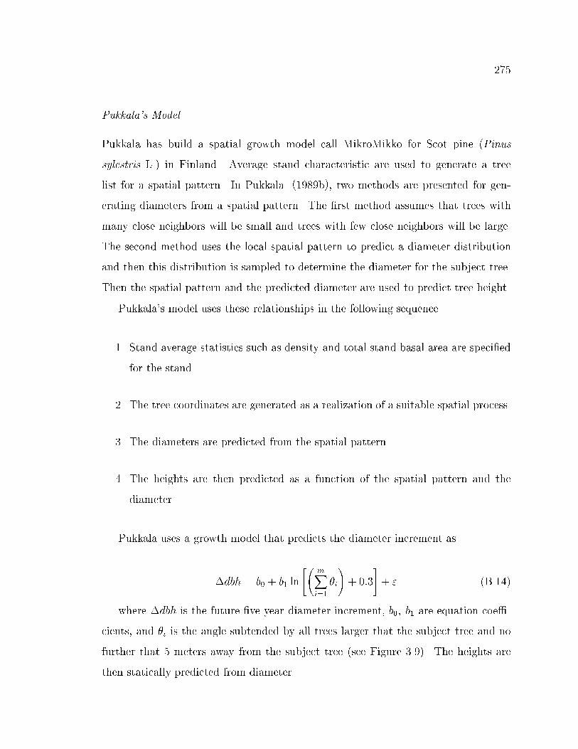
275

Pukkala's Model

Pukkala has build a spatial growth model call MikroMikko for Scot pine (Pinus

sylestris L.) in Finland. Average stand characteristic are used to generate a tree

list for a spatial pattern. In Pukkala (1989b), two methods are presented for gen-

erating diameters from a spatial pattern. The �rst method assumes that trees with

many close neighbors will be small and trees with few close neighbors will be large.

The second method uses the local spatial pattern to predict a diameter distribution

and then this distribution is sampled to determine the diameter for the subject tree.

Then the spatial pattern and the predicted diameter are used to predict tree height.

Pukkala's model uses these relationships in the following sequence.

1. Stand average statistics such as density and total stand basal area are speci�ed

for the stand.

2. The tree coordinates are generated as a realization of a suitable spatial process.

3. The diameters are predicted from the spatial pattern.

4. The heights are then predicted as a function of the spatial pattern and the

diameter.

Pukkala uses a growth model that predicts the diameter increment as

�dbh = b0 + b1 ln

" mXi=1

�i

!+ 0:3

#+ " (B.14)

where �dbh is the future �ve year diameter increment, b0; b1 are equation coe�-

cients, and �i is the angle subtended by all trees larger that the subject tree and no

further that 5 meters away from the subject tree (see Figure 3.9). The heights are

then statically predicted from diameter.

276

h = ch

"1:3 + d2

(a0 + a1d)2

#(B.15)

where h is the new height, ch is a correction factor to obtain a speci�ed height

estimate for the average tree, a0; a1 are equation coe�cients, and d is the newly

predicted diameter.

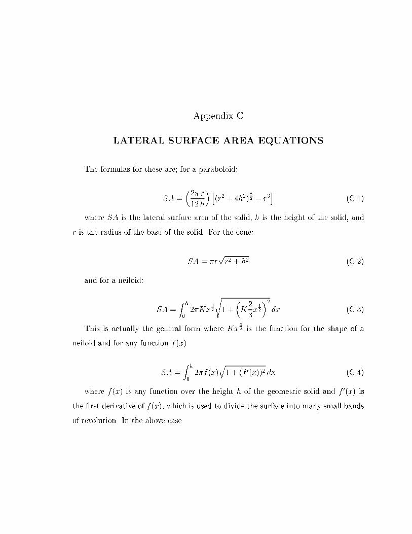
Appendix C

LATERAL SURFACE AREA EQUATIONS

The formulas for these are; for a paraboloid:

SA =�2� r

12 h

� h(r2 + 4h2)

3

2 � r3i

(C.1)

where SA is the lateral surface area of the solid, h is the height of the solid, and

r is the radius of the base of the solid. For the cone:

SA = �rpr2 + h2 (C.2)

and for a neiloid:

SA =Z h

02�Kx

3

2

s1 +

�K2

3x

1

2

�2dx (C.3)

This is actually the general form where Kx3

2 is the function for the shape of a

neiloid and for any function f(x)

SA =Z h

02�f(x)

q1 + (f 0(x))2 dx (C.4)

where f(x) is any function over the height h of the geometric solid and f 0(x) is

the �rst derivative of f(x), which is used to divide the surface into many small bands

of revolution. In the above case