0

SHRP2 R23 Using Existing Pavement in Place and Achieving Long Life

Project Assessment Manual

June 29, 2013

1

Project Assessment Manual Topics

Topic Page

Section 1 Introduction 3

Explanation as to why this manual was developed

How to use the manual

Assessment data categories

Overall Assessment Scheme

Section 2 Pavement Distress Survey 5

Purpose

Measurement methods

Analysis tools

Section 3 Pavement Rut Depth and Roughness 16

Purpose

Measurement methods

Analysis tools

Section 4 Nondestructive Testing via the Falling Weight Deflectometer (FWD) 21

Purpose

Measurement method

Analysis tools

Section 5 Ground Penetrating Radar (GPR) 36

Purpose

Measurement method

Analysis tools

Section 6 Pavement Cores 53

Purpose

Measurement method

Analysis tools

Section 7 Dynamic Cone Penetrometer (DCP) 54

Purpose

Measurement method

Analysis tools

Section 8 Subgrade Soil Sampling and Tests 62

Purpose

Measurement methods

Analysis tools

Section 9 Traffic Loads for Design 67

Purpose

Measurement method

Analysis tools

2

Project Assessment Manual Topics (continued)

Topic Page

Section 10 Construction Productivity and Traffic Impacts 73

Purpose

Measurement methods

Analysis tools

Section 11 Life Cycle Assessment (Environmental Accounting) 103

Purpose

Measurement methods

Analysis tools

Section 12 Miscellaneous Material Properties 117

3

Section 1 Introduction

1.1 Why This Assessment Manual?

This assessment manual was prepared to aid the process of renewing existing pavements so that long lives can be achieved. To achieve this goal a systematic collection of relevant pavement-related data is needed. Further, such data needs to be organized to maximize the usefulness in pavement decision-making process. To that end, this manual will help. The types of data collection contained in this manual range from basic information such as a distress survey to insights on traffic impacts. The last section provides information on life cycle assessments (environmental accounting). This type of assessment is receiving increasing usage and is likely to be widely applied in the future.

1.2 How to Use the Manual The use of the manual is to compliment the design tools developed by the SHRP2 R23 study. The types of data critical for making pavement-related decisions are described along with methods (analysis tools) for organizing the information for decision-making. It is not assumed that all data categories will be collected or assessed for a specific renewal project. Rather, the manual is designed as a reference document that provides information relevant to all renewal strategies considered in the SHRP2 R23 project.

1.3 Assessment Data Categories There are 10 categories of data contained in this manual. These are:

Pavement distress surveys

Pavement rut depths and roughness

Nondestructive Testing—Falling Weight Deflectometer

Ground Penetrating Radar

Pavement cores

Dynamic Cone Penetrometer

Subgrade soil sampling and tests

Traffic Loads for Design

Traffic impacts

Life cycle assessment Each data category is structured much the same, namely by (1) the purpose for collecting the data, (2) applicable standards, definitions and data organization recommendations, and (3) analysis tools.

4

1.4 Overall Assessment Scheme The overall assessment scheme performed by the user can range from rather basic information about the existing and proposed pavement structure to substantially more detailed data and analyses. The basic scheme is illustrated in Figure 1.1.

Figure 1.1 Outline of Assessment Scheme

The first three boxes (1 through 3) shown in Figure 1.1 are addressed in this assessment manual with that information being applied to the processes shown in the last two boxes (4 and 5). The types of input data include the distress types associated with the existing pavement structure, characterization of future traffic (in terms of ESALs and ADT), subgrade characterization (strength or stiffness) and more.

Identify Distress Categories

Select Renewal Pavement Type Option

Identify Pavement Type for Existing Pavement Structure

Apply Recommended Renewal Actions and Design

Collect other pavement related data and conduct analyses

1

2

3

4

5

5

Section 2 Pavement Distress Survey

2.1 Purpose

This section overviews the use of a pavement distress survey for aiding pavement assessment decisions.

2.2 Measurement Methods

This subsection is used to describe definitions and standards applicable for pavement distresses and provides a way to organize such information. (i) Pavement Distress Measurements: ASTM D6433-07 Standard Practice for Roads and Parking Lots Pavement Condition Index Surveys. (ii) Distress Identification Manual for the Long-Term Pavement Performance Program: FHWA-RD-03-031, June 2003.

(iii) Discussion

Pavement distress data can be used for numerous purposes but three are noted: (1) establish pavement reconstruction, rehabilitation, and maintenance priorities, (2) determine rehabilitation and maintenance strategies, and (3) predict pavement performance. This type of information is a key element for decision-making associated with pavement renewal options. McCullough (1971) provided a detailed description of three basic pavement distress groups, associated modes, and examples as shown in Table 2.1. Most all distress survey schemes use a subset of fracture, distortion, and/or disintegration. Upon closer inspection of Table 2.1 for flexible pavements, two of these—fracture and disintegration are responsible for most pavement rehabilitation and maintenance actions. More specifically these can be categorized by fatigue, transverse cracking, and stripping/raveling. Tables 2.2, 2.3, and 2.4 provide templates for flexible pavement distress data collection. It is assumed that cores will be an integral part of the pavement distress examination hence locations would logically be organized by mileposts or other appropriate location referencing system. For multilane highways, this information can be collected for the design lane or all lanes in one direction—as per project requirements.

6

Table 2.1 Distress Groups (after McCullough, 1971)

Distress Group Distress Mode Examples of Distress Mechanism

Fracture Cracking Excessive loading

Repeated loading (i.e., fatigue)

Thermal changes

Moisture changes

Slippage (horizontal forces)

Shrinkage

Spalling Excessive loading

Repeated loading (i.e., fatigue)

Thermal changes

Moisture changes

Distortion Permanent Deformation

Excessive loading

Time-dependent deformation (e.g., creep)

Densification (i.e., compaction)

Consolidation

Swelling

Frost

Faulting Excessive loading

Densification (i.e., compaction)

Consolidation

Swelling

Disintegration Stripping Adhesion (i.e. loss of bond)

Chemical reactivity

Abrasion by traffic

Raveling and Scaling

Adhesion (i.e. loss of bond)

Chemical reactivity

Abrasion by traffic

Degradation of aggregate

Durability of binder

7

The following distress types should be measured and recorded if present on the existing pavement: Flexible Pavement Distress (definitions from or modified after LTPP Distress Manual, Miller and Dellinger, 2003):

1. Fatigue cracking: Occurs in areas subjected to repeated traffic loadings (wheel paths). Can be a series of interconnected cracks in early stages of development. Develops into many-sided, sharp-angled pieces, usually less than 0.3 m on the longest side, characteristically with a chicken wire/alligator pattern, in later stages. 2. Transverse cracking: Cracks that are predominantly perpendicular to the pavement centerline. 3. Stripping or raveling: Wearing away of the pavement surface caused by the dislodging of aggregate particles and loss of asphalt binder. Raveling ranges from loss of fines to loss of some coarse aggregate and ultimately to a very rough and pitted surface with obvious loss of aggregate. This study expands the definition to identification of stripping/raveling in the surface layer to include stripping that may be occurring in lower HMA layers in the pavement structure.

Rigid Pavement Distress for JPCP, JRCP, and CRCP (definitions from or modified after LTPP Distress Manual, Miller and Dellinger, 2003 with the exception of ASR cracking):

1. Pavement Cracking: Pavement cracking includes all major types of cracks that can occur in a slab. This can include corner breaks, longitudinal and transverse cracking as defined by Miller and Dellinger, 2003. Corner break cracks intersect the adjacent transverse and longitudinal joints at approximately a 45° angle. Longitudinal and transverse cracking are parallel and transverse to the centerline, respectfully. 2. Joint Faulting: Joint faulting is the difference in elevation across a joint or crack. 3. Materials Caused Distress: (1) D-Cracking: Closely spaced crescent-shaped hairline cracking pattern; occurs adjacent to joints, cracks, or free edges; dark coloring of the cracking pattern and surrounding area; sometimes referred to as durability cracking, and (2) Alkali-Silica Reactivity (ASR) Cracking: Cracking of the PCC which can be easily confused with D-cracking or shrinkage cracking. 4. Pumping: Pumping is the ejection of water from beneath the pavement. In some cases, detectable deposits of fine material are left on the pavement surface, which were eroded (pumped) form the support layers and have stained the surface. 5. Punchouts: The area enclosed by two closely spaced (usually < 0.6 m) transverse cracks, a short longitudinal crack, and the edge of the pavement or a longitudinal joint. Also includes “Y” cracks that exhibit spalling, breakup, or faulting.

2.2.1 Pavement Distress Data Templates

The templates for specific pavement distress types follow.

8

Table 2.2 Template for Flexible Pavement Distress—Fatigue Cracking

Location (milepost)

Depth Distress

HMA (in)

Base (in)

Fatigue Cracking

Severity2 Extent1 Depth of Fatigue Cracks4 (measured from the pavement

surface)

Low

Moderate

High Notes:

1. Extent of fatigue cracking is based on % of wheelpath areas. 2. Severity of fatigue cracking is low, medium, and high. (1) Low = None or only a few connecting cracks; cracks are not spalled or sealed; pumping not evident, (2) Moderate = Interconnected cracks forming a complete pattern; cracks may be slightly spalled; cracks may be sealed; pumping is not evident, and (3) High = Moderately or severely spalled interconnected cracks forming a complete pattern; pieces may move when subjected to traffic; cracks may be sealed; pumping may be evident. The severity definitions are from the LTPP Distress Identification Manual (Miller and Bellinger, 2003). 3. Record extent for each level of severity. 4. Depth of fatigue cracks can be full depth or top down cracking. This should be determined by the use of pavement cores.

Figure 2.1 Illustrations of Fatigue Cracking Severity Levels

Low Severity (Source: Pavement Interactive)

Moderate Severity (Source: N. Jackson)

High Severity (Source: Pavement Interactive)

9

Table 2.3 Template for Flexible Pavement Distress—Transverse Cracking

Location (milepost)

Depth Distress

HMA (in)

Base (in)

Transverse Cracking

Severity2 Extent1 Depth of Transverse Cracks (measured from the pavement

surface)

Low

Moderate

High Notes:

1. Extent of transverse cracking is based on the number of cracks per 100 ft. 2. Severity of transverse cracking is low, medium, and high. (1) Low = Unsealed cracks with a mean width ≤ 6 mm; sealed cracks with sealant material in good condition and with a width that cannot be determined, (2) Moderate =

Cracks with mean widths 6 mm and ≤ 19 mm; or any cracks with a mean width ≤ 19 mm and adjacent low severity

random cracking, and (3) High = Cracks with a mean width of 19 mm; or cracks with a mean width ≤ 19 mm and adjacent to moderate to high severity random cracking. The severity definitions are from the LTPP Distress Identification Manual (Miller and Bellinger, 2003). 3. Record extent for each level of severity. 4. Depth of fatigue cracks might be full depth of the HMA or top down cracking. This can only be determined by the use of pavement cores.

Figure 2.2 Illustrations of Transverse Cracking Severity Levels

Moderate Severity (Source: Pavement Interactive)

Moderate to High Severity (Source: WSDOT)

High Severity (Source: Pavement Interactive)

10

Table 2.4 Template for Flexible Pavement Distress—Stripping/Raveling

Location (milepost)

Depth Distress

HMA (in)

Base (in)

Stripping/Raveling

Extent (% of surface area)

Full depth stripping/raveling or confined to the wearing surface only? Observation must be based on cores.

Note: Severity levels are not applicable for stripping. Either it exists or does not.

Figure 2.3 Illustration of Raveling

Using Table 2.1 again, the most important Jointed Plain Concrete Pavement (JPCP) distress types which initiates PCCP renewal actions are fracture (slab or pavement cracking), distortion (faulting—typically at transverse contraction joints), and disintegration which includes materials caused distresses of D-cracking and ASR cracking. These are shown in Tables 2.5, 2.6, 2.7, and 2.8. Tables 2.9 and 2.10 apply to CRCP and composite pavements.

Table 2.5 Template for Rigid Pavement Distress—JPCP or JRCP—Pavement Cracking

Location (milepost)

Depth Distress

PCC Slab (in)

Base Pavement or Slab Cracking

Type1 Thick (in) % Slabs with Multiple Cracks2

Comments

Notes 1. Three types of base underlying PCC: (1) Granular Base, (2) Cement Treated Base, or (3) Asphalt Treated Base.

Photo source: WSDOT

11

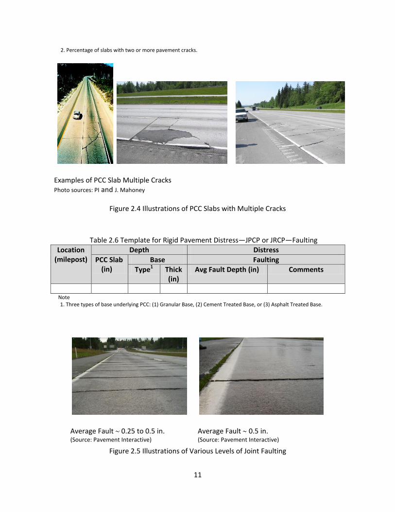
2. Percentage of slabs with two or more pavement cracks.

Figure 2.4 Illustrations of PCC Slabs with Multiple Cracks

Table 2.6 Template for Rigid Pavement Distress—JPCP or JRCP—Faulting

Location (milepost)

Depth Distress

PCC Slab (in)

Base Faulting

Type1 Thick (in)

Avg Fault Depth (in) Comments

Note 1. Three types of base underlying PCC: (1) Granular Base, (2) Cement Treated Base, or (3) Asphalt Treated Base.

Figure 2.5 Illustrations of Various Levels of Joint Faulting

Examples of PCC Slab Multiple Cracks

Photo sources: PI and J. Mahoney

Average Fault 0.25 to 0.5 in. (Source: Pavement Interactive)

Average Fault 0.5 in. (Source: Pavement Interactive)

12

Table 2.7 Template for Rigid Pavement Distress—D-Cracking

Location (milepost)

Depth Distress

PCC Slab (in)

Base D-Cracking

Type1 Thick (in) Severity2 Extent3 Comments

Low

Moderate

High Notes 1. Three types of base underlying PCC: (1) Granular Base, (2) Cement Treated Base, or (3) Asphalt Treated Base. 2. Severity of D-cracking is low, medium (moderate), and high. (1) Low = D-cracks are tight, with no loose or missing pieces, and no patching is in the affected area, (2) Moderate = D-cracks are well-defined, and some small pieces are loose or have been displaced, and (3) High = D-cracking has a well-developed pattern, with a significant amount of loose or missing material. Displaced pieces, up to 0.1 m

2, may have been patched.

3. Extent is based on the amount of cracks or joints that exhibit D-cracking. This definition of extent is different than used by LTPP.

Figure 2.6 Illustrations of D-Cracking Severity Levels

Low Severity (Source: PI and C.L. Monismith)

Low Severity (Source: N. Jackson)

High Severity (Source: N. Jackson)

13

Table 2.8 Template for Rigid Pavement Distress—ASR Cracking

Location (milepost)

Depth Distress

PCC Slab (in)

Base ASR Related Cracking

Type1 Thick (in) Does ASR Cracking Apply to this Pavement?

Yes or No

How was ASR detected or measured?

Note 1. Three types of base underlying PCC: (1) Granular Base, (2) Cement Treated Base, or (3) Asphalt Treated Base.

Figure 2.7 Illustrations of ASR Cracking Severity Levels Table 2.9 applies to Continuously Reinforced Concrete Pavement (CRCP). A critical distress for CRCP is punchouts (which falls under “fracture” in Table 2.1).

Table 2.9 Template for Rigid Pavement Distress—CRCP—Punchouts

Location (milepost)

Depth Distress

PCC Slab (in)

Base Punchouts

Type1 Thick (in) No./mile Comments

Note 1: Three types of base underlying PCC: (1) Granular Base, (2) Cement Treated Base, or (3) Asphalt Treated Base.

Early State of Cracking (Source: N. Jackson)

Advanced Stage of Cracking (Source: N. Jackson)

14

Figure 2.8 Illustration of a CRCP Punchout

Table 2.10 Composite Pavement Distress1

Location (milepost)

Depth Distress4

HMA Surfacing

(in)

PCC Describe condition of

surface course

Comments

PCC Type2

PCC Slab Thick (in.)

Base Type3

Base Thick (in)

Poor Condition

Very Poor Condition

Notes: 1. Composite pavement definition assumes a flexible (HMA) layer overlies PCC.

2. Three types of PCC pavement: (1) JPCP, (2) JRCP, or (3) CRCP. 3. Three types of base underlying PCC: (1) Granular Base, (2) Cement Treated Base, or (3) Asphalt Treated Base. 4. Distress is broadly defined for composite pavements. The only initial information available to the user is the surface condition which can include a range of distress types—most likely cracking.

Other PCCP distress types can be important and such information collected and used; however, the distress types in the preceding tables were judged as the most critical for pavement renewal decision-making.

2.2.2 Drainage Conditions An assessment of the existing pavement’s subsurface drainage is important in making pavement renewal decisions. The following factors, if observed, suggest that subsurface drainage may be an issue and corrective actions needed for the renewal design process:

Pumping

PCC joint or crack faulting

Standing water in shallow ditches

Use of cement stabilized base under PCC.

Advanced Stage for a Punchout (Source: PI and FHWA)

15

2.3 Analysis Tools

How pavement distress data is specifically used in the renewal decision-making process is covered in a separate project report.

2.4 References McCullough, B.F. (1971), "Distress Mechanisms-General," Special Report No. 126, Highway Research Board, National Academy of Sciences, Washington, DC.

Miller, J.S. and Bellinger, W.Y. (2003), “Distress Identification Manual for the Long-Term Pavement Performance Program (Fourth Edition),” Report FHWA-RD-03-031, Office of Infrastructure Research and Development, Federal Highway Administration, McLean, Virginia, June 2003.

Stark, D. (1994), “Handbook for the Identification of Alkali-Silica Reactivity in Highway Structures,” SHRP-C-315, Strategic Highway Research Program, Washington, DC, originally printed in 1994 but updated. http://leadstates.transportation.org/asr/library/C315/index.stm#f

16

Section 3

Pavement Rut Depth and Roughness (Profile)

3.1 Purpose This section overviews the use of pavement rut depths and roughness for aiding pavement assessment decisions.

3.2 Measurement Methods This subsection is used to describe definitions and standards applicable for pavement rut and roughness measurements.

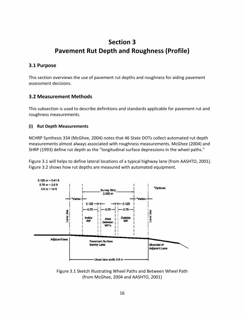
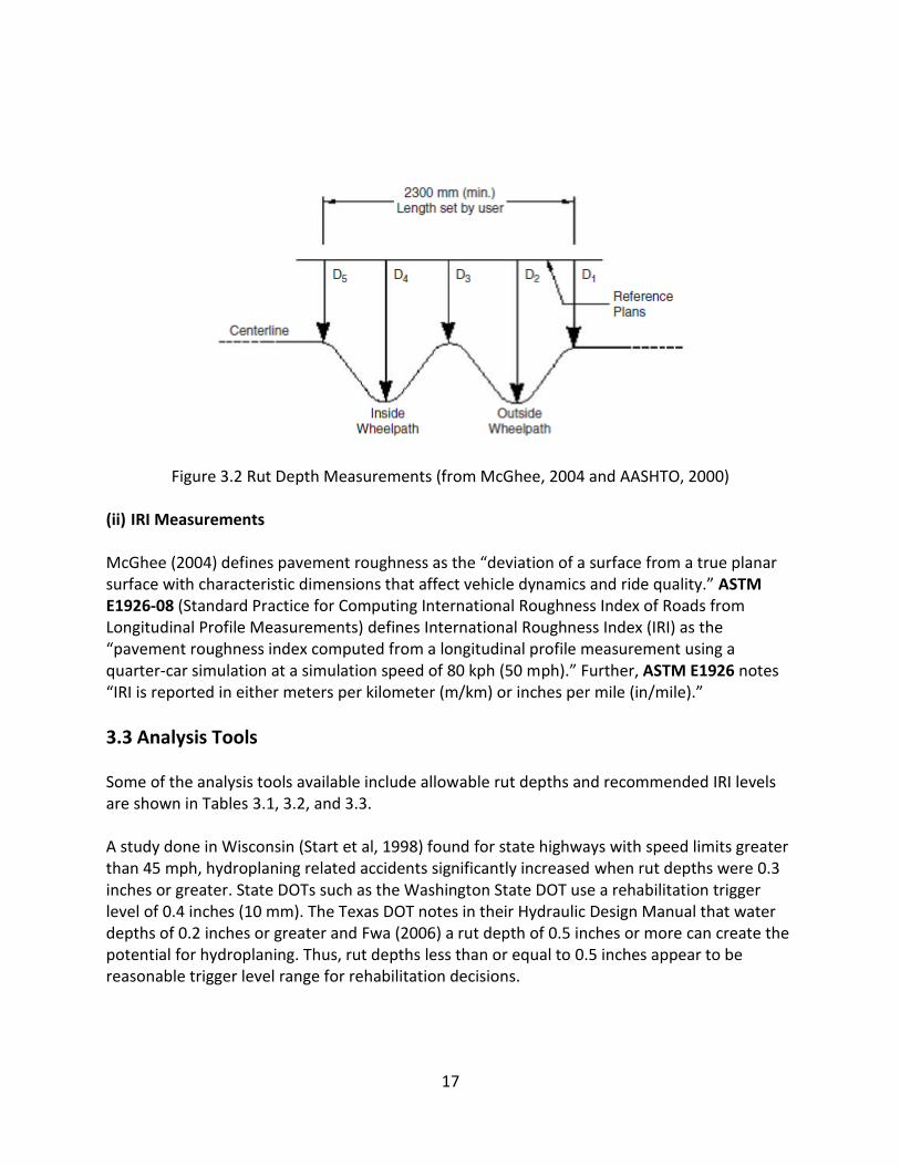
(i) Rut Depth Measurements NCHRP Synthesis 334 (McGhee, 2004) notes that 46 State DOTs collect automated rut depth measurements almost always associated with roughness measurements. McGhee (2004) and SHRP (1993) define rut depth as the “longitudinal surface depressions in the wheel paths.” Figure 3.1 will helps to define lateral locations of a typical highway lane (from AASHTO, 2001). Figure 3.2 shows how rut depths are measured with automated equipment.

Figure 3.1 Sketch Illustrating Wheel Paths and Between Wheel Path (from McGhee, 2004 and AASHTO, 2001)

17

Figure 3.2 Rut Depth Measurements (from McGhee, 2004 and AASHTO, 2000) (ii) IRI Measurements McGhee (2004) defines pavement roughness as the “deviation of a surface from a true planar surface with characteristic dimensions that affect vehicle dynamics and ride quality.” ASTM E1926-08 (Standard Practice for Computing International Roughness Index of Roads from Longitudinal Profile Measurements) defines International Roughness Index (IRI) as the “pavement roughness index computed from a longitudinal profile measurement using a quarter-car simulation at a simulation speed of 80 kph (50 mph).” Further, ASTM E1926 notes “IRI is reported in either meters per kilometer (m/km) or inches per mile (in/mile).”

3.3 Analysis Tools

Some of the analysis tools available include allowable rut depths and recommended IRI levels are shown in Tables 3.1, 3.2, and 3.3. A study done in Wisconsin (Start et al, 1998) found for state highways with speed limits greater than 45 mph, hydroplaning related accidents significantly increased when rut depths were 0.3 inches or greater. State DOTs such as the Washington State DOT use a rehabilitation trigger level of 0.4 inches (10 mm). The Texas DOT notes in their Hydraulic Design Manual that water depths of 0.2 inches or greater and Fwa (2006) a rut depth of 0.5 inches or more can create the potential for hydroplaning. Thus, rut depths less than or equal to 0.5 inches appear to be reasonable trigger level range for rehabilitation decisions.

18

Table 3.1 Typical Maximum Rut Depths

Table 3.2 FHWA IRI Criteria (from FHWA, 2006)

Ride Quality Terms

All Functional Classifications

IRI, inches/mi (m/km)

PSR Rating

Good < 95 (< 1.5)

Good

Acceptable ≤ 170 (≤ 2.7)

Acceptable

Not Acceptable > 170 (> 2.7)

Not Acceptable

Pavement Type Maximum Rut Depth, inches (mm)

Texas DOT [concern about hydroplaning]

0.2 (5)

Wisconsin Hydroplaning Study (Start et al, 1998)

0.3 (7.6)

Washington State DOT 0.4 (10)

Fwa (2006) [based on hydroplaning]

0.5 (12.5)

Shahin (1997) [from the PAVER Asphalt Distress Manual—Pavement Distress Identification Guide for Asphalt-Surfaced Roads and Parking Lots]

Low 0.25 to 0.5 (6 to 13)

Medium 0.5 to 1.0 (13 to 25)

High 1.0

( 25)

19

Table 3.3 Earlier FHWA IRI Criteria (FHWA, 1999)

Ride Quality Terms

PSR Rating IRI, in/mile (m/km)

National Highway System Ride

Quality

Very Good 4.0 60

( 0.95)

Acceptable between 0 and

170 in./mile

Good 3.5 to 3.9 60 to 94 (0.95 to 1.48)

Fair 3.1 to 3.4 95 to 119 (1.50 to 1.88)

Mediocre 2.6 to 3.0 120 to 170 (1.89 to 2.68)

Poor 2.5 170

( 2.68)

Less than acceptable

170 in./mile

The IRI criteria used by the FHWA have evolved as illustrated by review of Tables 3.2 and 3.3. In 1999, the most detailed breakdown, suggests that IRI values of less than 60 inches/mile are quite good and greater than 170 inches/mile poor. Interestingly, many newly paved HMA projects typically have IRI values close to the 60 inches/mile value. Eventually, the FHWA simplified their criteria as shown in Table 3.2. A study conducted on Seattle area urban freeways using driver in-vehicle opinion surveys (Shafizadeh and Mannering, 2003) confirmed that motorists find pavements with IRI values less than 170 inches/mile acceptable as to ride quality (85% acceptable). The paper concluded that that there was no evidence to change federal IRI guides (in essence those shown in Table 3.3).

3.4 References AASHTO (2000), “Standard Practice for Determining Maximum Rut Depth in Asphalt Pavements,” AASHTO Designation PP38-00, American Association of State Highway and Transportation Officials. AASHTO (2001), “Standard Practice for Quantifying Cracks in Asphalt Pavement Surfaces,” AASHTO Designation PP44-01, American Association of State Highway and Transportation Officials, April 2001. FHWA (1999), “1999 Status of the Nation’s Highways, bridges, and Transit: Conditions and Performance,” Report FHWA-PL-99-017, Federal Highway Administration, November 1999. FHWA (2006), “2006 Status of the Nation’s Highways, Bridges, and Transit: Conditions and Performance,” Federal Highway Administration, http://www.fhwa.dot.gov/policy/2006cpr/chap3.htm

20

Fwa, T. (2006), The Handbook of Highway Engineering, Taylor and Francis Group, CRC Press. McGhee, K. (2004), “Automated Pavement Distress Collection Techniques,” Synthesis 334, National Cooperative Highway Research Program, Transportation Research Board. Shafizadeh, K. and Mannering, F. (2003), “Acceptability of Pavement Roughness on Urban Highways by Driving Public,” Transportation Research Record 1860, Transportation Research Board. Shahin, M. (1997), “PAVER Distress Manual,” TR 97/104, US Army Construction Engineering Research Laboratories, Champaign, IL, June 1997. Start, M., Jeong, K., and Berg, W. (1998), “Potential Safety Cost-Effectiveness of Treating Rutted Pavements, Transportation Research Record 1629, Transportation Research Board. SHRP (1993), “Distress Identification Manual for the Long-Term Pavement Performance Project,” Strategic Highway Research Program, National Research Council. Texas DOT (2009), “Hydroplaning,” Hydraulic Design Manual, Texas DOT, March 1, 2009.

21

Section 4 Nondestructive Testing via the Falling Weight Deflectometer

4.1 Purpose This section overviews the most commonly used Falling Weight Deflectometer (FWD) in use and how it can be used to aid pavement assessment decisions.

4.2 Measurement Method This subsection will briefly overview impact (or impulse) pavement loading. The device described is the Dynatest FWD. This device can obtain measurements rapidly and the impact load is easily varied.

All impact load NDT devices deliver a transient impulse load to the pavement surface. The subsequent pavement response (deflection) is measured. Standard test methods include:

(i) ASTM D4694-96: Standard Test Method for Deflections with a Falling-Weight-Type Impulse Load Device

(ii) ASTM D4695-03: Standard Guide for General Pavement Deflection Measurements

The significant features of ASTM D4694 include: (1) the force pulse will approximate a haversine or half-sine wave, (2) the peak force of 11,000 lb must be achievable by the loading device, (3) the force-pulse duration should be within range of 20 to 60 ms with a rise time in range of 10 to 30 ms, (4) the loading plates standard sizes are 300 mm (12 in.) and 450 mm (18 in.), (5) the deflection transducers, which are used to measure the maximum vertical movement of the pavement, can be seismometers, velocity transducers, or accelerometers, (6) the load measurements must be accurate to at least ± 2 percent or ± 160 N (± 36 lb), whichever is greater, (7) the deflection measurements must be accurate to at least ± 2 percent or ± 2 µm (± 0.08 mils), whichever is greater. Note that 0.08 mils = 0.00008 inch and 2 µm = 0.002 mm, and (8) a precision guide in ASTM D4694 notes when a device is operated by a single operator in repetitive tests at the same location, the test results are questionable if the difference in the measured center deflection (D0) between two consecutive tests at the same drop height (or

force level) is greater than 5 percent. For example, if D0 = 0.254 mm (10 mils) then the next

load must result in a D0 range less than 0.241 mm to 0.267 mm (9.5 to 10.5 mils).

22

(iii) Dynatest FWD

The Dynatest FWD is the most widely used FWD in the US. The device is trailer mounted and uses deflection sensors that are velocity transducers. By use of different drop weights and heights this device can vary the impulse load to the pavement structure from about 1,500 to 27,000 lb. The weights are dropped onto a rubber buffer system resulting in a load pulse of 0.025 to 0.030 seconds. The standard load plate has a 300 mm (11.8 in.) diameter.

Locations for the seven velocity transducers vary. From ASTM D4694 “the number and spacing of the sensors is optional and will depend upon the purpose of the test and the pavement layer characteristics. A sensor spacing of 12 in. is frequently used. A number of State DOTs have used:

The Strategic Highway Research Program (SHRP) sensor spacing with the 11.8 in. load plate are:

Distance from the center of the load

plate (in.)

0

8

12

24

36

48

Distance from the center of the load

plate (in.)

0

8

12

18

24

36

60

23

4.3 Analysis Tools

This subsection will focus on straightforward analysis tools that can be applied to FWD deflection results.

4.3.1 Description of Available Analysis Tools for Flexible Pavements

This subsection will be used to describe three data assessment tools: (1) maximum deflection, (2) the Area Parameter, and (3) a simplified method for calculating subgrade modulus.

The use of selected indices and algorithms provide a "picture" of the relative conditions found throughout a project. This picture is useful in performing backcalculation and may at times be used by themselves on projects with large variations in surfacing layers. Deflections measured at the center of the test load combined with Area values and ESG computed from deflections

measured at 24 in. from the center of the load plate are shown in the linear plot to provide a visual picture of the conditions found along the length of any project (as illustrated by data from a rural road in Figure 4.1).

Figure 4.1 Illustrations of FWD Deflection Data Summarized by the Three Types of Data

24

The deflection data in Figure 4.1 is “normalized” data in that the measured deflections are calculated for a 9,000 lb load. The modulus determination was based on the deflection 24 in. from the center of the load plate. Table 4.1 provides general information about conclusions that can be drawn from the FWD parameters of Area and D0.

Table 4.1 General Information about the Area and D0

FWD Based Parameter Generalized Conclusions*

Area Maximum Surface Deflection (D0)

Low Low Weak structure, strong subgrade

Low High Weak structure, weak subgrade

High Low Strong structure, strong subgrade

High High Strong structure, weak subgrade

(i) Maximum pavement deflection (D0)

The maximum pavement deflection can vary widely for different pavement structures and throughout the day as its temperature changes. D0 ranges can be grouped into the following broad and approximate categories (Table 4.2):

Table 4.2 D0 Ranges

(ii) Area Parameter

The Area Parameter represents the normalized area of a slice taken through any deflection basin between the center of the test load and 3 ft. By normalized, it is meant that the area of the slice is divided by the deflection measured at the center of the test load, D0. Thus the Area

Parameter is the length of one side of a rectangle where the other side of the rectangle is D0;

hence, the Area Parameter has units of inches.

Maximum Surface Deflection (D0) Level

Generalized Conclusions

Approximate D0 (in.)

Low Deflections Strong structure 0.020

Medium Deflections Medium structure 0.030

High Deflections Weak structure 0.050

25

The Area equation is:

A = 6(D0 + 2D1 + 2D2 + D3)/D0

where D0 = surface deflection at center of test load,

D1 = surface deflection at 1 ft,

D2 = surface deflection at 2 ft, and

D3 = surface deflection at 3 ft.

The maximum value for Area is 36.0 and occurs when all four deflection measurements are equal (not likely to actually occur) as follows: If, D0 = D1 = D2 = D3 then, Area = 6(1 + 2 + 2 + 1) = 36.0 in.

For all four deflection measurements to be equal (or nearly equal) would indicate an extremely stiff pavement system (like portland cement concrete slabs or thick, full-depth asphalt concrete.) The minimum Area value should be no less than 11.1 in. This value can be calculated for a one-layer system which is analogous to testing (or deflecting) the top of the subgrade (i.e., no pavement structure). Using appropriate equations, the ratios of

D1D0

, D2D0

, D3D0

always result in 0.26, 0.125, and 0.083, respectively. Putting these ratios in the Area equation results in Area = 6(1+ 2(0.26) + 2(0.125) + 0.083) = 11.1 in. Further, this value of Area suggests that the elastic moduli of any pavement system would all be equal (e.g., E1 = E2 = E3 = …). This

is highly unlikely for actual, in-service pavement structures. Low area values suggest that the pavement structure is not much different from the underlying subgrade material (this is not always a bad thing if the subgrade is extremely stiff). Typical Area values are shown in the Table 4.3.

Table 4.3 Typical Area Values

Pavement Structure Area Parameter (in.)

PCCP Range 24-33

“Sound” PCC 29-32

Thick HMA ( 9 in. of HMA) 27+

Medium HMA ( 5 in. of HMA) 23

Thin HMA ( 2 in. of HMA) 17

Chip sealed flexible pavement 15-17

Weak chip sealed flexible pavement 12-15

26

(iii) Subgrade Modulus

An NCHRP study [Darter, et al, 1991] which revised Part III of the AASHTO Pavement Guide recommended that the following equation be used to solve for subgrade modulus:

MR = P(1 - µ2)/( )(Dr)(r) (Eq. 4.1)

where MR = backcalculated subgrade resilient modulus (psi),

P = applied load (lbs) from the FWD,

Dr = pavement surface deflection a distance r from the center of the load plate (inches), and

r = distance from center of load plate to Dr (inches). Using a Poisson's ratio of 0.40, Equation 4.1 reduces to

MR = 0.01114 (P/D2) (Eq. 4.2)

MR = 0.00743 (P/D3) (Eq. 4.3)

MR = 0.00557 (P/D4) (Eq. 4.4)

for sensor spacing of 2 ft (610 mm), 3 ft (914 mm), and 4 ft (1219 mm). If a Poisson's ratio of 0.45 is used instead for the same sensor spacing, the equations become:

MR = 0.01058(P/D2) (Eq. 4.5)

MR = 0.00705 (P/D3) (Eq. 4.6)

MR = 0.00529 (P/D4) (Eq. 4.7) Darter et al (1991) recommended that the deflection used for subgrade modulus determination should be taken at a distance at least 0.7 times r/ae where r is the radial distance to the

deflection sensor and ae is the radial dimension of the applied stress bulb at the subgrade

"surface." The ae dimension can be determined from the following:

ae = a2 + D 3 EP

MR

2

where ae = radius of stress bulb at the subgrade-pavement interface,

a = NDT load plate radius (inches),

D = total thickness of pavement layers (inches)

EP = effective pavement modulus (psi), and

27

MR = backcalculated subgrade resilient modulus.

For "thin" pavements, ae ~– 15 in. and "medium" to "thick" pavements, ae ~– 26 to 33 in. Thus, the minimum r is usually 24 to 36 in. (recall r > 0.7 (ae)).

Typical subgrade moduli are shown in the Table 4.4 below (after Chou et al, 1989):

Table 4.4 Typical Subgrade Moduli

Material Subgrade Moduli and Climate Condition

Dry, psi Wet — No Freeze, psi

Wet - Freeze

Unfrozen, psi Frozen, psi

Clay 15,000 6,000 6,000 50,000 Silt 15,000 10,000 5,000 50,000 Silty or Clayey Sand

20,000 10,000 5,000 50,000

Sand 25,000 25,000 25,000 50,000 Silty or Clayey Gravel

40,000 30,000 20,000 50,000

Gravel 50,000 50,000 40,000 50,000

4.3.2 Examples of Analyses of FWD deflection basins for Flexible Pavement The following deflection basins shown in Table 4.5 were obtained with a Dynatest FWD. The

pavement temperature at the time of testing was 46°F (8 C). The deflection basins for the four FWD drops and normalized to 9,000 lb are shown below:

Table 4.5 Example FWD Deflection Data

FWD Load (lb)

Deflection (mils)

D0 D8” D12” D24” D36” D48”

16,987 27.07 21.55 18.60 11.27 7.33 5.28

12,070 21.28 16.98 14.62 8.67 5.56 3.98

9,406 17.53 13.95 11.98 7.01 4.45 3.23

6,186 12.33 9.77 8.31 4.65 2.88 2.05

Normalized to 9000 lb.

16.59 13.24

11.34

6.58

4.18

2.99

The pavement structure at the time of FWD testing was:

HMA: 6.0 in. and the HMA layer exhibited some fatigue cracking.

Granular Base (sandy gravel): 18.0 in.

28

Subgrade: Silt (ML) with a wide seasonal variation in water table depth. The soil is frost susceptible and this area can have substantial ground freezing. At the time of testing the spring thaw had occurred about one month earlier.

(i) Requirements

Analyze the available data to characterize the overall structure and estimate the layer properties (moduli) using only the information provided above.

(ii) Results

Maximum surface deflection The maximum surface deflection = 0.01657 in. for a pavement with 6 in. of HMA. This value suggests a “low” pavement deflection. Subgrade Modulus (closed form equations) from the AASHTO Guide (1993)

MR = P(1- 2)/( )(Dr)(r)

= 9000(1-0.452)/( )(0.00418) (36)

15,200 psi

Check r 0.7(ae), OK.

The pavement subgrade modulus for a ML silt is better than average.

Area Parameter

Area = 6(D0 + 2D12” + 2D24” +D36”)/D0 = 6(0.01659 + (2)(0.01134) + (2)(0.00658) + 0.00418)/0.01659

20.5 in.

This Area Parameter is low for this thickness of AC. Thus, the Area value suggests a weak pavement structure but not extremely so.

(iii) Detailed Project Data Example

Table 4.6 below summarizes deflection data that was collected on a portion of an actual project. The project was about 5 miles in length and FWD testing was performed every 250 feet but only four of FWD locations are shown (these locations were also coring sites). The

average pavement temperature at the time the FWD data was collected was 46 F to 50 F. The timing of the survey was about 1.5 to 2 months after the spring thaw in this area.

29

As shown in the Table 4.6, the normalized D0 deflections range from about 9 to 36 mils. Deflections less than about 30 mils are considered normal. The HMA thicknesses varied between 4.6 to 5.3 inches with an average of 5.2 inches which constitutes a “medium” thickness of HMA (refer back to Table 4.2).

The Area values shown in the table suggest weak HMA, but not necessarily extreme weakness due to stripping. Table 4.7 illustrates typical theoretical Area values for various uncracked HMA thicknesses which aids this type of comparison.

Table 4.6 FWD Deflections, Area Value, and Subgrade Modulus

Core Location (MP)

Load (lbf)

Deflections (mils) Area Value

(in)

MR (psi)

D0 D8 D12 D24 D36 D48

207.85 16,940 31.30 26.18 23.19 13.78 9.09 6.65

12,086 24.21 20.31 18.11 10.35 6.81 4.96

9,421 19.45 16.38 14.57 8.11 5.28 3.98

6,218 13.19 11.26 9.92 5.12 3.39 2.83

Normalized Values 18.39 15.51 13.78 7.60 5.00 3.82 21 14,358

208.00 16,987 27.04 21.53 18.58 11.26 7.32 5.28

12,070 21.26 16.97 14.61 8.66 5.55 3.98

9.405 17.52 13.94 11.97 7.01 4.45 3.23

6,186 12.32 9.76 8.31 4.65 2.87 2.05

Normalized Values 16.57 13.23 11.34 6.57 4.17 2.99 20 16,534

208.50 16,829 14.92 11.89 10.23 5.91 3.19 2.28

12,245 11.65 9.29 7.95 4.49 2.13 1.73

9,533 9.61 7.63 6.53 3.62 1.81 1.30

6,297 6.73 5.35 4.49 2.40 1.26 0.87

Normalized Values 9.01 7.17 6.10 3.39 1.69 1.26 19 32,198

209.00 16,305 59.25 48.58 42.52 21.30 9.53 5.12

11,737 46.14 37.52 32.56 15.59 6.69 3.58

9,247 36.93 29.80 25.63 11.77 4.96 2.68

6,154 25.00 19.88 16.77 7.28 3.03 1.73

Normalized Values 35.51 28.66 24.61 11.42 4.84 2.64 19 9,572

30

Table 4.7 Typical Theoretical Area Values for Uncracked HMA

HMA Thickness (in.) Approximate Area Parameter (in.)

Normal Stiffness Low Stiffness 2 17 16

3 19 18

4 21 19

5 23 21

6 24 22

7 26 22

8 26 23

9 27 24

10 28 24

A quick, slightly more formal check of the pavement structure is to compare the actual Area value to see if it falls within the range (normal to low stiffness), above this range (above normal stiffness) or below this range (below normal stiffness). This comparison is shown in Table 4.8.

Table 4.8 Comparison of Area Value and Acceptable Area Value Range

4.3.3 Description of Available Analysis Tools for Rigid Pavements Rehabilitation of portland cement concrete pavements is not straightforward. To provide a more consistent analysis process, the load transfer efficiency should be checked with FWD obtained deflection data if the pavement type is jointed plain concrete pavement (JPCP). (i) Load Transfer Efficiency

When a wheel load is applied at a joint or crack, both the loaded slab and adjacent unloaded slab deflect. The amount the unloaded slab deflects is directly related to joint performance. If a joint is performing perfectly, both the loaded and unloaded slabs deflect equally.

Core Location

HMA Thickness

(in.)

Actual Area (in.)

Above, Below or Within Range

207.85 5.3 21 Within

208.00 6.0 20 Below

208.50 4.7 19 Below

209.00 4.6 19 Below

31

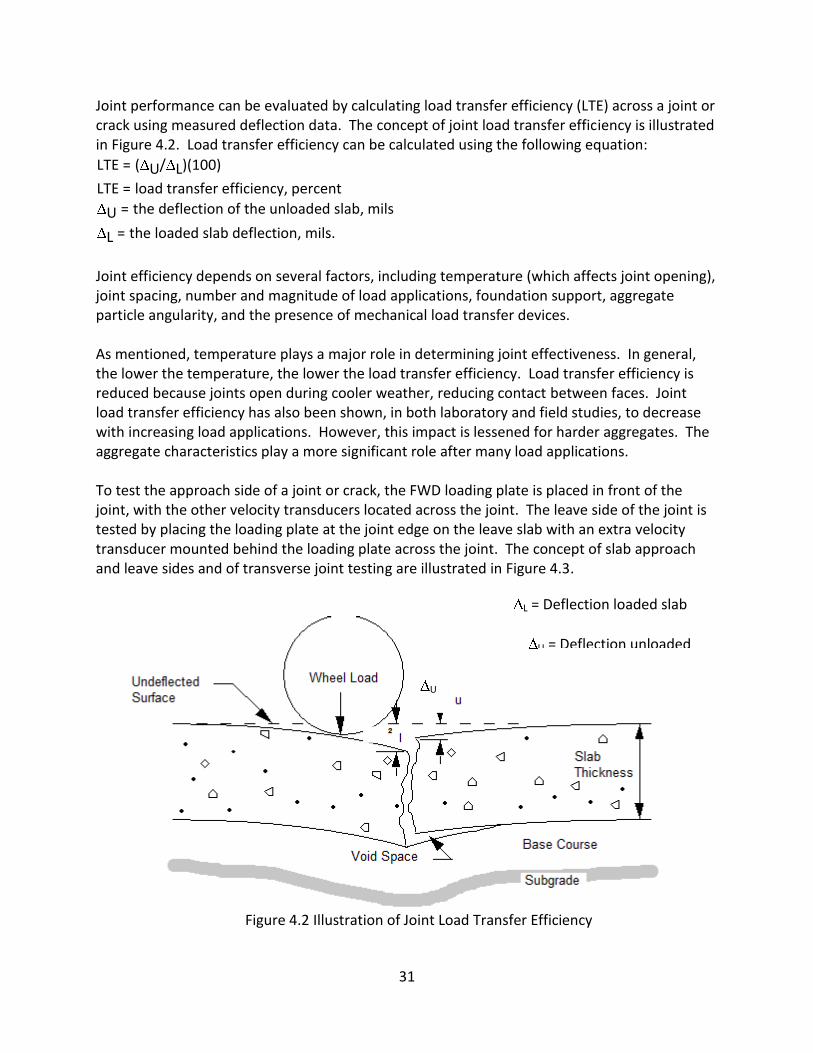
Joint performance can be evaluated by calculating load transfer efficiency (LTE) across a joint or crack using measured deflection data. The concept of joint load transfer efficiency is illustrated in Figure 4.2. Load transfer efficiency can be calculated using the following equation:

LTE = ( U/ L)(100)

LTE = load transfer efficiency, percent

U = the deflection of the unloaded slab, mils

L = the loaded slab deflection, mils.

Joint efficiency depends on several factors, including temperature (which affects joint opening), joint spacing, number and magnitude of load applications, foundation support, aggregate particle angularity, and the presence of mechanical load transfer devices. As mentioned, temperature plays a major role in determining joint effectiveness. In general, the lower the temperature, the lower the load transfer efficiency. Load transfer efficiency is reduced because joints open during cooler weather, reducing contact between faces. Joint load transfer efficiency has also been shown, in both laboratory and field studies, to decrease with increasing load applications. However, this impact is lessened for harder aggregates. The aggregate characteristics play a more significant role after many load applications. To test the approach side of a joint or crack, the FWD loading plate is placed in front of the joint, with the other velocity transducers located across the joint. The leave side of the joint is tested by placing the loading plate at the joint edge on the leave slab with an extra velocity transducer mounted behind the loading plate across the joint. The concept of slab approach and leave sides and of transverse joint testing are illustrated in Figure 4.3.

Figure 4.2 Illustration of Joint Load Transfer Efficiency

U

L

L = Deflection loaded slab

U = Deflection unloaded slab

32

Figure 4.3 Locations of FWD Load Plate and Deflection Sensors for Determining Load

Transfer Efficiency

The percentage load transfer can vary between almost 100% (excellent) to near 0% (extremely low). AASHTO (1993) notes that load transfer restoration should be considered for transverse joints and cracks with load transfer efficiencies ranging between 0 to 50%. It has been observed for numerous in-service jointed PCC pavements that load transfer efficiencies of 70% or greater generally provides good joint or crack performance.

4.3.4 Backcalculation Backcalculation is the process by which pavement layer moduli are estimated by matching measured and calculated surface deflection basins. This is done via a computer program and there are a number of these available in the US. It is likely that within a specific state there is a preferred backcalculation software package to use.

1 2 3 2

1

1

1 3 2

3

33

The general guidelines which follow are broad in scope and should be considered “rules-of-thumb.” (i) Number of Layers Generally, use no more than 3 or 4 layers of unknown moduli in the backcalculation process (preferably, no more than 3 layers). If a three layer system is being evaluated, and questionable results are being produced (weak or low stiffness base moduli, for example), it is sometimes advantageous to evaluate this pavement structure as a two layer system. This modification would possibly indicate that the base material has been contaminated by the underlying subgrade and is weaker due to the presence of fine material. Alternatively, a stiff layer should be considered if not done so previously (see below). If a pavement structure consists of a stiffer layer between two weak layers, it may be difficult to obtain realistic backcalculated moduli. For example, a pavement structure which consists of deteriorated asphalt concrete over a cement treated base. (ii) Thickness of Layers Surfacing. It can be difficult to “accurately” backcalculate HMA or BST moduli for bituminous surface layers less than 3 in. thick. Such backcalculation can be attempted for layers less than 3 in., but caution is suggested. In theory, it is possible to backcalculate separate layer moduli for various types of bituminous layers within a flexible pavement. Generally, it is not advisable to do this since one can quickly be attempting to backcalculate too many unknown layer moduli (i.e., greater than 3 or 4). By necessity, one should expect to combine all bituminous layers (seal coats, asphalt concrete, etc.) into “one” layer unless there is evidence (or the potential) for distress, such as stripping, in a HMA layer or some other such distress which is critical to pavement performance. Unstabilized Base/Subbase Course. “Thin” base course beneath “thick” surfacing layers (say HMA or PCC) often result in low base moduli. There are a number of reasons why this can occur. One, a thin base is not a “significant” layer under a stiff, thick layer. Second, the base modulus may be relatively “low” due to the stress sensitivity of granular materials. The use of a stiff layer generally improves the modulus estimate for base/subbase layers. (iii) Subgrade If unusually high subgrade moduli are calculated, check to see if a stiff layer is present. Stiff layers, if unaccounted for in the backcalculation process, will generally result in unrealistically high subgrade moduli. This is particularly true if a stiff layer is within a depth of about 20 to 30 feet below the pavement surface.

34

(iv) Stiff Layer Often, stiff layers are given “fixed” stiffness ranging from 100,000 to 1,000,000 psi with semi-infinite depth. This, in effect, makes the “subgrade” a layer with a “fixed” depth instead of the normally assumed semi-infinite depth. What is not so clear is whether one should always fix the depth to stiff layer at say 20, 30, or 50 feet if no stiff layer is otherwise indicated (i.e., use a semi-infinite depth for the subgrade). The depth to stiff layer should be verified whenever possible with other NDT data or borings. The stiffness (modulus) of the stiff layer can vary. If the stiff layer is due to saturated conditions (e.g. water table) then moduli of about 50,000 psi appear more appropriate. If rock or stiff glacial tills are the source of the stiff layer then moduli of about 1,000,000 psi appear to be more appropriate. (v) Layer Moduli A few comments about layer moduli are appropriate. Cracked HMA Moduli. Generally, fatigue cracked HMA (about 10 percent wheelpath cracking) is often observed to have backcalculated moduli of about 100,000 to 250,000 psi. What is most important in the backcalculation process, assuming surface fatigue cracking is present, is to determine whether the cracks are confined to only the immediate wearing course or penetrate through the whole depth of the HMA layer. For HMA layers greater than 6 in. thick, cracking only in the wearing course is often observed and the overall HMA layer will have a substantially higher stiffness than noted above (at moderate layer temperatures of say 75 to 80°F). Base and Subbase Moduli. Typical base and subbase moduli are shown in Table 4.9.

Table 4.9 Typical Unstabilized and Stabilized Base and Subbase Moduli

Material Typical Modulus (psi) Modulus Range (psi) Unstabilized

Crushed Stone or Gravel Base 35,000 10,000 to 150,000

Crushed Stone or Grave Subbase 30,000 10,000 to 100,000

Sand Base 20,000 5,000 to 80,000

Sand Subbase 15,000 5.000 to 80,000

Stabilized

Material Compressive Strength (psi)

Typical Modulus (psi)

Modulus Range (psi)

Lime Stabilized < 250 30,000 5,000 to 100,000

250 to 500 50,000 15,000 to 150,000

500 70,000 20,000 to 200,000

Cement Stabilized < 750 400,000 100,000 to 1,500,000

750 to 1250 1,000,000 200,000 to 3,000,000

1250 1,500,000 300,000 to 4,000,000

35

Subgrade Moduli. Typical subgrade moduli were previously shown in Table 4.5. (vi) Backcalculation Summary Performing backcalculation of pavement layer moduli is part science and part art; thus, experience typically will improve the estimated results. It is advisable to initially work with someone who has solid experience doing backcalculation or take a short course on the topic—assuming one is available. It will take only a few projects along with experience from others to become well informed on this powerful assessment technique.

4.4 References AASHTO (1993), “AASHTO Guide for Design of Pavement Structures, 1993,” American Association of State Highway and Transportation Officials, Washington, DC.

Chou, Y. J., Uzan, J., and Lytton, R. L., "Backcalculation of Layer Moduli from Nondestructive Pavement Deflection Data Using the Expert System Approach," Nondestructive Testing of Pavements and Backcalculation of Moduli , ASTM STP 1026, American Society for Testing and Materials, Philadelphia, 1989, pp. 341 - 354.

Darter, M.I., Elliott, R.P., and Hall, K.T., (1991) "Revision of AASHTO Pavement Overlay Design Procedure," Project 20-7/39, National Cooperative Highway Research Program, Transportation Research Board, Washington, D.C., September 1991.

36

Section 5 Ground Penetrating Radar

5.1 Purpose

This section describes Ground Penetrating Radar (GPR) technology and presents an overview of the most common applications of both air coupled and ground coupled GPR systems for aiding in pavement assessment decisions.

5.2 Measurement Method

This section briefly describes the two types of GPR and the basic principles of operation. The standard references for GPR applications in highways are: AASHTO PP 40-00 Standard Recommended Practice for Application of Ground Penetrating Radar to Highways ASTM D6087-08 Standard Test Method for Evaluating Asphalt Covered Concrete Bridge Decks using Ground Penetrating Radar ASTM D6432- 99 (2005) Standard Guide for Using Surface Ground Penetrating Radar Method for Subsurface Investigation (i) Air Coupled GPR systems

A typical commercially available 2.2 GHz air-coupled Ground Penetrating Radar unit is shown in Figure 5.1. The radar antenna is attached to a fiber glass boom and suspended about 5 feet from the vehicle and 14 inches above the pavement. This particular GPR unit can operate at highway speeds (70 mph); it transmits and receives 50 pulses per second, and can effectively penetrate to a depth of around 20 to 24 inches. All GPR systems include a distance measuring system and many of the new systems also have synchronized/integrated video logging, so the operator can view both surface and subsurface conditions. GPS is also included in many new systems for identifying problem locations The advantages of these systems are the speed data collection which does not require any special traffic control. The GPR generate clean signals which without filtering are ideal for quantitative analysis using automated data processing techniques to compute layer dielectrics and thickness. These systems are also excellent for locating near surface defects in flexible pavements. The disadvantages are a) the limit depth of penetration, b) not ideal for penetrating thick concrete pavements and c) the most popular operating frequency (1GHz) is now subject to FCC restrictions in the US.

37

Figure 5.1 Air Coupled GPR systems for highways

(ii) Ground Coupled GPR systems

As shown in Figure 5.2, a whole range of different operating frequencies are available for ground coupled GPR systems. The selection of the best frequency for a particular application depends on the required depth of penetration. As the name implies these antennas have to stay in close contact to the pavement under test. The advantage of these systems is their depth of penetration, several of the lower frequency systems can penetrate 20 feet under ideal conditions. The higher frequency systems are superior for many concrete pavement applications such as locating both reinforcing steel and sub-slab defects such as voids or trapped moisture. The disadvantage of these is the speed of data collection, when towed behind a vehicle the maximum speed is around 5 mph. The signals are also noisy and filtering is required. Substantial training is required to clean up and interpret ground coupled GPR data.

38

Figure 5.2 Ground coupled systems, 1.5 GHz on left, lower frequency antennas with control unit on right

5.3 Analysis Tools

All GPR systems send discrete pulses of radar energy into the pavement and capture the reflections from each layer interface within the structure. Radar is an electro-magnetic (e-m) wave and therefore obeys the laws governing reflection and transmission of e-m waves in layered media. At each interface within a pavement structure a part of the incident energy will be reflected and a part will be transmitted. It is normal to collect between 30 and 50 GPR return signals per second, which for high speed air coupled surveys could mean on trace for every 2 to 3 feet of travel. The captured return signal is often color coded and stacked side by side to provide a profile of subsurface conditions, this is analogous to an “X-Ray” of the pavement structure. Examples of this will be given later. However with air coupled signals as described below these signals can also be used to automatically calculate the engineering properties of the pavement layers.

5.3.1 Air Coupled GPR system

A typical plot of captured reflected energy versus time for one pulse of an air coupled GPR system is shown in Figure 5.3, as a graph of volts versus arrival time in nanoseconds. To understand GPR signals it is important to understand the significance of this plot.

39

Figure 5.3 Captured GPR reflections from a typical flexible pavement

The reflection A0 is known as the end reflection it is internally generated system noise which will be present in all captured GPR waves. The more important peaks are those that occur after A0. The reflection A1 (in volts) is the energy reflected from the surface of the pavement and A2 and A3 are reflections from the top of the base and subgrade respectively. These are all classified as positive reflections, which indicate an interface with a transition from a low to a high dielectric material (typically low to higher moisture content). These amplitudes of reflection and the time delays between reflections are used to calculate both layer dielectrics and thickness. The dielectric constant of a material is an electrical property which is most influenced by moisture content and density, it also governs the speed at which the GPR wave travels in the layer. An increase in moisture will cause an increase in layer dielectric; in contrast an increase in air void content will cause a decrease in layer dielectric. The equations to calculate surface layer thickness and dielectrics are summarized below:

2

1

1

/1

/1

m

ma

AA

AA (Eq 1)

40

where a = the dielectric of the surface layer,

A1 = the amplitude of surface reflection, in volts

Am = the amplitude of reflection from a large metal plate in volts (this represents the

100% reflection case, see Figure 5.1 for the metal plate test)

a

tcxh 1

1 (Eq 2)

where h1 = the thickness of the top layer

c = a constant speed of e-m wave in air (5.9 ins/ns two way travel)

t1 = the time delay between peaks A1 and A2, (in ns)

Similar equations are available for calculating the base layer dielectric and thickness. This calculation process is performed automatically in most operating systems with the end user simply getting a table of layer properties. In most GPR projects several thousand GPR traces like Figure 5.3 are collected. In order to conveniently display and interpret this information color-coding schemes are used to convert the traces into line scans and then stack them side-by-side so that a subsurface image of the pavement structure can be obtained. This approach is shown below in Figure 5.4.

41

Figure 5.4 Color Coding and stacking individual GPR images

The raw GPR image collection is displayed vertically in the middle of Figure 5.4. This image is for one specific location in the pavement. The GPR antenna shoots straight down and the resulting thickness and dielectric estimates are point specific. The single trace generated is color coded into a line scan using the color scheme in the middle of Figure 5.4. In the current scheme the high positive reflections are colored red and the negatives are colored blue. The green color is used where the reflections are near zero and are of little significance. These individual line scans are stacked so that a display for a length of pavement is developed. Being able to read and interpret these images is critical to effectively using GPR for pavement investigations, to locate section breaks in the pavement structure and to pinpoint the location of subsurface defects. An example of a typical GPR display for approximately 3000 ft by 24 inches deep of a thick flexible pavement is shown in Figure 5.5. This is taken from a section of newly constructed thick asphalt pavement over a thin granular base. In all such displays the x axis is distance (in miles and feet) along the section and the y axis is a depth scale in inches.

42

Figure 5.5 Color-Coded GPR Traces

The labels on this figure are as follows A) GPR files being used in analysis, B) Main Pull down menu bar, C) button to define the color coding scheme, D) Distance scale (miles and feet), E) end location of data within the GPR file (1mile and 3479 feet), G) depth scale in inches, with the zero (0) being the surface of the pavement, F) Default dielectric value used to convert the measure time scale into a depth scale. The important feature of this figure are the lines marked H, I and J these are the reflection from the surface, top and bottom of base respectively. This pavement is homogeneous and the layer interfaces are easy to detect.

When processing GPR data the first step is to develop displays such as Figure 5.5. From this it is possible to identify any clear breaks in pavement structure and to identify any significant subsurface defects. The intensity of the subsurface colors is related to the amplitude of reflection, therefore areas of wet base would be observed as bright red reflections (I). For many applications a black/white coding scheme is selected. This is widely used when reviewing data collected with ground coupled GPR systems. An example of the grey scale for the pavement shown in Figure 5.5 is shown below in Figure 5.6.

43

Figure 5.6 Similar data to Figure 5.5 presented as a grey scale All of the commercially available software packages, produce both a color display of subsurface condition such as Figures 5.5 and 5.6 together with a table of computed layer thicknesses and dielectrics which is usually exported to Excel. A typical table is shown below in Figure 5.7, where E1 and Thick 1 are the top layer dielectric and thickness.

Trace Feet Time1 Time2 Time3 Thick1 Thick2 Thick3 E1 E2 E3

1058 1058 1.6 3.2 0.0 3.8 6.1 0.0 6.2 10.0 11.1

1059 1059 1.5 3.3 0.0 3.7 6.1 0.0 6.2 10.3 11.5

1060 1060 1.5 3.4 0.0 3.6 6.4 0.0 6.2 9.9 10.8

1061 1061 1.4 3.4 0.0 3.4 6.4 0.0 6.3 10.1 10.9

1062 1062 1.4 3.5 0.0 3.5 6.5 0.0 6.2 10.2 11.3

1063 1063 1.4 3.5 0.0 3.4 6.6 0.0 6.2 10.3 11.4

1064 1064 1.4 3.6 0.0 3.4 6.7 0.0 6.2 10.4 11.9

1065 1065 1.4 3.6 0.0 3.3 6.7 0.0 6.2 10.6 11.8

1066 1066 1.4 3.6 0.0 3.4 6.4 0.0 6.3 11.3 12.5

1067 1067 1.4 3.6 0.0 3.5 6.6 0.0 6.2 10.6 12.0

1068 1068 1.4 3.6 0.0 3.5 6.5 0.0 6.3 11.3 12.4

1069 1069 1.5 3.6 0.0 3.5 6.4 0.0 6.1 11.6 12.8

1070 1070 1.5 3.6 0.0 3.6 6.5 0.0 6.1 11.3 12.4

1071 1071 1.5 3.6 0.0 3.6 6.4 0.0 6.0 11.4 12.6

Figure 5.7 Tabulated thicknesses and dielectric values from GPR data

44

5.3.2 Examples of Analysis of GPR data for Flexible Pavements When planning to incorporate the existing pavement as part of a new pavement structure it is critical to have good information on the existing subsurface layer thicknesses and layer types. A few DOT’s maintain good pavement layer data bases, but this is not always the case, most DOT’s often have poor information on existing layer thicknesses. Often maintenance activities significantly alter the as-constructed pavement structure in localized areas and these activities are often not captured in existing data bases. One popular method of rehabilitating old flexible pavements is by the use of full depth reclamation (FDR) and chemical treatment to incorporate and stabilize the existing pavement to form a solid foundation layer for the new pavement structure. However several major problems have occurred during construction, or poor pavement performance has occurred because of the failure to account for the variability of the existing pavement in the design phase. Lab designs are based on testing at localized sampling locations, sections which are either too thick or too thin have been documented to cause problems. GPR can help in this area.

It also must be recalled that processing FWD as described in Chapter 4 requires information about the thickness of the asphalt surface layer. GPR can provide substantial help in analyzing and explaining FWD deflection data.

Three case studies are presented below to demonstrate how GPR can assist in upfront flexible pavement evaluations. (i) Thickness profiling for an FDR application In many FDR applications the purpose is to treat the existing pavement to create a stable uniform pavement foundation layer for the new pavement structure. In most FDR design samples are taken from the existing pavement and taken back to laboratory to determine the optimal level of either cement or asphalt stabilization to reach a specified target strength. It is therefore important to know that the sampling location selected is representative of the overall project. It is also important to assess if the selected design will be appropriate when variations in layer thicknesses occur. Figure 5.8 shows variations in asphalt layer thickness for a FDR candidate. At the sample location the structure was 5 inches of asphalt and 10 inches of granular base. Based on lab test results the plan was to recycle to a depth of 10 inches blending 50% base with 50% existing base with 3% cement. However from a review of Figure 5.8 the 5 inches of HMA is common on this highway with several noticeable exceptions. The first 800 feet only has 3 inches of asphalt this is not thought to be a concern. However for about 2000 feet of this project the total HMA thickness is over 12 inches. From previous experience the 3% cement treatment does not work with 100% RAP. In these locations it will be necessary to modify the construction plan. In these locations 5 inches of the existing HMA was milled and replace with 5 inches of new flexible

45

base. In that way the FDR process can continue and in all locations the as designed 50/50 blend can be treated with cement.

Figure 5.8 Surface thickness variations from GPR profiling on FM 550

(ii) Defect detection prior to pavement rehabilitation

In many cases the long life of the existing flexible pavement can be achieved by simply adding a structural overlay to the existing structure. This process works well provided there are no major defects in the existing HMA layer or flexible base layer. GPR has shown that it can detect stripping problems in HMA layers and areas where the exiting base layer is holding moisture. It must be recalled that GPR traces are collected frequently at 2 – 3 feet intervals so very precise location of deflects is possible. The GPR color coded profile shown in Figure 5.5 is from a thick HMA section with no defects. This should be contrasted with GPR profile shown below in Figure 5.9. This again is a thick HMA section, but in this case there are strong reflections from within the HMA and very strong reflections from the bottom of the layer. The red/blue reflections from within the HMA are associated with deteriorated areas where moisture is trapped. When these deteriorated areas are close to the surface they can severely impact long term performance. The presence of defects in either HMA or base layers can be easily detected by GPR, their severity will then need to be confirmed by localized coring. This is valuable input to the pavement designer who has to make a decision whether they impact the future anticipated performance of the proposed section. If they are very localized, then full depth milling can be used in these areas.

46

Figure 5.9 Using GPR to identify defects in surface and base layers

(iii) Section uniformity

With many older pavements, particularly those involving some form of pavement widening the existing pavement structure can be very variable. It is important to identify the different structures in order to explain the cause of current conditions and to design future repairs. Such a case is shown below in Figure 5.10. This is a 1.8 mile section and entire section had all received a thin overlay and so surface condition was very similar. However the first part of the section was performing poorly. A GPR surface was undertaken and from the display it is clear that this section has three distinct pavement structures. Structure A was a thin HMA pavement over a flexible base, Structure B was thick HMA and Structure C was a road built on top of an existing roadway. This type of subsurface mapping can clearly help designers with their rehabilitation designs

47

Figure 5.10 Using GPR to map subsurface variability

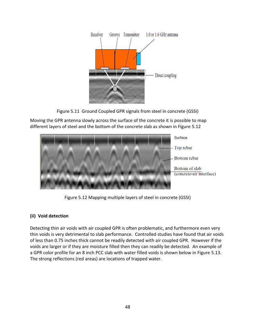
5.3.3 Examples of Analysis of GPR data for PCC pavements The most popular applications of GPR in evaluating concrete pavements when making pavement rehabilitation decisions are a) measuring slab thickness, b) detecting the presence and depth of reinforcing steel and c) identify problems beneath the slab such as voids or trapped moisture. In several instances especially for steel detection the ground coupled systems performed better than the air coupled. The high frequency ground coupled systems such as the 1.5 GHz unit shown in Figure 5.2 can give more focus and better target resolution than air coupled units. Several case studies are shown below. (i) Rebar detection The GSSI handbook on Radar Inspection of GPR has some very good examples on rebar detection. The figure below shows the typical GPR signature obtained over reinforcing steel. There is a hyperbola shape and the top of the hyperbola is the location of the steel. The surface of the concrete is the “direct couple” signature and the depth between the surface and the top of the hyperbola is the depth of concrete cover. GSSI also claim that the size of the rebar can be determined by the shape of the hyperbola.

48

Figure 5.11 Ground Coupled GPR signals from steel in concrete (GSSI)

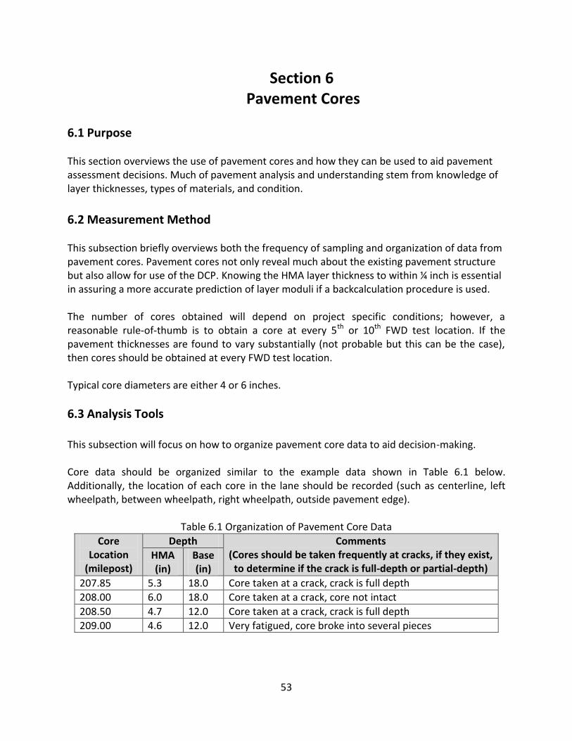
Moving the GPR antenna slowly across the surface of the concrete it is possible to map different layers of steel and the bottom of the concrete slab as shown in Figure 5.12

Figure 5.12 Mapping multiple layers of steel in concrete (GSSI)

(ii) Void detection Detecting thin air voids with air coupled GPR is often problematic, and furthermore even very thin voids is very detrimental to slab performance. Controlled studies have found that air voids of less than 0.75 inches thick cannot be readily detected with air coupled GPR. However if the voids are larger or if they are moisture filled then they can readily be detected. An example of a GPR color profile for an 8 inch PCC slab with water filled voids is shown below in Figure 5.13. The strong reflections (red areas) are locations of trapped water.

49

Figure 5.13 Mapping sub-slab water filled voids with GPR (iii) Deep Investigations of sub slab conditions with GPR The lower frequency ground coupled GPR can be used to investigate deep beneath concrete pavements to identify changes in support conditions and possibly to help explain the occurrence of surface distress. Figure 5.14 shows the color profile from a 400 MHz ground coupled system. The entire pavement system and changes in pavement support can be observed. The transverse rebar can be seen towards the top of the figure. The steel is more closely spaced in the left of the figure. The anomaly on the left is a culvert. The bottom of the slab is indicated. There is a clear change in subgrade support at the top of the subgrade showing the transition from a cut to a fill area.

50

Figure 5.14 Mapping concrete pavements structure with GPR

51

5.4 Implementing GPR technology for Pavement Evaluation

GPR is in excellent technology for inspecting pavements when pavement rehabilitation decisions are being made. Many case studies have been presented over the past two decades but widespread implementation of the technology has been painfully slow. There are several factors causing this and these will be discussed in this section, but the main factors are;

1) The FCC ban on 1 GHz air coupled systems in 2002 (these units can be purchased in any country worldwide except the US). For the past decade most air coupled GPR systems have been performed with systems built before 2002. Only recently have commercial systems become available such as GSSI’s 2.2 GHz as shown in Figure 1. 2) A lack of understanding about what GPR can and cannot do, in many cases the technology was oversold 3) Inadequate data processing software and a lack of end user training

Agencies undertaking GPR implementation should be aware of the following issues which must be resolved before GPR can be implemented as a routine pavement inspection tool; these include

1) Need for GPR hardware specifications 2) Need for data collection software specifications 3) Training/Specifications for data collection activities 4) Specifications/Software for processing and interpreting GPR signals 5) End User training 6) Specifications for output formats and data storage system

Several DOT’s and consultants have implemented GPR technology in-house (for example FDOT and TxDOT and others), but most agencies get GPR services from consultant companies. Selecting the best vendor can also be a problem. (i) Obtaining GPR services The AASHTO publication has a short section with recommendations for agencies on hiring GPR consultants. In initiating contracts the agency has to be convinced that; a) the consultant has quality equipment, ask them to run their equipment against the performance specs (which are available), and b) the consultant has good data processing skills, references from existing customers will help here. GPR interpretation should never be done without taking limited field verification cores early in the project. If the project is for layer thickness determination or for defect detection it should be simple to set up a verification system early in the project.

52

(ii) Barriers to GPR Implementation In addition to the FCC requirements there are also several common misconceptions that must be overcome before any agency will adopt GPR technology; these are a) GPR is only for layer thickness determination: My state has good as-built records so we do not need GPR As stressed throughout this report GPR is much more that a thickness measuring tool. It provides information on the quality of existing structures and helps to explain the causes of pavement distresses. Distresses are often associated with moisture ingress into pavement layers. GPR signals are highly sensitive to moisture in any layer. b) GPR systems are too expensive A complete air coupled system described in this section costs around $100,000 for the complete turnkey system, including vehicle. Ground coupled systems cost approximately $60,000. With the cost of pavement rehabilitation activities these cost are minimal with the cost of rehabilitating sections of Interstate pavement. GPR are substantially less than other nondestructive testing equipment such as FWD’s c) GPR is a black box which is impossible to understand Not true. The basics of GPR are very simple. The key here is that agency personnel should attend training schools to get to understand this technology. Even if the plan is to initiate GPR work through consultants the agency personnel need to have a basic understanding of what this technology can and cannot do. d) Our first experience with GPR was disappointing This is often true. In the early 1990’s a host of companies sold GPR services. They sometimes made extensive claims on GPR’s potential and their ability to successfully interpret the signals. Many claimed to be able to find thin voids beneath concrete pavements often to disappoint the DOT when validation field cores were taken. In some cases the vendors did not have adequate software or interpretation skills. The key here again is training for end user agency personnel. The AASHTO publication also is a good source to identify applications that have a high probability of success e) When the agency initiates a GPR program a host of vendors make claims about their capabilities and it is impossible for the agency to judge their merits. This is often true. But it can be overcome by firstly training of end user agency personnel. Also as with any new technology field verification of any predictions must be a critical part of any program. GPR will not eliminate coring but it will greatly reduce the number of cores

5.5 References GSSI Handbook for Radar Inspection of Concrete, Aug 2006, www.geophysical.com

53

Section 6 Pavement Cores

6.1 Purpose This section overviews the use of pavement cores and how they can be used to aid pavement assessment decisions. Much of pavement analysis and understanding stem from knowledge of layer thicknesses, types of materials, and condition.

6.2 Measurement Method This subsection briefly overviews both the frequency of sampling and organization of data from pavement cores. Pavement cores not only reveal much about the existing pavement structure but also allow for use of the DCP. Knowing the HMA layer thickness to within ¼ inch is essential in assuring a more accurate prediction of layer moduli if a backcalculation procedure is used.

The number of cores obtained will depend on project specific conditions; however, a reasonable rule-of-thumb is to obtain a core at every 5th or 10th FWD test location. If the pavement thicknesses are found to vary substantially (not probable but this can be the case), then cores should be obtained at every FWD test location. Typical core diameters are either 4 or 6 inches.

6.3 Analysis Tools This subsection will focus on how to organize pavement core data to aid decision-making. Core data should be organized similar to the example data shown in Table 6.1 below. Additionally, the location of each core in the lane should be recorded (such as centerline, left wheelpath, between wheelpath, right wheelpath, outside pavement edge).

Table 6.1 Organization of Pavement Core Data

Core Location

(milepost)

Depth Comments (Cores should be taken frequently at cracks, if they exist,

to determine if the crack is full-depth or partial-depth) HMA (in)

Base (in)

207.85 5.3 18.0 Core taken at a crack, crack is full depth

208.00 6.0 18.0 Core taken at a crack, core not intact

208.50 4.7 12.0 Core taken at a crack, crack is full depth

209.00 4.6 12.0 Very fatigued, core broke into several pieces

54

Section 7 Dynamic Cone Penetrometer

7.1 Purpose This section overviews the Dynamic Cone Penetrometer (DCP) and how it can be used to aid pavement assessment decisions.

7.2 Measurement Method

This subsection describes the dynamic cone penetrometer device. The standard test method is:

(iii) ASTM D6951-03: Standard Test Method for Use of the Dynamic Cone Penetrometer in Shallow Pavement Applications

From ASTM D6951: “This test method is used to assess in situ strength of undisturbed soil and/or compacted materials. The penetration rate of the 8-kg DCP can be used to estimate in-situ CBR (California Bearing Ratio), to identify strata thickness, shear strength of strata, and other material characteristics. The 8-kg DCP is held vertically and therefore is typically used in horizontal construction applications, such as pavements and floor slabs. This instrument is typically used to assess material properties down to a depth of 1000-mm (39-in.) below the surface. The penetration depth can be increased using drive rod extensions. However, if drive rod extensions are used, care should be taken when using correlations to estimate other parameters since these correlations are only appropriate for specific DCP configurations. The mass and inertia of the device will change and skin friction along drive rod extensions will occur.”

“The 8-kg DCP can be used to estimate the strength characteristics of fine- and coarse-grained soils, granular construction materials and weak stabilized or modified materials. The 8-kg DCP cannot be used in highly stabilized or cemented materials or for granular materials containing a large percentage of aggregates greater than 50-mm (2-in.). The 8-kg DCP can be used to estimate the strength of in situ materials underlying a bound or highly stabilized layer by first drilling or coring an access hole.”

A sketch of a standard DCP is shown in Figure 7.1.

55

Figure 7.1 Sketch of the Minnesota DOT DCP (from Minnesota DOT, 1993)

56

7.3 Analysis Tools

DCP test results are typically expressed in terms of DPI which is the vertical movement of the DCP cone produced by one drop of the hammer. This is expressed as either mm/hammer blow or inches/hammer blow (Minnesota DOT, 1993).

(i) Basic correlation

A common correlation with DCP data is to estimate the California Bearing Ratio (CBR) of unstabilized materials in a pavement structure. A correlation developed by the U.S. Army Corps of Engineers (Webster et al, 1992) is:

log CBR = 2.46 – 1.12 log(DPI) or CBR = 292/DPI1.12

where DPI = mm/blow

Table 7.1 shows typical CBR and DPI ranges for three soil types (Minnesota DOT, 1993):

Table 7.1 Soils Types, CBR Values, and DPI

Soil Type CBR Range (%)

DPI Range (mm/blow)

Clay (CL) 1-14 15-127

Sand (S-W) 14-39 6-15

Gravel (G-W) 47-95 2.7-5

[The table was modified by the authors of this document so that the DPI and CRB correlation matched.]

(ii) Typical results

Burnham (1997) described an extensive set of DCP measurements on the subgrade soils and base materials used in the various test sections at the Mn/Road facility. These are summarized in Table 7.2. Following this work, the following DPI limits were recommended for use by MnDOT personnel when analyzing DCP results for rehab studies.

Silty/clay materials: DPI 25 mm/blow

Select granular materials: DPI 7 mm/blow

Class 3 Special gradation materials: DPI 5 mm/blow

57

Table 7.2 Minnesota DCP Results Following Placement of the Base Course

Material DPI Avg (mm/blow) (Std Dev)

0-12 inches depth

DPI Avg (mm/blow) (Std Dev)

12-24 inches depth

DPI Avg (mm/blow) (Std Dev)

24-36 inches depth

Clay/Silt Location 1

11 (3)

21 (7)

21 (7)

Clay/Silt Location 2

14 (6)

18 (5)

16 (5)

Clay/Silt Location 3

12 (5)

20 (7)

15 (7)

Sand 5 (2)

5 (1)

6 (2)

Base Course

4 (2)

3 (1)

3

( 1)

[DPI average values were rounded to the nearest whole number.] (iii) Subgrade stability

The Illinois DOT (1982, 2005) has used the DCP to check the subgrade stability. The purpose of this is straightforward—they want to know if the subgrade is stable enough to avoid excessive rutting and/or shoving during and following construction activities. The subgrade IBV (Immediate Bearing Value) can be estimated from the DPI. The IBV is similar to the CBR “except than IBV testing is conducted on a 4-inch molded sample instead of the CBR’s 6-inch sample…further, the penetration test for determining the IBV is conducted immediately after compaction instead of waiting 96 hours—thus IBV and CBR are similar but not identical (Illinois DOT, 2005). Figure 7.2 shows the relationship between unsoaked CBR (actually IBV), DPI, and required thickness of remedial measures. Remedial measures can include the addition of granular backfill or subgrade modification such as lime stabilization. The Illinois DOT DCP results and those from the Minnesota DOT broadly agree in that subgrade DPI values greater than 25 mm/blow are of concern.

58

Figure 7.2 DCP Based Thickness Design for Granular Backfill and Subgrade Modification for

the Illinois DOT (figure from Burnham, 1997 but checked against Illinois DOT, 2005)

(iv) Use of DCP data in renewable decisions

The Texas Transportation Institute developed guidelines for the Texas DOT as to conditions suitable for rubblizing existing rigid pavements (Figure 7.3). The “High Risk” portion of the figure implies the pavement is not a good candidate for rubblization since the supporting base and subgrade is excessively weak. Figure 7.3 is similar to but modified from similar guidelines developed for Illinois (Figure 7.4). Figure 7.4 is of interest since data obtained by Sebesta and Scullion (2007) for US 83 in Texas are plotted by total pavement thickness versus DCP derived CBR values. The DCP—CBR correlation used in Texas is the same as the one described in 6.3(i) which was originally done by the US Army COE.

59

Figure 7.3 Rubblization Selection Chart Developed by TTI (from Sebesta and Scullion, 2007)

60

Figure 7.4 Illinois Rubblization Selection Chart with Data from US 83 (Texas) (from Sebesta and Scullion, 2007; original Illinois DOT criteria from Heckel, 2002)

61

7.4 References

Burnham, T. (1997), “Application of Dynamic Cone Penetrometer to Minnesota Department of Transportation Pavement Assessment Procedures,” Report No. MN/RC 97/19, Minnesota Department of Transportation, St. Paul, MN, May 1997.

Heckel, L (2002), Rubblizing with Bituminous Concrete Overlay—10 Years Experience in Illinois, Report IL-PRR-137, Illinois Department of Transportation, April 2002. [The report contains an appendix entitled Guidelines for Rubblizing PCC Pavement and Designing a Bituminous Overlay. This appendix contains a similar version of Figure 6.4.]

Illinois DOT (1982), “Subgrade Stability Manual,” Policy Mat-10, Illinois Department of Transportation.

Illinois DOT (2005), “Dynamic Cone Penetrometer,” Pavement Technology Advisory PTA-T4, Bureau of Materials and Physical Research, Illinois Department of Transportation, February 2005.

Minnesota DOT (1993), “User Guide to the Dynamic Cone Penetrometer,” Office of Minnesota Road Research, Minnesota DOT.

Sebesta, S. and Scullion, T. (2007), “Field Evaluations and Guidelines for Rubblization in Texas,” Report No. FHWA/TX-08/0-4687-2, Texas Transportation Institute, December 2007.

Webster, S., Grau, R., and Thomas, W. (1992), “Description and Application of Dual Mass Dynamic Cone Penetrometer,” Instruction Report GL-92-3, Waterways Experiment Station, US Army Corps of Engineers, May 1992.

62

Section 8 Subgrade Soil Sampling and Tests

8.1 Purpose This section is used to overview selected elements associated with subgrade soils and what information is needed for pavement assessment decisions. Much of pavement analysis and understanding stem from knowledge of layer thicknesses, types of materials, and condition.

8.2 Measurement Methods This subsection will show both the types of tests and frequency of sampling associated with subgrade soils. A summary of these tests is contained in Table 8.1.

Table 8.1 Summary of Typical Subgrade Tests

Subgrade Test Standard Test Method Purpose of Test

Soil Classification

ASTM D2487-00 Standard Classification of Soils for Engineering Purposes (Unified Soil Classification System)

Soil classification is basic information which can be used to estimate various design-related parameters. The required tests for classification can be used for other determinations (gradation, Atterberg Limits)

California Bearing Ratio

ASTM D1883-07e2 Standard Test Method for CBR of Laboratory-Compacted Soils

Straightforward test for determining relative shear strength of the subgrade soils. CBR can be estimated from a laboratory test or through correlations with devices such as the DCP (Section 7). Caution is needed since laboratory and field produced CBRs can have quite different moisture conditions—hence results.

Resilient Modulus--Laboratory

AASHTO T307 Standard Method of Test for Determining the Resilient Modulus of Soils and Aggregate Materials

If subgrade soil samples are available, laboratory resilient modulus determinations can be made. Triaxial testing is expensive and the results a function of careful sample preparation.

Resilient Modulus—NDT

ASTM D4694-96 Standard Test Method for Deflections with a Falling-Weight-Type Impulse Load Device

The preferred test apparatus for nondestructive testing of pavement structures is the FWD (see Section 4). Straightforward methods for estimating MR are available (Section 4) or backcalculation procedures allow up to 3 pavement layers to be estimated.

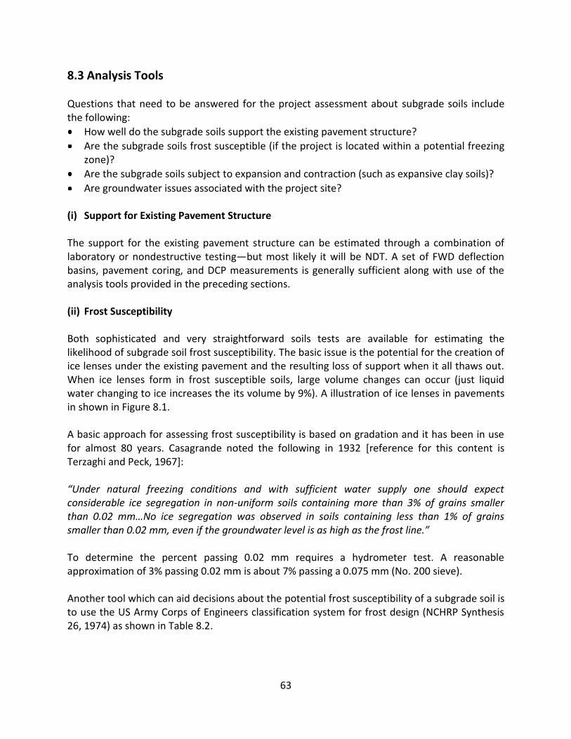
63

8.3 Analysis Tools Questions that need to be answered for the project assessment about subgrade soils include the following:

How well do the subgrade soils support the existing pavement structure?

Are the subgrade soils frost susceptible (if the project is located within a potential freezing zone)?

Are the subgrade soils subject to expansion and contraction (such as expansive clay soils)?

Are groundwater issues associated with the project site? (i) Support for Existing Pavement Structure The support for the existing pavement structure can be estimated through a combination of laboratory or nondestructive testing—but most likely it will be NDT. A set of FWD deflection basins, pavement coring, and DCP measurements is generally sufficient along with use of the analysis tools provided in the preceding sections. (ii) Frost Susceptibility Both sophisticated and very straightforward soils tests are available for estimating the likelihood of subgrade soil frost susceptibility. The basic issue is the potential for the creation of ice lenses under the existing pavement and the resulting loss of support when it all thaws out. When ice lenses form in frost susceptible soils, large volume changes can occur (just liquid water changing to ice increases the its volume by 9%). A illustration of ice lenses in pavements in shown in Figure 8.1. A basic approach for assessing frost susceptibility is based on gradation and it has been in use for almost 80 years. Casagrande noted the following in 1932 [reference for this content is Terzaghi and Peck, 1967]: “Under natural freezing conditions and with sufficient water supply one should expect considerable ice segregation in non-uniform soils containing more than 3% of grains smaller than 0.02 mm…No ice segregation was observed in soils containing less than 1% of grains smaller than 0.02 mm, even if the groundwater level is as high as the frost line.” To determine the percent passing 0.02 mm requires a hydrometer test. A reasonable approximation of 3% passing 0.02 mm is about 7% passing a 0.075 mm (No. 200 sieve). Another tool which can aid decisions about the potential frost susceptibility of a subgrade soil is to use the US Army Corps of Engineers classification system for frost design (NCHRP Synthesis 26, 1974) as shown in Table 8.2.

64

Figure 8.1 Formation of Ice Lenses in a Pavement Structure

65

Table 8.2 US Army Corps of Engineers Frost Design Soil Classification (after US Army, 1990)

Frost Group Soil Type

Percentage finer than 0.02 mm

by weight

Typical soil types under Unified Soil Classification System

Nonfrost Susceptible

(NFS)

(a) Gravels including crushed stone and crushed rock

0 to 1.5 GW, GP

Potentially Frost Susceptible Soils

PFS (a) Gravels

Crushed stone

Crushed rock

1.5 to 3 GW, GP

(b) Sands 3 to 10 SW, SP

S1 Gravelly soils 3 to 6 GW, GP, GW-GM, GP-GM

S2 Sandy soils 3 to 6 SW, SP, SW-SM, SP-SM

F1 Gravelly soils 6 to 10 GM, GW-GM, GP-GM

F1 Gravelly soils 3 to 10 GW, GP, GW-GM, GP-GM

F2 (a) Gravelly soils 10 to 20 GM, GW-GM, GP-GM

(b) Sands 6 to 15 SM, SW-SM, SP-SM

F3 (a) Gravelly soils >20 GM, GC

(b) Sands, except very fine silty sands

>15 SM, SC

(c) Clays, Pl > 12 – CL, CH

F4 (a) All silts – ML, MH

(b) Very fine silty sands >15 SM

(c) Clays, Pl < 12 – CL, CL-ML

(d) Varved clays and other fine-grained, banded sediments

– CL, ML, and SM; CL, CH, and ML; CL, CH, ML, and SM

66

(iii) Expansion and Contraction If these types of soils are present, attempt to answer the following:

Were the subgrade soils previously treated with materials such as lime?

Is the profile of the existing pavement stable? (iv) Groundwater Issues Groundwater issues if apparent, may require the geotechnical engineer to sort out.

8.4 References Terzaghi, K. and Peck, R. (1967), “Soil Mechanics in Engineering Practice,” John Wiley and Sons, 1967. US Army (1990), “ Design of Aggregate Surfaced Roads and Airfields,” Technical Manual TM 5-822-12, Department of the Army, September 1990.

67

Section 9 Traffic Loads for Design

9.1 Purpose This section overviews the use of basic traffic information to estimate design loadings for pavement design. The fundamental parameter that will be estimated is Equivalent Single Axle Loads (ESALs).

9.2 Measurement Method This subsection overviews the kind of traffic information needed to quickly estimate future ESALs. (i) Tire Loads and Terminology Typical truck and bus axles are shown in Figure 9.1 which illustrates single and tandem axles with either single or dual tires. States generally have regulations limiting allowable load per inch width of tire. This tire load limitation varies from a high of 800 lbs/inch to a low of 450 lbs/inch. The primary impact of such state laws has to do with the use of dual or single tires on a specific axle and steer axles.

Single Axle with Dual Tires Single Axle with Single Tires

Tandem Axles with Dual Tires Tandem Axles with Single Tires

Figure 9.1 Illustration of Typical Axle and Tire Configurations

68

(ii) Typical Federal and State Axle Load Limits Typical federal and state axle load limits are:

Single axles: 20,000 lbs

Tandem axles: 34,000 lbs

Total truck gross weight: 80,000 lbs

(iii) FHWA Bridge Formula

A major additional limitation on US trucks and buses is the FHWA Bridge Formula. The total gross weight in pounds imposed on the pavement by any group of two or more consecutive axles on a vehicle or combination of vehicles shall not exceed that weight calculated by use of Equation 9.1 below. The bridge formula is needed since an individual set of bridge design computations cannot be done for every type of truck that may use highways.

Bridge designers use a standard design vehicle for estimating critical stresses, strains, or deflections in a bridge structure. This vehicle is designated HS-20-44 and has been referred to as an umbrella loading. Federal law requires its use in bridge design for the Interstate system.

In effect, the bridge formula helps to ensure bridges are not "overstressed" due to almost infinite number of truck-axle configurations and weights.

W = 500(NL/(N-1) + 12N + 36) Eq. 9.1 Where W = maximum weight on any group of two or more consecutive axles to the nearest 500 lb, L = distance between the extremes of any group of two or more consecutive axles, ft, and N = number of axles in the group under consideration. To illustrate, an example is a 5 axle truck with a 51 ft. separation from the steer axle to the rear

portion of the back tandem. If you wish to know the total vehicle allowable gross weight via the Bridge Formula, then W = 500(5(51)/(5-1) + 12(5) + 36) = 80,000 lb.

(iv) Repetitions of Wheel Loads and ESALs We must be able to convert wheel loads of various magnitudes and repetitions ("mixed traffic") to an equivalent number of "standard" or "equivalent" loads for design purposes. The most commonly used equivalent load is 18,000 lb (80 kN) equivalent single axle loads (normally designated ESAL). The ESAL standard axle load is used in the AASHTO "Guide for Design of Pavement Structures." Wheel load equivalency has been one of the most widely adopted results of the AASHO Road Test (1958 to 1960), i.e., to relate relative damage attributed to axles of different type (single and tandem) and weight. Highway design in most states is based on the ESAL traffic input anticipated over a future 10 to 50 year period.

69

The relationship between repetitions is not arithmetically proportional to the axle loading. Instead, a 10,000 lb single axle needs to be applied to a pavement structure many more than 1.8 times the number of repetitions of an 18,000 lb single axle to have the same effect — in fact, more than 12 times. Similarly, a 22,000 lb single axle needs to be repeated less than half the number of times of an 18,000 lb single axle to have an equivalent effect. A sample of ESAL load equivalency factors is shown in Table 9.1.

Table 9.1 Sample of AASHTO Equivalency Factors

Axle Type (lbs)

Axle Load (lbs)

ESAL Load Equivalency Factors [from AASHTO,

1993] Single axle 2,000

10,000 14,000 18,000 20,000 30,000

0.0003 0.118 0.399 1.000

1.4 7.9

Tandem axle 2,000 10,000 14,000 18,000 20,000 30,000 34,000 40,000 50,000

0.0001 0.011 0.042 0.109 0.162 0.703 1.11 2.06 5.03

A basic element in estimating the future ESALs for a specific project is to forecast the truck and bus volumes for the design (and analysis) period. Once this is done, LEFs in various forms can be applied to the forecast volumes and summed. A complete forecast will include the 13 FHWA vehicle classes (which are not the same vehicle classes as used by vehicle manufacturers). These classes are shown in Table 9.2.

70

Table 9.2 FHWA Vehicle Classes

FHWA Vehicle

Class

Vehicle Class Description

Class 1 Motorcycles (Optional) — All two- or three-wheeled motorized vehicles. Typical vehicles in this category have saddle type seats and are steered by handle bars rather than wheels. This category includes motorcycles, motor scooters, mopeds, motor-powered bicycles, and three-wheel motorcycles. This vehicle type may be reported at the option of the State.

Class 2 Passenger Cars — All sedans, coupes, and station wagons manufactured primarily for the purpose of carrying passengers and including those passenger cars pulling recreational or other light trailers.

Class 3 Other Two-Axle, Four-Tire Single Unit Vehicles — All two-axle, four tire, vehicles, other than passenger cars. Included in this classification are pickups, panels, vans, and other vehicles such as campers, motor homes, ambulances, hearses, and carryalls. Other two-axle, four-tire single unit vehicles pulling recreational or other light trailers are included in this classification.

Class 4 Buses — All vehicles manufactured as traditional passenger-carrying buses with two axles and six tires or three or more axles. This category includes only traditional buses (including school buses) functioning as passenger-carrying vehicles. All two-axle, four-tire single unit vehicles. Modified buses should be considered to be a truck and be appropriately classified.

Class 5 Two-Axle, Six-Tire, Single Unit Trucks — All vehicles on a single frame including trucks, camping and recreational vehicles, motor homes, etc., having two axles and dual rear wheels.

Class 6 Three-Axle Single Unit Trucks — All vehicles on a single frame including trucks, camping and recreational vehicles, motor homes, etc., having three axles.

Class 7 Four or More Axle Single Unit Trucks — All trucks on a single frame with four or more axles.

Class 8 Four or Less Axle Single Trailer Trucks — All vehicles with four or less axles consisting of two units, one of which is a tractor or straight truck power unit.

Class 9 Five-Axle Single Trailer Trucks — All five-axle vehicles consisting of two units, one of which is a tractor or straight truck power unit.

Class 10 Six or More Axle Single Trailer Trucks — All vehicles with six or more axles consisting of two units, one of which is a tractor or straight truck power unit.

Class 11 Five or Less Axle Multi-Trailer Trucks — All vehicles with five or less axles consisting of three or more units, one of which is a tractor or straight truck power unit.

Class 12 Six-Axle Multi-Trailer Trucks — All six-axle vehicles consisting of three or more units, one of which is a tractor or straight truck power unit.

Class 13 Seven or More Axle Multi-Trailer Trucks — All vehicles with seven or more axles consisting of three or more units, one of which is a tractor or straight truck power unit.

71

A somewhat simplified scheme for summarizing the 13 vehicle classes in Table 9.2 is to group all truck and bus traffic into three groups or units as shown in the Table 9.3.

Table 9.3 Simplified Truck and Bus Groups

Simplified Vehicle Categories Groupings of FHWA Vehicle Classes

Single Units which includes

(i) Buses (FHWA Class 4) (ii) 2 axle, 6 tire single units (FHWA Class 5) (iii) 3 axle single units (FHWA Class 6) (iv) 4+ axle single units (FHWA Class 7)

Single Trailers which includes (i) 4 axle single trailer (FHWA Class 8) (ii) 5 axle single trailer (FHWA Class 9) (iii) 6+ axle single trailer (FHWA Class 10)

Multi-Trailers which includes (i) 5 axle multi-trailer (FHWA Class 11) (ii) 6 axle multi-trailer (FHWA Class 12) (iii) 7+ axle multi-trailer (FHWA Class 13)

9.3 Analysis Tools This subsection will focus on how to organize ESAL data so that an overall ESAL estimate for the design period can be made. Table 9.4 shows typical ESALs per vehicle according to the groupings in Table 9.3. The ESALs per vehicle were developed by a State DOT and appear to be typical for US truck traffic. They may appear to be low but the values are averages which include empty backhauls

Table 9.4 ESALs per Vehicle for Simplified Vehicle Groups

Simplified Vehicle Categories

FHWA Classes Average ESALs per Vehicle

Single Unit Trucks 4, 5, 6, 7 0.40

Trucks with Single Trailers 8, 9, 10 1.00

Trucks with Multi-Trailers 11, 12, 13 1.75

Buses (1/2 full) 4 1.60

Thus, if you estimated that a specific highway has daily (one-way) 1,000 single unit trucks, 2,000 trucks with single trailers, and 500 trucks with multi-trailers and no buses, then the daily ESALs would be [1,000(0.4) + 2,000(1.00) + 500(1.75)] = 3,275 ESALs per day or about 1,200,000 ESALs per year. The annual value can be scaled up to the design period with a suitable growth rate (typically 2 to 3 percent).

72

The approximate annual ESALs were estimated for various levels of ADT and are shown in Table 9.5. The primary (and major) assumptions were the typical truck (average over FHWA Classes 4 through 13 based on actual weigh data) has an average ESAL = 1.0. Further, the range of truck percentages as a function of ADT is typically 5 to 10%. Given these assumptions, the following can be used as a guide.

Table 9.5 Approximate Annual ESALs as a Function of ADT

Average Daily Traffic Approximate Annual ESALs

10,000 250,000

25,000 750,000

50,000 1,500,000

100,000 2,500,000

The annual ESALs can vary significantly from the values in Table 9.5. Examples include routes with large numbers of buses which generally have higher ESALs per vehicle than an average truck (often by a factor of two to three or more). The percentage of trucks in the total traffic can vary significantly and particularly so in the vicinity of seaports. Further, rural interstate routes typically have higher percentages of trucks than urban located interstates along with differing mixes of trucks. Urban areas will have higher single unit truck percentages than rural locations. 9.4 References AASHTO (1993), “AASHTO Guide for Design of Pavement Structures, 1993,” American Association of State Highway and Transportation Officials, Washington, DC.

73

Section 10 Construction Productivity and Traffic Impacts

10.1 Purpose This section overviews the various methods for determining construction productivity and traffic impacts of pavement and roadway construction. Traffic impacts can often make up the largest societal cost associated with a paving project sometimes being an order of magnitude more than the agency cost to build/rehabilitate the pavement. An early understanding of productivity and potential traffic impacts can assist the project in determining the most advantageous construction timing, project sequencing (staging) and lane closure scenarios. Often, full roadway closures (in contrast to repeated partial closures) over longer periods of time (e.g., full weekends or multiple days instead of nighttime only closures) can prove to be the least costly alternative if user costs are properly accounted for in construction planning.

10.2 Measurement Methods Traffic impacts are typically quantified by user delay with typical metrics being (1) total user delay, (2) total user cost associated with delay, (3) maximum vehicle queue length, and (4) maximum time in vehicle queue. Usually, the goal of minimizing traffic impacts is interpreted to mean minimizing the total user cost attributable to the existence of the project workzone. Other important considerations (e.g., accident/incident minimization, avoidance of certain public event days that generate high traffic, etc.) may cause the ultimate traffic impacts to be somewhat greater than the optimal minimum. Nonetheless, it is useful to estimate, as accurate as practical considerations allow, the minimum traffic impact scenario for pavement construction. Generally, this estimate uses the following six basic actions: 1. Determine construction productivity. This involves estimating the productivity of basic

construction processes involved in the project such as demolition crew speed/efficiency, dump truck number/capacity, paver speed and materials manufacturing plant productivity. It also involves estimating mobilization/demobilization times, concrete cure time, hot mix asphalt cooling time and traffic control setup time. There may be several estimates of each depending upon the construction scenarios being investigated.

2. Measure existing traffic. While an actual time history is best (e.g., from loop detector

information or manual counts) average daily traffic (ADT) can be used and hourly traffic volumes can be developed multiplying ADT by typical hourly distribution factors for the type of roadway being analyzed.

3. Estimate the fraction of traffic that will cancel their trips and the fraction of traffic that will

use detour routes during the construction. At best, these will be rough estimates unless more sophisticated models are used. These estimates are also highly dependent on the publicity given the roadway work. Values can be obtained from:

a. Agency experience with similar closures and similar publicity in the past. b. A general literature review of similar traffic closures.

74

4. Develop construction scheduling (staging) alternatives. This involves determining the number,

duration and sequence of lane closures required to complete the project. As the traffic impact analysis progresses it is often necessary to refine these alternatives. Strong consideration should be given to scheduling alternatives that result in workzone traffic capacity greater than traffic demand during the hours of work. Essentially, this results in little or no user cost attributed to the roadway work. However, such scheduling alternatives may not exist or be feasible from a construction productivity and/or constructability standpoint. Any number of lane closure scenarios can be considered but it is helpful to at least investigate the following four scenarios: a. Partial night closures: closure only during night hours with light traffic where each roadway

direction is still open although with reduced capacity in at least one direction. These closures are often the first considered since they tend to minimize traffic impacts by only closing lanes when traffic is the lightest. However, they may not provide the lowest user costs because mobilization/demobilization can take up a large percentage of total closure time resulting in low overall productivity. In some scenarios, it may not be possible to make any meaningful progress in a short nighttime closure. Even if partial night closures cannot be used for mainline paving, they are often useful for pre-paving work (e.g., PCC panel sawcutting, restriping lanes, milling HMA, etc.).

b. Full night closures: same as above but with at least one roadway direction fully closed. These may involve detouring an entire direction, counterflowing traffic on one side of a highway or using a pilot car to alternate traffic directions in one lane. Full night closures are sometimes required to do such things as set up counterflow traffic on one side of a roadway or accomplish dangerous overhead work such as overpass demolition/placement.

c. Partial day closures: closure only during day hours with where each roadway direction is still open although with reduced capacity in at least one direction. These closures are often the first considered for lightly trafficked roadways where user delay is unexpected even with some lanes closed. If traffic delays are minimal, day closures can improve safety by providing better visibility and encountering fewer impaired drivers than night work and reduce construction costs by avoiding overtime pay. However, they may not provide the lowest user costs because mobilization/demobilization can take up a large percentage of total closure time resulting in low overall productivity. In some scenarios, it may not be possible to make any meaningful progress in a short day closure.

d. Full day closures: same as above but with at least one roadway direction fully closed. These may involve detouring an entire direction, counterflowing traffic on one side of a highway or using a pilot car to alternate traffic directions in one lane. Full day closures are usually only feasible for lightly trafficked roadways or roadways with large capacity detour routes that do not add significantly to commute time.

e. Partial or full weekend continuous closures: closure starting Friday evening after peak hour traffic and ending Monday morning before peak hour traffic. The typical scenario is a 55-hour weekend closure starting at 9 or 10 p.m. Friday night and ending at 4 or 5 a.m. on Monday morning. The long closure time allows for better productivity because mobilization/demobilization takes up a smaller fraction of total closure time and, more importantly, because construction crews generally get better and faster in their work given

75

a longer working window. Weekends are typically preferred because weekend traffic is usually more discretionary (leading to more canceled trips and less total user delay) and sometimes lighter than weekday traffic.

f. Partial or full week-long continuous closures: closures that are maintained continuously over an entire week (168 hours). While it may not be known if any closure windows will extend over a week or more, estimating this alternative will generally allow estimation of longer closure windows with reasonable accuracy. For instance, the productivity for a 3-week closure is roughly, but not exactly (due to mobilization/demobilization times), three times the productivity of a 1-week continuous closure.

5. Model traffic using the tool of choice (see Analysis Tools Section). This modeling will result in

an estimate of total user cost for the roadway project. In general, larger projects on major routes warrant more modeling while smaller projects on minor routes can often be estimated sufficiently using spreadsheets.

6. Apply FHWA Interim Report Life-Cycle Cost Analysis in Pavement Design (Walls and Smith

1998) standards to estimate user delay cost. This report provides reasonable values for user time (Table 10.1). This table is in 1996 dollars and should be adjusted to current dollars using the Consumer Price Index (CPI). A simple calculator is available from the U.S. Bureau of Labor Statistics (BLS) at: http://www.bls.gov/data/inflation_calculator.htm. Multiplying these values by total delay for each class of vehicle gives an estimate of total workzone user delay cost.

Table 10.1 Recommended Values of Time (from Walls and Smith 1998)

Vehicle Class

$ Value per Vehicle Hour (1996 dollars)

Value Range

Passenger Vehicles $11.58 $10 to 13

Single-Unit Trucks $18.54 $17 to 20

Combination Trucks $22.31 $21 to 24

(i) General Guidance The following general guidance for traffic impacts comes largely from the guidance documents listed in the references portion of this section: Closure Scenarios

Productivity is usually much higher and worker safety is greater with longer, more complete closures, e.g., full closures, weekend closures, etc. (FHWA 2003)

The public is generally very accepting of full closures or a few longer duration closures as an alternative to lengthy schedules of night or day closures (FHWA 2003).

As a work zone remains in effect for a longer period of time (e.g., over several days or several weekends) the fraction of drivers either canceling their trips or taking the detour

76

route is likely to decrease as drivers become used to the situation or determine that a trip can no longer be put off.

Detour routes may experience several times their normal traffic volumes (Lee and Harvey 2006; Lee et al. 2001). It may be prudent to improve detour route capacity through additional lanes, a temporarily reversible lane, signal retiming or other improvements (FHWA 2003).

For major highway jobs, the construction of one lane usually requires a second adjacent lane for access. This means either using an existing wide shoulder (e.g., 10 ft shoulder) if one exists or closing a second lane (Lee 2008).

For major highway jobs, if the lane under construction has more than one major activity underway on it simultaneously (e.g., demolition and paving) a second access lane will likely be needed to avoid stationary trucks in the adjacent lane (Lee 2008).

Avoid creating work zones with live traffic on both sides (e.g., in the middle lanes in one direction). These generally do not leave workers a safe exit from the work zone if it is compromised.

It may be better to use a simpler lane closure plan that is more easily understood by the public even if it does not result in minimum modeled user delay.

Contracting

Lane rental or time-based bonus/penalty contracts should have a clear clause describing how to address changed conditions or any situation where the owner wishes to add work that impacts productivity (Lee et al. 2007). Often, contractors plan to spend more money than the contract price in order to finish early and receive the bonus. In this scenario, without bonus payments the contractor will lose money.

Contracts that contain bonus/penalty amounts for speed and quality should balance these amounts so that it does not become advantageous to sacrifice one bonus to get the other (Muench et al. 2007). For instance, of a maximum quality bonus/penalty is $3,000 but the maximum speed bonus/penalty is $100,000 then in some scenarios it may be logical to sacrifice a small quality bonus for a large speed bonus.

Productivity

The slowest process in a reconstruction project is often demolition (Lee et al. 2007). If several processes are being done simultaneously, demolition will most often control the overall productivity.

The rate at which dump trucks can be filled by an excavator or milling machine is relatively consistent from job-to-job (Lee et al. 2007). Therefore, the best estimate is often what happened on the previous job. If no local information is available, Lee et al. (2007) provides good baseline estimates.

Production rate is often controlled by access to the construction site and allowances made for traffic (e.g., temporary off-ramps in work zones, separation between work zone and traffic).

77

Workzone Capacity

Work zone capacity is highly variable and only moderately predictable. Work zone capacity can be affected by the number of lanes open, intensity of work, the presence of ramps, fraction of heavy vehicles, lane width, lateral clearance, work zone grade and more. Highway Capacity Manual (HCM) procedures are very rough but the Highway Capacity Manual (HCM) (TRB 2000) does suggest 1,600 passenger cars per lane per hour (pc/ln/hr) be used as a baseline for short-term work zones. Typically this number is adjusted downward based on other factors and can be as low as about half the original value.

The more a work zone can be physically and visually separated from traffic (e.g., semi-permanent barriers like jersey barriers or k-rails instead of traffic cones or barrels) the greater the work zone traffic capacity.

Incidents (i.e., accidents, stalled vehicles, etc.) are one of the largest contributors to work zone user delay because there are fewer lanes (if any) that traffic can use to bypass the incident. Dedicating resources (e.g., incident response vehicle, video cameras, variable message boards, traffic management center) to reduce incidents and clear them more quickly can be a cost effective way to minimize user delay (FHWA 2004).

Publicity

Roadway work and closure publicity can be effective in drastically reducing traffic during work zone closures. Often, several-mile long queues predicted using normal traffic volumes never materialize because many drivers cancel their trips or alter their routes.

Even if a local public information campaign is effective it may still be difficult to get closure information to travelers or freight carriers out of the local area who plan on using the affected roadway.

10.3 Analysis Tools This subsection overviews some of the more popular methods for determining traffic impacts for pavement construction projects and factors that influence the choice of tools. Some key considerations when selecting tools:

How much detail is needed? Work zone characteristics, desired outputs and the stage of planning/design/construction will influence tool choice. Often a simpler tool, with less detail is adequate.

Is the tool calibrated to the local area? If not, results may still be useful, however accuracy may be less than expected or needed.

Is the tool stochastic or deterministic? Construction productivity and traffic can be highly variable and difficult to predict. While a deterministic model can provide a single number it is better to provide a reasonable range of answers in order to capture the variable nature of productivity and traffic.

How much detail does the tool produce? Some tools can only estimate traffic impacts over one 24-hour period while some can estimate over much longer time periods. Some tools can only estimate delay on an hourly basis while some can estimate them in much smaller time

78

increments. Some tools make estimates using one single day’s traffic input while others are able to account for daily, weekly and monthly traffic variations.

(i) Analysis Tools: Construction Productivity

Construction productivity tools discussed are: manual methods, standard estimating software and Construction Analysis for Pavement Rehabilitation Strategies (CA4PRS). Manual method. Demolition and paving productivity estimates can be made manually by comparing productivities of the constituent processes and identifying the limiting factor. There are a few references to help in paving productivity calculations. The National Asphalt Pavement Association (NAPA) publishes Balancing Production Rates in Hot Mix Asphalt Operations (IS 120), which contains a step-by-step guide for determining HMA paving productivity. Several companies also offer custom printed asphalt productivity slide rules that paving companies can purchase and brand to be given out to potential customers. Estimating software. Most estimating software (e.g., Bid2Win, HeavyBid) assists users in calculating the productivity of construction processes. CA4PRS. A Microsoft Access-based software tool that can be used to analyze highway pavement rehabilitation strategies including productivity, project scheduling, traffic impacts, and initial project costs based on input data and constraints supplied by the user. The goal is to help determine roadway rehabilitation strategies that maximize production and minimize costs without creating unacceptable traffic delays. As of 2009, all state transportation departments have free group licenses for CA4PRS. (ii) First Order Productivity Estimates In the early planning stages of a project it may be useful to quickly determine rough construction productivity based on a few known parameters. This section displays productivity graphs produced using CA4PRS with most inputs being held constant a typical values. The purpose of these graphs is only to give a rough estimate of typical productivity. CA4PRS should be used to produce more accurate numbers based on actual site-specific parameters for use in any project planning. In general, most inputs were fixed except for the trucking rates (i.e., removal of demolition from the site and delivery of paving material to the site). Thus, the 95% confidence intervals seen are mostly dependent on these delivery rates. In all cases, a 10-mile stretch of two lanes was analyzed (20 lane-miles total). As with all that data input values, this length of highway and total lane-miles has some influence on productivity. Tables 10.2 through 10.7 show input parameters use in CA4PRS to generate Figures 10.1 through 10.9. Estimates are given for:

Remove-and-replace with PCC. Remove the existing pavement and replace with the same depth of new PCC pavement. Productivity is estimated for sequential operations (only one major operations – demolition or paving – is occurring on the jobsite at any one time) and concurrent operations (both major operations – demolition and paving – are occurring on the jobsite at once, with the appropriate space in between). One lane is paved at a time. Sequential operations require one additional lane shut down for construction access, while concurrent

79

operations require two additional lanes shut down for construction access. Calculations were made for both screed paving (slower) and slipform paving (faster). o Screed paving. Using fixed forms and a screed, this paving is usually slower. Assumes 7.5 yd3

agitating mixers arriving at 10 trucks/hr and only one demolition crew. o Slipform paving. Using a slipform paver, this paving is usually faster. Assumes 8.5 yd3 end

dump trucks arriving at 17 trucks/hr and two demolition crews.

Remove-and-replace with HMA. Remove the existing pavement and replace with the same depth of new HMA pavement. The roadway lanes being paved are fully shut down, only one paver with a 12-ft wide screed is used and HMA is paved in lifts. Lifts are generally 3 inches thick with the exception of the top two lifts, which are either 2 or 1.5 inches thick. A lift is paved for each lane across before the next lift is paved on any lane.

Mill-and-fill with HMA. Remove a predetermined thickness from the existing pavement with a HMA milling machine then replace the same thickness with new HMA. The roadway lanes being paved are fully shut down, only one paver with a 12-ft wide screed is used and HMA is paved in lifts. Lifts are generally 3 inches thick with the exception of the top two lifts, which are either 2 or 1.5 inches thick. A lift is paved for each lane across before the next lift is paved on any lane.

Crack, seat and overlay. Crack and seat the existing PCC pavement then overlay with HMA. The roadway being paved is fully shut down, only one paver with a 12-ft wide screed is used and HMA is paved in lifts. Lifts are generally 3 inches thick with the exception of the top two lifts, which are either 2 or 1.5 inches thick. A lift is paved for each lane across before the next lift is paved on any lane.

Unbonded PCC overlay. Prepare the surface of the existing PCC pavement then overlay with PCC that is not bonded to the existing pavement. This is essentially like the “remove-and-replace with PCC” without the demolition component.

80

Table 10.2. CA4PRS Input Values for Remove-and-Replace with PCC

Input Value Distribution/Comments

Activity Constraints

Mobilization 1.0 hours None - Deterministic

Demobilization 2.0 hours None - Deterministic

Base Paving none N/A

Demo-to-PCC Paving Lag Times for Sequential Method

1.0 hours Triangular (min = 0.5 hrs, max = 1.5 hrs)

Demo-to-PCC Paving Lag Times for Concurrent Method

2.0 hours Triangular (min = 1.0 hrs, max = 3.0 hrs)

Resource Profile

Demolition Hauling Truck

Rated Capacity 18.0 tons 9 yd3 of a 15 yd3 truck filled w/2.0 tons/yd3 material

Trucks/hr/team 10 trucks Triangular (min = 8 trucks, max = 12 trucks)

Packing Efficiency 1.0 None - Deterministic

Number of Teams 1.0 2.0

1 team for screed paving, 2 teams for slipform None – Deterministic

Team Efficiency 0.90 Triangular (min = 0.85, max = 0.95)

Base Delivery Truck None N/A (no base material)

Batch Plant

Capacity 500 yd3/hr None – Deterministic (set high to ensure plant is not the limiting activity)

Number of Plants 1 None - Deterministic

Concrete Delivery Truck

Capacity 7.5 yd3 N/A

Trucks per Hour 10/hr 13/hr

The first rate is for screed paving and the second is for slipform paving. Triangular (min = 8/hr, max = 12/hr) Triangular (min = 15/hr, max = 19/hr)

Packing Efficiency 1.0 None - Deterministic

Paver

Speed 5 ft/min None - Deterministic

Number of Pavers 1 None - Deterministic

Schedule Analysis

Construction Window see graphs

Section Profile see graphs Note: no base material included in graphs

Change in Roadway Elevation

No Change

Lane Widths 12 ft.

Curing Time 12 hours

Working Method see graphs

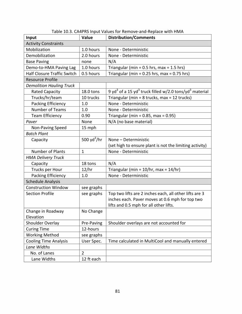
81

Table 10.3. CA4PRS Input Values for Remove-and-Replace with HMA

Input Value Distribution/Comments

Activity Constraints

Mobilization 1.0 hours None - Deterministic

Demobilization 2.0 hours None - Deterministic

Base Paving none N/A

Demo-to-HMA Paving Lag 1.0 hours Triangular (min = 0.5 hrs, max = 1.5 hrs)

Half Closure Traffic Switch 0.5 hours Triangular (min = 0.25 hrs, max = 0.75 hrs)

Resource Profile

Demolition Hauling Truck

Rated Capacity 18.0 tons 9 yd3 of a 15 yd3 truck filled w/2.0 tons/yd3 material

Trucks/hr/team 10 trucks Triangular (min = 8 trucks, max = 12 trucks)

Packing Efficiency 1.0 None - Deterministic

Number of Teams 1.0 None - Deterministic

Team Efficiency 0.90 Triangular (min = 0.85, max = 0.95)

Paver None N/A (no base material)

Non-Paving Speed 15 mph

Batch Plant

Capacity 500 yd3/hr None – Deterministic (set high to ensure plant is not the limiting activity)

Number of Plants 1 None - Deterministic

HMA Delivery Truck

Capacity 18 tons N/A

Trucks per Hour 12/hr Triangular (min = 10/hr, max = 14/hr)

Packing Efficiency 1.0 None - Deterministic

Schedule Analysis

Construction Window see graphs

Section Profile see graphs Top two lifts are 2 inches each, all other lifts are 3 inches each. Paver moves at 0.6 mph for top two lifts and 0.5 mph for all other lifts.

Change in Roadway Elevation

No Change

Shoulder Overlay Pre-Paving Shoulder overlays are not accounted for

Curing Time 12-hours

Working Method see graphs

Cooling Time Analysis User Spec. Time calculated in MultiCool and manually entered

Lane Widths

No. of Lanes 2

Lane Widths 12 ft each

82

Table 10.4. CA4PRS Input Values for Mill-and-Fill with HMA

Input Value Distribution/Comments

Activity Constraints

Mobilization 1.0 hours None - Deterministic

Demobilization 2.0 hours None - Deterministic

Mill-to-HMA Paving Lag 1.0 hours Triangular (min = 0.5 hrs, max = 1.5 hrs)

Half Closure Traffic Switch 0.5 hours Triangular (min = 0.25 hrs, max = 0.75 hrs)

Resource Profile

Milling and Hauling

Number of Teams 1.0 None - Deterministic

Team Efficiency 0.90 Triangular (min = 0.85, max = 0.95)

Milling Machine

Class Large

Material Type AC-Hard

Efficiency Factor 0.90 Triangular (min = 0.85, max = 0.95)

Hauling Truck

Rated Capacity 18.0 tons 9 yd3 of a 15 yd3 truck filled w/2.0 tons/yd3 material

Trucks/hr/team 13 trucks Triangular (min = 11 trucks, max = 15 trucks)

Packing Efficiency 1.0 None - Deterministic

Batch Plant

Capacity 500 yd3/hr None – Deterministic (set high to ensure plant is not the limiting activity)

Number of Plants 1 None - Deterministic

HMA Delivery Truck

Capacity 18 tons N/A

Trucks per Hour 12/hr Triangular (min = 10/hr, max = 14/hr)

Packing Efficiency 1.0 None - Deterministic

Paver None N/A (no base material)

Non-Paving Speed 15 mph

Schedule Analysis

Construction Window see graphs

Section Profile see graphs Lifts are between 1.5 and 3 inches. Paver speeds are 0.5 to 0.6 mph.

Change in Roadway Elevation

No Change

Shoulder Overlay Pre-Paving Shoulder overlays are not accounted for

Curing Time 12-hours

Working Method see graphs

Cooling Time Analysis User Spec. Time calculated in MultiCool and manually entered

Lane Widths

No. of Lanes 2

Lane Widths 12 ft each

83

Table 10.5. CA4PRS Input Values for Crack, Seat and Overlay

Input Value Distribution/Comments

Activity Constraints

Mobilization 3.0 hours None - Deterministic

Demobilization 2.0 hours None - Deterministic

Half Closure Traffic Switch 0.5 hours Triangular (min = 0.25 hrs, max = 0.75 hrs)

Resource Profile

Paver None N/A (no base material)

Non-Paving Speed 15 mph

Batch Plant

Capacity 500 yd3/hr None – Deterministic (set high to ensure plant is not the limiting activity)

Number of Plants 1 None - Deterministic

HMA Delivery Truck

Capacity 18 tons N/A

Trucks per Hour 12/hr Triangular (min = 10/hr, max = 14/hr)

Packing Efficiency 1.0 None - Deterministic

Schedule Analysis

Construction Window see graphs

Section Profile see graphs Top two lifts are 2 inches each, all other lifts are 3 inches each. Paver moves at 0.6 mph for top two lifts and 0.5 mph for all other lifts.

Change in Roadway Elevation

No Change

Shoulder Overlay Pre-Paving Shoulder overlays are not accounted for

Curing Time 12-hours

Working Method see graphs

Cooling Time Analysis User Spec. Time calculated in MultiCool and manually entered

Lane Widths

No. of Lanes 2

Lane Widths 12 ft each

84

Table 10.6. CA4PRS Input Values for Unbonded PCC Overlay

Input Value Distribution/Comments

Activity Constraints

Mobilization 3.0 hours None - Deterministic (longer time accounts for surface preparation)

Demobilization 2.0 hours None - Deterministic

Base Paving none N/A

Demo-to-PCC Paving Lag Times for Sequential Method

0 hours No demolition occurs

Demo-to-PCC Paving Lag Times for Concurrent Method

0 hours No demolition occurs

Resource Profile

Demolition Hauling Truck High numbers are a work-around to make demolition take essentially no time

Rated Capacity 100.0 tons None - Deterministic

Trucks/hr/team 100 trucks None - Deterministic

Packing Efficiency 1.0 None - Deterministic

Number of Teams 100.0 None - Deterministic

Team Efficiency 1.00 None - Deterministic

Base Delivery Truck None N/A (no base material)

Batch Plant

Capacity 500 yd3/hr None – Deterministic (set high to ensure plant is not the limiting activity)

Number of Plants 1 None - Deterministic

Concrete Delivery Truck

Capacity 7.5 yd3 N/A

Trucks per Hour 10/hr Triangular (min = 8/hr, max = 12/hr)

Packing Efficiency 1.0 None - Deterministic

Paver

Speed 5 ft/min None - Deterministic

Number of Pavers 1 None - Deterministic

Schedule Analysis

Construction Window see graphs

Section Profile see graphs Note: no base material included in graphs

Change in Roadway Elevation

No Change

Lane Widths 12 ft.

Curing Time 12 hours

Working Method see graphs

85

Table 10.7. MultiCool Input Parameters for HMA Options

Input Value

Constant Inputs in All Scenarios

Start Time 1000, 7/15/2010

Environmental Conditions

Ambient Air Temp. 60°F

Average Wind Speed 5 mph

Sky Conditions Clear&Dry

Latitude 38° North

Existing Surface

Material Type Granular Base

Moisture Content Dry

State of Moisture Unfrozen

Surface Temp. 60°F

Mix Specifications

Mix Type Dense Graded

PG Grade 64-22

Delivery Temp. 300°F

Stop Temp. 140°F

Lift Thicknesses

3 inches of HMA total 2 lifts of 1.5 inches each

6 inches of HMA total 3 lifts of 2 inches each

9 inches of HMA total 3 lifts of 2 inches, 1 lift of 3 inches

12 inches of HMA total 2 lifts of 1.5 inches 3 lifts of 3 inches

86

Figure 10.1. Productivity estimates for remove-and-replace with PCC (fixed form) using sequential operations. Solid lines indicate averages and dashed lines indicate 95% confidence intervals. Note:

this option is not feasible using 10-hour night closures.

0

2

4

6

8

10

12

14

0.0 0.5 1.0 1.5 2.0 2.5 3.0 3.5 4.0 4.5 5.0

Thic

kne

ss o

f P

ave

me

nt

Co

nst

ruct

ed

(in

che

s)

Lanes-MIles Constructed in One Closure

10-hour Night Closure (not feasible)

55-hour Weekend Closure

168-hour 24/7 Continuous Week-Long Closure

87

Figure 10.2. Productivity estimates for remove-and-replace with PCC (slipform) using sequential operations. Solid lines indicate averages and dashed lines indicate 95% confidence intervals. Note: this option is not feasible using 10-hour night closures.

0

2

4

6

8

10

12

14

0.0 1.0 2.0 3.0 4.0 5.0 6.0 7.0

Thic

kne

ss o

f P

ave

me

nt

Co

nst

ruct

ed

(in

che

s)

Lanes-MIles Constructed in One Closure

10-hour Night Closure (not feasible)

55-hour Weekend Closure

168-hour 24/7 Continuous Week-Long Closure

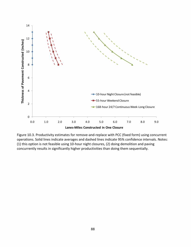
88

Figure 10.3. Productivity estimates for remove-and-replace with PCC (fixed form) using concurrent operations. Solid lines indicate averages and dashed lines indicate 95% confidence intervals. Notes: (1) this option is not feasible using 10-hour night closures, (2) doing demolition and paving concurrently results in significantly higher productivities than doing them sequentially.

0

2

4

6

8

10

12

14

0.0 1.0 2.0 3.0 4.0 5.0 6.0 7.0 8.0 9.0

Thic

kne

ss o

f P

ave

me

nt

Co

nst

ruct

ed

(in

che

s)

Lanes-MIles Constructed in One Closure

10-hour Night Closure (not feasible)

55-hour Weekend Closure

168-hour 24/7 Continuous Week-Long Closure

89

Figure 10.4. Productivity estimates for remove-and-replace with PCC (slipform) using concurrent operations. Solid lines indicate averages and dashed lines indicate 95% confidence intervals. Notes:

(1) this option is not feasible using 10-hour night closures, (2) doing demolition and paving concurrently results in significantly higher productivities than doing them sequentially.

0

2

4

6

8

10

12

14

0.0 2.0 4.0 6.0 8.0 10.0 12.0

Thic

kne

ss o

f P

ave

me

nt

Co

nst

ruct

ed

(in

che

s)

Lanes-MIles Constructed in One Closure

10-hour Night Closure (not feasible)

55-hour Weekend Closure

168-hour 24/7 Continuous Week-Long Closure

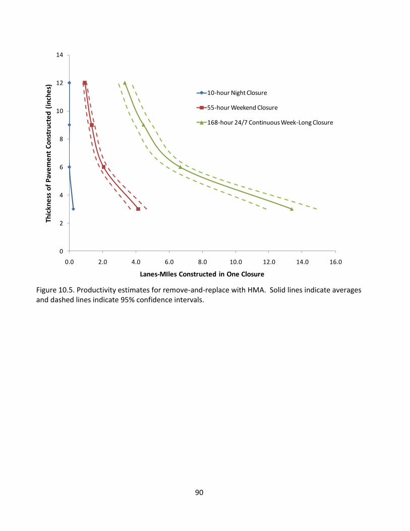
90

Figure 10.5. Productivity estimates for remove-and-replace with HMA. Solid lines indicate averages and dashed lines indicate 95% confidence intervals.

0

2

4

6

8

10

12

14

0.0 2.0 4.0 6.0 8.0 10.0 12.0 14.0 16.0

Thic

kne

ss o

f P

ave

me

nt

Co

nst

ruct

ed

(in

che

s)

Lanes-MIles Constructed in One Closure

10-hour Night Closure

55-hour Weekend Closure

168-hour 24/7 Continuous Week-Long Closure

91

Figure 10.6. Productivity estimates for mill-and-fill with HMA. Solid lines indicate averages and dashed lines indicate 95% confidence intervals.

0

1

2

3

4

5

6

7

0.0 5.0 10.0 15.0 20.0 25.0

Thic

kne

ss o

f P

ave

me

nt

Co

nst

ruct

ed

(in

che

s)

Lanes-MIles Constructed in One Closure

10-hour Night Closure

55-hour Weekend Closure

168-hour 24/7 Continuous Week-Long Closure

92

Figure 10.7. Productivity estimates for crack, seat and overlay. Solid lines indicate averages and dashed lines indicate 95% confidence intervals.

0

1

2

3

4

5

6

7

8

9

10

0.0 5.0 10.0 15.0 20.0 25.0 30.0 35.0 40.0

Thic

kne

ss o

f P

ave

me

nt

Co

nst

ruct

ed

(in

che

s)

Lanes-MIles Constructed in One Closure

10-hour Night Closure

55-hour Weekend Closure

168-hour 24/7 Continuous Week-Long Closure

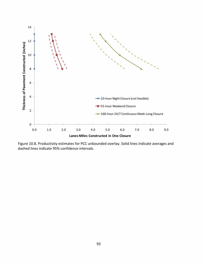
93

Figure 10.8. Productivity estimates for PCC unbounded overlay. Solid lines indicate averages and dashed lines indicate 95% confidence intervals.

0

2

4

6

8

10

12

14

0.0 1.0 2.0 3.0 4.0 5.0 6.0 7.0 8.0 9.0

Thic

kne

ss o

f P

ave

me

nt

Co

nst

ruct

ed

(in

che

s)

Lanes-MIles Constructed in One Closure

10-hour Night Closure (not feasible)

55-hour Weekend Closure

168-hour 24/7 Continuous Week-Long Closure

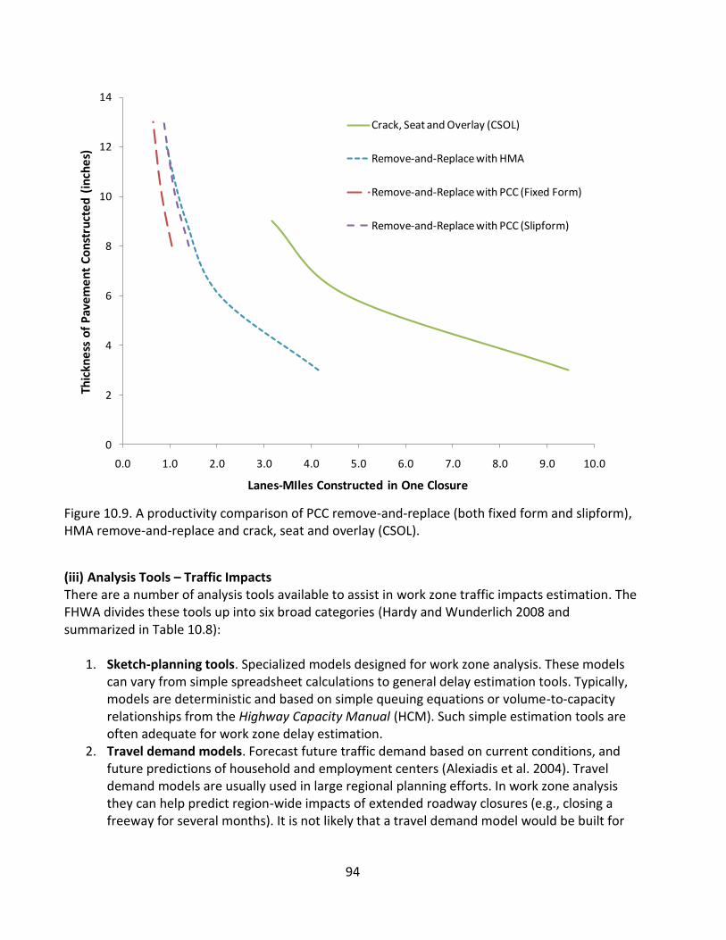
94

Figure 10.9. A productivity comparison of PCC remove-and-replace (both fixed form and slipform), HMA remove-and-replace and crack, seat and overlay (CSOL).

(iii) Analysis Tools – Traffic Impacts There are a number of analysis tools available to assist in work zone traffic impacts estimation. The FHWA divides these tools up into six broad categories (Hardy and Wunderlich 2008 and summarized in Table 10.8):

1. Sketch-planning tools. Specialized models designed for work zone analysis. These models can vary from simple spreadsheet calculations to general delay estimation tools. Typically, models are deterministic and based on simple queuing equations or volume-to-capacity relationships from the Highway Capacity Manual (HCM). Such simple estimation tools are often adequate for work zone delay estimation.

2. Travel demand models. Forecast future traffic demand based on current conditions, and future predictions of household and employment centers (Alexiadis et al. 2004). Travel demand models are usually used in large regional planning efforts. In work zone analysis they can help predict region-wide impacts of extended roadway closures (e.g., closing a freeway for several months). It is not likely that a travel demand model would be built for

0

2

4

6

8

10

12

14

0.0 1.0 2.0 3.0 4.0 5.0 6.0 7.0 8.0 9.0 10.0

Thic

kne

ss o

f P

ave

me

nt

Co

nst

ruct

ed

(in

che

s)

Lanes-MIles Constructed in One Closure

Crack, Seat and Overlay (CSOL)

Remove-and-Replace with HMA

Remove-and-Replace with PCC (Fixed Form)

Remove-and-Replace with PCC (Slipform)

95

the specific purpose of work zone traffic analysis. Rather, an existing model may be used if available and warranted.

3. Traffic signal optimization tools. Used to develop signal timing plans. These can be useful if a temporary signal is used or if signals are retimed to accommodate work zone traffic or increased detour route traffic.

4. Macroscopic simulation models. Based on the deterministic relationships of traffic speed, flow and density (Alexiadis et al. 2004). These models treat flow as an aggregate quantity in a defined area and do not track individual vehicles. They are useful for modeling larger area impacts of work zones because of their aggregate nature.

5. Mesoscopic simulation models. Represent relative flow of vehicles on a network but do not model individual lanes or vehicles. These models are between macroscopic and microscopic models in detail. These models can simulate both large geographic areas as well as specific corridors. They do not, however possess the detail to model more detailed strategies such as signal timing. These models require large amounts of data.

6. Microscopic simulation models. Simulate the movement of individual vehicles. These models require large amounts of data and can get unwieldy when attempting to simulate a large network. Often these models can provide animated output which can clearly communicate to decision-makers and the public what the potential traffic impacts of modeled actions will be.

Table 10.8. Traffic Model Types for Work Zone Traffic Impacts

Model Type Examples Strengths Weaknesses

Sketch-planning HDM, QUEWZ-98, QuickZone, CA4PRS

Low cost, specific to work zones, fast

Limited modeling ability, not well supported

Travel demand EMME/2, TransCAD, TRANSIMS

Can model large areas Low detail, cannot model short term work zone effects

Signal optimization PASSER, Synchro Models signal timing and coordination

Does not model other things

Macroscopic BTS, KRONOS, METACORE/METANET, TRANSYT-7F

Can model large areas Low detail, cannot model short term work zone effects

Mesoscopic CONTRAM, DYNASMART, DYNAMIT, MesoTS

Good compromise between macro- and micro models

Data intensive

Microscopic CORSIM, VISSIM, PARAMICS

Can model small details, good communication tool

Data intensive

96

The most appropriate modeling approach depends upon (Hardy and Wundurlich 2008):

Work zone characteristics. The expected level of impact a work zone will have on travelers including the geographic scale of affected area and complexity of the road network within this area.

Transportation management plan strategies. The means by which traffic will be managed including such items as lane closures, full roadway closures, lane shifts, counterflow traffic, night/day work, detours, weekend work, etc.

Data availability and quality. The type, amount, accuracy and timeliness of available data.

Agency resources. The owner agency’s funding, technical staff, and schedule.

Work zone performance measures. The performance measures selected by the owner agency to quantify traffic impacts. Typically this is some form of delay (in minutes or cost) either in total (total delay/cost) or peak (longest queue, longest wait).

Since the use of modeling tools beyond sketch-planning tools will almost surely require traffic expertise beyond the pavement profession, further discussion is limited to a few sketch-planning tools that may be of use: QuickZone and CA4PRS. Both of these tools can provide meaningful traffic impact estimates for a relatively small money and time investment. QuickZone 2.0. A Microsoft Excel-based tool (requires Excel 97 as a minimum) that estimates work zone traffic impacts. It allows the user to input a node-and-link network (see Figures 10.10 and 10.11) then assign traffic counts to that network. It can coarsely simulate traffic variations between days of the week, and months of the year by applying multiples to standard average daily traffic (ADT) inputs. It can simulate multiple lane closures over time, model traffic over an entire week (Figure 10.12) and display various traffic impact metrics (Figure 10.13). These capabilities are helpful because they allow QuickZone to show difference in traffic impacts between nights and days, weekends and weekdays, and seasons (e.g., summer vs. fall work). The user guide explains the algorithm QuickZone uses to estimate delay and user cost but specific equations are not listed or discussed. QuickZone is inexpensive (about $200) but is getting relatively old (version 2.0 was released in 2005) without any significant upgrade or support beyond a user guide. Simple scenarios with just a few links and nodes are relatively easy to simulate, however more complex scenarios become cumbersome due to tedious data entry and difficult input troubleshooting if outputs are suspect.

97

Figure 10.10 A simple network that works quite well in QuickZone.

Figure 10.11. A complex network simulation in QuickZone (I-5 in the Seattle, WA area is shown). This network simulation exposed several program bugs, was unwieldy to process and required tedious troubleshooting to make operational. This level of complexity is not recommended.

98

Figure 10.12. Unedited QuickZone 2.0 simulation output chart for a one-week time period. Note that the automatic graph labeling on the horizontal axis is unreadable, however this can be corrected by editing the graph in Excel.

Figure 10.13. QuickZone 2.0 summary tables showing available traffic impact metrics. CA4PRS. A Microsoft Access-based software tool that can be used to analyze highway pavement rehabilitation strategies including productivity, project scheduling, traffic impacts, and initial

0.00

2.00

4.00

6.00

8.00

10.00

12.00

14.00

16.00

18.00

20.00

Qu

eu

e L

en

gth

(M

ile

s)

Time of Day

After Case Queue Length (Miles) for Inbound Direction from Phase Monday 8am to Saturday midnight

Reconstruction area (70-73.64)

Period with highest delay in After Case

Phase

2 - Sunday

midnight to

Thursday 8am

Direction Inbound

Day/Time Sunday 21:00

Max Queue (Miles) Max Delay (min) Passenger Cars Truck Detour Econ/Misc Total

Baseline 0 0 $0 $0 $0 $0 $0

After 34.13 778.23 $22,036,199 $1,851,536 $0 $0 $23,887,735

Total 34.13 778.23 $22,036,199 $1,851,536 $0 $0 $23,887,735

Total Project User Cost ($)

99

project costs based on input data and constraints supplied by the user. The traffic impacts analysis portion of CA4PRS (Labeled “Work-Zone Analysis in the software) can simulate 24 hours of traffic through a defined work zone. Work zones are defined by the number of lanes closed, closure duration and work zone capacity (Figure 10.14). Traffic can be entered by hourly count or ADT can be entered and then distributed over 24 hours using hourly factors. CA4PRS can simulate one lane closure scenario over a 24-hour period. Longer closures are estimated by multiplying the results of one 24-hour analysis by the total number of closures. The 24-hour simulation limit using only one traffic count makes it difficult to account for longer closures (e.g., over several weeks or months) where traffic flow is likely to change over time (e.g., weekday vs. weekend or summer vs. fall). Output is similar to that of QuickZone (Figures 10.15 and 10.16). Currently, the CA4PRS user manual does not explain the delay estimation algorithm it uses. As of 2010, CA4PRS development is ongoing and licenses for state DOTs are free. CA4PRS only models traffic in the work zone and does not model any wider network.

Figure 10.14 CA4PRS Work-Zone Analysis input screen.

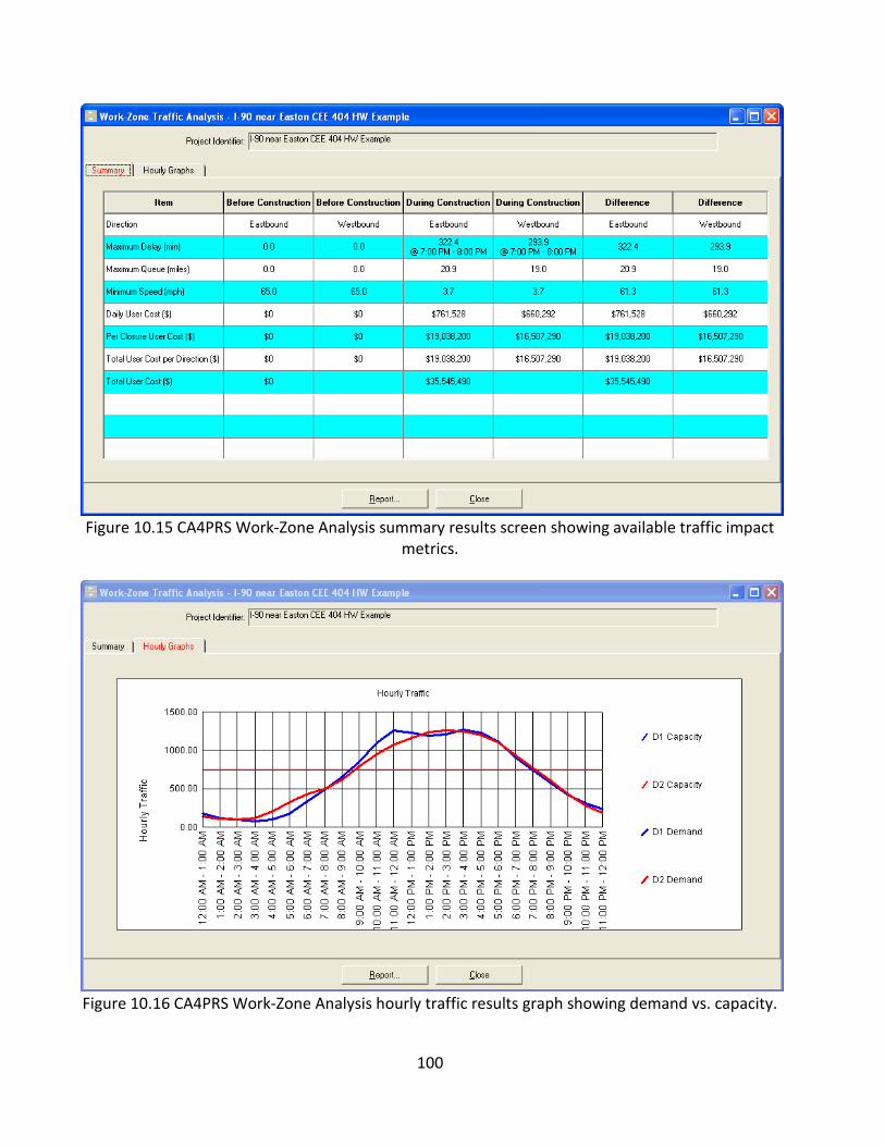
100

Figure 10.15 CA4PRS Work-Zone Analysis summary results screen showing available traffic impact

metrics.

Figure 10.16 CA4PRS Work-Zone Analysis hourly traffic results graph showing demand vs. capacity.

101

10.4 References Alexiadis, V.; Jeannotte, K. and Chandra, A. (2004). Traffic Analysis Toolbox Volume I: Traffic Analysis Tools Primer. FHWA-HRT-04-038. Federal Highway Administration (FHWA), U.S. Department of Transportation, Washington, D.C.

Federal Highway Administration (FHWA). (2003). Full Road Closure for Work Zone Operations: A Cross-Cutting Study. http://ops.fhwa.dot.gov/wz/resources/publications/FullClosure/CrossCutting/its.htm

Hardy, M. and Wunderlich, K. (2008). Traffic Analysis Toolbox Volume VIII: Work Zone Modeling and Simulation – A Guide for Decision Makers. FHWA-HOP-08-029. Federal Highway Administration (FHWA), U.S. Department of Transportation, Washington, D.C.

Hardy, M. and Wunderlich, K. (2008). Traffic Analysis Toolbox Volume IX: Work Zone Modeling and Simulation – A Guide for Analysts. FHWA-HOP-09-001. Federal Highway Administration (FHWA), U.S. Department of Transportation, Washington, D.C.

Lee, E.B. and Ibbs, C.W. (2005). Computer Simulation Model: Construction Analysis for Pavement Rehabilitation Strategies. Journal of Construction Engineering and Management, 131(4), p. 449-458.

Lee, E.B.; Harvey, J.T. and Thomas, D. (2005). Integrated Design/Construction/Operations Analysis for Fast-Track Urban Freeway Reconstruction. Journal of Construction Engineering and Management, 131(12), p. 1283-1291.

Lee, E.B.; Lee H.; and Ibbs, C.W. (2007). Productivity Aspects of Urban Freeway Rehabilitation with Accelerated Construction Journal of Construction Engineering and Management, 133(10), p. 798-806.

Lee, E.B.; Lee, H. and Harvey, J.T. (2006). Fast-Track Urban Freeway Rehabilitation with 55 h Weekend Closures: I-710 Long Beach Case Study. Journal of Construction Engineering and Management, 132(5), p. 465-472.

Lee, E.B.; Roesler, J.R.; Harvey, J.T. and Ibbs, C.W. (2001). Case Study of Urban Concrete Pavement Reconstruction and Traffic Management for the I-10 ( Pomona, CA) Project. University of California, Berkeley Institute of Transportation Studies, Pavement Research Center. Report for the Innovative Pavement Research Foundation (IPRF), Falls Church, VA.

Muench, S.T.; Ozolin, B. Uhlmeyer, J. and Pierce, L.M.(2007). Rapid Concrete Panel Replacement in Washington State: Lessons Learned. International Conference on Optimizing Paving Concrete Mixtures and Accelerated Concrete Pavement Construction and Rehabilitation, 7-9 November 2007, Atlanta, GA

102

Lee, E.B.; Roesler, J.R.; Harvey, J.T. and Ibbs, C.W. (2002). Case Study of Urban Concrete Pavement Reconstruction on I-10. Journal of Construction Engineering and Management, 128(1), p. 49-56.

National Asphalt Pavement Association (NAPA). (1996). Balancing Production Rates in Hot Mix Asphalt Operations , IS-120. NAPA, Landham, MD.

Walls, J. and Smith, M.R. (1998). Life-Cycle Cost Analysis in Pavement Design. Report No. FHWA-SA-98-079. FHWA, Washington, D.C. http://isddc.dot.gov/OLPFiles/FHWA/013017.pdf

Lee, E.B.; Ibbs, C.W. and Thomas, D. (2005). Minimizing Total Cost for Urban Freeway Reconstruction with Integrated Construction/Traffic Analysis. Journal of Infrastructure Systems, 11(4), pp. 250-257.

Maze, T.H.; Schrock, S.D. and Kamyab, A. (2000). Capacity of Freeway Work Zone Lane Closures. Mid-Continent Transportation Symposium 2000 Proceedings. http://www.ctre.iastate.edu/pubs/midcon/Maze.pdf.

Kim, T.; Lovell, D.J. and Paracha, J. (2001). A New Methodology to Estimate Capacity for Freeway Work Zones. Presentation at the 2001 Transportation Research Board Annual Meeting, Washington D.C. http://www.workzonesafety.org/files/documents/database_documents/00675.pdf.

Borchardt, D.W.; Geza, P.; Sun, D. and Ding, L. (2009). Capacity and Road User Cost Analysis of Selected Freeway Work Zones in Texas. FHWA/TX-09/0-5619-1. Texas Department of Transportation, Austin, TX. http://tti.tamu.edu/documents/0-5619-1.pdf.

Lee, E.B. (2008). CA4PRS User Manual (Version 2.1). University of California, Berkeley, Berkeley, CA.

Transportation Research Board (TRB). (2000). Highway Capacity Manual (HCM2000). TRB, National Research Council, Washington, D.C.

Federal Highway Administration (FHWA). (2004). Intelligent Transportation Systems in Work Zones: Keeping Traffic Moving During Reconstruction of the Big I, a Major Interstate-Interstate Interchange in Albuquerque. FHWA, U.S. Department of Transportation, Washington, D.C.

103

Section 11 Life Cycle Assessment (Environmental Accounting)

11.1 Purpose This section overviews a method for determining the inputs and outputs of a pavement system that are relevant to the environment. This can include, but is not limited to: energy use, water use, emissions, raw materials and human health impacts. This method, called life cycle assessment (LCA) is essentially an environmental accounting protocol. LCA results can be used as part of the decision-making process when determining the appropriate pavement rehabilitation/reconstruction strategy. For instance, if an owner-agency must comply with a greenhouse gas (GHG) reduction mandate, options resulting in less GHG may be considered more favorably. Often, but not always, environmental accounting results tend to agree with life-cycle assessment results in pavement construction scenarios. In the future, it is likely that energy and emissions associated with roadway construction, or any industry, will be scrutinized more carefully. Green house gas (GHG) emissions are likely to be subject to a cap-and-trade scheme in the U.S. and are increasingly being addressed through the National Environmental Policy Act (NEPA) as recent White House Council on Environmental Quality (CEQ) guidance shows (Sutley 2010). As this scrutiny increases, there will likely be more tools to help in analysis. It also seems plausible that once industry has a fair idea what energy, emissions and other resources are associated with roadway construction, it will begin to adopt (either voluntarily or by regulation) efficiency standards associated with these items similar to what has happened with the automobile industry (i.e., fuel efficiency standards), power generation (i.e., clean energy portfolio requirements) and even toilets (i.e., maximum allowable flow).

11.2 Measurement Methods (i) Introduction A LCA attempts to identify inputs and outputs of a system that are relevant to the environment from its inception to its ultimate disposition. This means that a LCA includes everything from gathering raw materials to the point at which those materials are returned to the environment. This collection of all processes from “cradle to grave” allows LCA to provide a cumulative total of inputs and outputs (e.g., energy, emissions, water, use, etc.) for a final product and the environmental impacts associated with those inputs and outputs. The resulting environmental impacts of these cumulative inputs and outputs is assessed and results can be used to compare alternatives and improve the system. The International Standards Organization (ISO) outlines a systematic four phased approach:

1. Goal and scope. Define the reasons for carrying out the LCA, the intended audience,

geographic and temporal considerations, system functions and boundaries, impact assessment and interpretation methods.

104

2. Inventory assessment. Quantify life cycle energy use, emissions, and land and water use for technology use in each life cycle stage.

3. Impact assessment. Estimate the impacts of inventory results. 4. Interpretation. Investigate the contribution of each life cycle stage, technology use

throughout the life cycle and include data quality, sensitivity and uncertainty analyses. LCA in general, and for pavements in particular, is still in a relatively early stage of development and thus common practices are still developing and available data can be sparse. This presents problems when using LCA as a decision support tool; especially when comparing alternatives. Results using different data sets, methods and practices can be an order of magnitude different for the same analyzed pavement section. Common issues with LCA include:

Data sources. Often LCA data come from a select few databases such as the U.S. Life-Cycle Inventory Database (from NREL), ecoinvent, ELCD database, etc. These are generally reviewed for accuracy/errors and can help standardize information for use in LCAs. However, data usually come from many different sources beyond these ranging from personal observation to national databases, which can lead to problems when comparing one LCA with another. For instance, the CO2 associated with hot mix asphalt (HMA) production is not a universal constant, but rather it varies depending upon plant type, components and manufacturer, aggregate moisture content, fuel type, amount of reclaimed asphalt (RAP) included, asphalt binder grade, crude oil source, regional electricity mix, etc. While databases of national averages can lead to some consistency in results between LCAs, they often do not provide the detail necessary to distinguish between process changes (e.g., using warm mix asphalt or not), especially at the local project level. At the very least, a LCA should clearly identify its data sources.

Missing data. There are many industrial processes where some, if not all, relevant data are not known, recorded, or made available for public use. For instance, the amount of fugitive dust on site associated with pavement construction is not generally known. Or, the exact chemical make-up of an asphalt modifier may be a trade secret that the manufacturer is not willing to divulge.

Outdated data. Sometimes, data exist but are outdated. Over time, processes change, equipment improves, raw material sources change, etc.

Data specificity. While general average data may be more readily available or lead to more consistency between LCAs, it often does not contain the detail needed to distinguish between two alternatives being considered. For instance, the EPA’s AP-42 document contains average emissions data for asphalt plants; however, it assumes only an average amount of RAP being used at the plant. Therefore, if this data is used it cannot distinguish between a mix using all virgin materials and one using 25 percent RAP, for instance.

Setting boundaries. A LCA that attempts to account for all processes associated with a system can quickly become intractable. For example, one could account for the slipform paver and its energy use and emissions associated with a concrete pavement. One could also account for the energy and emissions associated with manufacturing that slipform paver. However that leads to potentially considering the energy and emissions associated with the manufacture of the machines that made the paver and so on. For another example, one can choose whether to include the effect of pavement stiffness on the rolling resistance it offers to vehicles that travel

105

on it. Reduced rolling resistance over the life of a pavement may lead to substantial energy savings when summed over the millions of vehicles that may use the road. However, one might question whether including this effect alone is a realistic assessment of the pavement’s impact on vehicle operations. Because of these boundary issues (what processes are included and excluded), every LCA has a defined boundary (that should be explicitly stated) that details which processes are included and which are not. Inclusions and exclusions are often not consistent between LCAs and can be controversial.

Procedural practices. Most LCAs generally follow ISO 14040 and ISO 14044. However, these standards are still quite generally written and leave much room for interpretation. No set of more precise LCA procedures exist for pavements. For instance, ISO 14044 says that feedstock energy (energy associated with burning the material in a product when that material is not used as an energy source but could be) should be included in the analysis. In essence, on must assign the energy that is involved in burning the asphalt cement in a HMA pavement to the energy use of that pavement even though that asphalt cement is almost certainly never going to be burned. This is significant since asphalt has, as a significant amount of energy stored in it (Santero, 2009).

Despite these limitations, LCA can still provide meaningful results and aid the project decision process. (ii) LCA Methods There are two main methods typically used for LCA: the process-based approach and the Economic Input-Output (EIO)-based approach. Both methods are acceptable for performing LCAs although each has its strengths. Each method is briefly discussed here. Process-based LCA. A selected system is chosen and defined so that it meets a set of desired requirements (e.g., a pavement structure to meet traffic, environmental and structural requirements). This system is then broken down into separate processes (e.g., aggregate production, cement production, concrete transport, etc.) whose energy requirements and emissions can be quantified. Further contributory processes can be defined and analyzed (e.g., manufacture of the aggregate crushers used in aggregate production) but at some reasonable point a “boundary” must be established beyond which no downstream contributory processes are considered. The location of this boundary is an important part of a LCA because it may significantly affect the results. Ultimately, boundary locations are somewhat subjective, which can lead to difficulty in comparing one LCA’s results to another. Process-based LCAs are desirable because they can be done in enough detail so that they include processes that can differentiate between two options (e.g., using warm mix asphalt or not). They are problematic because of the subjective boundary and difficulty in obtaining data on specific processes. Economic Input-Output LCA (EIO-LCA). EIO-LCA overcomes the subjective boundary issue and data availability issue by basing process and their relationships on national economic input-output model. An EIO model divides the economy of a country into industry-level sectors which represent individual activity in the selected economy, and depicts the economic interaction of industries

106

(sectors) in a nation (or a region) by showing how output of each sector is used as input for other. The system boundary is inherently the whole country’s entire economy. Interactions are represented by monetary value in a matrix form, called Economic input-output table (I-O table). The data stored in the table are collected by public agencies (ex: Department of Commerce) during a certain time period (usually 5 years). This conveniently avoids collecting individual process data and sets a consistent boundary (the nation’s economy). EIO-LCA can be problematic because it uses aggregate data, which can be inconsistently aggregated or does not contain enough detail to differentiate between two options (e.g., using warm mix asphalt or not). (iii) Typical Values There have been a number of documented pavement LCAs in the past decade or so that can provide valuable information on typical values. Muench (2010) reviewed 12 pavement LCA papers/reports that documented 66 assessments of actual or hypothetical roadways and found:

System scope. Most LCAs tend to address the pavement structure only and not include other road features (e.g., striping, guardrails, etc.). Analysis periods are usually 40-50 years.

Relation of roadway construction to traffic use. A good rule-of-thumb is: the energy expended in initial construction of a new roadway is roughly equivalent to the energy used by traffic on the facility over 1-2 years.

Relation of roadway construction to operations. Operations are defined as those equipment, actions and operations that happen on a routine basis necessary to ensure proper and safe roadway use. They include items such as lighting, traffic signals, de-icing, sanding, drawbridge actions, toll booths, etc. Construction energy ranges from about 25-100 percent of operations energy.

Total energy use. It can be loosely stated that energy expenditures per lane-mile of pavement are typically on the order of 3-7 TJ depending upon the pavement section, maintenance activities and LCA scope.

CO2 emissions. It can be loosely stated that CO2 emissions per lane-mile of pavement are typically on the order of 200-600 tonnes depending upon the pavement section, maintenance activities and LCA scope.

Contribution of roadway construction components. The following general statements are reasonable: Materials production accounts for about 60-80 percent of energy use and 60-90 percent of

CO2 emissions. Construction accounts for less than 5 percent of energy use and CO2 emissions. Transportation associated with construction accounts for about 10-30 percent of energy

use and about 10 percent of CO2 emissions. Maintenance activities account for a broad range of about 5-50 percent of energy and CO2

emissions.

107

11.3 Analysis Tools At present, there are few tools available to help the non-specialist conduct a meaningful pavement LCA, however several efforts are underway to develop such tools. This section briefly overviews the few existing tools. EIO-LCA. An online tool from Carnegie Mellon University’s Green Design Institute (www.eiolca.net) that uses the EIO method to report U.S. economic sector averages of economic activity, greenhouse gases, energy, toxic releases and water use for different processes (Figure 11.1). Answers for specific sectors can be obtained quickly, however there is not enough detail to distinguish between processes within a sector (e.g., using warm mix asphalt or not).

Figure 11.1. Output screen of the EIO-LCA online tool showing greenhouse gases associated with $1 million of economic activity in sector #230230 (Highway, street, bridge, and tunnel construction) using the 1997 Industry Benchmark Model for producer prices. PaLATE. A Microsoft Excel-based tool from the University of California, Berkeley’s Consortium on Green Design and Manufacturing that allows the user to input pavement construction and materials parameters and calculates life-cycle energy use and a number of life-cycle emissions parameters. It is primarily built on the EIO-LCA method, but uses the process approach for a few items. PaLATE contains numerous errors in process data, computation, and physical input

108

parameters. These errors are significant enough to cause results to be incorrect by orders of magnitude in some cases, thus rendering PaLATE essentially useless. CHANGER. A computer software program from the International Road Federation (IRF) that calculates the life-cycle CO2 emissions associated with pavement construction. It uses a process-based method and has been analyzed and validated by the Traffic Facilities Laboratory (LAVOC) of the Swiss Federal Institute of Technology (Ecole Polytechnique Fédérale de Lausanne - EPFL). At present it only reports CO2 emissions but can do so for pavement, earthwork, and clearing and grubbing. The IRF plans to expand this tool to address the entire roadway (i.e., beyond just the pavement to include signs, striping, guardrail, etc.). Project Emissions Estimator (PE2). An online application developed at Michigan Technological University (Mukherjee and Cass, 2012). PE-2 is a web-based (http://www.construction.mtu.edu/cass_reports/webpage/plca_estimator.php) tool that can be used to “estimate and benchmark the CO2 footprint of highway construction projects.” (Mukherjee and Cass, 2012). The underlying inventory for PE-2 comes from 14 highway projects in Michigan, and the estimator has features that are tailored to use with Michigan DOT project information. Athena Impact Estimator for Highways. An LCA computer program roadway construction, use and rehabilitation (Athena Institute, 2013). It is available for free on the Athena website ((http://www.athenasmi.org/our-software-data/impact-estimator-for-highways). Athena appears to be based on Canadian data and is designed for use in Canada. Roadprint. An online application developed with funding from Federal Lands Highway (FLH), the Oregon Department of Transportation, and the Washington State Department of Transportation (Lin, 2012). Currently available at http://clients.paviasystems.com/wfl, this online tool performs a process-based LCA on pavement materials production, materials transport, and on-site construction. It does not address any environmental inputs or outputs associated with vehicles driving on the pavement surface. Roadprint’s development is comprehensively documented (Lin 2012) and there are plans to expand it to address the entire roadway (i.e., beyond just the pavement to include signs, striping, guardrail, etc.). Roadprint is available for use for free and is designed to produce LCA results in about 15 minutes for users who have basic knowledge of road construction and no knowledge of LCA processes. (i) Example LCA and findings using Roadprint This section describes a case study where actual construction project data was used as input data for a LCA conducted with Roadprint. Several potential changes to the construction materials are investigated to determine their effects on energy consumption and greenhouse gas emissions over a 50-year analysis period. Project description and data. A local collector road in Kailua, HI is scheduled for repaving. The work involves removing 4 inches of HMA with a milling machine and an additional 2 inches of base material then replacing it with two layers of HMA: a 4-inch base course and a 2-inch surface course.

109

This job is equivalent to 11.87 lanes-miles (assumed lane width is 12 feet) of paving. Initial construction quantities are as follows:

Surface course: 9,516 tons of HMA o 5.5% asphalt by total weight of mix o No recycled material in the mix

Base course: 18,790 tons of HMA o 5% asphalt content by total weight of mix o 10% glass cullet by total weight of mix

Milling: 79,386 yd2 of 6-inch deep milling

Assumed processes. A 2-inch mill-and-fill for surface renewal is assumed every 10 years (year 10, 20, 30, and 40). Quantities for each mill-and-fill quantities are assumed as follows:

Surface course: 7,913 tons of HMA o 5.5% asphalt by total weight of mix o No recycled material in the mix

Milling: 79,386 yd2 of 2-inch deep milling Materials locations. Materials for both the initial construction and mill-and-fills come from the following locations:

Aggregate, HMA and RAP: a local quarry 6 miles from the job site.

Asphalt: a local asphalt terminal 30 miles from the job site.

Glass cullet: assumed to come from a source 30 miles from the job site

Ground tire rubber: assumed to come from a source 30 miles from the job site Results. Results from this analysis are (Figure 11.2):

62.34 TJ of life cycle energy consumption (5.25 TJ/lane-mile). o Including 141.03 TJ of feedstock energy (at 40.20 MJ/kg of asphalt cement) this total

rises to 203.37 TJ of life cycle energy consumption (17.13 MJ/lane-mile).

3,482 Mg (tonnes) of life cycle CO2 equivalent emissions (293 tonnes/lane-mile).

110

Figure 11.2. Example Roadprint output graphs showing total energy consumption (left) and global warming potential in terms of CO2e (right).

Table 11.1. Example Roadprint output table showing an overall contribution analysis by impact assessment categories.

Unit

Material Production 200381 99% 59353 95% 3247 93% 14042 76% 9484 85% 964 84% 287 80%

Equipment 1415 1% 1415 2% 115 3% 704 4% 1063 10% 123 11% 19 5%

Transportation 1574 1% 1574 3% 120 3% 3805 21% 553 5% 67 6% 52 15%

Total

AcidificationPhotochemical

SmogEutrophication Human Health Criteria Air

Kg SO2 Kg NOx Kg PO4 milli - DALYs/Kg

18550 11100 1153 358

Energy

Consumption With

feedstock

Global Warming

Potential

Energy

Consumption w/o

feedstock

Energy (GJ)

203370 3482

GWP(CO2 Mg-E)Energy (GJ)

62342

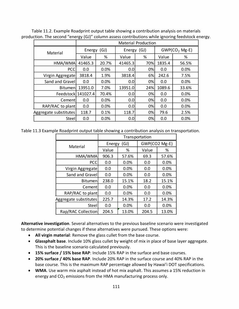
111

Table 11.2. Example Roadprint output table showing a contribution analysis on materials production. The second “energy (GJ)” column assess contributions while ignoring feedstock energy.

Table 11.3 Example Roadprint output table showing a contribution analysis on transportation.

Alternative investigation. Several alternatives to the previous baseline scenario were investigated to determine potential changes if these alternatives were pursued. These options were:

All virgin material: Remove the glass cullet from the base course.

Glassphalt base. Include 10% glass cullet by weight of mix in place of base layer aggregate. This is the baseline scenario calculated previously.

15% surface / 15% base RAP: Include 15% RAP in the surface and base courses.

20% surface / 40% base RAP. Include 20% RAP in the surface course and 40% RAP in the base course. This is the maximum RAP percentage allowed by Hawai’i DOT specifications.

WMA. Use warm mix asphalt instead of hot mix asphalt. This assumes a 15% reduction in energy and CO2 emissions from the HMA manufacturing process only.

Value % Value % Value %

HMA/WMA 41465.3 20.7% 41465.3 70% 1835.4 56.5%

PCC 0.0 0.0% 0.0 0% 0.0 0.0%

Virgin Aggregate 3818.4 1.9% 3818.4 6% 242.6 7.5%

Sand and Gravel 0.0 0.0% 0.0 0% 0.0 0.0%

Bitumen 13951.0 7.0% 13951.0 24% 1089.6 33.6%

Feedstock 141027.4 70.4% 0.0 0% 0.0 0.0%

Cement 0.0 0.0% 0.0 0% 0.0 0.0%

RAP/RAC to plant 0.0 0.0% 0.0 0% 0.0 0.0%

Aggregate substitutes 118.7 0.1% 118.7 0% 79.6 2.5%

Steel 0.0 0.0% 0.0 0% 0.0 0.0%

Rap/RAC Collection 0 0% 0 0%

MaterialGWP(CO2 Mg-E)

Material Production

Energy (GJ)Energy (GJ)

Value % Value %

HMA/WMA 906.3 57.6% 69.3 57.6%

PCC 0.0 0.0% 0.0 0.0%

Virgin Aggregate 0.0 0.0% 0.0 0.0%

Sand and Gravel 0.0 0.0% 0.0 0.0%

Bitumen 238.0 15.1% 18.2 15.1%

Cement 0.0 0.0% 0.0 0.0%

RAP/RAC to plant 0.0 0.0% 0.0 0.0%

Aggregate substitutes 225.7 14.3% 17.2 14.3%

Steel 0.0 0.0% 0.0 0.0%

Rap/RAC Collection 204.5 13.0% 204.5 13.0%

Material

Transportation

Energy (GJ) GWP(CO2 Mg-E)

112

SMA. Use a stone matrix asphalt surface course at 6.5% asphalt by total weight of mix that allows a surface life of 17 years. This results in resurfacing at years 17 and 34 only.

Quiet pavement. Use an open-graded friction course to reduce tire-pavement noise. This mix is at 10% asphalt by total weight of mix (20% of the asphalt binder is ground tire rubber) and the surface life is assumed to be 8 years. This results in five total resurfacings during the 50-year analysis period

Ultimate. Use a combination of a SMA surface course, no glass in the base course, 40% RAP in the base course and warm mix asphalt for both courses in order to reduce the energy and greenhouse gas (GHG) footprint to the maximum extent possible given current standards.

Figure 11.5 through 11.6 shows the percentage change from the baseline practice in terms of energy consumption.

Figure 11.3. Life cycle energy consumption for the current practice and eight alternate scenarios for the example LCA.

113

Figure 11.4. Life cycle CO2 equivalent emissions for the current practice and eight alternate scenarios for the example LCA.

Figure 11.5. The percentage change from the baseline value of energy consumption for a number of alternate scenarios for the example LCA.

114

Figure 11.6. The percentage change from the baseline value of CO2e emissions for a number of alternate scenarios for the example LCA. General conclusions. Some general conclusions that can be reached for this example are:

Extending service life can be the biggest single influence in energy used and CO2 emitted by the pavement. The biggest single improvement came with the use of SMA and the assumed increase in surface life from 10 to 17 years.

Often, a combination of options can produce an even greater savings in energy used and CO2 emitted by the pavement. Several of the options can be combined on one project to provide even bigger savings.

The inclusion or exclusion of the glass cullet makes very little difference in energy used and CO2 emitted by the pavement. While the inclusion of glass cullet was, at one time, mandated in Hawai’i (where practical), it inclusion has little impact on energy and emissions.

The use of quiet pavement (and it’s assumed shorter surface life of 8 years) results in the consumption of more materials and a corresponding increase in energy and emissions. Therefore, in this scenario the use of quiet pavement represents a sacrifice in energy and emissions in order to achieve less tire-pavement noise.

11.4 References Athena Institute. (2013). Impact Estimator for Highways: User Guide. Athena Institute, Ottawa, ON.

Lin, Y.Y. (2012). Eco-decision Making for Pavement Construction Projects. Ph.D. dissertation. University of Washington, Seattle, WA.

115

Muench, S.T. (2010). Roadway Construction Sustainability Impacts: A Life Cycle Assessment Review. Transportation Research Record 2151, TRB, National Research Council, Washington, D.C., pp. 36-45.

Mukherjee, A. and Cass, D. (2012). Project Emissions Estimator: Implementation of a Project-Based Framework for Monitoring the Greenhouse Gas Emissions of Pavement. In Transportation Research Record, No. 2282. Transportation Research Board of the National Academies, Washington, D.C. pp. 91-99.

Santero, N. (2009). Pavements and the Environment: A Life-Cycle Assessment Approach. Ph.D. dissertation, University of California, Berkeley. Berkeley, CA.

Sutley, N.H., Chair, Council on Environmental Quality. (18 February 2010). Memorandum for Heads of Federal Departments and Agencies.

Some pavement LCAs Athena Institute. (2006). A Life-Cycle Perspective on Concrete and Asphalt Roadways: Embodied

Primary Energy and Global Warming Potential. Report to the Cement Association of Canada.

Carpenter, A.C., Gardner, K.H., Fopiano, J., Benson, C.H., Edil, T.B.. (2007). Life Cycle based risk assessment of recycled materials in roadway construction. Waste Management 27, pp. 1458-1464.

Chui, C-T., Hsu, T-H., Yang, W-F. (2008). Life cycle assessment on using recycled materials for rehabilitating asphalt pavements. Resources, Conservation and Recycling 52, pp. 545- 556.

Horvath, A. (2003). Life-Cycle Environmental and Economic Assessment of Using Recycled Materials for Asphalt Pavements. University of California Transportation Center, Berkeley, CA.

Huang, Y., Bird, R., Bell, M. (2009). A comparative study of the emissions by road maintenance works and the disrupted traffic using life cycle assessment and micro-simulation. Transportation Research Part D 14, pp. 197-204.

Huang, Y., Bird, R., Heidrich, O. (2009). Development of a life cycle assessment tool for construction and maintenance of asphalt pavements. J. of Cleaner Production 17, 2009, pp. 283-296.

Mroueh, U-M, Eskola, P., Laine-Ylijoki, J. (2001). Life-cycle impacts of the use of industrial by products in road and earth construction. Waste Management 21, 2001, pp. 271-277.

Rajendran, S., Gambatese, J.A. (2005). Solid Waste Generation in Asphalt and Reinforced Concrete Roadway Life Cycles. J. of Infrastructure Systems 13(2), pp. 88-96.

Stripple, H. (2000). Life Cycle Inventory of Asphalt Pavements. IVL Swedish Environmental research Institute Ltd report for the European Asphalt Pavement Association (EAPA) and Eurobitume, 2000.

116

Stripple, H. (2001). Life Cycle Assessment of Road: A Pilot Study for Inventory Analysis, Second Revised Edition. IVL Swedish Environmental Research Institute Ltd report for the Swedish National Road Administration.

Tramore House Regional Design Office. (2006). Integration of the Measurement of Energy Usage into Road Design. Final Report to the Commission of the European Directorate-General for Energy and Transport. Project Number 4.1031/Z/02-091/2002, 2006.

Treloar, G.J.; Love, P.E.D. and Crawford, R.H. (2004). Hybrid Life-Cycle Inventory for Road Construction and Use, J. of Const. Engr. and Mgmt. 130(1), pp. 43-49.

Weiland, C.D. Life Cycle Assessment of Portland Cement Concrete Interstate Highway Rehabilitation and Replacement. Master’s Thesis, University of Washington, Seattle, WA, 2008.

Zapata, P., Gambatese, J.A., (2005). Energy Consumption of Asphalt and Reinforced Concrete Pavement Materials and Construction. J. of Infrastructure Systems 11(1), pp. 9-20.

117

Section 12 Miscellaneous Material Properties

12.1 Purpose This section provides summaries of material properties that are relevant in designing pavement renewal options.

12.2 Material Properties Table 12.1 shows typical layer moduli for several material conditions. Table 12.2 shows information about rubblized PCC and Table 12.3 about crack and seat renewal.

Table 12.1 HMA Pavement Typical Moduli and Ranges of Moduli

Material Modulus Range (psi)

HMA (temperature dependent) 50,000 to 4,000,000

Cracked HMA Range 50,000 to 500,000

Cracked HMA (10% of wheelpath—slight to moderate fatigue cracks)

100,000 to 250,000

Pulverized HMA 40,000

Table 12.2 PCC Pavement Rubblization Typical Moduli and Ranges of Moduli

Material Value or Property

Ratio of rubblized PCC elastic modulus/original PCC slab elastic modulus

0.05

Slab modulus range prior to rubblization Range: 3,000,000 to 7,000,000 psi

Typical slab modulus 4,000,000

Rubblized PCC Modulus Range: 40,000 to 700,000 psi

Typical Rubblized PCC Modulus 50,000 to 150,000 psi

Table 12.3 Crack and Seat and Break and Seat Renewal

Material Value or Property

Typical modulus of crack and seated PCCP 200,000 psi

Modulus of crack and seated PCCP Range: 200,000 to 800,000

Modulus of break and seat PCCP Range: 250,000 to 2,000,000 psi

118

12.3 References Buncher, M., Fitts, G., Scullion, T., and McQueen, R. (2008), “Development of Guidelines for Rubblization—Final Report,” Airfield Asphalt Pavement Technology Program Project 04-01, Asphalt Institute, May 2008.

Sebesta, S. and Scullion, T. (2007), “Field Evaluations and Guidelines for Rubblization in Texas,” Report No. FHWA/TX-08/0-4687-2, Texas Transportation Institute, December 2007.