profit maximization with bankruptcy and variable...

ELSEVIER Journal of Economic Dynamics and Control

22 (1998) 849-867

Profit maximization with bankruptcy and variable scale

Roy Radner

Stern School of Business, MEC 9-68, New York University, 44 West 4th Street, NY 10012, USA

Received 13 February 1997; accepted 7 July 1997

Abstract

In a diffusion model of an enterprise with variable scale, conditions are given for the maximization of ‘profit’ (expected total discounted withdrawals) to lead to bankruptcy almost surely. The optimal withdrawal policy is an ‘overflow policy’: the withdrawal rate is zero if the asset level is below a ‘barrier’, and equal to the maximum rate if the asset level is at least equal to the barrier. The optimal policy for the control of the drift (yield) and volatility (risk) of the earnings is the solution of an explicit differential equation, and a formula is given for the corresponding value function. @ 1998 Elsevier Science B.V. All rights reserved.

JEL classification: D21; G33; L2

Keywords: Bankruptcy; Profit maximization; Uncertainty; Corporate finance

1. Introduction

In models of an enterprise with ‘fixed productive capacity’, Dutta and Radner (1993), and Radner and Shepp (1996), have shown that the maximization of ‘profit’, i.e., expected total discounted withdrawals from cash reserves (retained earnings), leads to eventual bankruptcy with probability one. In these notes I generalize these results to a model of a firm with variable scale.

As in the papers cited above, the asset level of the enterprise is modelled as a controlled diffusion process. The earnings process is a diffusion whose drift and volatility are controlled by the economic agent (owner, entrepreneur, and/or

This paper is based on research supported in part by a summer research grant from the Leonard

N. Stem School of Business, New York University. I thank Amy Radunskaya, Panagiotis Paraskevo-

poulos, Hsueh-Ling ,Hujnh, Prajit K. Dutta, and Peter B. Linhart for helpful discussions on this topic.

01651889/5%/$19.00 0 1998 Elsevier Science B.V. All rights reserved

PII SO165-1889(97)00090-O

850 R. RadnerlJournal of Economic Dynamics and Control 22 (1998) 849-867

manager) within a prescribed constraint set that depends on the current level of assets (the ‘scale’ of the enterprise). Earnings may be retained and reinvested, thus increasing the asset level, or withdrawn and paid to investors, or divided between the two. The enterprise ‘fails’ the first time (if ever) that the asset level, net of sunk costs, falls to zero. ‘Profit’ is defined to be the expected total discounted withdrawals.

For any current level of assets y, let A(y) denote the corresponding set of feasible drift-volatility pairs. The set-valued function A represents the ‘earnings technology’ available to the agent. I make assumptions about A that express limits on the returns to scale of this technology, and also guarantee that it is mathematically well behaved. For example, it is known that in the case of constant or increasing returns to scale (suitably defined), the maximum profit is either infinite or zero; hence, I limit my model to a case of decreasing returns to scale. However, scale affects both drift and volatility, so the definition of ‘decreasing returns’ adopted here is more complex than it would be in the case of certainty.

With these assumptions, I show that the optimal withdrawal policy is what Dutta and Radner (1993) call an ‘overflow policy’, in which, for some suitably chosen parameter b, the barrier, the withdrawal rate is zero if the asset level is below b, and equals the maximum permissible otherwise. I deal separately with the two cases in which (1) the admissible rates of withdrawal per unit time are bounded above, and (2) the admissible withdrawal rates are unbounded. I also characterize (in each case) the optimal earnings control policy as the solution of an ordinary differential equation, and give a formula for the maximum profit (as a function of the initial asset level) in terms of the optimal earnings control function. For asset levels below the barrier, b, the optimal drift and volatility of earnings are both increasing functions of the asset level.

In the unbounded-withdrawals case, the optimal drift of earnings at the level of the barrier is equal to the maximum possible for that level of assets. In this case, if the asset level starts at or below the barrier, it never rises above it; whereas if it starts above the barrier then it jumps down (discontinuously) to the barrier and never rises above it again. As a consequence, the enterprise will fail in finite time, almost surely.

In the bounded-withdrawals case, the asset level may drift above the barrier. If the maximum rate of withdrawal exceeds the maximum drift of earnings, then the asset level will eventually return to the barrier; as a consequence, the enterprise will again eventually fail in finite time. On the other hand, if the earnings drift exceeds the withdrawal rate, then there is a positive probability that the enterprise will never fail. For example, for a fixed withdrawal rate, if the eam- ings drift is unbounded as the asset level increases without bound, then there will be a critical asset level, say y*, such that, conditional on the asset level reaching y*, the probability that the enterprise never fails is positive. However, given the initial asset level, the probability of surviving forever ten& to zero as the withdrawal rate increases without bound.

R. Radner I Journal of Economic Dynamics and Comrol22 (I 998) 849-867 851

Sections 2 and 3 are devoted to the bounded-withdrawals case. In Section 2,

I present the formal model and outline the method of proof. In Section 3,

I present the assumptions, and state and prove the main result. A special case (‘multiplicative scaling’) is analyzed in Section 4, where the notion of decreasing returns to scale is given a more intuitive representation. The unbounded- withdrawals case is discussed in Section 5, where the notion of an overflow

withdrawal policy is made precise, and it is shown that the supremum of the profit when all finite withdrawal rates are allowed is attained by such a policy.

The failure times for both the bounded- and unbounded-withdrawals cases are

discussed in Section 6.

Essential references are listed in the final section. Additional references, and a full discussion of the topic of profit maximization and market selection, will be

found in Dutta and Radner (1993). A summary of related results on economic survival will be found in Radner (1996).

2. A general model of variable scale

Let Y(t) denote the assets of the enterprise at time t (not counting sunk costs). I shall assume, unless it is mentioned to the contrary, that the initial asset level,

Y(O), is strictly positive. The agent (entrepreneur, manager) controls two vari-

ables, u(t) and w(t), where u(t) controls the drift and volatility of the (net) earnings process at time t and w(t) is the instantaneous rate of withdrawal at time t (see end of Section 3 for comments on this formulation). The asset process Y(t), is a diffusion with

drift = m[u(t), Y(t)] - w(t),

volatility = u[u(t), Y(t)].

Call the function u the earnings control; assume that it takes its values in the unit interval [0, 11. Also, call the function w the withdrawal control; assume that

it takes its values in the closed interval [0, w*], where w* is a positive parameter. (I shall usually think of w* as being ‘very large’.) Note that it is implicit in the above description of the asset process, Y(t), that at time t the earnings process has drift m[u(t), Y(t)] and volatility u[u(t), Y(t)].

(Note: The underlying earnings process is a diffusion that is adapted to some filtration. The controls u and w must be adapted to the same filtration. Further- more, the controls are required to be measurable with respect to the time variable,

t>O.) Let T be defined by

T=inf{t: Y(t)=O}.

852 R. RadnerIJournal of Economic Dynamics and Control 22 (1998) 849-867

Call the random variable T the failure time; it could be infinite. I shall say that the enterprise survives (forever) if T is infinite; otherwise the enterprise fails.

The enterprise’s (expected) profit is defined to be

J T

P=E e-“w(t) dt, 0

where r > 0 is an (exogenously given) interest rate. The controls u and w are optimal if they maximize profit. Correspondingly, let P(y) denote the maximum profit, given that Y(0) = y.

In what follows, I shall present assumptions sufficient to guarantee the existence of optimal controls. Under these same assumptions, I shall show that the optimal withdrawal policy, w, has the following form, which I call an ‘overflow policy’: the withdrawal equals 0 or w* according as Y(t) is < or 2 b. I shall also ‘construct’ the optimal earnings control as the solution of an ordinary differential equation, and give a formula for the value function, P(y), in terms of the optimal control functions. The optimality of the constructed controls will be demonstrated using the so-called ‘Bellman optimality conditions’ (see, e.g., Krylov, 1980).

In fact, I shall now use the Bellman conditions to motivate the assumptions and the construction of the optimal policy. But first, I note that Blackwell’s theorem will imply that we may take the optimal controls to be ‘stationary’, i.e., for some functions U and W,

u(t) = ~[~(Ol, (1)

w(t) = kV[Y(t)].

Second, I note that a stationary withdrawal policy is an overflow policy if, for some b>O

0 W(Y) =

if y < b,

W* if y2 b. (2)

Suppose that the value function is continuously twice differentiable (which it will be), and define the ‘Bellmanian’ function B of the nonnegative variables u, w,

and Y, by

mGwY)=w - rP(y) + M%Y> - WIP’CY) + v/w~,Y)P”(Y). (3)

The following three conditions (the Bellman conditions) will be sufiicient for U and W to be optimal:

P is C2. (4)

For every Y > 0, NWY), WY>, rl = 0. (5)

For every y > 0, u in [0, 11, and w in [0, w*], B(u,w, y) 5 0. (6)

R. RadnerlJournal of Economic Dynamics and Control 22 (1998) 849-867 853

In the presence of (S), condition (6) is equivalent to

For every y > 0, [U(y), W(y)] maximizes B(u, w, y). (7)

One can rewrite the Bellmanian (3) as follows:

B(u,w, y) = w[l - P’(y)1 - rP(y) + MC% YV(Y> + VPM% YV’(Y).

From this we see that the overflow withdrawal policy (2) satisfies the maximization condition (7) provided

P'(Y) {

>I if y <b,

< 1 if y > b. 03)

In fact, I shall show that

P’ > 0, PII < 0,

so that it will be sufficient for b to satisfy

P’(b) = 1.

(9)

With regard to the earnings control, U, suppose that it satisfies the first-order

condition for the maximization of the Bellmanian (3); then

ml[U(v),~lP’(~)+ (1/2)~1[u(y),ylP"t~)=O. (10)

Eqs. (5) and (10) imply that, where u1 > 0,

WY) - WY) + w-J(Y), Yl - VY))P’CY) = 0, (11)

where

(12)

Differentiating (11) with respect to y, and bearing (2) in mind, we obtain, for

Y#k

t-r + Sl[VY),YlU’(Y) + S2[~(Y),Yl~P’(Y)

+ MU(Y )T Yl - W(Y M”(Y)

=o. (13)

Eqs. (10) and (13), together with P’ > 0 [cf. Eq. (9)], imply, for y # b, that

Sl[U(Y),YlU’CY) -r+S2KJCYLYl- {SKJ(Y),Yl- uY))H(Y)=O, (14)

where

fwY)- 2mdu, y)

u*(u y) -

,

(15)


Suppose that gi > 0; then (14) can be solved to for U’(y) to give, for y # b:

U’(Y) = ~[~(Y),YlMWY)~Yl - WY)) - g2W(Y),Yl+ r

91 [WY), Yl (16)

Note that this differential equation in U does not involve the unknown value function, P. For a reason that will become apparent below, I impose the boundary condition:

u(o) = uo(O), (17)

where, for each y,

M4 Y> us(y) maximizes ___ u(u, Y)

(the existence of us(y) will be guaranteed by the assumptions). Thus far, I have sketched how to construct the optimal controls, provided

suitable assumptions are made on the functions m and u. I shall now show how, given the controls, to calculate the value function, P. From (10) and (15) we have

P”(v)= -UJ(Y)9YlP’(Y).

A solution of this is

(1%

{J Y

P’(y) = exp - b

(20)

Integrating this last, and taking the constant of integration to be 0, we have

J Y

P(Y) = P’(x) dx. (21) 0

Note that

P(0) = 0, P’(Y) > 0, P’(b) = 1. (22)

Suppose that, for each y, the function m(u, y) has a unique maximum in u at the point u*(y), interior to the unit interval. From (10) and (22) we see that P”(y) < 0 iff U(y) _< u*(y). Hence, we shall have constructed an optimal policy if we can find a value of the barrier b, such that the solution to the differential equation (16), with boundary condition (17), satisfies, for all y,

0 < WY) i U’(Y). (23)

In the next section, I show how this can be done, under suitable assumptions about the data of the problem, namely the functions m and u, and the parameters r and w*.

R. RadnerlJournal of Economic Dynamics and Control 22 (1998) 849367 855

3. Assumptions and main result

In this section, I shall carry out the program outlined in Section 2, by stating

a set of assumptions, and stating and proving the main result. I shall call the level of assets, Y(t), the scale of the enterprise at time t.

The first set of assumptions describes how the drift and volatility of earnings vary with the control variable, U, for each scale y. In particular, they assure that

the problem is mathematically well-behaved (see end of this section for further comments).

Assumption Al. (1) m and u are C2 on [0, l] x [O,oo). For each scale y, consider m and o as functions of u.

(2) m is strictly positive and strictly concave. (3) u is strictly increasing and (weakly) convex, and u and ui are positive and

bounded away from 0. (4) For every y, the maximum drift,

m*(y) = max{m(,, y): u in [0, l]},

is attained at a unique point u*(y), and

(24)

0 <u*(y) < 1, (25)

u* is continuous and nonincreasing. (26)

(5) The ratio 111(u, y)/u(u, y) attains a maximum at a unique point, say ue(y), such that

0 < Uo(Y> <u*(Y) < 1; (27)

Let C denote the closed ‘strip’ of points (u, y) such that y 2 0 and 0 5 u <

u*(y). It follows from Assumption Al that, in C, the ratio mi(u, y)/ui(u, y) is strictly decreasing in u.

From the definition of g, one calculates its partial derivative with respect to u to be

91 = U(~IUIl -m11u1) >. in c

(VI I2 (the positivity of gi in C follows from Assumption Al). Note also that

g[uo(y)l = 0, (29)

and

g[u’(y)l= m*(Y). (30)

856 R. Radnet I Journal of Economic Dynamics and Conrrol22 (1998) 849-867

With Assumption Al we can now justify all of the calculations of Section 2 except for the analysis of the differential equation (16) for the optimal earnings control, U. For the latter, we need some further assumptions.

The next assumption expresses a limit on ‘returns to scale’. The intuitive interpretation of the particular form of this assumption will become clearer in the next section. Note that the assumption places a condition on both the drift and volatility functions.

Assumption A2. Y - gz(u, y) is strictly positive and bounded away from zero in C.

The final assumption expresses the condition that the parameter w* be ‘sufficiently large’; it also implicitly places a further limit on returns to scale.

Assumption A3. For all y > 0, and all u 5 uo(y), H(u, y)w* + gz(u, y) - Y is strictly positive.

I turn now to the analysis of the differential equation (16) on the strip C. It will be convenient to define the two functions,

F(u, Y) = H(u, YMU, Y) - 92t4 Y) + r

Sl(UY Y) ,

G(u

9

y) = fJ(% Y)[dU, Y) - w*1 - 92tu> Y> + r at4 Y>

(31)

With this notation, we can write the differential equation (16) in two parts as

U’(y)=F[U(y), y] for 0 < y <b; (33)

U’~Y>=GW(Y),YI for v>b.

We also have the two boundary conditions,

(34)

W) = uow, (35)

U(b+) = U(b-). (36)

First, I shall show that in the first regime (y < b), the solution U(y) is increasing, and, in fact, would eventually reach u*(y) if b were large enough; call this ‘Curve 1’. Second, considering the differential equation in the second regime to be defined for all y > 0, I shall show that there is a solution, U(y), for some initial value, U(O), that remains in the interval, 0 < U(y) < u*, for all y > 0; call this ‘Curve 2’. The optimal value of b is then the value of y at which Curve 1 (first) crosses Curve. 2.

R. RadnerI Journal of Economic Dynamics and Conrrol22 (1998) 849467 857

Concerning the first regime, first note that g(u,y) > 0 for u > Q(Y), and

H(u,y) > 0 for u < u*(y). Hence, by Assumptions 1 and 2, F(u,y) > 0 (and

is in fact bounded away from 0) for #o(y) < u 5 u*(y). Furthermore,

u;(y) = _ 92[wdY), Yl

91 [UO(Y), Yl < F[UO(Y)> Yl. (37)

Hence, the solution to the first regime remains above Q(Y), is strictly increasing, and eventually reaches u * (y) at some finite y.

Concerning the second regime (without regard to the boundary condition (17)), first note that, from (37) and Assumption A3,

U;(Y) > G[~o(Y), ~1, (38)

and G(u, y) < 0 for u 5 uc(y). Hence, for any initial condition U(0) 5 uo(0), the solution to the second regime is strictly decreasing, and will eventually reach 0 at some finite y. On the other hand, H[u*(y), y] = 0, so that

G[~*(Y)>Y~ = -92[u*(Y),Yl+ ?- > 0

sl[u*(Y),Yl (39)

(the last inequality by Assumption A2). Hence, for some number E > 0, if u*(O)- E 5 U(0) 5 u*(O), then the solution to the second regime will be strictly increas-

ing, and will reach u*(y) at some finite y. Continuing with the analysis of the second regime, fix x > 0. For each initial

value U(0) = U, one of two things can happen: (1) The solution, U(y), reaches the lower boundary of C, U(y) = 0, or the

upper boundary, U(y) = u*(y), at some y < x; in this case set X(u) = y. (2) For all y <x, 0 < U(y) <u*(y), and hence 0 5 U(x) < u*(x); in this

case set X(u) =x. Still fixing x, define the mapping, C,, by C,(u) = { U[X(u)], X(u)}. Define

z(x) to be the ‘truncation’ of z at x, i.e., the subset of C for which y 5 x. From the previous paragraph, we see that the mapping C, takes its values only in the upper, lower, and right boundary of C(x).

Lemma 1. For each x, the mapping C, is continuous from the interval [O,u*(O)] to C(x).

(Lemma 1 can be derived using the Wasewski’s theorem (Hartman, 1982, pp. 280 ff.). However, see Appendix A for a self-contained proof.)

Let D(x) denote the (closed) interval, [O,u*(x)] x {x}, i.e., the right boundary of C(x), and let Z(x) denote the set of initial values u such that C,.(u) is in D(x). In other words, Z(x) is the set of initial values for the second regime such that the solution does not reach 0 or u*(y) before y reaches x. For u < Q(O), C,(u) is in the lower boundary of z(x), whereas for u sufficiently close to u*(O), C,(u)

858 R. Radner I Journal of Economic Dynamics and Control 22 (1998) 849-867

is in the upper boundary. Since C, is continuous, there exists a u such that C, is in D(X), so that I(x) is not empty.

Now let x increase. For each x, the set Z(x) is a nonempty closed subset of [0, u*(O)], and X’ > x implies I@‘) 2 Z(x). Hence, by the Heine-Bore1 theorem there exists some u2 that is in Z(x) for every x > 0. Furthermore, uz > ua(0) (here we use, in particular, Assumption A3).

We can now determine the optimal barrier, b. Let Vi denote the solution to the first regime (33), subject to the boundary condition, Vi(O) =uo(O), and let U2 denote the solution to the second regime (34), subject to the boundary condition, Q(O) = ~2. Note that, by the choice of uz,

05 U~(Y)IU*(Y), for Y>O. (40)

Let b be smallest solution to the equation,

Q(b) = G(b), (41)

and define U by

U(Y) = vi(v) or Q(Y) as y < or >b. (42)

The function U satisfies the differential equation (16)-( 17), and the condition (23), and hence is an optimal control. Hence, I have proved:

Theorem I. Under Assumptions Al-A3, the earnings control U defined by (42), together with the withdrawal control W dejned by (2), are optimal, and the optimal profit function, P, is given by (20)-(21).

I conclude the section with some comments about Assumptions Al and A2. Perhaps a more natural formulation of the model would have started with assumptions about the sets A(y) of feasible drift-volatility pairs for each scale y. For example, following Dutta and Radner (1993), I might have assumed that A(y) is a compact, convex set, with smooth boundary, in which (1) there is a point with positive drift, and (2) there is no point with zero volatility. Anticipating that the optimal value function, P, will be strictly increasing in the scale, y, we infer from the Bellmanian function (3) that, for each scale y, the drift will be the maximum possible in A(y), given the optimal volatility. Hence, we could parametrize the control by the volatility, v. However, the range of v varies with the scale y, so it is more convenient to parametrize the control by some variable u that has a fixed range, say the unit interval, and is a strictly increasing function of v for each scale. For example, let v’(y) > 0 be the minimum value of v for (m, v) in A(y), let v”(y) be the maximum value, and let u = [v - v’(y)]/[v” -v’(y)]. Solving this for v Yields a function, v(u, y), and setting the drift equal to the maximum given v and y yields a function, m(u, y). However, other parametrizations are possible; for example, by making 1( a suitable nonlinear function of v, one could force the function u*(y) to be a constant.

R. Radneri Journal of Economic Dynamics and Control 22 (1998) 849-867 859

4. Example: Multiplicative scaling

Suppose that the drift and volatility functions take the form

m(u, Y) = M(n)WY)> (43)

u(u, Y) = V(U)%Y). (44)

I shall call this the ‘multiplicative scaling model’. Corresponding to Assumption 1

of Section 3, I assume:

Assumption IMS. (1) M and V are C2 on [0, 11; R and S are C2 on [O,co). (2) On (0, 1 ), it4 is strictly positive and strictly concave, and M(u) attains its

maximum at a (unique) point u* such that

o<l.i*<1. (45)

(3) On [0, 11, V is strictly increasing and (weakly) convex, and V and V’ are

positive and bounded away from 0. (4) R and S are strictly positive, and nondecreasing (and hence bounded away

from zero). (5) The ratio M(u)/V(u) attains a maximum at a unique point uo such that

o<ua<u*.

Let

k(u)-M(u) - V(u) M$J ; [ I (46)

du, Y) = k(u)R(~),

sdu,y)=k’WR(~)>

gz(uv y> = WR’(y).

Note also that ug and u* are independent of y, and satisfy

k(uo) = 0, M’(u’) = 0.

Furthermore,

k, = V( V”M’ - V’M”)

(V’)2 ’

(47)

(48)

(49)

(50)

(51)

k(u) <0 if u < ua,

>O ifu>uo, (52)


k(u*)=M(u*).

Define

h(u) ZZ 2M’(u)/Y’(u);

then

(53)

(54)

and

fJ(% Y> =Mu)[NYYS(Y)l, (55)

F(u, Y) 3 ~(~)[NY)/S(Y)l~(U)~(Y) - MU)R’(Y) + r

k’(U)R(Y) , (56)

G(u,y)= Nn)[R(Y)/S(Y)l[k(u)NY) - w*1- k(U)R’(Y) + r.

k’(U)R(Y) , (57)

the differential equation for the optimal earnings control U can again be written in the form (33)-(34).

Corresponding to Assumption A2 of Section 3, I assume:

Assumption A2MS. R is concave, S is convex, and

M(u*)R’(O) < r. (58)

This assumption is clearly interpretable as a limit on returns to scale. Since k is increasing, k(u*) =M(u* ), and R’ is nonincreasing, it follows that, for all u 5 U* and y>O,

- k(u)R’(y) + r > 0,

so that Assumption A2 is satisfied.

(59)

Corresponding to Assumption A3 we have:

Assumption A3MS. For all u < uo and y > 0,

h(u)[R(y)/S(y)lw* + W)R’(y) - r ’ 0. (60)

Again, this expresses the assumption that w* is ‘large enough’, but also places a further limit on returns to scale. This form brings out more clearly than does Assumption A3 that the limitation on returns to scale involves the volatility as well as the drift. For example, it would not be unusual for R’(y) to approach 0 as y gets large (‘decreasing returns to scale’), in which case the assumption requires that the ratio R(y)/?(y) be bounded away from zero. This would be the case, for example, if both R(y) and S(y) approached limits as y became large (‘bounded scale’).

If both R and S are independent of y, we might say that the enterprise has ‘constant size’. (This was the case treated in Dutta and Radner (1993) and Radner

R. Radner I Journal of Economic Dynamics and Control 22 (1998) 849-867 861

and Shepp (1996) but by somewhat different methods.) One can verify that, in

this case, the solution U2 in (42) is actually a constant, i.e.,

U,(y) = Q(6) for y > b.

(I omit the details.)

5. Unbounded withdrawals

I now consider the case in which the rate of withdrawal, w(f), is unbounded but finite. We shall see that the supremum of the profit in this case is attained by a policy that is not in this class, but is an overflow policy in which the withdrawal

rate is zero when the asset level is below the barrier b, and ‘infinite’ when it is

above the barrier. (This will be made more precise below.) With such a policy,

the asset level, Y(r), never rises above the barrier, although it may start above the barrier at time zero. As we shall see, with a withdrawal policy of this type, the firm will fail in finite time, almost surely (see Section 6). Optimality will be

proved using a simpler form of Assumption A3. For the optimal policy, at asset levels below the barrier, both the drift and the

volatility will be increasing functions of the asset level, and at the barrier, the drift will equal the maximum possible for Y(t) = b. Since Y(t) will not spend any (positive amount of) time above the barrier, it will not be necessary to specify the optimal control of earnings in that region.

To define the overtlow policy, it is convenient to denote the underlying cumulative earnings process by X(t). The drift, m(t), and the volatility, o(t), of the cumulative earnings process are controlled through the control variable, u(t), as

in Section 2, and X(0) = 0. Let Q(t) denote the cumulative withdrawals up to time t. In the case of a policy with a finite withdrawal rate, w(t), the cumulative withdrawal is defined by

f sqt) =

J w(s) ds. (62)

0

The asset level at time t is defined by

Y(t) = Y(0) +x(t) - Q(O

I shall define the overflow policy with barrier b by

Q*(t) = sup{[Y(O) +X(s) - b]+ IO 5s 5 t},

(63)

(64)

where for any number z, z+ = max{z, 0). (For a discussion of this type of policy, see Harrison, 1985, pp. 19 ff.) As noted above, if Y(O)< b, then Y(t)< b for all t 10, whereas if Y(0) > b, then Q*(O) = Y(0) - b, Y(O+) = b, and Y(t) 2 b for

862 R. Radnerl Journal of Economic Dynamics and Control 22 (1998) 849-867

all t > 0. Thus, if Y(0) > b, then Y has a downward jump of Y(0) - b at time 0. I note that the overflow policy with barrier b is a stationary policy.

Since the asset level, Y(t), never exceeds b for t > 0, the optimal control corresponding to the overflow policy with barrier b need be defined only for Y(t) 5 b. This (optimal) control will be determined by the differential equation,

U’(Y) = QW), ~1 for 0 < Y < 4 (65)

U(O) = uo(O), (66)

where the function F is given by Eq. (31 in Section 3. The optimal barrier b, will be the smallest number b that satisfies

U(b) = u*(b). (67)

Hence, U(y) is strictly increasing for 0 < y < b. Let a(oo) denote the overflow policy with barrier b just described, and let P

denote its corresponding profit function. It is clear that for y > b,

P(y) =P(b) + y - b. (68)

For y < b, the profit function P is determined by Eqs. (19)-(21) of Section 3, together with

P(b) = ;ib P(Y ),

y<b

(69)

and hence (22) is satisfied. Furthermore, note that, since H[u*(y), y] = 0, it follows that P”(b) = 0, so that P is C2.

I now replace Assumption A3 of Section 3 with:

Assumption A3*.

Am*(y) <r dy

for y > b. (70)

Theorem 2. Under Assumptions Al, A2, and A3’, the supremum of profit for unbounded withdrawal rates is given by the profit function P defined above, with the corresponding control U, and the overJlow policy with barrier b determined by Eq. (67).

(Note: For Theorem 2, we need only the assumption that u* be continuous, but not that it be nonincreasing as in Assumption A1(4).)

Proof: By construction of the control U, the Bellman optimality conditions are satisfied for y 5 b, just as in the proof of Theorem 1 of Section 3. For y > b,

R. RadneriJournal of Economic Dynamics and Control 22 (1998) 849-867 863

we have P’(y) = 1, P”(y) = 0, and hence the Bellmanian function (see (3)) is

given by

B = W - rP(y) + [m(u, y) - WI

= -r[P(b) + y - b] + m(u, y)

I -r[P(b) + y - b] + m”(y). (71)

I first want to show that the profit function P majorizes the profit from any policy with a bounded withdrawal. For this it suffices to show that the Bellmanian

corresponding to the profit function P is nonpositive. From (3), (5), (67), and

(69),

- r-P(b) + m*(b) = 0, (72)

and, hence,

B 5 - m*(b) + r(y - b) + m*(y). (73)

But by (70), for y > b,

M*(Y) < m*(b) + 4~ - b), (74)

and so B 5 0. It remains to ,show that the profit function P can be approximated arbitrarily

well by bounded-withdrawal policies. As above, let b be the optimal barrier for the unbounded case. Fix w > 0, and define the bounded-withdrawal policy W(y; w) by (2), with w* replace by w. Let the earnings control be that for the

unbounded case, for y <b, and equal to u*(y) for y 2 b. Call the combined policy x(w), and let P(y; w) denote the corresponding profit function. I shall show that

?$a P(Y; w) = P(Y). (75)

Since the policy rc(w) coincides with the unbounded-withdrawal policy x(00) for y I b, I first consider the case y > b. The profit function P(y; w) satisfies the differential equation,

w - rP(y; w) + [M(y) - w]P’(y; w) + (1/2)V(y)P”(Y; w) = 0, (76)

where M(y) and V(y) are the drift and volatility functions prescribed by the policy X(W), and P’, P” denote derivatives with respect to the variable y. Dividing this last by w, we get,

MY) 1 - (r/w)P(y;w) + - -

[ 1 W 1 P’(y;w)+

V(Y) FP”(y; w) = 0. (77)

864 R. Radnerl Journal of Economic Dynamics and Control 22 (1998) 849-867

Letting w -3 oo, we get

lim P’(y; w) = 1. W-M

For y < b, the policies X(W) and rc(co) coincide; furthermore,

P’(b-; w) =P’(b+; w).

Hence, for all y,

&nm P’(y; w) = P’(y).

In addition,

P(b-; w) = P(b+; w),

so that

Jew P(Y; w> = P(Y),

(78)

(79)

(80)

(81)

(82)

which completes the proof of Theorem 2. 0

6. Failure

In the case of unbounded withdrawals (see the preceding section), the enterprise will almost surely fail in finite time (T < co); in fact, the expected time to failure is finite (see, e.g., Harrison, 1985, p. 87).

The case of bounded withdrawals is more complex. In the special case of ‘constant size’ (see the end of Section 4), the enterprise will almost surely fail in finite time provided that w* is large enough; for example, it suffices that w* >M(u*), which in turn implies that the drift of the asset level, Y(t), is strictly negative whenever Y(t) > b. Roughly speaking, whenever Y(t) is above the barrier b, it will eventually return to the interval [0, b], and whenever it is in that interval there is a positive probability that it will reach 0. Hence, Y(t) will eventually reach 0.

In the more general case of variable scale, the drift can increase with the asset level. For example, consider the multiplicative scaling model of Section 4, and assume that:

(1) the scale function R is increasing and unbounded, whereas S is independent of scale;

(2) the minimum of M(u) on [0, l] is strictly positive.

If follows that for any (finite) w* and any barrier b there is a scale y* > b such that, for any control function U, for all Y(t) 2 y*, the drift of Y(f) will be positive and bounded away from zero. In this case (since the volatility is bounded

R. RadnerlJournal of Economic Dynamics and Control 22 (1998) 849-867 865

and bounded away from zero), the conditional probability that the enterprise never

fails, given that Y(0) 2 y*, is strictly positive.

In other words, at a large enough scale, the expected rate of earnings (per unit time) of the enterprise is greater than the maximum rate of withdrawal. On the other hand, the larger w* is the larger will be the critical level y*, and the smaller will be the probability that the enterprise will never fail (T = 00). (I omit the details.)

Appendix A

Proof of the Lemma 1. Fix x throughout the proof. There is a bounded set, say C’, which is open in R+ x R, contains the strip Z(x), and in which the function

G in (32) is C2. Let J be the open interval of points u such that (0,~) is in Z’. The differential equation (34) for the second regime has a solution for all initial conditions u in J, and by the ‘continuity theorem’ this solution is continuous in the sup-norm topology, as a function of the initial condition (see, e.g., Arnold, 1973, p. 221, Corollary 31.8). In other words, for any initial condition u in J, let U be the corresponding solution of the differential equation (34) with U(0) = U;

then for any E > 0 there exists an E’ > 0 such that, if u’ E J, with

U - El < 24’ < U + E’, (A.11

and V’ is the solution of (34) with initial condition u’, then for all [y, V(y)] in .??,

I UY> - WY)1 I E. 64.2)

I shall consider four cases: Case 1: C,(U) is in the upper boundary of C(x), and X(u) E y* < x. In this

case,

w?u)l = WY*) = U*(Y*), (A-3)

U’( y* ) > 0. (A.4)

(the latter by (39)). For some nonempty interval K centered on y’, there is a y > 0 such that U’(y) > y for all y in K. Let

y,-y*- f ) 0 y2- y* + E ;

0 Y

tA.5)

tfw

then for E sufficiently small, y1 and y2 are in K, and

~~Yl~+~I~~Y*~-~~y*-Yl~+~=u*~y*), (A.7)

866 R. Radner I Journal of Economic Dynamics and Control 22 (1998) 849-867

I I I

Y’ *

Yt Yl

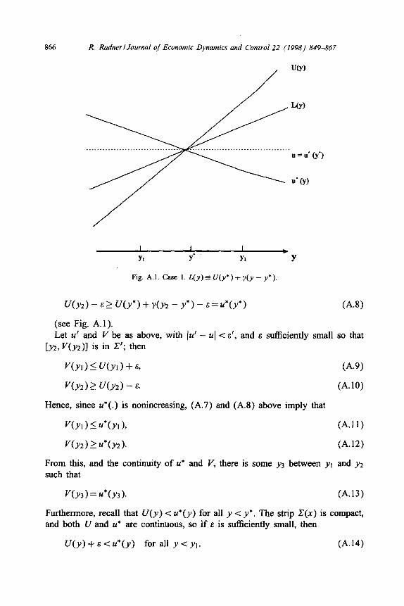
Fig. A.l. Case 1. L(y)~U(y*)+y(y-y*).

Y

64.8)

(see Fig. A.l). Let u’ and V be as above, with (u’ - UJ < E’, and E sufficiently small so that

[y2, Y(y2)] is in Z’; then

V(y1) 5 U(y1) + s, (A.9)

UY2 I> WY2 > - 8. (A.lO)

Hence, since u*(.) is nonincreasing, (A.7) and (A.8) above imply that

V(Yl) I u*cy1>, (A.11)

vY2)zu*(Y2). (A.12)

From this, and the continuity of u* and V, there is some y3 between yt and y2 such that

un>=U*(Y3). (A.13)

Furthermore, recall that U(y) < u*(y) for all y < y*. The strip Z(x) is compact, and both U and u* are continuous, so if E is sticiently small, then

U(y) + 8 -c u*(y) for all y < yt. (A. 14)

R. Radner I Journal of Economic Dynamics and Control 22 (1998) 849-867 861

Hence,

V(y) < u*(y) for all y < yl. (A.15)

First, from (A.13) and (A.14),

Yl I X(0 I y2; (A.16)

hence, by (A.5) and (A.6), we can make (X(u’) --X(u)\ = IX(u’) - y*\ as small

as we like by taking E sufficiently small. Second, note that

I wf(u’)l - wvu)ll 2 I W(~‘)l - ww’)ll

+ IW~(~‘)l - wau))ll. (A.17)

By (A.2), the first term in the right-hand side of the above does not exceed a, whereas by the continuity of U, we can make the second term as small as we

like by making IX(u’) - y* I sufficiently small. Hence, we can make the left-hand side as small as we like by taking E sufficiently small. This completes the proof that, in Case 1, C, is continuous at U.

Case 2: C,(U) is in the lower boundary of C(x), and X(u) <x. In this case use an argument symmetric to that of Case 1, with u*(.) replaced by the constant function, u = 0 (recall that G(0, y) < 0).

Case 3: C,(u) is in the interior of the right-hand boundary, D(x), of I(x), i.e.,

X(u) =x, (A.18)

0 < U(x) < u’(x). (A.19)

In this case, the continuity theorem implies that, for u’ sufficiently close to u

(using the notation of Case 1), V(x) is also in the interior of D(x), and hence, C, is continuous at u.

Case 4: C,(u) is at one of the endpoints of D(x). In this case one combines the arguments of Cases 1 (or 2) and 3. I omit the details.

This completes the proof of the lemma. 0

References

Arnold, V.I., 1973. Ordinary Differential Equations. MIT Press, Cambridge, MA. Dutta, P.K., Radner, R., 1993. Profit maximization and the market selection hypothesis. AT&T Bell

Laboratories, unpublished, revised October 1995. Harrison, J.M., 1985. Brownian Motion and Stochastic Flow Systems. Wiley, New York. Hartman, P., 1982. Ordinary Differential Equations. Birkhauser, Boston. Krylov, N., 1980. Controlled Diffusion Processes. Springer, New York. Radner, R., 1996. Economic Survival: Schwartz Memorial Lecture. Northwestern University,

Evanston. Radner, R., Shepp, L.A., 1996. Risk vs. profit potential: a model for corporate strategy. Journal of

Economic Dynamics and Control 20, 1373-1393.

profit maximization with bankruptcy and variable...

Documents