Profit Maximization

Profit Maximizing Assumptions• Firm: Technical unit that produces goods or

services.• Entrepreneur (owner and manager)

– Gains the firm’s profits and suffers losses and has the goal of maximizing profit.

– Transforms inputs (aka factors) into outputs through the technology of the production function.

– Decides how much of each input to use and what quantity to produce.

Realistic?• For this class, we assume corporation’s with

shareholders and boards and executives function like the entrepreneur.– Obviously, managers and executives have other

incentives besides maximizing profit.– But there is a more developed theory of the firm for

corporations that we will not get into.• Profit maximization?

– Libraries and water utilities are strictly non-profit.– Most hospitals claim to be non-profit, but they act

like for-profit hospitals.

Why Firms?• You could ask why even have firms?• Why don’t entrepreneurs outsource

EVERYTHING?• Transactions costs make that infeasible. Or not.

– In the 1870s-1950s vertical integration was the norm (River Rouge plant included a steel mill and processed rubber).

– Since then, outsourcing has been growing.– New communication technology has driven this more

towards the entrepreneur-only model.

Profit• Profit maximization could easily be 1/2 of the

text as we assume firms maximize profit under a host of situations: perfectly competitive, monopoly, price discrimination, oligopoly, monopsony, etc.

• However, the basics are perfect competition (price taker) and monopoly (price setter).

Price Taker vs Price Setter• Profit is TR-TC• Price Taker (competitive firm)

– Treat the price they face as given when choosing quantity

• Price Setter (single price, no strategic behavior)– Price is chosen along with quantity.

• Short and long run options are the same– Short Run, quantity decision includes the shut down option– Long Run, consideration of returns to scale and entry and exit

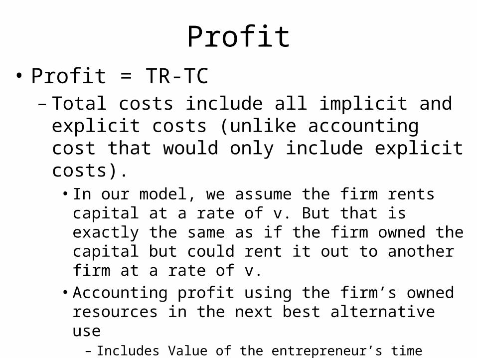
Profit• Profit = TR-TC

– Total costs include all implicit and explicit costs (unlike accounting cost that would only include explicit costs).

• In our model, we assume the firm rents capital at a rate of v. But that is exactly the same as if the firm owned the capital but could rent it out to another firm at a rate of v.

• Accounting profit using the firm’s owned resources in the next best alternative use

– Includes Value of the entrepreneur’s time – Selling off owned factors and investing elsewhere

– For us, SC = VC + FC = wL + vK

Price Takers

• The rest of this lecture focuses on price takers.– Homogeneous output– No barriers to entry/exit in long run– Many sellers– Perfect price information

Revenue: Price Taker• Price Taker

• If a firm charges p > Pm , they will sell q = 0

• Demand for firm’s output is p = Pm, the firm can sell as many as it wants, until q = 3,000,000, and then need to lower the price to sell more.

P

q

Market Demand

1,000 2,000 3,000 3,000,000

p = Pm

However, price taker assumption is that no firm is big enough to be able to affect the market price.

• So for price taker, we assume decreasing returns to scale precludes getting large enough to have production influence price:

• So R = p·q, where p = Pm

Revenue: Price Taker

P

q

Demand for firm:Pm = MR = AR

1,000 5,0003,000

p = Pm

d p q p qMR p, AR p

dq q

Cost and Short Run Supply

CSRC

q

ACSACSMC

q

CSRC

ACSMC

SAC

EhhibitsIRS, DRS

Exhibits IMR, DMR

Exhibits IMR, DMR MC

• Let’s for the moment assume production exhibits IRS and then DRS.• Firms will, in the LR, choose a level of K commensurate with getting the lowest

possible SAC.• The price will be driven to the low point of AC, the break even price.• At this starting point, the firm’s SAC, AVC, and SMC are relevant in the short run• Other returns to scale options considered in the long run.

pbe

AVC

Exhibits IMR, DMR

Cost and Short Run Supply

CSC

q

ACSRACSRMC

q

SC

SMC

SAC

Exhibits IMR, DMR

• But for the moment, we don’t care which level of K the firm has or what the AC curve looks like.

• In the SR, here is what we have to work with.• To determine the profit maximizing level of q = q*, and whether shut down and

produce q = 0, MC and SAVC are most important.

AVC

Exhibits IMR, DMR

Profit Max

SC

q q

R=p·qSC

• Maximize π = R(q) - C(q)• FOC for this yields q where slope of π function = 0

MR=Pslope of R

SMC = slope of SC

π=R-SC

π maximized at q where MR=SMCFOC, derivative of π function is zero

Profit Max

SC

q q

RSC

• Checking the SOC too.

MR=Pslope of R

SMC = slope of SC

π=R-SCπ also minimized at q where MR=SMC (FOC satisfied here too)Which is why we check SOC, to make sure profit is falling where MR = SMC(i.e. MR is falling relative to SMC)

Profit Max

CSC

q

ACSACSMC

q

SC

SMC

Exhibits IMR, DMR

• The more common graph• Maximize π = R(q) - C(q)• FOC for this yields MR=SMC, which it does twice.• SOC ensures MC is rising relative to MR

R

Price Taker Profit Max

• So long as you are better off producing than not,• As you increase q, the change in profit = MR-

SMC.• Produce until MR = SMC and marginal profit

(change in profit as q increases) is falling.

To Maximize ProfitQ MR TR SMC SC Change in

Profit = (MR-MC)

Profit

99 12 1188 1000 188

I pulled these starting values out of the air

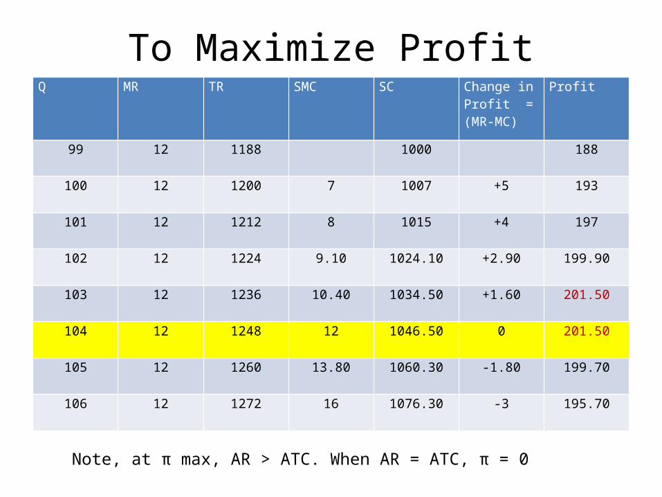
To Maximize ProfitQ MR TR SMC SC Change in

Profit = (MR-MC)

Profit

99 12 1188 1000 188

100 12 1200 7 1007 +5 193

101 12 1212 8 1015 +4 197

102 12 1224 9.10 1024.10 +2.90 199.90

103 12 1236 10.40 1034.50 +1.60 201.50

104 12 1248 12 1046.50 0 201.50

105 12 1260 13.80 1060.30 -1.80 199.70

106 12 1272 16 1076.30 -3 195.70

Note, at π max, AR > ATC. When AR = ATC, π = 0

Graphically

MR = P, SMC MC 16 13.80 12 MR = P 10.40 9.10 8 7 100 101 102 103 104 105 106 q

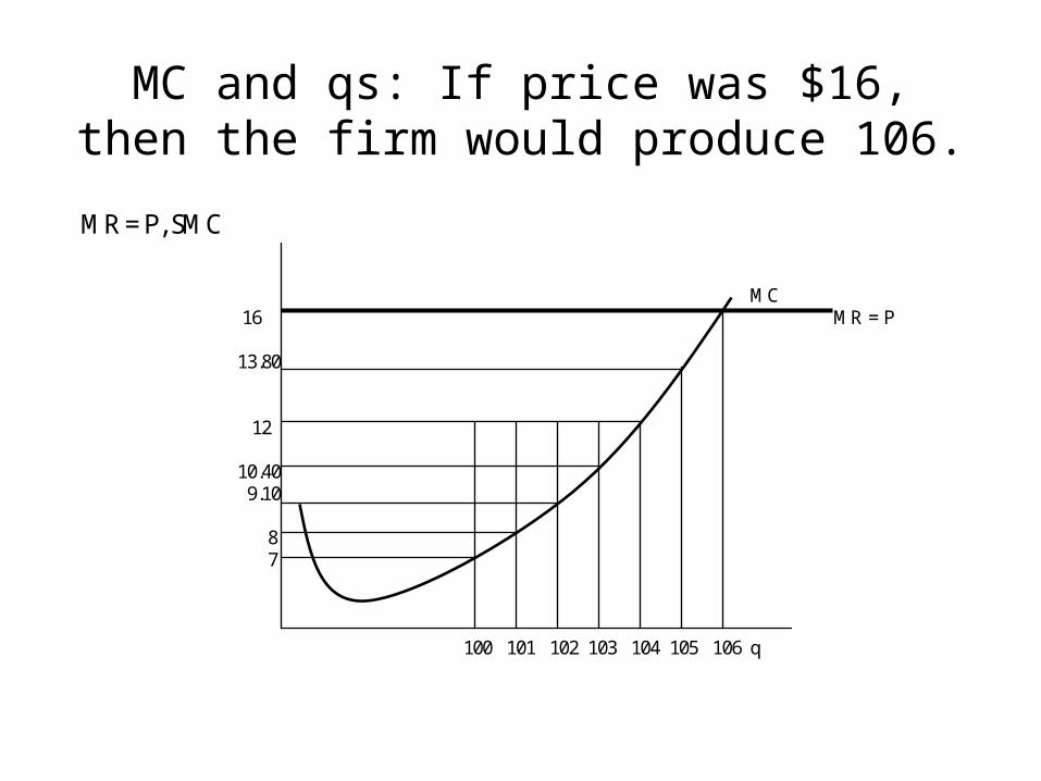
MC and qs: If price was $16, then the firm would produce 106.

MR = P, SMC MC 16 MR = P 13.80 12 10.40 9.10 8 7 100 101 102 103 104 105 106 q

MC and qs: If price was $10.40, then the firm would produce 103.

MR = P, SMC MC 16 13.80 12 MR = P 10.40 9.10 8 7 100 101 102 103 104 105 106 q

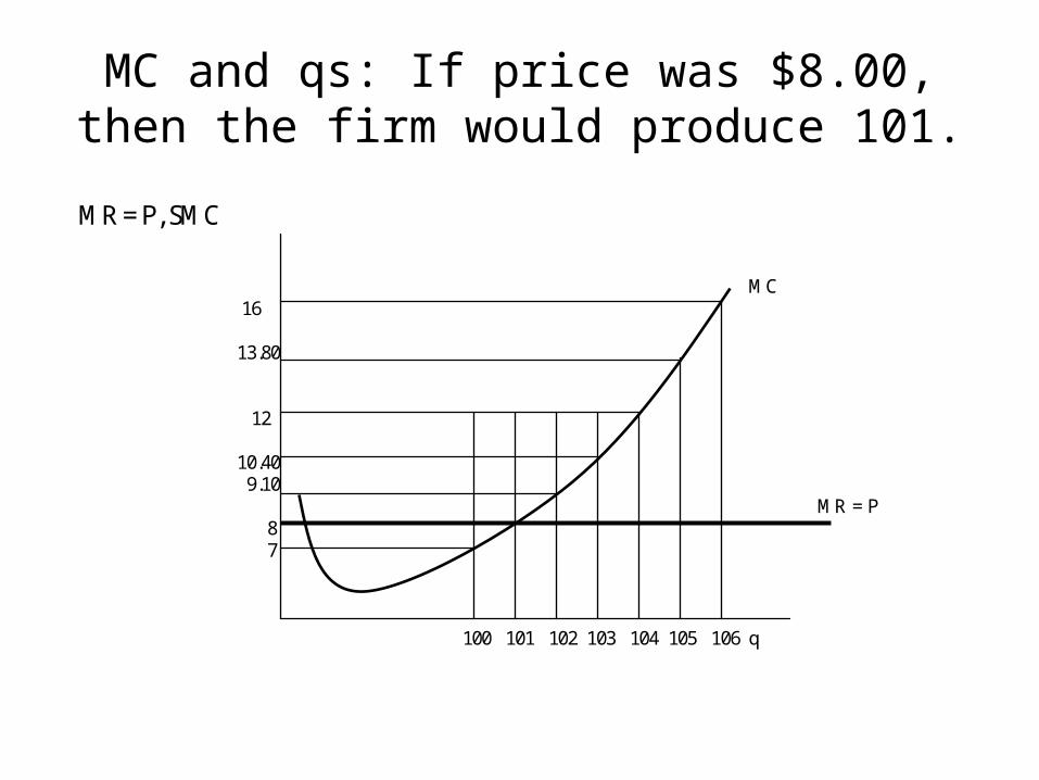
MC and qs: If price was $8.00, then the firm would produce 101.

MR = P, SMC MC 16 13.80 12 10.40 9.10 MR = P 8 7 100 101 102 103 104 105 106 q

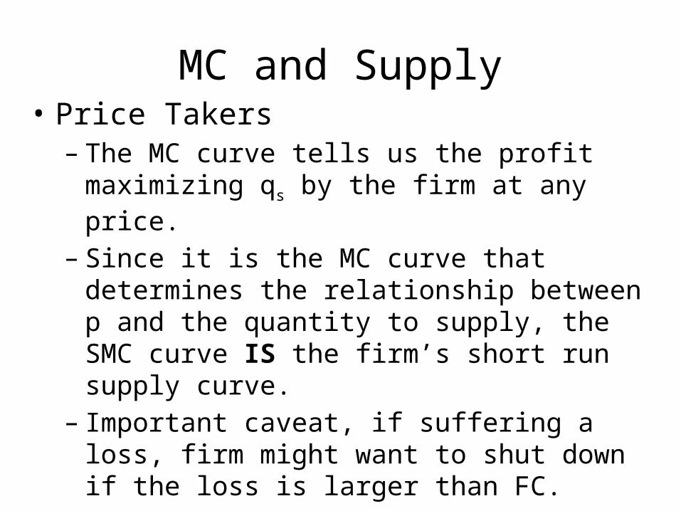
MC and Supply• Price Takers

– The MC curve tells us the profit maximizing qs by the firm at any price.

– Since it is the MC curve that determines the relationship between p and the quantity to supply, the SMC curve IS the firm’s short run supply curve.

– Important caveat, if suffering a loss, firm might want to shut down if the loss is larger than FC.

• Side note: Price Setters– set the price, they do not respond to it, so they have

no supply curve.

Shut Down Option(price takers and price setters)

• Shut down: Short run situation where the firm produces a quantity of 0 while remaining in the industry. It is still considered to be in the industry as long as it cannot rid itself from its fixed inputs.

• The firm could start producing very easily by employing some of the variable input.

Intuition• A firm bearing a loss can produce qs = q*, (where

MR=MC) or can shut down, produce qs = 0.– If qs = q*: π = R – VC – FC– If the firm shuts down: π = -FC (that is, has a loss = FC)

• If FC is greater than the loss from producing, qs = q*. If FC is less than the loss from producing qs = q*, better to shut down and produce qs=0.

• Decision Rule: Shut down if – FC > R – VC – FC

Profit from shut down

Profit from q=q*

R = 10,000VC = 8,000FC = 4,000π = -2,000

-4,000 < -2,000qs = q*

R = 7,000VC = 8,000FC = 4,000π = -5,000

-4,000 > -5,000qs =0

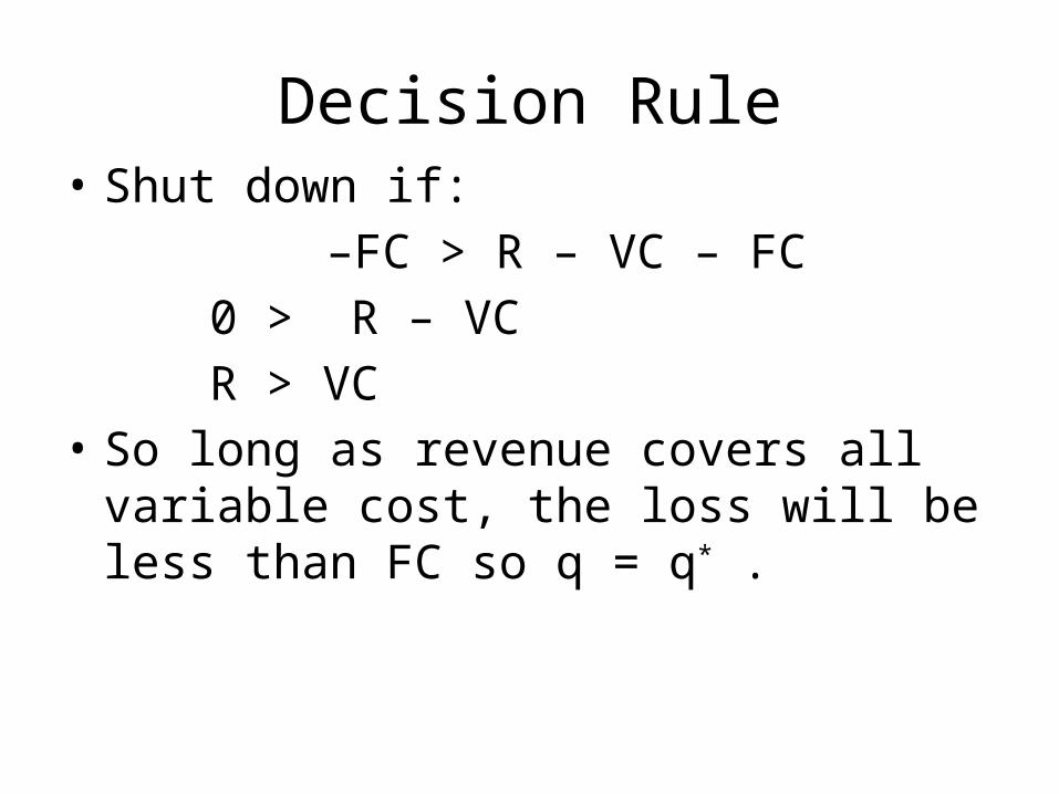
Decision Rule• Shut down if:

–FC > R – VC – FC0 > R – VCR > VC

• So long as revenue covers all variable cost, the loss will be less than FC so q = q* .

Side note: Which can change the firm’s output decision, a change in Variable Cost and/or a change in Fixed Cost?

• Shut down if: – FC > • – FC > R – VC – FC

• FC is on both sides, so a change in FC does not affect the relationship or the decision.

• Ok, yes, fixed costs are fixed (don’t vary with output)• health insurance premiums rise• Tony Romo signs a $108m extension.

• But a change in either R or VC could change the decision.

Price Taker in the Short Run

• Simple, just MR = MC• Maximize profit w.r.t. q• Maximize profit w.r.t. L

Profit Max 1

• Simple, supply is SMC, find q where SMC = p.

s

s

SC SC v,w,q;K as from last chapter SC w L w,q;K v K

dSC SMC w,q;K

dq

Set P SMC w,q;K and solve for q q p

Check to ensure that > -FC, if not, then shut down

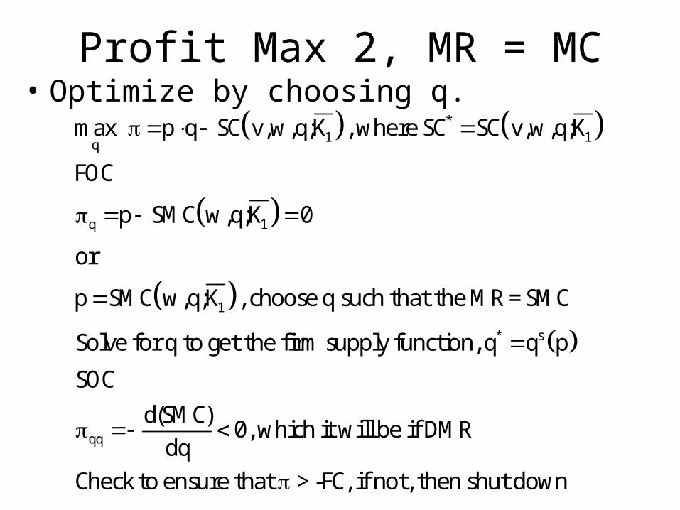
Profit Max 2, MR = MC• Optimize by choosing q.

*1 1q

q 1

1

* s

qq

max p q SC v,w,q;K , where SC SC v,w,q;K

FOC

p SMC w,q;K 0

or

p SMC w,q;K , choose q such that the MR = SMC

Solve for q to get the firm supply function, q q p

SOCd(SMC)

0, which it will be if dq

DMR

Check to ensure that > -FC, if not, then shut down

Profit Max 3, MRPL=w• Optimize by choosing L.

1 1L

L L

L L

* *1

* s1

1

max p f K ,L vK wL

FOCp f w 0

p f w, choose L such that the MRP = w

Solve for L to get the labor demand function, L L w,p,K

Plug into q f K ,L to get profit maximizing q q p

Plug into p f K ,L

1

LL LL

vK wL to get maximal profit function w,p

SOCp f 0, which it will be if DMR

Check to ensure that > -FC, if not, then shut down

Producer Surplus• Producer surplus is the amount by which a

firm is better off than shut down (q=0)• If shut down, loss is = FC• By producing, the firm covers this potential loss,

plus gains profit.• If profit = 0, then better off by the amount of FC• PS = π + FC• PS = R-VC-FC+FC• PS = R-VC

Producer Surplus

• If π = 0, then producer surplus = FC• If π < 0, but -π < FC, producer surplus > 0• If π < 0, and -π = FC, producer surplus = 0

• Shut down point• If π < 0, and -π > FC, producer surplus < 0

• Will shut down, so PS = 0 and profit = -FC.

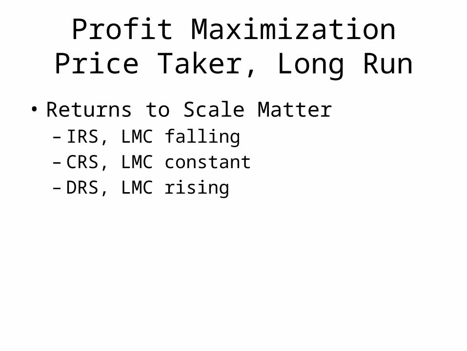
Profit MaximizationPrice Taker, Long Run

• Returns to Scale Matter– IRS, LMC falling– CRS, LMC constant– DRS, LMC rising

Increasing Returns to Scale• IRS only: incompatible with competition as the

biggest firm has the lowest average cost… natural monopoly results

C

q

ACMC

q

C

AC

MC

Decreasing Returns to Scale

• DRS only: an infinite number of infinitely small firms.

C

q

ACMC

q

C

AC

MC

Constant Returns to Scale• CRS only: any size firm can produce at the same

AC. AC = AVC = MC (Firm LRS is horizontal at MC).

C

q

ACMC

q

C

AC=MC

IRS, DRS

• IRS, DRS: MC rising. Firm LRS = MC above AC (exit otherwise.

q

ACMC

q

C

AC

ExhibitsIRS, DRS

MC

C

IRS, CRS, DRS• IRS, CRS, DRS: MC rising, but flat spot while CRS.

• Perhaps most realistic, but not easy to solve – or find a production function that creates this.

q

ACMC

q

C

AC

DRS

MC

C

IRS

CRSFirm LRS = MC for p ≥ pBE

Profit Max. vs. Perfect Comp.

ACMCSACSMC

q

ACSMC

SAC

MC

• We will eventually assume that in the long run K will be fixed to yield this SAC and the market price will be pbe (so in the LR q* will be at the low point of SAC)

• But in this chapter, we want to explore the possibility that price will exceed pbe for a while. So we need a firm LRS curve.

Firm exit if p < pBE

Production and Exit

• Essentially, a firm’s long run supply curve will be its long run MC curve…

• While shut down is a viable option in the short run, in the long run all costs can be avoided by exiting the market.

• If p < pbe, (minimum value of AC curve), the firm should exit the industry.

• So firm long run supply is MC above pbe.

Price Taker in the Long Run

• Simple, just MR = MC• Maximize profit w.r.t. q• Maximize profit w.r.t. K, L

Profit Max 1• Simple, set MC = P, find q.

* *

*

* s

C C v,w,q as from last chapter C w L v,w,q v K v,w,q

dC MC v,w,q

dq Revenue: p qdR

MR q dq

Set MR=MC and solve for q q p

d MCSOC : 0

dq Check to ensure that > -FC, if not, then shut down

Profit Max , MR=MC• Optimize by choosing q

*

q

q

*

2

qq 2

max p q C v,w,q , where C C v,w,q comes from

cost minimization.FOC

p MC v,w,q 0

or

p MC v,w,q , choose q such that the MR = MC

Solve for q to get the firm supply function, q q p

SOC

d d(MC)0

dq dq

d(MC), or 0 which it will be if DRS

dqCheck to ensure that > 0, if not, then exit

Profit Max, MRPL=w; MRPK=v• Optimize by choosing inputs

L

L L L L

K K K K

* *

*

*

* *

max p f K,L vK wL

FOCp f w 0 p f w, MRP = wp f v 0 p f v, MRP = v

Solve for L , K to get the factor demand functions

L =L(w,v,p)

K =K(w,v,p)

Plug into q f K ,L to get profit maximizing suppl

*

y function

q q K(v,w,p),L(v,w,p) q(p)

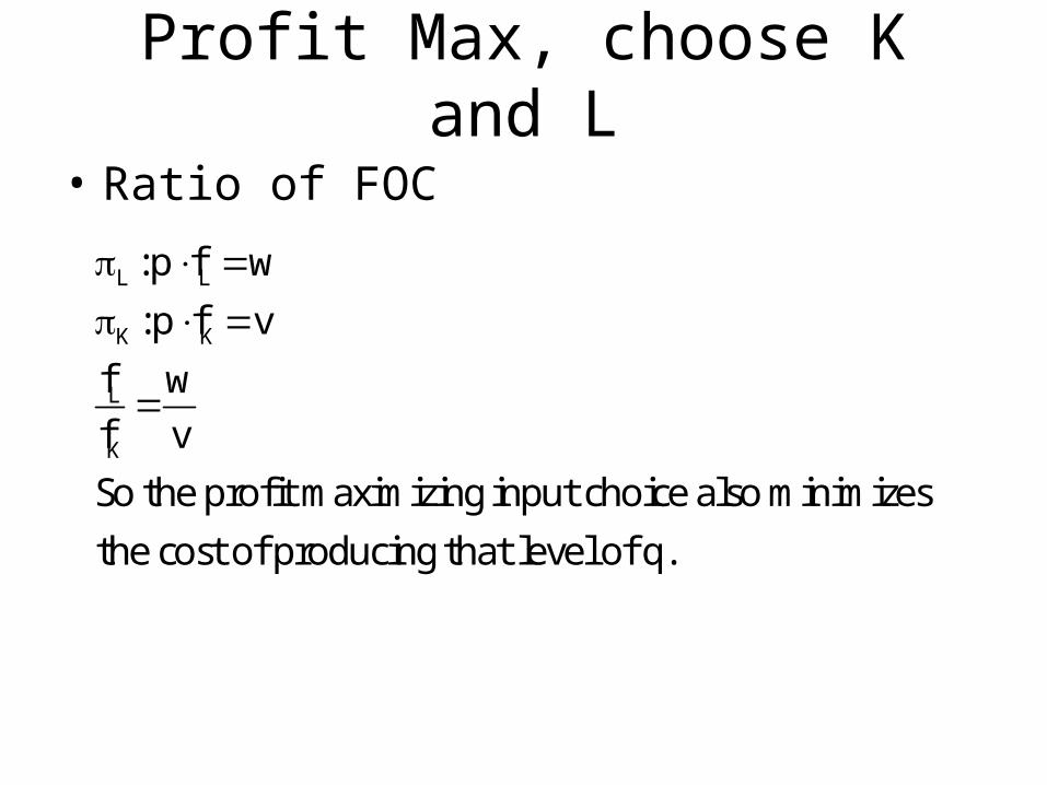
Profit Max, choose K and L

• Ratio of FOC

L L

K K

L

K

:p f w:p f v

f wf vSo the profit maximizing input choice also minimizesthe cost of producing that level of q.

Profit Max, choose K and L• SOC

* *

LL LK

KL KK

LL LL LK LK

KL KL KK KK

22LL KK LK

2LL KK LK

The function is strictly concave at L , K

H 0, negative definite

p f , p fp f , p f

H p ff f 0

So long as f 0 and f 0, and f is small.

Profit Max, choose K and L

• Profit function, maximal profits for a given w, v, and p.

* *Plug K =K(v,w,p) and L L(v,w,p) into

p f K,L vK wL

to get the profit optimizing profit function:

p f K(v,w,p),L(v,w,p) vK(v,w,p) wL(v,w,p)

Properties of the Profit Function• Homogeneous of degree one in all prices

– with inflation, K*, L*, and q* are the same profit will keep up with that inflation

• Nondecreasing in output price– Δ profit ≥ 0 with Δ p > 0

• Nonincreasing in input prices– Δ profit ≤ 0 with Δ w or Δ v > 0

• Convex in output prices– profits from averaging those from two different output prices

will be at least as large as those obtainable from the average of the two prices

1 2 1 2(p ,v,w) (p ,v,w) p p,v,w

2 2

Envelope Results• Long run supply

K p L p p p

K p L p p p

K p p L p p

p f K(v,w,p),L(v,w,p) vK(v,w,p) wL(v,w,p)

df K(v,w,p),L(v,w,p) p f K f L dp vK dp wL dp

dpd

f K(v,w,p),L(v,w,p) pf K dp pf L dp vK dp wL dpdpd

f K(v,w,p),L(v,w,p) pf K dp vK dp pf L dp wL dpdpddp

K p L p

p p

*

f K(v,w,p),L(v,w,p) pf v K dp pf w L dp

By FOCd

f K(v,w,p),L(v,w,p) 0 K dp 0 L dpdpd

f K(v,w,p),L(v,w,p) which is f(K*,L*) q*dpd

gives us the long run supply equation: q q(v,w,p)dp

df K*,L *

dp

To maximize profit when there is a change in price , q=q*= f(K*, L*), continue producing such thatL* = L(w, v, p)K* = K(w, v, p)

Envelope Results• Profit maximizing factor demand functions

*K w L w w w

*K w L w w w

*K w w L w w

*K w L w

*w w

p f K(v,w,p),L(v,w,p) vK(v,w,p) wL(v,w,p)

dp f K f L dw vK dw L wL dw

dwd

pf K dw pf L dw vK dw L wL dwdwd

pf K dw vK dw pf L dw wL dw Ldwd

pf v K dw pf w L dw LdwBy FOCd

0 K dw 0 L dw Ldw

*

By FOCd

Ldw

d gives us the demand equation, L* L(v,w,p)

dw

*

Similarly,d

K K(v,w,p)dv

To maximize profit whenthere is a change in v,K K* K(w, v, p)

To maximize profit when there is a change in w, choose L such that L = L*=L(w, v, p)

Comparative Statics

• Price taker• Long run

Comparative Statics (∂L/∂w, ∂K/∂w)

• K* and L * back into the FOC to create the following identities

L

K

* *

LL LK

* *

KL KK

p f L(w,v,p),K(w,v,p) w 0

p f L(w,v,p),K(w,v,p) v 0

differentiate w.r.t. w

L Kp f p f 1 0

w wL K

p f p f 0w w

Comparative Statics (∂L/∂w, ∂K/∂w)

*

LL LK

*KL KK

*KK

2 2LL KK LK

*KL

2 2LL KK LK

Lpf pf 1wpf pf 0K

wpfL

0w p (ff f )

pfK0

w p (ff f )

Comparative Statics(∂L/∂w, ∂K/∂w)

• Increase in wage, increases MC, q* falls

L

K

L falls, K rises

Comparative Statics(∂L/∂w, ∂K/∂w)

• Increase in wage, increases MC, q* falls

L

K

L falls, K falls

Comparative Statics (∂L/∂v, ∂K/∂v)

* *

LK KL

Note that:

L Kv w

becauseff

*

LL LK

*KL KK

*LK

2 2LL KK LK

*LL

2 2LL KK LK

Lpf pf 0vpf pf 1K

vpfL

0v p (ff f )

pfK0

v p (ff f )

Comparative Statics (∂L/∂p, ∂K/∂p)

• K* and L * back into the FOC to create the following identities

* *L

* *K

* *

L LL LK

* *

K KL KK

P f L (w,v,P),K (w,v,P) w 0

P f L (w,v,P),K (w,v,P) v 0

differentiate w.r.t. P

L Kf P f P f 0

p p

L Kf P f P f 0

p p

Comparative Statics (∂L/∂p , ∂K/∂p)

*

LL LK L

*KL KK K

*L KK K LK

2LL KK LK

*K LL L LK

2LL KK LK

Lpf pff wpf pff K

wff ffL

0p p(ff f )

ff ffK0

p p(ff f )

So long as fKL is positive or small, these will both be > 0. Since an increase in P causes MR to rise, at least one of these must be > 0

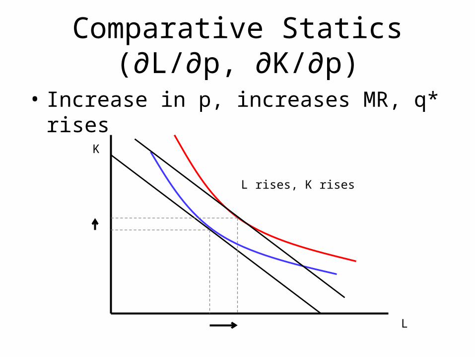
Comparative Statics(∂L/∂p, ∂K/∂p)

• Increase in p, increases MR, q* rises

L

K

L rises, K rises

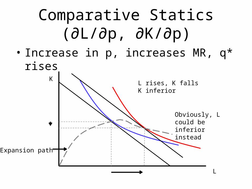
Comparative Statics(∂L/∂p, ∂K/∂p)

• Increase in p, increases MR, q* rises

L

KL rises, K fallsK inferior

Obviously, L could be inferior instead

Expansion path

Comparative Statics (∂q/∂p)• q = f(L,K)• q*=f(L*=L(w,v,p),K*=K(w,v,p))• How does this respond to a change in p?

* * *

L K

*L KK K LK

2LL KK LK

*K LL L LK

2LL KK LK

q L Kff

p p pand we now know

ff ffLp p(ff f )

ff ffKp p(ff f )

Comparative Statics (∂q/∂p)

• And so we can substitute to get:*

L KK K LK K LL L LKL K2 2

LL KK LK LL KK LK

2 2*L KK L K LK K LL

2LL KK LK

2 2L KK L K LK K LL

ff ff ff ffqff

p p(ff f ) p(ff f )and finally

ff 2ff ff fq0

p p(ff f )

where ff 2ff ff f 0 if isoquants are convex to origin(required for

2 * *LL KK LK

*

cost minimization)

where ff f 0 if production function is concave at K and L

(required for rising marginal cost at q , profit decreasing in q)

The Short Run and the Long RunLe Châteliar Principle

• How does the short run demand for L differ from the long run demand?

L

K0

K

L*

q*(w1)q*(w2)

Ls*LL

*

K2

Increase in the wage rate

Short Run Profit Max

L L

LL LL

* S

S

* SL L

max p f L,K wL vK

FOC: p f L,K w 0

SOC: p f L,K 0

Demand: L L w,p,K , once K is fixed, v does not affect L decision.

LTo get: , substitute demand (L*) into FOC

w

p f L w,p,K ,K w 0

differen

S

LL

S

LLLL

tiate w.r.t. w

Lp f 1 0

wL 1

0, as f 0w p f

Long Run vs. Short RunS

LL

LKK

2LL KK LK

L SKK

2LL KK LK LL

2L SKK LL LL KK LK

2 2LL KK LK LL LL LL KK LK

L SKK LL

L 10

w p fRemember the comparative statics result:

fL0

w p(ff f )

fL L 1w w p(ff f ) p f

ff (ff f )L Lw w p(ff f )f p f (ff f )

ffL Lw w

2 2LL KK LK LK

2 2LL KK LK LL LL LL KK LK

ff ff0

p(ff f )f pf (ff f )

> 0, by SOC

And we can deduce

Short Run Profit Max• Input demand in the long run is more elastic.

2L SLK

2LL LL KK LK

L S

L S

L S

fL L0

w w pf (ff f )

L L0

w wL L

, but both negative, so mult by -1w wL L

, LR change in L is > the short run change.w w

“These types of relations are …referred to as Le Châtelier effects, after the similar tendency of thermodynamic systems to exhibit the same types of responses.” –Silberberg, 3rd ed. (p. 85)

Cobb-Douglas Examples

• Three cases:

•

•

•

.25 .25

.5 .5

q K L

q K Lq KL

• Cost Min

.25 .25q K L

o .25 .25

.25 .25o .25 .25

L K.75 .75

minL wL vK (q L K )FOC

K LL w 0; L v 0; L q L K 0

L KwL

Expansion path: Kv

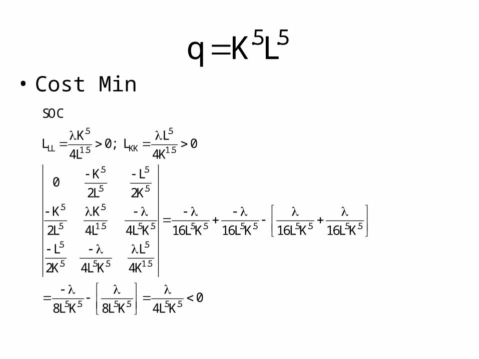
• Cost Min

.25 .25q K L

.25 .25

LL KK7 74 4

.25 .25

.75 .75

.25 .25

.75 7 .75 .75 5 5 5 5 5 5 5 54 4 4 4 4 4 4 4 4

.25 .25

.75 .75 .75 74

5 5 5 54 4 4 4

SOC

3 K 3 LL 0; L 0

4L 4K

K L0

4L 4KK 3 K 3 3

4L 4L K4L 64L K 64L K 64L K 64L KL 3 L

4K 4L K 4K

3

32L K 32L K

5 54 4

08L K

• L *, K*

• C*

.25 .25q K L

.5 .52 2

.5 .5* 2 2

.5* 2

.5 .5* *.5

.5*

v wL* q ; K* q

w v

v wC wq vq

w v

C 2q wv

pMC 4q wv ; P 4q wv ; q

4 wv

AC 2q wv

• MC, AC

.25 .25q K L

.5*

.5*

MC 4q wv

AC 2q wv

q

MC,AC

• Profit Max

.25 .25q K L

.25 .25

.25 .25

L K.75 .75

max p L K wL vK

FOC

pK pLw 0; v 0

4L 4KwL

Expansion path: Kv

• Profit Max

.25 .25q K L

.25 .25

LL KK7 74 4

.25

.25 .257 3 3 2 24 4 4

7 7.25 4 4

3 3 744 4

2

1.5

SOC

3pK 3pL0; 0

16L 16K3pK p

9p KL p KL16L 16L Kp 3pL 256 LK 256 LK

16K16L K8p

032 LK

• L *, K*

• Π*

.25 .25q K L

2 2

1.5 .5 1.5 .5

.25 .252 2*

1.5 .5 1.5 .5 .5

2 2*

.5 1.5 .5 1.5 .5

2*

.5

p pL* ; K*

16v w 16w v

p p pq

16w v 16v w 4 wv

p p pp v w

16w v 16v w4 wv

p

8 wv

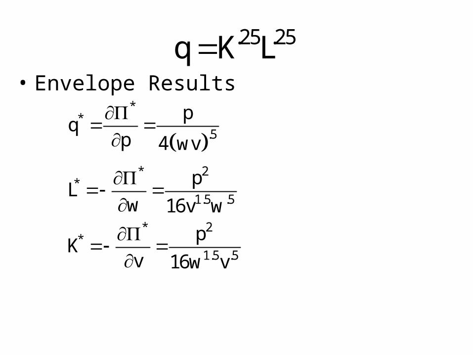
• Envelope Results

.25 .25q K L

**

.5

* 2*

1.5 .5

* 2*

1.5 .5

pq

p 4 wv

pL

w 16v wp

Kv 16w v

• Profit Max

.5*

.5*

MC 4q wv

AC 2q wv

q

MC,AC

MR

q*

2 2

1.5 .5 1.5 .5

.25 .252 2*

1.5 .5 1.5 .5 .5

p pL* ; K*

16v w 16w v

p p pq

16w v 16v w 4 wv

.25 .25q K L

• Cost Min

.5 .5q K L

o .5 .5

.5 .5o .5 .5

L K.5 .5

minL wL vK (q L K )FOC

K LL w 0; L v 0; L q L K 0

2L 2KwL

Expansion path: Kv

• Cost Min

.5 .5

LL KK1.5 1.5

.5 .5

.5 .5

.5 .5

.5 1.5 .5 .5 .5 .5 .5 .5 .5 .5 .5 .5

.5 .5

.5 .5 .5 1.5

.5 .5 .5 .5 .5 .5

SOC

K LL 0; L 0

4L 4KK L

02L 2K

K K2L 4L 4L K 16L K 16L K 16L K 16L K

L L2K 4L K 4K

08L K 8L K 4L K

.5 .5q K L

• L *, K*

• C*

.5 .5

.5 .5*

.5*

.5 .5* *

.5*

v wL* q ; K* q

w v

v wC wq vq

w v

C 2q wv

MC 4 wv ; P 4 wv ; q any

AC 2 wv

.5 .5q K L

• MC, AC

.5*

.5*

MC 2 wv

AC 2 wv

q

MC,AC

.5 .5q K L

• Profit Max

.5 .5

.5 .5

L K.5 .5

max p L K wL vK

FOC

pK pLw 0; v 0

2L 2KwL

Expansion path: Kv

.5 .5q K L

• Profit Max

.5 .5

LL KK1.5 1.5

.5

2 21.5 .5 .5

.5

.5 .5 1.5

SOC

pK pL0; 0

4L 4KpK p

p p4L 4L K 016 LK 16 LKp pL

4L K 4K

.5 .5q K L

• L *, K*

• Π*

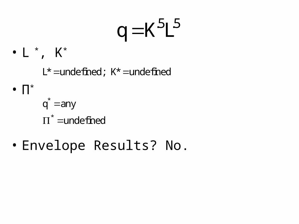
• Envelope Results? No.

*

*

L* undefined; K* undefined

q any

undefined

.5 .5q K L

• MC, AC

.5* *MC AC 2 wv

q

MC,AC

MR1

MR2

At MR1 > MC, π-max at q = ∞At MR2 < MC, π-max at q = 0At MR = MC, π-max at any q (π=0)

.5 .5q K L

• Cost Min

q KL

o

oL K

minL wL vK (q LK)FOC

L w K 0; L v L 0; L q LK 0wL

Expansion path: Kv

• Cost Min

q KL

LL KK

SOCL 0; L 0

0 K LK 0 KL KL 2KL 0L 0

• L *, K*

• C*

.5 .5

.5 .5*

.5*

.5 .5* *

2

.5*

v wL* q ; K* q

w v

v wC w q v q

w v

C 2 qwv

wv wv wvMC ; p ; q

q q p

wvAC 2

q

q KL

• MC, AC

q

MC,AC

q KL

.5*

.5*

wvAC 2

q

wvMC

q

• Profit Max

L K

max p LK wL vK

FOCpK w 0; pL v 0

wLExpansion path: K

v

q KL

Cost minimizing tangency

• Profit Max

• SOC indicate we have a profit min, not a max.

LL KK

2

SOC0; 0

0 p0 p 0

p 0

q KL

• L *, K*

• Π*

*

*

v wL* ; K*

p p

q SOC not satisfied

SOC not satisfied

q KL

• MC, AC

q

MC,AC

q KL

.5* wv

AC 2q

MR

q*

.5* wv

MCq

Maximizing profit

means q=∞, where MR ≠ MC

Only produce units where MR < MC!

AppendixShort Run vs. Long Run Labor demand

• Demand for labor can be written:

• Differentiate w.r.t. w:

• But let’s try to sign– Differentiate original equation w.r.t. v

L S LL (w,v,p) L w,p,K K (w,v,p)

S S LL L L Kw w wK

L S LL L Kv vK

The slopes of the SR and LR factor demand functions differ by a term that is the product of two effects: change in K from a change in w and the change in L that WOULD be caused by a change in the fixed amount of K.S LL K

wK

Now what?• From the differential w.r.t. v:

• Rearrange for this:

• And substitute into:

L S LL L Kv vK

sign-wise, all we know is this is < 0

Which tells us these two must have opposite signs.

L

S

L

LL v

KKv

Because of the opposite signs, this is < 0

S S LL L L Kw w wK

Now what?• Yields:

• And from reciprocity

• Yielding:

L

S L

L

LL L Kv

Kw w wv

L LL Kv w

2L

S

L

KwL LKw wv

Finally• And we can say:

• Since all terms are < 0, it is clear that the short run effect is smaller than the long run effect.

2L

S

L

KwL LKw wv

< 0

> 0