Bus Routine Profit Maximization Problem By: Shenhan Fang, Shaojie Zhang, Laura Zhang, Ran Yao

Introduction

For students at Carnegie Mellon University, the buses 61A, 61B, 61C, and 61D are most

commonly used in our everyday life not only because they all have stops at Carnegie Mellon

University, but they cover districts like Squirrel Hill, Oakland, and Downtown, where most

students live and hang out. These four types of buses are run by the Pittsburgh Port Authority.

61A and 61B cover routes from Braddock Hills Shopping Center to Downtown, 61C covers

routes from McKeesport Transportation Center to Downtown, and 61D covers routes from

Waterfront to Downtown. Usually, students take either 61A/61B, or 61C/61D because 61A and

61B go on almost the same routes and 61C and 61D have almost the same routes. For example, if

a student wants to go see a movie at Waterfront, then he/she could take either 61C or 61D to get

to the cinema directly, and if a student lives at Squirrel Hill, he/she could take either 61A or 61B

to go to school. After doing some research, we found out that the Port Authority’s operating cost

per passenger is $5.79 and each passenger pays a transfer fee of $2.75 for each ride, regardless of

the length of the ride. And after conducting surveys around CMU, we are positive to say that the

bus service provided by Pittsburgh Port Authority is very trustworthy and recognized by CMU

students, and that is why our team find it even more urgent to solve some problems that the

Pittsburgh Port Authority is facing with these buses.

Understanding the current problems

First, let us take a closer look at the schedule of these four types of bus. Each schedule

contains the inbound and outbound routes of the bus. Usually, inbound means the bus’s final

destination is Downtown Pittsburgh and outbound means the bus goes from Downtown

Pittsburgh to other districts. Each route contains around 10 stops, and it takes around 40 minutes

for 61A and 61B to finish one schedule and 50 minutes for 61C and 61D to finish one schedule.

Sample schedules of the four buses are displayed in the following page [1][2].

Current Issues

One major issue that Pittsburgh Port Authority faces is about the operating cost per

passenger and the revenue generated per passenger. Even though Port Authority is supposed to

provide fixed-time bus services, the buses are almost guaranteed to be off-schedule due to

unexpected traffic or weather conditions. The frequent off-schedule situation has caused

inconvenience to students’ daily life, resulting in a large number of students switching to Uber or

Lyft as their choice of transportation. Under this scenario, Port Authority is losing its customers

everyday and with the operating cost still remaining the same, the company is not generating as

much profit as they used to anymore.

As we proceed with this project, we decide to analyze and optimize Port Authority’s

current cost/revenue situation. Thus, our research question is: How many buses should Port

Authority dispatch on the road everyday in order to minimize operating cost and maximize

revenue generated? For the simplicity of this project, we defined some assumptions and

constraints as discussed in the “Assumptions” and “Constraints” sections.

Possible Solutions

We break our solutions down into two parts. The first part is “Base Case” and the second

part is “Simulation Method”. Within “Base Case”, we explain in detail the simplest case under

our research question. Graph, formula and real numbers are used here to demonstrate profit

generated during different time periods. Within “Simulation Method”, we simulate a much more

complex and close to reality scenario. Based on predefined assumptions and constraints, we

generate a real-time model where students are being continuously added and buses are

continuously moving forward from one station to another. With the base case served as a

foundation, we hope to use this simulation method to create a more realistic model and give

readers a better idea on how to optimize the number of buses to maximize profit for Port

Authority.

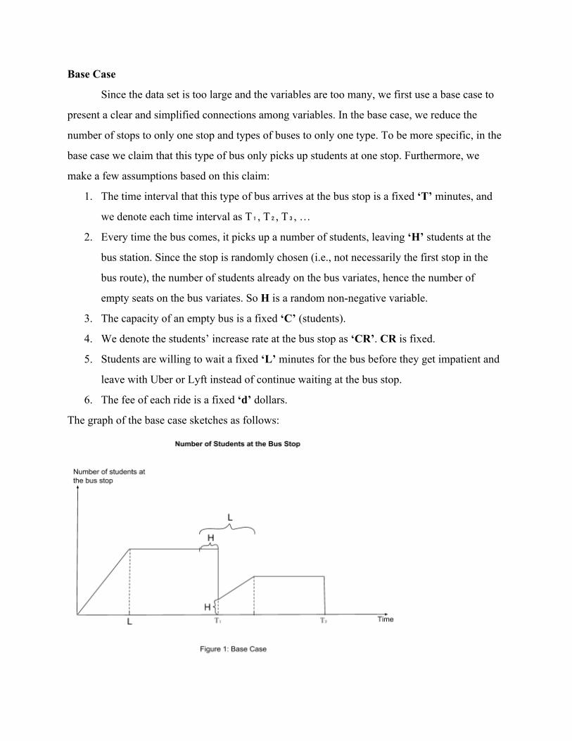
Base Case

Since the data set is too large and the variables are too many, we first use a base case to

present a clear and simplified connections among variables. In the base case, we reduce the

number of stops to only one stop and types of buses to only one type. To be more specific, in the

base case we claim that this type of bus only picks up students at one stop. Furthermore, we

make a few assumptions based on this claim:

1. The time interval that this type of bus arrives at the bus stop is a fixed ‘T’ minutes, and

we denote each time interval as T₁, T₂, T₃, …

2. Every time the bus comes, it picks up a number of students, leaving ‘H’ students at the

bus station. Since the stop is randomly chosen (i.e., not necessarily the first stop in the

bus route), the number of students already on the bus variates, hence the number of

empty seats on the bus variates. So H is a random non-negative variable.

3. The capacity of an empty bus is a fixed ‘C’ (students).

4. We denote the students’ increase rate at the bus stop as ‘CR’. CR is fixed.

5. Students are willing to wait a fixed ‘L’ minutes for the bus before they get impatient and

leave with Uber or Lyft instead of continue waiting at the bus stop.

6. The fee of each ride is a fixed ‘d’ dollars.

The graph of the base case sketches as follows:

For the sake of calculation, we assume the students’ coming rate to the bust stop is 2

students/min, student’s maximum willingness to wait is 10 minutes, the length of each time

interval is 20 minutes, bus capacity is 15 students, fee for each ride is $1.

During the first 10 minutes, the student coming rate is 2 students/min. And after 10

minutes, students start to leave with Uber, so the student coming rate and leaving rate cancel off

with each other. Hence the slope becomes 0. At the end of T₁=20 minutes, the bus comes and

picks up 15 students, leaving 10*2-15=5 students at the bus station. Therefore, the student

increase rate at the bus stop CR₂ at second interval is CR₁ from the previous period less the

student leaving rate equals . And the loop stops when H is nonpositive, R₁ ₁/(L ₁)C − H − H

meaning the students at the bus stop are all picked up by the bus.

During T₁,

₁ R apacity 0 5 studentsH = C * L − c = 2 * 1 − 1 = 5

rof it in(capacity, CR₁ ) $1 in(15, 0) 15p = m * L * = m 2 * 1 = $

During T₂,

;R₂ R₁ ₁/(L ₁) /(10 ) students/minC = C − H − H = 2 − 5 − 5 = 1

, meaning all the students can be picked₂ R₂ apacity 0 5 studentsH = C * L − c = 1 * 1 − 1 = − 5

up by the bus and there are still 5 seats empty ;

.rof it in(capacity, CR₂ ) $1 in(15, 0) 10p = m * L * = m 1 * 1 = $

Now that we have explained the base case, and before we move onto the more complicated

simulation method, the readers need to understand the assumptions and constraints that we based

our simulation model on.

Assumptions

In order to make the problem more realistic and closer to the real life situation, but at the

same time not too complicated for us to simulate, we make some assumptions to the problem.

The first such assumption is about the route. Taking into account of the fact that the buses go

through CMU like 61ABCD, we think of the bus routes of type A and B the same and the bus

route of the type C and D the same. And we also take into account that buses ABCD all share the

same routes in part of their itinerary. So our design of the route is as such: 15 stations in total,

where all of ABCD buses cover the same first 10 stations and they go separate ways after the 10th

station, where buses AB go to the same last 5 stations while CD go to the other 5 stations. And

the route is circular, meaning that after each of the buses finish their 15-station route, they will

complete their itinerary by going back to station one and then keep going. Also we make the

capacity assumption for different type of buses. Unlike in the base case where we had no

capacity roof for buses, we set the capacity of buses A and B at 40 students per bus. Similarly,

the capacity of type C and D has a 55 students limit. It is also important to note that the bus

service is only provided for students. In other words, only CMU students take these buses.

One of the most complicated assumptions we make for the problem is that the intervals

between each stations are different while the buses all travel in the same speed. To break it

down, this means that to travel from station 1 to station 2, buses ABCD will spend the same

amount of time but the travel time between stations 1 and 2 is different from that between station

2 and 3. We randomly generate the intervals between the stations by time. So it could be like that

the interval between station 1 and 2 is 3 minutes while the interval between station 3 and 4 is 6

minutes. We do realize that this is basically ignoring the speed limits and traffic, but if you think

about the Pittsburgh traffic, it really is not that bad. This assumption also entailed that the time

each bus spend at the stations can be ignored. We also assume that at the beginning, one single

bus is “generated” randomly every 10 minutes from the start station.

The next assumption we make is about the student. We assume every minute, at each

station, 3 more students show up to wait for the bus. This is probably a dialed up parameter in

the sense that on average in real life, the student coming rate at each station should be less than

3. Also, there are tricky cases where one student may have to change a bus at some point in order

to make the final destination. For example, they might get off of bus A at some point to wait for

but C. And in this case, they abandon their original student ID we assigned to the student when

they got on to bus A and they acquire a new student ID when they get on to bus C.

Constraints

The followings are the constraints given to our problem in order to do the simulation. We

try to keep in mind the fact that this problem should be solvable and that the results should make

sense as well as being economically feasible. The first constraint we introduce is that each

student has a different destination which we will pick randomly. The reason why this is a

constraint and not an assumption is that this limits the bus choice for a student. And another

constraint is that the operation cost of each bus is 300 dollars per day, including the payment for

the driver and the cost of fuel. Since we are only trying to figure out the number of buses that

will maximize our revenue, we don’t want to consider too many buses, say like 100 buses goes

around in Pittsburgh every day is just too much for this city. So we consider up to 50 buses. And

we consider a time span of 800 minutes for the purpose of our study. Last but not least, we say

that one student will wait 10 minutes for a bus before he or she run out of patience and leave the

station and take Uber or Lyft instead.

Simulation Method

To find the bus number that optimizes the total profit, we simulate the real-time situation

by continuously adding students to each bus stop, moving each bus forward to the next stop, and

removing students from the bus once they reach their destination. Here we will introduce the

general code skeleton for our simulation method. In general, we have three helper classes,

student class, bus class and stations class, in which we define the specific parameters and have

some specific methods.

1.1 Bus Class:

Each bus object has parameters busId, busType, capacity, totalStudents,

stationList, stationIdx, atStation, stationInterval dictionary and student

dictionary. The busId is uniquely assigned to each bus, and the busType can only be one out

of the all possible bus types (i.e. [A,B,C,D]). The capacity of bus is assigned corresponding to

the busType (as we stated in the assumption part). The stationList defines all the stations

ID that the bus will visit in its routine and it is ordered by the station ID. For the

stationList, each of the bus will have the same first ten common stations and then the

remaining 5 stops may differ among different type of buses. For instance, for bus1 of type A we

have bus1.stationList = [0,1,2,3,4,5,6,7,8,9,10,11,12,13,14] and for

bus2 of type B we have bus2.stationList =

[0,1,2,3,4,5,6,7,8,9,15,16,17,18,19], where the last five elements in the lists

are different. The stationIdx is the index that stationList[stationIdx] refers to the

station ID we are currently at. If the parameter atStation is true if a bus in at one station. For

instance, bus2.stationIdx = 11, bus2.stationList[11] = 15, and if

atStation = True, then bus2 is currently at station with station ID 15, otherwise bus2 is in

the process of moving from station with ID 15 to next station.And the student dictionary has key

as the student ID and value as student object.

Because it’s hard to compute the time interval between each station, we randomly

generate fixed time interval between each stops. And the stationIntervalDict has the

key as the stationed and value as the time taken to transport to next stop. As we assume all

routines are circular, then for the last stop in the stationList of each bus, the value associated with

it in the stationIntervalDict is the time to go back to initial station 0. Additionally, for

each bus object, it has method station() to return its current station (or the previous station it

just left) and method isNotFullandAtStation returns true when the bus has empty space

and is currently not in the process of moving to next station. Also, each bus has moveBus

method to move toward next station by decrementing the count in stationIntervalDict

and it also has pickUpStudents method to add new student object to its student dictionary.

1.2 Student Class:

Each student object has parameters: studentID, buses, timeArrival and

numStopsToDestination. As stated in assumption part, we assume the student ID for each

student is unique. The buses parameter defines the busType that the student can actually take in

an array. For instance, if a student can only take bus A and bus B, then the buses parameter will

be [A,B]. The numStopsToDestination defines the number of stops the student need to

stop by before they get off the bus. For instance, if numStopsToDestination = 1, then

the student will get off the bus at the next station. For each student, the most important method is

needGetOff function, which checks whether the student has reached his/her final destination.

Since it’s hard for us to collect the real-life data, we have a function

generateRandomStudent to generate student object with studentId and

timeArrival as input. And we randomly choose number between 1 and (total number of

stops - 1) as numStopstoDestination and randomly select the busType the student can

take.

1.3 Station Class:

Each station object has stationID and student dictionary as parameters. And for

each station, we have addStudent method to add a student coming to the station into the

corresponding student dictionary. Similarly, we have a removeStudent method to remove

the given student object from the student dictionary.

1.4 Main Class:

Here is pseudocode of our main function, where we iteratively to try different number of

buses using the simulation method:

Result Analysis

As stated in our research question, we want to optimize the number of buses to use every

day in order to maximize profit. Note that here profit refers to revenue generated from students

paying to get on the bus minus the fixed operating cost of the bus per day. In the following part

of this section, we present two result plots demonstrating how profit change according to the

different number of buses used. As a reminder, our simulation is based on the following main

assumptions:

(1) Total time span we study is 800 minutes

(2) Each student pay a fixed fee of $3 to get on the bus

(3) Each bus has a fixed operating cost of $300 per day

Now we look at the profit chart for profits against number of buses.

The above two plots are generated from running the simulation twice. Notice that the y-axis indicating the profit are quite different in range from the plot on the top to the one on the bottom. There are two reasons for this discrepancy in the amount of profit generated.

(1) Since the design of our model largely depends on randomly picking parameters, the results of one simulation run could be very different from another run of the simulation.

(2) Potential profit depends on the numStopToDestination parameter within the student class, i.e. how many stops a student still has until he/she reaches the final destination. In this case, when numStopToDestination is larger, this means that the bus would pick up fewer students along the way, thus leading to less profit.

(3) Potential profit also depends on the travel time interval between two adjacent stops. If the travel time interval is smaller, then buses move to the next station faster, the amount of students who switch to Uber or Lyft will be smaller, hence leading to more profit. Other than the fact that the two plots display quite different y-axis ranges, we observe

that the general trends of both plots are quite similar. Profit starts off low when only a small number of buses are used (less than 5 buses), but then profit starts to increase as we use more buses. There is a certain amount of fluctuations in the plots, but in general, we can see that the trends display an upward shift, indicating an increase in profit as we use more buses.

Looking at the two plots together, we conclude that the most amount of profit will be achieved by using 40-50 buses on the road per day.

Future Plans

Although we are able to determine the range of the number of buses to use to maximize

profit, our whole model and simulation are based on heavy assumptions, constraints and

simplification of the real-world problem. The real problem that Port Authority faces regarding

operating cost and revenue takes into account real-time traffic situations. During rush hours, the

buses are almost guaranteed to be late and that is why we often see huge amount of students

waiting for the buses between 5pm and 6pm everyday.

A more realistic and well-defined model can be included into our future research plans by

contacting Port Authority, getting real data on the amount of people who ride 61ABCD

everyday, calculating the average time that buses move from one station to another and so on…

Overall, our solution demonstrates that the Pittsburgh Port Authority bus service can

potentially be optimized to benefit both the customers and Port Authority itself. With the optimal

number of buses on the road everyday, students’ waiting time can be shortened and the

maximum profit can be ensured for Port Authority.

References

[1] Sample bus schedule for 61A and 61B. Retrieved from

http://www.portauthority.org/rt/61a.pdf

[2] Sample bus schedule for 61C and 61D. Retrieved from

http://www.portauthority.org/rt/61c.pdf