Prof. Dr.-Ing. Jochen Schiller, http://www.jochenschiller.de/

Wireless Transmission

Frequencies Signals Antenna Signal propagation

Multiplexing Spread spectrum Modulation

Frequencies for communication

VLF = Very Low Frequency UHF = Ultra High Frequency

LF = Low Frequency SHF = Super High Frequency

MF = Medium Frequency EHF = Extra High Frequency

HF = High Frequency UV = Ultraviolet Light

VHF = Very High Frequency

Frequency and wave length:

= c/f

wave length , speed of light c 3x108m/s, frequency f

1 Mm300 Hz

10 km30 kHz

100 m3 MHz

1 m300 MHz

10 mm30 GHz

100 m3 THz

1 m300 THz

visible lightVLF LF MF HF VHF UHF SHF EHF infrared UV

optical transmissioncoax cabletwisted pair

Frequencies for mobile communication

VHF-/UHF-ranges for mobile radio simple, small antenna for cars deterministic propagation characteristics, reliable connections

SHF and higher for directed radio links, satellite communication small antenna, focusing large bandwidth available

Wireless LANs use frequencies in UHF to SHF spectrum some systems planned up to EHF limitations due to absorption by water and oxygen molecules

(resonance frequencies) weather dependent fading, signal loss caused by heavy rainfall etc.

Signals I

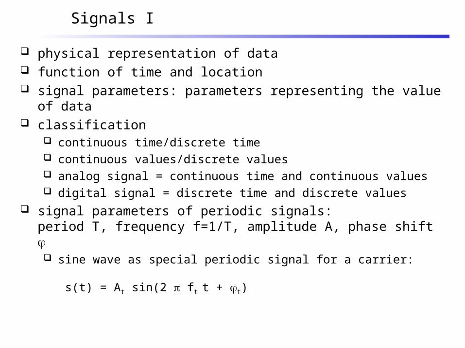
physical representation of data function of time and location signal parameters: parameters representing the value of data classification

continuous time/discrete time continuous values/discrete values analog signal = continuous time and continuous values digital signal = discrete time and discrete values

signal parameters of periodic signals: period T, frequency f=1/T, amplitude A, phase shift sine wave as special periodic signal for a carrier:

s(t) = At sin(2 ft t + t)

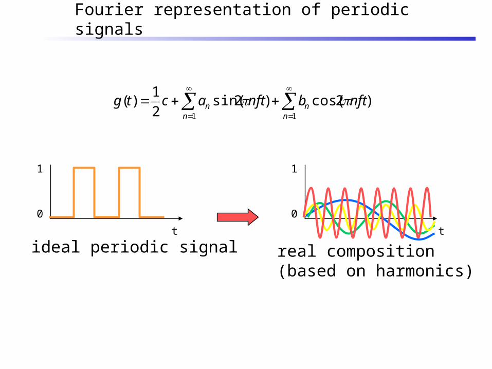
Fourier representation of periodic signals

)2cos()2sin(2

1)(

11

nftbnftactgn

nn

n

1

0

1

0

t t

ideal periodic signal real composition(based on harmonics)

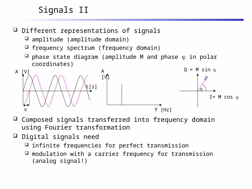
Different representations of signals amplitude (amplitude domain) frequency spectrum (frequency domain) phase state diagram (amplitude M and phase in polar coordinates)

Composed signals transferred into frequency domain using Fourier transformation

Digital signals need infinite frequencies for perfect transmission modulation with a carrier frequency for transmission (analog signal!)

Signals II

f [Hz]

A [V]

I= M cos

Q = M sin

A [V]

t[s]

Radiation and reception of electromagnetic waves, coupling of wires to space for radio transmission

Isotropic radiator: equal radiation in all directions (three dimensional) - only a theoretical reference antenna

Real antennas always have directive effects (vertically and/or horizontally)

Radiation pattern: measurement of radiation around an antenna

Antennas: isotropic radiator

zy

x

z

y x idealisotropicradiator

Antennas: simple dipoles

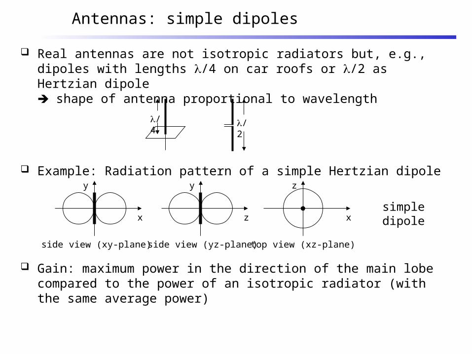
Real antennas are not isotropic radiators but, e.g., dipoles with lengths /4 on car roofs or /2 as Hertzian dipole shape of antenna proportional to wavelength

Example: Radiation pattern of a simple Hertzian dipole

Gain: maximum power in the direction of the main lobe compared to the power of an isotropic radiator (with the same average power)

side view (xy-plane)

x

y

side view (yz-plane)

z

y

top view (xz-plane)

x

z

simpledipole

/4 /2

Antennas: directed and sectorized

side view (xy-plane)

x

y

side view (yz-plane)

z

y

top view (xz-plane)

x

z

top view, 3 sector

x

z

top view, 6 sector

x

z

Often used for microwave connections or base stations for mobile phones (e.g., radio coverage of a valley)

directedantenna

sectorizedantenna

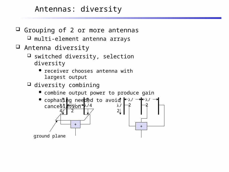
Antennas: diversity

Grouping of 2 or more antennas multi-element antenna arrays

Antenna diversity switched diversity, selection diversity

receiver chooses antenna with largest output diversity combining

combine output power to produce gain cophasing needed to avoid cancellation

+

/4/2/4

ground plane

/2/2

+

/2

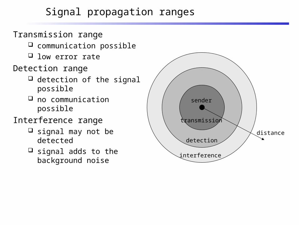
Signal propagation ranges

distance

sender

transmission

detection

interference

Transmission range communication possible low error rate

Detection range detection of the signal

possible no communication

possible

Interference range signal may not be

detected signal adds to the

background noise

Signal propagation

Propagation in free space always like light (straight line)

Receiving power proportional to 1/d² (d = distance between sender and receiver)

Receiving power additionally influenced by fading (frequency dependent) shadowing reflection at large obstacles refraction depending on the density of a medium scattering at small obstacles diffraction at edges

reflection scattering diffractionshadowing refraction

Real world example

Signal can take many different paths between sender and receiver due to reflection, scattering, diffraction

Time dispersion: signal is dispersed over time

interference with “neighbor” symbols, Inter Symbol Interference (ISI)

The signal reaches a receiver directly and phase shifted

distorted signal depending on the phases of the different parts

Multipath propagation

signal at sendersignal at receiver

LOS pulsesmultipathpulses

Effects of mobility

Channel characteristics change over time and location signal paths change different delay variations of different signal parts different phases of signal parts

quick changes in the power received (short term fading)

Additional changes in distance to sender obstacles further away

slow changes in the average power received (long term fading)

short term fading

long termfading

t

power

Multiplexing in 4 dimensions space (si)

time (t) frequency (f) code (c)

Goal: multiple use of a shared medium

Important: guard spaces needed!

s2

s3

s1

Multiplexing

f

t

c

k2 k3 k4 k5 k6k1

f

t

c

f

t

c

channels ki

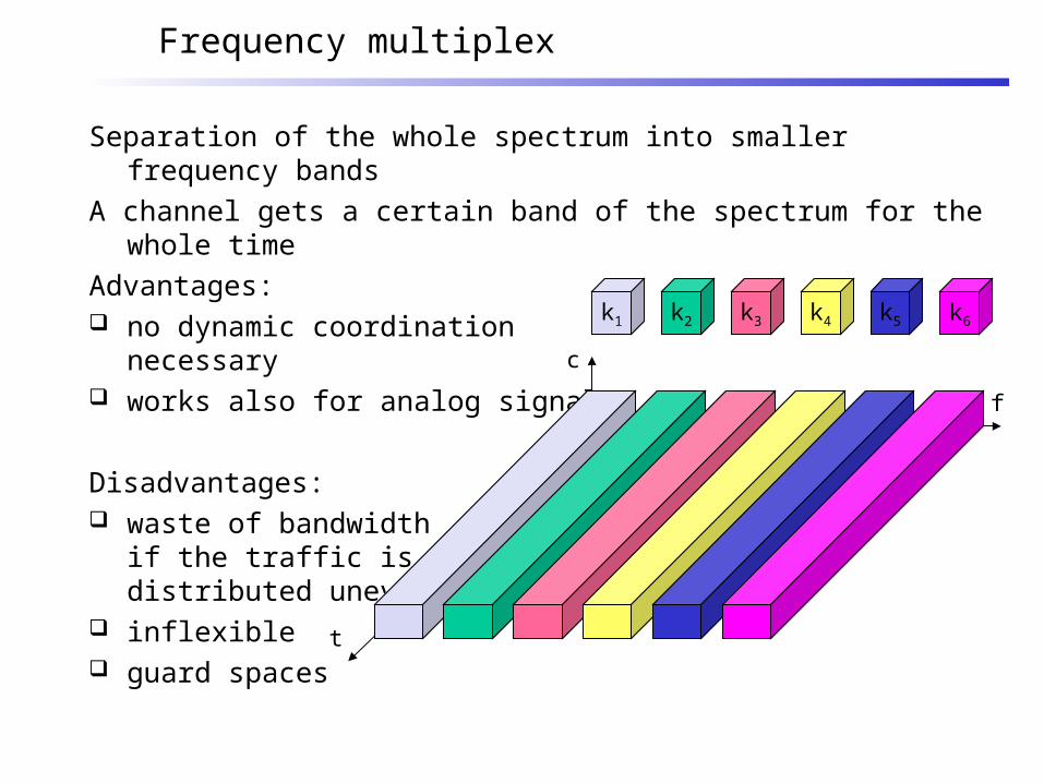
Frequency multiplex

Separation of the whole spectrum into smaller frequency bands

A channel gets a certain band of the spectrum for the whole time

Advantages: no dynamic coordination

necessary works also for analog signals

Disadvantages: waste of bandwidth

if the traffic is distributed unevenly

inflexible guard spaces

k2 k3 k4 k5 k6k1

f

t

c

f

t

c

k2 k3 k4 k5 k6k1

Time multiplex

A channel gets the whole spectrum for a certain amount of time

Advantages: only one carrier in the

medium at any time throughput high even

for many users

Disadvantages: precise

synchronization necessary

f

Time and frequency multiplex

Combination of both methods

A channel gets a certain frequency band for a certain amount of time

Example: GSM

Advantages: better protection against

tapping protection against frequency

selective interference higher data rates compared to

code multiplex

but: precise coordinationrequired

t

c

k2 k3 k4 k5 k6k1

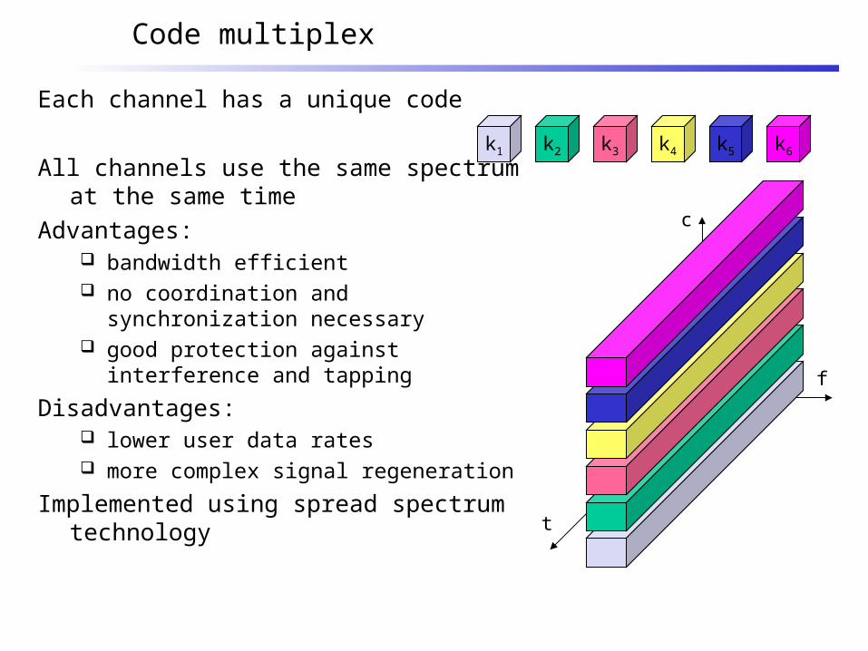
Code multiplex

Each channel has a unique code

All channels use the same spectrum at the same time

Advantages: bandwidth efficient no coordination and synchronization

necessary good protection against interference and

tapping

Disadvantages: lower user data rates more complex signal regeneration

Implemented using spread spectrum technology

k2 k3 k4 k5 k6k1

f

t

c

Modulation

Digital modulation digital data is translated into an analog signal (baseband) ASK, FSK, PSK - main focus in this chapter differences in spectral efficiency, power efficiency, robustness

Analog modulation shifts center frequency of baseband signal up to the radio carrier

Motivation smaller antennas (e.g., /4) Frequency Division Multiplexing medium characteristics

Basic schemes Amplitude Modulation (AM) Frequency Modulation (FM) Phase Modulation (PM)

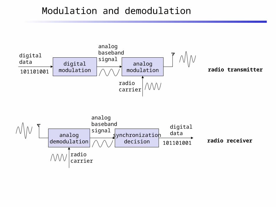
Modulation and demodulation

synchronizationdecision

digitaldataanalog

demodulation

radiocarrier

analogbasebandsignal

101101001 radio receiver

digitalmodulation

digitaldata analog

modulation

radiocarrier

analogbasebandsignal

101101001 radio transmitter

Digital modulation

Modulation of digital signals known as Shift Keying Amplitude Shift Keying (ASK):

very simple low bandwidth requirements very susceptible to interference

Frequency Shift Keying (FSK): needs larger bandwidth

Phase Shift Keying (PSK): more complex robust against interference

1 0 1

t

1 0 1

t

1 0 1

t

Advanced Frequency Shift Keying

bandwidth needed for FSK depends on the distance between the carrier frequencies

special pre-computation avoids sudden phase shifts MSK (Minimum Shift Keying)

bit separated into even and odd bits, the duration of each bit is doubled

depending on the bit values (even, odd) the higher or lower frequency, original or inverted is chosen

the frequency of one carrier is twice the frequency of the other Equivalent to offset QPSK

even higher bandwidth efficiency using a Gaussian low-pass filter GMSK (Gaussian MSK), used in GSM

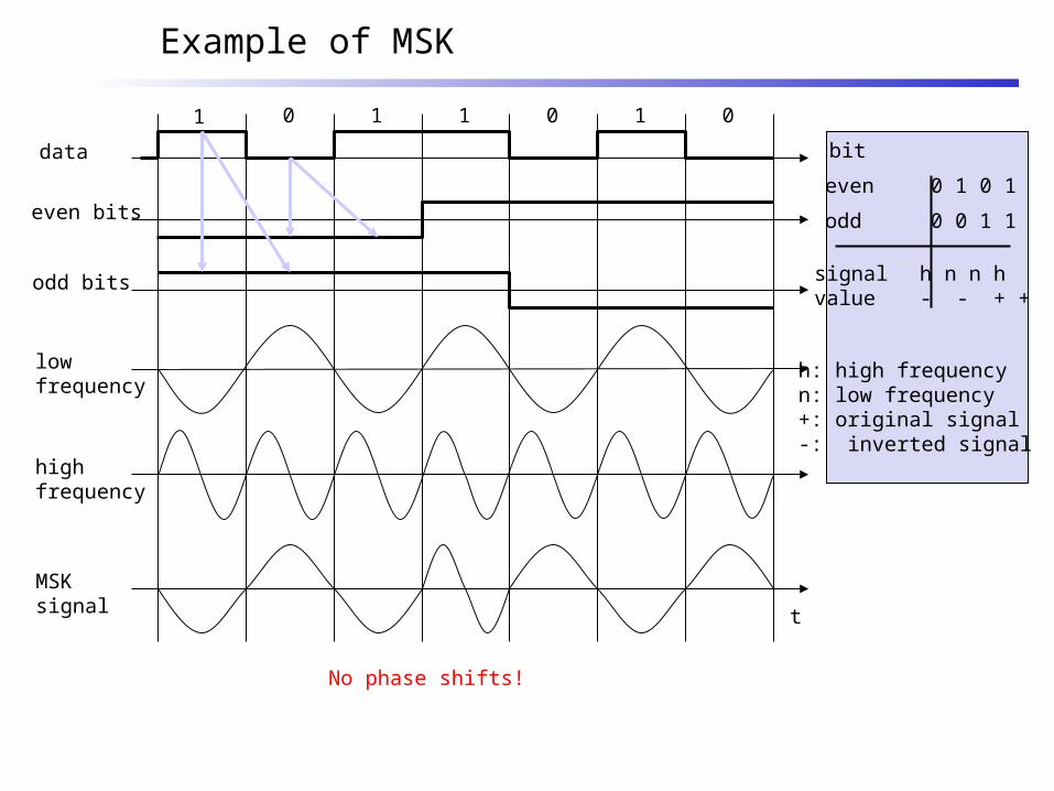
Example of MSK

data

even bits

odd bits

1 1 1 1 000

t

low frequency

highfrequency

MSKsignal

bit

even 0 1 0 1

odd 0 0 1 1

signal h n n hvalue - - + +

h: high frequencyn: low frequency+: original signal-: inverted signal

No phase shifts!

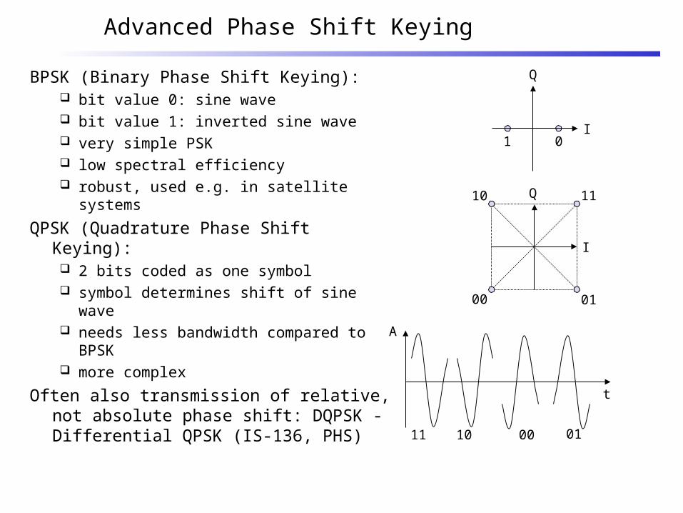
Advanced Phase Shift Keying

BPSK (Binary Phase Shift Keying): bit value 0: sine wave bit value 1: inverted sine wave very simple PSK low spectral efficiency robust, used e.g. in satellite systems

QPSK (Quadrature Phase Shift Keying): 2 bits coded as one symbol symbol determines shift of sine wave needs less bandwidth compared to

BPSK more complex

Often also transmission of relative, not absolute phase shift: DQPSK - Differential QPSK (IS-136, PHS)

11 10 00 01

Q

I01

Q

I

11

01

10

00

A

t

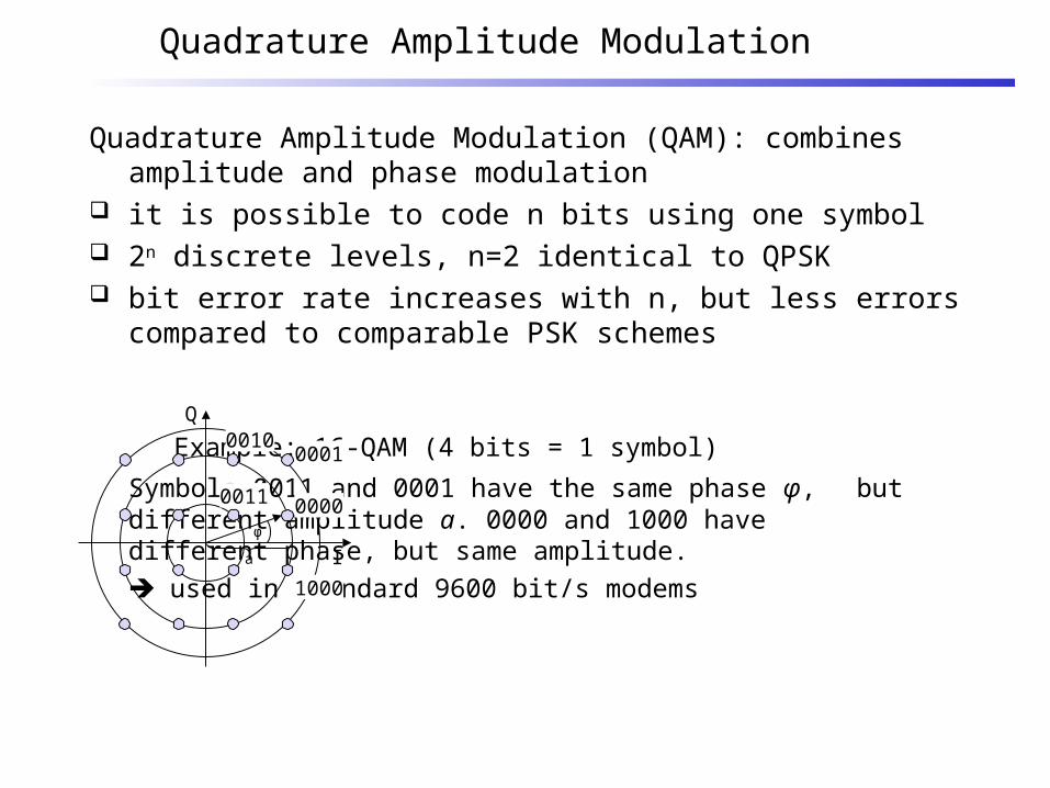
Quadrature Amplitude Modulation

Quadrature Amplitude Modulation (QAM): combines amplitude and phase modulation

it is possible to code n bits using one symbol 2n discrete levels, n=2 identical to QPSK bit error rate increases with n, but less errors compared to

comparable PSK schemes

Example: 16-QAM (4 bits = 1 symbol)

Symbols 0011 and 0001 have the same phase φ, but different amplitude a. 0000 and 1000 have different phase, but same amplitude.

used in standard 9600 bit/s modems

0000

0001

0011

1000

Q

I

0010

φ

a

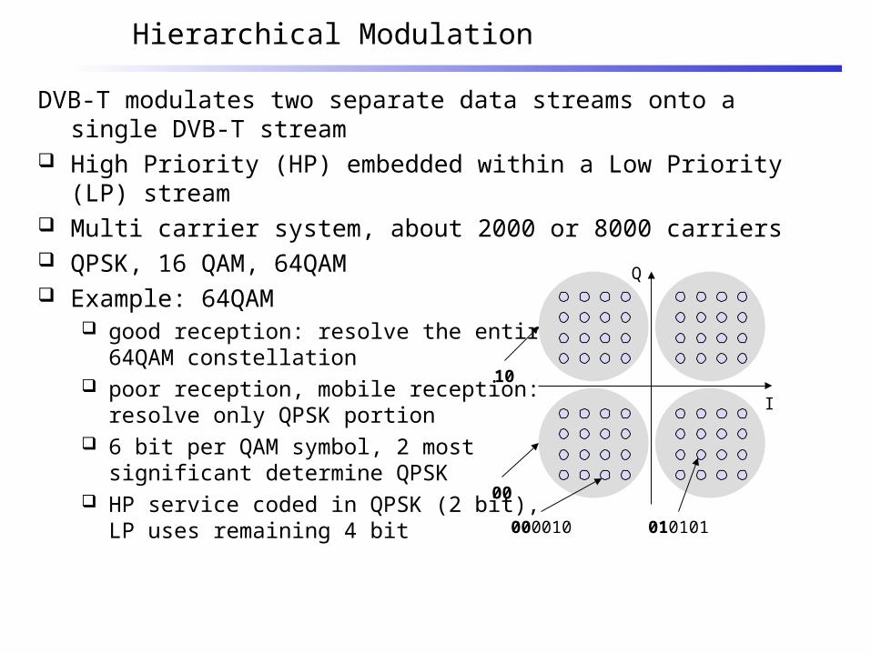
Hierarchical Modulation

DVB-T modulates two separate data streams onto a single DVB-T stream High Priority (HP) embedded within a Low Priority (LP) stream Multi carrier system, about 2000 or 8000 carriers QPSK, 16 QAM, 64QAM Example: 64QAM

good reception: resolve the entire 64QAM constellation

poor reception, mobile reception: resolve only QPSK portion

6 bit per QAM symbol, 2 most significant determine QPSK

HP service coded in QPSK (2 bit), LP uses remaining 4 bit

Q

I

00

10

000010 010101

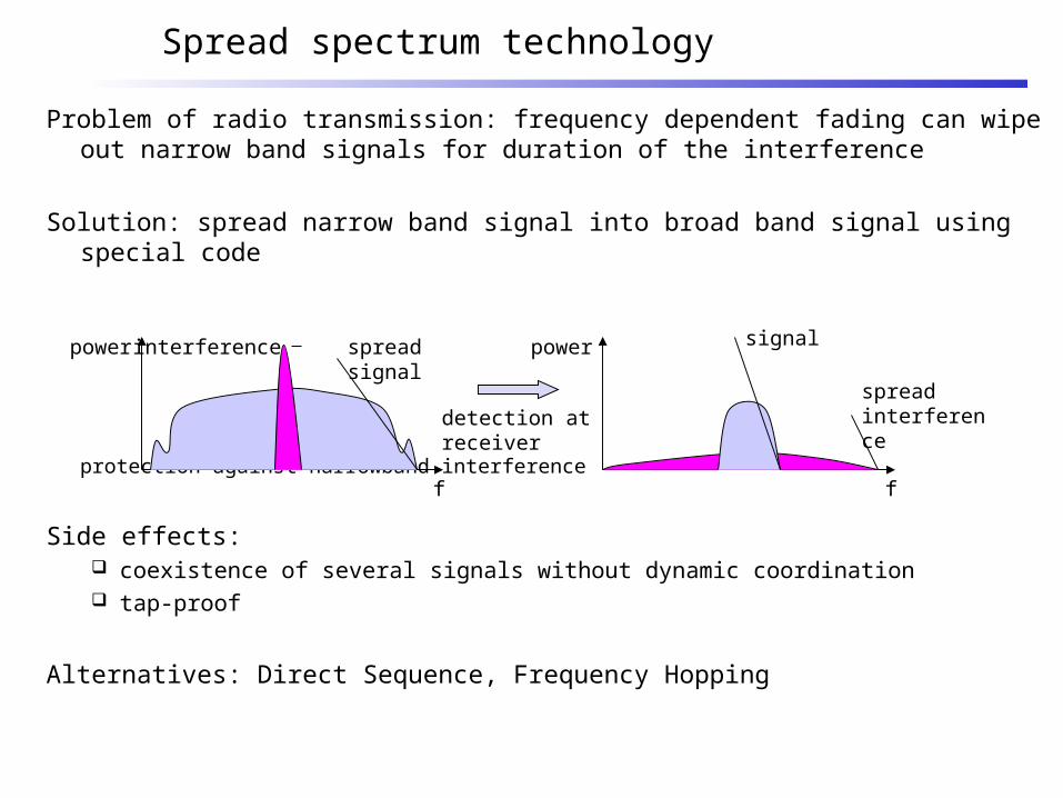
Spread spectrum technology

Problem of radio transmission: frequency dependent fading can wipe out narrow band signals for duration of the interference

Solution: spread narrow band signal into broad band signal using special code

protection against narrowband interference

Side effects: coexistence of several signals without dynamic coordination tap-proof

Alternatives: Direct Sequence, Frequency Hopping

detection atreceiver

interference spread signal

signal

spreadinterference

f f

power power

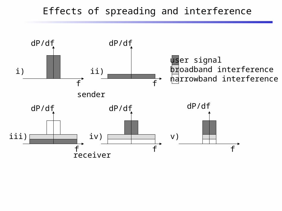
Effects of spreading and interference

dP/df

f

i)

dP/df

f

ii)

sender

dP/df

f

iii)

dP/df

f

iv)

receiverf

v)

user signalbroadband interferencenarrowband interference

dP/df

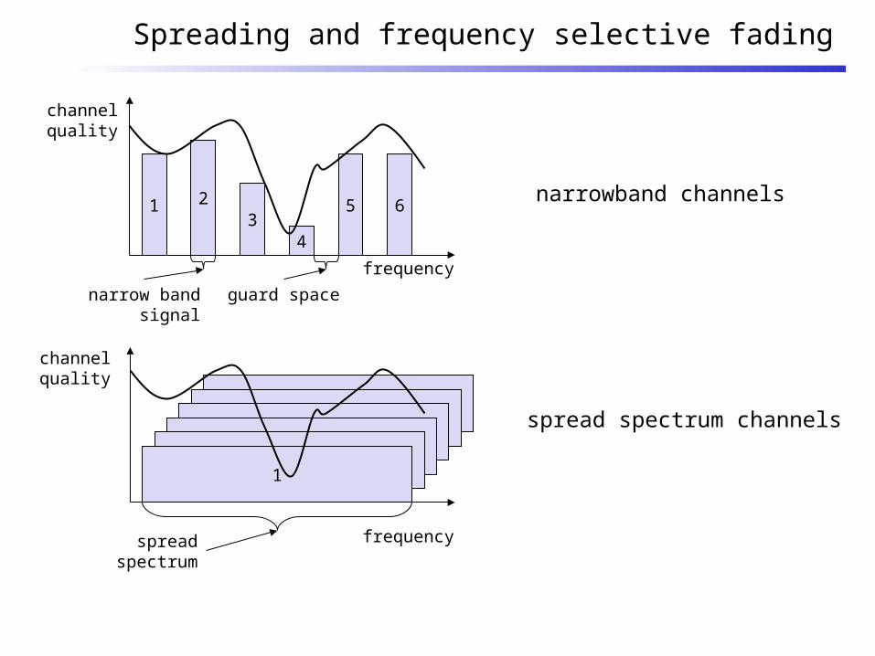
Spreading and frequency selective fading

frequency

channelquality

1 23

4

5 6

narrow bandsignal

guard space

22

22

2

frequency

channelquality

1

spreadspectrum

narrowband channels

spread spectrum channels

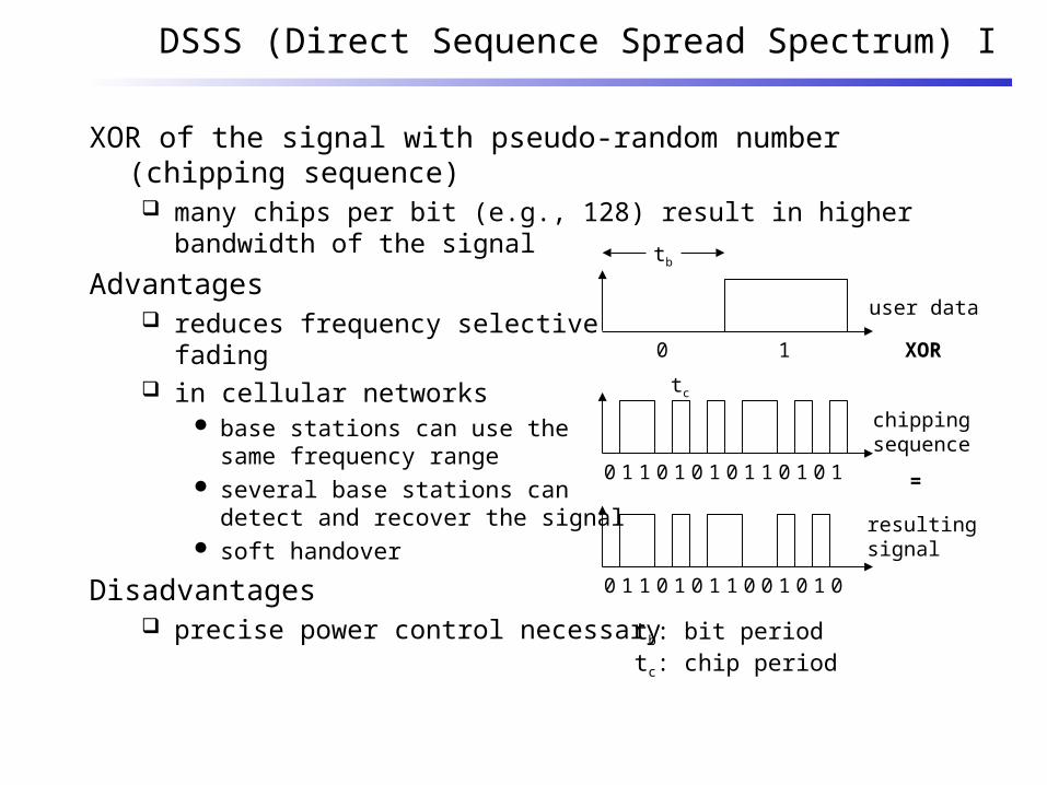
DSSS (Direct Sequence Spread Spectrum) I

XOR of the signal with pseudo-random number (chipping sequence) many chips per bit (e.g., 128) result in higher bandwidth of the signal

Advantages reduces frequency selective

fading in cellular networks

base stations can use the same frequency range

several base stations can detect and recover the signal

soft handover

Disadvantages precise power control necessary

user data

chipping sequence

resultingsignal

0 1

0 1 1 0 1 0 1 01 0 0 1 11

XOR

0 1 1 0 0 1 0 11 0 1 0 01

=

tb

tc

tb: bit periodtc: chip period

DSSS (Direct Sequence Spread Spectrum) II

Xuser data

chippingsequence

modulator

radiocarrier

spreadspectrumsignal

transmitsignal

transmitter

demodulator

receivedsignal

radiocarrier

X

chippingsequence

lowpassfilteredsignal

receiver

integrator

products

decisiondata

sampledsums

correlator

FHSS (Frequency Hopping Spread Spectrum) I

Discrete changes of carrier frequency sequence of frequency changes determined via pseudo random number

sequence

Two versions Fast Hopping:

several frequencies per user bit Slow Hopping:

several user bits per frequency

Advantages frequency selective fading and interference limited to short period simple implementation uses only small portion of spectrum at any time

Disadvantages not as robust as DSSS simpler to detect

FHSS (Frequency Hopping Spread Spectrum) II

user data

slowhopping(3 bits/hop)

fasthopping(3 hops/bit)

0 1

tb

0 1 1 t

f

f1

f2

f3

t

td

f

f1

f2

f3

t

td

tb: bit period td: dwell time

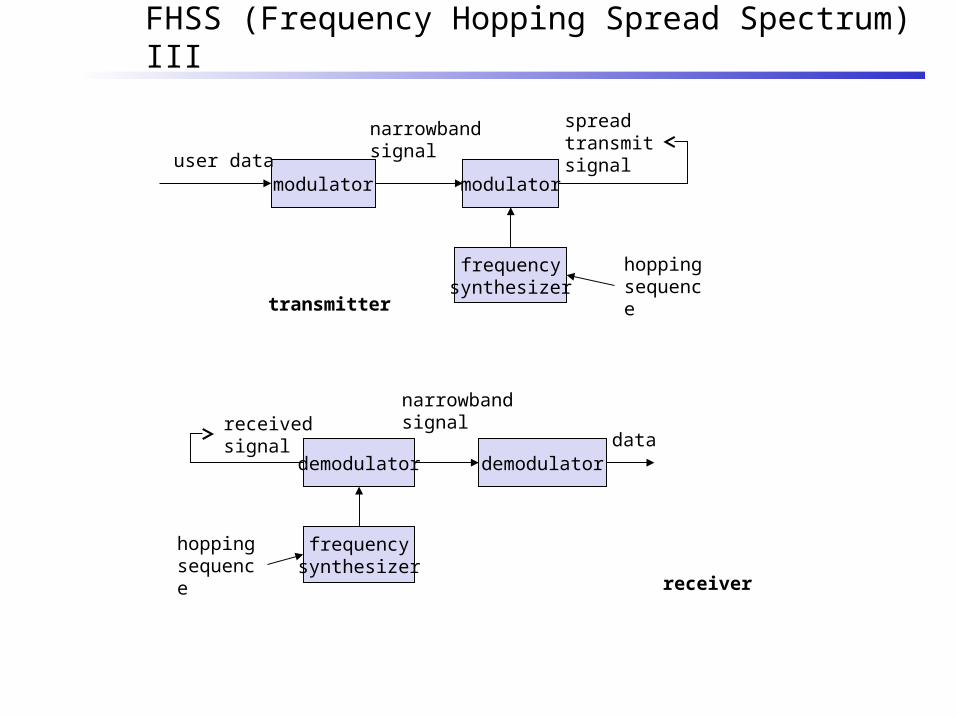
FHSS (Frequency Hopping Spread Spectrum) III

modulatoruser data

hoppingsequence

modulator

narrowbandsignal

spreadtransmitsignal

transmitter

receivedsignal

receiver

demodulatordata

frequencysynthesizer

hoppingsequence

demodulator

frequencysynthesizer

narrowbandsignal

Physical layer

Holger Karl

Receiver: Demodulation

The receiver looks at the received wave form and matches it with the data bit that caused the transmitter to generate this wave form Necessary: one-to-one mapping between data and wave form Because of channel imperfections, this is at best possible for digital

signals, but not for analog signals

Problems caused by Carrier synchronization: frequency can vary between sender and receiver

(drift, temperature changes, aging, …) Bit synchronization (actually: symbol synchronization): When does symbol

representing a certain bit start/end? Frame synchronization: When does a packet start/end? Biggest problem: Received signal is not the transmitted signal!

Attenuation results in path loss

Effect of attenuation: received signal strength is a function of the distance d between sender and transmitter

Captured by Friis free-space equation Describes signal strength at distance d relative to some reference distance

d0 < d for which strength is known

d0 is far-field distance, depends on antenna technology

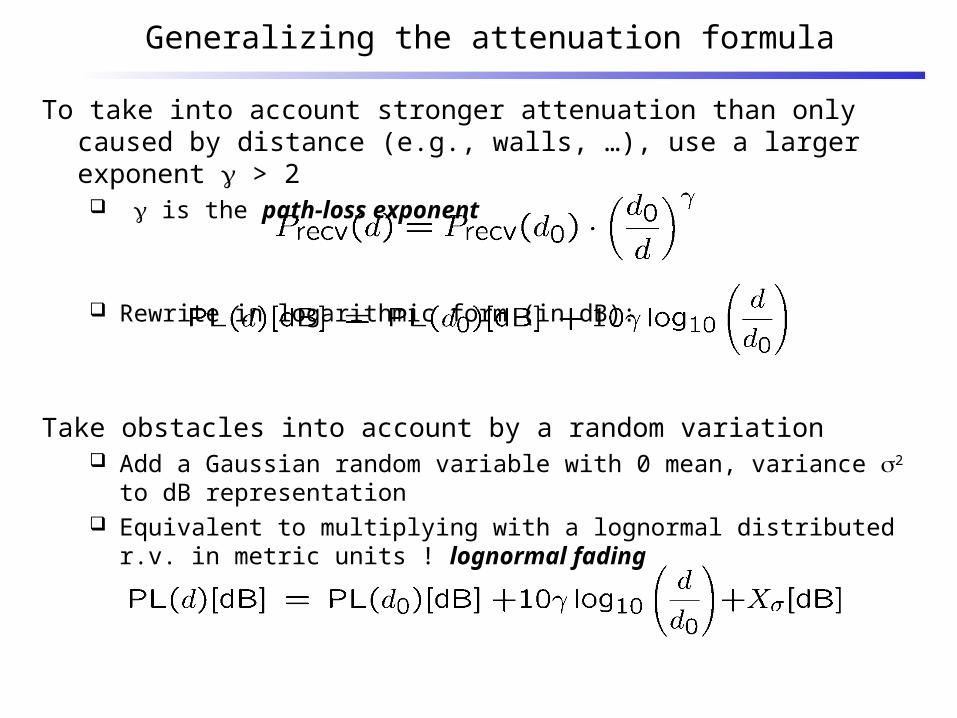
To take into account stronger attenuation than only caused by distance (e.g., walls, …), use a larger exponent > 2 is the path-loss exponent

Rewrite in logarithmic form (in dB):

Take obstacles into account by a random variation Add a Gaussian random variable with 0 mean, variance 2 to dB

representation Equivalent to multiplying with a lognormal distributed r.v. in metric units !

lognormal fading

Generalizing the attenuation formula

Noise and interference

So far: only a single transmitter assumed Only disturbance: self-interference of a signal with multi-path “copies” of

itself

In reality, two further disturbances Noise – due to effects in receiver electronics, depends on temperature

Typical model: an additive Gaussian variable, mean 0, no correlation in time Interference from third parties

Co-channel interference: another sender uses the same spectrum Adjacent-channel interference: another sender uses some other part of the

radio spectrum, but receiver filters are not good enough to fully suppress it

Effect: Received signal is distorted by channel, corrupted by noise and interference What is the result on the received bits?

Symbols and bit errors

Extracting symbols out of a distorted/corrupted wave form is fraught with errors Depends essentially on strength of the received signal compared to the

corruption Captured by signal to noise and interference ratio (SINR)

SINR allows to compute bit error rate (BER) for a given modulation Also depends on data rate (# bits/symbol) of modulation E.g., for simple DPSK, data rate corresponding to bandwidth:

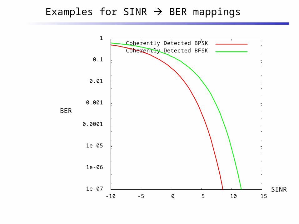
Examples for SINR BER mappings

1e-07

1e-06

1e-05

0.0001

0.001

0.01

0.1

1

-10 -5 0 5 10 15

Coherently Detected BPSKCoherently Detected BFSK

BER

SINR

Channel models – analog

How to stochastically capture the behavior of a wireless channel Main options: model the SNR or directly the bit errors

Signal models Simplest model: assume transmission power and attenuation are constant,

noise an uncorrelated Gaussian variable Additive White Gaussian Noise model, results in constant SNR

Situation with no line-of-sight path, but many indirect paths: Amplitude of resulting signal has a Rayleigh distribution (Rayleigh fading)

One dominant line-of-sight plus many indirect paths: Signal has a Rice distribution (Rice fading)

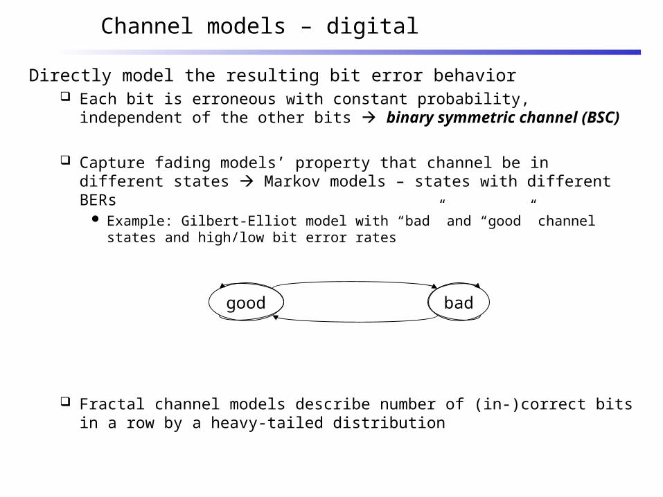
Channel models – digital

Directly model the resulting bit error behavior Each bit is erroneous with constant probability, independent of the other

bits binary symmetric channel (BSC)

Capture fading models’ property that channel be in different states Markov models – states with different BERs

Example: Gilbert-Elliot model with “bad” and “good” channel states and high/low bit error rates

Fractal channel models describe number of (in-)correct bits in a row by a heavy-tailed distribution

good bad

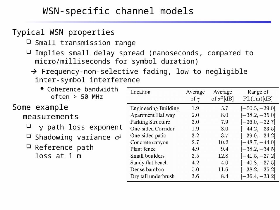
WSN-specific channel models

Typical WSN properties Small transmission range Implies small delay spread (nanoseconds, compared to micro/milliseconds

for symbol duration)

Frequency-non-selective fading, low to negligible inter-symbol interference Coherence bandwidth

often > 50 MHz

Some example measurements path loss exponent Shadowing variance 2 Reference path

loss at 1 m

Wireless channel quality – summary

Wireless channels are substantially worse than wired channels In throughput, bit error characteristics, energy consumption, …

Wireless channels are extremely diverse There is no such thing as THE typical wireless channel

Various schemes for quality improvement exist Some of them geared towards high-performance wireless communication –

not necessarily suitable for WSN, ok for MANET Diversity, equalization, …

Some of them general-purpose (ARQ, FEC) Energy issues need to be taken into account!

Some transceiver design considerations

Strive for good power efficiency at low transmission power Some amplifiers are optimized for efficiency at high output power To radiate 1 mW, typical designs need 30-100 mW to operate the

transmitter WSN nodes: 20 mW (mica motes)

Receiver can use as much or more power as transmitter at these power levels

! Sleep state is important

Startup energy/time penalty can be high Examples take 0.5 ms and ¼ 60 mW to wake up

Exploit communication/computation tradeoffs Might payoff to invest in rather complicated coding/compression schemes

Choice of modulation

One exemplary design point: which modulation to use? Consider: required data rate, available symbol rate, implementation

complexity, required BER, channel characteristics, … Tradeoffs: the faster one sends, the longer one can sleep

Power consumption can depend on modulation scheme Tradeoffs: symbol rate (high?) versus data rate (low)

Use m-ary transmission to get a transmission over with ASAP But: startup costs can easily void any time saving effects For details: see example in exercise!

Adapt modulation choice to operation conditions Akin to dynamic voltage scaling, introduce Dynamic Modulation Scaling

Summary

Wireless radio communication introduces many uncertainties and vagaries into a communication system

Handling the unavoidable errors will be a major challenge for the communication protocols

Dealing with limited bandwidth in an energy-efficient manner is the main challenge

MANET and WSN are pretty similar here Main differences are in required data rates and resulting transceiver

complexities (higher bandwidth, spread spectrum techniques)

Wireless Communications

Principles and Practice2nd EditionT.S. Rappaport

Chapter 4: Mobile Radio Propagation: Large-Scale Path Loss

Co-channel and Adjacent Channel Interference, Propagation

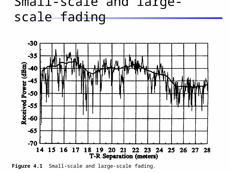
Small-scale and large-scale fading

Figure 4.1 Small-scale and large-scale fading.

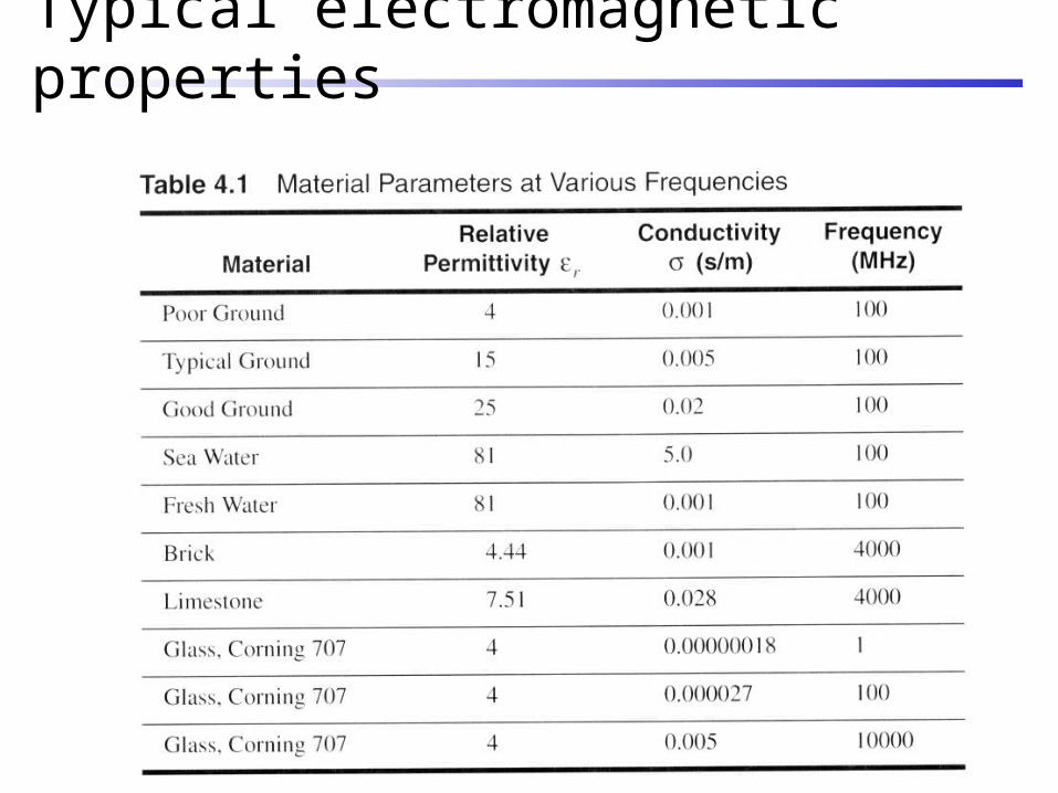
Typical electromagnetic properties

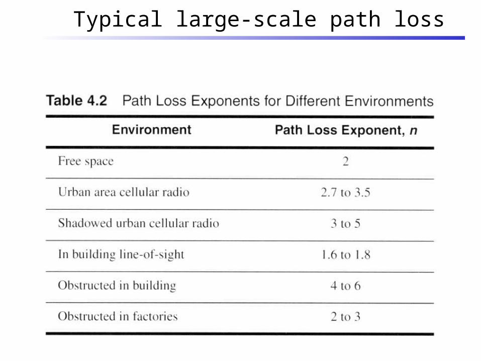
Typical large-scale path loss

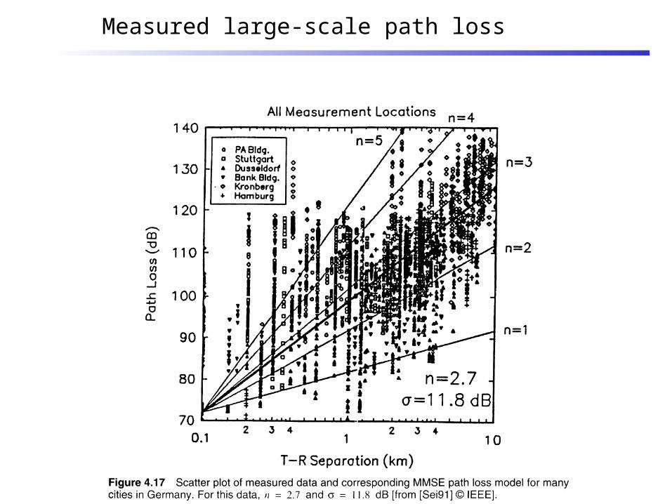
Measured large-scale path loss

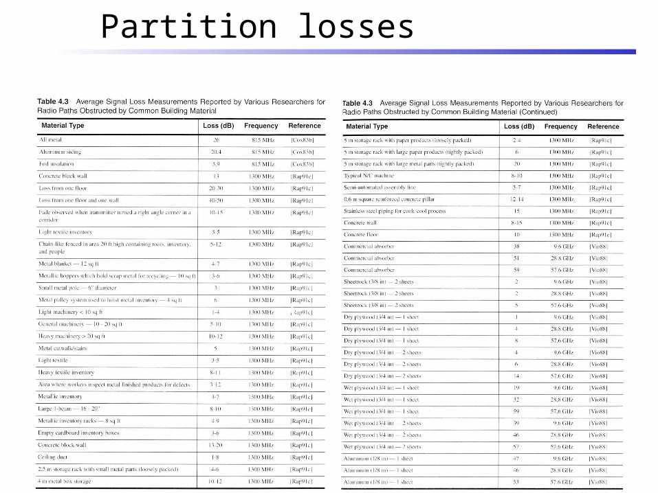
Partition losses

Partition losses

Partition losses

Wireless Communications

Principles and Practice2nd EditionT.S. Rappaport

Chapter 5: Mobile Radio Propagation: Small-Scale Fading and Multipath as it applies to Modulation Techniques

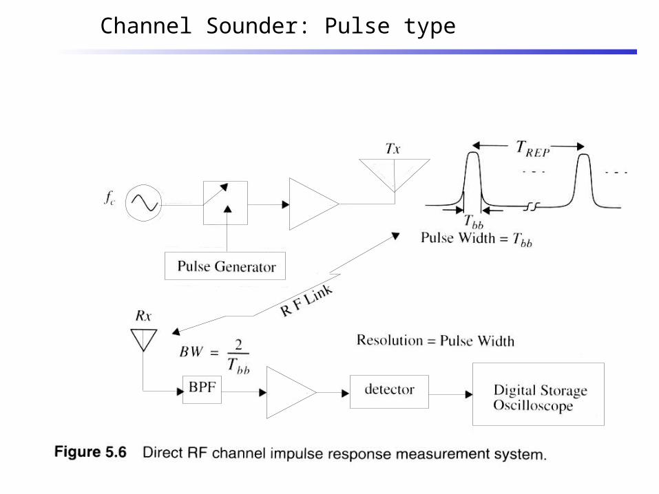
Channel Sounder: Pulse type

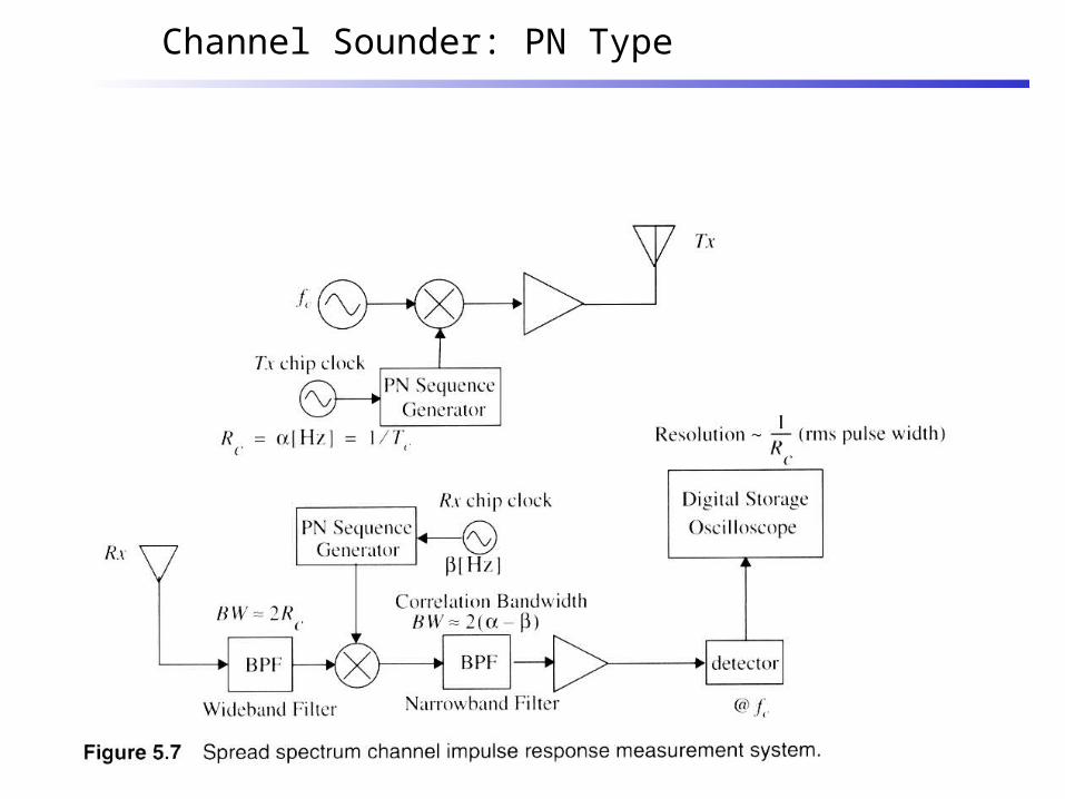
Channel Sounder: PN Type

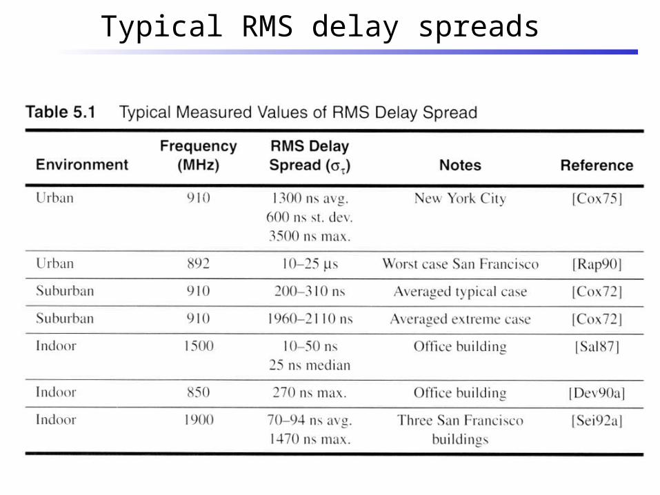
Typical RMS delay spreads

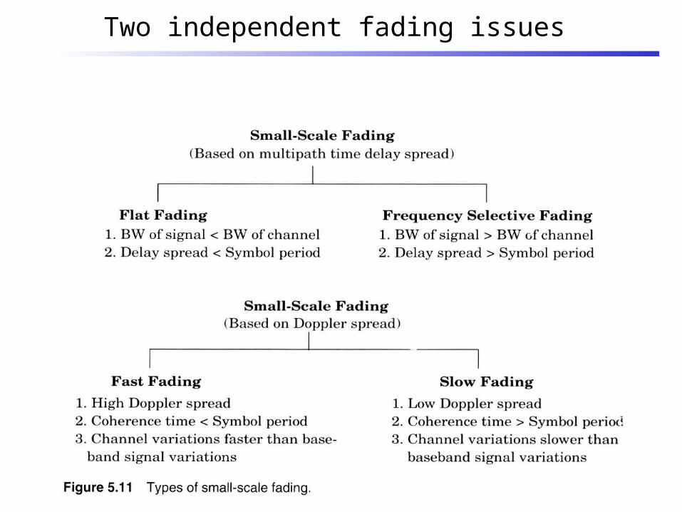
Two independent fading issues

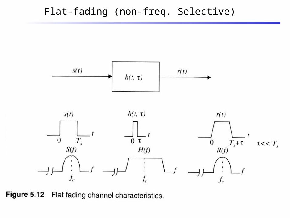
Flat-fading (non-freq. Selective)

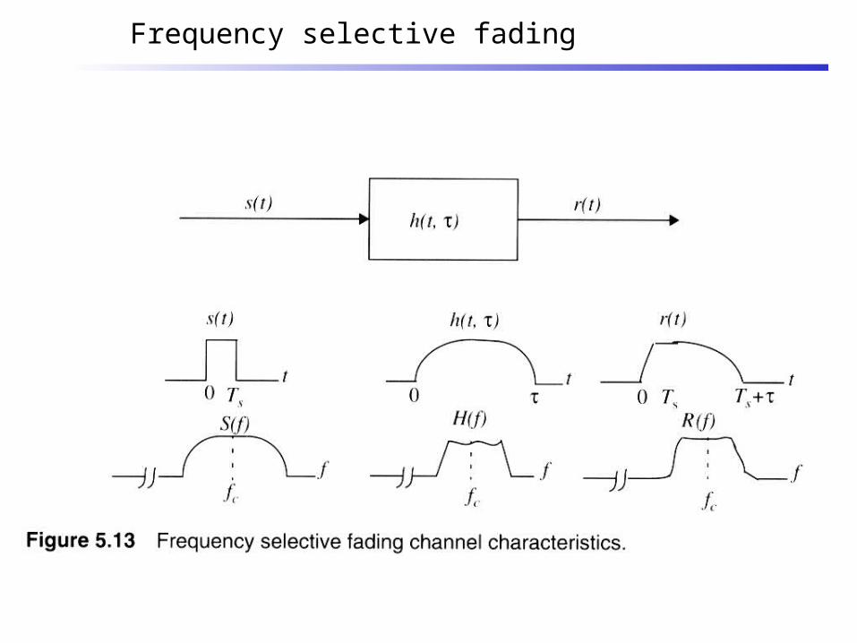
Frequency selective fading

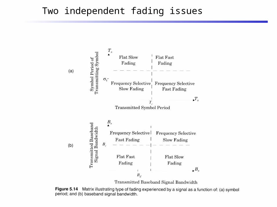
Two independent fading issues

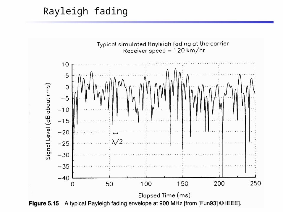
Rayleigh fading

Small-scale envelope distributions

Ricean and Rayleigh fading distributions

Wireless Communications

Principles and Practice2/eT.S. Rapppaport

Chapter 6: Modulation Techniques for Mobile Radio

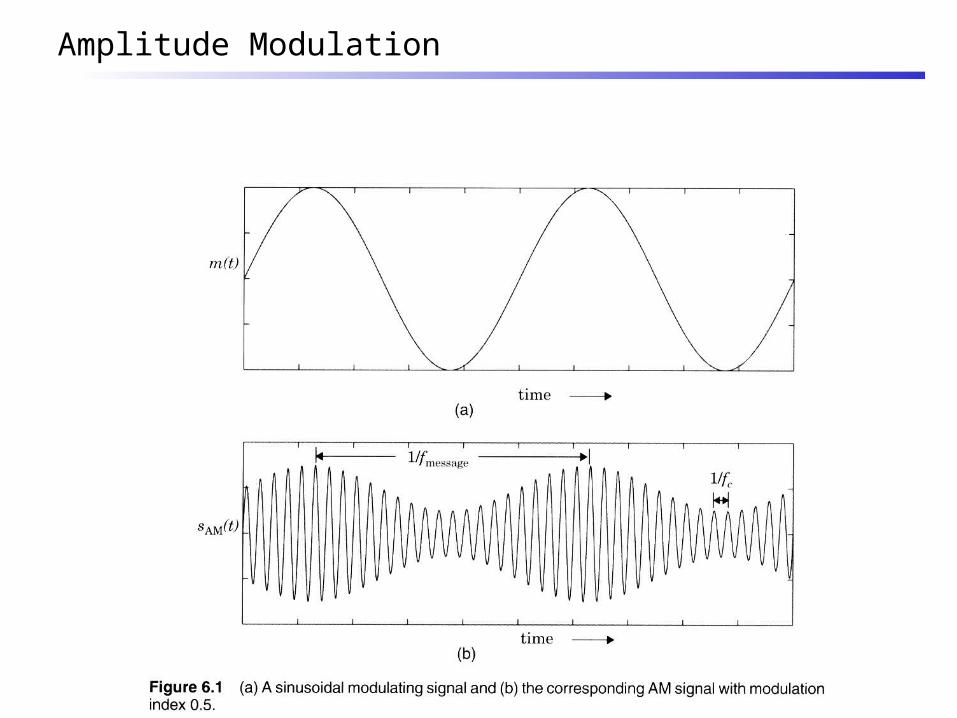
Amplitude Modulation

Double Sideband Spectrum

SSB Modulators

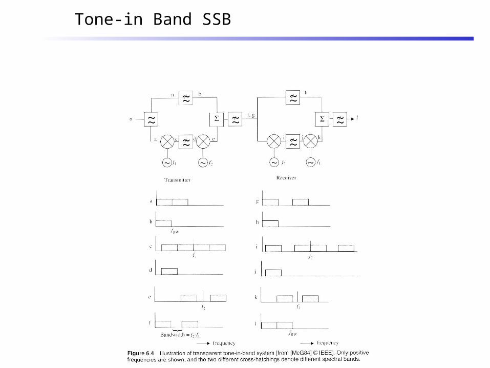
Tone-in Band SSB

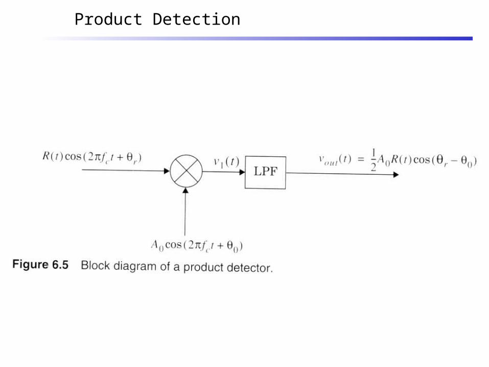
Product Detection

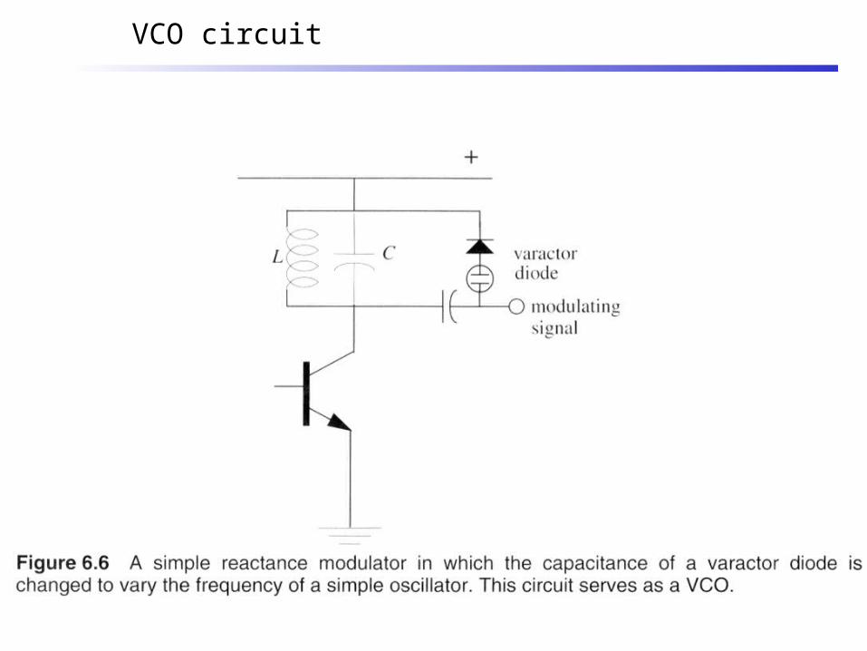
VCO circuit

Wideband FM generation

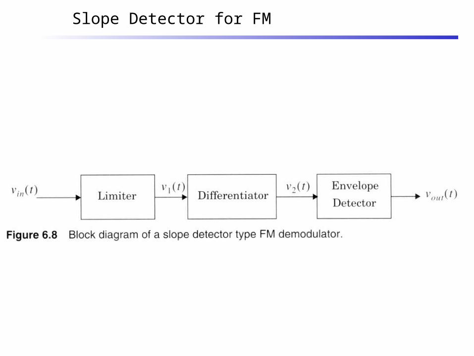
Slope Detector for FM

Digital Demod for FM

PLL Demod for FM

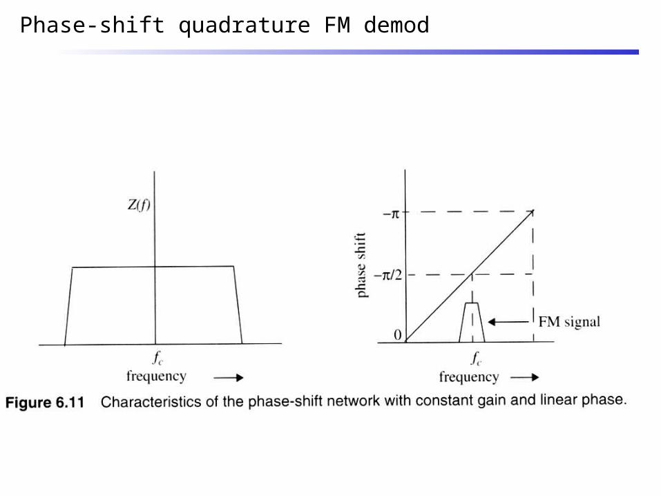
Phase-shift quadrature FM demod

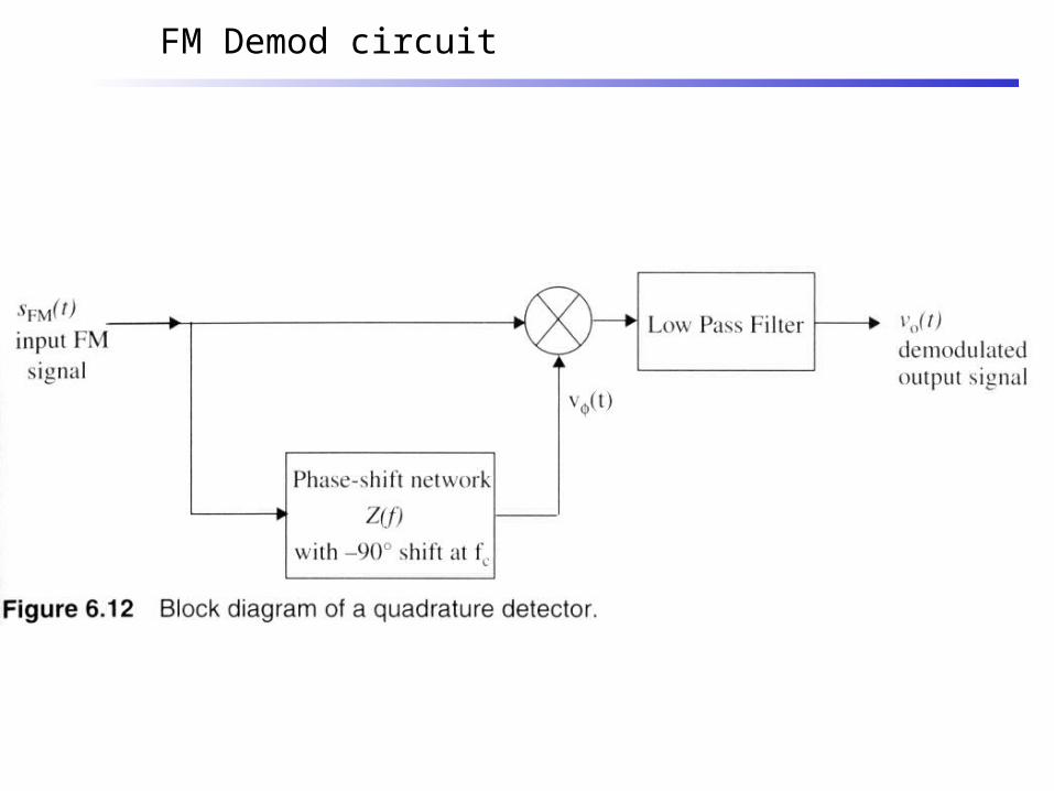
FM Demod circuit

Line Coding spectra

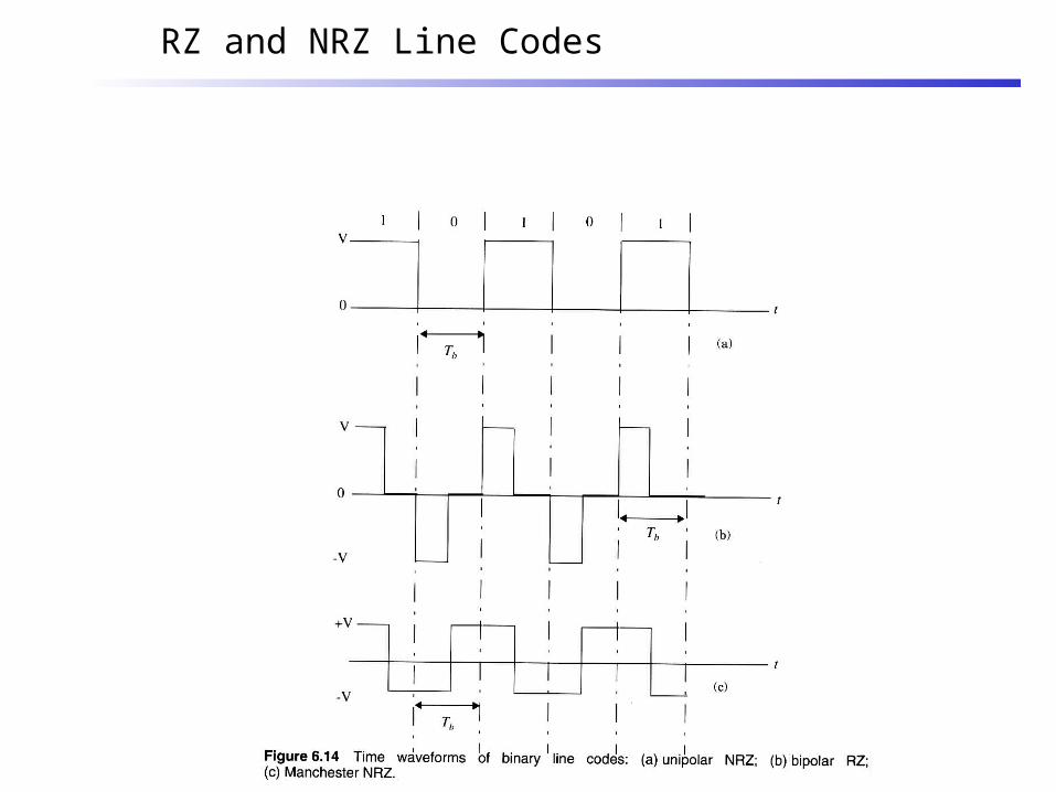
RZ and NRZ Line Codes

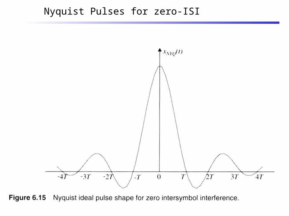
Nyquist Pulses for zero-ISI

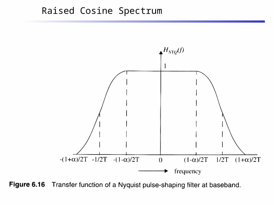
Raised Cosine Spectrum

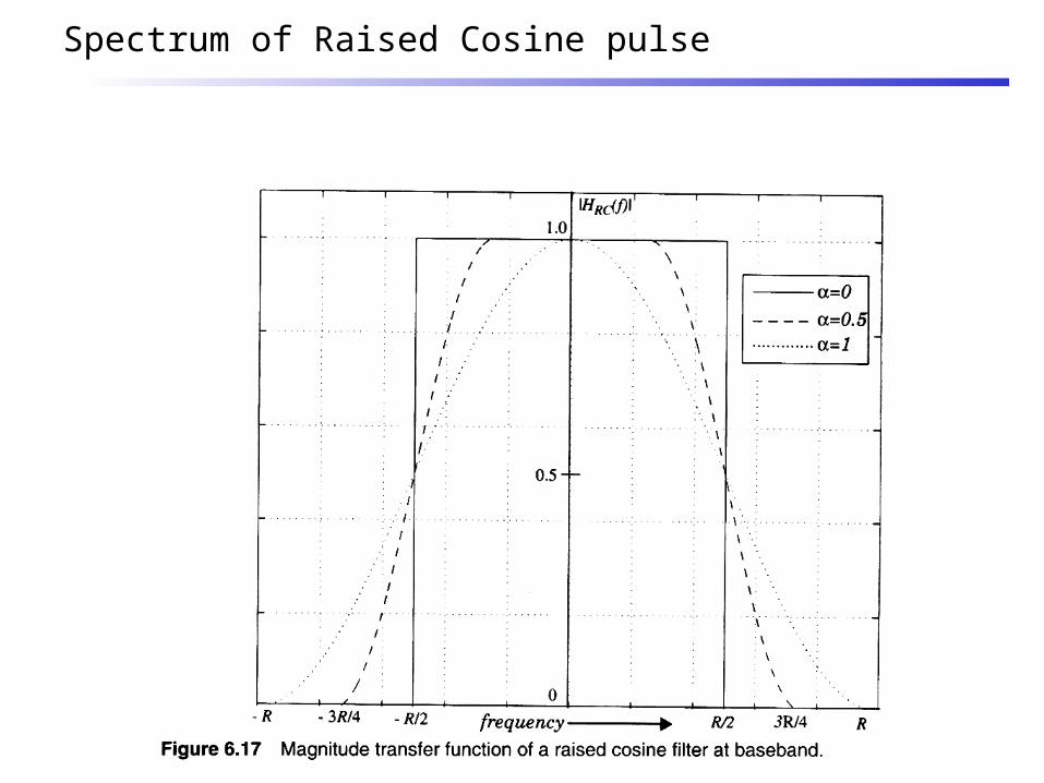
Spectrum of Raised Cosine pulse

Raised Cosine pulses

RF signal usig Raised Cosine

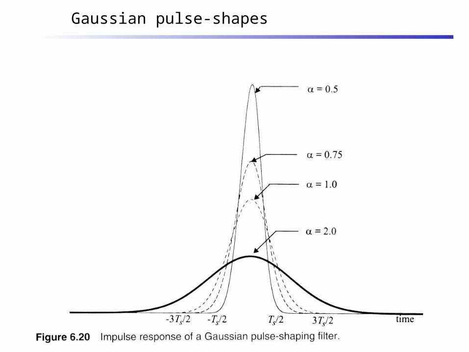
Gaussian pulse-shapes

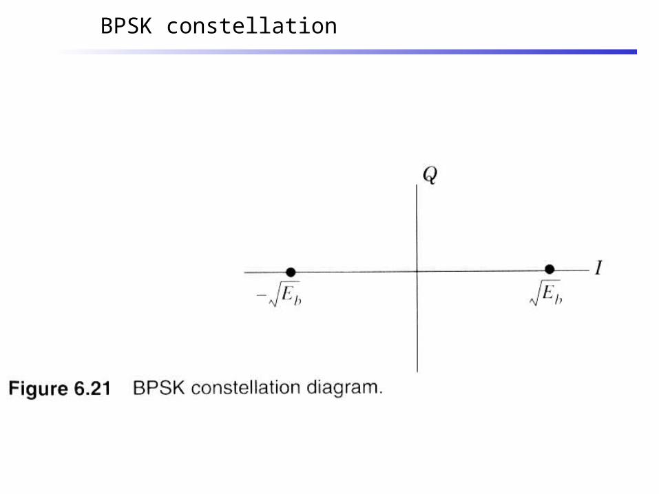
BPSK constellation

Virtue of pulse shaping

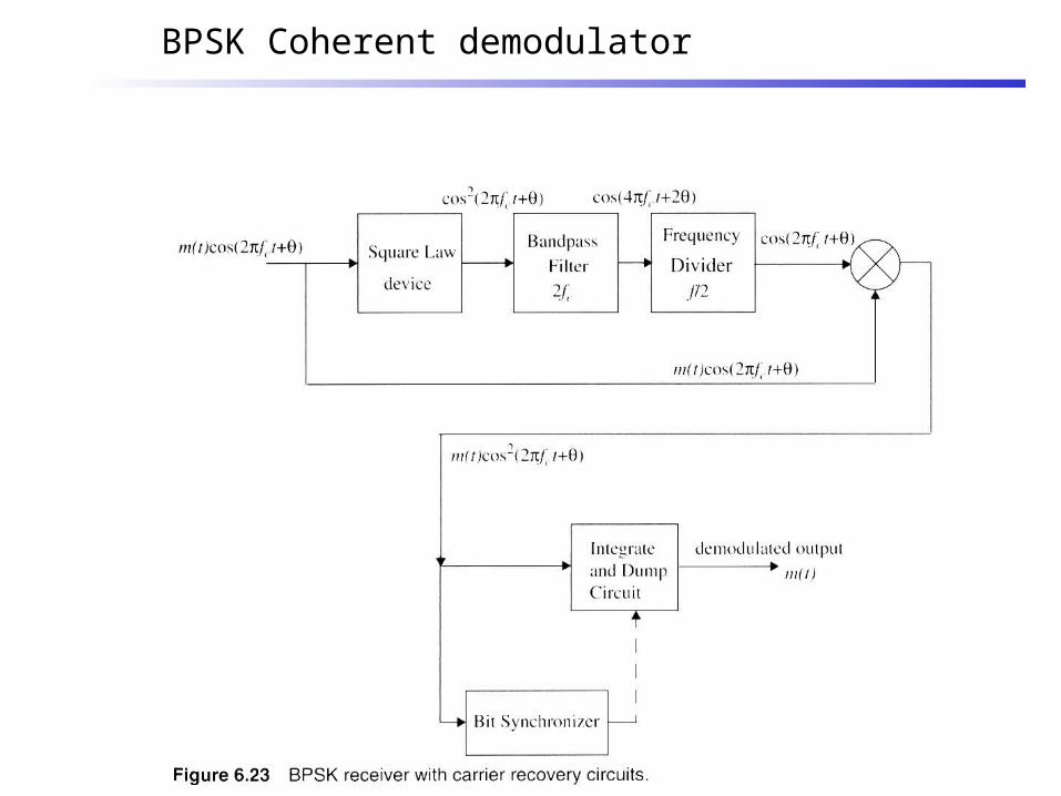
BPSK Coherent demodulator

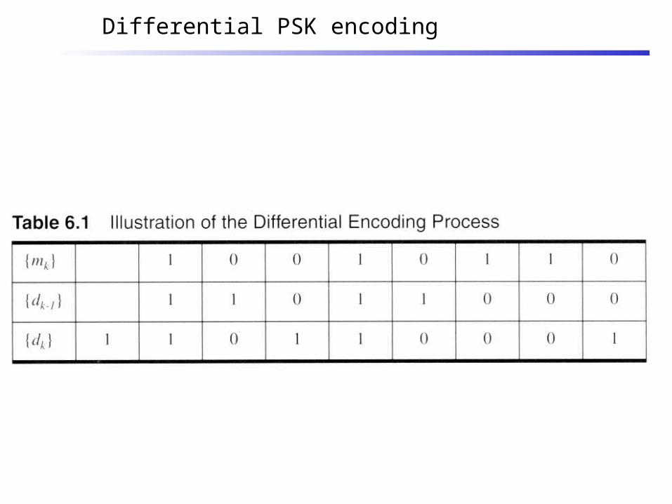
Differential PSK encoding

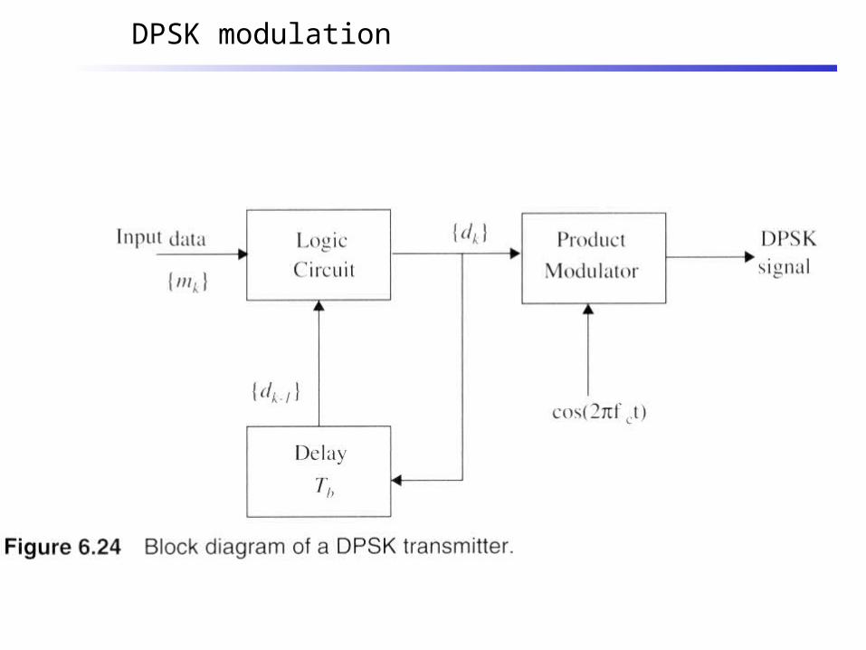
DPSK modulation

DPSK receiver

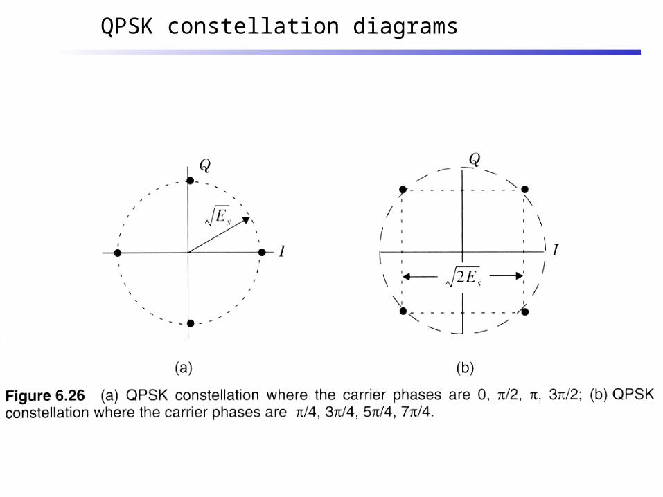
QPSK constellation diagrams

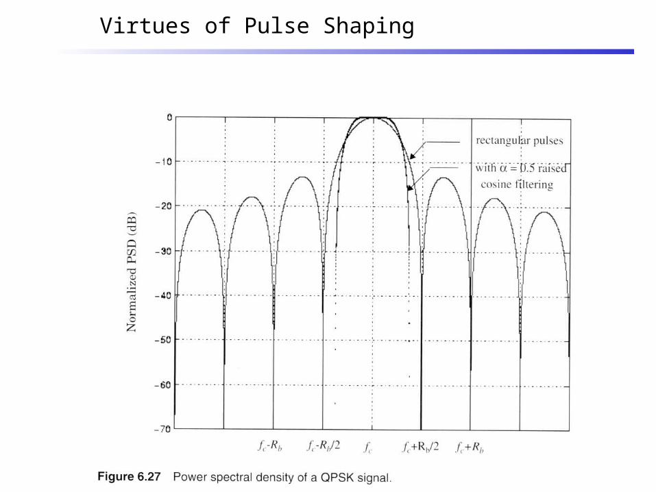
Virtues of Pulse Shaping

QPSK modulation

QPSK receiver

Offset QPSK waveforms

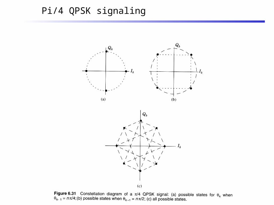
Pi/4 QPSK signaling

Pi/4 QPSK phase shifts

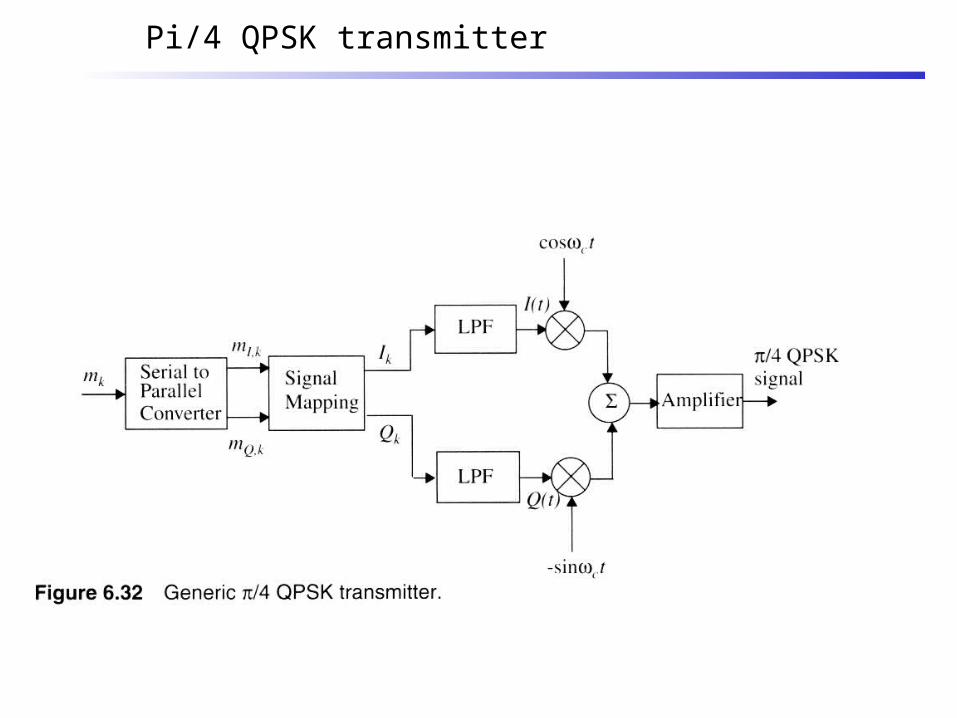
Pi/4 QPSK transmitter

Differential detection of pi/4 QPSK

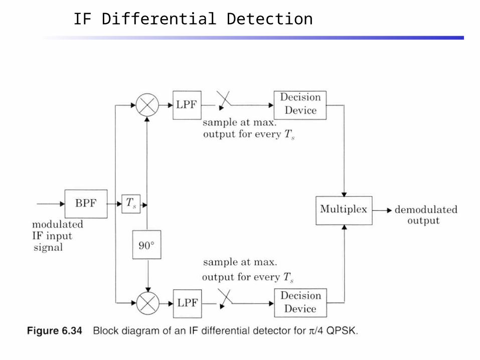
IF Differential Detection

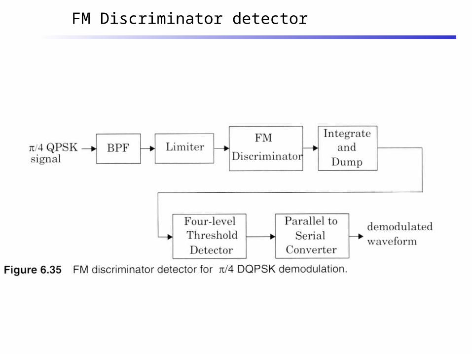
FM Discriminator detector

FSK Coherent Detection

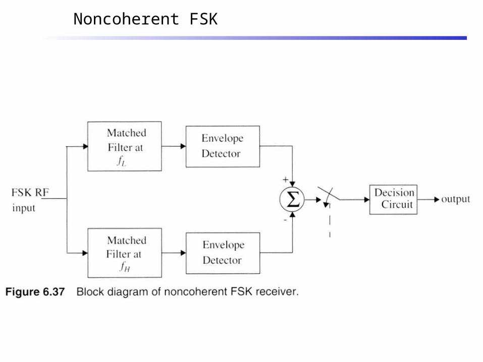
Noncoherent FSK

Minimum Shift Keying spectra

MSK modulation

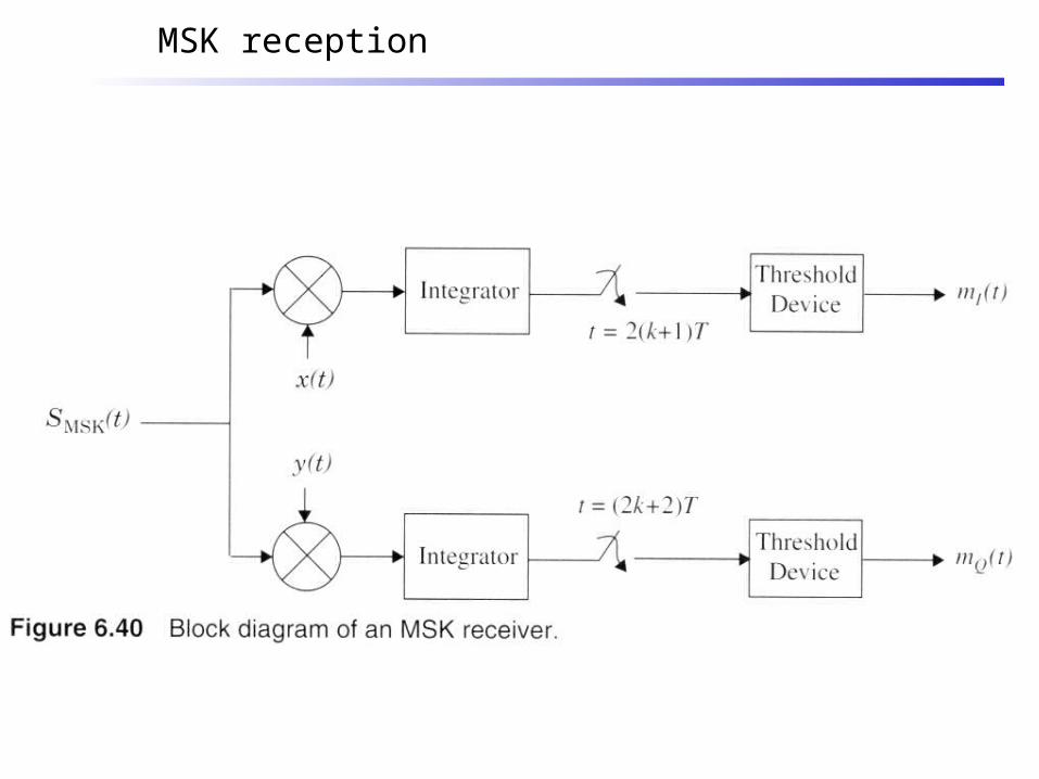
MSK reception

GMSK spectral shaping

GMSK spectra shaping

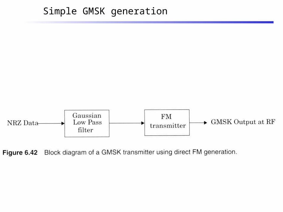
Simple GMSK generation

GMSK Demodulator

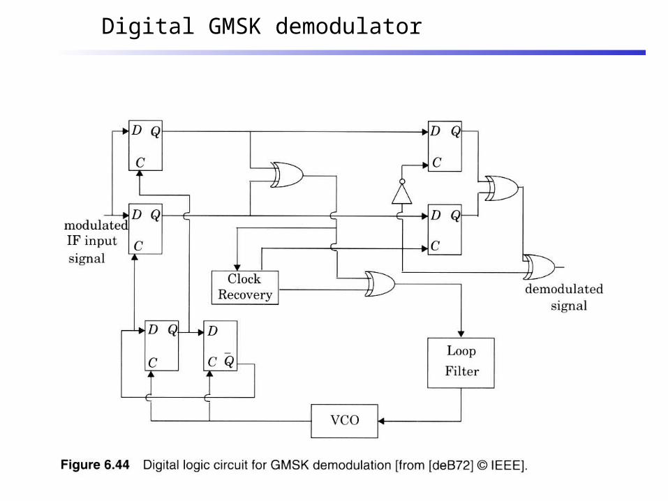
Digital GMSK demodulator

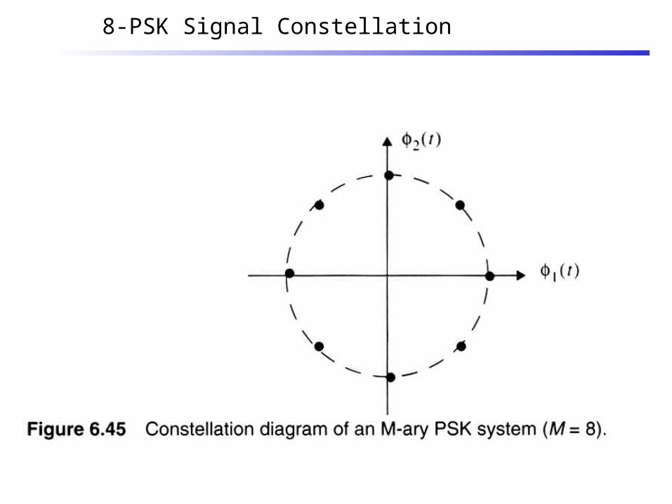
8-PSK Signal Constellation

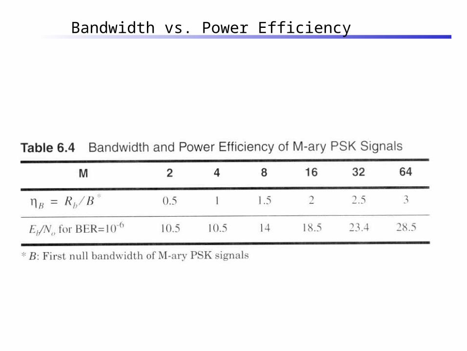
Bandwidth vs. Power Efficiency

Pulse Shaped M-PSK

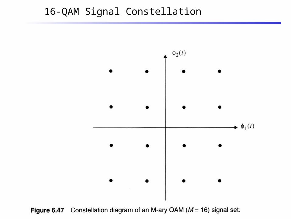
16-QAM Signal Constellation

QAM efficiencies

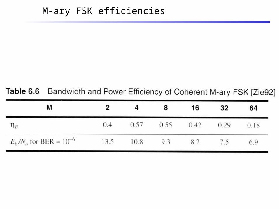
M-ary FSK efficiencies

PN Sequence Generator

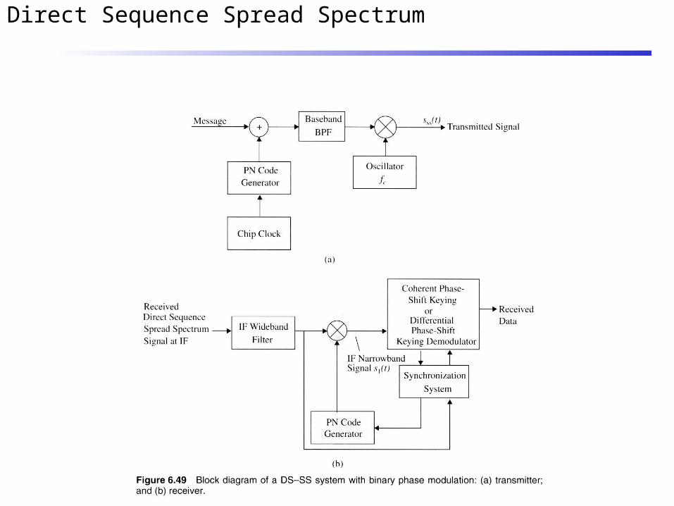
Direct Sequence Spread Spectrum

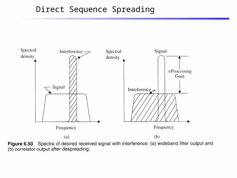
Direct Sequence Spreading

Frequency Hopping Spread Spectrum

CDMA – Multiple Users

Effects of Fading

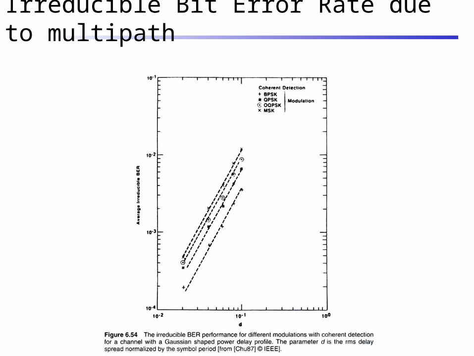
Irreducible Bit Error Rate due to multipath

Irreducible Bit Error Rate due to multipath

Simulation of Fading and Multipath

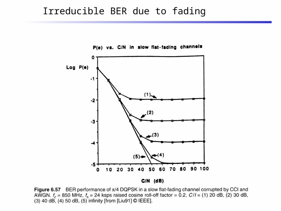
Irreducible BER due to fading

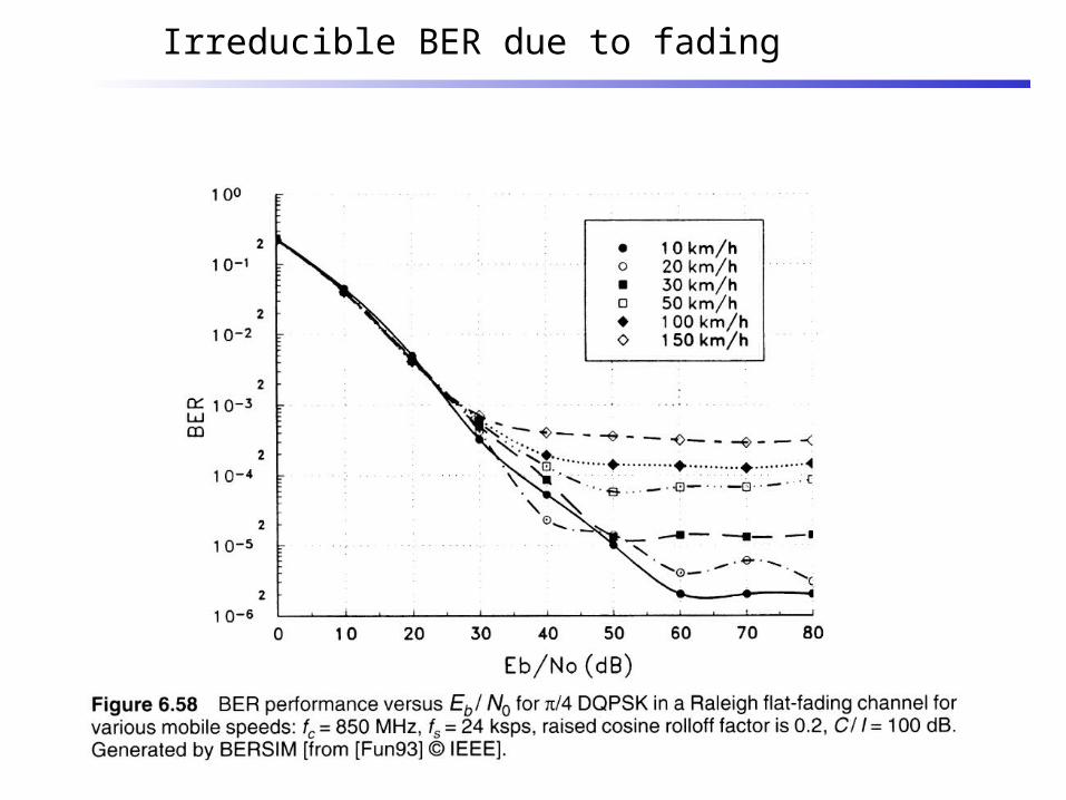
Irreducible BER due to fading

BER due to fading & multipath

137

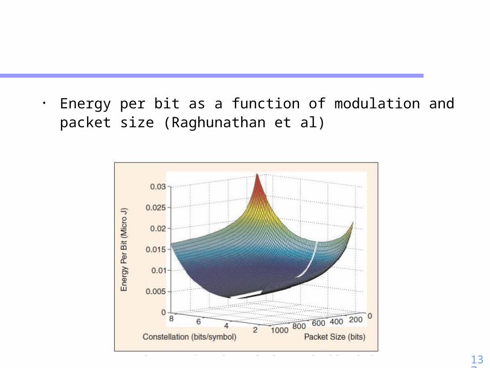
• Energy per bit as a function of modulation and packet size (Raghunathan et al)

138

Slides from Rahul Mangaram

139

Shannon’s Capacity Theorem

• States the theoretical maximum rate at which an error-free bit can be transmitted over a noisy channel

C: the channel capacity in bits per second

B: the bandwidth in hertz

SNR: the ratio of signal power to noise power

• Channel capacity depends on channel bandwidth and system SNR

140

140

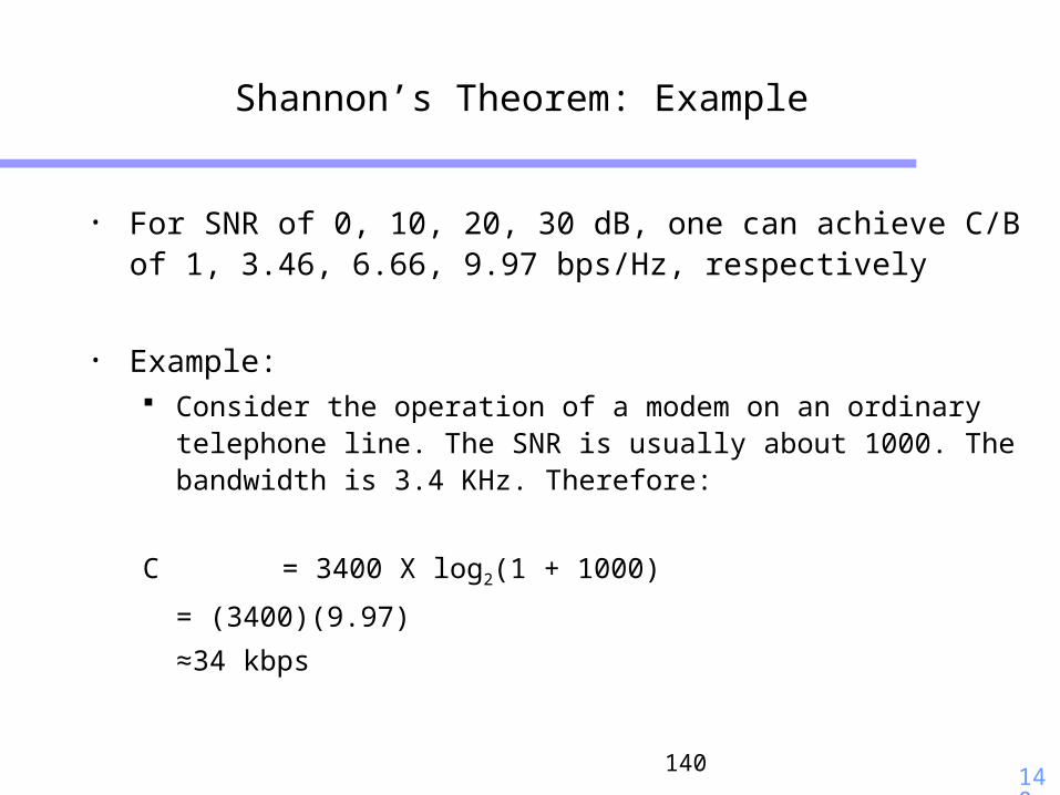
Shannon’s Theorem: Example

• For SNR of 0, 10, 20, 30 dB, one can achieve C/B of 1, 3.46, 6.66, 9.97 bps/Hz, respectively

• Example: Consider the operation of a modem on an ordinary telephone line.

The SNR is usually about 1000. The bandwidth is 3.4 KHz. Therefore:

C = 3400 X log2(1 + 1000)

= (3400)(9.97)

≈34 kbps

141

141

Bit Error Rate

• BER = Errors / Total number of bits Error means the reception of a “1” when a “0” was transmitted or vice

versa.

• Noise is the main factor of BER performance – signal path loss, circuit noise, …

142

142

Thermal Noise

• Thermal Noise white noise since it contains the same level of power at all frequencies kTB, where

k is the Boltzmann’s constant = 1.381e-21 W / K / Hz, T is the absolute temperature in Kelvin, and B is the bandwidth.

• At room temperature, T = 290K, the thermal noise power spectral density, kT = 4.005e-21 W/Hz or

–174 dBm/Hz

143

143

Receiver Sensitivity

• The minimum input signal power needed at receiver input to provide adequate SNR at receiver output to do data demodulation

• SNR depends on Received signal power

Background thermal noise at antenna (Na)

Noise added by the receiver (Nr)

• Pmin = SNRmin ×(Na +Nr)

144

144

Noise Figure

• Noise Figure (F) quantifies the increase in noise caused by the noise source in the receiver relative to input noise

F = SNRinput/SNRoutput = (Na + Nr)/Na

Pmin = SNRmin×(Na + Nr) = SNRmin×F ×Na

Example: if SNRmin = 10 dB, F = 4 dB, BW = 1 MHz Pmin= 10 + 4 -174 + 10×log(106) = -100 dBm

145

145

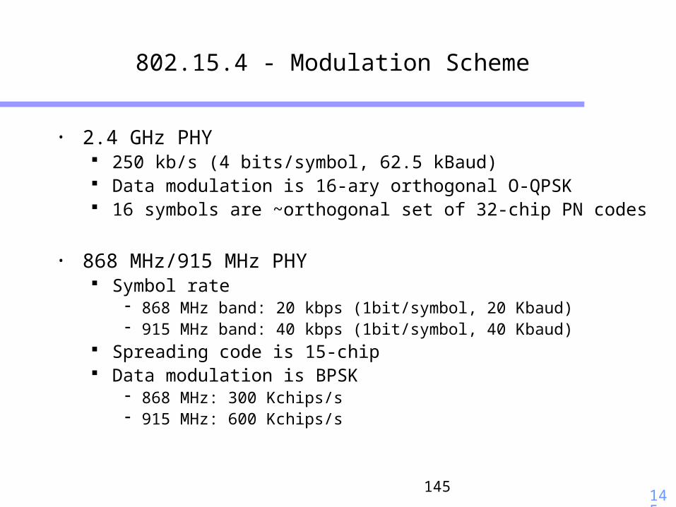
802.15.4 - Modulation Scheme

• 2.4 GHz PHY 250 kb/s (4 bits/symbol, 62.5 kBaud) Data modulation is 16-ary orthogonal O-QPSK 16 symbols are ~orthogonal set of 32-chip PN codes

• 868 MHz/915 MHz PHY Symbol rate

868 MHz band: 20 kbps (1bit/symbol, 20 Kbaud) 915 MHz band: 40 kbps (1bit/symbol, 40 Kbaud)

Spreading code is 15-chip Data modulation is BPSK

868 MHz: 300 Kchips/s 915 MHz: 600 Kchips/s

146

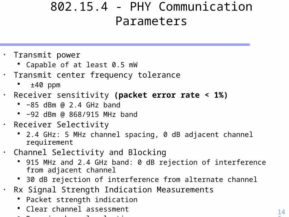
802.15.4 - PHY Communication Parameters

• Transmit power Capable of at least 0.5 mW

• Transmit center frequency tolerance ±40 ppm

• Receiver sensitivity (packet error rate < 1%) −85 dBm @ 2.4 GHz band −92 dBm @ 868/915 MHz band

• Receiver Selectivity 2.4 GHz: 5 MHz channel spacing, 0 dB adjacent channel requirement

• Channel Selectivity and Blocking 915 MHz and 2.4 GHz band: 0 dB rejection of interference from adjacent channel 30 dB rejection of interference from alternate channel

• Rx Signal Strength Indication Measurements Packet strength indication Clear channel assessment Dynamic channel selection

147

147

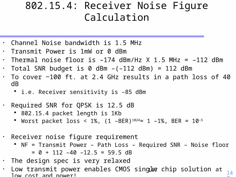
802.15.4: Receiver Noise Figure Calculation

• Channel Noise bandwidth is 1.5 MHz• Transmit Power is 1mW or 0 dBm• Thermal noise floor is –174 dBm/Hz X 1.5 MHz = –112 dBm• Total SNR budget is 0 dBm –(–112 dBm) = 112 dBm • To cover ~100 ft. at 2.4 GHz results in a path loss of 40 dB

i.e. Receiver sensitivity is –85 dBm

• Required SNR for QPSK is 12.5 dB 802.15.4 packet length is 1Kb Worst packet loss < 1%, (1 –BER)1024= 1 –1%, BER = 10–5

• Receiver noise figure requirement

NF = Transmit Power – Path Loss – Required SNR – Noise floor = 0 + 112 –40 –12.5 = 59.5 dB

• The design spec is very relaxed• Low transmit power enables CMOS single chip solution at low cost and power!