2.1 thanks to prof. dr.-ing. jochen h. schiller for the slides mc - 2013 mobile communications...

2.1Thanks to Prof. Dr.-Ing. Jochen H. Schiller for the slides www.jochenschiller.de MC - 2013

Mobile CommunicationsChapter 2: Wireless Transmission

• Frequencies• Signals, antennas, signal propagation• Multiplexing, Cognitive Radio• Spread spectrum, modulation• Cellular systems

2.2

Wireless communications

• The physical media – Radio Spectrum

– There is one finite range of frequencies over which radio waves can exist – this is the Radio Spectrum

– Spectrum is divided into bands for use in different systems, so Wi-Fi uses a different band to GSM, etc.

– Spectrum is (mostly) regulated to ensure fair access

Thanks to Prof. Dr.-Ing. Jochen H. Schiller for the slides www.jochenschiller.de MC - 2013


Frequencies for communication

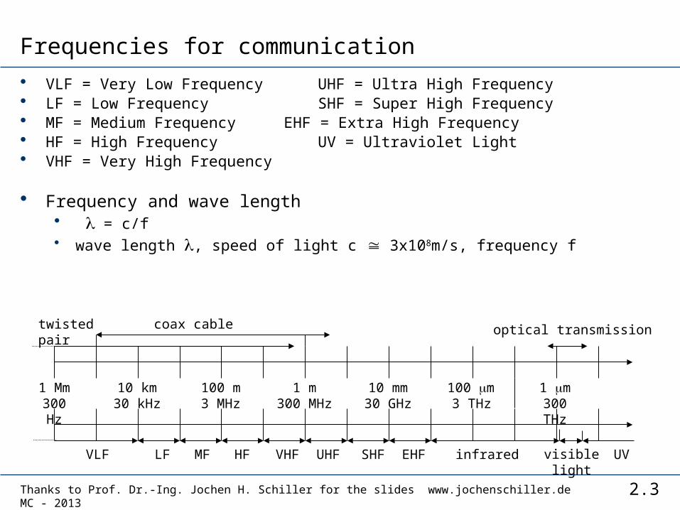
• VLF = Very Low Frequency UHF = Ultra High Frequency• LF = Low Frequency SHF = Super High Frequency• MF = Medium Frequency EHF = Extra High Frequency• HF = High Frequency UV = Ultraviolet Light• VHF = Very High Frequency

• Frequency and wave length• = c/f • wave length , speed of light c 3x108m/s, frequency f

1 Mm300 Hz

10 km30 kHz

100 m3 MHz

1 m300 MHz

10 mm30 GHz

100 m3 THz

1 m300 THz

visible lightVLF LF MF HF VHF UHF SHF EHF infrared UV

optical transmissioncoax cabletwisted pair


Example frequencies for mobile communication

• VHF-/UHF-ranges for mobile radio• simple, small antenna for cars• deterministic propagation characteristics, reliable

connections• SHF and higher for directed radio links, satellite

communication• small antenna, beam forming• large bandwidth available

• Wireless LANs use frequencies in UHF to SHF range• some systems planned up to EHF• limitations due to absorption by water and oxygen molecules

(resonance frequencies)• weather dependent fading, signal loss caused by heavy rainfall

etc.


Frequencies and regulations

• In general: ITU-R holds auctions for new frequencies, manages frequency bands worldwide (WRC, World Radio Conferences)

Examples Europe USA Japan

Cellular networks

GSM 880-915, 925-960, 1710-1785, 1805-1880UMTS 1920-1980, 2110-2170LTE 791-821, 832-862, 2500-2690

AMPS, TDMA, CDMA, GSM 824-849, 869-894TDMA, CDMA, GSM, UMTS 1850-1910, 1930-1990

PDC, FOMA 810-888, 893-958PDC 1429-1453, 1477-1501FOMA 1920-1980, 2110-2170

Cordless phones

CT1+ 885-887, 930-932CT2 864-868DECT 1880-1900

PACS 1850-1910, 1930-1990PACS-UB 1910-1930

PHS 1895-1918JCT 245-380

Wireless LANs 802.11b/g 2412-2472

802.11b/g 2412-2462

802.11b 2412-2484802.11g 2412-2472

Other RF systems

27, 128, 418, 433, 868

315, 915 426, 868


Signals I

• physical representation of data• function of time and location• signal parameters: parameters representing the value of

data • classification

• continuous time/discrete time• continuous values/discrete values• analog signal = continuous time and continuous values• digital signal = discrete time and discrete values

2.7

Signals I

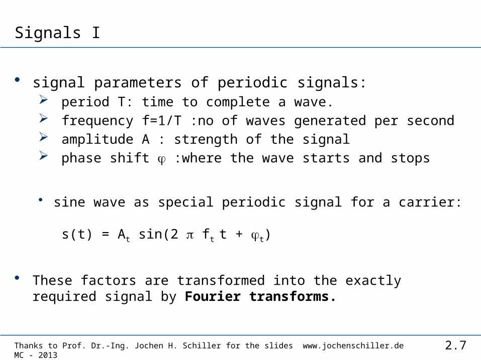
• signal parameters of periodic signals: period T: time to complete a wave. frequency f=1/T :no of waves generated per second amplitude A : strength of the signal phase shift :where the wave starts and stops

• sine wave as special periodic signal for a carrier:

s(t) = At sin(2 ft t + t)

• These factors are transformed into the exactly required signal by Fourier transforms.

Thanks to Prof. Dr.-Ing. Jochen H. Schiller for the slides www.jochenschiller.de MC - 2013


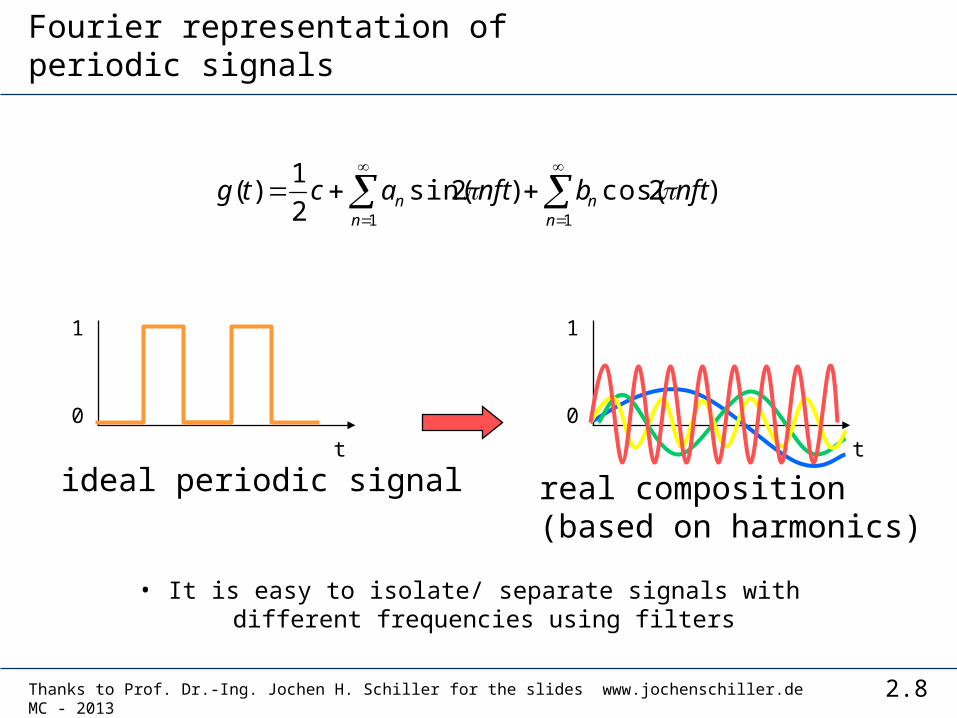
Fourier representation of periodic signals

1

0

1

0

t t

ideal periodic signal real composition(based on harmonics)

• It is easy to isolate/ separate signals with different frequencies using filters

)2cos()2sin(2

1)(

11

nftbnftactgn

nn

n


Signals II

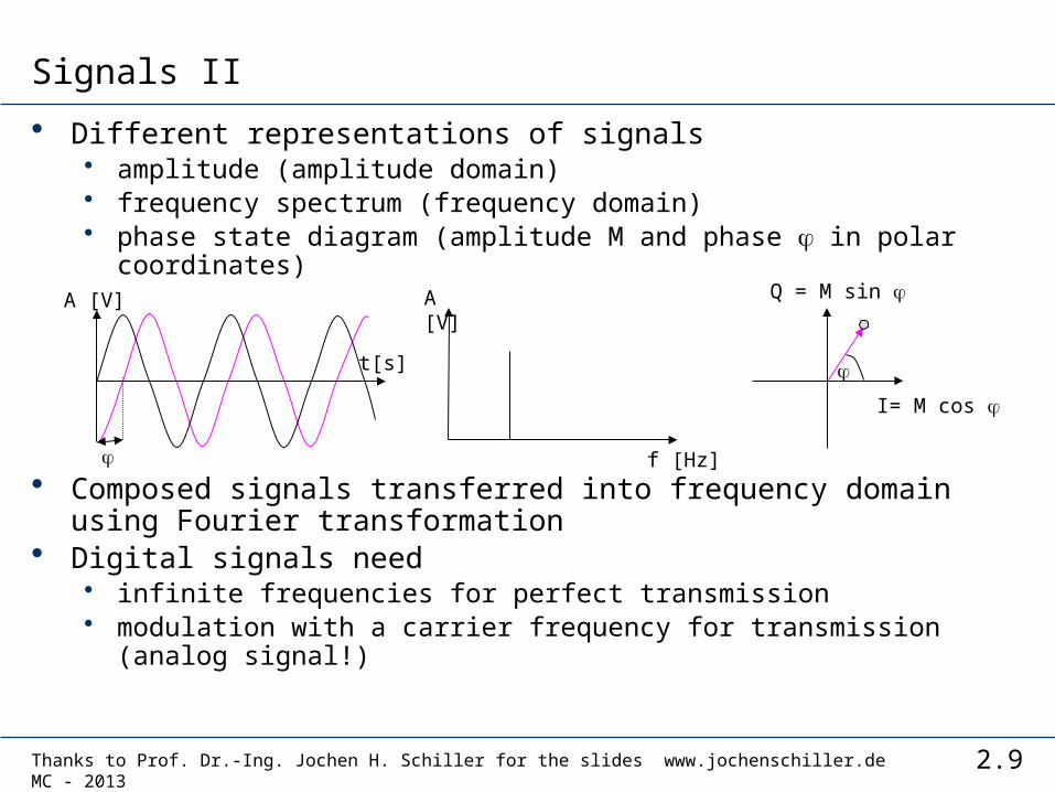
• Different representations of signals • amplitude (amplitude domain)• frequency spectrum (frequency domain)• phase state diagram (amplitude M and phase in polar coordinates)

• Composed signals transferred into frequency domain using Fourier transformation

• Digital signals need• infinite frequencies for perfect transmission • modulation with a carrier frequency for transmission (analog

signal!)

f [Hz]

A [V]

I= M cos

Q = M sin

A [V]

t[s]


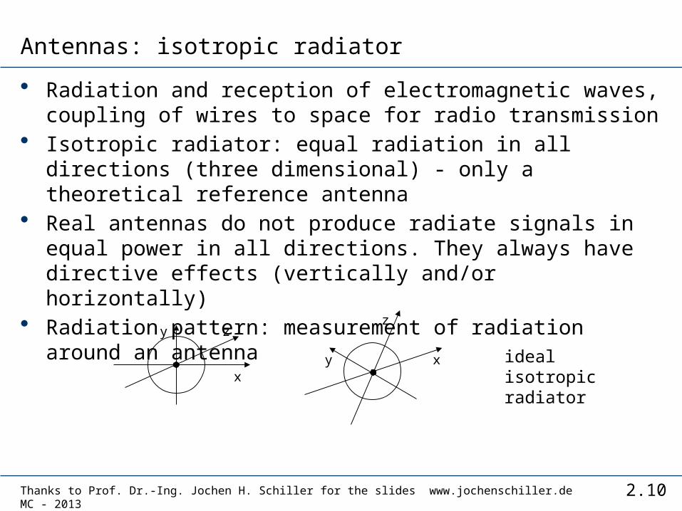
Antennas: isotropic radiator

• Radiation and reception of electromagnetic waves, coupling of wires to space for radio transmission

• Isotropic radiator: equal radiation in all directions (three dimensional) - only a theoretical reference antenna

• Real antennas do not produce radiate signals in equal power in all directions. They always have directive effects (vertically and/or horizontally)

• Radiation pattern: measurement of radiation around an antenna

zy

x

z

y x idealisotropicradiator


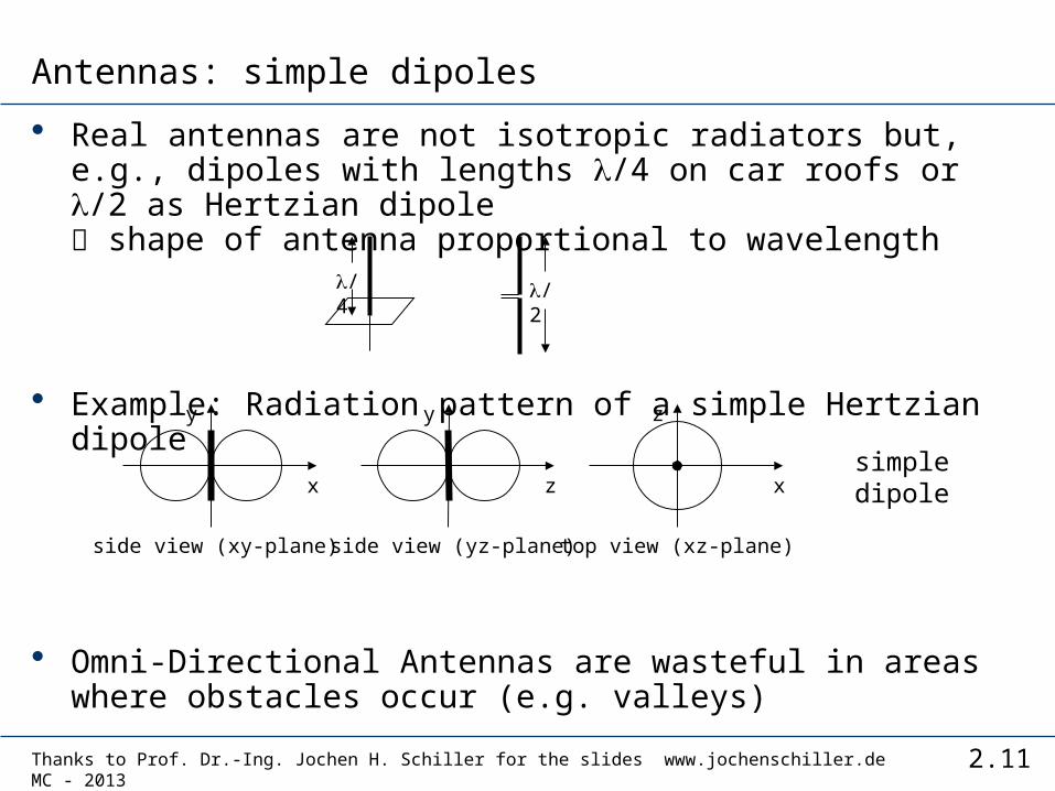
Antennas: simple dipoles

• Real antennas are not isotropic radiators but, e.g., dipoles with lengths /4 on car roofs or /2 as Hertzian dipole shape of antenna proportional to wavelength

• Example: Radiation pattern of a simple Hertzian dipole

• Omni-Directional Antennas are wasteful in areas where obstacles occur (e.g. valleys)

side view (xy-plane)

x

y

side view (yz-plane)

z

y

top view (xz-plane)

x

z

simpledipole

/4 /2


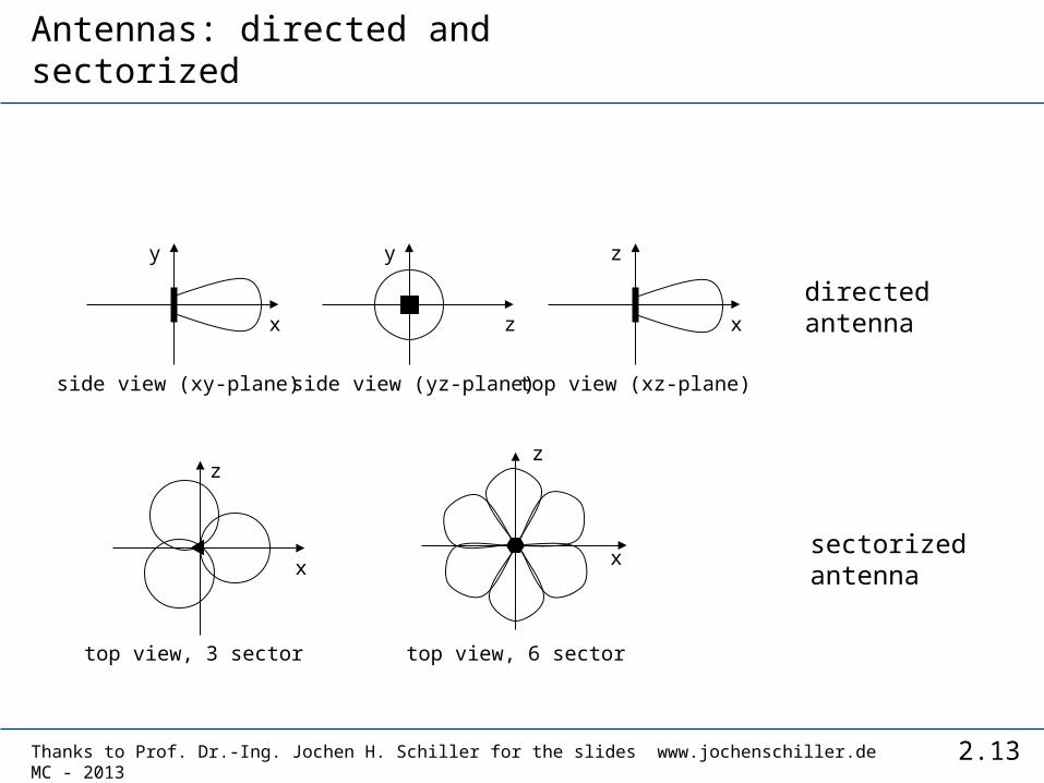
• Directional antennas reshape the signal to point towards a target, e.g. an open street• Placing directional antennas together can be used to form

cellular reuse patterns

• Gain: maximum power in the direction of the main lobe compared to the power of an isotropic radiator (with the same average power)

• Often used for microwave connections or base stations for mobile phones (e.g., radio coverage of a valley)

• Directed antennas are typically used in cellular systems, several directed antennas combined on a single pole to construct Sectorized antennas.


Antennas: directed and sectorized

side view (xy-plane)

x

y

side view (yz-plane)

z

y

top view (xz-plane)

x

z

top view, 3 sector

x

z

top view, 6 sector

x

z

directedantenna

sectorizedantenna


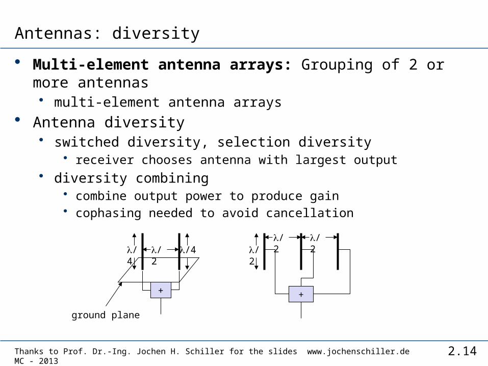
Antennas: diversity

• Multi-element antenna arrays: Grouping of 2 or more antennas• multi-element antenna arrays

• Antenna diversity• switched diversity, selection diversity

• receiver chooses antenna with largest output• diversity combining

• combine output power to produce gain• cophasing needed to avoid cancellation

+

/4/2/4

ground plane

/2/2

+

/2


• Smart antennas use signal processing software to adapt to conditions –e.g. following a moving receiver (known as beam forming), these are some way off commercially

• E.g. wireless devices direct the electro magnetic radiation away from human body toward a base station to reduce the absorbed radiation.


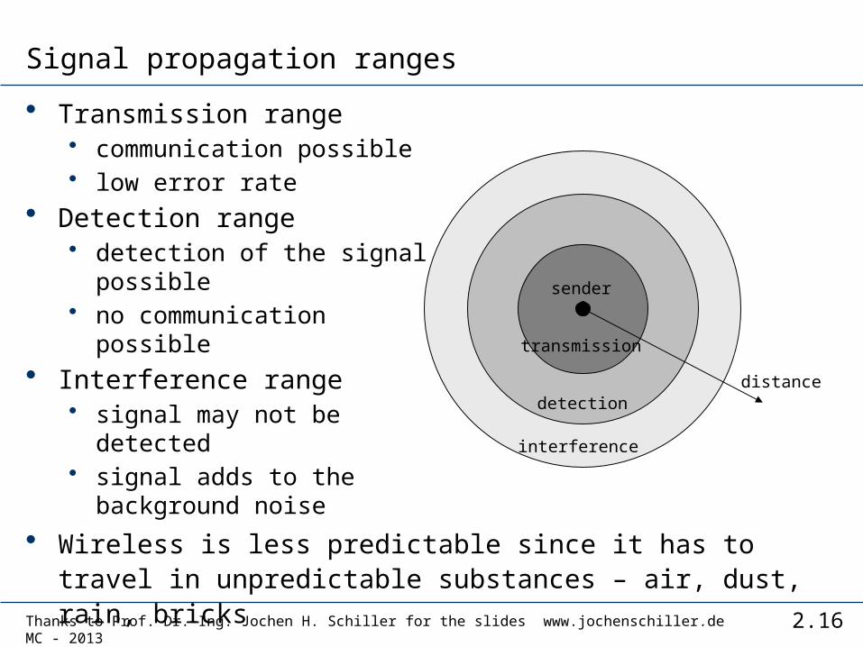
Signal propagation ranges

• Transmission range• communication possible• low error rate

• Detection range• detection of the signal

possible• no communication

possible• Interference range

• signal may not be detected

• signal adds to the background noise

• Wireless is less predictable since it has to travel in unpredictable substances – air, dust, rain, bricks

distance

sender

transmission

detection

interference


Signal propagation: Path loss (attenuation)

• In free space signals propagate as light in a straight line (independently of their frequency).

• If a straight line exists between a sender and a receiver it is called line-of-sight (LOS)

• Receiving power proportional to 1/d² in vacuum (free space loss) – much more in real environments(d = distance between sender and receiver)

• Situation becomes worse if there is any matter between sender and receiver especially for long distances• Atmosphere heavily influences satellite transmission• Mobile phone systems are influenced by weather condition

as heavy rain which can absorb much of the radiated energy


Signal propagation: Path loss (attenuation)

• Radio waves can penetrate objects depending on frequency. The lower the frequency, the better the penetration• Low frequencies perform better in denser materials• High frequencies can get blocked by, e.g. Trees

• Radio waves can exhibit three fundamental propagation behaviours depending on their frequencies:• Ground wave (<2 MHz): follow the earth surface and can

propagate long distances – submarine communication• Sky wave (2-30 MHz): These short waves are reflected at the

ionosphere. Waves can bounce back and forth between the earth surface and the ionosphere, travelling around the world – International broadcast and amateur radio

• Line-of-sight (>30 MHz): These waves follow a straight line of sight – mobile phone systems, satellite systems


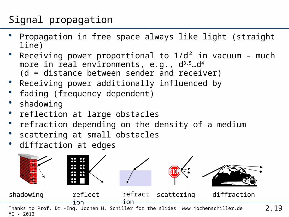
Signal propagation

• Propagation in free space always like light (straight line)• Receiving power proportional to 1/d² in vacuum – much more in

real environments, e.g., d3.5…d4

(d = distance between sender and receiver)• Receiving power additionally influenced by• fading (frequency dependent)• shadowing• reflection at large obstacles• refraction depending on the density of a medium• scattering at small obstacles• diffraction at edges

reflection scattering diffractionshadowing refraction


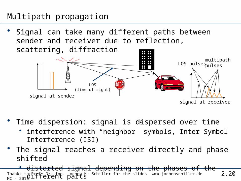
Multipath propagation

• Signal can take many different paths between sender and receiver due to reflection, scattering, diffraction

• Time dispersion: signal is dispersed over time• interference with “neighbor” symbols, Inter Symbol

Interference (ISI)• The signal reaches a receiver directly and phase shifted

• distorted signal depending on the phases of the different parts

signal at sendersignal at receiver

LOS pulsesmultipathpulses

LOS(line-of-sight)


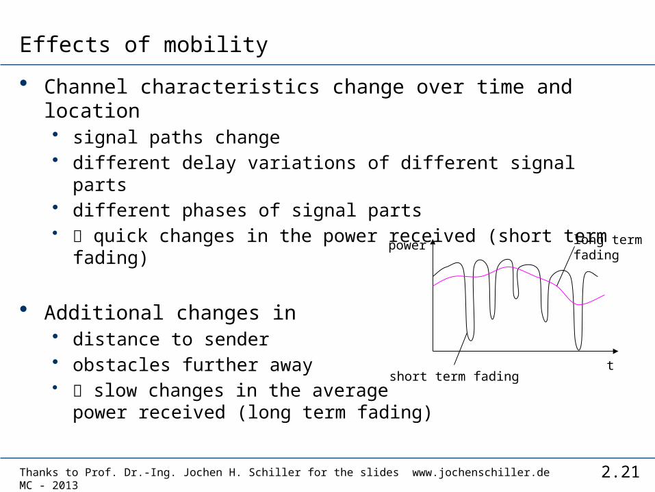
Effects of mobility

• Channel characteristics change over time and location • signal paths change• different delay variations of different signal parts• different phases of signal parts• quick changes in the power received (short term fading)

• Additional changes in• distance to sender• obstacles further away• slow changes in the average

power received (long term fading)

short term fading

long termfading

t

power

2.1 thanks to prof. dr.-ing. jochen h. schiller for the slides mc - 2013 mobile communications...

Documents

high frequency frequency

radio spectrum spectrum

high frequency lf

high frequency uv

high frequency hf

low frequency shf

new frequencies

example frequencies