It This Nsea:Nh lA1aS sUPP01'ted by the Office of Naval Reseazteh under contractN00014-6?-A-0321-0002.

PoINT Pro:Esses GeNERATED BY lEvEL CRossINGS

M. R. Leadbetterlt

Department of StatisticsUniversity of North Carolina at ChapeZ Hi'Ll

Institute of Statistics Mimeo Series No. 764

July, 7971

PoINT PRlCESSES GENERATED BY lEvEL CRosSINGS

by

M. R. Leadbetter*University of North Carolina at Chapel, HiH

s~

This paper consists primarily of a review of available literature (and

especially more recent work) concerning the crossings of levels and curves by

stochastic processes. Attention is particularly directed towards those prop-

erties for which it is most profitable to emphasize the point process nature

of the crossings. Topics considered include the mean and moments of the number

of crossings, the distributions of times between them, "crossings" by vector

processes and fields, Poisson approximations, and local extremes with parti-

cular reference to "crest-trough" times and heights.

I. INTROWCTION

The problems concerning crossings of levels and curves by stochastic pro-

cesses are very closely related to a number of areas of stochastic process

theory. Such areas include local properties (continuity, etc.) of stochastic

process sample functions, extreme value theory of stochastic processes, and

This research was supported by the Office Of Naval, Research undercontract N00014-6?-A-0321-0002.

2

the theory of point processes (cf. [14]). While other aspects must necessarily

enter, it is the latter connection - the particular emphasis on purely point

process properties - which we wish es)ecially to develop in this paper. The

selection of topics reflects this interest and has resulted in the exclusion

of some problems which might have been treated.

Within this framework, the aim of the paper is to review the currently

available literature on a spectrum of level- and curve- crossing problems,

with particular reference to recent work. The historical references will be

largely confined to this introductory section and the summary of the contents

of the paper given below. A much fuller discussion of work up to 1967 may be

found in [14].

The interest in crossing problems really dates back to the original papers

of M. Kac [20] in 1943 and S. O. Rice [41] in 1945. In particular, Rice ob-

tained the now familiar formula for the mean number EC of crossings of a level

u by a stationary (zero mean) stochastic process ~(t) in an interval

o ~ t ~ T viz.

(1.1) EC

where if ret) denotes the covariance function of ~(t), AO = reO) = v~~(t)

and A = -r"(O) ,2

the second derivative of r at the origin. is also

the "second spectral moment", AZ = fA 2dF(A) if F denotes the spectral

function for ~(t).)

The conditions under which (1.1) holds were successively weakened by

various authors, including Ivanov [19], Bulinskaya [11], Ito [18] and

Ylvisaker [42], the latter two authors giving minimal conditions. In parti-

cular, Ylvisaker used a counting procedure for the number of zeros which may

be readily adapted to a general point process framework. This will be discussed

3

in Section 2 following the definition of terms concerning crossings and a

description of the previous counting procedures used (following Kac).

In Section 2 and throughout the paper, we shall mainly think in terms of

upc!'Ossings of levels, rather than all crossings, for reasons of "cleanliness"

of exposition in the later sections. The modifications required to deal with

downcrossings or all crossings will be evident. The notation N(a,b) will

be used in two senses: first to denote the number of upcrossings of some

fixed level (or curve) in the interval a < t S b, and also to denote the num-

ber of events of an arbitrary point process in that interval. It seemed pre-

ferable to do this to avoid duplicating notation, since it will always be clear

which use is intended, and the first use is, of course, a special case of the

second. In later sections, we will need also to use the notation N (a,b)u

where the level u considered will be changing.

Section 3 contains applications of the general results of Section 2. The

standard results for crossings of levels and curves by normal (stationary and

non-stationary) processes are given and a general result for non-normal pro-

cesses, including, in particular,application to the envelope of a stationary

normal process. This section is concluded with some recent general results of

Fieger concerning the generalization of the crossing framework to include pos-

sibly discontinuous curves and sample paths.

The higher (factorial) moments of the number N(O,T) of upcrossings are

considered in Section 4. Again a general point process framework is used in

which the kth factorial moment of N(O,T) is exhibited as the mean number of

thevents of a process, the "k derived process", formed from the original one

but in k-dimensional Euclidean space Rk • This follows essentially the treat-

ment of the problem by Belayev [s]. The specific methods used for obtaining

the moments are indicated from this basic viewpoint. Questions of finiteness

of the moments are briefly mentioned.

4

One of the main uses of the factorial moments of the number of upcros­

sings of a level in a given time, is to describe the distribution of the time

between successive upcrossings by a stationary normal process. Series ex­

pressions of which one was given by Rice [41] and many more, later by Longuet­

Higgins [32], may be given for such distributions. It turns out that the terms

in the series are in fact (derivatives of) the factorial moments.

Again these are special cases of results which hold for in a much wider

framework - that of stationary point processes. This is described in Section

5, from which the specific application to the intervals between say upcros­

sings amy be obtained. The cOncept of a "mixture" of point processes is also

mentioned in that section - leading in particular to the distribution of the

length of, say, an upwards excursion of a level u (i.e., the time from an

upcrossing to the next downcrossing).

In Section 6, we consider generalizations of crossing problems to in­

clude vector processes and fields. Specific results are described and it is

shown that these are typically special cases of a crossing of a fixed vector

by a "vector field", or equivalently the solutions of n random equations in

n unknowns.

The behaviour of a sequence of stationary point processes on the line,

with intensities tending to zero, tends to take on more and more a Poisson

character in certain cases. The important application for our purposes here

concerns the upcrossings of an increasingly high level by a normal stationary

process. (In particular, this leads to the asymptotic distribution of the

maximum of such a process.) These questions are discussed in Section 7.

The final topic of the paper - in Section 8 - concerns the occurrence of

local extremes of a stationary normal process. In particular, we indicate

some interesting recent work of G. Lindgren [29] on the behaviour of such a

5

process near a local maximum and the asymptotic properties of crest-trough

times and heights.

2. THE POINT PROCESS OF LEVEL CROSSINGS. CoUNTING PROCEDURES FOR THE MEAN

NlJttBER OF EVENTS.

In this section, we shall review the basic theory for calculation of the

mean number of crossings of a level by a stochastic process, including the

original "counting procedure" due to Kac [20], and the now more often used

method due to Y1visaker [42]. This latter procedure will be cast here within

a point process framework. Specific applications will be given in the next

section.

It will be assumed throughout this section that the process ~(t) con­

sidered has continuous sample functions (see, e.g. [14] for a variety of suf­

ficient conditions for this to hold). The relaxation of the continuity con­

dition will be considered in the next section.

Following [14,§lO.2], we say that ~(t) has an uparossing of the level

u at to if for some £ > 0, ~(t) S u for t o-£ < t < to' and ~(t) ~ u

for to < t < t o+£. Downcrossings are defined by simply reversing the in­

equalities ~(t) S u, ~(t) ~ u, whereas ~(t) has a arossing of the level

u at to if in each neighbourhood of to there are points t l , t 2 with

(~(tl)-u)(~(t2)-u) < O. (For a discussion of these definitions, we refer to

[14,§lO.2] •

To obtain the mean number of, say upcrossings, of u in an interval I,

it is necessary to approximate the number of upcrossings as the limit of a

sequence of quantities whose means can be calculated from the process distri­

butions. (This point will be developed further in relation to a general point

process later in this section.) For example, Kac [20] used a counting procedure

6

of the form

in which ~+'(t) is the derivative ~'(t) of ~ where this is non-negative,

and zero otherwise, and o (.)n

is a sequence of functions "becoming more like

a o-function" as n increases (e.g., o (x) • n for Ixl s 1!2n, 0 (x) • 0n n

otherwise). That W approximates the number N(I)n

of upcrossings of u by

~(t) in I may be seen intuitively by regarding I as being composed of

disjoint intervals in each of which ~'(t) has constant sign. The integrand

vanishes on the intervals on which ~'(t) S 0 and on each of the other inter­

vals may be transformed to give a contribution /a 0 (v)dv where a < 0 < aa n

For such intervals

"counts" the number of upcrossings of

if and only if that interval contains an upcrossing.

lao (v)dv ~ 1 whereas for the others (with a < 8 < 0a n

/80 (v)dv ~ O. Thus in the limit Wann

or o < a < e)

u by ~(t) in I. The mean number of upcrossings is then obtained as

Urn Ew.n+co n

Later authors (e.g., [19], [11], [21]) followed Kac in using similar

counting procedures. More recently, it has become customary to use a very

simple and in some ways more natural procedure (due to Ylvisaker [42]) which

does not (at least explicitly) make any differentiability assumption necessary.

It does, however, appear that the "Kac counting procedure" may provide a

rather useful and natural method of dealing with certain crossing problems

for vector processes (see Section 6).

Instead of describing the counting procedure used by Ylvisaker directly,

we give a modified general version within a purely point process framework.

This, we feel, provides an illuminating viewpoint and is certainly relevant

to the aims of the present paper. Specifically, the following result holds.

7

(We shall consider the interval (0,1] fo~ simplicity - the required alter-

ations for any other interval will be obvious.)

Theorem 2.1. Consider a point process without multiple events and let

N(s,t) • N(I) denote the number of events in the semiclosed interval

(s,t] = I. Divide the interval (0,1] into n sub-intervals

Ini = «i-l)/n, i/n], i· 1,2, ••• ,n, n = 1,2, ••• Then

(2.1) EN(O,l) • U.mn-+ oo

nI Pr{N(Ini) ~ I}.

i-I

The proof of (2.1) is obtained very simply by writing Xni - 1 if

nN(Ini) ~ 1, Xni • 0 otherwise and Nn - Li _l Xni ' Then it is clear that

N -+ N(O,l) with probability one, and hence by Fatou's lemma, sincen

N ~ N(O,l), it follows that EN -+ EN(O,l) S 00, from which (2.1) follows.n n

It may be noticed that this argument can be regarded also as the heart of

simple proofs of (a) the equivalence of the "principal" and "parametric" mea-

sures of a point process on the line ("Korolyuk's Theorem" - cf. [5]) and

(b) the expression of EN(O,l) as the "Burkill integral" f~ P{N(') ~ l}

(cf. [16]).

Equation (2.1) expresses the mean number of events in the interval (0,1]

in terms of distributions of numbers of events in (small) intervals. If the

events are, say, upcrossings of a level by a process ~(t), we wish to ex-

press EN(O,l) in terms of the finite-dimensional distributions of ~(t). It

is intuitively clear that we should be able to replace Pr{N(Ini) ~ I} in

(2.1) by Pr{~«i-l)/n)<u<~(i/n)} in such a case. Specifically, we have the

following result.

Theorem 2.2. Let ~(t) be a stochastic process whose sample functions

are continuous with probability one, and such that for the given level u,

8

Pr{~(t)=u} = 0 for all t. Then if N(s,t) N(I) denote the number of up-

crossings of u by ~(t) in I = (s,t], it follows that

(2.2) EN(O ,1) = < u <

This result may be proved from Theorem (2.1) by defining Xni as in the

proof of that theorem and Xni, = 1 if ~«i-l)/n)<u<~(i/n), Xni

, = 0

otherwise. Clearly N , n , < rn and hence Urn -6UP EN '= rial Xni Xni:S

n - i=l n

EN(O ,1) by Theorem 2.I. But it is apparent that with

probability one for n fixed, N :S N 'n m when m is sufficiently large, since

then an upcrossing of u in «i-l)/n, i/n) implies ~«j-l)/m)<u<~(j/m) for

some subinterval

and hence

of Thus, by Fatou's lemma, lim ~n6 EN ' ~ ENm m n

lim ~n6 EN 'mm

~ tim ~n6 EN = EN(O,l)n

n(Theorem 2.1)

showing that EN ' ~ EN(O,l), which yields (2.2).n

Thus the calculations of the mean number of upcrossings in an interval is

better carried out by substituting the simpler event "~ «i-I) In) <u<F; (i/n) II

for IlN«i-l)/n, i/n) ~ I". This is rather obvious and indeed it is easy to

proceed directly to Theorem 2.2 without using Theorem 2.1.

The mean number of downcrossings of the level u in (0,1) is, of

course, obtained under the same conditions by reversing the inequalities in

(2.2), whereas the mean number of crossings is obtained by adding the results

for upcrossings and downcrossings.

These results may be applied at once to give the standard formulae for

normal and other processes. Such applications are noted in the next section.

To conclude this section, we mention that the above method for calculation the

mean number of events from a simpler result such as (2.2) rather than (2.1)

9

may be given considerable generality. Such very general considerations have

been given by Fieger [16] in a related, but differently organized framework.

We shall use a somewhat less general and simplified version of what Fieger

terms an "aussch6pfend" set function [16,§3], designed to handle standard ap-

plications.

Specifically, let (n, F, P) denote the basic probability space on which

a given point process is defined. For each n = 1,2 ••• i = O,±I,±2 •••

let Sni = S(Ini ) be an F-measurable set determined by the interval

Ini • «i-l)/n, i/n]. Then Sni will be called a sufficient set fUnction for

the point process if for each n, i,

and

(a) c

(b) with probability one, if N (I i) ~ 1,(jJ n

there exists an integer

m •o such that for any m ~ rnOan integer j may be found

with (jJ € Smj and I mj C I ni •

Theorem 2.2 may then be generalized as follows.

Theorem 2.3. Let Sni be a sufficient set function for the point pro­

cess considered in Theorem 2.1. Then

nf{N(O,l)} • tim l P(Sni)'

n -+ co i-I

(cf [16]).

3. APPLICATIONS AND GENERALIZATIONS

For a stationary process ~(t) satisfying the conditions of Theorem 2.2,

we have at once, for the intensity fN(O,l) of up crossings of the level u:

(3.1) EN(O,l) . -1 -1= lim Pr{~(O) < u < ~(n )}/n •n~+"'co

10

In the case of a stationary normal process (zero mean, unit variance, co-

variance function r(t», this easily yields the familiar formula of Rice [41]

viz. ,

( 3.2)

where A2 is the "second spectral moment" taking the value -r"(O) if r is

twice differentiable, and +~ otherwise. The mean number of downcrossings of

u in 0 ~ t ~ 1 has the same value and the mean number of crossings, twice

the value given by (3.2).

For a non-stationary normal process ~(t) the mean number of upcrossings

of the ze1'o level in 0 ~ t ~ 1 may be similarly obtained and has the ex-

pression

(3.3)

in which (if ~(t) has mean m = m(t) and covariance function r(t,s»,

II =

n =

r(t,t) y =

[ar(t,s)/aS]s=t/ (yo)

[dm _ Yllm/o]/{Y(1-ll2)~}dt

it being assumed that dm/dt and a2r(t,s)/at<ls are continuous functions and

that 0 > 0, Illi < 1 for each t. $ is the standard normal density (With cl.f.

~). A discussion of this result, and details of proof, are contained in

[14,§13.21. While it applies to upcrossings of ze1'o, it can be modified to

apply to any level u by simply writing m(t)-u for met) (since ~(t)-u

is a normal process with mean m(t)-u and covariance function r(t,s) which

crosses zero whenever ~(t) crosses u). Indeed, we may clearly consider up-

crossings of a (continuously differentiable) curve u(t) (defined to be

11

upcrossings of zero by ~(t)-u(t» by simply writing m(t)-u(t) in place of

met) in (3.3).

Another way of writing (3.3) is

(3.4)

where Pt(x,y) denotes the joint density for the normal process ;(t) and its

q.m. derivative ;'(t). In fact, this result holds for a wide variety of sto-

chastic processes ~(t) - not necessarity stationary or normal. A variety of

conditions are possible to ensure (3.3) for an arbitrary process. Those in

the following theorem - given in [22] - are sometimes useful.

Theorem 3.1. Let ~(t) be a stochastic process with continuous sample

functions and joint density f t (x,y) for ~(t), ~(s), t; s. Write,s

(i.e., the joint density for ;(t) and

[;(t+T)-;(t)]/T). Assume that ~(t) and its q.m. derivative ;'(t) have a

joint density Pt(x,y). Then the following three conditions imply the truth

of Equation (3.4):

(i) gt,T(x,y) is continuous in (t,x) for each y, T

(ii) gt,T(X,y) ~ Pt(x,y) as T ~ 0 uniformly in (t,x) for each y

~ hey)00

(iii) gt,T(X,y) for all t, T, x, where 10

yh(y)dy < 00.

Equation (3.3) for normal processes, may be obtained from Theorem 3.1. As

another application we mention the upcrossings of a level u by the enveZope

R(t) of a stationary normal (zero mean, unit variance) stochastic process

;(t), defined (cf. [14]) to be

where if ~(t) has the spectral representation

12

~(t) .. I: CO~ At dU(A) + I: ~~n At dV(A),

~(t) is its Hilbert transform, defined by

~(t) .. I: ~~n At dU(A) - I: CO~ At dV(A).

Application of Theorem 3.1 yields, after calculation,

(3.5) EN(O,l) .. (6/2~)~ u eXp(-u2/2)

in which 6 is a constant determined by the first two spectral moments AI'

A2

of ~, 6" A2

-A1

2 (Ai"!~ AidF(A) if F denotes the "real form" of

the spectrum of ~). The details of this calculation may be found in [22].

We will describe another method for obtaining this result in Section 6.

Our final topic in this section concerns the possibility of relaxing the

requirement of sample function continuity. As far as stationary no~aZ pro-

cesses are concerned, the question is of little importance since it is known

([2])that for a stationary normal process if the sample functions are not con-

tinuous with probability one, then they are unbounded (above and below) in

every finite interval. Thus in this case, one should certainly regard the

number of crossings of a level as being infinite with probability one. This

combined with Equation (3.2) (with the value m if AZ " m) describes the

mean number of (up)crossings for a stationary normal process in all

circumstances.

On the other hand, for other types of discontinuous processes, it may be

of interest to obtain the mean number of crossings of a level. A result of

this type could then be used also to calculate the mean number of crossings of

a possibly discontinuous curve by a process with continuous or discontinuous

sample paths.

13

Fieger [16] has recently investigated this problem in considerable gen-

erality. He uses a slightly different definition of crossings and upcrossings

from ours - especially relative to the endpoints of the interval considered,

and obtains an equation like (2.2), expressed as a Burkill integral. For a

normal process ~(t) (not necessarily stationary), Fieger is then able to

give necessary and sufficient conditions for finiteness of the mean number of

crossings of a level in a given interval. Temporarily using his notation, in

which m(a,b;g) denotes the number of crossings (computed according to his

definition) of the curve g(o) in the interval with endpoints a, b, Fieger

obtains the following result.

Theorem 3.2 (Fieger). If ~(t)-g(t) is separable, ~(t) being normal

with zero mean, unit variance and covariance function ret,s) then tm(a,b;g)

exists if and only if

(a) get) is of bounded variation on [a,b]

and

~)b k

f [l_r(o,o)]2 exists as a Burkill integral.a

The formula for the mean number of crossings also appears compactly in

this framework ° Specifically, Fieger defines a function Set) as the Burkill

integral ft[l-r("o)]~ and gives a formula for the mean number tm(a,b;y)a

of crossings of a level y by the (same) normal process ~(t) in the inter-

val with endpoints a, b. t~en S(o) is a continuous function this becomes

(3.6) tm(a,b;y) • (2~/~) exp(-y2/2) fb [l-r(o,o)]~.a

2For a 8tatio~ normal process for which l-r(t,s) - ~A2(t-s) (i.e., with

second spectral moment A2) the Burkill integral f~[l-r(o,o)]~ clearly be­

comes (A2/2)~(b-a) which gives

tm(a,b;y) = (A2~/~) exp(-y2/2) (b-a)

14

(consistently with (3.2) in view of the difference between arossings and up-

crossings). If A2 = ~ this again gives Em(a,b;y).~.

Equation (3.6) is a pleasant and very compact way of expressing the mean

number of crossings of a level. Of course, in particular cases one would still

need to make assumptions about the behaviour of r(t,s) (such as those leading

to (3.3» in order to evaluate the Burki11 integral lb[l-r(o,.)]~a

4. r1>f>£NTS OF TIiE NUt-BER OF CROSSINGS

Again, to be definite, we shall consider uparossings of a level u by

the stochastic process ~(t) and write N(s,t) for the number in (s,t]. One

is interested in the moments of the random variables N(s,t) for at least two

reasons. First, since the distributions of these random variables are usually

unknown the moments are helpful quantities to calculate particularly if limiting

results of some kind are of interest. Second - as discussed further in the

next section - knowledge of the moments permits a calculation (even though it

may be comp1:tcated) of the distribution of the time from an "arbitrary" up-

crossing to the next or of the length of an "arbitrary excursion above the

level u".

Both for neatness of expression and for usefulness of application, it is

more convenient to calculate the factoriaZ moments Mk(T).

E{N(O,T)[N(O,T)-l] ••• [N(O,T)-k+1]} of N(O,T) rather than the moments them-

selves. A history of the calculation of such moments is given in [14] for the

case when ~(t) is a stationary normal process. These calculations are sum-

marized by the following result (given in [14]).

Theorem 4.1. Let ~(t) be a stationary normal process whose spectrum

possesses a continuous component, and finite second (spectral) moment A2

•

15

Then for any positive integer k

(4.1)

in which Pt(u,~) denotes the joint density of the random variables

~(tl) ••• ~(tk) and the q.m. derivatives ~'(tl)••• ~'(tk)' evaluated at

(u, ••• u, Yl ••• Yk). (4.1) holds whether both sides are finite or infinite.

Equation (4.1) can be written in more specific forms for k = 1 (Eqn.3.2),

2 and 3 (cf. [14] and [33]), whereas for larger values of k such results

have not been obtained, to our knowledge.

For non-stationary and non-normal processes, conditions can be given

under which Equation (4.1) still holds. For example, sufficient conditions -

analogous to those of Theorem 3.1 - are given in [23]. Before quoting this re-

suIt, we shall indicate briefly the "counting procedure" which we feel is

simplest for the calculation of the moments. l~ile not being simplified in

any way, the calculation is again illuminated by focussing on the purely point-

process properties of the upcrossings this time in a way developed in some

generality by Belayev [S]. For simplicity, we shall again consider T = 1.

Consider, then, an arbitrary point process without multiple events on the

real line R. Given a fixed integer k > 1, define a new point process, the

"kth derived process", on Rk (k-dimensional Euclidean space) to consist of

all points

tinct) events of the original point process. (Note that even if the original

point process is stationary, the new one will not be.) Write N for the num­

ber of events of the original point process in the unit interval and N(k) for

the number in the new process which lie in the unit cube. Clearly

N(k) = N(N-l) ••• (N-k+l)

16

and thus the kth factorial moment of N is

(4.2)

That is, the kth factorial moment of the number of events in the unit

interval is simply the mean number of events of the

the unit cube of Rk•

thk derived process in

Now the method for obtaining the mean number of events of a point process

in the unit interval outlined in Section 2, involved splitting the interval

(0,1] into subintervals of length lIn, for n· 1,2 ••• Similarly, here we

may calculate EN(k) by splitting the unit cube {O<tiSl: ial••• k} into

smaller and smaller cubes. (This method may be generalized and set in an ab-

stract framework - cf. [5] or [28].)

Specifically, for each n let

S n. Then it follows as for

I ni denote the small cube consisting of

t j S ijln where i· (il••• i k),

(2.1) that

(4.3) EN(k) •n-+ co

where the sum is over all the small cubes (i.e., all vectors _i) and N(k)(I )nithdenotes the number of events of the k derived process in I ni •

Looking now at the case where the original events are upcrossings of a

level u by a stochastic process ~(t) (with continuous sample functions and

such that Pr(~(t)·u)· 0), we may slavishly proceed to the analogue of

Equation (2.2). To avoid degeneracies of the joint distribution of ~(t) at

points close together, it is more convenient to consider only those small cubes,

the coordinates of whose points do not lie too close together. To be specific,

let € > 0 and for fixed n let C index the cubes with the followingne:

property: i = (il ••• ik)€Cne: when if t· (tl••• tk)€Ini then

all r ri s.

It -t I>e: forr s

17

write X = 1 if N(k)(I ) ~ 1, (X • 0ni ni ni

if ~{(ij-l)In} < u < ~(ij/n) all j • 1••• k

Instead of approximating l:Xni by E~i' we use just

For i = (il···ik),

otherwise) and Xni ' - 1

(xni ' = 0 otherwise).

E*X ' where the * denotes that the summation is only taken over i~C •ni - nE

As before of course X '= 1ni implies that Xni = 1

EXni (the latter sum being over all i = (il ••• i k), i S i j S n, and it fol­

lows from (4.3) that

(4.4) EN(k) ~ lim ~n6 lim ~nn E*EXni

'.E-+-O n-+- oo -

But if E is sufficiently small and n is fixed, it is not difficult to see

that

t'X S t'*XDJi't.. ni t.. (summing over C )mE

when m is sufficiently large, which gives

EXni S lim ~n6 Um ~6 E*Xm.'E-+-O m-+- oo

and thus from (4.3) and two applications of Fatou's lemma, the reverse in-

equality to (4.4) holds. We thus have

(4.5) • Urn ~n6 lim ~6E -+- -+- 00

ri~C- nE

This formula may be used to obtain Theorem 4.1, or to give the conditions

referred to above for the validity of Equation (4.1) for an arbitrary process

~(t). In these conditions, it is assumed first of all that the 2k-dimensional

distributions of ~(t)

from which a function

are defined by densities

geT (~,1.) is defined for

18

is assumed to satisfy the following three conditions:

(gt T-'

(~(ti+T)-t(ti)]/T.

(i) gtt (!£,x.)

gt T-'

is continuous in

and the increments

for each x., T.

(ii)

(iii)

For each £ > 0 g (1.,1:) (x, y)-+p t (x ,x.) as T -+ 0 uni formly in the

region D(e). {1.=(tl••• tk): Iti-tjl~£ for all i~j} and each y.

For each e: > 0 there is a function h (v) such that for t~D(£),£"'"' -

Under these conditions (4.1) holds for the process t(t).

Finally, we note that simple modifications of Equation (4.1) yield the

factorial moments of the number of downcrossings and of the total number of

crossings. In the former case Yl •••Yk are replaced by lyll ••• lykl and the

y-integrals are each taken from -= to O. For the total number of crossings

lyll ••• IYk' again appear and the integrals are each taken over the entire

range (-=,=).

Our final comments of this section concern ~nitene88 of these factorial

moments. Under the conditions stated, Equation (4.1) gives the factorial mo-

ments for the number of upcrossings of a level u by a process ~(t), whether

or not that moment is finite. Even for stationary normal processes, it is not

known in general precisely when the Mk(T) are finite. For k· 1, the

situation is clear. For k· 2, a sufficient condition for finiteness given

in [14] is that the covariance function ret) should satisfy

for some 0 > O. We understand that it has been shown by D. Geman that this

condition is, in fact, also necessary for finiteness of the second moment.

Belayev [3] has shown that a sufficient condition for finiteness (still in the

19

normal case) of ~(T) is that ~(t) should posses k q.m. derivatives.

(This condition is, as noted by Belayev, clearly not a necessary one.) Aside

from that, the results are scattered. For example, Longuet-Higgins [33] does

some calculations which seem to imply finiteness of moments under certain

assumptions, and some criteria (for particular kinds of covariance behaviour)

are given by Piterbarg [39].

5. DISTRIBUTION OF lliE TIMES BETWEEN CROSSINGS BY A STATIONARY PROCESS

The statistical properties of the intervals between zero crossings or be-

tween crossings of some level by a stationary stochastic proces~ have important

engineering applications - for example, with reference to the "limiting" of

stochastic waveforms. Further, it is often of importance to consider intervals

such as that between an upcrossing of a level and the next downcrossing - or

vice versa. For example, the interval that the envelope of a radio signal

spends below some level may represent fading and consequent communication loss.

The interest in this problem again dates back to the pioneering work of

s.o. Rice [41] who gives a series expression and a very simple approximation

for the case of successive zero crossings by a stationary normal process.

More generally, one may consider the distribution of times between an axis

thcrossing and the n subsequent axis crossing or between an upcrossing of zero

and the nth b did P bl f thi 1 tsu sequent owncross ng, an so on. ro ems 0 s at er type

have been discussed by Longuet-Higgins [33], with particular reference to the

normal case. In particular, Longuet-Higgins calculates (by somewhat heuristic

methods) a series for the probability density of the time between an "arbitrary"

upcrossing of zero and the (r+l)st subsequent upcrossing. (Precise defi-

nitions of what is meant by an "arbitrary" upcrossing are not usually given in

20

the relevant literature, but this will be commented on below.) The series just

referred to may be written as

li=O

•f(T) J J W(0,t2... tn_l,t)/W(O) dt 2• .dtn__1O<t2<·· •<tn_l<T

where W(t1••• tn)dtl ••• dtn represents the "probability of an upcrossing of the

(5.1)

axis in each of the intervals (ti,ti+dti )". (These W-functions were used

originally by Ramakrishnan en)) and termed "product densities".)

Again, in these situations it is useful to think in terms of a purely (now

stationary) point process framework, and ask for the distribution of such

quantities as the time from an "arbitrary event" to say the nth subsequent event.

thPrecisely, this means the distribution of the time to the n event after that

at zero under the "Palm distribution". From a more pedestrian, but more intui­

thtive viewpoint it is the conditional distribution of the time to the n event

after time zero, given an event "at" zero in the limiting sense:

(5.2) F (t)n

• lim Pr{N(O,t) ~ nIN(-6,0) ~ l}6 ~ 0

(using N(s,t) for the number of events in (s,t] again). N(O,t) ~ n, of

thcourse, if and only if the n event after zero occurs before time t. We note

that F (t) as defined is a distribution function, but is not the same inn

general as distribution functions "defined with reference to a fixed time point"

thsuch as that for the interval from the first event prior to zero to the n

event after zero. The reason for the importance of F (t)n

as opposed to these

other possible distribution functions is its frequency interpretation under

ergodic assumptions. (These points are discussed further in [22].)

It turns out that bounds, and exact series expressions for F (t)n

may be

obtained in terms of the factorial moments

8k (t) .. EN (N-l) ••• (N-k+l) k .. 1, 2, •••

21

o~ N· N(0 t t), under general conditions. vlber. t~e Doint process

consists of, say, upcrossings of a leve.l by a stoc~astic process t

the factorial moments may be obtained froM the

expressions of the previous section, leading to equations such as (5.1) of

Longuet-Higgins.

The specific results obtainable for a stationary point process are as fol-

lows (from [15]).

Theorem 5.1 (bounds for F (t)): Suppose that for given positive integersn

n, k, E{Nn+k+l(O,t)} < 00 for some (and hence all) t > 0. Then if k is

even

(5.3)

where 8 'jis written for the right hand derivative of and is the

intensity, EN(O,l), of the process. If k is odd, the inequality is

reversed.

Theorem 5.2 (series for F (t)): If ENk(O,t) < 00 for all k = 1,2••••n

then

(5.4) F (t)n •

00

t (_)j-n-l (j-2) 8j'/j!.

l. n-lj=n+l

The proof of these results is quite straightforward and will not be given

in detail here. It basically relies on easily obtained bounds for the distri-

bution of any discrete random variable in terms of its factorial moments.

Using this result, the F 'sn

may be bounded by expressions involving "con-

ditional factorial moments" (lk(t) which are like the 8k (t) but defined con­

ditional on the occurrence of an event at the origin, in the same way as the

F were defined by (5.2).n

is then related to 8k+1 by means 0 f

"Palm's formulae" to give Theorem 5.1. Theorem 5.2 follows from Theorem 5.1.

It should be noted that Theorem 5.1 may be applied to give bounds for

22

F (t)n

whenever a sufficient (but finite) number of moments of N(O,t) are finite.

For "crossing problems", the difficulties of determining whether the moments

are finite were mentioned in the last section. Bounds may, of course, be ob-

tained in both directions by altering k. Theorem 5.2 gives an exact expres-

sion for F (t) but requires knowledge and finiteness of all the moments. Then

series (5.4) incidentally converges, but not necessarily absolutely, under the

stated assumptions.

Using these results - together with the expressions of the previous section

for the factorial moments, we may obtain (at least in principle), the distri-

butions of the time from one upcrossing of zero (or a level) by a stationary

th thprocess to the n subsequent upcrossing, or from a downcrossing to the n

later downcrossing, or indeed from an arbitrary crossing (unidentified as to

direction) to the nth later one. The point is that we deal with a simg1e point

process - upcrossings, downcrossings, or all crossings. The problem of deter-

i i f h . h th 1mining the distr but on 0 t e time from say an uparos8~ng to ten ater

dOwnaro8sing is somewhat different. There we are really dealing with a point

process composed of two point processes consisting of events of "type 1" (e.g.

upcrossings) and "type 2" (e.g. downcrossings) which occur alternately. Pre-

vious1y, we considered the point process of each type of event separately, or

else together without identifying the types. Now it is important to consider

them to be "mixed" in this way but to retain their identities. (Or we may re-

gard them as "marked" in the sense of Matthes [3$].)

Similar results to those in Theorem 5.1, 5.2 are possible here. One may

define, for example, the distribution function F (l)(t) for the time from ann

tharbitrary event of type 1 to the n subsequent event of type 2. The factorial

moments vk(t) of a random variable M now enter - M being defined so that

23

M-l is the number of those type 1 events in (O,t) for which the following

type 2 event is also in (O,t). We then obtain, analogously to (5.4),

= A -11

co

Lj=n+l

(_)j-n-l (j-2) '/j In-l vj

where Al is the mean number of type 1 events in (0,1), provided all moments

vj

are finite (cf. also [25]).

In view of the difficulty of calculating factorial moments of numbers of

level crossings, or zeros, of a stochastic process (because of the multiple in-

tegrations involved), we feel that bounds of the type given in Theorem 5.1, for

small values of n, k, are likely to be the most useful of these results in

practice. Series such as (5.4) are, of course, exact, and widely applicable in

principle. When these series fail to converge, "Euler's q-transform" may be

used to give other double series which may converge. The form of this result

corresponding to (5.4) is

F (t)n =

co

Lk=n+l

(l+q)-k-lk

Ls=n+l

While this result (which applies when q is large enough) is theoretically

interesting, it is not likely to be very helpful in practice (cf. [26]).

6. "CROSSINGS" BY VECTOR PROCESSES AND FIELDS

One obvious generalization of the problem of obtaining the mean (or moments)

of the number of zeros of a stochastic process, is to consider a veotop process

~(t) = (~l(t)"'~n(t». This is a curve in n-dimensional space and it is

sensible to consider the (one-dimensional) point process consisting of the in-

stants at which this curve intersects a surface say ~(xl••• xn) = O.

There is no difficulty in principle in solving this problem since if we

define a stochastic process

z; (t) -24

we are simply concerned with the zeros of Z;(t) - and the results of Section 4

may be applied. That is, the vector case really reduces to the familiar scalar

situation. Of course, the vector process ~(t) and the function ~ must be

suitably restricted in order to use these results.

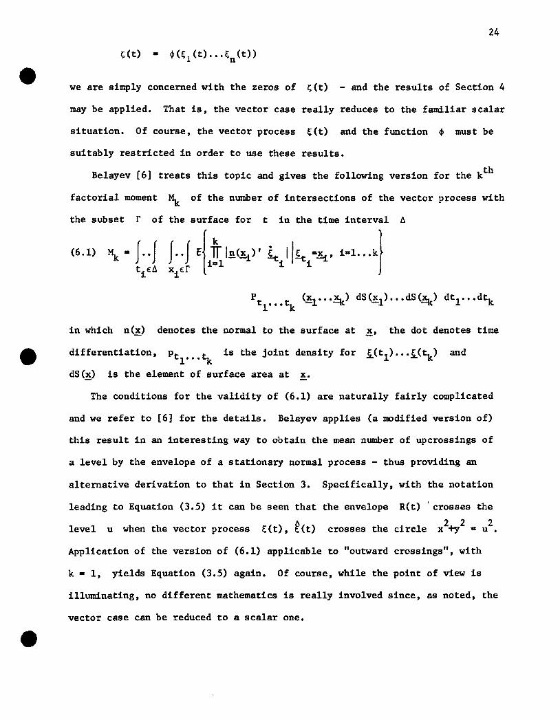
thBelayev [6] treats this topic and gives the following version for the k

factorial moment Mk of the number of intersections of the vector process with

the subset

(6.1)

r of the surface for t in the time interval

f··f E{*l!l(.!.t)' ~ II~ -.!.t, i-I. ..k}r i=l i i

XiE:

in which n(x) denotes the normal to the surface at .!., the dot denotes time

differentiation, Ptl •••~ is the joint density for I(tl) •••I(tk)

dS(~) is the element of surface area at .!..

and

The conditions for the validity of (6.1) are naturally fairly complicated

and we refer to [6] for the details. Belayev applies (a modified version of)

this result in an interesting way to obtain the mean number of upcrossings of

a level by the envelope of a stationary normal process - thus providing an

alternative derivation to that in Section 3. Specifically, with the notation

leading to Equation (3.5) it can be seen that the envelope R(t)' crosses the

level u when the vector process ~(t), ~(t)222

crosses the circle x +y - u •

Application of the version of (6.1) applicable to "outward crossings", with

k • 1, yields Equation (3.5) again. Of course, while the point of view is

illuminating, no different mathematics is really involved since, as noted, the

vector case can be reduced to a scalar one.

25

Crossing problems for (scalar) stochastic processes may also be regarded as

the discussion of the solutions to a random equation ~(t) = 0, ~(t)-u = 0,

etc. We typically ask, "How many solutions are there (for fixed "sample

point" w) to the single equation (i;(t) = 0) in one unknown (t) in some in-

terval, and what are the mean and moments of this number?" As we saw, the case

of a vector process really belongs within this framework.

A more general question is to consider the point process (in nR ) con-

sisting of the solutions to n (random) equation in n unknowns. That is, we

consider a vector stochastic process 5..(.1) = (~l (1.) ••• ~n (1.» where the param­

eter t = (tl ••• t) is also a member of n-dimensional Euclidean space Rn •- n

(We will call such a process a "vector field".) One may, of course, even more

generally let ~ have n components and 1. m-componen~s, and this may lead

to interesting results (e.g. in terms of Hausdorff dimension and measure of the

set of zeros) when n < m. We will not need this extra generality here,

however.

It is not our intention to pursue any general theory for the zeros of

vector-fields, but merely to point out that it is this framework which is

really appropriate for a number of applications. Particularly (in addition to

all the cases considered with n = 1), we would refer to work by Longuet-

Higgins [32] and especially Belayev [7] concerning certain point processes

associated with (ordinary) random fields.

Specifically in [7] Belayev considers a real random field

{~s: s = (sl ••• Sn)ERn}. He deals with three point processes in Rn formed

from such a field, which he terms "bursts", "shines" (alias "flashes", "splashes"

according to translational preferences) and saddle points. A "burst" occurs

at the point s if ~s has a local maximum of height greater than (some

fixed) u at that point. A "shine" occurs at s if ~ > U and the normals

to the ~-surface has a fixed direction - which means that

26

a light ray along this direction would be reflected straight back by the ele-

ment of surface there. A saddle point occurs at s if the normal to the sur-

face there is parallel to the (n+l)-axis and the principal curvatures have

opposite sign.

Thus bursts, shines and saddle points are defined primarily by conditions

on the direction of the normal to the surface - which immediately leads to n

equations to be satisfied in each case. (Of course, in working out, say, the

mean number of "bursts" .!. in a set, we must use the added condition that

~ > u.)s

The point processes of bursts, shines and saddle points are homogeneous

with respect to the group of parallel shifts if the field ~s is homogeneous.

Belayev gives conditions - based on the covariance function for ~s - for these

point processes to have finite intensities. He further obtains explicit

formulae (generalizing (4.1» for the factorial moments of each of the number

of bursts, shines and saddle points in a given set. We refer to [7] for the

details.

7. POISSON APPROXIMA.TIONS FOR LEVEL CROSSINGS

If a stationary point process on the line is "thinned outII by making events

rarer in some way, it is natural to ask whether the remaining events tend (in

some sense) to behave approximately like a Poisson process. Clearly the "less

dependency" there is in the process between distinct time points, the "more

likely" such a result will be. Such questions were investigated first (to our

knowledge) by Volkonski and Rozanov [43] who used strong rrrixing assumptions to

describe the "dependence decay".

One most useful situation in which this has been throughly investigated is

that for the upcorssings of a high level u, by a stationary normal process.

27

As the level increases, the upcrossings become rarer, thus raising the possi-

bi1ity of Poisson-like behaviour. Let us now write N (O,T)u

for the number of

upcrossings of the level u in (O,T) by a stationary normal process ~(t)

(with zero mean, unit variance and covariance function r(T». As u increases,

u ~ 00, in a suitably coordinated

(A2~/2~)eXP(-u2/2), and fixing

Hence we consider a normalized version

lJ == EN (0,1) ..u

Specifically, writing

N (O,T) will tend to become smaller.u

of N (O,T) formed by letting T ~ 00 asu

way.

T > 0 we wish to have

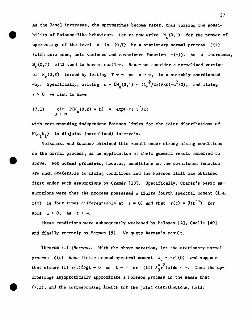
(7.1)

with corresponding independent Poisson limits for the joint distributions of

N(aibi ) in disjoint (normalized) intervals.

Vo1konski and Rozanov obtained this result under strong mixing conditions

on the normal process, as an application of their general result referred to

above. For normal processes, however, conditions on the covariance function

are much preferable to mixing conditions and the Poisson limit was obtained

first under such assumptions by Cramer [13]. Specifically, Cramer's basic as-

sumptions were that the process possessed a finite fourth spectral moment (i.e.

is four times differentiable at T == 0) and that -ar(t) == O(t ) for

some a > 0, as t ~ 00.

These conditions were subsequently weakened by Be1ayev [4], Qualls [40]

and finally recently by Berman [9]. We quote Berman's result.

Theorem 7.1 (Berman). With the above notation, let the stationary normal

process ~(t) have finite second spectral moment A == -r"(O) and suppose2

00 2that either (i) r(t)!ogt ~ 0 as t ~ 00 or (ii) fOr (s)ds < 00. Then the up-

crossings asymptotically approximate a Poisson process in the sense that

(7.1), and the corresponding limits for the joint distributions, hold.

28

In fact Berman proves more than this. He shows that the upcrossings of a

high level and downcrossings of a low level are independently distributed in

Poisson fashion asymptotically as the levels tend to ±oo.

An important use for Theorem 7.1 concerns the evaluation of the asymptotic

distribution for the maximum M(T) of the stationary normal process ~(t) in

° ~ t S T. This connection is easily seen since

Pr{N (O,T) ... O} = Pr{~(O»u, N (O,T)=O} + Pr{M(T) ~ u}.u u

The first term on the

right is dominated by Pr{~(O»u} which tends to zero as u ~ 00. Hence

Pr{M(T)Su} can be approximated by Pr{N (O,T)==O}u

as u, T ~ 00 in a coordinated

manner. This leads in fact to

as T ~ 00 (cf. [14], Section 12.3).

-zexp(-e )

Other topics related to the Poisson nature of the upcrossings of a high

level include the distribution of the total time spent above a high level in an

interval and of the length of a single excursion above a high level. This

latter quantity is again the distribution of time from an "arbitrary" up-

crossing to the next downcrossing for which the series expression holds. How-

ever, if the level is very high, it may be shown that such an excursion - suit­

2ably scaled - has an asymptotic distribution with density ~TItexp(-(TI/4)t).

A discussion of the history of results of this kind appears in [14, Section

12.4, 12.5]. More recent work appears in [8] and closely related work in [10].

The basic assumption made in considering the Poisson nature of the up-

crossings of a very high level was that the stationary normal process ~(t)

had a finite second spectral moment If A "" 002 '

then the mean number of

upcrossings of any level u is infinite and indeed there may be positive

29

probability that the number of upcrossings itself is infinite. This of course

does not provide a point process with any of the usual properties of good be-

haviour. However, some interesting properties may still be obtained under

useful assumptions, in particular when the covariance function r(.) satisfies

(7.2) as It I -+ 0

where C is a finite non-zero constant and 0 < a < 2. The case a = 2 is

that previously considered (A2 < =). The case a = I includes the

Ornstein-Uhlenbeck process with r(T). exp(-al.I).

It has been shown by S. Orey [36] that when r(T) satisfies (7.2) (and

certain other assumptions) then the set of crossings has Hausdorff dimension

aI - 2. Thus even though infinitely many crossing events occur in finite in-

tervals, their "density" may be described via their Hausdorff dimension.

There is, of course, no hope of obtaining a Poisson result for upcrossings

of a high level. However, a device of Pickands [37] for "thinning" the up-

crossings to get a well-behaved point process does allow a Poisson result to

be derived, and this result is useful in discussing extreme value distributions

for such processes.

To be precise, Pickands discusses "c:-upcrossings" which are defined for

€ > 0 to be those upcrossing points t for which (t-€,t) contains no other

upcrossing. The number of c:-upcrossings of a level u in any finite interval

is finite - indeed a bounded random variable since it cannot exceed (length

of interval)/€. Pickands shows in [37] that if, in addition to (7.2), either

r(t)l.ogt -+ 0 as = 2t -+ = or fOr (t)dt < =, then as asymptotic Poisson prop-

erty holds for the €-upcrossings. This result may again be used to obtain the

asymptotic distribution of the maximum ([38]).

30

Finally, we note that other forms of limiting result are possible (for, say,

the zeros of a stationary normal process with AZ < =). In the case considered

the crossings were made rare and hence approximately Poisson by letting the

level u ~ =. For a fixed level, it may be shown under certain conditions that

the number of zeros (suitably normalized) has an asymptotic normal

distribution (cf. [34]), in long time intervals.

8a loCAl... EXTREfvES

In this final section, we shall briefly consider some aspects of the

occurrence of local extremes of a stationary normal process ~(t) (again with

zero mean, unit variance and covariance function r(T».

A local maximum or minimum may be defined in terms of "continuity prop-

erties" of the sample path (e.g. a local maximum may be said to occur at to

if ~(t) < ~(tO) for all t in some neighbourhood of to)' However, there is

little point in so doing, since the conditions one wishes to assume will virtu-

ally always imply the existence of a continuous sample derivative. This being

so, the local maxima (minima) of ~(t) are simply the downcrossings (up­

crossings) of zero by F;'(t). Since ~'(t) has covariance function -r"(T),

it follows that the mean number of local maxima and minima per unit time are

finite if and only if A4

• _r(4)(0) < = and are each given by

(1/2n)(A4/Az)~' These and other properties of the local extremes are developed

in [27]. (See also [17] for a development via "continuity properties".)

A problem of some interest - which has recently been studied in considerable

detail by G. Lindgren - concerns the behaviour of a stationary normal process

~(t) in the neighbourhood of a local maximum. In particular, what Lindgren

calls the "wavelength" (time or lIcres t-trough time" to the next minimum) and

31

the "wave-height" (drop in height from the maximum to the minimum or "crest­

trough height") have had some attention in the past (cf. [12]).

In [29], Lindgren shows that given a local maximum of height u at t· 0,

~(t) has the same finite dimensional distributions as a process uA(t) +

61(t) - 62 (t) where A(t) is a certain deterministic function, 6

1is a non­

stationary zero mean normal process with a certain covariance function, and

62 is an independent deterministic process of the form ~B(t) where ~ is a

random variable and B a known function. (The condition "given an event at

t-O" must be appropriately interpreted, of course - cf. [29] for the details

of this and the specific functional forms of A, B and the distribution of

~.) This representation is, incidentally, motivated by one of Slepian in a

different context.

Lindgren studies the behaviour of ~(t) in the neighbourhood of a very low

maximum ([29]) and uses the results in [30] to obtain the limiting distribution

of the wavelength and wave-height as u ~ -00. Similar questions are studied

in [31] for the (perhaps most interesting) case when u ~ +00.

32

REFERENCES

[1] Bartlett, M.S. An Introduction to Stochastic Processes,Cambridge University Press, 1956.

[2] Be1ayev, Yu.K. "Continuity and H61der's conditions for sample functionsof stationary Gaussian processes" FPoc. 4th Berk. Symp. on Math.Stat. and Probability 2 (1961) p. 23-33.

[3] "On the number of intersections of a level by a Gaussian sto-chastic process" Teor. Ver. i. PM-me 11 (1966) p. 120-128.

[4] "On the number of intersections of a level by a Gaussian sto-chastic process II" Teor. Ver. i. Mm. 12 (1967) p. 444-457.

[5] "Elements of the general theory of random streams" Appendix toRussian edition of Stationazry and Related Stochastic Processesby H. Cram~r and M.R. Leadbetter, HIR Moscow 1969 (English transla­tion in University of N. Carolina Mimeo Series No. 703).

[6] "On the number of exits across a boundary of a region by a vec-tor stochastic process" Teor. Ver. i. PM-me 13 (1968) p. 333-337.

[7] "Bursts and shines of random fields" Doklady Akad. Nauk SSSR176 (1967) p. 495-497.

[8] Be1ayev, Yu.K. and Nosko, V.P. "Characteristics of excursions above ahigh level for a Gaussian stochastic process and its envelope"Teor. Ver. i. PM-me 14 (1969) p. 302-314.

[9] Berman, S.M. "Asymptotic independence of the numbers of high and lowlevel crossings of a stationary Gaussian process" Annals Math.Statist. June 1971.

[10] "Excursions above high levels for stationary Gaussian processes"To appear Pacific~. Math.

[11] Bulinskaya, E.V. "On the mean number of crossings of a level by astationary Gaussian process" Teor. Ver. i. PM-me 6 (1961)p. 474-477.

[12] Cartwright, D.E. and Longuet-Higgins, M.S. "The statistical distributionof the maxima of a random function" Proc. Roy. Soc. A 237 (1956)p. 212-232.

[13] Cram~r, H. "On the intersections between the trajectories of a normalstationary process and a high level" Ark. Mat. 6 (1966) p. 337­349.

[14] Cram~r, H. and Leadbetter, M.R. Stationazry and Related StochasticProcesses Wiley, New York, 1967.

[15] Cram~r, H., Leadbetter, M. R. and Serfl1ng, R.J. "On distribution func­tion - moment relationships in a stationary point process" Z. Wah!'.ve~. Geb. 18 (1971) p. 1-8.

33

[16} Fieger, W. '~e number of y-1evel crossing points of a stochasticprocess" Z. Wahr. ver. Geb. 18 (1971) p. 227-260.

[17} "The number of local maxima of a stationary normal process"Math. Soand. 25 (1969 p. 218-226.

[18] Ito, K. "The expected number of zeros of continuous stationaryGaussian processes" J. Math. Kyoto Univ. 3-2 (1964) p. 207-216.

[19] Ivanov, V.A. liOn the average number of crossings of a level by samplefunctions of a stochastic process" Teor. Ver. i. Prim. 5 (1960)p. 319-323.

[20] Kac, M. "On the average number of real roots of a random algebraicequation" BuZ.Z. Amer. Math. Soo. 49 (1943) p. 314-320.

[21J Leadbetter, M.R. "On crossing of arbitrary curves by certain Gaussianprocesses" PPOo. Amer. Math. Soo. 16 (1965) p. 60-68.

[22J "On crossings of levels and curves by a wide class of stochasticprocesses" AnnaZs. Math. Statist. 37 (1966) p. 260-267.

[23] "A note on the moments of the number of axis crossings by a sto-chastic process" Bul'L. Amer. Math. Soo. 73 (1967) p. 129-132.

[24] "On streams of events and mixtures of streams" J. Roy. Stat.Soo. (B) 28 (1966) p. 218-227.

[25J "On the distributions of the times between events in a stationarystream of events" J. Roy. Stat. Soc. (B) 31 (1969) p. 295-302.

[26] "On certain results for stationary point processes and theirapplication" Bul'L. I.S.I. 43 (1969) p. 309-320.

[27] "Local maxima of stationary processes"Proc. Camb. PhiZ. Soc. 62 (1966) p. 263-268.

[28] "On basic results of point process theory" To appearProc. 6 Berk. Symp. on Math. stat. and Probability.

[29] Lindgren, G. "Some properties of a normal process near a local maxi­mum" Annals Math. Stat. 41 (1970) p. 1870-1883.

[30J "Extreme values of stationary normal processes"z. Wahr. ve~. Geb. 17 (1971) p. 39-47.

[31J "Wavelength and amplitude for a stationary process after a highmaximum-decreasing covariance function" University of NorthCarolina Institute of Statistics Mimeo Series No. 746.

[32] Longuet-Higgins, M.S. "The statistical geometry of random surfaces"Hydrodynamic Instability, Proo. Symp. AppZ. Math. 13" Amer. Math.Soo. (1962) p. 105-143.

34

[33] "The distribution of intervals between zeros of a stationaryrandom function" Phit. Trans. Roy. Soo. 254 (1962) p. 557-599.

[34] Ma1evich, T.L. "Asymptotic normality of the number of crossings oflevel zero by a Gaussian process" Teor. Ver. i. Pl'im. 14(1969) p. 287-309.

[35] Matthes, K. "Stationilre Zufl1lige Punktfo1gen I"Janr. d. DMV 66 (1963) p. 66-79.

[36] Orey, S. "Gaussian sample functions and the Hausdorff dimension oflevel crossings" Z. Wahr. venue Geb. 15 (1970) p. 249-256.

[37] Pickands, J. "Upcrossing probabilities for stationary Gaussian processes"Trans. Amer. Math. Soo. 145 (1969) p. 51-73.

[38] "Asymptotic properties of the maximum in a stationary Gaussianprocess" Trans. Amer. Math. Soo. 145 (1969) p. 75-86.

[39] Piterbarg, V.I. "The existence of moments for the number of levelcrossings by a stationary Gaussian process" Doktai1y Akad. Nauk.SSSR 182 (1968) p. 46-48.

[40] Qualls, C. "On a limit distribution of high level crossings of astationary Gaussian process" Annats Math. Stat. 39 (1968)p. 2108-2113.

[41] Rice, 5.0. ''Mathematical analysis of random noise"Bett Syst. Tech. J. 24 (1945) p. 46-156.

[42] Y1visaker, N. D. "The expected number of zeros of a stationary Gaussianprocess" Annats Math. Stat. 36 (1965) p. 1043-1046.

[43] Vo1konski, V.A. and Rozanov, Yu.A. "Some limit theorems for randomfunctions I and II" Teor. Ver. i. Pl'im. 4 (1959) p. 186-207and 6 (1961) p. 202-215.