M A X P L A N C K S O C I E T Y

Preprints of theMax Planck Institute for

Research on Collective GoodsBonn 2011/13

Procrastination in Teams, Contract Design and Discrimination

Philipp Weinscheink

Preprints of the Max Planck Institute for Research on Collective Goods Bonn 2011/13

Procrastination in Teams, Contract Design and Discrimination

Philipp Weinschenk

July 2011

Max Planck Institute for Research on Collective Goods, Kurt-Schumacher-Str. 10, D-53113 Bonn http://www.coll.mpg.de

PROCRASTINATION IN TEAMS,

CONTRACT DESIGN, AND DISCRIMINATION

Philipp Weinschenk∗

May 2011

Abstract

We study a dynamic model of team production with moral hazard. We show

that the players begin to invest effort only shortly before the time limit when

the reward for solving the task is shared equally. We explore how the team

can design contracts to mitigate this form of procrastination and show that

the second-best optimal contract is discriminatory. We investigate how limited

liability or the threat of sabotage influences the team’s problem. It is further

shown that players who earn higher wages can be worse off than teammates with

lower wages and that present-biased preferences can mitigate procrastination.

JEL Classification: D82, L22, J71, M52.

Keywords: moral hazard, team production, partnerships, procrastination, con-

tract design, discrimination.

1 INTRODUCTION

Team production is widely used in organizations (Katzenbach and Smith 1993) and

it has become increasingly important over the last decades (Wuchty, Jones, and Uzzi

2007). A common problem of team production is that individual contributions cannot

be identified, which causes moral hazard (Holmstrom 1982, Prendergast 1999).

∗Max Planck Institute for Research on Collective Goods, Kurt-Schumacher-Str. 10, 53113 Bonn,

Germany, weinschenk@coll.mpg.de, and Bonn Graduate School of Economics. I thank Philippe

Aghion, Oliver Hart, Martin Hellwig, Marco Kleine, and Christian Traxler, as well as seminar

participants at Harvard University and the Max Planck Institute in Bonn for helpful comments and

suggestions. Part of the research was carried out while I visited Harvard University. I thank Harvard

University for their hospitality during my visit there.

2

This paper contributes to the understanding of the dynamic aspects of moral

hazard in teams. We examine how the externalities from team production induce

not only static, but also rich dynamic effects. We consider a simple model where a

team, consisting of perfectly rational and time-consistent players, works on a joint

task, which yields a reward when solved.1

Our first result is that when the reward is shared equally among players and

the time limit for solving the task is sufficiently long, the team procrastinates in the

sense that members invest effort only shortly before the time limit. Consider a simple

example with two players, who have two periods to solve a task. The task is solved in

a period with probabilities 1/2, 1/4, or 0 when respectively both, one, or no player(s)

invest(s) effort in this period. Effort causes private costs of 1. Solving the task yields

a per-capita reward of 5. In period 2, a player’s additional expected payoff from

investing is 1/4 × 5 − 1 > 0. Hence, both players invest effort, conditional that the

task is not yet solved. The expected payoff from period 2 is 1/2×5−1 = 3/2 when the

task is not yet solved and zero otherwise. In period 1, a player’s additional expected

payoff from investing is 1/4 × (5 − 3/2) − 1 < 0. Thus, players do not invest in

period 1. The key intuition is that team production in the future causes externalities

which make investing effort in the present less worthwhile. Procrastination is socially

inefficient, but individually rational.2

As a benchmark case, we consider the game with a single player. Because the

externalities from team production are absent the player does not procrastinate.

Consider the example from before. The player invests in period 2 (conditional that

the task is not yet solved) because the additional expected payoff from investing is

1/4×5−1 > 0. The expected payoff from period 2 is 1/4×5−1 = 1/4 when the task

is not yet solved. The player also invests in period 1 because the additional expected

payoff from investing is 1/4× (5− 1/4)− 1 > 0.

Motivated by the finding that a team may procrastinate when players are remu-

1See Cohen and Bailey (1997) for examples how organizations use so called project teams, which

are usually time-limited and non-repetitive (p. 242).2O’Donoghue and Rabin (1999) define procrastination as “wait when you should do it” (p. 104).

In the example, if both players invest also in period 1, the team’s expected payoff is 1/2× 10− 2 +

1/2× 3 = 9/2 instead of just 2× 3/2 = 3 when players procrastinate.

3

nerated equally, we explore how the team can design a wage contract that mitigates

procrastination. Our investigation primarily concerns two questions: which effort

profile is implemented, and what contract leads to its implementation? While effort

is noncontractible, we allow the team to condition each player’s wage in each period

on whether the task is solved or not. We require that the team’s budget is balanced,

which can be understood as a consequence of feasibility and renegotiation-proofness.

We show that when the first-best (where all players invest, as long as the task is not

solved) is implementable, one can implement it with the equal-sharing contract, where

all players receive the same share of the team’s reward. When the time limit is suffi-

ciently long, we know from before that players procrastinate with the equal-sharing

contract. In this case the first-best is not implementable.

We then investigate the properties of second-best contracts. We first show that

the equal-sharing contract is not second-best. The idea is that by discriminating

between players (in the sense of remunerating them differently) one can induce a

player, or some players, to invest effort in an early period, at a time when under the

equal-sharing contract no player would invest. As a general result, we show that a

second-best contract has to be discriminatory. To see that discriminatory contracts

mitigate procrastination in teams, consider again the previous example. Suppose that

when the task is solved in period 1, player 1 receives the team’s reward of 10, while

player 2 receives nothing. When the task is solved in period 2 each player still receives

5. Then player 1 invests effort in period 1 because her additional expected payoff

from investing is 1/4× (10− 3/2)− 1 > 0. Player 2 does not invest in period 1 and

(when the task is not solved) both players invest in period 2. By the aforementioned

change of the first-period rewards, the team’s expected payoff improves from 3 to

1/4× 10− 1 + 3/4× 3 = 15/4.

We specify a wage contract, called “handsome contract”, which induces all players

except one to invest in early periods (i.e., periods where the team does not invest

with the equal-sharing contract) and all players to invest in late periods. We show

that the handsome contract is second-best and renegotiation-proof. There may also

exist other contracts which are second-best. But when we require the contract to be

renegotiation-proof, all contracts which are second-best implement the same effort

profile (i.e., the same number of players to invest in each period) as the handsome

4

contract. We then explore how limited liability or the threat of sabotage restricts

the team’s contract design problem. We show that both issues can seriously limit the

team’s possibilities to mitigate procrastination, especially when there are more than

two players.

Since our model is easily tractable, we can gain several additional insights. First,

when we allow the team to hire a principal the first-best can be implemented when

the team members are fully liable. When the team members are protected by limited

liability and the time limit is sufficiently long, this is no longer true. The idea is that

with a long time limit the wages in early periods have to be huge to convince the

team members to invest effort. The principal would then earn a negative expected

profit, which makes implementing the first-best impossible.

Second, discriminatory wage contracts often lead to differences in players’ well-

being. Interestingly, players who earn higher wages can be worse off than teammates

with lower wages. The reason is that players with higher wages may be motivated to

invest effort, but teammates with lower wages may not be motivated. Due to team

production, the latter benefit from the formers’ investments, while they do not have

to bear effort costs. This effect can overcompensate the wage differences. The finding

has the severe implication that an outside party (e.g., a judge) is in general not able

to infer that player A is disadvantaged compared to B when A receives lower wages

than B.

Third, the model we consider can also be interpreted as a public-good game.

Numerous experiments show that in such games people contribute more than they

should if they were selfish, which indicates that people are often not purely selfish.3

In an extension of our model, we suppose that players have social preferences, in the

sense that they take other players’ well-being (at least partly) into account. We first

show that players begin to invest effort earlier than when they are selfish. That is,

procrastination is alleviated by social preferences. Unless players are fully altruistic,

however, the players still procrastinate when rewarded equally and the time limit is

sufficiently long. We further consider the case where players differ with respect to their

social preferences. For this case it is better to have heterogenous teams (where players

3For stronger evidence, see, for example, Andreoni (1995).

5

have different social preferences) than having homogenous teams (where players have

the same social preferences).4

Fourth, present-bias preferences can mitigate procrastination. The idea is that

present-biased players put less weight on the future externalities arising from team

production. This insight is highly interesting because many models explain procras-

tination by means of present-bias preferences (e.g., Akerlof 1991, Laibson 1997, and

O’Donoghue and Rabin 1999, 2001).

Related Literature.— Our paper is related to the huge literature on moral haz-

ard in teams, which is pioneered by Alchian and Demsetz (1972) and Holmstrom

(1982).5 Most of this literature either considers static models or dynamic models

with a repetition of a one-period game. A remarkable exception is Bonatti and

Horner (forthcoming). Independently of our work, they developed a model where

teams procrastinate. They put a strong emphasize on the effects of uncertainty and

learning (they assume that players do not know the production technology) and show

that observability of effort highly influences their results. In our model the produc-

tion technology is known6 which has the consequence that it is not important whether

effort is observable or not. Their main interest is the infinity horizon case, where they

characterize the Markov perfect equilibrium when effort costs are linear. We briefly

study the infinite horizon case and are able to characterize the Markov perfect equi-

librium for our model also for the case when effort costs are nonlinear. An interesting

result of our analysis is that a team may benefit from a lower discount factor. Our

main focus, however, is the case with a finite horizon, where we study in depth the

question how contracts are optimally designed. Contract design is not the focus of

Bonatti and Horner. They briefly study mechanisms for the infinite horizon case and

assume that wages have to be nondiscriminatory.7 As our analysis reveals, discrim-

4Interestingly, Hamilton, Nickerson, and Owan (2003) show empirically that teams which are

more heterogenous with respect to the abilities of their members are more productive.5We especially contribute to the branch of the literature on moral hazard in teams which explores

optimal sharing rules for teams when there is no principal and the team’s budget has to be balanced;

see Holmstrom (1982), Radner (1986), Radner, Myerson, and Maskin (1986), Rasmusen (1987),

Legros and Matthews (1993), and Strausz (1999).6This is in line with most agency models in the literature.7Another difference is that they require that the team’s budget has to be balanced only on average

6

inatory contracts are key instruments to alleviate procrastination. We also study

how renegotiation-proofness, limited liability, or the threat of sabotage influences the

team’s design problem. Bonatti and Horner put a strong emphasize on deadlines.

We show that in our model designing a discriminating contract is a better measure

to mitigate procrastination than a deadline, at least when the discount factor is suf-

ficiently close to one.8 Because our model allows for a very simple characterization

of the solution, we are able to extend our baseline model in several interesting ways.

Next to the extensive study how contracts are optimally designed, we explore issues

like present-biased preferences and social preferences and team design.

We also contribute to the economic literature on discrimination, which started

with Becker (1957). He argues that market forces are effective means to repress

discrimination because firms which discriminate are less efficient than those who

do not. A problem with this argument is, however, that it cannot explain why

discrimination persists (Stiglitz 1973, Arrow 1998). In our model discrimination is

necessary to mitigate procrastination in teams and mandatory when implementing

the second-best. Winter (2004) provides a static model of team production with moral

hazard and an increasing returns to scale production technology. His main result is

that when one requires the Nash equilibrium to be unique, the optimal contract is

discriminatory. For surveys, see Darity and Mason (1998) and Holzer and Neumark

(2000, 2006).

The paper proceeds as follows. In Section 2, we present the basic model, which is

then analyzed in Section 3. In Section 4, we explore how the team can design a wage

contract that mitigates procrastination and study how constraints like renegotiation-

proofness, limited liability, and the threat of sabotage influences the team’s problem.

We also investigate the case where the team can hire a principal. In Section 5, we

offer some extensions. We conclude in Section 6. Proofs are relegated to Appendix

A.

(which requires a third party).8Moreover, a problem of deadlines is that they are not renegotiation-proof: players prefer to

ignore a deadline once it is reached.

7

2 THE MODEL

A set of risk-neutral and time-consistent players N := {1, ..., n} works on a joint task.

Time is discrete and indexed by t ∈ {1, 2, ...}. The team has T ≥ 2 periods of time

to solve the task. The time limit T is potentially very large, but finite.9 It can be

interpreted as the time when solving the task is no longer economically interesting;

see Section 5.4.

When the task is solved the team obtains a joint reward of Z > 0, which is

immediately paid. Initially we assume that the reward is shared equally so that each

player receives z := Z/n.10 When the task is not solved in period t, then each player

receives 0 in t.

At the beginning of period t, each player i decides how much effort to invest:

et,i ∈ {0, 1}, where 0 denotes no effort and 1 effort.11 Effort costs are private and

normalized to et,i. It is useful to define et :=∑

N et,i as the team’s investment in

effort in period t. The vector e = (e1, ..., et, ..., eT ) is denoted as the effort profile.

The probability that the task is solved in t is p × et, where 0 < p < 1/n.12 The

idea is that when more players invest effort in a period, it is more likely that the

task is solved in this period. The effort decisions made by players are not verifiable

and therefore not contractible. Because the production technology is known and our

arguments rely on backward induction, it is not important whether effort is observable

or not by other players.

When the task is solved at the end of period t or we are at the end of period

T , the game ends. Otherwise, the next period begins and players decide again how

much effort they want to invest. We start with the simplest case where there is no

discounting.13

Player i’s strategy is the plan which describes how much effort she invests in

9In Section 5.2, we explore the case when there is no time limit for solving the task.10In Section 4, we investigate how the team optimally shares the reward.11Alternatively, each player chooses effort from the continuum [0, 1]. When marginal effort costs

are constant, this does not change our analysis.12In Section 5.3, we examine more general success functions.13We consider discounting in Section 3.3.

8

which period, conditional that this period is reached.14 Formally, i’s strategy is

si = (e1,i, ..., et,i, ..., eT,i). The solution concept we use is subgame perfect Nash

equilibrium.

3 ANALYSIS

Denote player i’s continuation payoff of reaching period t by Ct,i. The continuation

payoff can also be interpreted as the expected payoff of the player, from t to T . It

depends on the parameters of the game (p, z, n, T ) as well as on the players’ strategies.

Because the game ends, at the latest, after period T , we have Ct,i = 0 ∀t > T, i ∈ N .

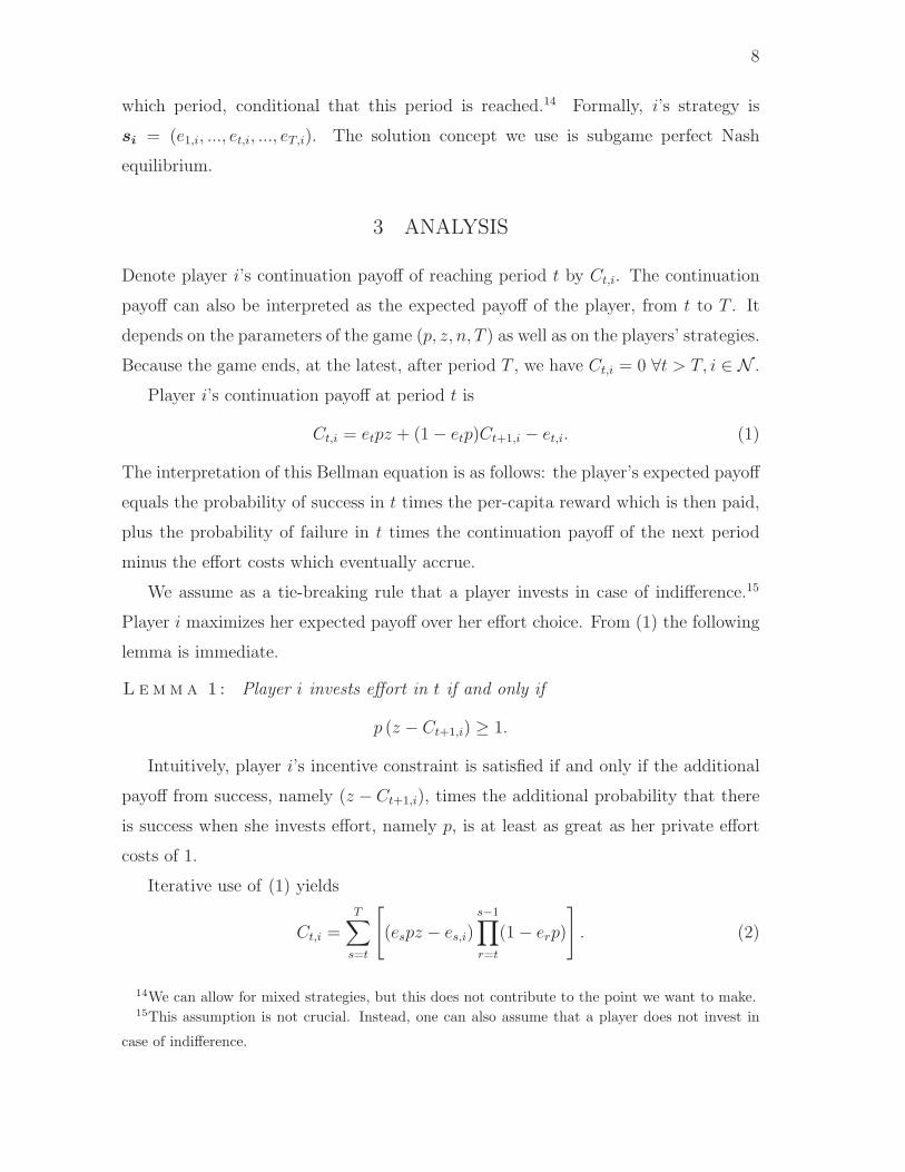
Player i’s continuation payoff at period t is

Ct,i = etpz + (1− etp)Ct+1,i − et,i. (1)

The interpretation of this Bellman equation is as follows: the player’s expected payoff

equals the probability of success in t times the per-capita reward which is then paid,

plus the probability of failure in t times the continuation payoff of the next period

minus the effort costs which eventually accrue.

We assume as a tie-breaking rule that a player invests in case of indifference.15

Player i maximizes her expected payoff over her effort choice. From (1) the following

lemma is immediate.

L e m m a 1: Player i invests effort in t if and only if

p (z − Ct+1,i) ≥ 1.

Intuitively, player i’s incentive constraint is satisfied if and only if the additional

payoff from success, namely (z − Ct+1,i), times the additional probability that there

is success when she invests effort, namely p, is at least as great as her private effort

costs of 1.

Iterative use of (1) yields

Ct,i =T∑

s=t

[

(espz − es,i)s−1∏

r=t

(1− erp)

]

. (2)

14We can allow for mixed strategies, but this does not contribute to the point we want to make.15This assumption is not crucial. Instead, one can also assume that a player does not invest in

case of indifference.

9

Because a player cannot obtain z for sure and effort costs are nonnegative, Ct,i < z

for all t ∈ {1, ..., T}, i ∈ N . From (1) we see that this implies that a player always

benefits when another player invests effort.

It is useful to denote the continuation payoff of reaching period t, given that

all players always invest from t until T , as Ct,i. Throughout the paper we mean

by investing in some future period, investing conditional that this period is reached

because the task is not yet solved. From (2) we get that

Ct,i = (npz − 1)1− (1− np)T−t+1

np. (3)

Because a player can always decide not to invest, a continuation payoff is never

negative. Together with Lemma 1, this implies that a necessary condition for invest-

ment is the following.

A s s u m p t i o n 1 : pz ≥ 1.

Throughout the paper we maintain Assumption 1. We briefly discuss it in Section

4.6.3. Assumption 1 implies that in the static game (T = 1) all players invest effort.

We first look at the benchmark case, where the social planner solves the problem.

P r o p o s i t i o n 1 : For the special case where n = 1 and pZ = 1 welfare is zero

for all investment profiles. Otherwise, in the first-best all players always invest effort.

Moreover,∑

N Ct,i increases with a higher level of effort es, where s ≥ t.

Intuitively, welfare is maximized when players use every chance to solve the task,

i.e., always invest effort when the task is not solved.

3.1 SINGLE PLAYER

Suppose there is a single player. Because CT+1,1 = 0, Lemma 1 implies that the

player invests in T if and only if pz ≥ 1, which holds because of Assumption 1.

To determine the player’s decisions in the other periods we have to determine

whether or not the following inequality holds for all t ∈ {1, ..., T}

p(

z − Ct,1

) ?

≥ 1. (4)

10

For the limit case we yield, using (3),

p(

z − limT→∞

Ct,1

)

= 1. (5)

Note that Ct,1 is increasing in T . Therefore, for any finite T we have

p(

z − Ct,1

)

≥ 1. (6)

From before, we already know that the player will invest in T . Given this, CT,1 = CT,1.

Therefore, Lemma 1 and (6) imply that it is optimal for the player to invest in T −1.

Then CT−1,1 = CT−1,1 and it is again optimal for the player to invest in T − 2. These

arguments can be repeated and imply the following proposition.

P r o p o s i t i o n 2 : A single player always invests effort.

The intuition is that the player always invests, because there are no externalities

from team production and so her continuation payoff is rather small in early periods

also.

3.2 SEVERAL PLAYERS

Consider now the case with n ≥ 2 players. From Lemma 1 we see that players invest

in T because CT+1,i = 0. Similar to the case with a single player, we are interested

in whether or not the following inequality holds:

p(

z − Ct,i

) ?

≥ 1. (7)

In the limit case we have, using (3),

p(

z − limT→∞

Ct,i

)

= p

(

z − (npz − 1)1

np

)

=1

n< 1. (8)

Therefore, when the time limit is sufficiently long it cannot hold that players always

invest effort.

We want to explore exactly when players invest effort and when not. The following

lemma is useful.

L e m m a 2: (i) Players choose the same investment in period t. This holds for all

t ∈ {1, ..., T}.

11

(ii) When players invest no effort in t then Ct,i = Ct+1,i.

(iii) When players invest effort in t then Ct,i > Ct+1,i.

(iv) Ct,i = Ct,i when players always invest from t on and Ct,i < Ct,i, otherwise.

The intuition for part (i) is that players are symmetric and therefore always choose

the same investment. That is, either all players invest effort or not in a specific period.

The reason why part (ii) holds is that when nothing happens in period t, then the

expected payoff at the beginning of period t is the same as at the beginning of period

t + 1. Because investing effort by all agents is beneficial, in the sense that all are

better off, part (iii) holds. The intuition for part (iv) is that when players invest less

than in the first-best, their expected payoffs suffer.

P r o p o s i t i o n 3 : (i) When the time limit is sufficiently short, namely T ≤

x+ 1, where

x =ln(n− 1)− ln(npz − 1)

ln(1− np),

then players always invest effort.

(ii) When the time limit is sufficiently long, namely T > x + 1, then players do

not invest effort in periods t < T − x and invest effort in the periods t ≥ T − x.

So when the time limit is long, players will invest if and only if there are sufficiently

few periods left. This is in stark contrast to the findings with a single player, who

always invests effort. Intuitively, when there is team production, each player knows

that shortly before the time limit all players will invest effort. Then team production

generates externalities. Therefore, not investing is very attractive in early periods,

because this allows the player to exploit the future externalities arising from team

production. Technically, due to the externalities of team production the continuation

payoffs are too large to always sustain investment in effort.

Note that Proposition 1 implies that all players would be better off if all invest

at all times. Because players’ inactivity is collectively harmful to them, we also

call inactivity procrastination. Proposition 3 can be rephrased as follows: when the

time limit is sufficiently long, the team procrastinates. Procrastination is socially

inefficient, but individually rational because in the early periods of a game, a player

is individually better off when she does not invest.

12

Note that the reason why it is optimal for a player not to invest in the early

periods is not that the player hopes that some other player will invest effort and

eventually solve the task. Each player is fully aware that the other players will, like

her, not invest effort in early periods.

We are interested in the comparative statics.

P r o p o s i t i o n 4 : dx/dz > 0. Fixing z, dx/dn < 0. Fixing Z, dx/dn < 0.

In words, with a higher per-capita reward z procrastination is less likely16 and

players begin to invest earlier. Intuitively, the advantage of not investing today is that

future externalities arising from team production can be exploited. The drawback is

that it is less likely that the reward is ever received. With a higher per-capita reward

the latter aspect becomes more important.

The intuition why procrastination is more likely and players begin to invest later

when the number of players increases is that then the aforementioned externalities

from team production become more important. Technically, the continuation payoff

when all players invest is increasing in the size of the team. The effect of a higher

success parameter p on x is ambiguous.

One can yield the following result regarding the likelihood that the task is ever

solved.

P r o p o s i t i o n 5 : A single player is more likely to solve the task than n ≥ 2

players if T is sufficiently large. It is the other way round when T is sufficiently

small.

The intuition is simple. Because a single player always invests, the likelihood that

she solves the task sometimes approaches 1 when the time limit is very long. With

several players this is not true, because they invest only in the last few periods.

3.3 DISCOUNTING

In this section, we explore how players invest when they discount future payoffs. We

first consider the case where players are exponential discounters. Then we study

16Less likely in the sense that it occurs for a smaller parameter set.

13

the case where players are time inconsistent and their intertemporal preferences are

described by quasi-hyperbolic discounting.

3.3.1 EXPONENTIAL DISCOUNTING

Suppose that players are time consistent and use a per-period discount factor of

δ ∈ (0, 1]. As in the case without discounting a social planner directs players to

always invest effort.

P r o p o s i t i o n 6 : In the first-best players always invest effort.

In period t, player i’s expected utility is

Ut,i = Et

[T∑

s=t

δs−tus,i

]

, (9)

where δ ∈ (0, 1] and us,i is the instantaneous utility experienced in period s.

The Bellman equation (1) gets

Ct,i = etpz + (1− etp)δCt+1,i − et,i. (10)

Iteratively using it yields

Ct,i =T∑

s=t

[

(espz − es,i) δs−t

s−1∏

r=t

(1− erp)

]

(11)

and

Ct,i = (npz − 1)1− (δ(1− np))T−t+1

1− δ(1− np). (12)

From (10), it is optimal for player i to invest in period t if and only if

p(z − δCt+1,i) ≥ 1. (13)

The next proposition says that discounting weakly improves the players incentives to

invest.

P r o p o s i t i o n 7 : With discounting players invest in all periods where they

would also invest without discounting and they may invest in more periods.

14

The intuition is that discounting lowers the present value of reaching future pe-

riods. Thereby investing effort in the present gets more attractive. Proposition 7

implies together with Proposition 2 that a single player always invests effort also

when there is discounting.

Another result, see the next proposition, is that for low discount factors δ there

is no procrastination. The intuition is that for low discount factors players care little

about the future externalities arising from team production.

P r o p o s i t i o n 8 : When δ ≤ δ := (pz−1)(pz−1)+p(n−1)

then players always invest ef-

fort. When δ > δ and T is sufficiently large, players do not always invest effort.

The following result says that with discount factors close to 1 nothing changes

compared to the case without discounting.

P r o p o s i t i o n 9 : Generically, for every game (p, z, n, T ) there exists a δ < 1

such that for all δ ∈ (δ, 1) the equilibrium is the same as without discounting (δ = 1).

When the periods (or even the time limit) are short it is reasonable to assume

that the discount factor is close to 1. Then discounting does, at least qualitatively,

not change much, cf. Propositions 8 and 9.

3.3.2 QUASI-HYPERBOLIC DISCOUNTING

We next consider the case where players are time-inconsistent and present-biased.

Formally, we assume that players have β − δ preferences, see Phelps and Pollak

(1968) and Laibson (1997):

Ut,i = Et

[

ut,i + βT∑

s=t+1

δs−tus,i

]

, (14)

where β, δ ∈ (0, 1]. The Bellman equation (1) gets

Ct,i = etpz + (1− etp)δβCt+1,i − et,i. (15)

Hence, player i invests in period t if and only if

(p(z − δβCt+1,i) ≥ 1. (16)

15

We first consider the case where players are aware of the time-inconsistency problems.

Then players’ planned investments in effort and their actual investments coincide.

From (16) we see that player i is, all else equal, more eager to invest effort when

β < 1 than when β = 1. The reason therefore is that, because the reward Z is payed

instantaneously to players in case of success, quasi-hyperbolic discounting (at least

weakly) improves players incentives to invest today.17

P r o p o s i t i o n 10 : When β ≤ β := (z−1/p)(1−δ(1−np))δ(npz−1)

players always invest

effort. When β > β and T is sufficiently large, then players do not always invest

effort.

The threshold is minimized—i.e., most difficult to undercut—for δ = 1, in which

case β = pz−1pz−1/n

. When for example, z = 12, n = 2, and p = 1/4, then β = 4/5, which

is above the level estimated by Laibson, Repetto, and Tobacman (2007). Although

this is not the case for all parameter constellations, quasi-hyperbolic discounting is

clearly a factor which can mitigate or even prevent procrastination in teams.

When players are not aware of their time-inconsistency problem they believe that

their future behavior coincides with the one of players who have an exponential dis-

count function (i.e., β = 1), see Section 3.3.1. The same holds true for the believes

about the other players’ investments when a player is not aware of the other players’

time-inconsistency problems. All this provides another channel why a player invests:

she erroneously believes that she and the other players will not invest in some future

periods; this wrong belief leads to an underestimation of the continuation payoff; as

we see from (16), this has the effect that the player is more eager to invest effort.

17When the reward is payed with delay this argument no longer holds because then also the reward

is discounted with factors δ and β.

16

4 CONTRACT DESIGN

Previously, we assumed that the players’ rewards are exogenously given. We now

assume that the team can fix at period 0 a contract (wS,wF ) with

wS =

wS1,1 ... wS

1,n

... ... ...

wST,1 ... wS

T,n

, wF =

wF1,1 ... wF

1,n

... ... ...

wFT,1 ... wF

T,n

, (17)

where wSt,i is the wage which player i receives when there is success in period t and wF

t,i

when there is failure. For the special case of equal sharing, wSt,i = Z/n and wF

t,i = 0.

How does the team optimally design such a contract? Are there contracts which

alleviate procrastination? We consider the case where there is no discounting, because

then procrastination is most likely and therefore most difficult to mitigate.

Player i’s continuation payoff at t is given by the following Bellman equation:

Ct,i = etpwSt,i + (1− etp)

(wF

t,i + Ct+1,i

)− et,i. (18)

Iterative using this equation yields

Ct,i =T∑

s=t

[

(espw

Ss,i + (1− esp)w

Fs,i − es,i

)s−1∏

r=t

(1− erp)

]

. (19)

From (18) we see that it is optimal for player i to invest effort in t if and only if

p(wS

t,i − wFt,i − Ct+1,i

)≥ 1, (20)

which is a generalization of Lemma 1.

So that the wage contract is feasible we must have

∑

N

wSt,i ≤ Z,

∑

N

wFt,i ≤ 0. (21)

Because it is ex post not in the interest of the players to waste resources (cf. Holm-

strom 1982, p. 327), any contract which does this would be renegotiated by the

players. Therefore, we require that the team’s budget is not only feasible, but bal-

anced:∑

N

wSt,i = Z,

∑

N

wFt,i = 0. (22)

17

From (18) we get that with a balanced budget

∑

N

Ct,i = etpZ + (1− etp)∑

N

Ct+1,i − et. (23)

Iterative use of this equation yields

∑

N

Ct,i = (pZ − 1)T∑

s=t

[

es

s−1∏

r=t

(1− erp)

]

. (24)

The first part is the expected payoff when one additional player invests in one period,

which consists of the additional expected payoff of pZ minus the effort costs of 1.

The sum is the expected number of players who invest from t until T , taking into

account that the task may be solved before some period s.

We suppose that the team designs the contract (wS,wF ) such that the team’s

expected payoff∑

N C(wS ,wF )1,i is maximized. When two contracts yield different ex-

pected payoffs, then the team is able to make transfers such that all players are

better off under the contract with the higher expected payoff. Alternatively, the

players’ names can be drawn from an urn; then all players are in expectation better

off under the contract with the higher expected payoff.

D e f i n i t i o n 1 : A contract (wS,wF ) is better than another contract (wS ′,wF ′

)

if∑

N C(wS ,wF )t,i >

∑

N C(wS ′

,wF ′

)t,i .

Note that because wages are just transfers between players, Proposition 1 stays

valid also when the team can design the wage contract. That is, the team’s expected

payoff improves when more players invest and is maximized when all players always

invest.

4.1 THE FIRST-BEST

We now explore when the first-best is implementable and when not.

P r o p o s i t i o n 11 : When the first-best is implementable with some contract it

is also implementable with the equal-sharing contract wSt,i = Z/n and wF

t,i = 0. The

first-best is implementable if and only if T ≤ x + 1, where x is given in Proposition

3.

18

That is, when the first-best is implementable the team can use the simple equal-

sharing contract. The idea of the proof is that when the equal-sharing contract does

not implement the first-best, we cannot find a contract that implements the first-best

because the team’s budget has to be balanced and therefore not all players can be

incentivized to invest effort in all periods.

4.2 THE SECOND-BEST

When T > x + 1, the first-best is not implementable and we can only look for a

second-best contract. What does the second-best contract look like? We are first

interested in whether or not the equal-sharing contract is second-best. Suppose that

initially the equal-sharing contract wSt,i = Z/n and wF

t,i = 0 is used. Then, because

the first-best is not implementable the team does not invest in the early periods

t < T − x, see Proposition 3. When the equal-sharing contract is modified for period

1 and players 1 and 2, so that wS1,1 is huge and wS

1,2 = −wS1,1 + 2Z/n, player 1 will

invest effort in t = 1. Due to this modification, the investments in all periods are the

same as with the initial equal-sharing contract, except for period 1 where player 1

invests instead of nobody. From Proposition 1 we know that this is an improvement

for the team.

D e f i n i t i o n 2 : A wage contract (wS,wF ) is nondiscriminatory if wSt,i = wS

t,j

and wFt,i = wF

t,j holds for all t ∈ {1, ..., T} and for all i, j ∈ N . Otherwise, the contract

is discriminatory.

Because the only nondiscriminatory contract which fulfills budget balance is the

equal-sharing contract, the aforementioned insights imply that the second-best con-

tract has to be discriminatory.18 Proposition 12 summarizes.

P r o p o s i t i o n 12 : When the first-best is not implementable, the equal-sharing

contract is not second-best. A second-best contract has to be discriminatory.

18Note that although our theory predicts that it is possibly optimal to discriminate between

players, it does not predict that discrimination has to condition on personal characteristics like

gender, age, race, religion, sexual orientation, or social group.

19

An attractive contract is the following. For the periods t ≥ T − x impose the

equal-sharing contract. For early periods, set wSt,i − wF

t,i sufficiently large for all

players {2, ..., n}, so that these players invest effort, and set player 1’s wages wSt,1 and

wFt,1 to balance the budget. Then, in the early periods all except one player invest and

for later periods all players invest. We call the aforementioned contract handsome

contract. Can one find another contract which is better? The answer is no.

P r o p o s i t i o n 13 : The handsome contract is second-best. It implements et =

n for periods t ≥ T − x and et = n− 1 for periods t < T − x.

In a handsome contract player 1 acts, in a sense, as a principal in the early periods

t < T−x, where she breaks the budget conditions for the subteam consisting of players

{2, ..., n}. Thereby she can induce all players of the subteam to invest. In the late

periods t ≥ T − x, breaking the budget balance condition is no longer necessary and

player 1 invests effort herself.

Consider the example from the beginning (Z = 10, n = 2, p = 1/4, T = 2). An

example for a handsome contract (there are in general many handsome contracts) is

the following:

wS =

3 7

5 5

, wF =

0 0

0 0

. (25)

It is readily verified that player 1 only invests in t = 2, while player 2 always invests.

The effort profile is (1, 2).

There are also wage contracts which induce a different effort profile and which are

second-best as well, for example:

wS =

5 5

3 7

, wF =

0 0

0 0

. (26)

Then player 1 only invests in t = 1, while player 2 always invests. The effort profile

is then (2, 1). This contract is, however, not renegotiation-proof. At the beginning

of period 2 players can improve. With contract (26) each player’s expected payoff in

period 2 is 3/4. By writing a new contract wS2,1 = wS

2,2 = 5 and wF2,1 = wF

2,2 = 0 both

players invest effort in period 2 and each player’s expected payoff improves to 3/2.

20

When players are able to renegotiate contracts, considering renegotiation-proof

contracts is without loss of generality. The reason is that, because the players foresee

renegotiations, one can directly set wages so that renegotiations are superfluous.

P r o p o s i t i o n 14 : The handsome contract is renegotiation-proof. Any second-

best contract which is renegotiation-proof induces the same effort profile as the hand-

some contract.

Although there are usually several second-best contracts which are renegotiation-

proof, this result says that all these contracts implement the same effort profile.

4.3 LIMITED LIABILITY

In this section, we explore whether or not limited liability restricts the team’s opti-

mization problem. Suppose that players have no wealth, which causes their liability

to be limited, and therefore requires wages to be nonnegative: wSt,i, w

Ft,i ≥ 0 ∀t ∈

{1, .., T}, i ∈ N . This implies, together with the budget balance condition (22) that

wFt,i = 0 ∀t ∈ {1, .., T}, i ∈ N .

Observe that when the first-best is implementable without limited liability, it

is implementable with the equal-sharing contract; see Proposition 11. Because this

contract respects limited liability, it is then also implementable with limited liability.

P r o p o s i t i o n 15 : When the first-best is implementable without limited liabil-

ity, it is also implementable with limited liability.

Next, suppose that the first-best is not implementable even without limited liabil-

ity. That is, T > x+1. Is the second-best without limited liability also implementable

when there is limited liability? We require the contract to be renegotiation-proof. By

Proposition 14, we therefore can concentrate on the second-best contract where all

players invest in the late periods t ≥ T − x and n− 1 players invest effort in the early

periods t < T − x. The following proposition says that when there are two players

the limited liability constraint does not matter.

P r o p o s i t i o n 16 : With two players, the second-best without limited liability

is also implementable with limited liability.

21

The idea is that limited liability is no problem when one designs a contract which

lets players invest alternatingly in the early periods.

For the case with three or more players we have the following result.

P r o p o s i t i o n 17 : When there are n ≥ 3 players, T is sufficiently large, and

Z < Z := n(n− 2)/p+ 1/p− n(n− 1)(n− 2)/2,

then the second-best without limited liability is not implementable with limited liability.

For example, when n = 3 and p = 0.1, then Z = 37. Assumption 1 only requires

that Z ≥ 30. So when, for example, Z = 35, Proposition 17 says that the second-best

is not implementable when T is sufficiently large.

For many parameter constellations Z ≥ Z is not only a necessary condition, but

also sufficient for the second-best without limited liability to be implementable with

limited liability. This is, however, not true in general. This can be seen from the

following example.

An Example.— Suppose n = 3, p = 0.3, and T = 2. Then Z = 1013. In the second-

best without limited liability, we have e2 = 3 and e1 = 2. Suppose, without loss of

generality, that player 1 only invests in period 2, while the other players always invest.

Then the incentive constraint (20) requires that in period 2 we have wS2,i ≥ 10/3 for

i = 1, 2, 3. The continuation payoff is then C2,i = e2pwS2,i−1 ≥ 2 for i = 1, 2, 3. Given

this, the incentive constraint of period 1 requires that wS1,2, w

S1,3 ≥ 16/3. Because due

to limited liability wS1,1 ≥ 0, this implies that

∑

N wS1,i ≥ 32/3 = 102

3> 101

3= Z.

4.4 SABOTAGE

Sharing information and experiences are often central elements to improve the pro-

ductivity in teams. Up to now we have assumed that these aspects do not play a role

or are not influenced by the form of the contract. We now suppose that a player can

deteriorate the productivity of the team by strategically withholding information and

experiences. We look at the extreme scenario where a single player can make success

impossible in a period. See Lazear (1989) for a static model of team production with

sabotage and Itoh (1991) for a model with helping effort, which can be interpreted

as negative sabotage.

22

We suppose that each player can destruct a success of the team by sabotage. This

causes private effort costs for the player of κ ≥ 0.19 It is optimal for player i not to

sabotage if and only if the expected payoff from doing so is at least as great as from

sabotage:20

wSt,i ≥ Ct+1,i + wF

t,i − κ, (27)

which can be rewritten as

wSt,i − wF

t,i + κ ≥ Ct+1,i. (28)

We call this the “no sabotage constraint”.

When some player will sabotage it is no longer optimal for the other players to

invest effort because effort is costly. Given that no player will sabotage, it is optimal

for player i to invest effort if and only if (20) is satisfied, which can be rewritten as

wSt,i − wF

t,i −1

p≥ Ct+1,i. (29)

Observe that when this inequality is satisfied, (28) is satisfied, too, and player i has

no incentive to sabotage.

When there is sabotage, then no success is possible. Therefore, we concentrate

on contracts (wS,wF ) where there is no sabotage. Summing (28) and (29) over all

players we get that

∑

N

wSt,i −

∑

N

wFt,i + (n− et)κ− et

1

p≥∑

N

Ct+1,i. (30)

Using the budget balance conditions (22) yields

et ≤Z + nκ−

∑

N Ct+1,i

κ+ 1/p. (31)

Players maximize the team’s expected payoff by setting et as high as possible.

The highest et which is compatible with (31) and et ≤ n is

et = min

{

⌊Z + nκ−

∑

N Ct+1,i

κ+ 1/p⌋, n

}

, (32)

19One can easily reformulate the problem and assume that a player has to invest in sabotage

without yet knowing whether or not there would be success in this period without sabotage.20It is not important for our results how cases of indifference are solved.

23

where ⌊a⌋ is the floor function which yields the largest integer not greater than a.

The team can indeed implement this level of et because it can construct a contract

such that the incentive constraint holds for et players and the no sabotage constraint

for n− et players.

When we are close to the time limit, then∑

N Ct+1,i is relatively low and (31)

does not have much bite. For example, when t = T , then all players invest effort

with an equal-sharing contract and no player has a reason to sabotage. On the other

extreme, when T is large relative to t,∑

N Ct+1,i is close to Z−1/p when from t until

T at least one player invests in every period.21 Then (31) gets

et /npκ+ 1

pκ+ 1. (33)

The right-hand-side is in the interval [1, n). This implies that when there are two

players, the team can only implement that one player invests effort. For larger teams

the same holds true when the costs of sabotage are sufficiently low: the right-hand-

side is lower than 2 for κ < 1p(n−2)

. In contrast, without sabotage (and with full

liability) at least n − 1 players can be induced to invest effort in every period. To

sum up, the possibility that players can sabotage the team’s success has the effect of

seriously restricting the team’s desire to implement high levels of effort et, especially

when there are more than two players.

An Example.— Suppose that Z = 24, n = 3, p = 1/4, and κ = 0. We solve the

problem by backward induction, which ensures renegotiation-proofness. Throughout

we set wFt,i = 0 and show that this is optimal.

Period t = T : Set wST,i = Z/3 = 8 for all players. Then the incentive constraint

(29) is satisfied for all players. Hence, eT = 3, CT,i = 5, and∑

N CT,i = 15.

Period t = T − 1: From (31) we see that eT−1 ≤ 9/4. Hence, we can at most

implement eT−1 = 2. We set wST−1,1 = 6 and wS

T−1,2 = wST−1,3 = 9. For player

1 the no sabotage constraint (28) is satisfied. For players 2 and 3 the incentive

21To see this, observe that with et = 1 for all t we get with (3) that∑

NCt,i = Cn=1

t,1 =

(pZ − 1) 1−(1−p)T−t+1

p. For limT→∞ Cn=1

t,1 = Z − 1/p. Moreover, from Proposition 1 we know

that higher investments increase welfare which implies that when et ≥ 1 for all t and sometimes

et > 1,∑

NCt,i > Cn=1

t,1 = (pZ−1) 1−(1−p)T−t+1

p. Finally, Proposition 1 and (3) imply that

∑

NCt,i

cannot exceed Z − 1/p.

24

constraint (29) is satisfied. Hence, eT−1 = 2, CT−1,1 = 5.5, CT−1,2 = CT−1,3 = 6, and∑

N CT−1,i = 17.5.

Periods t = T − 2: From (31) eT−2 ≤ 13/8. Therefore, we can at most get

eT−2 = 1. We set wST−2,1 = 5.5, wS

T−2,2 = 6, and wST−2,3 = 12.5. For players 1 and

2 the no sabotage constraint (28) is satisfied. For player 3 the incentive constraint

(29) is satisfied. Hence, eT−2 = 1, CT−2,1 = 5.5, CT−2,2 = 6, CT−2,3 = 53/8, and∑

N CT−2,1 = 145/8.

Periods t < T − 2: Because∑

N Ct,i is nonincreasing in t, we cannot get et ≥ 2,

see (31). Using the wage contracts from period T − 2 we get that players 1 and 2

do not sabotage. Player 3 always invests effort because one can show that Ct,3 ≤

wST−2,3 − 1/p = 8.5 even when T is large and so the incentive constraint (29) is

satisfied. Hence, et = 1 for all t < T − 2.

Finally, when we set wFt,i 6= 0 in some periods for some players (31) stays unaffected

for a balanced budget. Hence, we cannot yield a better contract.

4.5 THE MODEL WITH A PRINCIPAL

Suppose the team hires a principal.22 This allows the team to get rid of the bud-

get balance constraints. That is, it is possible to have a contract (wS,wF ) with∑

N wSt,i T Z and

∑

N wFt,i T 0. We assume that the team has all the bargaining

power and that the contract (wS,wF ) is conducted when the team hires the prin-

cipal. Furthermore, the principal is not wealth-constraint, risk-neutral, and has an

outside option of zero. We suppose that the principal receives the reward Z when the

task is solved. This is without loss of generality, because the wage contract can be

specified in a way that the principal pays some or all of the reward back to the team.

We consider two cases. First the case with full liability of the team members, then

the case with limited liability. We explore whether or not it is possible to implement

the first-best.

22When the principal hires a team this does not change our results when team members are fully

liable. When their liability is limited, it is easier to obtain the result that the first-best is not

implemented, because the principal is not willing to pay wage bills exceeding the reward.

25

4.5.1 FULL LIABILITY

It is straightforward that, because of the players’ risk neutrality and there is no

limited liability constraint, the team can hire a principal to induce the first-best.

P r o p o s i t i o n 18 : When team members are fully liable the team can hire a

principal to implement the first-best.

The idea of the proof is that the team can set {wSt,i − wF

t,i} sufficiently high to

incentivize all team members to invest effort. The principal receives zero expected

profits when the levels of {wSt,i} and {wF

t,i} are appropriately chosen. Because the

first-best is implemented and the principal receives zero expected profits the team’s

expected payoff is maximized.

4.5.2 LIMITED LIABILITY

We next consider the case where the team members are protected by limited lia-

bility. We suppose that the reason for limited liability is that they have initially

no wealth. Then they are unable to pay the principal a transfer before the reward

is eventually realized. A necessary condition that the team can hire a principal is

that the principal’s expected profit is nonnegative; otherwise the principal would not

participate.

In the first-best we have et = n for all t ∈ {1, ..., T}. Because we seek to show that

there is eventually no wage contract (wS,wF ) for which the first-best is implemented

and the principal’s expected profit is nonnegative we set wages as low as possible,

given the incentive and the limited liability constraints: wFt,i = 0 and wS

t,i = Ct+1,i +

1/p.

By backward induction we yield that23

CT−x,i = (x+ 1)(n− 1), wST−x,i = x(n− 1) + 1/p. (34)

The principal’s expected profit at the beginning of the game is

T∑

s=1

(

esp

[

Z −∑

N

wSs,i

]s−1∏

r=1

(1− erp)

)

. (35)

23Also in Mason and Valimaki’s (2008) model of dynamic moral hazard with a single agent the

wage is decreasing over time.

26

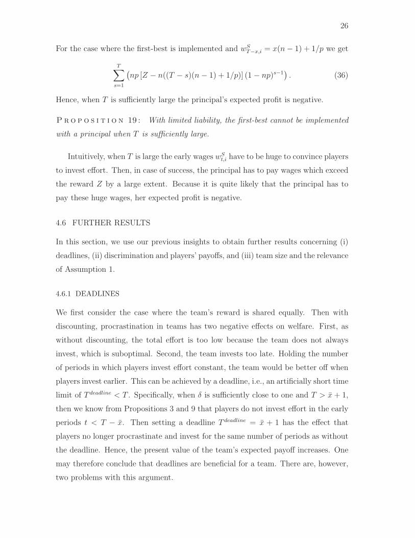
For the case where the first-best is implemented and wST−x,i = x(n− 1) + 1/p we get

T∑

s=1

(np [Z − n((T − s)(n− 1) + 1/p)] (1− np)s−1

). (36)

Hence, when T is sufficiently large the principal’s expected profit is negative.

P r o p o s i t i o n 19 : With limited liability, the first-best cannot be implemented

with a principal when T is sufficiently large.

Intuitively, when T is large the early wages wSt,i have to be huge to convince players

to invest effort. Then, in case of success, the principal has to pay wages which exceed

the reward Z by a large extent. Because it is quite likely that the principal has to

pay these huge wages, her expected profit is negative.

4.6 FURTHER RESULTS

In this section, we use our previous insights to obtain further results concerning (i)

deadlines, (ii) discrimination and players’ payoffs, and (iii) team size and the relevance

of Assumption 1.

4.6.1 DEADLINES

We first consider the case where the team’s reward is shared equally. Then with

discounting, procrastination in teams has two negative effects on welfare. First, as

without discounting, the total effort is too low because the team does not always

invest, which is suboptimal. Second, the team invests too late. Holding the number

of periods in which players invest effort constant, the team would be better off when

players invest earlier. This can be achieved by a deadline, i.e., an artificially short time

limit of T deadline < T . Specifically, when δ is sufficiently close to one and T > x+ 1,

then we know from Propositions 3 and 9 that players do not invest effort in the early

periods t < T − x. Then setting a deadline T deadline = x + 1 has the effect that

players no longer procrastinate and invest for the same number of periods as without

the deadline. Hence, the present value of the team’s expected payoff increases. One

may therefore conclude that deadlines are beneficial for a team. There are, however,

two problems with this argument.

27

First, deadlines are not renegotiation-proof. When the team arrives at period

T deadline and has no success, the expected payoff from obeying the deadline is zero,

while ignoring the deadline and continuing yields a positive expected payoff.

Second, designing an appropriate contract is a better measure to alleviate procras-

tination than a deadline, at least when δ is sufficiently close to one. We next prove

this claim. Denote the present value of the team’s expected payoff, measured at the

beginning of the game with the deadline, by∑

N CT deadline

1,i . A necessary condition for

T deadline to be optimal is that the team cannot improve by setting the deadline one

period longer. When the team does this, the Bellman equation is

∑

N

CT deadline+11,i = e1pZ + (1− e1p)δ

∑

N

CT deadline+12,i − e1. (37)

Note that the team can at least implement e1 = n − 1; this is implemented by

setting wS1,i sufficiently large for players i ∈ {2, ..., n} and wS

1,1 such that the budget is

balanced. Moreover, the team can use the same contract as when the deadline would

be T deadline, with one period delay from period 2 on. All this implies that

∑

N

CT deadline+11,i ≥ (n− 1)pZ + (1− (n− 1)p)δ

∑

N

CT deadline

1,i − (n− 1). (38)

Therefore, when

(n− 1)pZ + (1− (n− 1)p)δ∑

N

CT deadline

1,i − (n− 1) >∑

N

CT deadline

1,i , (39)

then the deadline T deadline cannot be optimal. Rewriting (39) yields

Z − 1/p >1− δ

p(n− 1)

∑

N

CT deadline

1,i + δ∑

N

CT deadline

1,i . (40)

∑

N CT deadline

1,i is maximal when the team is able to implement the first-best. Hence,

we get from (12) that

∑

N

CT deadline

1,i ≤∑

N

CT deadline

1,i = (npZ − n)1− (δ(1− np))T

deadline

1− δ(1− np). (41)

Therefore,∑

N CT deadline

1,i << Z − 1/p. This implies that (40) is satisfied, at least for

δ sufficiently close to 1. We conclude that a sufficient condition that players do not

want to use a deadline—even if they could commit to it—is that δ is sufficiently close

to 1.

28

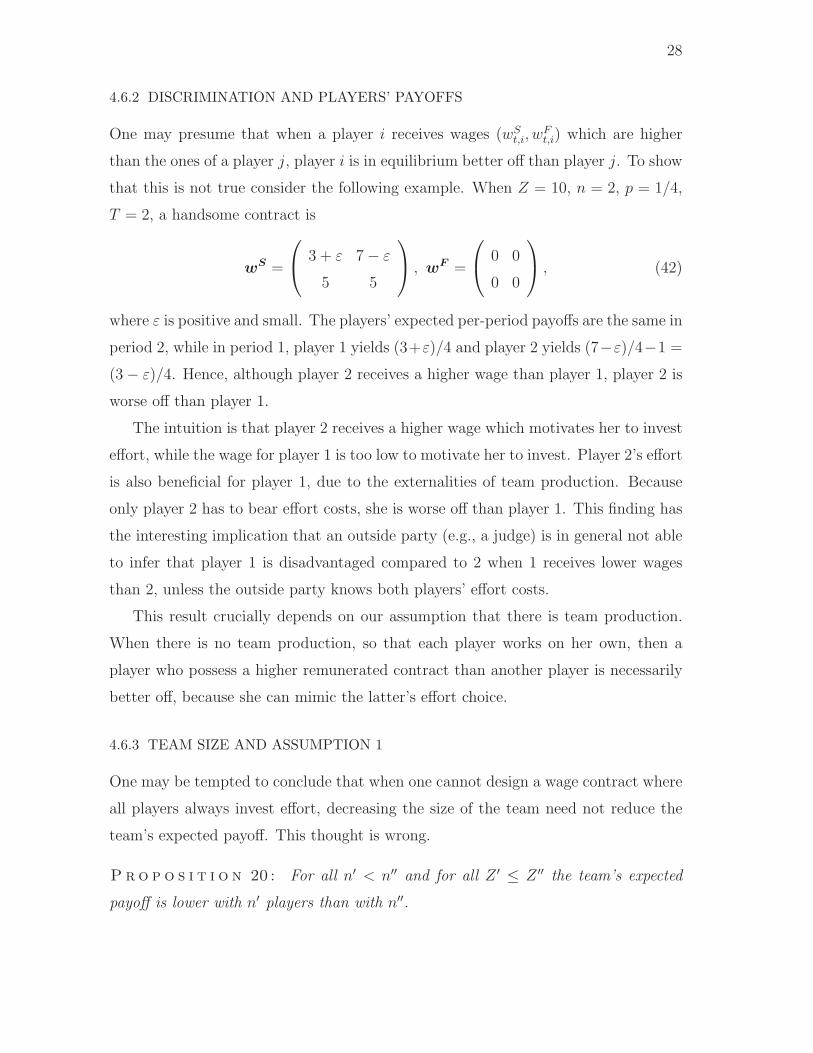
4.6.2 DISCRIMINATION AND PLAYERS’ PAYOFFS

One may presume that when a player i receives wages (wSt,i, w

Ft,i) which are higher

than the ones of a player j, player i is in equilibrium better off than player j. To show

that this is not true consider the following example. When Z = 10, n = 2, p = 1/4,

T = 2, a handsome contract is

wS =

3 + ε 7− ε

5 5

, wF =

0 0

0 0

, (42)

where ε is positive and small. The players’ expected per-period payoffs are the same in

period 2, while in period 1, player 1 yields (3+ε)/4 and player 2 yields (7−ε)/4−1 =

(3− ε)/4. Hence, although player 2 receives a higher wage than player 1, player 2 is

worse off than player 1.

The intuition is that player 2 receives a higher wage which motivates her to invest

effort, while the wage for player 1 is too low to motivate her to invest. Player 2’s effort

is also beneficial for player 1, due to the externalities of team production. Because

only player 2 has to bear effort costs, she is worse off than player 1. This finding has

the interesting implication that an outside party (e.g., a judge) is in general not able

to infer that player 1 is disadvantaged compared to 2 when 1 receives lower wages

than 2, unless the outside party knows both players’ effort costs.

This result crucially depends on our assumption that there is team production.

When there is no team production, so that each player works on her own, then a

player who possess a higher remunerated contract than another player is necessarily

better off, because she can mimic the latter’s effort choice.

4.6.3 TEAM SIZE AND ASSUMPTION 1

One may be tempted to conclude that when one cannot design a wage contract where

all players always invest effort, decreasing the size of the team need not reduce the

team’s expected payoff. This thought is wrong.

P r o p o s i t i o n 20 : For all n′ < n′′ and for all Z ′ ≤ Z ′′ the team’s expected

payoff is lower with n′ players than with n′′.

29

The idea is that when the team optimally designs the wage contract, then the

implemented team effort et is weakly lower for all periods, and strictly lower for some

periods with a small team than with a large team. This deteriorates the team’s

expected payoff. These arguments also imply that when the team designs the wage

contract optimally, larger teams more likely solve the task. This result is in contrast

to the one with an equal-sharing contract, see Proposition 5.

What happens when Assumption 1 is violated because pz < 1? Then with the

equal-sharing contract no player ever invests. A team can implement that n − 1

players invest effort in all periods by designing a discriminatory contract, where—

just like in the early periods with a handsome contract—one player acts as a quasi-

principal. This contract is beneficial for the team if Zp > 1. By arguments similar

to the ones where Assumption 1 holds, this contract can be shown to be second-best

and renegotiation-proof. Although a larger team never yields a lower expected team

payoff than a smaller team (because it can mimic the effort profile of a smaller team),

there are constellations where a larger team may yield the same expected payoff as a

smaller team. A simple example is when T = 1, n′/p ≤ Z ′ = Z ′′ < (n′ + 1)/p. Then

with n′ players e1 = n′ is implementable, while with n′′ = n′ + 1 players one can at

most implement e1 = n′′ − 1 = n′, too.

5 EXTENSIONS

In this section, we offer several extensions. Throughout we assume that the reward

is shared equally. In Section 5.1, we suppose that players have social preferences. We

explore how teams are optimally designed when players are heterogenous with respect

to their social preferences and show that it is better to have teams with heterogenous

players than to have homogenous teams. In Section 5.2, we explore the case when

there is no time limit for solving the task. We characterize the symmetric Markov

perfect equilibrium. In Section 5.3, we allow for very general success functions and

consider the cases where the success function is superadditive or subadditive. In

Section 5.4, we suppose that the reward which the team obtains for solving the task

declines over time. We then show that there might be an artificial time limit and

that players might not invest effort when the reward is high, but invest effort when it

30

is rather low. In Section 5.5, we assume that there are several tasks which the team

can solve. We show that when there are less tasks than periods in which the team

can work on the tasks, the team might procrastinate.

5.1 SOCIAL PREFERENCES AND TEAM DESIGN

Numerous experiments show that many people are not purely self-interested. Moti-

vated by these findings we assume in this section that players have social preferences.24

Suppose that each player puts a weight of φ ∈ [0, 1] on the other players’ material

payoffs.25 The parameter φ captures how much a player cares about the other players’

well-being, compared to her own well-being. A purely selfish player is characterized

by φ = 0, whereas for an altruistic player φ = 1.

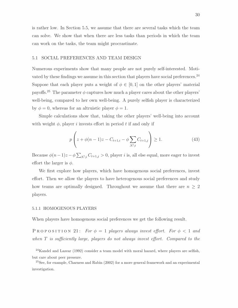
Simple calculations show that, taking the other players’ well-being into account

with weight φ, player i invests effort in period t if and only if

p

z + φ(n− 1)z − Ct+1,i − φ∑

N\i

Ct+1,j

≥ 1. (43)

Because φ(n−1)z−φ∑

N\i Ct+1,j > 0, player i is, all else equal, more eager to invest

effort the larger is φ.

We first explore how players, which have homogenous social preferences, invest

effort. Then we allow the players to have heterogenous social preferences and study

how teams are optimally designed. Throughout we assume that there are n ≥ 2

players.

5.1.1 HOMOGENOUS PLAYERS

When players have homogenous social preferences we get the following result.

P r o p o s i t i o n 21 : For φ = 1 players always invest effort. For φ < 1 and

when T is sufficiently large, players do not always invest effort. Compared to the

24Kandel and Lazear (1992) consider a team model with moral hazard, where players are selfish,

but care about peer pressure.25See, for example, Charness and Rabin (2002) for a more general framework and an experimental

investigation.

31

case where players are purely selfish (φ = 0), social players (φ > 0) begin to invest

effort weakly earlier.

For φ = 1 players are altruistic and always invest, because this maximizes welfare.

For φ < 1 and when the time limit T is sufficiently long we get again the result that the

team procrastinates. But as the last part of Proposition 21 clarifies, procrastination

is alleviated by social preferences.

5.1.2 HETEROGENOUS PLAYERS

We now suppose that players have heterogeneous social preferences. A classical issue

of economics (e.g., Lazear 1989 and Jeon 1996) is how players should be grouped

together, i.e., how teams should be designed. Suppose there are two players who are

purely selfish (φ = 0) and two social players with φ = φ ∈ (0, 1). How should one

form two teams, each consisting of two players?

When a player decides to invest in period t, then the expected payoff must be

at least as great as the one from not doing so. Moreover, we know from before that

it is beneficial for a player’s material well-being when another one invests. Both

arguments imply that Ct,i + φiCt,−i ≥ Ct+1,i + φiCt+1,−i when some player invests

in t. When no player invests then Ct,i + φiCt,−i = Ct+1,i + φiCt+1,−i. Together with

(43) these findings imply that all players’ strategies are simple threshold rules which

specify when a player starts to invest. Denote the period in which player i starts to

invest by t(φi, φ−i), where φ−i is the social preference parameter of the teammate.

From before we know that a social player is more eager to invest effort than a selfish

player. Hence, t(0, φ−i) ≥ t(φ, φ−i). We get two further results.

L e m m a 3: t(0, 0) = t(0, φ) and t(φ, 0) ≤ t(φ, φ).

That is, a selfish player invests rather late—due to t(0, φ−i) ≥ t(φ, φ−i)—and her

behavior is not influenced whether she is matched with another selfish player or a

social player. A social player i begins to invest earlier. When matched with a selfish

player the term Ct+1,i+φiCt+1,−i is rather low because the selfish player invests rather

late. That is why a social player begins to invest earlier when matched with a selfish

player than when matched with another social player.

32

We next explore whether it is better to have two homogenous teams (one with

social and one with selfish players) or two heterogenous teams (each consisting of a

social and a selfish player).

P r o p o s i t i o n 22 : The aggregated expected payoff is at least as high with het-

erogenous teams than with homogenous teams.

From Lemma 3 we know that a social player begins to invest rather late when

matched with another social player, compared to the case when matched with a selfish

player. This effect can be exploited by having heterogenous teams. Then we have—on

average—more investments than when teams are homogenous.

An Example.— Suppose that z = 5, p = 1/4, T = 3, and φ = 1/4. Consider first

the case with a team consisting of two selfish players. They invest in t = 3 because

p(z − 0) ≥ 1. Hence, C3,i = 2pz − 1 = 3/2. Given this, players do not invest in t = 2

because p(z − C3,i) = 7/8 < 1 and for the same reason not in t = 1. Hence, the

expected payoff of the team, measured at the beginning of the game, is 2C3,i = 3.

Next consider a team with two social players. Obviously, players invest in t = 3

and C3,i = 3/2. In t = 2, players also invest because p(z + φz − C3,i − φC3,i) =

35/32 ≥ 1. Hence, C2,i = 2pz − 1 + (1− 2p)C3,i = 9/4. In t = 1, the players do not

invest because p(z + φz − C2,i − φC2,i) = 55/64 < 1. Hence, the expected payoff of

the team, measured at the beginning of the game, is 2C2,i = 9/2.

Finally, in a heterogenous team players obviously invest in t = 3 and hence C3,i =

3/2. Denote the social player as 1 and the selfish player as 2. Player 2 does not

invest in t = 2 because p(z − C3,2) = 7/8 < 1. Player 1 invests in t = 2 because

p(z + φz − C3,1 − φC3,2

)= 35/32 ≥ 1. Hence, C2,1 = pz−1+(1−p)C3,1 = 11/8 and

C2,2 = pz+(1−p)C3,2 = 19/8. In t = 1, player 2 does not invest because p(z−C2,2) =

21/32 < 1. But player 1 invests because p(z + φz − C2,1 − φC2,2

)= 137/128 ≥ 1.

Hence, C1,1 = pz − 1 + (1 − p)C2,1 = 41/32 and C1,2 = pz + (1 − p)C2,2 = 97/32.

Therefore, having two heterogenous teams leads to an aggregated expected payoff,

measured at the beginning of the game, of 2(41/32+ 97/32) = 69/8, whereas for two

homogenous teams we only have 3 + 9/2 = 60/8.

33

5.2 INFINITE HORIZON

Previously, we assumed that there is a finite time limit. We next suppose that there

is no time limit. While in the model with a time limit the case with continuous effort

is generally intractable (except when effort costs are linear, only numerical results

can be obtained), this is not true when there is no time limit.

We measure effort in “probability units” of success: there is success in period t

with probability∑

N et,i and failure otherwise, where et,i ∈ R+. Effort causes private

costs of k(et,i), with k(0) = 0, k′ > 0, and k′′ > 0.26 To guarantee inner solutions we

assume that limet,i→0 k′(et,i) = 0 and limet,i→1/n k(et,i) = ∞.

The following Bellman equation holds:

Ct,i =∑

N

et,jz +

(

1−∑

N

et,j

)

δCt+1,i − k(et,i). (BELLMAN)

Player i chooses effort et,i to maximize Ct,i. The resulting first-order condition or

incentive constraint is

z − δCt+1,i = k′(et,i). (IC)

We concentrate on symmetric Markov perfect equilibria (SMPE). We say that

an equilibrium is symmetric if all players choose the same investment in each period

(but the investment may depend on the period). A strategy is Markov if it does

not depend on state variables that are functions of the history of the game, except

the ones which affect payoffs. A Markov perfect equilibrium (MPE) is then a profile

of Markov strategies that yields a Nash equilibrium in every proper subgame (cf.

Fudenberg and Tirole 1991).

When the game has not ended in period t, then the team had no success until t.

The history of the team is hence the series of failures it has experienced. Because

prior failures do not affect current or future payoffs, a MPE specifies the same effort

choice for a player in every period, given that the game has not yet ended.

In a SMPE a player chooses not only the same effort in every period, but all

players choose the same effort. Formally, et,i = eSMPE for all i ∈ N and all t ∈ N.

26Having convex effort costs is highly plausible and standard in agency theory. In most of our

analysis nothing changes when effort costs are linear.

34

Because effort is constant in all periods and the same for all players we get from

(BELLMAN) that Ct,i = CSMPE for all i ∈ N and all t ∈ N. Hence, (BELLMAN)

can be rewritten as

CSMPE =neSMPEz − k(eSMPE)

1− δ + δneSMPE(B SMPE)

and (IC) as

z − δCSMPE = k′(eSMPE). (IC SMPE)

It is useful to determine the first-best benchmark.

L e m m a 4: In the first-best,

eFB = argmaxnez − k(e)

1− δ + δne(44)

and

CFB =neFBz − k(eFB)

1− δ + δneFB. (45)

P r o p o s i t i o n 23 : There always exists a SMPE. The SMPE is unique. eSMPE

and CSMPE solve (B SMPE) and (IC SMPE).

The next result shows that only when there is a single player the investments

in effort are first-best. Otherwise, the players underinvest. See Figure 1 for an

illustration.

P r o p o s i t i o n 24 : Keep z fixed. eSMPE is decreasing in n, while eFB is

increasing in n. For n = 1, eSMPE = eFB and CSMPE = CFB. Otherwise,

eSMPE < eFB and CSMPE < CFB. CSMPE is increasing in n.

The intuition why effort eSMPE is decreasing in the number of players n is that

the future externalities arising from team production are greater the larger the team

is. In a larger team a player has therefore less incentives to invest effort. This holds

despite that the per-capita reward z is kept fixed. The reason why the first-best effort

eFB is increasing in n is that in a larger team the team’s total reward nz is increasing

in n, keeping z fixed. Therefore, higher investments in effort are efficient.

We next explore the comparative statics with respect to the per-capita reward z.

When one increases the size of a team it may be plausible that z decreases. We get

thatdCSMPE

dz

∣∣∣∣(IC SMPE)

=1

δ>

ne

1− δ + δne=

dCSMPE

dz

∣∣∣∣(B SMPE)

. (46)

35

C

0

(ICSM

PE)

(BSM

PE)n=1

(BSM

PE)n=2

(BSMPE)n=3

eFBn=1

eFBn=2 eFB

n=3

eSMPEn=2

eSMPEn=3

=eSMPEn=1

e

Figure 1: Only for n = 1 is the SMPE first-best.

Hence, lowering z, holding all else equal, decreases effort eSMPE and expected payoff

CSMPE, which is intuitive; see Figure 2 for the case n > 1.

The comparative statics with respect to the discount factor δ are interesting.

Because dCdδ

∣∣(IC SMPE)

< 0 and dCdδ

∣∣(B SMPE)

> 0 we get that deSMPE/dδ < 0. A

single player always chooses first-best effort; dCdδ

∣∣(B SMPE)

> 0 then implies that

dCSMPEn=1 /dδ > 0. Put differently, a single player benefits from a higher δ. With

several players this is not necessarily true. To see this, consider the case of quadratic

effort costs k(e) = e2/2. Using (B SMPE) and (IC SMPE) we get

eSMPE =−(1− δ) +

√

(1− δ)2 + 2δ(1− δ)z(2n− 1)

δ(2n− 1). (47)

Table 1 shows an example with n = 2 and z = 0.5, where players may benefit from a

lower δ: they are better off when δ = 0 than with δ ∈ {0.05, ..., 0.8}. The intuition

is that although players are, all else equal, better off with a higher δ, see (B SMPE),

36

0

(ICSM

PE)zlow

(ICSM

PE)zhigh

(BSM

PE)zlow

(BSM

PE)zhigh

C

e

A

B

Figure 2: Point A is the initial SMPE, point B the SMPE for a lower z.

they may reduce effort eSMPE so much that their expected payoff CSMPE is impaired.

δ 0 0.05 0.1 0.2 0.3 0.4 0.5

eSMPE 0.500 0.482 0.464 0.431 0.398 0.366 0.333

CSMPE 0.375 0.366 0.359 0.347 0.340 0.335 0.333

δ 0.6 0.7 0.8 0.9 0.95 0.99 →1

eSMPE 0.299 0.261 0.217 0.159 0.116 0.055 0.000

CSMPE 0.335 0.341 0.354 0.379 0.404 0.450 0.500

Table 1: Example with n = 2, z = 0.5, and k(e) = e2/2.

Interestingly, when there are several players, n > 1, making each player a residual

claimant (each receives Z in case of success and 0 in case of failure) is not enough

to motivate the players to invest first-best effort. To see this, adjust and combine

(IC SMPE) and (B SMPE) to get

Z − δneZ − k(e)

1− δ + δne= k′(e), (48)

37

which is solved by e. In the first-best we maxe CB(e, n) =nez−k(e)1−δ+δne

. Hence, eFB solves

Z − δneZ − nk(e)

1− δ + δne= k′(e). (49)

Because k′′ > 0, players underinvests when they are residual claimants: e < eFB.

The reason for this result is that a player does not take into account that solving the

task now saves n− 1 other players the future effort costs from investing.

Although the SMPE is appealing, there may also exists other equilibria. In Ap-

pendix B, we show, by means of two examples, that there can be symmetric non-

Markov perfect equilibria as well as asymmetric Markov perfect equilibria. Interest-

ingly, see Appendix B, players may be better off by playing a non-Markov perfect

equilibrium than by playing a SMPE.

5.3 MORE GENERAL SUCCESS FUNCTIONS

Suppose that the task is solved in period t with probability P (et). We assume that

when no player invests effort, then there is success with probability zero, that success

is more likely when more players invest effort, that success is also possible when all

but one player of the team invest effort, and that success is not guaranteed even when

all players invest.

A s s u m p t i o n 2 : Given n ≥ 2. P (0) = 0, P ′(et) > 0, P (n − 1) > 0, and

P (n) < 1.

The continuation payoff, given that all players invest effort from t until T , is

Ct,i = (P (n)z − 1)1− (1− P (n))T−t+1

P (n), (50)

which is just a slightly adapted version of (3). For the limit case

limT→∞

Ct+1,i = z −1

P (n). (51)

It is easy to show that, given that all other players invest in period t, it is optimal

for a player i to invest effort as well if and only if

(P (n)− P (n− 1)) (z − Ct+1,i) ≥ 1. (52)

38

For the limit case T → ∞ and when all players always invest (52) gets

1−P (n− 1)

P (n)< 1. (53)

Because Ct,i is continuous in T , we get the result that the team procrastinates when

the time limit is sufficiently long.

P r o p o s i t i o n 25 : Given Assumption 2 and that n ≥ 2. When the time limit

T is sufficiently long, not all players always invest effort.

Observe that when Assumption 2 is violated because P (n − 1) = 0, the team’s

problem collapses to a coordination problem. Regardless of T , it is an equilibrium

that all players always invest when P (n)z ≥ 1; i.e., there is no procrastination. It is,

however, also an equilibrium that nobody ever invests.

We next assume that the success function P is either super- or subadditive.

D e f i n i t i o n 3 : The function P is superadditive (subadditive) if P (e′ + e′′) ≥

(≤) P (e′) + P (e′′) for all e′, e′′ ≥ 0.

Superadditivity captures the idea that success is more likely when two groups of

players invest effort at the same time than when the groups invest at different times.

Then it is optimal to pool forces. Note that one reason a team may form in the first

place may be superadditivity.

From (52) we see that, given some P (n), procrastination is more likely, in the sense

that it occurs for a larger parameter set, the smaller is (P (n)−P (n− 1)). Therefore,

with subadditivity procrastination is more likely than with superadditivity. The

intuition is that with subadditivity the player is inclined to invest no effort, given

that all other players invest, because the probability of success is not much higher

when she invests, namely P (n), compared to the case when she does not invest,

namely P (n− 1).

With subadditivity one may get asymmetric equilibria, where some players invest

effort, while others do not. A simple example is

P (et) =

etp , for et < n,

(n− 1)p+ ε, for et = n,

39

where p ∈ (0, 1/(n−1)) and ε is positive and small. Then it cannot be an equilibrium

that all players invest for sure in some period. Additionally, there may also be

equilibria in mixed strategies.

5.4 DECREASING REWARDS

We now suppose that the reward, which the team receives for solving the task, de-

creases with time. Formally, we assume that for all t ∈ {1, ..., T}, Zt > Zt+1. An

example where a decreasing reward is highly plausible is when the team’s task is to

obtain an innovation; it is usually at least weakly better to have an innovation earlier.

Recognize that once pzt < 1, where zt := Zt/n is the per-capita reward, nobody

will invest. Hence, when pzt < 1 holds for a t ≤ T , there is an artificial time limit

T art = max{t ∈ N|pzt ≥ 1}. Denote the minimum of the real and the artificial time

limit (if there is one) by Tmin := min{T, T art}.

We are interested whether the players always invest effort until Tmin. This holds

if and only if

p(zt − Ct+1,i) ≥ 1 (54)

for all t ≤ Tmin, where Ct+1,i is the continuation payoff when all players invest from

t+ 1 until Tmin and not afterwards. This continuation payoff evolves according to

Ct,i = npzt + (1− np)Ct+1,i. (55)

Because CTmin+1 = 0 we know that all players invest in period Tmin. When (54) fails

for a single t ≤ Tmin we know that players do not always invest until Tmin. Then,

because the reward is decreasing in time, we get the result that players do not only

invest too seldom, but also at the wrong time. For example, when they do not invest

in period t′ < Tmin it would collectively be better for the players to invest in t′ instead

of Tmin, because zt′ > zTmin .

An Example.— Suppose that n = 2, p = 1/4, T = 5, z1 = 6.5, z2 = 6, z3 = 5,

z4 = 3.5, and z5 = 3. Because pz4 < 1 and pz5 < 1 we have an artificial time

limit T art = 3. In t = 3, both players invest because 1/4 × (5 − 0) ≥ 1. This gives

a continuation payoff C3,i = 1/2 × 5 − 1 = 1.5. In t = 2, players invest because

1/4 × (6 − 1.5) ≥ 1, resulting in C2,i = 1/2 × 6 + 1/2 × 1.5 − 1 = 2.75. In t = 1,

players do not invest because 1/4× (6.5− 2.75) < 1.

40

5.5 MULTIPLE TASKS

We have assumed that the team has to perform one task. What happens when

there are several tasks? Suppose that tasks are homogenous. When there are at

least as many task as periods, then it is without loss of generality to assume that

the players work on a different task in every period. Then there is no scope for

procrastination, since current success or failure does not influence future investments

and payoffs. Otherwise, the team might procrastinate because future externalities

arising from team production make investing effort in the present unattractive. To

see this, consider the following example.

An Example.— There are two tasks, z ∈ [4, 6), n = 2, p = 1/4, and T = 3.

Denote the number of tasks which are not solved at the beginning of period t by

Ot. When O3 > 0, then the players invest effort in t = 3, because this yields an

additional expected payoff for a player of 1/4× z− 1 ≥ 0. In period 2, players invest

effort if O2 = 2: the game continues for sure until period 3 and the expected payoff

of period 3 stays unaffected of what happens in period 2; therefore investing effort

yields an additional expected payoff for a player of 1/4 × z − 1 ≥ 0. For O2 = 1

the continuation payoff of reaching period 3 with O3 = 1 is too large to motivate

players to invest effort in period 2; cf. Proposition 3. Given this, the continuation

payoff of reaching period 2 depends on O2: CO2=22,i = 2

(12z − 1

), CO2=1

2,i = 12z−1. The

additional expected payoff from investing effort in period 1 is

1/4× (z + C2,O2=1 − C2,O2=2)− 1 = z/8− 3/4, (56)

which is negative because z < 6. To sum up, players only invest effort in periods 2

and 3. So we have again the result that the team procrastinates.

6 CONCLUSION

In this paper we show that when players are remunerated equally and face a suffi-

ciently long time limit, they begin to invest effort rather late. Players procrastinate

to benefit from future externalities arising from team production. This is socially

inefficient, but individually rational. When players can design wage contracts they

can mitigate procrastination. By remunerating players differently, one can motivate

41

some players, though regularly not all of them, to invest effort also in early periods.

Limited liability or the threat of sabotage can severely restrict the team’s possibilities

to motivate many players. Further results are that players who earn higher wages can

be worse off than teammates with lower wages, that with social preferences teams

are optimally designed heterogeneously, and that present-biased preferences mitigate

procrastination.

We allowed players to have heterogenous social preferences. Players may also differ

with respect to other characteristics, like effort costs or the effectiveness of their effort.

Investigating these issues is an interesting topic for future research. When players

are little heterogenous, we suspect that, generically, all of our results stay valid. The

idea is that players are generically never indifferent, and therefore their decisions do

not change when there is little heterogeneity instead of homogeneity.

42

APPENDIX A: PROOFS

PROOF OF PROPOSITION 1

From (57), see below, we see that∑

N C1,i is maximized when e1 is chosen optimally

and when∑

N C2,i is maximized.∑

N C2,i is in turn maximized when e2 is chosen

optimally and when∑

N C3,i is maximized. These arguments can be repeated and

imply that we can solve the social planner’s problem by backward induction.

For the special case where n = 1 and pZ = 1 we see from (2) that welfare∑

N C1,i is zero for all investment profiles. We now consider the case where this is

not true. Assumption 1 implies that then Z−1/p > 0. In period t, the social planner

maximizes, cf. (1),

∑

N

Ct,i = etpZ + (1− etp)∑

N

Ct+1,i − et. (57)

The derivative isd∑

N Ct,i

det= pZ − p

∑

N

Ct+1,i − 1. (58)

A sufficient condition for this to be positive, and therefore for et = n to be optimal,

is that∑

N

Ct+1,i < Z − 1/p. (59)

We start with period T . Because CT+1,i = 0 and Z − 1/p > 0 holds, inequality

(59) is satisfied and hence eT = n.

From (57) we get

∑

N

Ct,i = etp (Z − 1/p) + (1− etp)∑

N

Ct+1,i. (60)

Next, consider period t = T − 1. From (60) we see that∑

N CT,i is equal to the

weighted average of Z − 1/p and∑

N CT+1,i. Because∑

N CT+1,i = 0,∑

N CT,i is

lower than Z − 1/p. This implies that (59) is satisfied and the social planner sets

eT−1 = n.

Next, consider period t = T − 2. From (60) we see that∑

N CT−1,i is equal to the

weighted average of Z − 1/p and∑

N CT,i. Because∑

N CT,i is lower than Z − 1/p,

43

∑

N CT−1,i is lower than Z − 1/p, too. This implies that (59) is satisfied and the

social planner sets eT−2 = n.

These arguments can be repeated to show that the social planner always sets

et = n.

To prove the last part of the proposition note that because in the first-best all

players always invest we have∑

N Ct+1,i ≤∑

N Ct+1,i < Z − 1/p, where the last

inequality follows from the arguments before. Hence, (58) is positive and implies

that∑

N Ct,i is increasing in et. From (57),∑

N Ct,i is increasing in∑

N Ct+1,i, which

is in turn increasing in∑

N Ct+2,i, and so on. Hence,∑

N Ct,i increases with a higher

level of effort es, where s ≥ t. �

PROOF OF LEMMA 2

Part (i). In period T , all players face the same tradeoff: from Lemma 1 a player

invest in T if and only if p (z − CT+1,i) ≥ 1. Therefore, in T all players choose the

same investment. Because of this, CT,i is the same for all players. Hence, in period

T − 1 they again face the same tradeoff and therefore choose the same investment.

These arguments can be repeated, which establishes that all players choose the same

investment in every period.

Part (ii). When et = 0 it holds that Ct,i = Ct+1,i, see (1).

Part (iii). From Proposition 1 we know that∑

N Ct,i increases with et. Parts (i)

and (ii) imply that when players invest, Ct,i > Ct+1,i must hold.

Part (iv). When players always invest from t on then, by definition, Ct,i = Ct,i.

Otherwise, Proposition 1 implies that∑

N Ct,i <∑

N Ct,i. Part (i) then yields Ct,i <

Ct,i. �

PROOF OF PROPOSITION 3

From Lemma 1 it follows that players invest effort in period t if and only if the

continuation payoff of t + 1 is sufficiently low. From Lemma 2 we know that the

continuation payoff is nonincreasing in t. Therefore, one of the following patterns has

to hold: the players always invest effort or they do not invest effort until some period,

and always invest effort from this period on.

44

Due to p(

z − CT+1,i

)

≥ 1 and p(

z − limT→∞ Ct,i

)

< 1 we know that there must

exist a x such that

p(

z − CT−x,i

)!= 1, (61)

where t = T − x is now treated as a continuous variable which is possibly below 1.

With help of (3) we can solve (61) for

x =ln(n− 1)− ln(npz − 1)

ln(1− np)− 1, (62)

where ln is the natural logarithm.

It is useful to define

x := x+ 1. (63)

When T ≤ x+1, we claim that then p (z − Ct+1,i) ≥ 1 for all t ≥ 1. From Lemma

2 we know that Ct,i ≤ Ct,i and that Ct,i is decreasing in t. So when we can show that

p(

z − C2,i

)

≥ 1, (64)

then the claim is true. Inequality (64) indeed holds because C2,i ≤ CT−x,i due to

2 ≥ T − x ⇐⇒ T ≤ x+ 1 and the finding that Ct,i is decreasing in t.

We finally prove part (ii), where T > x + 1. We first show that players invest

effort in the periods t ≥ T − x. This requires that p (z − Ct+1,i) ≥ 1 for all t ≥ T − x.

This is indeed true because

Ct+1,i ≤ Ct+1,i ≤ CT−x,i, (65)

where the first inequality follows from Lemma 2 and the second from the finding that

Ct,i is decreasing in t and the fact that t+ 1 ≥ T − x ⇐⇒ t ≥ T − x.

We claimed that players do not invest effort in periods t < T − x. Denote t′ =

min{t|t ≥ T − x, t ∈ N}. That is, t′ is the lowest natural number for which Ct′+1,i ≤

CT−x,i. Hence, from Lemma 2,

Ct′,i > CT−x,i. (66)

From before we know that players invest effort for all periods t ≥ t′. Hence, Ct′,i =

Ct′,i. Together with (61) and (66) this implies that

p (z − Ct′,i) < 1. (67)

45

Hence, players do not invest in period t′ − 1. From Lemma 2 we know that the

continuation payoff is nonincreasing in t. Hence, players do not invest effort in periods

t < T − x. �

PROOF OF PROPOSITION 4

dx

dz=

<0︷ ︸︸ ︷

−np

npz − 1

<0︷ ︸︸ ︷

ln(1− np)

(ln(1− np))2︸ ︷︷ ︸

>0

> 0. (68)

Fix z.

dx

dn=

>0︷ ︸︸ ︷

1

(ln(1− np))2×

(1

n− 1−

pz

npz − 1

)

︸ ︷︷ ︸

>0

ln(1− np)︸ ︷︷ ︸

<0

+(ln(n− 1)− ln(npz − 1))︸ ︷︷ ︸

<0

p

1− np︸ ︷︷ ︸

>0

. (69)

Hence, dxdn

< 0 when z is fixed.

We fix Z and assume that Assumption 1 remains valid. With fixed Z dx/dn < 0

follows from dx/dn < 0 when fixing z and that dx/− dz < 0. �

PROOF OF PROPOSITION 5

From Proposition 3, players only invest in the last T period(s), where T := #{t|T ≥

t ≥ T − x, t ≥ 1}. Therefore, the likelihood that the task is solved during the whole

game is

1− (1− np)T . (70)

This probability is bounded away from 1 even when T is large.

In contrast, a single player always invests, see Proposition 2. The likelihood that

the task is solved during the whole game is

1− (1− p)T . (71)

46

Therefore, when T is sufficiently large, the probability of solving the task sometimes

is strictly higher for n = 1 than with n ≥ 2; compare (70) and (71).

When T is sufficiently small, for example when T = 1, then n ≥ 2 players more

likely solve the task than a single player; compare again (70) and (71). �

PROOF OF PROPOSITION 6

We only have to slightly adjust the proof of Proposition 1 by replacing the equality

in (60) by an inequality:

∑

N

Ct,i = etpZ+(1− etp)δ∑

N

Ct+1,i− et < etp (Z − 1/p)+ (1− etp)∑

N

Ct+1,i. (72)

The arguments concerning the weighted average must then be slightly adjusted to

say that∑

N Ct,i is lower than the weighted average of Z − 1/p and∑

N Ct+1,i. �

PROOF OF PROPOSITION 7

The first part follows directly from the findings that with δ < 1 instead of δ = 1

(i) each player is more eager to invest when Ct+1,i is stable or is lower when δ < 1

instead of δ = 1, see (13) and (ii) for a given effort profile (e1, ..., eT ), Ct+1,i is lower

for δ < 1 than when δ = 1, see (11).

The second part of the proposition follows from (13): when δ → 0, players always

invest effort; for δ = 1 this is not necessarily true, cf. Proposition 3. �

PROOF OF PROPOSITION 8

Because all players choose the same investment in every period, Proposition 6 implies

that Ct+1,i ≤ Ct+1,i. From (12) we know that Ct+1,i < (npz−1) 11−δ(1−np)

for any finite

T . Hence, Ct+1,i < (npz − 1) 11−δ(1−np)

for any finite T .

Plugging Ct+1,i = (npz − 1) 11−δ(1−np)

into (13) yields

p(z − (npz − 1)1

1− δ(1− np))

?

≥ 1; (73)

δ solves this with equality.

For a given effort profile (e1, ..., eT ) the continuation payoff is lower when δ de-

creases, see (11), and for a lower δ and a lower continuation payoff (13) is more likely

47

satisfied. Hence, when δ ≤ δ then all players always invest effort. While for δ > δ

and T sufficiently large it cannot hold that all players always invest because then,

due to Ct,i → (npz − 1) 11−δ(1−np)

, (13) is violated. �

PROOF OF PROPOSITION 9

Whether a player invests or not is determined by (13). Suppose there is no discount-

ing. Because all players choose the same investment in every period, there are only

T formulas to consider (one formula in every period). Generically, no such formula

holds with equality, i.e., generically a player is never indifferent. Suppose now that

there is discounting. Formulas that hold with > for δ = 1 also hold with > with δ

close to 1. The same is true for formulas which hold with <. Hence, for δ ∈ (δ, 1)

the players’ investments are the same with discounting than without. �

PROOF OF PROPOSITION 10

Also with β−δ preferences the continuation payoffs are given by (11) and (12). What

changes is player i’s invest rule, see (16).

The term Ct+1,i is maximized for T → ∞ and when all players always invest.

Then

limT→∞

Ct+1,i = (npz − 1)1

1− δ(1− np). (74)

Plugging this into (16) yields

p

(

z − βδ(npz − 1)1

1− δ(1− np)

)

≥ 1 (75)

This is solved with equality for β = β. From (16) we see that players always invest

when β ≤ β.

While for β > β and T sufficiently large it cannot hold that all players always

invest because then, due to Ct,i → (npz − 1) 11−δ(1−np)

, (16) is violated. �

PROOF OF PROPOSITION 11

From the proof of Proposition 3 we know that the equal-sharing contract wSt,i = Z/n

and wFt,i = 0 implements the first-best if and only if for all t ∈ {1, ..., T}

p(z − Ct+1,i) ≥ 1. (76)

48

Suppose, contrary to our claim, that there exists a wage contract (wS,wF ) which

implements the first-best when it is not implementable with the equal-sharing con-

tract. When all players invest in t, then (20) has to be satisfied for all players. Hence,

p

(∑

N

wSt,i −

∑

N

wFt,i −

∑

N

Ct+1,i

)

≥ n. (77)

Using the budget balance conditions (22) and dividing by n yields

p

(

Z/n−∑

N

Ct+1,i/n

)

≥ 1. (78)

Because all players always invest and the budget is balanced,

∑

N

Ct+1,i/n = Ct+1,i. (79)

Hence, (78) gets

p(z − Ct+1,i) ≥ 1. (80)

Because (80) coincides with (76), (80) cannot hold for all t ∈ {1, ..., T} when (76)

does not. A contradiction.

The second part of the proposition directly follows from Proposition 3. �

PROOF OF PROPOSITION 13

Part 1. We claim that a necessary condition that another contract (wS,wF ) is better

than the handsome contract is that in more periods all players invest.

With the handsome contract n−1 players invest in the early periods and n in the

late periods. That is, the effort profile is (e1 = n− 1, ..., et−1 = n− 1, et = n, ..., eT =

n), with t = min{t ∈ N : t ≥ T − x}.

Suppose e′τ = n−1 and e′τ+1 = n for an effort profile and e′′τ = n and e′′τ+1 = n−1

for an alternatively one. All other effort levels are the same: e′t = e′′t for all t 6= τ, τ+1.

Hence,∑

N Cτ+2,i is the same for both effort profiles. Using (23) twice we get that

∑

N

C ′τ,i = (n−1)pZ−(n−1)+(1−(n−1)p)

(

npZ − n+ (1− np)∑

N

C ′τ+2,i

)

, (81)

∑

N

C ′′τ,i = npZ − n+ (1− np)

(

(n− 1)pZ − (n− 1) + (1− (n− 1)p)∑

N

C ′′τ+2,i

)

.

(82)

49

Because∑

N C ′τ+2,i =

∑

N C ′′τ+2,i, we have

∑

N C ′τ,i =

∑

N C ′′τ,i. Because before period

τ e′t = e′′t we get that∑

N C ′1,i =

∑

N C ′′1,i.

These arguments can be repeated for any type of permutation of the effort profile

(e1 = n − 1, ..., et−1 = n − 1, et = n, ..., eT = n). Hence, a necessary condition that

another contract (wS,wF ) is better than the handsome contract is that in more

periods all players invest.

Part 2. Denote by #t the number of periods from t until T in which all players

invest. Denote the number of periods in which all players invest with the equal-

sharing contract from period 1 to T by #ES. For the contract (wS,wF ) to be better

than the handsome contract, we know by Part 1 that the contract must induce in

more periods investments of all players than the handsome contract: #1 > #ES.

Denote the period in which for the contract (wS,wF ) we have #t = #ES + 1 by t.

We claim that∑

N CT−#ES+1,i is a lower bound for∑

N Ct+1,i. Because additional

effort is beneficial for the team’s expected payoff, see Proposition 1, we get the fol-

lowing insight. For any effort profile (et+1, ..., es, ..., eT ) for which there exists an es

which is 0 < es < n, with s ∈ [t + 1, T ], the team’s expected payoff∑

N Ct+1,i is

higher than for the effort profile (et+1, ..., es = 0, ..., eT ). When we want to minimize∑

N Ct+1,i, while holding #t+1 fixed, we set all es 6= n to 0. Then

∑

N

Ct+1,i =∑

N

CT−#t+1+1,i, (83)

where we have used that∑

N Ct,i =∑

N Ct+1,i when no player invests in a period t,

see (23). Plugging in #t+1 = #ES establishes that∑

N CT−#ES+1,i is a lower bound

for∑

N Ct+1,i.

Part 3. Because all players are required to invest in period t with the contract

(wS,wF ), it most hold for all players i ∈ N that

p(

wSt,i − wF

t,i − Ct+1,i

)

≥ 1, (84)

Summing over all players and using the budget balance constraints (22) yields

p(Z −∑

N

Ct+1,i) ≥ n. (85)

From Part 2 we know that∑

N CT−#ES+1,i is a lower bound for∑

N Ct+1,i. Hence,

50

also

p(Z −∑

N

CT−#ES+1,i) ≥ n (86)

must hold. Dividing (86) by n yields

p(z − CT−#ES+1,i) ≥ 1, (87)

where we have used that Ct,i is the same for all players, see (3).

By the construction of x we have that with the equal-sharing contract all players

invest for t ≥ T − x and players do not invest before. Hence, for all periods t < T − x

p(z − Ct+1,i) < 1. (88)

With the equal-sharing contract all players invest from only t until T . So that the

number of periods for which all players invest indeed coincides with #ES we must

have

T − t+ 1 = #ES ⇐⇒ t = T −#ES + 1. (89)

Because players do not invest with the equal-sharing contract in period t = t− 1, we

must have that, using (88) and (89),

p(z − CT−#ES+1,i) < 1. (90)

Hence, (87) cannot hold. A contradiction. �

PROOF OF PROPOSITION 14

Consider two different periods and two different time limits: (i) the team’s expected

payoff in period t′ with a time limit T ′ is∑

N CT=T ′

t′,i ; (ii) with t′′ = t′− t′+1 = 1 and

T ′′ = T ′−t′+1 it is∑

N CT=T ′′

1,i . Suppose that in both cases the team uses a handsome

contract. It is immediate that then∑

N CT=T ′

t′,i =∑

N CT=T ′′

1,i . By Proposition 13 the

handsome contract is second-best and so∑

N CT=T ′′

1,i is maximized. Hence, when the

team is in period t′ and the time limit is T ′ it cannot renegotiate to yield a higher

expected payoff for the team than with the handsome contract. This proves that the

handsome contract is renegotiation-proof.

To prove the second part of the proposition, suppose, contrary to our claim,

that there is another renegotiation-proof contract (wS ′,wF ′

) which is second-best

51

and implements another effort profile e = (e1, ..., et, ..., eT ). Because the handsome

contract is also second-best and it induces investment by all players in the late periods

t ≥ T − x, the contract (wS ′,wF ′

) must induce more investment in the early periods

and less in the late periods. Otherwise, the contract (wS ′,wF ′

) and the handsome

contract cannot both be second-best or both contracts would induce the same effort

profile. Given the contract (wS ′,wF ′

), once the first period with t ≥ T−x is reached,

the team can renegotiate the wage contract to the handsome contract (which induces

equal sharing in the remaining periods). Renegotiating the wage contract induces

a higher expected payoff for the team, because more players invest effort is some

period(s) s ≥ t, cf. Proposition 1. Hence, the team can make transfers so that all

players are better off due to renegotiation. This proves that the alternative contract

(wS ′,wF ′

) is not renegotiation-proof. �

PROOF OF PROPOSITION 16

Consider the following contract. For all periods and players wFt,i = 0. In the late

periods t ≥ T − x, use the equal-sharing contract: wSt,i = Z/2. In the early periods

t < T − x, use the alternating contract wSt,1 = Z and wS

t,2 = 0 for t even and wSt,1 = 0

and wSt,2 = Z for t uneven.

We now prove that this contract implements the second-best. In the late periods,

all players invest because in this periods the equal-sharing contract is used as in the

handsome contract, which implements the second-best; see Proposition 13.

Before we look at the early periods we have to restrict the continuation payoffs. It

is useful to compare the two-player problem with the problem of a single player who

faces the same parameter constellation. Observe that Cn=1T,1 = pZ − 1 = 2pZ/2− 1 =

Cn=2T,i . If period t < T is a late period we have for the single-player problem

Cn=1t,1 = pZ + (1− p)Cn=1

t+1,1 − 1 (91)

and for the two-player problem

Cn=2t,i = 2pZ/2 + (1− 2p)Cn=2

t+1,i − 1 = pZ + (1− 2p)Cn=2t+1,i − 1. (92)

Because Cn=2T,i ≤ Cn=1

T,1 , (91) and (92) imply that Cn=2T−1,i ≤ Cn=1

T−1,1. Repeating the

arguments leads to the conclusion that in all late periods Cn=2t,i ≤ Cn=1

t,1 .

52

We next look at the latest early period, called t. Player j is induced to invest

effort while player −j is not. Player j invests effort in this period if and only if, see

(20) and recall that wSt,j

= Z and wFt,j

= 0,

p(

Z − Cn=2t+1,j

) ?

≥ 1. (93)

We know that the single player invests effort which implies that

p(

Z − Cn=1t+1,1

)

≥ 1. (94)

Because we know from above that Cn=2t+1,j

≤ Cn=1t+1,1

, (93) has to be satisfied, too.

Consider next the period t−1, where player −j should invest effort and wSt−1,−j

=

Z and wFt−1,−j

= 0. Because player j may have success in period t, it holds that

Cn=2t,−j

< Cn=2t+1,j

. Therefore, the arguments from above can be repeated to show that

player −j invests effort in period t − 1. More generally, when player j invests effort

in an early period t, player −j also invests effort in period t− 1.

Consider next the period t − 2. It holds that player j’s continuation payoff of

reaching the next period t− 1 is lower than the one of a single player:

Cn=2t−1,j = (1− p)Cn=2

t,j = (1− p)(

pZ − 1 + (1− p)Cn=2t+1,j

)

≤ pZ − 1 + (1− p)(

pZ − 1 + (1− p)Cn=1t+1,1

)

= pZ − 1 + (1− p)Cn=1t,1 = Cn=1

t−1,1, (95)

where the first equality follows from wSt−1,j

= wFt−1,j

= 0 and that only player −j

invests effort in period t−1. The second equality uses that wSt,j

= Z and wFt,j

= 0 and

that only player j invests effort in period t. The inequality follows from our above

finding that Cn=2t+1,j

≤ Cn=1t+1,1

and that pZ ≥ 1.

Because the single player invests in period t− 2, we have

p(Z − Cn=1t−1,1) ≥ 1. (96)

Because Cn=2t−1,j

≤ Cn=1t−1,1

, also player j invests in period t− 2:

p(Z − Cn=2t−1,j) ≥ 1. (97)

The arguments can be repeated to show that j will invest in periods t− 4, t− 6, ... .

Trivially, a player i for whom wSt,i = wF

t,i = 0 does not invest effort in period t.

This proves the desired result. �

53

PROOF OF PROPOSITION 17

Part 1. We suppose that the second-best is implemented and let T be large. We

seek to find a necessary condition on how large Z has to be. We consider the relaxed

problem where∑

N wSt,i is constant and where

∑

N wSt,i ≤ Z. We want to set wages

wSt,i as low as possible and obtain minimal continuation payoffs.

Consider some t which is far away from T . Then in the second-best n− 1 players

invest effort. For a player i who invests effort in t we set the lowest possible wage,

given the incentive constraint (20),

wSt,i =

1

p+ Ct+1,i. (98)

Player i’s Bellman equation is

Ct,i = (n− 1)pwSt,i + (1− (n− 1)p)Ct+1,i − 1, (99)

where we have used that wFt,i = 0. Plugging (98) into (99) we get

Ct,i = n− 2 + Ct+1,i. (100)

There is also a player who does not invest effort in t. We call her player j(t). For this

player the Bellman equation is, setting wSt,j(t) as low as possible, namely wS

t,j(t) = 0,

Ct,j(t) = (1− (n− 1)p)Ct+1,j(t). (101)

Summing over all players we get, using (100) and (101),

∑

N

Ct,i = (n− 1)(n− 2) +∑

N

Ct+1,i − (n− 1)pCt+1,j(t). (102)

Because T is large, relatively to t, and we assumed that the second-best is imple-

mented we have∑

N Ct,i ≈∑

N Ct+1,i, where the failure gets arbitrarily small as T

gets larger, see (24). Hence, (102) gets

Ct+1,j(t) =n− 2

p+ ε1, (103)

where ε1 is arbitrarily small when T gets large.

Combining (101) and (103) yields

Ct,j(t) =n− 2

p− (n− 1)(n− 2) + ε2. (104)

54

Part 2. When should which player not invest effort? It is useful to define the

number of periods player i will invest effort uninterruptedly from period t on by dt,i.

For example, when j(t) = i we have dt,i = 0, when j(t) 6= i and j(t + 1) = i then

dt,i = 1, and so on. Then we get from (100) that

Ct,i = dt,i(n− 2) + Ct+dt,i,j(t+dt,i)=i. (105)

Note that due to limited liability continuation payoffs cannot be negative. Together

with∑

Ct,i < Z and (105) this implies that dt,i cannot be larger than Z/(n − 2);

otherwise Ct,i > Z.

Consider the problem of minimizing∑

Ct,i subject to (105) and that dt,i ≤ Z/(n−

2).

We claim that it is best to let in every period t until t + n − 1 another player

not invest effort. We prove by contradiction. When there is another schedule which

is better, then there must be a player i′ who does not invest in effort at least twice

between t and t + n − 1. Denote the period in which i′ does not invest effort the

second time by t′. There is also a player with the highest value of dt,i (from above we

know that dt,i ≤ Z/(n − 2)) which we call player i′′. She invests effort from t until

t+ dt,i′′ − 1, and does not invest in period t+ dt,i′′ . From (105) we get that

Ct,i′′ = dt,i′′(n− 2) + Ct+dt,i′′ ,j(t+dt,i′′ )=i′′ . (106)

If we change the schedule and let player i′′ not invest in period t′ then we get

Ct,i′′ = (t′ − t)(n− 2) + Ct′,j(t′)=i′′ . (107)

From (104) we see that Ct,j(t) is approximately constant for periods t until t + dt,i′ .

Hence,

(t′ − t)(n− 2) + Ct′,j(t′)=i′′ < dt,i′′(n− 2) + Ct+dt,i′′ ,j(t+dt,i′′ )=i′′ . (108)

Because for all other players of (105) is left unchanged,∑

N Ct,i is not minimized. A

contradiction.

Part 3. If in every period t until t + n − 1 another player does not invest effort

55

then we get from (105) that

∑

N

Ct,i = nCt,j(t) + (n− 2)∑

N

di,t + ε3

= nCt,j(t) + (n− 2)(0 + 1 + ...+ (n− 1)) + ε3

= nCt,j(t) + n(n− 2)n− 1

2+ ε3, (109)

where ε3 is arbitrarily small when T gets large.

Part 4. Plugging (104) into (109) yields∑

N

Ct,i = n(n− 2)/p− n(n− 1)(n− 2)/2 + ε4. (110)

Proposition 1 and (3) imply that∑

N Ct,i < Z − 1/p when∑

N wSt,i = Z, which also

hold when∑

N wSt,i ≤ Z. Hence, when

n(n− 2)/p− n(n− 1)(n− 2)/2 + ε4 ≥ Z − 1/p (111)

the second-best is not implementable when T is large. Rewriting (111), the second-

best with limited liability is not implementable with limited liability if T is sufficiently

large and

Z < Z := n(n− 2)/p+ 1/p− n(n− 1)(n− 2)/2. (112)

�

PROOF OF PROPOSITION 18

The proof is constructive. We construct a time-independent and nondiscriminatory

wage contract: wS = wSt,i and wF = wF

t,i for all i ∈ N and all t ∈ {1, ..., T}. When a

player invests effort in t, her expected payoff in period t is zero when

npwS + (1− np)wF − 1 = 0. (113)

When wages satisfy this for all periods, then Ct,i = 0 for all t ∈ {1, ..., T}, i ∈ N . To

induce always investment by all players we must have

p(wS − wF ) ≥ 1. (114)

The wages wS and wF solve (113) and (114) and induce that all players always invest.

By choosing the appropriate transfer which the principal has to pay to the team,

the team can make sure that principal’s expected profit is zero. Alternatively, one

can set the transfer equal to zero and adjust wS1,i and wF

1,i accordingly. �

56

PROOF OF PROPOSITION 20

Consider first the case where Z ′ = Z ′′. With n′ players we have en=n′

t ≤ n′. With

n′′ players and when T is sufficiently short, it is optimal for the team to use the

equal-sharing contract, see Proposition 11. Then et = n′′ for all t ∈ {1, ..., T}. When

T is longer, then the first-best cannot be implemented and the handsome contract is

second-best, see Proposition 13. It implements en=n′′

t = n′′ for periods t ≥ T − x and

en=n′′

t = n′′ − 1 for periods t < T − x.

From (24) we see that when en=n′′

t = en=n′

t then

n′′

∑

i=1

Cn=n′′

t,i =n′

∑

i=1

Cn=n′

t,i . (115)

Proposition 1 says that the team’s expected payoff∑n′′

i=1 Ct,i is increasing in es for all

s ≥ t. From before we know that en=n′′

s ≥ en=n′′

s for all periods and en=n′′

s > en=n′′

t for

some periods s ≥ t. Hence,

n′′

∑

i=1

Cn=n′′

t,i >

n′

∑

i=1

Cn=n′

t,i . (116)

From (24) we see that for a given effort profile e = (e1, ..., et, ..., eT ) the team’s

expected payoff∑n′′

i=1 Ct,i is increasing in Z. From Proposition 4 we know that

dx/dz > 0, which implies that for a higher Z an effort profile with weakly more

team effort et in every period can be implemented. Both effects imply that a team’s

expected payoff is increasing in Z. Hence, for all Z ′′ > Z ′ (116) holds. �

PROOF OF PROPOSITION 21

Part 1. For φ = 1, condition (43) gets

np (z − Ct+1,i) ≥ 1, (117)

where we have used that the continuation payoff is the same for all players. From

Lemma 2 we know that Ct+1,i ≤ Ct+1,i. Moreover, for any finite T , Ct+1,i is lower

than limT→∞ Ct+1,i = z − 1np. Because

np

(

z −

(

z −1

np

))

= 1, (118)

57

(117) always holds. Hence, all players always invest effort.

Part 2. For φ < 1, (43) gets

p(1 + φ(n− 1)) (z − Ct+1,i) ≥ 1. (119)

When all players always invest, Ct+1,i is arbitrarily close to limT→∞ Ct+1,i = z − 1np

when T is sufficiently large. Because

p(1 + φ(n− 1))

(

z −

(

z −1

np

))

=1 + φ(n− 1)

n< 1, (120)

it cannot hold that all players always invest when T is sufficiently large.

Part 3. Let x(φ) solve (119):

p(1 + φ(n− 1))(

z − CT−x(φ),i

)!= 1. (121)

Because CT−x(φ),i is increasing in x(φ), see (3), we get that x(φ) is increasing in φ.

Define x(φ) := x(φ) + 1. By the same arguments as in the proof of Proposition 3

we get that when the time limit is sufficiently short, namely T ≤ x(φ) + 1, then

players always invest effort and that when the time limit is sufficiently long, namely

T > x(φ) + 1, then players do not invest effort in periods t < T − x(φ) and invest

effort in the periods t ≥ T − x(φ). �

PROOF OF LEMMA 3

Start with the case φi, φ−i = 0. Ct(0,0),i > z − 1/p; otherwise player i would invest

in t(0, 0) − 1. Moreover, Ct(0,0)+1,i ≤ z − 1/p, otherwise player i would not invest in

period t(0, 0). Because t(0, φ−i) ≥ t(φ, φ−i), all players invest from period t(0, 0) to

T we get then with (43) and (3) that

Ct(0,0),i = (npz − 1)1− (1− np)T−t(0,0)+1

np> z − 1/p (122)

and

Ct(0,0)+1,i = (npz − 1)1− (1− np)T−t(0,0)

np≤ z − 1/p. (123)

Next consider the case φi = 0 and φ−i = φ. Because t(0, φ−i) ≥ t(φ, φ−i), all

players invest from period t(0, φ) to T . We must have

Ct(0,φ),i = (npz − 1)1− (1− np)T−t(0,φ)+1

np> z − 1/p. (124)

58

and

Ct(0,φ)+1,i = (npz − 1)1− (1− np)T−t(0,φ)

np≤ z − 1/p. (125)

Comparing (122)-(125) yields that we must have t(0, 0) = t(0, φ).

Finally, consider the remaining cases where φi = φ. By (43) it must hold that

p(z + φz − Ct+1,i − φCt+1,−i

)≥ 1 (126)

for all t ≥ t(φ, φ). Similarly,

p(z + φz − Ct+1,i − φCt+1,−i

)≥ 1 (127)

for all t ≥ t(φ, 0).

For the case φi = φ−i = φ all players invest from period t(φ, φ) until T . Hence,

Ct(φ,φ)+1,i + φCt(φ,φ)+1,−i = (1 + φ)Ct(φ,φ)+1,i. (128)

When φi = φ and φ−i = 0 we get that

Ct(φ,0)+1,i + φCt(φ,0)+1,−i = (1− φ)Ct(φ,0)+1,i + φ(Ct(φ,0)+1,i + Ct(φ,0)+1,−i

)

≤ (1−φ)Ct(φ,0)+1,i+φ2Ct(φ,0)+1,i ≤ (1−φ)Ct(φ,0)+1,i+φ2Ct(φ,0)+1,i = (1+φ)Ct(φ,0)+1,i,

(129)

where the first inequality follows from the finding that in the first-best, i.e., where

continuation payoffs are maximized, all players always invest effort. The second

inequality follows from t(0, φ−i) ≥ t(φ, φ−i) and the fact that player i is better off

when player −i invests than when not (player i invests from period t(φ, 0) on until

T , while this is not necessarily true for player −i).

From (128) and (129) and the finding that Ct+1,i is decreasing in t it follows that

whenever (126) holds for t, (127) has to hold, too. Hence, t(φ, 0) ≤ t(φ, φ). �

PROOF OF PROPOSITION 22

With homogenous teams their is one team with selfish players. This teams’ aggregated

expected payoff is, using (3),

2Ct(0,0),i = 2(2pz − 1)1− (1− 2p)T−t(0,0)+1

2p. (130)

59

For the team with the social players we have

2Ct(φ,φ),i = 2(2pz − 1)1− (1− 2p)T−t(φ,φ)+1

2p. (131)

When there are heterogenous teams, the each team’s expected payoff is, using (2),

(2pz − 1)1− (1− p)t(0,0)−t(φ,0)

p+ (1− p)t(0,0)−t(φ,0)2Ct(0,0),i, (132)

where the first part is the team’s expected payoff from periodst(φ, φ) until the period

before t(0, φ) = t(0, 0). This part diminishes when t(φ, φ) = t(0, 0). The second part

is the teams’ expected payoff from period t(0, φ) = t(0, 0) until T , where we have

taken into account that this period is reached only with probability (1− p)t(0,0)−t(φ,0).

We claim that having two heterogenous teams lead to a weakly higher aggregated

expected payoff than having one team with selfish players and one with social players:

(4pz − 2)1− (1− p)t(0,0)−t(φ,0)

p+ 2(1− p)t(0,0)−t(φ,0)(4pz − 2)

1− (1− 2p)T−t(0,0)+1

2p

≥ (4pz − 2)1− (1− 2p)T−t(0,0)+1

2p+ (4pz − 2)

1− (1− 2p)T−t(φ,φ)+1

2p. (133)

Dividing by (4pz − 2) and multiplying by 2p yields

2(

1− (1− p)t(0,0)−t(φ,0))

+ 2(1− p)t(0,0)−t(φ,0)(1− (1− 2p)T−t(0,0)+1

)

≥ 1− (1− 2p)T−t(0,0)+1 + 1− (1− 2p)T−t(φ,φ)+1. (134)

After simplifying and multiplying by −1 we get

2(1− p)t(0,0)−t(φ,0)(1− 2p)T−t(0,0)+1 ≤ (1− 2p)T−t(0,0)+1 + (1− 2p)T−t(φ,φ)+1. (135)

Dividing by (1− 2p)T−t(0,0)+1 yields

2(1− p)t(0,0)−t(φ,0) ≤ 1 + (1− 2p)t(0,0)−t(φ,φ). (136)

For t(0, 0) − t(φ, 0) = 0 or t(0, 0) − t(φ, 0) = 1 this formula holds with equality.

Because t(0, 0)− t(φ, 0) ≥ 0, it remains to check that it holds for t(0, 0)− t(φ, 0) ≥ 2.

It is useful to define g(p) = (1 − p)ζ . For ζ ≥ 2 this function is convex in p for

p ∈ [0, 1]. By convexity we have

g(p) ≤g(p+ ν) + g(p− ν)

2(137)

60

for all ν that satisfy p+ ν, p− ν ∈ [0, 1]. Hence, also

2g(p) ≤ g(2p) + g(0). (138)

Substituting t(0, 0)− t(φ, φ) for ζ proves the desired result. �

PROOF OF LEMMA 4

The first-best maximizes∑

N Ct,j. We claim that in the first-best all players choose

the same effort level in a period. Suppose not. Then there exist et,j 6= et,i. When

both players i and j chooseet,i+et,j

2,∑

N Ct,j is improved because 2k( et,i+et,j

2

)<

k(et,j) + k(et,i) due to k′′ > 0.

Note that Ct+1,j = Ct+1 for all j ∈ N because all players choose the same in-

vestment in a period, and this is true for all periods. Iterative use of (BELLMAN)

yields

Ct =∞∑

s=t

[

(nesz − k(es))s−1∏

r=t

δ(1− ner)

]

(139)

From (BELLMAN) we see that maxet Ct is increasing in Ct+1. Hence, to maximize

Ct we also maximize Ct+1. In period t we maximize Ct, see (139), over (et, et+1, ...),

in period t + 1 we maximize Ct+1 over (et+1, et+2, ...). So the problem is always the

same and hence Ct is maximized when always the same effort e is chosen. That is, in

the first-best all players choose eFB at every time which yields Ci,t = CFB. Rewriting

(BELLMAN) yields that

CFB =neFBz − k(eFB)

1− δ + δneFB, (140)

where eFB = argmaxnez−k(e)1−δ+δne

. �

PROOF OF PROPOSITION 23

It is useful to write the C which satisfies (B SMPE) as a function CB(e, n), where

B stands for the Bellman equation. Similarly, we write CIC(e) for the valuation C

satisfying (IC SMPE).

Existence. We first proof existence. Essentially, we want to show that CB(e) and

CIC(e) evolve like in Figure 3, where the functions CB(e, n) and CIC(e) cross at least

once.

61

We first determine how CB() evolves. For all n, we get that

d2CB(e, n)

de2∝ −k′′(e)

(1 + δ − δne)2

2δn− z(n− 1)(1− δ)− (n− 1)δc < 0. (141)

Because CB(0, n) = 0, dCB(0, n)/de > 0, CB(e, n) ≤ 0 for e sufficiently large, and

dCB(e, n)2/de2 < 0, see (141), we know that CB(e, n) is inverted-U shaped in e and

has a maximum at some e > 0, but no minimum. Moreover, CB(e, n) ≥ 0 if and only

if e ∈ [0, eB(n)], where eB(n) is implicitly defined by the e > 0 which solves

neB(n)z = k(eB(n)). (142)

Next we look how CIC() evolves. We get that

dCIC(e)

de= −

k′′(e)

δ< 0. (143)

Moreover, CIC(e) ≥ 0 if and only if e ≤ eIC , where eIC is implicitly defined by

z = k′(eIC). (144)

We get from (142) and (144) that

k(eB(n))

neB(n)= z = k′(eIC). (145)

Because k(e)/e < k′(e), k(e)/e and k′(e) are increasing in e, n ≥ 1, we must have

eB(n) > eIC .

Observe that CB(e, n) and CIC(e) are continuous in e and CB(0, n) = 0 < z/δ =

CIC(0). Together with the insights from before it follows that CB(e) and CIC(e) cross

at least once. That is, there exists a e such that CB(e, n) = CIC(e).

We have to check that for an e which solves CB(e, n) = CIC(e) the present value

of the player’s expected payoff is maximized not minimized. From (BELLMAN) we

see thatd2Ct,i

de2t,i= −k′′(et,i) < 0. (146)

Hence, the second-order condition is satisfied. Therefore, when e solves CB(e, n) =

CIC(e) we have a maximum and no minimum. Hence, a MPE always exists.

Uniqueness. Next we prove uniqueness. We want to show that CIC(e) and

CB(e, n) only intersect once, as in Figure 4.

62

0 e

C

eIC eB(n)

CIC(e)

CB(e, n)

Figure 3: Existence.

For n = 1 the effort level e which solves CB(e, 1) = CIC(e) is the one that

maximizes CB(e, 1): eFB(1) = argmaxeCB(e, 1). Because d2CB(e, n)/de2 < 0, it

follows that CB(e, 1) has no other extreme point. Consequently, CB(e, 1) = CIC(e) is

only solved by eFB(1) and no other e. That is, the MPE is unique when n = 1.

For more players (n > 1) we get that, given some e > 0,

dCB(e, n)

dn∝ z(1− δ) + δk(e) > 0. (147)

Note that CIC(e) does not change with n when z and all other parameters are kept

fix.

Because

dCB(e, n)

de∝ nz − δnz − k′(e)(1− δ + δne) + k(e)δn, (148)

eFB(n) is implicitly defined by

nz − δnz − k′(eFB(n))(1− δ + δneFB(n)) + k(eFB(n))δn = 0. (149)

By differentiating implicitly we get that

deFB(n)

dn= −

z − δz − k′(eFB(n))δeFB(n) + k(eFB(n))δ

−k′′(eFB(n))(1− δ + δneFB(n))

∝ z(1− δ)2 + k(eFB(n))δ(1− δ) > 0,

where we have used the first-order condition k′(eFB(n)) = nz − nδC.

63

We have that dCB(e, n)/de > 0 for all e < eFB(n). Because deFB(n)/dn > 0, for

n > 1, we get that dCB(e, n)/de > 0 for all e ≤ eFB(1). Therefore, CB(n) and CIC(n)

cross only once for e ∈ [0, eFB(1)]. Because (i) CB(e, 1) and CIC(e) do not cross for

any e > eFB(1) and (ii) CB(e, n) > CB(e, 1) for all n > 1, also CB(e, n) and CIC(e)

do not cross for any e > eFB(1). Hence, also for n > 1 the SMPE is unique. This is

illustrated in Figure 4.

C

0

CIC(e)

CB(e, 1)

CB(e, n > 1)

eFB(1) eFB(n > 1) e

Figure 4: Uniqueness.

�

PROOF OF PROPOSITION 24

We again write CB(e, n) for the C which satisfies (B SMPE) and CIC(e) for the C

satisfying (IC SMPE).

The results follow from, see especially the proof of Lemma 23, that (i) CB(e) is

inverted-U shaped in e, (ii) CB(e) is increasing in n for all e > 0, (iii) CIC(e) is

decreasing in e but constant in n, (iv) eFB is the SMPE with n = 1, and (v) eFB

is increasing in n. This is illustrated in Figure 1, which is in the main part of the

paper. �

64

APPENDIX B: SYMMETRIC NON-MPE AND

ASYMMETRIC MPE

In our model, players are symmetric and play every period the same game. Nonethe-

less, there may exist non-Markov perfect equilibria where players choose symmetric

investments as well as Markov perfect equilibria where players choose asymmetric

investments. The following examples are instructive.

SYMMETRIC NON-MARKOV PERFECT EQUILIBRIA

Suppose n = 2, δ = 0.5, and

k(e) =

(1− ε)e , for e ∈ [0, 0.1],

(1− ε) + (1 + ε)e, for e ∈ (0.1, 0, 2],

∞ , otherwise.

We want to construct an equilibrium where players choose

et =

0.2, for t uneven,

0 , for t even.

Suppose that this is an equilibrium. Then

Cuneven = 0.4× z + 0.6× 0.5× Ceven − 0.2 (150)

and

Ceven = 0.5× Cuneven. (151)

Inserting the latter in the former equation we get

Cuneven =0.4× z − 0.2

0.85(152)

and

Ceven =0.4× z − 0.2

1.7. (153)

To prove that this is an equilibrium we have to check the incentive constraints. When

t is uneven we need

z − 0.5× Ceven ≥ 1 + ε ⇐⇒ z −0.4× z − 0.2

3.4≥ 1 + ε (154)

65

and when t is even

z − 0.5× Cuneven ≤ 1− ε ⇐⇒ z −0.4× z − 0.2

1.7≤ 1− ε. (155)

Hence, for z ∈ (16/15, 15/13) and ε sufficiently small, both incentive constraints are

satisfied. Intuitively, in uneven periods players do not invest because the continuation

payoff of reaching the next period is high and the continuation payoff of even periods

is high because players invest a lot of effort. The intuition for why there is high

investment in even periods is vice versa.

Interestingly, players may be better off by playing a non-Markov perfect equilib-

rium than by playing a Markov perfect equilibrium. For example, when z = 1.1 and

ε = 0.02 then Cuneven ≈ 0.282 and Ceven ≈ 0.141. In the SMPE we have eSMPE = 0.1

and CSMPE ≈ 0.203. So at the beginning of the first period players prefer to coor-

dinate on playing the non-Markov perfect equilibrium than on playing the SMPE.

This is intuitive: in period 1, players invest much more in the non-Markov perfect

equilibrium than in the SMPE. Therefore, from the perspective of period 1, their

expected payoff is higher in the non-Markov perfect equilibrium than in the SMPE.

ASYMMETRIC MARKOV PERFECT EQUILIBRIA

Suppose that n = 2, δ = 0.5, and

k(e) =

e , for e ≤ 0.5,

∞, otherwise.

We want to check when et,1 = 0 and et,2 = 0.5 is a MPE. Then

Ct,1 =0.5× z

0.75=

2

3z (156)

and

Ct,2 =0.5× z − 0.5

0.75=

2

3z −

2

3. (157)

It remains to check that the players’ incentive constraints are satisfied. We need to

have

z − 0.5×2

3z ≤ 1 ⇐⇒ z ≤ 3/2 (158)

and

z − 0.5×

(2

3z −

2

3

)

≥ 1 ⇐⇒ z ≥ 1. (159)

66

Hence, for z ∈ [1, 1.5] et,1 = 0 and et,2 = 0.5 is a MPE.

The intuition is that because player 1 invests no effort her continuation payoff

Ct,1 is much higher than the one of player 2, Ct,2, who spends effort. Given this,

player 1 has no incentive to invest in t or in subsequent periods, whereas player 2 has

incentives to invest effort.

LITERATURE

Akerlof, George A. (1991). Procrastination and Obedience. American Economic Review Papers &

Proceedings 81, 1-19.

Alchian, Armen A. and Harold Demsetz (1972). Production, Information Costs, and Economic

Organization. American Economic Review 62, 777-795.

Andreoni, James (1995). Cooperation in Public-Goods Experiments: Kindness or Confusion? Amer-

ican Economic Review 85, 891-904.

Arrow, Kenneth J. (1998). What Has Economics to Say About Racial Discrimination? Journal of

Economic Perspectives 12, 91-100.

Becker, Gary (1957). The Economics of Discrimination. Chicago, Illinois, University of Chicago

Press.

Bonatti, Alessandro and Johannes Horner (forthcoming). Collaborating. American Economic Re-

view.

Charness, Gary and Matthew Rabin (2002). Understanding Social Preferences with Simple Tests.

Quarterly Journal of Economics 117, 817-869.

Cohen, Susan G. and Diane E. Bailey (1997). What Makes Teams Work: Group Effectiveness Re-

search form the Shop Floor to the Executive Suite. Journal of Management 23, 239-290.

Darity Jr., William A. and Patrick Mason (1998). Evidence on Discrimination in Employment:

Codes of Color, Codes of Gender. Journal of Economic Perspectives 12, 63-90.

Fudenberg, Drew and Jean Tirole (1991). Game Theory. Cambridge, Massachusetts, MIT Press.

Hamilton, Barton H., Jack A. Nickerson, and Hideo Owan (2003). Team Incentives and Worker

Heterogeneity: An Empirical Analysis of the Impact of Teams on Productivity and Participation.

Journal of Political Economy 111, 465-497.

Holmstrom, Bengt (1982). Moral Hazard in Teams. Bell Journal of Economics 13, 324-340.

Holzer, Harry and David Neumark (2000). Assessing Affirmative Action. Journal of Economic

Literature 38, 483-568.

Holzer, Harry J. and David Neumark (2006). Equal Employment Opportunity and Affirmative Ac-

tion. Handbook on the Economics of Discrimination, ed. William Rodgers. Great Britain, Edgar

67

Elgar Publishing, 260-287.

Itoh, Hideshi (1991). Incentives to help in Multi-Agent Situations. Econometrica 59, 611-636.

Jeon, Seonghoon (1996). Moral Hazard and Reputational Concerns in Teams: Implications for Or-

ganizational Choice. International Journal of Industrial Organization 14, 297-315.

Kandel, Eugene and Edward P. Lazear (1992). Peer Pressure and Partnerships. Journal of Political

Economy 100, 801-817.

Katzenbach, Jon R. and Douglas K. Smith (1993). The Wisdom of Teams. Boston, Massachusetts,

Harvard Business School Press.

Laibson, David (1997). Golden Eggs and Hyperbolic Discounting. Quarterly Journal of Economics

112, 443-477.

Laibson, David, Andrea Repetto, and Jeremy Tobacman (2007). Estimating Discount Functions

with Consumption Choices over the Lifecycle. Unpublished.

Lazear, Edward P. (1989). Pay Equality and Industrial Politics. Journal of Political Economy 97,

561-580.

Legros, Patrick and Steven A. Matthews (1993). Efficient and Nearly Efficient Partnerships. Review

of Economic Studies 60, 599-611.

Mason, Robin, and Juuso Valimaki. 2008. Dynamic Moral Hazard and Project Completion. CEPR

Discussion Paper 6857.

O’Donoghue, Ted and Matthew Rabin (1999). Doing It Now or Later. American Economic Review

89, 103-124.

O’Donoghue, Ted and Matthew Rabin (2001). Choice and Procrastination. Quarterly Journal of

Economics 116, 121-160.

Phelps, Edmund S. and Robert Pollak (1968). On Second-Best National Saving and Game-Equilibrium

Growth. Review of Economic Studies 35, 185-199.

Prendergast, Canice (1999). The Provision of Incentives in Firms. Journal of Economic Literature

37, 7-63.

Radner, Roy (1986). Repeated Partnership Game with imperfect Monitoring and no Discounting.

Review of Economic Studies 53, 43-58.

Radner, Roy, Roger Myerson, and Eric Maskin (1986). An Example of a Repeated Partnership

Game with Discounting and with Uniformly Inefficient Equilibria. Review of Economic Studies 53,

59-69.

Rasmusen, Eric (1987). Moral Hazard in Risk-Averse Teams. RAND Journal of Economics 18,

428-435.

Stiglitz, Joseph E. (1973). Approaches to the Economics of Discrimination. American Economic

Review 63, 287-295.

68

Strausz, Roland (1999). Efficiency in Sequential Partnerships. Journal of Economic Theory 85,

140-156.

Winter, Eyal (2004). Incentives and Discrimination. American Economic Review 94, 764-773.

Wuchty, Stefan, Benjamin F. Jones, and Brian Uzzi (2007). The Increasing Dominance of Teams in

Production of Knowledge. Science 316, 1036-1039.