process analysis and dynamic simulation with eo...
TRANSCRIPT

1
Angra dos ReisJuly 23th, 2011
Process Analysis and Dynamic Simulation with EO-CAPE Tools
PASI 2011Process Modeling and Optimization for Energy and Sustainability
Argimiro R. SecchiChemical Engineering Program – COPPE/UFRJ
Rio de Janeiro, RJ - Brazil
Solutions for Process Control and OptimizationSolutions for Process Control and Optimization

2
2
OutlineOutline
1. Introduction
2. Object-Oriented Modeling
3. Modeling workshop (introducing EMSO)
4. Dynamic degree of freedom
5. System analysis
6. Debugging techniques

3
3
Applications of Process ModelingApplications of Process Modeling
tools
applications

4
4
Equipments or modules are sequentially evaluated:
Output result of a block is the input for the next block, with iterative calculation for solving recycle streams.
Black-box ModelingModeling
Code developed for solving specific equipment (chemistry and physics of the model are mixed
with the mathematics)
Sequential Modular SimulatorsSequential Modular Simulators
ex: AspenPlus, Hysys, PRO/II, Chemcad, Petrox
4

5
5
All equipments or modules are simultaneously evaluated(Block decomposition can be used to explore sequential solution)
Open-source ModelingModeling Equipments contain only chemistry
and physics of the model
Equation-Oriented SimulatorsEquation-Oriented Simulators
ex: EMSO, Ascend, Jacobian, gPROMS, AspenDynamics, EcosimPro
5

6
6
CAPE ToolsCAPE Tools
A movement from Sequential Modular to Equation-Oriented (EO) tools is clear
Key advantages of EO:
• Models can be inspected, refined, or reused
• Computationally more efficient and easier to diagnose ill-posed problems
• Same model as the source for several tasks: simulation, optimization,
design, parameter estimation, data reconciliation, etc. integrated
environment
Some disadvantages:
• More difficult to establish good initial guesses
• More demand on computer resources

7
7
Modeling ToolsModeling Tools
The available tools for process modeling may be classified into:
• Block-Oriented
focus on the flowsheet topology using standardized unit models and streams to link these unit models
• Equation-Oriented
rely purely on mathematical rather than phenomena-based descriptions, making difficult to customize and reuse existing models
• Object-Oriented
Models are recursively decomposed into a hierarchy of sub-models and inheritance concepts are used to refine previously defined models into new models
(Bogusch and Marquardt, 1997)

8
8
2. Object-Oriented Modeling2. Object-Oriented ModelingA process flowsheet model can be hierarchically decomposed:
Plant
Sep
arat
ion
Sys
tem
Pretreat. System
Reaction System
Separation System
Col
umn
1
Col
umn
2
Col
umn
3
Column
Feed Tray
Linked Trays
Linked Trays
Condenser
Splitter
Pump
Rebolier
Linked Trays
Tray
Tray
Tray
Tray

9
9
Object-Oriented ModelingObject-Oriented Modeling
Tray
mass balance
energy balance
thermodynamic equilibrium
mol fraction normalizationabst
ract
mod
el
liquid flow model
vapor flow model conc
rete
mo
del (
idea
l tra
y)
efficiency model
conc
rete
mo
del (
real
tra
y)

10
10
Object-Oriented ModelingObject-Oriented Modeling
Abstract models: are models that embody coherent and cohesive, but incomplete concepts, and in turn, make these characteristics available to their specializations via inheritance. While we would never create instances (devices) of abstract models, we most certainly would make their individual characteristics available to more specialized models via inheritance.
Concrete models: are complete models, usually derived from abstract models, ready to be instantiated, i.e., we can create devices (e.g., equipments) of concrete models.
Model types

11
11
Object-Oriented ModelingObject-Oriented Modeling
Inheritance: the process whereby one object acquires (gets, receives) characteristics from one or more other objects.
Aggregation: the process of creating a new object from two or more other objects, or an object that is composed of two or more other objects.
OOM main concepts
Feed Tray
Linked Trays
Linked Trays
Condenser
Splitter
Pump
Rebolier
Column model = Condenser + Splitter + Pump + Linked Trays + Feed Tray + Reboiler

12
12
Object-Oriented ModelingObject-Oriented Modeling
• ABACUSS II (Barton, 1999)
• ASCEND (Piela, 1989)
• Dymola (Elmqvist, 1978)
• EcosimPro (EA Int. & ESA, 1999)
• EMSO (Soares and Secchi, 2003)
• gPROMS/Speedup (Barton and Pantelides, 1994)
• Modelica (Modelica Association, 1996)
• ModKit (Bogusch et al., 2001)
• MPROSIM (Rao et al., 2004)
• Omola (Andersson, 1994)
• ProMoT (Tränkle et al., 1997)
Examples of general-purpose object-oriented modeling languages:

13
13
StreamsInlet Material stream feeding the tank
Outlet Material stream leaving the tank
Parametersk Valve constant
D Hydraulic diameter of the tank
VariablesA Tank cross section area
V Tank volume
h Tank level
Devices: source, tank, sinkAvailable model of the tank
>>> Model with circular cross section>>> Model with square cross section
Object-Oriented ModelingObject-Oriented Modeling
A simpler example
Level Tank
source
sink
Hydraulic diameter = 4 A / perimeter
13

14
14
Object-Oriented ModelingObject-Oriented Modeling
Model equations
Fin
Fin
Fin
Fout
Fout
Fout
in out
dVF F
dt mass balance:
outF k hvalve equation:
V A hliquid volume:
Inheritance

15
15
Object-Oriented ModelingObject-Oriented Modeling
using "types";
Model Tank_Basic
PARAMETERS
k as Real (Brief=“Valve constant", Unit=’m^2.5/h’, Default = 12);
D as length (Brief=“Tank hydraulic diameter", Default = 4);
VARIABLES
in Fin as flow_vol (Brief=“Feed flow rate");
out Fout as flow_vol (Brief =“Output flow rate");
A as area (Brief=“Cross section area");
V as volume (Brief=“Liquid volume");
h as length (Brief=“Tank level");
EQUATIONS
“Mass balance“ Fin - Fout = diff(V);
“Valve equation“ Fout = k * sqrt(h);
“Liquid volume“ V = A * h;
end
EMSO:
Fin
Fout
Abstract model
in out
dVF F
dt mass balance:
outF k hvalve equation:
V A hliquid volume:

16
16
Object-Oriented ModelingObject-Oriented Modeling
Model Tank_Square as Tank_Basic
EQUATIONS
“Cross section area“ A = D^2;
end
EMSO
Concrete models
Model Tank_Circular as Tank_Basic
PARAMETERS
Pi as Real (Default = 3.1416);
EQUATIONS
“Cross section area" A = (Pi * D^2) / 4;
end
Inheritance
FinFin
FoutFout
17
17
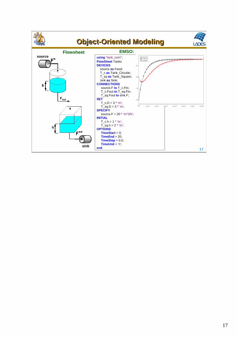
Object-Oriented ModelingObject-Oriented Modeling
using "tank_oom";FlowSheet TanksDEVICES
source as Feed;T_c as Tank_Circular;T_sq as Tank_Square;sink as Sink;
CONNECTIONSsource.F to T_c.Fin;T_c.Fout to T_sq.Fin;T_sq.Fout to sink.F;
SETT_c.D = 3 * ’m’;T_sq.D = 3 * ’m’;
SPECIFYsource.F = 20 * ’m^3/h’;
INITIALT_c.h = 1 * ’m’;T_sq.h = 2 * ’m’;
OPTIONSTimeStart = 0;TimeEnd = 20;TimeStep = 0.5;TimeUnit = ’h’;
end
Fout
Fin
Fout
source
sink
Flowsheet EMSO:

18
18
Object-Oriented ModelingObject-Oriented Modeling
Model switching
Model Tank_Section as Tank_Basic
PARAMETERS
Pi as Real (Default = 3.1416);
Section as Switcher (Valid = ["Circular", "Square"],
Default = "Circular");
EQUATIONS
switch Section
case "Circular":
“Cross section area" A = (Pi * D^2)/4;
case "Square":
“Cross section area" A = D^2;
end
end
using "tank_oom";FlowSheet Tanks2DEVICES
source as Feed;T_c as Tank_Section;T_sq as Tank_Section;sink as Sink;
CONNECTIONSsource.F to T_c.Fin;T_c.Fout to T_sq.Fin;T_sq.Fout to sink.F;
SETT_c.D = 3 * ’m’;T_sq.D = 3 * ’m’;T_c.Section = ”Circular”; T_sq.Section = ”Square”;
SPECIFYsource.F = 20 * ’m^3/h’;
INITIALT_c.h = 1 * ’m’;T_sq.h = 2 * ’m’;
OPTIONSTimeStart = 0;TimeEnd = 20;TimeStep = 0.5;TimeUnit = ’h’;
end

19
19
Object-Oriented ModelingObject-Oriented Modeling
Aggregation
Level Tank
source
sink
P0
P0
P
Tank model
in out
dVF F
dt mass balance:
V A hliquid volume:
0P P g h outlet pressure:
out
PF k
g
valve equation:
Valve model
in outP P P
in outF Fmass balance:
pressure drop:
19

20
20
Object-Oriented ModelingObject-Oriented Modeling
using "types";
Model Tank_Basic
PARAMETERS
D as length (Brief=“Tank hydraulic diameter", Default = 4);
rg as Real (Brief=“rho * g", Unit =’kg/(m*s)^2’, Default = 1e4);
VARIABLES
in Sin as stream (Brief=“Inlet stream");
out Sout as stream (Brief =“Outlet stream");
A as area (Brief=“Cross section area");
V as volume (Brief=“Liquid volume");
h as length (Brief=“Tank level");
valve as Valve (Brief=“Valve model");
CONNECTIONS
Sout to valve.Sin;
EQUATIONS
“Mass balance“ Sin.F – Sout.F = diff(V);
“Liquid volume“ V = A * h;
“Outlet pressure“ Sout.P = Sin.P + rg * h;
end
Tank model with valveusing "types";
Model Valve
PARAMETERS
k as Real (Brief=“Valve constant",
Unit=’m^2.5/h’, Default = 12);
rg as Real (Brief=“rho * g",
Unit =’kg/(m*s)^2’, Default = 1e4);
VARIABLES
in Sin as stream (Brief=“Inlet stream");
out Sout as stream (Brief =“Outlet stream");
DP as press_delta (Brief=“Pressure drop");
EQUATIONS
“Mass balance“ Sin.F = Sout.F;
“Valve equation“ Sout.F = k * sqrt(DP/rg);
“Pressure drop“ DP = Sin.P – Sout.P;
end
Valve model
21
21
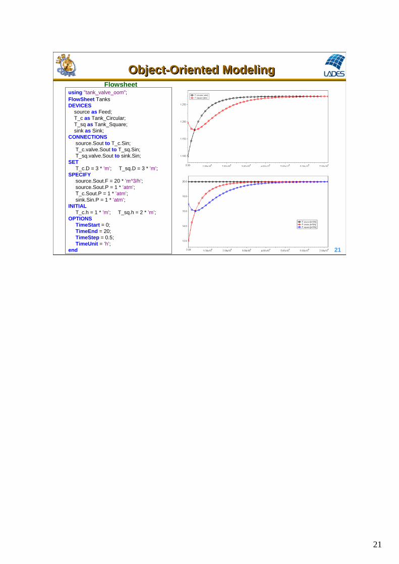
Object-Oriented ModelingObject-Oriented Modeling
using "tank_valve_oom";FlowSheet TanksDEVICES
source as Feed;T_c as Tank_Circular;T_sq as Tank_Square;sink as Sink;
CONNECTIONSsource.Sout to T_c.Sin;T_c.valve.Sout to T_sq.Sin;T_sq.valve.Sout to sink.Sin;
SETT_c.D = 3 * ’m’; T_sq.D = 3 * ’m’;
SPECIFYsource.Sout.F = 20 * ’m^3/h’;source.Sout.P = 1 * ’atm’;T_c.Sout.P = 1 * ’atm’;sink.Sin.P = 1 * ’atm’;
INITIALT_c.h = 1 * ’m’; T_sq.h = 2 * ’m’;
OPTIONSTimeStart = 0;TimeEnd = 20;TimeStep = 0.5;TimeUnit = ’h’;
end
Flowsheet

22
22
Object-Oriented ModelingObject-Oriented Modeling
Creating specialized models by reusing the available library of models
via inheritance and incorporating necessaries characteristics for the new
application.
How to apply for Energy and Sustainability?
Categories
HTPI (Human toxicity potential by ingestion)
HTPE (Human toxicity potential by exposure)
ATP (Aquatic toxicity potential)
TTP (Terrestrial toxicity potential)
GWP (Global warming potential)
ODP (Ozone depletion potential)
PCOP (Photo chemical oxidation potential)
ARP (Acid rain potential)
EP (Eutrophication potential)
Ex: Using the environmental impact factors of the different materials
23
23
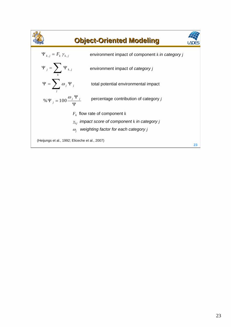
Object-Oriented ModelingObject-Oriented Modeling
,j k j
k
, ,k j k k jF
j j
j
(Heijungs et al., 1992; Eliceche et al., 2007)
Fk flow rate of component k
k,j impact score of component k in category j
j weighting factor for each category j
environment impact of component k in category j
environment impact of category j
total potential environmental impact
% 100 j jj
percentage contribution of category j

24
24
Object-Oriented ModelingObject-Oriented Modeling
Model stream
PARAMETERS
outer NComp as Integer (Brief=“Number of chemical components", Lower = 1);
VARIABLES
F as flow_mol (Brief=“Stream Molar Flow Rate");
T as temperature (Brief =“Stream Temperature");
P as pressure (Brief=“Stream Pressure");
h as enth_mol (Brief=“Stream Enthalpy");
v as fraction (Brief=“Vaporization fraction");
z(NComp) as fraction (Brief=“Stream Molar Fraction");
end
Creating a new stream with environment impact characterization
Model simple_sink
VARIABLES
in Inlet as stream (Brief=“Inlet Stream”);
end
Existing models

25
25
Object-Oriented ModelingObject-Oriented ModelingModel sink_impact as simple_sink
PARAMETERS
outer PP as Plugin (Brief="External Physical Properties", Type="PP");
outer NComp as Integer (Brief=“Number of chemical components", Lower = 1);
Nfactor as Integer (Brief=“Number of categories", Lower=1, Default=9);
w(Nfactor) as fraction (Brief=“Weighting factor");
VARIABLES
psiX(NComp,Nfactor) as frequency (Brief=“Component environment impact");
psiC(Nfactor) as frequency (Brief=“Category environment impact");
psiCp(Nfactor) as percent (Brief=“Category percentage contribution");
psi as frequency (Brief=“Total environment impact");
Fw(NComp) as flow_mass (Brief=“Component Mass Flow Rate");
EQUATIONS
Fw = Inlet.F * Inlet.z * PP.MolecularWeight();
for i in [1:NComp]
psiX(i,:) = Fw(i) * PP.ImpactFactor(i,Nfactor);
end
psiC = sum(psiX);
psi = sum(psiC * w);
psiCp = 100*w*psiC/psi;
end
New stream model

26
26
Object-Oriented ModelingObject-Oriented Modelingusing "streams_impact";using "stage_separators/flash";FlowSheet flash_impactPARAMETERS
PP as Plugin (Brief="Physical Properties", Type="PP",Components = ["hydrogen", "methane", "benzene", "toluene", "biphenyl", "water"],LiquidModel = "PR", VapourModel = "PR");
NComp as Integer;VARIABLES
Q as energy_source (Brief="Heat supplied");SET
NComp = PP.NumberOfComponents;DEVICES
fl as flash;s1 as source;top as sink_impact;bot as sink_impact;
CONNECTIONSs1.Outlet to fl.Inlet;Q.OutletQ to fl.InletQ;fl.OutletV to top.Inlet;fl.OutletL to bot.Inlet;
...
A simple examplefile ex_impact.mso

27
27
Object-Oriented ModelingObject-Oriented Modeling
0 1 2 3 4 5 6 7 80
200
400
time (h)
Tot
al im
pact
(to
p)
0 1 2 3 4 5 6 7 85500
6000
6500
Tot
al im
pact
(bo
ttom
)
Response of the potential environment impact for a +20% step change in the feed flow rate at time = 4h.
Impact category % Contribution (top)
% Contribution (bottom)
Human toxicity by ingestion 7.58 6.57 Human toxicity by exposure 0.58 5.23 Aquatic toxicity 7.58 6.57 Terrestrial toxicity 2.71 7.91 Global warming 0.34 0.110-3 Ozone depletion 0.00 0.00 Photo chemical oxidation 81.21 73.72 Acid rain 0.00 0.00 Eutrophication 0.00 0.00
Category contribution for the potential environment impact at the final time

28
28
Object-Oriented ModelingObject-Oriented Modeling
0 1 2 3 4 5 6 7 8100
200
300
400
500
time (h)
Tot
al im
pact
(to
p)
0 1 2 3 4 5 6 7 84500
5000
5500
6000
6500
Tot
al im
pact
(bo
ttom
)
Results with pressure and level controllers
0 1 2 3 4 5 6 7 80
5
10
Pre
ssur
e (a
tm)
time (h)0 1 2 3 4 5 6 7 8
0
100
200
Vap
or flow rat
e (k
mol/h
)
0 1 2 3 4 5 6 7 80.9
1
1.1
Leve
l (m
)
time (h)0 1 2 3 4 5 6 7 8
300
350
400
Liqu
id flo
w rat
e (k
mol
/h)
Disturbances:
Pressure set-point at time = 2h
5 atm 8 atm
Temperature and feed flow rate at time = 4h
340 K 360 K
500 kmol/h 450 kmol/h

29
29
3. Modeling Workshop3. Modeling Workshop
EMSOEMSO stands for “Environment for MModeling, SSimulation, and OOptimization”
Development started in 2001 (by Rafael P. Soares), written in C++ language
Available in Windows and Linux
Models are written in an object-oriented modeling language
Equation-oriented simulator and optimizer
Computationally efficient for dynamic and steady-state simulations
Continuous improvements through ALSOC project:
http://www.enq.ufrgs.br/alsoc
Introducing EMSO

30
30

31
31
EMSO Key FeaturesEMSO Key Features
Open source library of models
Object-oriented modeling
Built-in automatic and symbolic differentiation
Automatic checking and conversion of units of measurement
Solve high-index problem
Perform consistency analysis (DoF, DDoF, initial condition)
Integrated Graphical User Interface (GUI)
Building blocks to create flowsheets
Discrete (state and time) event handling
Multitask for concurrent and real-time simulations
Modular architecture and support to sparse algebra
Multiplatform: win32 and posix
Interface with user code written in C/C++ or Fortran
Automatic documentation of models using hypertexts and LaTeX

32
32
Steady-state simulations
Dynamic simulations
Steady-state optimizations (NLP, MINLP)
Steady-state parameter estimations
Dynamic parameter estimations
Steady-state data reconciliations
Process follow-up and inferences with OPC communication
Build bifurcation diagrams (interface with AUTO for DAEs)
Dynamic simulations with SIMULINK (interface with MATLAB)
Add new solvers (DAE, NLA, NLP)
Add external routines using the Plugins resource
What can I do with EMSO?What can I do with EMSO?

33
33
Thermodynamic andPhysical Properties – Plugin
Thermodynamic andPhysical Properties – Plugin
Data bank with about 2000 pure compounds
Mixture properties calculation

34
34
How can I install EMSO?How can I install EMSO?
Download EMSO and
VRTherm packages from
http://www.enq.ufrgs.br/alsoc
Run the setup programs
Run EMSO
Add the physical properties
package using the Config
Plugins option in the menu
Select an example and run it

35
35
To use a plugplug--in thein the user needsto register it through the menu
ConfigConfig PluginsPlugins
WindowsWindows plugplug--in is ain is a DLL file, and LinuxLinux plug-in is a SO file
Configuring Plugin– VRTherm package: vrpp –
Configuring Plugin– VRTherm package: vrpp –
36
36
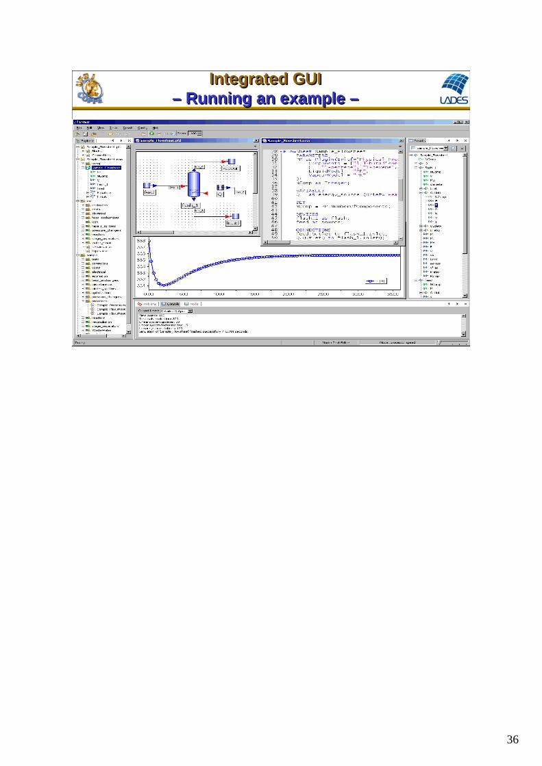
Integrated GUI– Running an example –
Integrated GUI– Running an example –

37
37
Modeling workshopModeling workshop
Model equations
in out
dVF F
dt mass balance:
outF k hvalve equation:
Fin
Fout
h
A = h (D h)
2
2 3
D hV h
liquid volume:
V A h
Fin
Fin
Fin
Fout
Fout
Fout

38
38
Flowsheet
Modeling workshopModeling workshop
Fin
Fout
source
Fout
Fout
h
Fout
sink
= 20 m3/h
D = 3 m
h(0) = 1 m
D = 3 m
h(0) = 2 m
D = 3 m
h(0) = 2.5 m

3939
39
Basic Elements in Modeling
1. Process description and problem definition
2. Fundamental laws: theory and application
3. Simplifying assumptions
4. Mathematical model
5. Consistency analysis
6. Desired solution
7. Computation
8. Solution and validation
Model definition
Model building
Model validation
Remarks about ModelingRemarks about Modeling

4040
40
1. Process Description and Problem Definition1. Process Description and Problem Definition
• Process Description– Process objectives– Process flowsheet– Process operation
• unit operations and control
• Problem Definition– Simulation objectives– Simulation applications

4141
41
Process DescriptionProcess Description
Example: level tank
h
Fout
Fin
V
A liquid flows in and out of a tank due to gravitational forces.
We wish to analyze the volume, height and flowrate variations in
the tank (system response) as function of feed disturbances.

4242
42
2. Fundamental Laws: Theory and Applications2. Fundamental Laws: Theory and Applications
t
v ( . )
advection pressure forces viscous forces gravitational forces
( )[ . ] [ . ]
vv v P g
t
2 2
advection conduction gravit. forces work pressure forces work viscous forces work
1 1ˆ ˆ. ( . ) . ( . ) ( .[ . ])2 2
U v v U v q g v P v vt
- mass conservation
- momentum conservation
- energy conservation
• Bases to be used in the modeling

4343
43
3. Simplifying Assumptions3. Simplifying Assumptions
- constant specific mass
- isothermal
- perfect mixture
- outF k h
• Establish the assumptions and simplifications
• Define the model limitations

4444
44
4. Mathematical Model4. Mathematical Model
• Data mining for simulation– Collect data and information of the studied system– Identify the engineering unit of measurements– Specify operating procedures– Specify the operating regions of the variables
• Memory of Calculation– Mathematical model– Define unit of measurements of variables and parameters– Define and specify free variables– Define and determine values of parameters– Define and establish initial conditions

4545
45
4. Mathematical Model4. Mathematical Model
First Principles
Models
Conservation laws
XV
Fμ
dt
dX
Fdt
dV
)T(TρVC
UAT)(T
V
F
dt
dTc
pe
Empirical Models
Neural Nets
Fuzzy Logic
Parametric
e(t)D(q)
C(q)u(t)
F(q)
B(q)y(t)A(q)
Hybrid Models

4646
46
• Build process equipment models– Identify and create abstract and concrete models– Declare variables and parameters– Write model equations– Compose the equipment model via inheritance and aggregation
• Build process flowsheet– Declare flowsheet devices– Define process connections– Set process parameters values– Specify process free variables– Establish initial conditions– Establish simulation options
Mathematical ModelMathematical Model
In the simulator

47
47
Fin
Fin
Fin
Fout
Fout
Fout
in out
dVF F
dt mass balance:
outF k hvalve equation:
V A hliquid volume:
Mathematical ModelMathematical Model
(1)
(2)
(3)
(4)

4848
48
5. Consistency Analysis5. Consistency Analysis
• Model consistency analysis for unit of measurements (UOM)
• Degree of freedom analysis
• Dynamic degree of freedom analysis
variable UOM
Fin, Fout m3 h-1
V m3
A m2
h, D m
k m2.5 h-1
t h
equations
(1): [m3 h-1] – [m3 h-1] = [m3] / [h]
(2): [m3 h-1] = [m2.5 h-1] ([h])0.5
(3): [m3] = [m2] [m]
(4): [m2] = ([m])2

4949
49
variables: Fin, Fout, V, A, h, D, k, t 8
constants: k, D 2
specifications: t 1
driving forces: Fin 1
unknown variables: V, h, A, Fout 4
equations: 4
Degree of Freedom = variables – constants – specification – driving forces –
equations = unknown variables – equations = 8 – 2 – 1 – 1 – 4 = 0
Dynamic Degree of freedom (index < 2) = differential equations = 1
Needs 1 initial condition: h(0) 1
Consistency AnalysisConsistency Analysis

5050
50
For the given example and initial condition (h0 or V0), we wish to analyze h(Fin), V(Fin) and Fout(Fin).
6. Desired Solution6. Desired Solution
• Plan case studies• Define:
– Objectives of the study– Problems to be solved– Evaluation criteria

51
51
7. Computation7. Computation
• Define the desired accuracy
• Specify the simulation time and reporting interval
• Verify the necessity of specialized solvers (high-index problems)

5252
52
• Analyze simulation results
• Analyze state variables dynamics
• Test model fitting with plant data
– Compare simulation x plant
hexp
hcalc
8. Solution and Validation8. Solution and Validation

5353
53
• Check output sensitivity to input disturbances
• Carry out parametric sensitivity analysis
• Analyze output data with statistical techniques
• Verify results coherence
• Document obtained results
Solution and ValidationSolution and Validation

5454
54
• Start with a simple model and gradually increase complexity when necessary;
• The model should have sufficient details to capture the essence of the studied system;
• It is not necessary to reproduce each element of the system;
• Models with excessive details are expensive, difficult to implement and to solve;
• Interact with people that operate the equipment;
• Deeply understand the process behavior.
CommentsComments

55
55
In Equation-Oriented (EO) simulators a model has:
• A set of model parameters (reaction order, valve constant, etc.)
• A set of variables (temperatures, pressures, flow rates, etc.)
• A set of equations (algebraic and differential) relating the variables
Problems in model building:
• Number of equations and variables do not match
• Equations of the model are inconsistent (linear dependence, etc.)
• The number of initial conditions and DDoF do not match
4. Dynamic Degree of Freedom4. Dynamic Degree of Freedom

56
56
Check Units of measurement
Structural non-singularity
Consistent initial conditions
Degree of Freedom (DoF)
= 0 (for simulation) > 0 (for optimization)
Dynamic Degree of Freedom (DDoF)
= number of given initial conditions
Dynamic Degree of Freedom– Consistency Analysis –
Dynamic Degree of Freedom– Consistency Analysis –

57
57
Dynamic Degree of Freedom– General Concept –
Dynamic Degree of Freedom– General Concept –
Given a system of DAE: F(t, y, y’) = 0
The Dynamic Degree of Freedom (DDoF) is the number of variables in
y(t0) that can be assigned arbitrarily to compute a set of consistent initial
conditions {y(t0), y’(t0)} of the DAE system. Is the true number of states of
the system (or the system order of the DAE). Is the number of initial
conditions that must be given.
For low-index DAE system (index 0 and 1) the DDoF is equal to the
number of differential equations.
For high-index DAE system (index > 1) the DDoF is equal to the number
of differential variables minus the number of hidden constraints.

5858
58
1 2 0x x
1 ( )x u tExample: differentiating
twice in t 2 ( )x u t 1 2x x
= 2
Differential index (): Is the minimum number of times the DAE system
F(t,x,x’,u) = 0 needs to be differentiated with respect to t to be transformed in an
explicit ODE system in terms of x’.
If the resolution of a DAE system presents difficulties for initializing and/or
presents error propagation in the numerical integration, then this system has an
index problem, this problem may occur in DAE systems with > 1.
Dynamic Degree of Freedom– DAE System Characterization –Dynamic Degree of Freedom– DAE System Characterization –

5959
59
Substituting the first differentiation: 1 ( )x u t
2 ( )x u tin the first equation, results in:
In the initial time: 1(0) (0)x u
2 (0) (0)x u
1(0) (0)x u
2 (0) (0)x u
Therefore, there is no dynamic degree of freedom, i.e., the system did not accept any arbitrary initial conditions.
Dynamic Degree of Freedom– Consistent Initial Conditions –Dynamic Degree of Freedom– Consistent Initial Conditions –

6060
60
Consistent initial conditions: The vectors x(t0) and x’(t0) form a consistent initial condition of the DAE system F(t,x,x’,u) = 0 at t0 if they satisfy the extended system at t0.
The most difficult step for solving DAE systems is the determination of consistent initial conditions.
During the differentiation process to reduce the index of a DAE system to zero, hidden constraints may arise. The original system augmented by the set of the hidden equations is called extended system.
1 2 0x x
1 ( )x u t 2 ( )x u t 2 ( )x u tExtended system of
the example:
Dynamic Degree of Freedom– Consistent Initial Conditions –Dynamic Degree of Freedom– Consistent Initial Conditions –

61
61
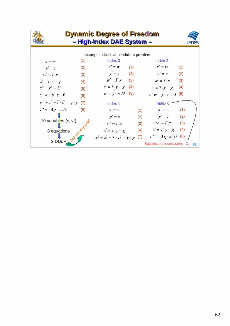
Example: classical pendulum problemInconsistent initial condition:
L
( , , ) 0F t y y (0, (0), (0)) 0F y y
(1)
(2)
(3)
(4)
(5)
Differentiating (5) and using (1) and (2): 0x w y z (0) (0) (0) (0) 0x w y z
Differentiating (6) and using (1)–(5):
(6)
(7)
Differentiating (7) and using (2), (3), (4), (6):
2 2 2w z T L g y 2 2 2(0) (0) (0) (0)w z T L g y
2' 3 /T g z L (8) 2'(0) 3 (0) /T g z L
OK!
NO
T OK
!
Hidden constraints:
Dynamic Degree of Freedom– High-Index DAE System –
Dynamic Degree of Freedom– High-Index DAE System –
62
62
Example: classical pendulum problem(1)
(2)
(3)
(4)
(5)
(6)
(7)
(8)
10 variables (y, y´)
8 equations
2 DDoF
(1)
(2)
(3)
(4)
(5)
(1)
(2)
(3)
(4)
(6)
(1)
(2)
(3)
(4)
(7)
(1)
(2)
(3)
(4)
(8)
Index 3 Index 2
Index 1 Index 0
Satisfies the inconsistent I.C.
But n
ot a
ny p
air!
Dynamic Degree of Freedom– High-Index DAE System –
Dynamic Degree of Freedom– High-Index DAE System –

63
63
Three general approaches:
1) Manually modify the model to obtain a lower index equivalent model
2) Integration by specifically designed high-index solvers (e.g., PSIDE, MEBDF, DASSLC)
EMSO: Integration = “original”
3) Apply automatic index reduction algorithms
EMSO: Integration = “index0”
or EMSO: Integration = “index1”
Dynamic Degree of Freedom– High-Index DAE: solution –
Dynamic Degree of Freedom– High-Index DAE: solution –

64
64
Dynamic Degree of Freedom– High-Index DAE: modeling –
Dynamic Degree of Freedom– High-Index DAE: modeling –

65
65
Dynamic Degree of Freedom– High-Index DAE: consistency analysis –
Dynamic Degree of Freedom– High-Index DAE: consistency analysis –

66
66
x
index-0 solver vs index-3 solver Drift-off effect
L = 0.9 m , g = 9.8 m/s2 I.C.: x(0) = 0.9 m and w(0) = 0
Dynamic Degree of Freedom– High-Index DAE: simulation –
Dynamic Degree of Freedom– High-Index DAE: simulation –
Error propagation

67
67
Batch distillation column with optimal composition control (index 3) (Logsdson and Biegler, 1993)
1
13579
10
R
Dynamic Degree of Freedom– Workshop –
Dynamic Degree of Freedom– Workshop –
Batch Distillation

68
68
• negligible vapor holdup (no dynamics in vapor phase);
• thermodynamic equilibrium (ideal stage);
• no droplet drag in vapor stream;
• ideal gas and liquid;
• constant liquid holdup in each tray;
• perfect mixture in both phases;
• constant pressure;
• optimal control of distillate composition;
• vapor pressure described by Antoine equation.
Model assumptions
Dynamic Degree of Freedom– Workshop –
Dynamic Degree of Freedom– Workshop –

69
69
Mass balance in the reboilerOverall:
Component:
(2)
(1)
(3)
0
1
dH V
dt R
00 0 1 0
0
1,..., 11
jj j j jdx V R
x y x x j ncdt H R
Mass balance in each tray component:
1 1
1,...,
1,..., 11
jj j j ji
i i i ii
i npdx V Ry y x x
j ncdt H R
Batch distillation modeling
Dynamic Degree of Freedom– Workshop –
Dynamic Degree of Freedom– Workshop –

70
70
Mass balance in the condenser Component:
(5)
(4)
(7)
Molar fractions
11
1
1,..., 1j
np j jnp np
np
dx Vy x j nc
dt H
1
1 0,..., 1nc
ji
j
y i np
1
1 0,..., 1nc
ji
j
x i np
(6)
0,..., 1exp
1,...,jj j
i ref j ii j
B i npy P P A x
j ncT C
Thermodynamic equilibrium
Dynamic Degree of Freedom– Workshop –
Dynamic Degree of Freedom– Workshop –
Batch distillation modeling

71
71
variable units of measurement
Hi kmol
V kmol/s
t s
R –
xij, yi
j kmol/kmol
P, Pref kPa
Ti K
Aj –
Bj K
Cj K
Consistency analysis
Dynamic Degree of Freedom– Workshop –
Dynamic Degree of Freedom– Workshop –

72
72
variables: Hi, V, t, R, xij, yi
j, P, Pref, Ti, Aj, Bj, Cj 5 + 2 (np+2)(nc+1) + 3 ncconstants: Pref, Aj, Bj, Cj 3 nc + 1specifications: t,V, P, Hi, x1
np+1 5 + np (i = 1,...,np+1)driving forces: 0unknown variables: H0, R, xi
j, yij, Ti 3 + 2 (np+2) nc + np
equations: 3 + 2 (np+2) nc + np
Degree of Freedom = variables – constants – specifications – driving forces –equations = unknown variables – equations = 0
Dynamic Degree of Freedom (index = 3) = np (nc – 1) + 2 (nc – 2)
Needs np (nc – 1) + 2 (nc – 2) initial conditions.
Para nc = 2: H0(0), R(0), x01(0), Ti(0) (i = 2,...,np–2)
Consistency analysis
Dynamic Degree of Freedom– Workshop –
Dynamic Degree of Freedom– Workshop –

73
73
Dynamic Degree of Freedom– Workshop –
Dynamic Degree of Freedom– Workshop –
EMSO
73

74
74
Dynamic Degree of Freedom– Workshop –
Dynamic Degree of Freedom– Workshop –
EMSO
74

75
75
time
Dynamic Degree of Freedom– Workshop –
Dynamic Degree of Freedom– Workshop –
EMSO
75

76
76
• Reports system singularity:
Dynamic Degree of Freedom– Workshop –
Dynamic Degree of Freedom– Workshop –
AspenDynamics

77
77
• Detects a high-index problem and gives the following error message:
Dynamic Degree of Freedom– Workshop –
Dynamic Degree of Freedom– Workshop –
gPROMS
7878
78
- Multiplicity of steady states
- Linearization
- System stability
- Complex dynamic behaviors (limit cycles, strange attractors)
- Parametric sensitivity and input sensitivity
5. System Analysis5. System Analysis

79
79
Non-isothermal CSTR
Fe , CAf , CBf , Tf
Fwe , Twe
Fws , Tw
Fs , CA , CB , T
V , T
A kB
Multiplicity of Steady StatesMultiplicity of Steady States

80
80
In a non-isothermal continuous stirred tank reactor, with diameter of 3.2 m
and level control, pure reactant is fed at 300 K and 3.5 m3/h with concentration
of 300 kmol/m3. A first order reaction occur in the reactor, with frequency factor
of 89 s-1 and activation energy of 6 x 10⁴ kJ/kmol, releasing 7000 kJ/kmol of
reaction heat. The reactor has a jacket to control the reactor temperature, with
constant overall heat transfer coefficient of 300 kJ/(h.m2.K). Assume constant
density of 1000 kg/m3 and constant specific heat of 4 kJ/(kg.K) in the reaction
medium. The fully-open output linear valve has a constant of 2.7 m2.5/h.
Process description
Multiplicity of Steady StatesMultiplicity of Steady States

81
81
• perfect mixture in the reactor and jacket;
• negligible shaft work;
• (-rA) = k CA;
• constant density;
• constant overall heat transfer coefficient;
• constant specific heat;
• incompressible fluids;
• negligible heat loss to surroundings;
• (internal energy) (enthalpy);
• negligible variation of potential and kinetic energies;
• constant volume in the jacket;
• thin metallic wall with negligible heat capacity.
Model assumptions
Multiplicity of Steady StatesMultiplicity of Steady States

82
82
dt
dVFF
dt
Vdsef
)(
se FFdt
dV
)( AAsfAeA
AA rVCFCFdt
dVC
dt
dCV
dt
VCd
Mass balance in the reactorOverall:
Component:
(2)VrCCFdt
dCV AAfAe
A )()(
(1)
eF
V (3)
CSTR modeling
Multiplicity of Steady StatesMultiplicity of Steady States

83
83
(4)
2 2
ˆˆ ˆ ˆ ˆ ˆ ˆ2 2f s
e f f f f s s r s
v vdV U K F U P V gz F U PV gz q q w
dt
ˆ ˆ ˆH U PV
ˆ ˆ( ) ˆ ˆ ˆe f s r
d VH dH dVV H F H F H q q
dt dt dt
Energy balance in the reactor:
where
ˆˆ ˆ( )e f r
dHV F H H q q
dt
qqTTCpFdt
dTVCp rfe )(
CSTR modeling
Multiplicity of Steady StatesMultiplicity of Steady States

84
84
(5)where
qr = (-Hr) V (-rA)
k = k0 exp(–E/RT)
(-rA) = k CA
V = A h
Fs = x Cv h
Tw = f(T)
(7)
(6)
(8)
(10)
(12)
Temperature control (14)
At = A + D h (11)
q = U At (T – Tw)
A = D2/4 (9)
x = f(h) Level control (13)
CSTR modeling
Multiplicity of Steady StatesMultiplicity of Steady States

85
85
variable units of measurement
Fe, Fs m3 s-1
V m3
t, s
CA, CAf kmol m-3
rA kmol m-3 s-1
kg m-3
Cp kJ kg-1 K-1
T, Tf, Tw K
qr, q kJ s-1
U kJ m-2 K-1 s-1
At, A m2
h, D m
Cv m2.5 h-1
x –
Hr, E kJ kmol-1
R kJ kmol-1 K-1
k, k0 s-1
Consistency analysis
Multiplicity of Steady StatesMultiplicity of Steady States

86
86
variables: Fe, Fs, V, t, CA, CAf, rA, , Cp, T, Tf, Tw, qr, q, U, At, A, h, D, Cv, x, Hr, E, R, k, k0, 27constants: , Cp, U, D, Cv, Hr, E, R, k0 9specifications: t 1driving forces: Fe, Tf, CAf 3unknown variables: Fs, V, CA, rA, T, Tw, qr, q, A, At, h, x, k, 14equations: 14
Degree of Freedom = variables – constants – specifications – driving forces –equations = unknown variables – equations = 27 – 9 – 1 – 3 – 14 = 0
Dynamic Degree of Freedom (index < 2) = differential equations = 3
Needs 3 initial condition: h(0), CA(0), T(0) 3
Consistency analysis
Multiplicity of Steady StatesMultiplicity of Steady States

87
87
Running EMSO
Open MSO file
Multiplicity of Steady StatesMultiplicity of Steady States

88
88
Consistency Analysis
Results

89
89

9090
90
The CSTR example at the steady state satisfy:
0
0
( )1( ) ( )
1
E
RTr Aft
f w EP RT
P
H k e CU AT T T T
V CC k e
e
V
F
01
AfA E
RT
CC
k e
Multiplicity of Steady StatesMultiplicity of Steady States

9191
91
Rewriting the energy balance:
( ) ( )R GQ T Q T0
0
( )( )
1
E
RTr Af
G E
RTP
H k e CQ T
C k e
Q T a T bR ( )
aU A
V Ct
P
1
f t w
P
T U A Tb
V C
T
Q
QG
QR3QR2QR1
1 2
3
4
5
GR dQdQ
dT dT
stable:
GR dQdQ
dT dT
unstable:
Multiplicity of Steady StatesMultiplicity of Steady States

9292
92
( , )dx
F t xdt
( ) 0F x
1( 1) ( ) ( ) ( )( ) ( ) , 0,1, 2,k k m kx x J x F x k Newton-Raphson:
( )( ) ( )
( )k
k iij
j
F xJ x
x
and 0 1m k
Path FollowingPath Following
Homotopic Continuation: ( ; ) (1 ) ( ) ( ) 0 , 0 1H x p p F x p G x p
(0) (0)( ) ( ) ( )G x J x x x (0)( ) ( ) ( )G x F x F x
affine homotopy
Newton homotopy
Multiples solutions can be obtained by continuously varying the parameter p
Multiplicity of Steady StatesMultiplicity of Steady States

9393
93
Parametric Continuation: [ ( ); ( )] 0F x s p s where s is some parameterization, e.g., path arc length
( ) ( ) 0 , eF F dx dp
x s p s x px p ds ds
F FDF
x p
Frechet derivative
a point (xo, po) is:
( , )o oF x p
x
- Regular if is non-singular
( , )o oF x p
x
- Turning point if is singular and DF has rank = n
( , )o oF x p
x
- Bifurcation if is singular and DF has rank < n
reparameterization
Path FollowingPath FollowingMultiplicity of Steady StatesMultiplicity of Steady States
9494
94
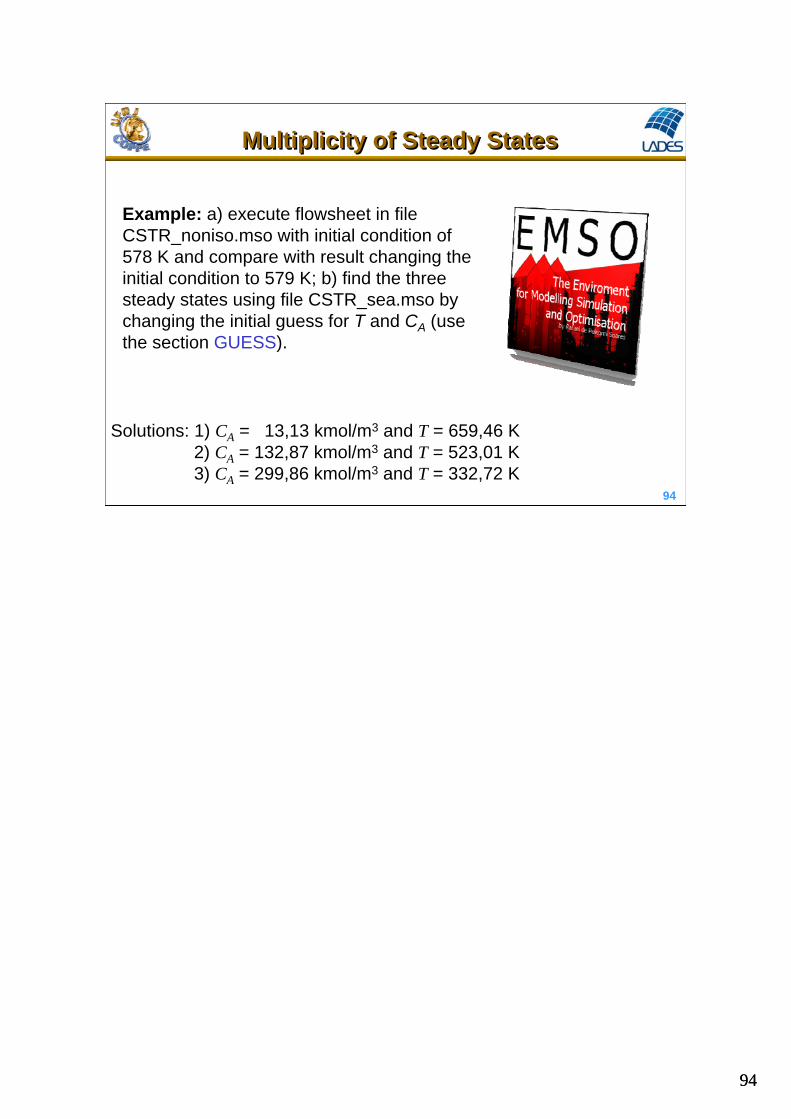
Solutions: 1) CA = 13,13 kmol/m3 and T = 659,46 K2) CA = 132,87 kmol/m3 and T = 523,01 K3) CA = 299,86 kmol/m3 and T = 332,72 K
Example: a) execute flowsheet in file CSTR_noniso.mso with initial condition of 578 K and compare with result changing the initial condition to 579 K; b) find the three steady states using file CSTR_sea.mso by changing the initial guess for T and CA (use the section GUESS).
Multiplicity of Steady StatesMultiplicity of Steady States

95
95
LinearizationLinearization
Generate linearized model at given operating point.
Implicit DAE:
Considering the specification as input, u(t), (SPECIFY section in EMSO):
And identifying the algebraic variables as y(t):
( ,́ , , , ) 0F x x y u t
( ,́ , ) 0F x x t
ˆ ˆ( ,́ , , ) 0F x x u t

96
96
Differentiating F:
and extracting:
The partition:
Define the linearized system:
Linearization
´ 0x x y uF dx F dx F dy F du
1
x y x u
dx dxF F F F
dy du
1
x y x u
A BF F F F
C D
'x A x B u
y C x Du
(index < 2)

97
97
Test example for a linear model: exact solution!
Linearization
98
98
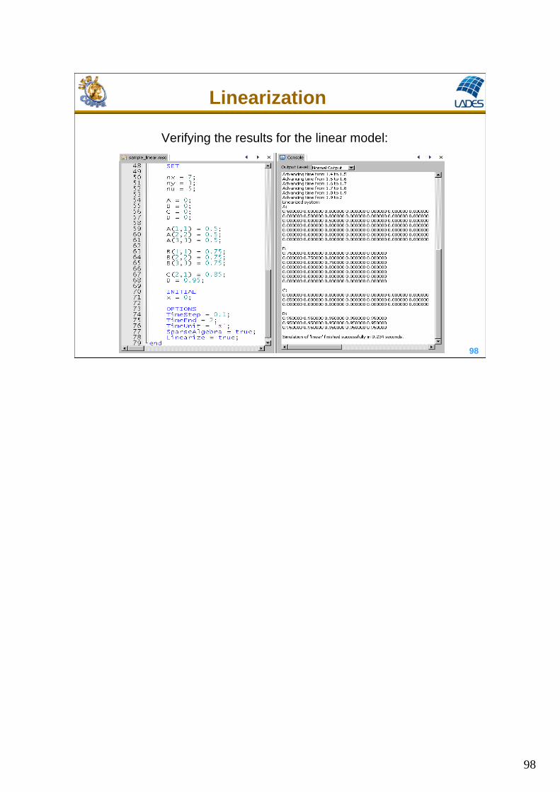
Verifying the results for the linear model:
Linearization

9999
99
Example: execute the flowsheet in file CSTR_linearize.mso with the option Linearize = true and evaluate the characteristic values of the Jacobianmatrix (matrix A). Repeat the example with the value of Cp 10 times smaller, i.e., 0.4 kJ / (kg K). Compare the ratio between the greater and the smaller characteristic values in module.
Non-isothermal CSTR: linearizationNon-isothermal CSTR: linearization

100100
100
Stability AnalysisStability Analysis
)(tx
( )dx
F xdt
0 0( ) ( )x t y t ( ) ( )x t y t
Liapunov Stability: is stable (or Liapunov stable) if, given > 0, there exists a = () > 0, such that, for any other solution, y(t), of
satisfying , then for t > t0.

101101
101
Stability AnalysisStability Analysis
)(tx
0 0( ) ( )x t y t b Asymptotic Stability: is asymptotic stable if Liapunov stable and there exists a constant b > 0 such that, if then 0)()(lim
tytx
t
( ) ( ) ( )y t x t x t Defining deviation variables:
2[ ( )]( ) ( ( ))
dx F x tF x F x t y O y
dt x
( ( ) )dx dx dy
F x t ydt dt dt
Expanding in Taylor series:
Linearization: [ ( )] ( )dy
J x t y A t ydt

102102
102
( )x tFor an equilibrium point = x*, the stability is characterized by the characteristics values of the Jacobian matrix J(x*) = A:
x* is a hyperbolic point if none characteristics values of J(x*) has zero real part.
x* is a center if the characteristics values are pure imaginary. Fixed point non-hyperbolic.
x* is a saddle point, unstable, if some characteristics values have real part > 0 and the remaining have real part < 0.
x* is stable or attractor or sink point if all characteristics values have real part < 0.
x* is unstable or repulsive or source point if at least one characteristic value have real part > 0.
Stability AnalysisStability Analysis

103103
103
For a second-order linear system:2det( ) ( ) det( ) 0A I tr A A
2( ) ( ) 4det( )
2
tr A tr A A
Stability AnalysisStability Analysis

104104
104
0 0( ) , (0)E
RTeAA A A A Af
FdCC C k e C C C
dt V
00
( ) ( )( ) , (0)
E
R Te r A t w
fp p
F H k e C UA T TdTT T T T
dt V C V C
Considering the CSTR example with constant volume:
0 02
0 02
( , )( ) ( )
E E
R T RTeA
E EAR T R T
r e r A t
p p p
F Ek e k e C
V R TJ C T
H k e F H k e C UAE
C V R T C V C
Stability AnalysisStability Analysis

105105
105
3 4
3 4
1.6458 10 3.4282 10(13.13, 659.46)
2.7542 10 4.8934 10J
4 4
4 4
1.6260 10 3.1753 10(132.87, 523.01)
1.5852 10 4.4509 10J
5 7
8 4
7.2050 10 6.6220 10(299.86, 332.72)
5.9285 10 1.0944 10J
5
4
7.2051 10
1.0944 10
5
4
6.3659 10
3.4614 10
3
4
1.0205 10
1.3604 10
2) Saddle Point, unstable
1) Stable node
3) Stable Node
Stability AnalysisStability Analysis

106106
1060 50 100 150 200 250 300 350
300
350
400
450
500
550
600
650
700
750
800
CA
T
file: CSTR_nla/traj_cstr.m
Stability AnalysisStability Analysis
107107
107
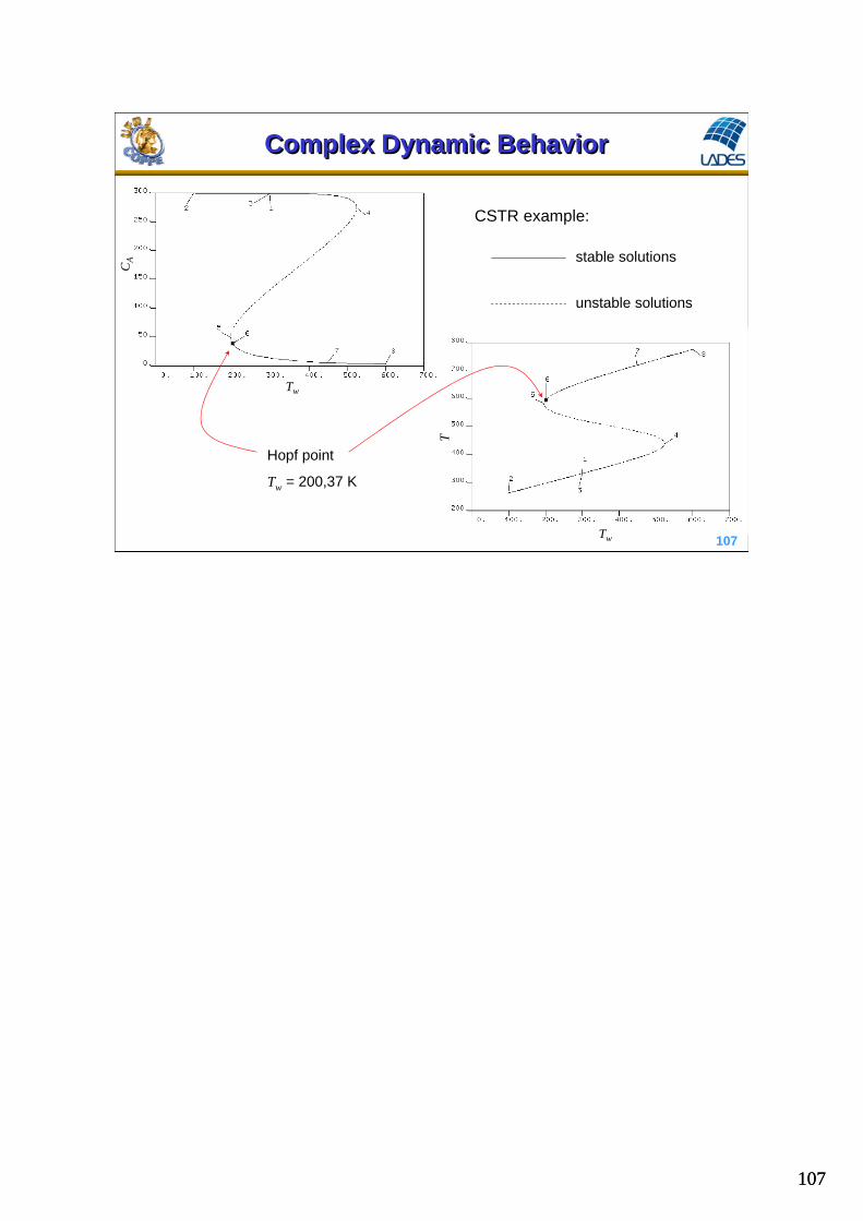
Complex Dynamic BehaviorComplex Dynamic Behavior
Tw
Tw
CA
THopf point
Tw = 200,37 K
unstable solutions
stable solutions
CSTR example:

108108
108
t (h)
t (h)
unstable limit cycle
A limit cycle is stable if all characteristics values of exp(J p) (Floquet multipliers) are inside the unitary cycle, where J is the Jacobian matrix in the cycle, p = 2 / is the oscillation period and = |Hopf|.
file: CSTR_auto/cstr_bif.mso
Complex Dynamic BehaviorComplex Dynamic Behavior

109
109
Interface EMSO-AUTOInterface EMSO-AUTO
parameters
Equation system
Jacobian matrix
First steady-state solution

110110
110
Interface EMSO-AUTOInterface EMSO-AUTO
21 ( )1 11 x tdx t
x t p x t edt
222 13 14 1 x tdx t
x t p x t edt
2 2
2 2
1
1
1 (1 )( )
14 3 14 (1 )
x x
x x
p e p x eJ x
p e p x e
p = 0: x* = (0, 0) (J) = (-1, -3)

111111
111
Interface EMSO-AUTOInterface EMSO-AUTO
0 0.2 0.4 0.6 0.8 1 1.2 1.4 1.6 1.8 20
1
2
3
4
5
6
7
8
9
10
x1
x 2
0 0.02 0.04 0.06 0.08 0.1 0.12 0.14 0.16 0.18 0.20
0.1
0.2
0.3
0.4
0.5
0.6
0.7
0.8
0.9
1
x1
x 2
0.134 0.136 0.138 0.14 0.142 0.144 0.146 0.148
0.63
0.64
0.65
0.66
0.67
0.68
0.69
x1
x 2
Complex eigenvalues with negative real part - stable focusp = 0.085 = -1.095 0.565 i
0.06361 < p < 0.0889
Repeated real negatives eigenvalues – stable node (star) = [-1.4372, -1.4372]
p = 0.06361
Real negatives eigenvalues –stable nodep = 0.05 = [-1.13, -2.06]
p < 0.06361
Phase planeEigenvaluesParameter p

112112
112
Interface EMSO-AUTOInterface EMSO-AUTO
0 0.2 0.4 0.6 0.8 1 1.2 1.4 1.6 1.8 20
1
2
3
4
5
6
7
8
9
10
x1
x 2
0 0.1 0.2 0.3 0.4 0.5 0.6 0.7 0.8 0.9 10
1
2
3
4
5
6
7
x1
x 2
0 0.1 0.2 0.3 0.4 0.5 0.6 0.7 0.8 0.9 10
1
2
3
4
5
6
7
x1
x 2
One stable solution (focus) and two unstable (saddle and focus)p = 0.10 = -0.652 0.651 i = [-0.439, 1.953] = 1.431 1.851 i
0.0933 < p < 0.10574at p = 0.105738931 the first point goes from stable focus to stable node: = [-0.055, -0.046]
One stable solution (focus) and two unstable (saddle and node)p = 0.09 = -0.982 0.614 i = [-0.213, 3.332] = [0.364, 3.151]
0.0889 < p < 0.0933
Turning point (fold): One stable solution (focus) and other unstable (node). (point 3 in figure below) = -1.009 0.605 i = [0, 3.432]
p = 0,0889unstable node gives rise to two points: unstable node and saddle point p > 0.0889

113113
113
Interface EMSO-AUTOInterface EMSO-AUTO
0 0.1 0.2 0.3 0.4 0.5 0.6 0.7 0.8 0.9 10
1
2
3
4
5
6
7
x1
x 2
0 2 4 6 8 10 12 14 16 18 200
2
4
6
8
10
12
t
x
0 0.2 0.4 0.6 0.8 1 1.2 1.4 1.6 1.8 20
2
4
6
8
10
12
x1
x 2
0.8 0.82 0.84 0.86 0.88 0.9 0.92 0.94 0.96 0.98 13
3.5
4
4.5
5
5.5
6
x
2
Hopf bifurcation: pure imaginary eigenvalues. (point 4 in figure below) = 4.008 i
p = 0.1309
One unstable solution (focus) and one stable limit cyclep = 0.12 = 0.528 3.487 i
0.10574 < p < 0.1309
Turning point (fold): One stable solution (node), other unstable (focus), and one sable limit cycle. (point 2 in figure below) = [-0.097, 0] = 1.186 2.478 i
p = 0.10574the stable node gives rise to two points: stable node and saddle forp < 0.10574
114114
114
Interface EMSO-AUTOInterface EMSO-AUTO
0.8 0.82 0.84 0.86 0.88 0.9 0.92 0.94 0.96 0.98 13
3.5
4
4.5
5
5.5
6
x1
x 2
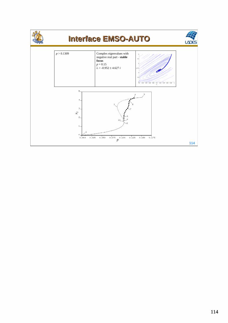
Complex eigenvalues with negative real part - stable focusp = 0.15 = -0.952 4.627 i
p > 0.1309
p
x 2

115115
115
Interface EMSO-AUTOInterface EMSO-AUTO
-4 -3 -2 -1 0 1 2 3 4-10
-8
-6
-4
-2
0
2
4
6
8
10
Re()
Im(
)
Hopf
Hopf
1st turning point
2nd turning point
Trajectories:stable pointsaddle pointunstable point

116116
116
Interface EMSO-AUTOInterface EMSO-AUTO
Example: copy files auto_emso.exe and r-emso.bat (Windows) or @r-emso (linux) in “bin” folder of EMSO to the folder CSTR_auto and execute the command below in a prompt of commands (shell):
Windows: r-emso cstr_bif
Linux: ./@r-emso cstr_bif
The results are stored in file fort.7. In Linux the graphic tool PLAUT can be used to plot the results using the command @p.

117117
117
Sensitivity AnalysisSensitivity Analysis
Objective: determine the effect of variation of parameters (p) or input variables (u) on the output variables.
Steady-state simulation: );,(
0);,(
puxHy
puxF
Sensitivity analysis
local:
global: bifurcation diagram, surface response
,
iy
j x p
yW
p
,
ix
j x p
xW
p
(case study)
1
x
F FW
x p
y x
H HW W
x p
,
j iy
i j x p
p yW
y p
Normalized form:
118118
118
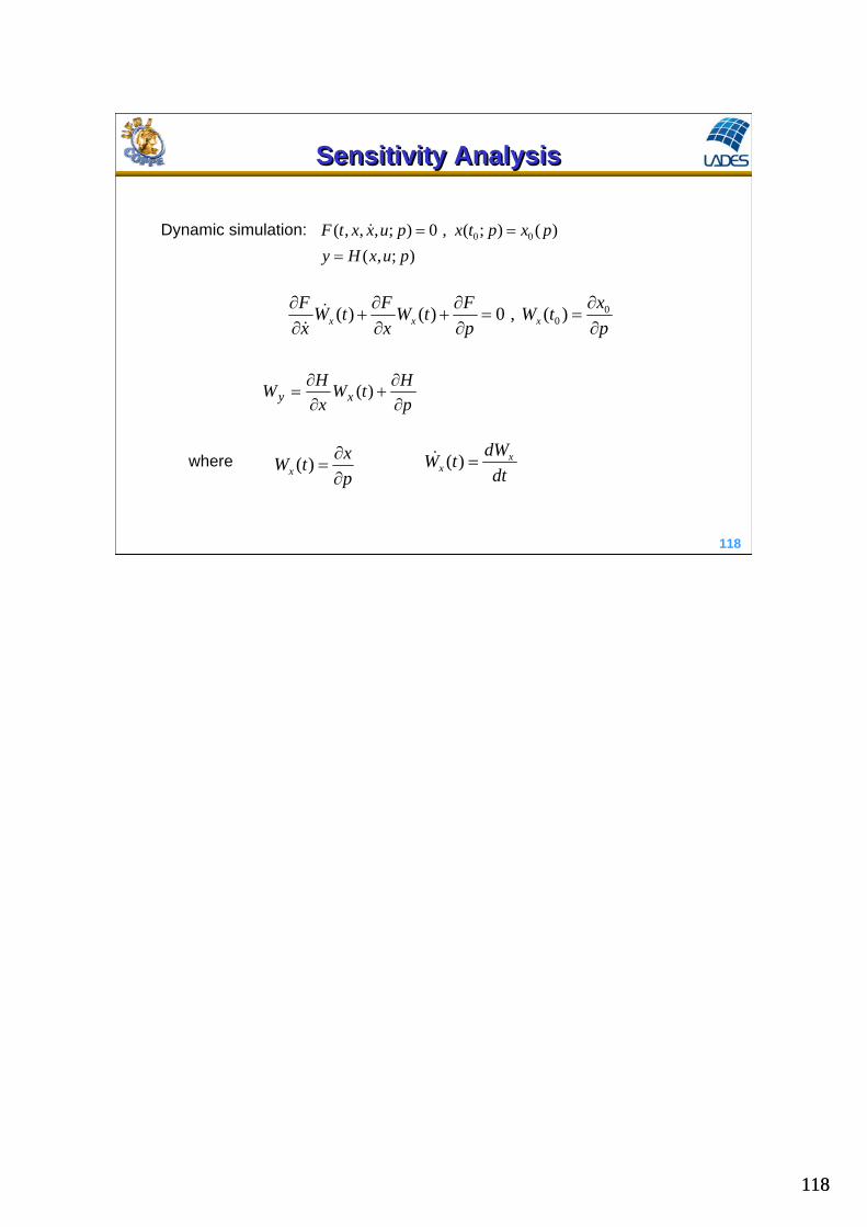
Sensitivity AnalysisSensitivity Analysis
Dynamic simulation: 0 0( , , , ; ) 0 , ( ; ) ( )
( , ; )
F t x x u p x t p x p
y H x u p
00( ) ( ) 0 , ( )x x x
xF F FW t W t W t
x x p p
p
HtW
x
HW xy
)(
where ( ) xx
dWW t
dt( )x
xW t
p

119119
119
Sensitivity AnalysisSensitivity Analysis

120120
120
Sensitivity AnalysisSensitivity Analysis

121
121121
• Integrate a model written in EMSO– Receiving input data from Matlab
– Sending output data to Matlab (discrete mode)
– Sending time derivatives to Matlab (continuous mode)
Interface EMSO-MATLABInterface EMSO-MATLAB
(Similar procedure exists with SCILAB)
122
122122
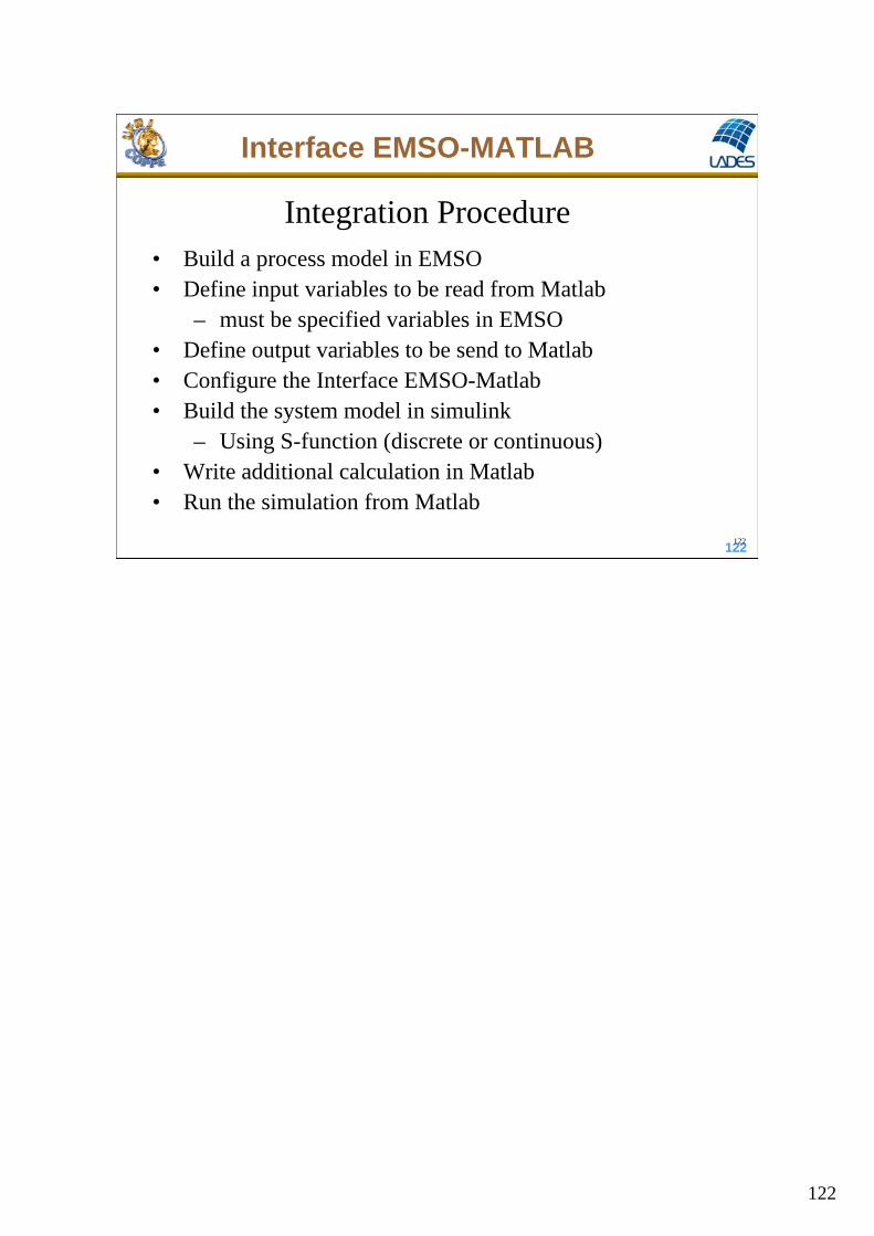
Integration Procedure• Build a process model in EMSO• Define input variables to be read from Matlab
– must be specified variables in EMSO• Define output variables to be send to Matlab• Configure the Interface EMSO-Matlab• Build the system model in simulink
– Using S-function (discrete or continuous)• Write additional calculation in Matlab• Run the simulation from Matlab
Interface EMSO-MATLAB

123
123
• Example: FlashDinamicoSemPID_PFD.mso
Interface EMSO-MATLAB

124
124
• Build the Model – cont.
Interface EMSO-MATLAB

125
125
• Input variables: specifications in EMSO
Interface EMSO-MATLAB

126
126
• Output variables: calculated by EMSO
Interface EMSO-MATLAB

127
127
• Interface configuration – EMSO-Matlab
Interface EMSO-MATLAB

128
128
• Build System in Simulink – without PID
Interface EMSO-MATLAB

129
129
• Configuring size of i/o ports
Interface EMSO-MATLAB

130
130
Interface EMSO-MATLAB
131
131
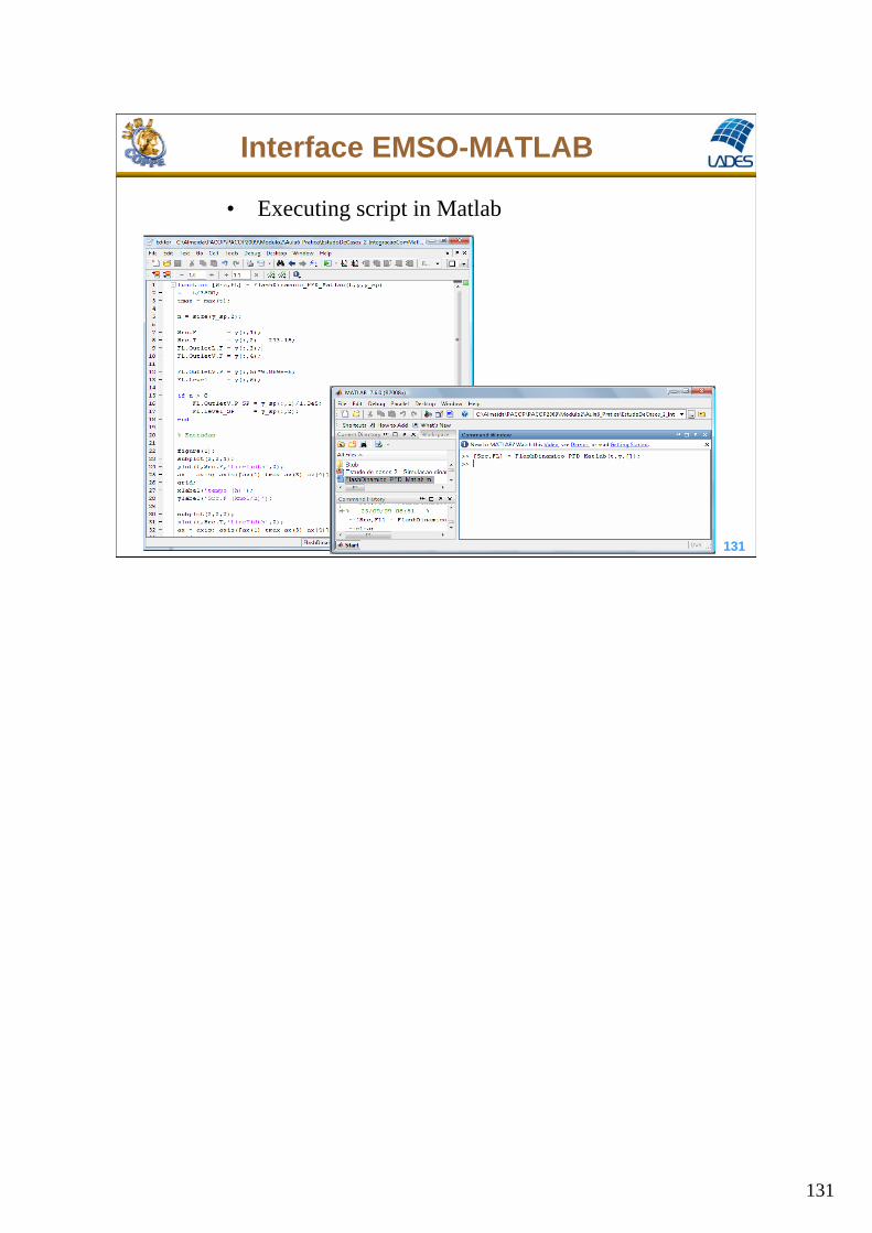
• Executing script in Matlab
Interface EMSO-MATLAB

132
132
• Visualizing Results
Input variables
Output variables
Interface EMSO-MATLAB

133
133
• Build System in Simulink – with PID
Interface EMSO-MATLAB

134
134
• Configuring size of i/o ports
Interface EMSO-MATLAB

135
135
Interface EMSO-MATLAB

136
136
Interface EMSO-MATLAB
• Visualizing Results
Input variables
Output variables

137
137
5. Debugging Techniques5. Debugging Techniques
Questions to be answered to assist the user of a CAPE tool - debugging:
• For an under-constrained model which variables can be fixed or specified?
• For an over-constrained model which equations should be removed?
• For dynamic simulations, which variables can be supplied as initial conditions?
• How to report the inconsistencies making it easy to fix?
In other words, debugging methods need to go beyond degrees of freedom and
the currently available index analysis methods
138
138
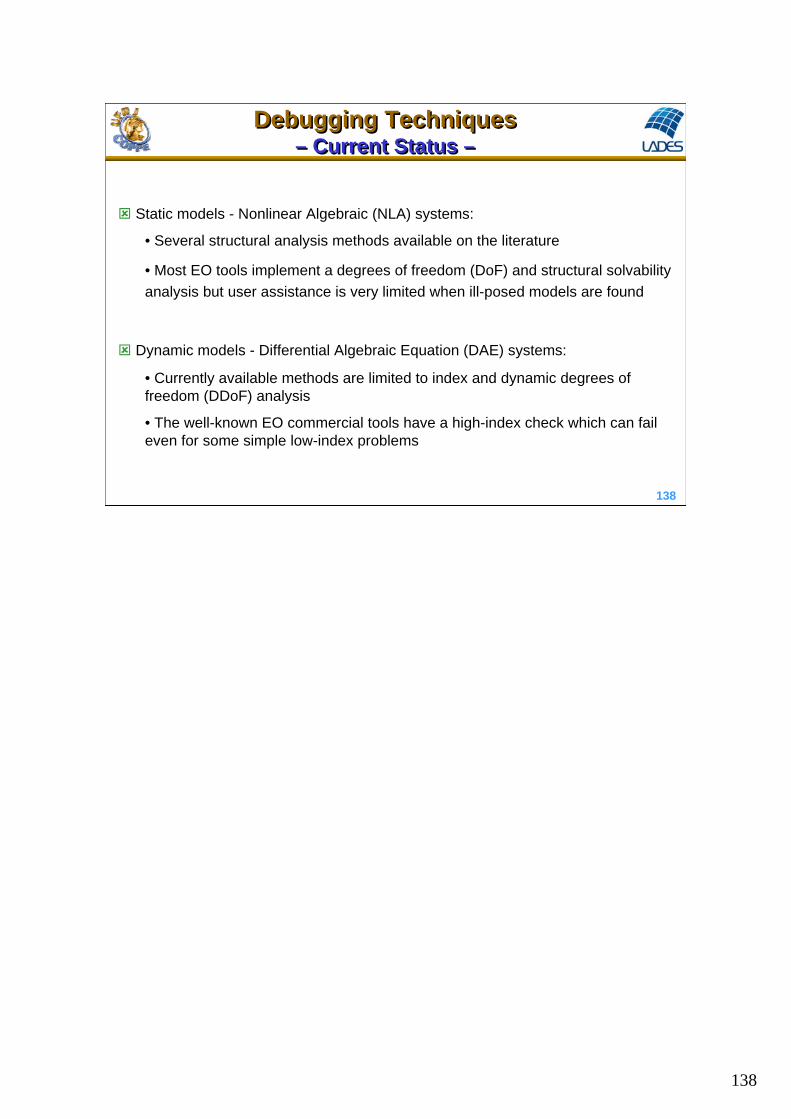
Debugging Techniques– Current Status –
Debugging Techniques– Current Status –
Static models - Nonlinear Algebraic (NLA) systems:
• Several structural analysis methods available on the literature
• Most EO tools implement a degrees of freedom (DoF) and structural solvability
analysis but user assistance is very limited when ill-posed models are found
Dynamic models - Differential Algebraic Equation (DAE) systems:
• Currently available methods are limited to index and dynamic degrees of freedom (DDoF) analysis
• The well-known EO commercial tools have a high-index check which can fail even for some simple low-index problems

139
139
Debugging Techniques– Bipartite Graphs –
Debugging Techniques– Bipartite Graphs –
Bipartite graphs can be used to solve combinatorial problems:
• Tasks to machines
• Classes to rooms
• Equations to variables
• Bipartite graph G(V = Ve Vv , E) have two independent sets of vertices
• Vertices in the same partition must not be adjacent
• We can have alternating and augmenting paths
1 2 3 4
5 6 7 8
Matching {{1,5}, {3,7}} w/ alternating path
Matching {{1,5}, {3,6}, {4,7}} w/ augmenting path

140
140
Debugging Techniques– Bipartite Graphs: variable-equations –
Debugging Techniques– Bipartite Graphs: variable-equations –
Graph for variable-equation relationship
f1(x1) = 0
f2(x1, x2) = 0
f3(x1, x2) = 0
f4(x2, x3, x4) = 0
f5(x4, x5) = 0
f6(x3, x4, x5) = 0
f7(x5, x6, x7) = 0
variables values or equations forms are irrelevant
Maximum MatchingMultiple Solutions

141
141
Debugging Techniques– Nonlinear Algebraic Equations –
Debugging Techniques– Nonlinear Algebraic Equations –
Debugging Nonlinear Problems
Discover if there are over or under-constrained partitions
Start from unconnected vertices and walk in alternating paths
Dulmage and Mendelsohn (DM) decomposition

142
142
Debugging Techniques– Differential-Algebraic Equations –
Debugging Techniques– Differential-Algebraic Equations –
A Simple Example
Solution:
1 2
2
( )
( )
x x a t
x b t
1 1 0
2
( ) (0) ( ) ( )
( ) ( )
tx t x a d b t
x t b t
Only two differential variables
Index-1 system
Requires only one initial condition
Initial condition must be x1
x1 is the only state of the model
143
143
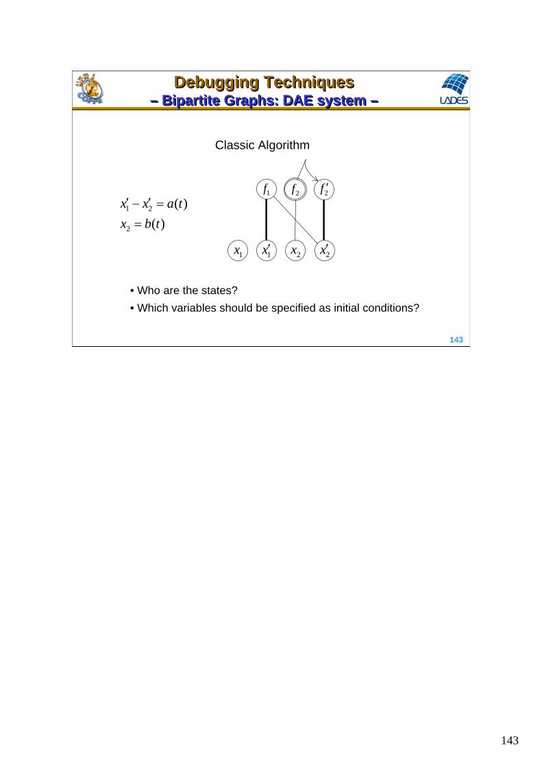
Debugging Techniques– Bipartite Graphs: DAE system –
Debugging Techniques– Bipartite Graphs: DAE system –
1 2
2
( )
( )
x x a t
x b t
1x 2x1x 2x
Classic Algorithm
1f 2f 2f
• Who are the states?
• Which variables should be specified as initial conditions?

144
144
Debugging Techniques– gPROMS output –
Debugging Techniques– gPROMS output –
1 2
2
( )
( )
x x a t
x b t
If only one initial condition is given (which is correct):
145
145
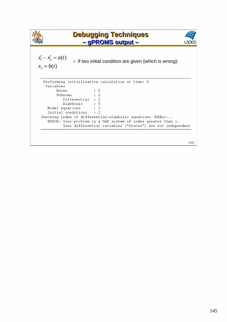
Debugging Techniques– gPROMS output –
Debugging Techniques– gPROMS output –
1 2
2
( )
( )
x x a t
x b t
If two initial condition are given (which is wrong):

146
146
Debugging Techniques– AspenDynamics output –Debugging Techniques– AspenDynamics output –
1 2
2
( )
( )
x x a t
x b t

147
147
Debugging Techniques– New Algorithm: debugging DAE system –
Debugging Techniques– New Algorithm: debugging DAE system –

148
148
Debugging Techniques– New Algorithm: debugging DAE system –
Debugging Techniques– New Algorithm: debugging DAE system –

149
149
Debugging Techniques– Applying the New Algorithm –
Debugging Techniques– Applying the New Algorithm –
1 2
2
( )
( )
x x a t
x b t
1x 2x1x 2x
1f 2f 2f
All equations and all x´ are connected when it finishes
Free variable nodes are the real states
DM decomposition can be applied to the final matching
Singularities are detected (classic algorithm runs indefinitely)
1x 2x
1f 2f 2f
Classic Algorithm

150
150
Debugging Techniques– EMSO output –
Debugging Techniques– EMSO output –
1 2
2
( )
( )
x x a t
x b t
If only one initial condition is given (which is correct):
151
151
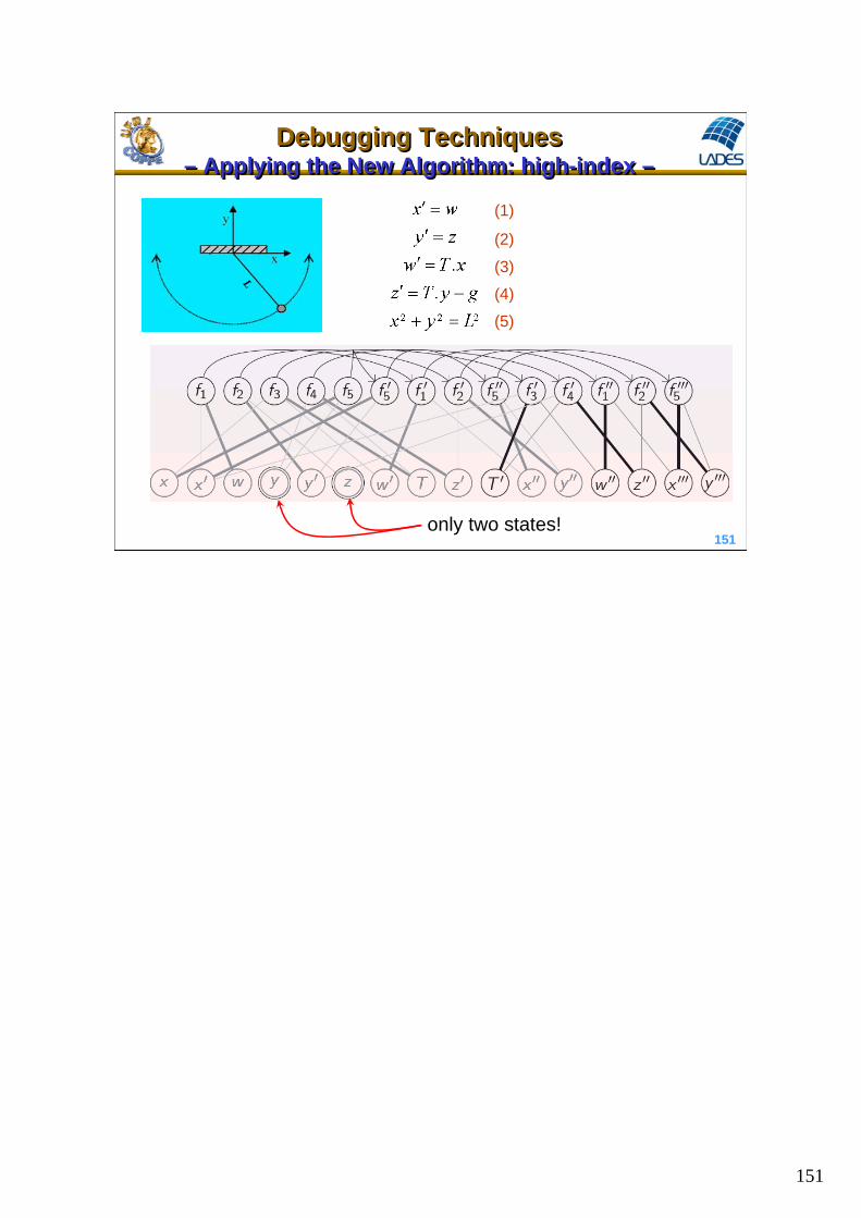
Debugging Techniques– Applying the New Algorithm: high-index –
Debugging Techniques– Applying the New Algorithm: high-index –
L
(1)
(2)
(3)
(4)
(5)
only two states!

152
152
Debugging Techniques– Applying the New Algorithm: performance –
Debugging Techniques– Applying the New Algorithm: performance –
Dynamic model of a distillation column for the
separation of isobutane from a mixture of 13 compounds
* Pentium M 1.7 GHz PC with 2 MB of cache memory, Ubuntu Linux 6.06

153
153
Other CAPE toolsOther CAPE tools
154
154
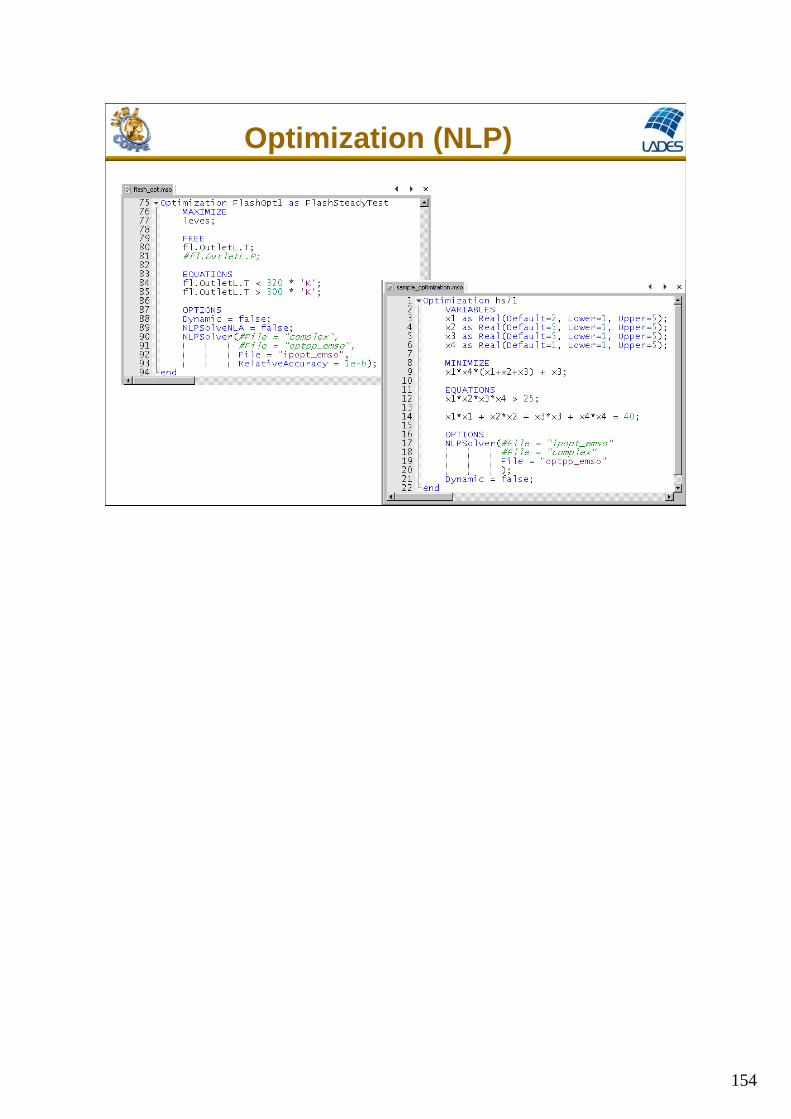
Optimization (NLP)

155
155
Optimization (MINLP)

156
156
Parameter Estimation

157
157
Data Reconciliation

158
158
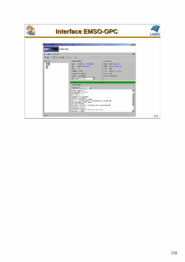
Interface EMSO-OPCInterface EMSO-OPC
Support to the following possible applications:
• Virtual analyzer (inferences with models)
• Process monitoring
• Testing control systems
• Operator training
• State estimators
• Model updating
• Any application that needs integrating models with plant data in real time!
159
159
Interface EMSO-OPCInterface EMSO-OPC

160
160
Interface EMSO-OPCInterface EMSO-OPC
Simulator
Plant

161
161
Operator Training and Process MonitoringOperator Training and Process Monitoring
OPC Server
162
162
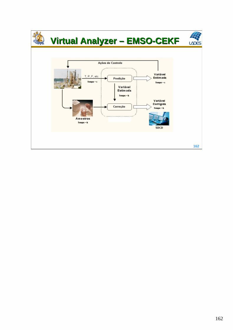
Virtual Analyzer – EMSO-CEKFVirtual Analyzer – EMSO-CEKF

163
163
EMSO-CEKFModel parameters and variables selection

164
164
EMSO-CEKFParameters and variables configuration

165
165
Model Generation for MPCModel Generation for MPC
Process + Regulatory Control
MPC
Data treatment and data reconciliation
Model updating for MPC
Local optimization
Inferences
u(t)y(t)
Y(t)
goals
Model Server(rigorous, empiric, hybrid, reduced)
d(t)

166
166
Model Generation for MPCVariables selection

167
167
Variables configuration
Model Generation for MPC

168
168
Standard InterfacesStandard Interfaces
CAPE-OPEN

169
169
CAPE OPENCAPE OPEN
Example of CAPE-OPEN: DyOS (Dynamic Optimization Software) -Marquardt’s group (2000)
gPROMS

170
170
CAPE OPENCAPE OPEN
Another example of CAPE-OPEN: EMSO (Environment for Modeling, Simulation andOptimization) - Soares and Secchi (2004)
methanol plant
CORBA Object Bus
EMSO BEMSO A
ESO ESO
EMSO ESO

171
171
Momentum
Balance
Overall heat transfer
coefficient evaluation
Energy Balance
Mass Balance
Interface EMSO-CFDInterface EMSO-CFD
Case study using PHOENICS and FLUENT

172
172
Final RemarksFinal Remarks
• The concepts of inheritance and aggregation of the object-oriented modeling paradigm make possible to refine, reuse, and extend available models to more specialized applications, reducing considerably the modeling stage of a project
• A complete consistency analysis of process models described by differential-algebraic equation systems is a very important mechanism to aid the development of new models, specially for large-scale systems
• The integration of a process simulator with model-based tools, such as AUTO and Simulink/Scicos, allows us to carry out more complex analysis of rigorous models and complete flowsheetsimulations

173
173
Final RemarksFinal Remarks
• Process simulators and optimizers
• System identification packages
• System analysis
• Standard communication interfaces
• Numerical solvers (NLA, NLP, MINLP, DAE, ...)
• User-friendly graphical interfaces
Available CAPE tools ...
... that need high-tech people to use and improve them!

174
174
ReferencesReferences
• Andersson, M. 1994. Object-oriented modeling and simulation of hybrid systems. Ph.D. diss., Department of Automatic Control, Lund Institute of Technology, Lund, Sweden.
• Barton, P.I. 1999. ABACUSS II. Retrieved from http://yoric.mit.edu/abacuss2/abacuss2.html
• Barton, P.I. and Pantelides, C.C., 1994, The modeling of combined discrete=continuous processes, AIChE J., 40, 966–979.
• Bogusch, R., Lohmann, B., Marquardt, W. 2001. Computer-aided process modeling with MODKIT. Comp. & Chem. Engng., 25, 963–995.
• Bogusch, R. and Marquardt, W. 1997. A formal representation of process model equations. Comp. & Chem. Engng. 21 (10) 1105-111.
• EA International and ESA. 1999. EcosimPro ver. 3.0: Getting started, users manual, modeling language (EL), modeling and simulation guide, and mathematical algorithms. Madrid, Spain: EA International.
• Eliceche, A.M., Corvalán, S.M. and Martinez, P.E. 2007. Environmental Life Cycle Impact as a Tool for Process Optimization of a Utility Plant. Comp. & Chem. Engng., 31, 648–656.
• Elmqvist, H. 1978. A structured model language for large continuous systems. Ph.D. diss., Lund Institute of Technology, Lund, Sweden.
• Elmqvist, H., D. Bruck, and M. Otter. 1999. Dymola: Dynamic modeling laboratory: User’s manual.Version 4.0. Lund, Sweden: Dynamic AB.
• Halim, I. and Srinivasan, R. 2011. A Knowledge-Based Simulation-Optimization Framework and System for Sustainable Process Operations. Comp. & Chem. Engng., 35, 92–105.
• Heijungs, R., Guinée, J., Huppes, G., Lankreijer, R.M., Ansems, A.A.M., Eggels, P.G., van Duin, R and. de Goede, H.P. 1992. Environmental Life Cycle Assessment of Products-Guide and Backgrounds. Centre of Environmental Science (CML). Leiden.

175
175
ReferencesReferences• Jia, X.P., Han, F.Y. and Tan, X.S. 2004. Integrated Environmental Performance Assessment of Chemical Processes. Comp. & Chem. Engng., 29, 243–247.
•Modelica Association. 1996. Modelica: A unified object-oriented language for physical systems modeling: Tutorial, rationale and language specification. Retrieved from http://www.modelica.org.
• Piela, P.C. 1989. ASCEND:Anobject-oriented environment for modeling and analysis. Ph.D. diss., Engineering Design Research Center, Carnegie Mellon University, Pittsburgh, PA.
• Rao, R.M., Rengaswamy, R., Suresh, A.K. and Balaraman, K.S. 2004. Industrial Experience with Object-Oriented Modelling FCC Case Study. Chem. Engng. Res. & Des., 82 (A4) 527–552.
• Rodrigues, R., Soares, R.P. and Secchi, A.R. 2010. Teaching Chemical Reaction Engineering Using EMSO Simulator. Computer Applications in Engineering Education, 18 (4) 607-618.
• Salau, N.P.G., Neumann, G.A, Trierweiler, J.O. and Secchi, A.R. 2008. Dynamic Behavior and Control in an Industrial Fluidized-Bed Polymerization Reactor. Ind. Eng. Chem. Res., 47, 6058–6069.
• Soares, R.P. and Secchi, A.R. 2003. EMSO: A New Environment for Modeling, Simulation and Optimization. ESCAPE 13, Lappeenranta, Finlândia, 947 – 952.
• Soares, R.P. and Secchi, A.R. 2005. Direct Initialisation and Solution of High-Index DAE Systems, ESCAPE 15, Barcelona, Spain, 157–162.
• Soares, R.P. and Secchi, A.R. 2007. Debugging Static and Dynamic Rigorous Models for Equation-oriented CAPE Tools, DYCOPS 2007, Cancún, Mexico, 2, 291–296.
•Tränkle, E, Gerstlauer, A., Zeitz, M., and Gilles, E. D. 1997.The Object-Oriented Model Definition Language MDL of the Knowledge-Based Process Modeling Tool PROMOT. In A. Sydow (Ed.), 15th IMACS World Congress, Berlin, Germany, 4, 91-96.
• Valle, E.C., Soares, R.P., Finkler, T.F. and Secchi, A.R. 2008. A New Tool Providing an Integrated Framework for Process Optimization, EngOpt 2008 - International Conference on Engineering Optimization, Rio de Janeiro, Brazil.

176
176
ReferencesReferences
DAE Solvers:
DASSL: Petzold, L.R. (1989), http://www.enq.ufrgs.br/enqlib/numeric/numeric.html
DASSLC: Secchi, A.R. (1992), http://www.enq.ufrgs.br/enqlib/numeric/numeric.html
MEBDFI: Abdulla, T.J. and J.R. Cash (1999), http://www.netlib.org/ode/mebdfi.f
PSIDE: Lioen, W.M., J.J.B. de Swart, and W.A. van der Veen (1997), http://www.cwi.nl/cwi/projects/PSIDE/
SUNDIALS: Serban, R. et al. (2004), http://www.llnl.gov/CASC/sundials/description/description.html

177
177
... thank you for your attention!
Process Modeling, Simulation and Control LabProcess Modeling, Simulation and Control Lab
•• Prof. Dr. Argimiro Prof. Dr. Argimiro ResendeResende SecchiSecchi
•• Phone: +55Phone: +55--2121--25622562--83018301
•• EE--mail: mail: [email protected]@peq.coppe.ufrj.br•• http://http://www.peq.coppe.ufrj.br/Areas/Modelagem_e_simulacao.htmlwww.peq.coppe.ufrj.br/Areas/Modelagem_e_simulacao.html
http://www.enq.ufrgs.br/alsoc
PASI 2011Process Modeling and Optimization for Energy and Sustainability
Solutions for Process Control and OptimizationSolutions for Process Control and Optimization

178
178
Extra slidesExtra slides

179
179
EMSO Tutorial– Modeling Structure –
EMSO Tutorial– Modeling Structure –
EMSO has 3 main entities in the modeling structure
FlowSheetFlowSheet – process model, is composed by a set of DEVICESDEVICES
DEVICESDEVICES – components of a FlowSheet, an unit operation or an equipment
ModelModel – mathematical description of a DEVICE

180
180
ModelModel FlowSheetFlowSheet
ModelModel: equation: equation--basedbased FlowSheetFlowSheet: component: component--basedbased
EMSO Tutorial– Modeling Structure –
EMSO Tutorial– Modeling Structure –
streamPH
181
181
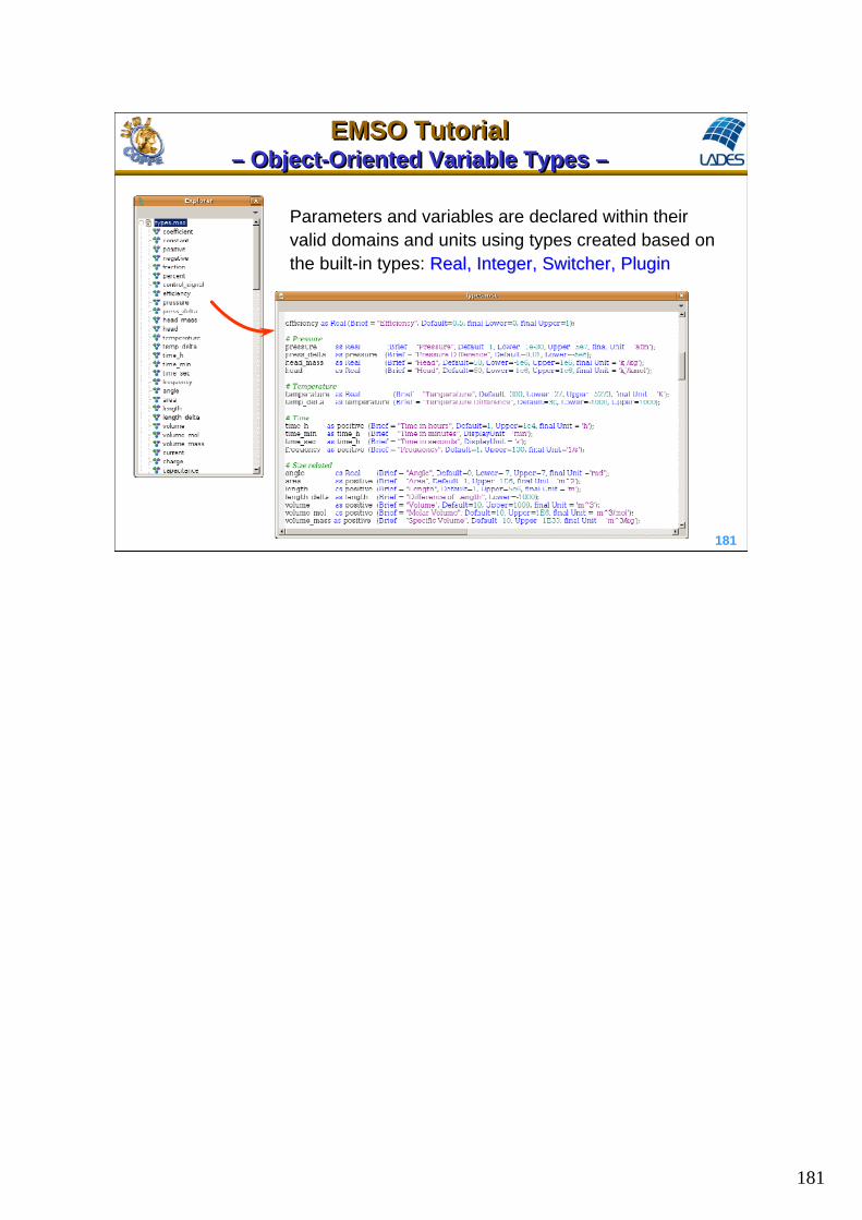
Parameters and variables are declared within their valid domains and units using types created based on the built-in types: Real, Integer, Switcher, Real, Integer, Switcher, PluginPlugin
EMSO Tutorial– Object-Oriented Variable Types –
EMSO Tutorial– Object-Oriented Variable Types –

182
182
EMSO Tutorial– Model Components –
EMSO Tutorial– Model Components –
Including sub-models and types
Automatic model documentation
Symbol of variable in LaTeX command for
documentation
Basic sections to create a
math. modelPort location to draw a flowsheet connection
Input and output connections

183
183
EMSO Tutorial– FlowSheet Components –
EMSO Tutorial– FlowSheet Components –
Degree of Freedom
Dynamic Degree of Freedom
Simulation options
Parameters of DEVICES

184
184
EMSO Tutorial– Checking Units of Measurement –
EMSO Tutorial– Checking Units of Measurement –
incompatible units

185
185
Flash multi-component
m
V, y
L, x
F, z, Pf, Tf
T, P
EMSO Tutorial– A simple example –
EMSO Tutorial– A simple example –

186
186
A liquid-phase mixture of C hydrocarbons, at given temperature and
pressure, is heated and continuously fed into a vessel drum at lower
pressure, occurring partial vaporization. The liquid and vapor phases are
continuously removed from the vessel through level and pressure
control valves, respectively. Determine the time evolution of liquid and
vapor stream composition and the vessel temperature and pressure,
due to variations in the feed stream, keeping the heating rate constant.
EMSO Tutorial– FLASH: process description –
EMSO Tutorial– FLASH: process description –

187
187
• negligible vapor holdup (no dynamics in vapor phase);
• thermodynamic equilibrium (ideal stage);
• no droplet drag in vapor stream;
• negligible heat loss to surroundings;
• (internal energy) (liquid-phase enthalpy);
• perfect mixture in both phases.
EMSO Tutorial– FLASH: model assumptions –
EMSO Tutorial– FLASH: model assumptions –

188
188
dmF V L
dt
i i i i
dm x F z V y L x
dt
iii xKy
Overall mass balance (molar base):
(1)
(2) i = 1, 2, ..., C
Component mass balance:
Equilibrium:
Ki = f(T, P, x, y)
(3) i = 1, 2, ..., C
(4) i = 1, 2, ..., C
Molar fraction:
C
iix
1
1 (5)
EMSO Tutorial– FLASH: modeling –
EMSO Tutorial– FLASH: modeling –

189
189
Energy balance:
(6)( ) f
dm h F h q V H L h
dt
Enthalpies:
h = f(T, P, x)
H = f(T, P, y)
hf = f(Tf, Pf, z)
(7)
(8)
(9)
Controllers:
L = f(m)
V = f(P)
(10)
(11)
EMSO Tutorial– FLASH: modeling –
EMSO Tutorial– FLASH: modeling –

190
190
variable units of measurement
m kmol
F, L, V kmol s-1
t s
xi, yi, zi kmol kmol-1
Ki –
T, Tf K
P, Pf kPa
q kJ s-1
h, H, hf kJ kmol-1
EMSO Tutorial– FLASH: consistency analysis –
EMSO Tutorial– FLASH: consistency analysis –

191
191
variables: m, F, L, V, t, xi, yi, zi, Ki, T, Tf, P, Pf, q, h, H, hf 13+4Cconstants: 0specifications: q, t 2driving forces: F, zi, Tf, Pf 3+Cunknown variables: m, L, V, xi, yi, Ki, T, P, h, H, hf 8+3Cequations: 8+3C
Degree of Freedom = variables – constants – specifications – driving forces –equations = unknown variables – equations = (13+4C) – 0 – 2 – (3+C) – (8+3C) = 0
Initial condition: m(0), xi(0), T(0) 2+C
Dynamic Degree of Freedom (index < 2) = differential equations – initial conditions = (2+C) – (2+C) = 0
EMSO Tutorial– FLASH: consistency analysis –
EMSO Tutorial– FLASH: consistency analysis –

192
192
EMSO Tutorial– FLASH: EMSO version –
EMSO Tutorial– FLASH: EMSO version –
Running EMSO
Note: file Sample_flash_pid.mso has level and pressure controllers.

193
193

194
194

195
195
Horizontal axis is always the independent variable (usually time)
EMSO Tutorial– Simulation Results: graphics –
EMSO Tutorial– Simulation Results: graphics –
double-click

196
196
Choose the file format
Right-click the mouse button and select ““Export ImageExport Image””
EMSO Tutorial– Simulation Results: exporting graphics –
EMSO Tutorial– Simulation Results: exporting graphics –

197
197
EMSO Tutorial– Simulation Results: exporting data –
EMSO Tutorial– Simulation Results: exporting data –
Choose the file formatRLT: MATLAB/SCILAB
XML: EXCEL/OpenOffice
click

198
198
Using EXCEL to analyze the results
Results separated by devices
EMSO Tutorial– Simulation Results: in spreadsheets –
EMSO Tutorial– Simulation Results: in spreadsheets –

199
199
EMSO Tutorial– Simulation Results: in MATLAB/SCILAB –
EMSO Tutorial– Simulation Results: in MATLAB/SCILAB –
Using MATLAB to analyze the results

200
200
EMSO Tutorial– Building Block Diagrams: create file –
EMSO Tutorial– Building Block Diagrams: create file –
Selected components
from physical properties package
Devices found in the model
library

201
201
EMSO Tutorial– Building Block Diagrams: select devices –
EMSO Tutorial– Building Block Diagrams: select devices –
click to create a device
drag & drop ports to create a connection
When making a connection, only
compatible ports become
available to connect

202
202
EMSO Tutorial– Building Block Diagrams: set case study –
EMSO Tutorial– Building Block Diagrams: set case study –
double-click
Variable status: unknown (Evaluate)known (Specify)initial condition (Initial)estimate (Guess)

203
203
EMSO Tutorial– Building Block Diagrams: thermodynamic –
EMSO Tutorial– Building Block Diagrams: thermodynamic –
right-click Available models
PC-SAFT
204
204
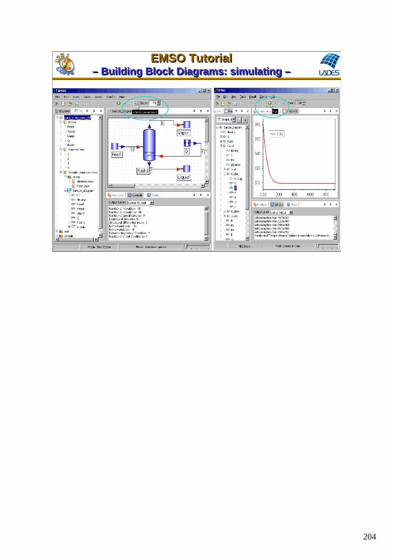
EMSO Tutorial– Building Block Diagrams: simulating –
EMSO Tutorial– Building Block Diagrams: simulating –

205
205
EMSO Tutorial– Automatic Documentation –
EMSO Tutorial– Automatic Documentation –
Note: LaTeX must be installed.

206
206
Some Industrial ApplicationsSome Industrial Applications
Dynamic Simulation of a Propane Refrigeration Cycle of a Natural Gas Processing Unit
207
207
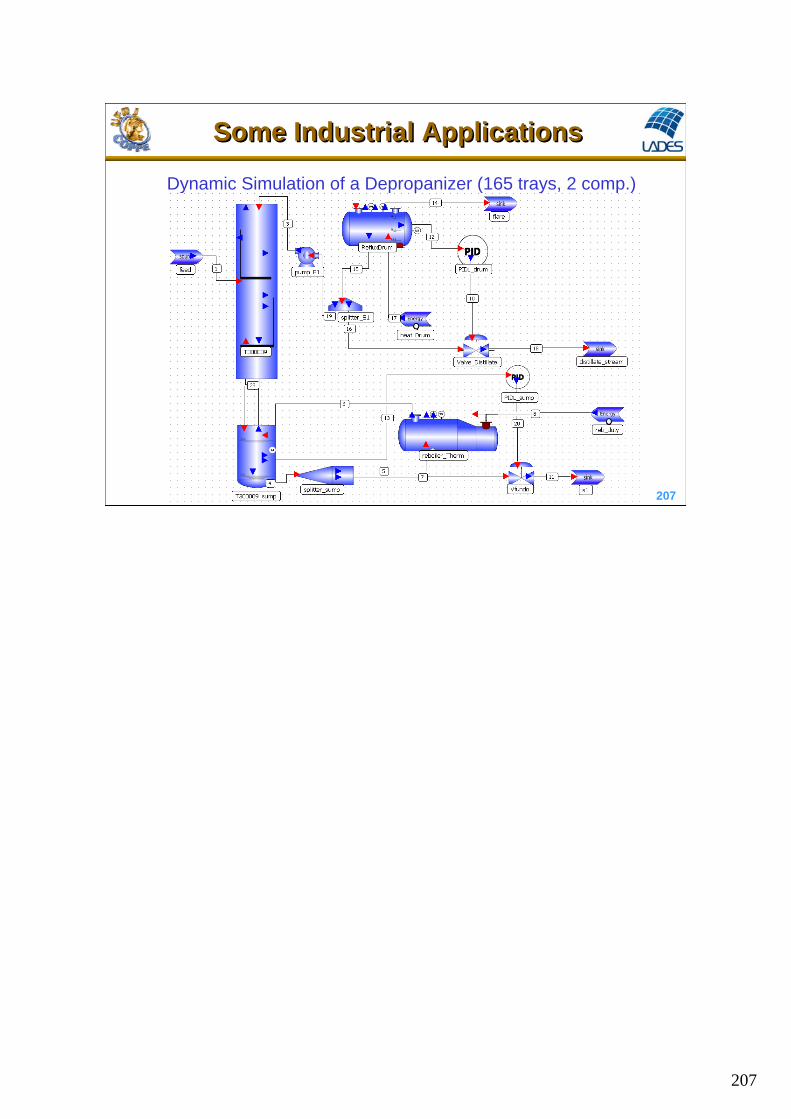
Dynamic Simulation of a Depropanizer (165 trays, 2 comp.)
Some Industrial ApplicationsSome Industrial Applications

208
208
Dynamic Simulation of a Deisobutanizer(80 trays, 13 comp.)
Some Industrial ApplicationsSome Industrial Applications

209
209
Steady-State Simulation of a Power Plant with Pulverized Coal
Some Industrial ApplicationsSome Industrial Applications

210
210
Compounds: OD, TOC, Phenol, NH3, NO2, NO3 and 6 groups of bacteria
Dynamic Simulation of a Industrial Waste Water Treatment Unit (Müller et al., 2009)
Some Industrial ApplicationsSome Industrial Applications

211
211
Dynamic Simulation of a General Purpose Polystyrene Process
Some Industrial ApplicationsSome Industrial Applications

212
212
Method of Orthogonal Collocation with EMSO
EMSOSimulator
RootsA and B Matrices
• Boundaries• Internal Points• Alfa and Beta
• Jacobi roots• A and B matrices
Plugin
DD as Plugin (Type=“OCFEM”, Boundary="BOTH”, InternalPoints=5 alfa=1, beta=1)
Plugin: ocfem_emso.dll

213
213
Fixed-bed Reactor with Axial Dispersion(reaction of order m)
2
2
1 my y yDa y
x Pe x
Boundary conditions:
0
11 ( ,0)
x
yy
Pe x
1
0x
y
x
( ,0) 1y or
Initial conditions:
(0, ) 0y x

214214
214
Example: add Plugin ocfem_emso.dll and execute flowsheets of files FDM_ss.mso, OCM_ss.mso and OCFEM_ss.mso, and compare results of discretizations. Repeat for the dynamic simulation in files FDM_din.mso e OCM_din.mso.
PDEMethod of Lines: D.F. and Orthogonal Collocation
PDEMethod of Lines: D.F. and Orthogonal Collocation

215
215
Comparing Results
OCM by EMSONumber of internal points: 5
y(x=1) = 0.151475 (error of 0.038%)
1 1 Method of Finite DifferencesNumber of internal points: 6000
y(x=1) = 0.15155 (error of 0.087%)
y(x=1) = 0.151418 (exact)

216
216
Case Study
• Production of acetic anhydride in adiabatic PFR– Acetic anhydride is often produced by reacting acetic acid with ketene,
obtained by heating acetone at 700-770oC.
– A important step is the vapor phase cracking of acetone to ketene and methane:
– The second step is the reaction of ketene with acetic acid.
Ref: G. V. Jeffreys, A Problem in Chemical Engineering Design: The Manufacture of Acetic Anhydride, 2nd ed. (London: Institution of Chemical Engineers, 1964)
3 3 2 4C H C O C H C H C O C H
2 3 3CH CO CH COOH CH CO O

217
217
34222exp 34.34k
T
Problem Definition – The first production step is carried out in a vapor phase reaction
of acetone in an adiabatic PFR.
where A = acetone; B = ketene and C = methane
– The reaction is of 1a order in relation to acetone in the cracking reaction, with Arrhenius constant given by:
• k – seconds-1
• T – Kelvin
CBA
Case Study

218
218
Process Description
– Reactor geometry• adiabatic continuous tubular reactor;• bank of 1000 tubes of 1 in sch. 40 with cross section of 0.557 m2;• total length of 2.28 m;
– Operating conditions• feed temperature 762oC (1035 K);• operating pressure: 1.6 atm• feed flow rate of 8000 kg/h (137.9 kmol/h);
– Composition• acetone, ketene and methane• feed of pure acetone
– Kinetics• first order reaction, • pre-exponential factor (k0): 8.2 x 10¹⁴ s-1
• activation energy (E/R): 34222 K• heat of reaction: -80.77 kJ/mol
Case Study
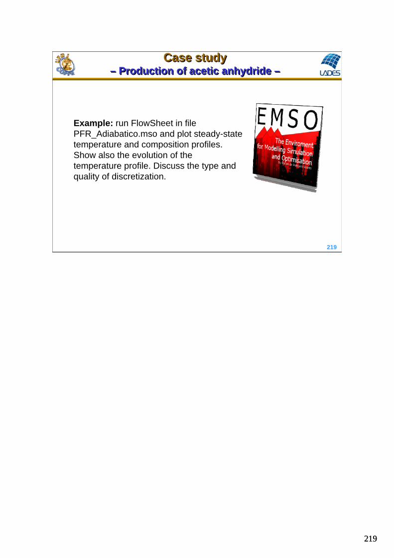
219219
219
Example: run FlowSheet in file PFR_Adiabatico.mso and plot steady-state temperature and composition profiles. Show also the evolution of the temperature profile. Discuss the type and quality of discretization.
Case study– Production of acetic anhydride –
Case study– Production of acetic anhydride –