proceedings of the 2016 winter simulation conference t. m

Proceedings of the 2016 Winter Simulation Conference T. M. K. Roeder, P. I. Frazier, R. Szechtman, E. Zhou, T. Huschka, and S. E. Chick, eds.

KNOWLEDGE DISCOVERY IN SIMULATION DATA: A CASE STUDY OF A GOLD MINING FACILITY

Niclas Feldkamp Sören Bergmann

Steffen Strassburger

Thomas Schulze

Department for Industrial Information Systems School of Computer Science

Ilmenau University of Technology Otto-von-Guericke-University Magdeburg P.O. Box 100 565 Universitätsplatz 2

98684 Ilmenau, GERMANY 39106 Magdeburg, GERMANY

ABSTRACT

Discrete event simulation is an established methodology for investigating the dynamic behavior of complex systems. Apart from conventional simulation studies, which focus on single model aspects and answering specific analysis questions, new methods of broad scale experiment design and analysis emerge in alignment with new possibilities of computation and data processing. This paper outlines a visually aided process for knowledge discovery in simulation data which is applied onto a real world case study of a mining facility in Western Australia.

1 INTRODUCTION

Discrete event simulation is a broadly accepted methodology for planning new production and logistic systems, or for evaluating and improving existing ones. Traditionally, simulation studies focus on a specifically outlined project scope, guided by concrete and quantifiable questions in a way that conducting experiments is performed by varying distinct and preselected parameters that are supposed to be influential to the simulation project goal (Law 2014). Apart from conventional simulation studies, new forms and methods of simulation based applications have recently been developed.

Those leverage new possibilities through recent advancements in computing power and database technology. These recent advancements in computing power enable to conduct large and broad scale simulation ensembles (Matkovic et al. 2015; Theodoropoulos 2015). In previous papers, we outlined an approach called knowledge discovery in manufacturing simulations that is based on large scale simulation experiments and introduced new possibilities of simulation data analysis led by data mining and visual representations (Feldkamp et al. 2015a). This approach primarily supports the idea of finding interesting patterns and relations in the simulation data that have been unknown beforehand. While in previous work this was demonstrated and validated by simple academic models, here we apply our approach on a real world simulation model of an underground gold mine.

The remainder of this paper is structured as follows: In section 2 we introduce related work on data farming, visual analytics and knowledge discovery in simulation data. In section 3 the mine and the underlying circumstances of the simulation model are described, as well as the general setup, experimental design and analysis procedure. Section 4 discusses selected results of the case study investigation followed by a conclusion and future work discussion in section 5.

978-1-5090-4486-3/16/$31.00 ©2016 IEEE 1607

Feldkamp, Bergmann, Strassburger, and Schulze

2 RELATED WORK: KNOWLEDGE DISCOVERY IN SIMULATION DATA

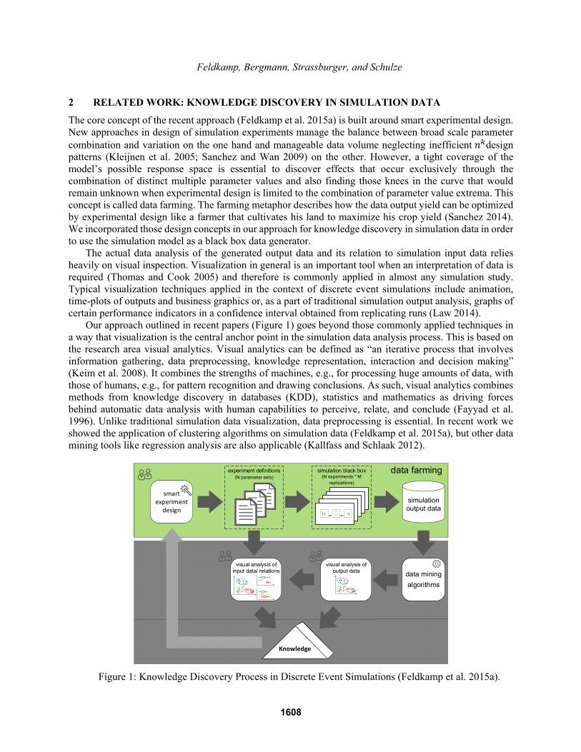
The core concept of the recent approach (Feldkamp et al. 2015a) is built around smart experimental design. New approaches in design of simulation experiments manage the balance between broad scale parameter combination and variation on the one hand and manageable data volume neglecting inefficient design patterns (Kleijnen et al. 2005; Sanchez and Wan 2009) on the other. However, a tight coverage of the model’s possible response space is essential to discover effects that occur exclusively through the combination of distinct multiple parameter values and also finding those knees in the curve that would remain unknown when experimental design is limited to the combination of parameter value extrema. This concept is called data farming. The farming metaphor describes how the data output yield can be optimized by experimental design like a farmer that cultivates his land to maximize his crop yield (Sanchez 2014). We incorporated those design concepts in our approach for knowledge discovery in simulation data in order to use the simulation model as a black box data generator.

The actual data analysis of the generated output data and its relation to simulation input data relies heavily on visual inspection. Visualization in general is an important tool when an interpretation of data is required (Thomas and Cook 2005) and therefore is commonly applied in almost any simulation study. Typical visualization techniques applied in the context of discrete event simulations include animation, time-plots of outputs and business graphics or, as a part of traditional simulation output analysis, graphs of certain performance indicators in a confidence interval obtained from replicating runs (Law 2014).

Our approach outlined in recent papers (Figure 1) goes beyond those commonly applied techniques in a way that visualization is the central anchor point in the simulation data analysis process. This is based on the research area visual analytics. Visual analytics can be defined as “an iterative process that involves information gathering, data preprocessing, knowledge representation, interaction and decision making” (Keim et al. 2008). It combines the strengths of machines, e.g., for processing huge amounts of data, with those of humans, e.g., for pattern recognition and drawing conclusions. As such, visual analytics combines methods from knowledge discovery in databases (KDD), statistics and mathematics as driving forces behind automatic data analysis with human capabilities to perceive, relate, and conclude (Fayyad et al. 1996). Unlike traditional simulation data visualization, data preprocessing is essential. In recent work we showed the application of clustering algorithms on simulation data (Feldkamp et al. 2015a), but other data mining tools like regression analysis are also applicable (Kallfass and Schlaak 2012).

data farming

smart experiment

design

experiment definitions (N parameter sets)

simulation output data

simulation black box(N experiments * M

replications)

data mining

algorithms

Knowledge

visual analysis of output data

visual analysis of input data/ relations

+ +++

++++

+++ + +

++

+++

++

+

++ ++ +++

++++

+++ + +

++

+++

++

+

++ +

Figure 1: Knowledge Discovery Process in Discrete Event Simulations (Feldkamp et al. 2015a).

1608

Feldkamp, Bergmann, Strassburger, and Schulze In order to investigate simulation data preprocessed by data mining algorithms, we investigated suitable

visualization and interaction methods in a recent work (Feldkamp et al. 2015b; Feldkamp et al. 2016). The portfolio of diagram types mainly fall in two categories: One is for coarse assessment of data and estimation of parameter value distribution to begin with, the other is for the in depth analysis of data subsets that usually follows throughout this process. Furthermore, visualization types in the second category benefit the most from options of interaction, mainly selection, filtering and coloring of data. Also, rotating camera angles as well as zooming in and out may be beneficial in 3D plots.

3 CASE STUDY

3.1 Background

Investigations in this case study are carried out on a simulation and animation model of an underground gold mine.

As today, the mine currently operates only on a campaign basis on a level of 1100 meters below surface. With increasing gold prices as external condition, evaluations of possibilities for re-opening the facility permanently and even descending to lower loading levels have been investigated with the existing simulation model.

Figure 2: Top: 2D-Layout of the decline. Bottom left side: 3D-Model of the decline. Bottom right side: 3D-Model of a mining haul truck traveling down the decline.

Figure 2 shows layout and 3D screenshots of the model. The constructed simulation model represents the current state of operating the mine with loading ports at 1100 and 1200 meters below the surface. Loading ports are those areas where mined material is loaded onto trucks, which then hauls the material up to a port at 125 meters below sea level where the facility switches from underground to opencast mining. At this port, haul trucks dump their load which then can be processed and separated into valuable ore and waste. This dumping port furthermore marks the boundary of the simulation model, so that the main focus here is the transportation of material from the loading port to the dumping port. Daily limit for the quantity

1609


of conveyed material is about 5000 tons per day, as this is the daily limit for the following material processing at the surface.

Additional loading ports deeper than 1200 meters below surface are already implemented in the model, so an investigation of scenarios with deeper loading points is possible. Furthermore, the model takes into account the impact and interaction of equipment breakdown so that haul trucks have to visit a workshop located at the surface for scheduled and unplanned maintenance. A truck driver decides after dumping whether or not he has to drive to a workshop. The transportation routes are modeled on very detailed, microscopic scale. On its route, a haul truck has to interact with other trucks and/or light vehicles. Finally, a shift regime is implemented that influences active work hours as well as pausing times within and between shifts. With the application of the knowledge discovery concept, mining engineers can get some new or additional insights into the model. Besides conveying unknown and interesting patterns, the visual investigation is guided by some coarse analysis questions that are described below.

3.2 Description of Questions

The main application of the knowledge discovery in simulation data concept is conveying interesting patterns and relations between all modeled input and output parameters. Additionally, in this case study the configuration of trucks is of peculiar interest. Configuration refers to number and tonnage of the haul trucks. Because leasing contracts are rather long term and inflexible, a constellation of trucks that performs well at the base level (1100 meters) and remains well if the company decides to go deeper is a very interesting question. From that we derive three coarse investigation questions to guide the discussion of results:

1. Are there any interesting patterns and relations in the simulation data that may create additional

knowledge for the mining engineers? 2. Which configuration of haul trucks performs consistently well at base level 1100? 3. How does it hold up against deeper loading levels and how do performance and cost parameters

alter when depth of loading points increases?

3.3 Experimental Design

Adjustable input factors have been split up into two categories, which are decision and noise factors. Decision factors are those parameters that are influenceable by the decision-maker, whereas noise factors are not. Table 1 shows a list of input factors with their corresponding parameter value range and type level of measurement.

Table 1: Input Factors for the simulation experiments.

Factor Margin Scale Description Decision Factors

#Trucks 1 – 20 discrete number of haul trucks Tonnage [20-50]

(increments of 10) categorical payload of a haul truck in ton

LoadingPort [1100-2000] (increments of 100)

categorical depth of loading port in meters below surface

Shift 9 - 11 discrete shift regime with active shift duration in hours Noise Factors

SpeedDown 8 - 14 continuous truck down driving speed in km/h LoadingTime 2 - 5 continuous loading time for a haul truck in minutes WorkshopRate 10 - 20 continuous probability for unscheduled maintenance

1610

Feldkamp, Bergmann, Strassburger, and Schulze Note that in addition to the noise factors margin, we also incorporated a small stochastic deviation for

each noise factor in a way that we replicated every design point ten times. Furthermore, the depth of the loading port stands out from other decision factors in a way that the influence of the loading port depth is obviously tremendous and creates different scenarios rather than a variation of a simple input parameter. In fact, investigating each loading port scenario as well as the investigation of parameter distribution over different depth levels might give some interesting insights in the model.

With the given number of factors and margins, a full factorial design would not be feasible (Sanchez 2007). Therefore, we used a design of experiment method called nearly balanced nearly orthogonal hypercube design (Vieira et al. 2011). We created one design for each of the two input factor categories. Finally, those designs were crossed to investigate the distribution and robustness of the decision factors against the noise factors. This resulted in an experiment table with 262,144 design points. Each simulation run simulates a period of 31 days, with a warm up period of one day and 30 days for result data collection after the warm up.

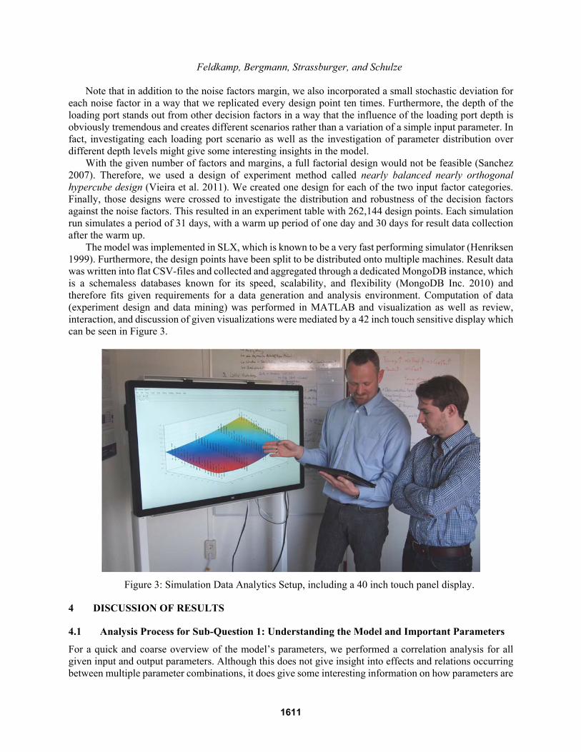
The model was implemented in SLX, which is known to be a very fast performing simulator (Henriksen 1999). Furthermore, the design points have been split to be distributed onto multiple machines. Result data was written into flat CSV-files and collected and aggregated through a dedicated MongoDB instance, which is a schemaless databases known for its speed, scalability, and flexibility (MongoDB Inc. 2010) and therefore fits given requirements for a data generation and analysis environment. Computation of data (experiment design and data mining) was performed in MATLAB and visualization as well as review, interaction, and discussion of given visualizations were mediated by a 42 inch touch sensitive display which can be seen in Figure 3.

Figure 3: Simulation Data Analytics Setup, including a 40 inch touch panel display.

4 DISCUSSION OF RESULTS

4.1 Analysis Process for Sub-Question 1: Understanding the Model and Important Parameters

For a quick and coarse overview of the model’s parameters, we performed a correlation analysis for all given input and output parameters. Although this does not give insight into effects and relations occurring between multiple parameter combinations, it does give some interesting information on how parameters are

1611


linked to each other pairwise. Table 2 shows the corresponding correlation matrix. Note that parameter one to seven are input parameters, whereas the following ones are output parameters. Therefore, the correlation between input parameters seen in the first quadrant is not relevant. In fact, in order to create a good experiment design, input parameters should have a minimum correlation. Furthermore, the bottom right quadrant in Table 2 marks the correlation between output parameters, the bottom left quadrant marks the correlation between input and output parameters.

Table 2: Correlation matrix of input and output parameters.

There are some correlations whereas most of them are obvious like fuel costs and tonnage or the depth

of the loading port against the average cycle time. Furthermore we can derive that the number of trucks is correlated with the daily output of material, but is also highly correlated with the cost per ton of material that is transported to the surface.

If we look at correlations between output parameters, there is a perfect positive correlation between the average total waiting time for trucks and the average waiting time while driving down, which is unexpected. In order to investigate those parameters in more detail, we created a matrix scatter plot visualization for all of the waiting time output parameters, which can be seen in Figure 4. This plot clearly shows the perfect correlation between the average waiting time while down driving (AWTDownDriving) and the average total waiting time (AverageWaitingTime), but also corresponding histograms show that even the numbers are exactly the same. Additionally we see that other waiting time parameters - e.g. waiting time while loading (AWTLoadingTime) and dumping (AWTDumoingTime)- are very small and negligible, so it is safe to say that waiting times are occurring exclusively while driving down. We validated this effect by adding the number of trucks (nTrucks) parameters to the plot and a scaling between trucks in the system and occurring waiting times becomes visible as expected.

After consulting domain experts we determined the daily output (productivity) and the total cost per ton as the most important target performance values. In order to automatically group and select given simulation runs, we used a clustering algorithm against those two outlined parameters. This means simulation runs in the same cluster are very similar regarding the productivity and cost per ton values.

Input Parameter Output Parameter

nTrucks

Tonnage

SpeedDown

LoadingTime

LoadingPort

Shift

WorkshopRate

Productivity

AverageCycleTim

e

AverageWaitingTime

AWTDownDriving

AWTUpDriving

AWTLoadingStation

AWTDumpingStation

CostPerTon

Total KM driven

FuelCostPerTon

TotalCostPerTon

TotalCost

nTrucks

Tonnage 0.00

SpeedDown 0.00 0.01

LoadingTime ‐0.01 ‐0.01 0.00

LoadingPort 0.00 0.00 0.00 0.00

Shift 0.00 0.00 0.00 0.00 0.00

WorkshopRate 0.00 0.00 0.00 0.00 0.00 0.00

Productivity 0.80 0.43 0.09 ‐0.01 ‐0.28 0.14 ‐0.01

AverageCycleTime 0.40 0.12 ‐0.28 0.03 0.86 ‐0.04 0.03 0.09

AverageWaitingTime 0.96 0.06 0.07 0.00 0.18 ‐0.07 ‐0.01 0.73 0.54

AWTDownDriving 0.96 0.06 0.07 ‐0.02 0.17 ‐0.08 ‐0.01 0.74 0.53 1.00

AWTUpDriving 0.24 0.01 ‐0.05 ‐0.07 0.86 ‐0.01 0.00 ‐0.08 0.85 0.39 0.38

AWTLoadingStation 0.38 ‐0.01 0.21 0.56 ‐0.40 ‐0.01 ‐0.01 0.47 ‐0.24 0.27 0.26 ‐0.37

AWTDumpingStation 0.09 ‐0.02 0.03 ‐0.06 ‐0.03 ‐0.10 0.00 0.05 0.00 0.09 0.09 0.02 ‐0.01

CostPerTon 0.97 ‐0.05 0.10 ‐0.03 0.08 0.17 ‐0.01 0.76 0.41 0.93 0.93 0.31 0.33 0.07

Total KM driven 0.33 0.10 ‐0.26 0.03 0.80 ‐0.39 0.03 0.01 0.93 0.49 0.49 0.79 ‐0.23 0.03 0.29

FuelCostPerTon 0.00 0.99 0.00 ‐0.01 0.00 0.00 0.00 0.42 0.12 0.07 0.07 0.01 ‐0.01 ‐0.02 ‐0.05 0.11

TotalCostPerTon 0.30 0.43 ‐0.24 0.03 0.72 ‐0.35 0.03 0.15 0.88 0.47 0.46 0.72 ‐0.21 0.02 0.24 0.94 0.44

TotalCost 0.81 0.52 0.01 0.01 ‐0.05 0.02 0.00 0.94 0.34 0.81 0.81 0.15 0.34 0.06 0.75 0.28 0.53 0.43

Input Param

eter

Output Param

eter

1612


Figure 5 shows the result of the clustering. Simulation runs have been grouped into five clusters, which are indicated through different colors.

Figure 4: Matrix scatter plot of selected parameters.

Through the given clusters, we get a coarse but helpful grouping of simulation runs. First of all, simulation runs in the green cluster are low in productivity but also in cost per ton. The yellow cluster contains simulation runs that are nearly similar in productivity but higher in cost per ton. Being dominated by the green cluster, these runs can be neglected. Furthermore, the blue cluster dominates the green one in productivity and the yellow one both in cost and productivity.

Figure 5: Clustering Results.

1613

Feldkamp, Bergmann, Strassburger, and Schulze The orange and purple clusters show that there is a relation between productivity and cost per ton,

which is very interesting. In fact a high material output seems to come along with higher cost per ton of material. This is a rather unexpected effect because usually an increase in production bears a degression of unit costs, at least up to a certain marginal cost level. In our case, there is a linear scaling between production output and unit costs or cost per transported ton to be precise.

The blue cluster hits the intended maximum target production level quite well and therefore might reveal an optimal truck configuration, which will be analyzed in the following chapter.

4.2 Analysis Process for Sub-Question 2: Haul Truck Configuration

The next step of our analysis therefore is the investigation of clusters in detail. Here, the investigation objective is to find input parameters values that are dominant in a certain cluster and therefore lead to a certain cluster allocation.

To get a quick summary on which input parameters are generally important towards the clustering parameters, we created a linear regression function for each of the two clustering parameters productivity and cost per ton. These functions describe the contribution of independent parameters to the variance of a dependent parameter, respectively the influence of the input parameters on the given output parameter in our case. Results of this computation can be reviewed in Table 3.

Table 3: Linear regression models for the clustering parameters Productivity and Cost per Ton. Parameters with high influence are highlighted.

By looking at the t-values in Table 3, we see that the number of trucks (nTrucks) and the corresponding

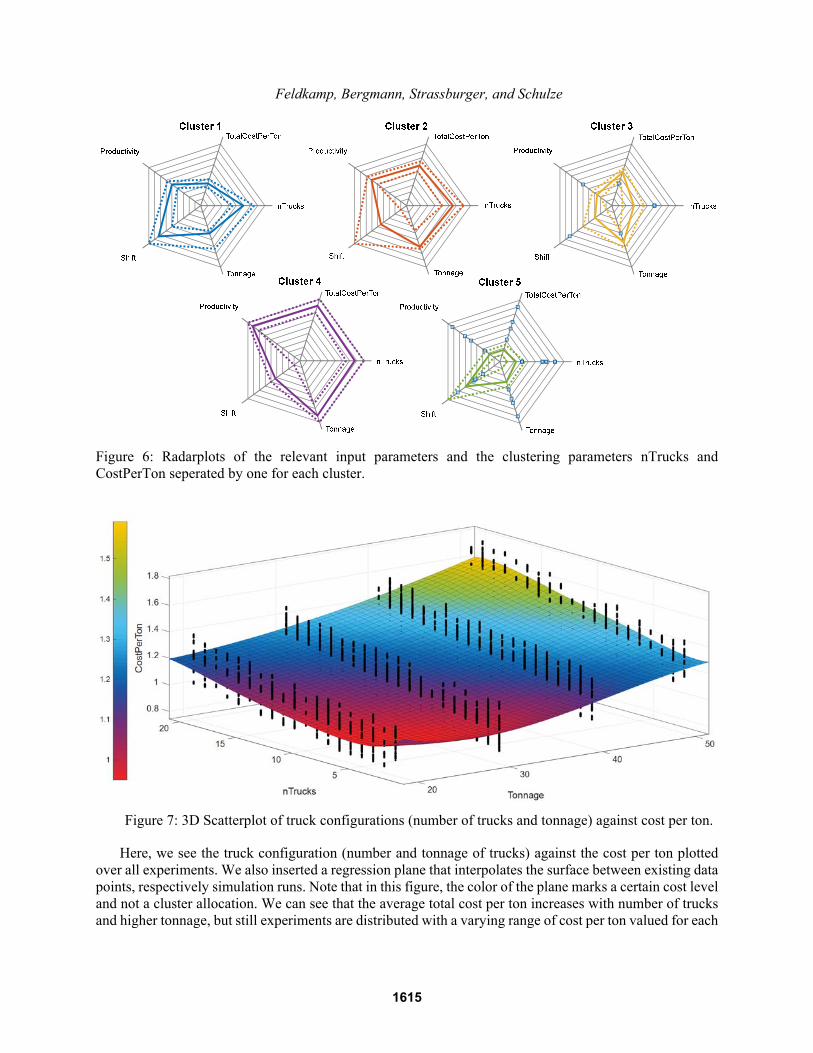
payload (Tonnage) are the most contributing parameters to the variance of Productivity. For the explanation of Cost per Ton, we also have to take the shift length into account. After identifying those parameters as most relevant, we investigate their distribution among each distinct cluster in a radar plot, which can be seen in Figure 6.

The plots in this figure mark the median and quartiles for each parameter. In between the quartiles lay 50% of all observations or simulation runs to be precise. So if quartiles lay close together, the corresponding parameter value is dominant in the given cluster.

From the blue cluster, which fits our target criteria best, we can derive that a shift regime with a high shift length, and medium number of trucks and tonnage is dominant and therefore leads to this cluster allocation. Furthermore, we can validate our assumption that the shift length has a stronger effect on the cost per ton than on the actual production output by looking at the radar plot for the purple cluster. This cluster has maximum productivity with a high number of trucks and maximum tonnage, but a shift regime with a medium (10 hours) shift length. Figure 7 illustrates this effect even more.

Linear Regression Model for Productivity Linear Regression Model for Cost per Ton

Estimate SE tStat tStat% pValue Estimate SE tStat tStat% pValue

(Intercept) ‐7660.36 58.304 ‐131.39 0 1.788 0.0024 758.21 0

nTrucks 313.77 0.673 466.51 54% 0 0.015 0.0000 558.05 24% 0

Tonnage 98.97 0.386 256.19 30% 0 0.013 0.0000 812.00 35% 0

SpeedDown 96.31 2.137 45.07 5% 0 ‐0.028 0.0001 ‐324.50 14% 0

LoadingTime ‐8.08 4.275 ‐1.89 0% 0 0.009 0.0002 52.85 2% 0

Shift 372.47 4.542 82.00 10% 0 ‐0.095 0.0002 ‐518.15 22% 0

WorkshopRate ‐8.36 1.173 ‐7.13 1% 0 0.002 0.0000 48.42 2% 0

1614


Figure 6: Radarplots of the relevant input parameters and the clustering parameters nTrucks and CostPerTon seperated by one for each cluster.

Figure 7: 3D Scatterplot of truck configurations (number of trucks and tonnage) against cost per ton.

Here, we see the truck configuration (number and tonnage of trucks) against the cost per ton plotted over all experiments. We also inserted a regression plane that interpolates the surface between existing data points, respectively simulation runs. Note that in this figure, the color of the plane marks a certain cost level and not a cluster allocation. We can see that the average total cost per ton increases with number of trucks and higher tonnage, but still experiments are distributed with a varying range of cost per ton valued for each

1615


given nTrucks/tonnage combination. If we investigate those datasets in detail, we see that the reason for this effect is that the shift length value differs among those simulation runs.

To finally answer the question for an optimal truck configuration for our base level loading point, we investigated the parameter values of our target cluster (the blue one) in detail through boxplots and histogram analysis and found out that in fact the dominating truck configuration in this cluster is between 10 and 16 trucks with 30t payload and a 11h shift regime. Conducting an new set of experiments for validating and optimizing those numbers is advisable when plans for reopening the mine become more specific.

4.3 Analysis Process for Sub-Question 3: Investigating Deeper Loading Ports

Part of our investigation is also the distribution of output parameters against the depth of the loading port, and also an investigation of how a good base level truck configuration performs if decision makers really decide to exploit deeper loading levels.

Figure 8: Target truck configuration against different Loading Levels.

Figure 8 shows exemplarily the shifting in productivity and cost per ton over a selection of loading levels. The depth of the loading port narrows the maximum reachable productivity regardless of truck configuration, and also a doubling of average total cost per ton from base level loading port to the deepest loading port on 2000 meters below surface. In order to investigate how our suggested truck configuration performs on different loading levels, we marked corresponding experiments in orange color. At loading port 1100 and 1200, this configuration hits the maximum target productivity. On deeper loading ports, we can simply add more trucks of the same tonnage to our portfolio to reach the target productivity (blue color). Note that a homogenous truck pool is the preferred solution for decision makers in this case study. From loading ports deeper than 1800 meters below surface, even the maximum number of 30t trucks is not able to reach the productivity goal, so bigger trucks with a heavier payload become necessary with a drastically increase in cost per ton.

5 SUMMARY AND FUTURE WORK

We successfully showed how to apply a knowledge discovery process onto a real world simulation model. General knowledge was created regarding waiting times of haul trucks and how cost per ton and

1616


productivity parameters are related to each other. Interestingly, the length of the shift regime does have a greater impact on the cost per ton progression than it does have on the output quantity of material. In terms of haul truck configuration, big trucks with maximum payload do not provide a good solution at the base level loading port, because they are dominated in cost per ton by lighter trucks. We recommend a 30t payload truck portfolio and showed how this configuration remains stable on deeper loading ports by simply adding more trucks of the same kind. Nevertheless, very deep loading levels bear a drastic increase of costs because target productivity can solely be reached with costly 50t payload trucks. Therefore it is questionable if exploiting loading levels deeper than 1800m below surface is profitable at all and is deepened on an appropriate gold price that needs to remain stable for a decent amount of time.

The knowledge created with our method guidelines a certain path, so future work should perform a more detailed simulation based optimization of our findings when plans for re-opening the mine are enacted. Regarding the outlined knowledge discovery process, we currently investigate a broader portfolio of suitable data mining algorithms and also we continue to further automate the knowledge discovery process to make it more end user friendly.

6 REFERENCES

Fayyad, U. M., G. Piatetsky-Shapiro, and P. Smyth. 1996. "From Data Mining to Knowledge Discovery in Databases." AI Magazine 17:37–54.

Feldkamp, N., S. Bergmann, and S. Strassburger. 2015a. "Knowledge Discovery in Manufacturing Simulations." In Proceedings of the 2015 ACM SIGSIM PADS Conference, 3–12.

Feldkamp, N., S. Bergmann, and S. Strassburger. 2015b. "Visual Analytics of Manufacturing Simulation Data." In Proceedings of the 2015 Winter Simulation Conference, edited by L. Yilmaz, W. K. V. Chan, I. Moon, T. M. K. Roeder, C. Macal, and M. D. Rossetti, 779–790. Piscataway, New Jersey: Institute of Electrical and Electronics Engineers, Inc.

Feldkamp, N., S. Bergmann, and S. Strassburger. 2016. "Innovative Analyse- und Visualisierungsmethoden für Simulationsdaten." In Multikonferenz Wirtschaftsinformatik (MKWI) 2016, edited by V. Nissen, et al., 1737–1748, Ilmenau: TU Ilmenau Universitätsbibliothek.

Henriksen, J. O. 1999. "SLX - The X is for eXtensibility." In Proceedings of the 1999 Winter Simulation Conference, edited by P. A. Farrington, H. B. Nembhard, D. T. Sturrock, and G. W. Evans, 167–175. Piscataway, New Jersey: Institute of Electrical and Electronics Engineers, Inc.

Kallfass, D., and T. Schlaak. 2012. "NATO MSG-088 Case Study Results to Demonstrate the Benefit of Using Data Farming for Military Decision Support." In Proceedings of the 2012 Winter Simulation Conference, edited by C. Laroque, J. Himmelspach, R. Pasupathy, O. Rose, and A. Uhrmacher, 1–12. Piscataway, New Jersey: Institute of Electrical and Electronics Engineers, Inc.

Keim, D. A., F. Mansmann, J. Schneidewind, J. Thomas, and H. Ziegler. 2008. "Visual Analytics: Scope and Challenges." In Visual Data Mining: Theory, Techniques and Tools for Visual Analytics, edited by S. Simoff, et al., Berlin, Heidelberg: Springer.

Kleijnen, J. P., S. M. Sanchez, T. W. Lucas, and T. M. Cioppa. 2005. "State-of-the-Art Review: A User’s Guide to the Brave New World of Designing Simulation Experiments." INFORMS Journal on Computing 17:263–289.

Law, A. M. 2014, Simulation Modeling and Analysis, 5th edn., McGraw Hill Book Co: New York, N.Y. Matkovic, K., D. Gracanin, M. Jelović, and H. Hauser. 2015. "Interactive Visual Analysis of Large

Simulation Ensembles." In Proceedings of the 2015 Winter Simulation Conference, edited by L. Yilmaz, W. K. V. Chan, I. Moon, T. M. K. Roeder, C. Macal, and M. D. Rossetti, 779–790. Piscataway, New Jersey: Institute of Electrical and Electronics Engineers, Inc.

MongoDB Inc. 2010. "Why Schemaless?" Accessed April 11, 2016. http://blog.mongodb.org/post/119945109/why-schemaless.

Sanchez, S. M. 2007. "Work Smarter, Not Harder: Guidelines for Designing Simulation Experiments." In Proceedings of the 2007 Winter Simulation Conference, edited by S. G. Henderson, S. G., B. Biller,

1617

Feldkamp, Bergmann, Strassburger, and Schulze M.-H. Hsieh, J. Shortle, J. D. Tew, and R. R. Barton, 84–94. Piscataway, New Jersey: Institute of Electrical and Electronics Engineers, Inc.

Sanchez, S. M. 2014. "Simulation Experiments: Better Data, Not Just Big Data." In Proceedings of the 2014 Winter Simulation Conference, edited by A. Tolk, S. D. Diallo, I. O. Ryzhov, L. Yilmaz, S. Buckley, and J. A. Miller, 805–816. Piscataway, New Jersey: Institute of Electrical and Electronics Engineers, Inc.

Sanchez, S. M., and H. Wan. 2009. "Better than a Petaflop: The Power of Efficient Experimental Design." In Proceedings of the 2009 Winter Simulation Conference (WSC 2009), edited by M. D. Rossetti, R. R. Hill, B. Johansson, Dunkin A., and R. G. Ingalls, 60–74. Piscataway, New Jersey: IEEE.

Theodoropoulos, G. 2015. "Simulation in the Era of Big Data: Trends and Challenges." In Proceedings of the 3rd ACM SIGSIM Conference on Principles of Advanced Discrete Simulation, 1, New York, NY, USA: ACM.

Thomas, J. J., and K. A. Cook. 2005, Illuminating the Path. Research and Development Agenda for Visual Analytics, IEEE Computer Society: Los Alamitos, California.

Vieira, H., S. M. Sanchez, K. H. Kienitz, and M. C. N. Belderrain. 2011. "Improved Efficient, Nearly Orthogonal, Nearly Balanced Mixed Designs." In Proceedings of the 2011 Winter Simulation Conference (WSC 2011), edited by S. Jain, R. Creasey, J. Himmelspach, K. P. White, and M. C. Fu, 3600–3611. Piscataway, New Jersey: Institute of Electrical and Electronics Engineers, Inc.

AUTHOR BIOGRAPHIES

NICLAS FELDKAMP holds bachelor and master degrees in business information systems from the University of Cologne and the Ilmenau University of Technology, respectively. He is currently working as a doctoral student at the Department of Industrial Information Systems of the Ilmenau University of Technology. His research interests include data science, business analytics, and industrial simulations. His email address is [email protected]. SÖREN BERGMANN holds a Doctoral and Diploma degree in business information systems from the Ilmenau University of Technology. He is a member of the scientific staff at the Department for Industrial Information Systems. Previously he worked as corporate consultant in various projects. His research interests include generation of simulation models and automated validation of simulation models within the digital factory context. His email is [email protected]. STEFFEN STRASSBURGER is a professor at the Ilmenau University of Technology and head of the Department for Industrial Information Systems. Previously he was head of the “Virtual Development” department at the Fraunhofer Institute in Magdeburg, Germany and a researcher at the DaimlerChrysler Research Center in Ulm, Germany. He holds a Doctoral and a Diploma degree in Computer Science from the University of Magdeburg, Germany. He is further an associate editor of the Journal of Simulation. His research interests include distributed simulation, automatic simulation model generation, and general interoperability topics within the digital factory context. He is also an active member of the Simulation Interoperability Standards Organization (SISO). His web page can be found via http://www.tu-ilmenau.de/wi1. His email is [email protected]. THOMAS SCHULZE is a professor in the School of Computer Science at the Otto-von-Guericke-University, Magdeburg, Germany. He received the Ph.D. degree in civil engineering in 1979 and his habil. Degree for computer science in 1991 from the University of Magdeburg. His research interests include modeling methodology, manufacturing simulation, distributed simulation with HLA and visualization. He is an active member in the ASIM, the German organization of simulation. His email address is [email protected].

1618

proceedings of the 2016 winter simulation conference t. m

Documents