proc. of the 18th python in science conf. (scipy …proc. of the 18th python in science conf. (scipy...
TRANSCRIPT
PROC OF THE 18th PYTHON IN SCIENCE CONF (SCIPY 2019) 1
PyDDA A new Pythonic Wind Retrieval Package
Robert JacksonDaggerlowast Scott CollisDagger Timothy Langsect Corey Potvinpara Todd MunsonDagger
F
AbstractmdashPyDDA is a new community framework aimed at wind retrievals thatdepends only upon utilities in the SciPy ecosystem such as scipy numpy anddask It can support retrievals of winds using information from weather radarnetworks constrained by high resolution forecast models over grids that coverthousands of kilometers at kilometer-scale resolution Unlike past wind retrievalpackages this package can be installed using anaconda for easy installationand with a focus on ease of use can retrieve winds from gridded radar andmodel data with just a few lines of code The package is currently available fordownload at httpsgithubcomopenradarPyDDA
Index Termsmdashwind retrieval hurricane tornado radar
Introduction
Three dimensional wind retrievals are important for examiningthe dynamics that drive severe weather such as tornadoes andhurricanes In addition spatial wind retrievals inside severe con-vection are important for assessing the wind damage they causeScanning radars provide the best opportunity for providing threedimensional volumes of winds inside severe weather Howeverthe retrieval of three dimensional winds from weather radars isa nontrivial task Given that the radar measures the speed ofscatterers in the direction of the radar beam rather than the fullwind velocity retrieving these winds requires more informationthan the Doppler velocities measured by a single weather radarTypically the 3D wind field is retrieved based on constraints withregards to physical laws such as conservation of mass or wind datafrom other sources such as model reanalyses wind profilers andrawinsondes In particular atmospheric scientists use two methodsto retrieve winds from scanning weather radars The first methodprescribes a strong constraint on the wind field according to themass continuity equation The second method is a variationaltechnique that places weak constraints on the wind field by findingthe wind field that minimizes a cost function according to deviancefrom physical laws or from observations ([SPG09] [PSX12])
Currently existing software for wind retrievals includes soft-ware based off of the strong constraint technique such as CEDRIC[MF98] as well as software based off of the weak variationaltechnique such as MultiDop [LSKJ17] Since CEDRIC uses astrong constraint from mass continuity equation to retrieve winds
Corresponding author rjacksonanlgovDagger Argonne National Laboratory Argonne IL USAsect NASA Marshall Space Flight Center Huntsville AL USApara NOAAOAR National Severe Storms Laboratory Norman OK USA|| School of Meteorology University of Oklahoma Norman OK USA
Copyright copy 2019 Robert Jackson et al This is an open-access article dis-tributed under the terms of the Creative Commons Attribution License whichpermits unrestricted use distribution and reproduction in any medium pro-vided the original author and source are credited
the addition of constraints from other data sources is not possiblewith CEDRIC Also while CEDRIC was revolutionary for itstime it is difficult to use as a separate scripting language is theinput for the retrieval While MultiDop is based off of the morecustomizable 3D variational technique it is fixed to 2 or 3 radarsand is not scalable Also Multidop does not support the addition of3D wind fields from models or other retrievals Finally Multidopis a wrapper around a program written in C which introducesissues related to packaging and scalability due to the non-thread-safe nature of the wrapper
The limitations in current wind retrieval software moti-vated development of Pythonic Direct Data Assimilation (Py-DDA)PyDDA is currently available for download at httpsopenradarscienceorgPyDDA PyDDA is entirely written inPython and uses only tools in the Scientific Python ecosystem suchas NumPy [vdWCV11] SciPy [JOP+01] and Cartopy [Off15]This therefore permits the easy installation of PyDDA using pipor anaconda Given that installation is a major hurdle to usingcurrently existing retrieval software this makes it easier for thosewho are not radar scientists to be able to use the software Unlikecurrently existing software a suite of unit tests are built intoPyDDA that are executed whenever a user make a contribution toPyDDA ensuring that the package will function for the user Withregards to ease of use PyDDA can retrieve winds from multipleradars combined with data from model reanalyses with just a fewlines of code In addition PyDDA is built upon the Python ARMRadar Toolkit (Py-ART) [HC16] Since Py-ART is already usedby hundreds of users in the radar meteorology community theseusers would be able to learn how to use PyDDA easily Moreoverthe open source nature of PyDDA encourages contributions byusers for further enhancement In essence PyDDA was createdwith a goal in mind to make radar wind retrievals more accessibleto the scientific community through both ease of installation anduse
This paper will first show the implementation of the variationaltechnique used in PyDDA After that this paper shows examplesof retrieving and visualizing gridded radar data with PyDDAFinally several use cases in severe convection such as HurricaneFlorence and a tornado in Sydney Australia are shown in orderto provide examples on how this software can be used by thoseinterested in validating severe weather forecasts and assessingwind damage
Three dimensional variational (3DVAR) technique
The wind retrieval used by PyDDA is the three dimensionalvariational technique (3DVAR) 3DVAR retrieves winds by findingthe wind vector field ~V that minimizes the cost function J(V) This
httpsntrsnasagovsearchjspR=20190027316 2020-03-30T130603+0000Z
2 PROC OF THE 18th PYTHON IN SCIENCE CONF (SCIPY 2019)
Cost function Basis of constraint
Jo(~V) Radar observationsJc(~V) Mass continuity equationJv(~V) Vertical vorticity equationJm(~V) Model field constraintJb(~V) Background constraint (raw-
insonde data)Js(~V) Smoothness constraint
TABLE 1 List of cost functions implemented in PyDDA
cost function is the weighted sum of many different cost functionsrelated to various constraints The detailed formulas behind thesecost functions can be found in [SPG09] [PSX12] as well as in thesource code of the cost_functions module of PyDDA Thedetails behind constructing the model constraint are provided inthe next section
The cost function ~V is then typically expressed as
J(~V) = Jo(~V)+ Jc(~V)+ Jv(~V)+ Jm(~V)+ Jb(~V)+ Js(~V)
where each addend is as in Table 1The evaluation of J(V) can be done entirely using calls from
NumPy and SciPy For example evaluating Jc(~V) = nabla middot~V with anoptional anelastic term be reduced to a few NumPy calls The codethat executes these NumPy calls can be found in the Appendix
Since NumPy can be configured to take advantage of opensource mathematics libraries that parallelize the calculation thisalso extends the capability of the retrieval to use the availablecores on the machine in addition to simplifying the code Each costfunction and its gradient can be expressed in an analytical formusing variational calculus so the addition of more cost functionsis possible due to the modular nature of each constraint
These calculations are then done in order to find the ~Vthat minimizes ~J(V) A common technique to minimize J(V)calculates
~Vn = ~Vnminus1minusα(nabla~V)
for an α gt 0 until there is convergence to a solution given thatan initial guess ~V0 is provided This is called the gradient descentmethod that finds the minimum by decrementing ~V in the directionof steepest descent along J Multidop uses a variant of the gradientdescent method the conjugate gradient descent method in orderto minimize the cost function ~J(V)
However convergence can be slow for certain cost func-tions Therefore in order to ensure faster convergence PyDDAuses the limited memory BroydenndashFletcherndashGoldfarbndashShanno (L-BGFS) technique that optimizes the gradient descent method byapproximating the Hessian from previous iterations The inverseof the approximate Hessian is then used to find the optimal searchdirection and α for each retrieval [BLNZ95] Since there arephysically realistic constraints to ~V the L-BFGS box (L-BFGS-B) variant of this technique can take advantage of this by onlyusing L-BFGS on what the algorithm identifies as free variablesoptimizing the retrieval further In PyDDA we constrain thesolution to ensure that each individual component of ~V is within arange of (minus100 m sminus1100 m sminus1)
The L-BFGS-B algorithm is implemented in SciPy Afterthe initial wind field is provided PyDDA calls 10 iterations ofL-BFGS-B using scipyoptimizefmin_l_bfgs_b Py-DDA will then then test for convergence of a solution by either
Data source Routine in initialization module
WeatherResearch andForecasting(WRF)
make_background_from_wrf
High ResolutionRapid Refresh(HRRR)
make_initialization_from_hrrr
ERA Interim make_initialization_from_era_interim
Rawinsonde make_wind_field_from_profile
Constant field make_constant_wind_field
TABLE 2 The differing initializations PyDDA can provide to theuser These initializations are constructed by interpolating the modelJ(~V) to the analysis grid coordinates
detecting whether the maximum change in vertical velocity be-tween the current solution and the previous 10 iterations is lessthan 002 m sminus1 or if
∥∥∥~V∥∥∥lt 10minus3 signifying that we have reached
a local minimum in ~V In addition in order to reduce noise in theretrieved ~V there are options for the user to use a low pass filteron the retrieval as well as to adjust the smoothness constraint
Executing the 3DVAR technique with just a few lines of code
With one line of code one can use the3DVAR technique to retrieve winds using thepyddaretrievalget_dd_wind_field procedureIf one has a list of Py-ART grids list_of_grids that theyhave loaded and provide ~V0 into arrays called u_init v_initand w_init retrieval of winds is as easy aswinds = pyddaretrievalget_dd_wind_field(
list_of_grids ui vi wi)
PyDDA even includes an initialization module that will generateexample ui vi and wi for the user For example in order togenerate a simple initial wind field of ~V =~0 in the shape of anyone of the grids in list_of_grids simply doimport pyddainitialization as init
ui vi wi = initmake_constant_wind_field(list_of_grids[0] wind=(00 00 00))
The user can add their own custom con-straints and initializations into PyDDA Sincepyddaretrievalget_dd_wind_field has 3D NumPyarrays as inputs for the initialization this allows the user to enterin an arbitrary NumPy array with the same shape as the analysisgrid as the initialization field
In addition PyDDA includes four different initialization rou-tines that will create this field for you from various data sourcessuch as ERA-Interim Similar to when the constraints are createdthe initialization is created by interpolating the original model datafrom its coordinates to the analysis grid coordinates using nearest-neighbor interpolation This initialization is then entered in as ~V0in the optimization loop
A similar set of routines exist in in the constraintsmodulefor creating constraints from model fields These routines arelisted in Table 3 In order to create these constraints PyDDAwill first interpolate the model wind field ~Vm from the datarsquosoriginal coordinates data into the analysis gridrsquos coordinates using
PYDDA A NEW PYTHONIC WIND RETRIEVAL PACKAGE 3
Data source Routine in constraints module
WeatherResearch andForecasting(WRF)
make_constraint_from_wrf
High ResolutionRapid Refresh(HRRR)
add_hrrr_constraint_to_grid
ERA Interim make_constraint_from_era_interim
TABLE 3 The differing model constraints PyDDA can provide tothe user These constraints are constructed by interpolating the modelJ(~V) to the analysis grid coordinates
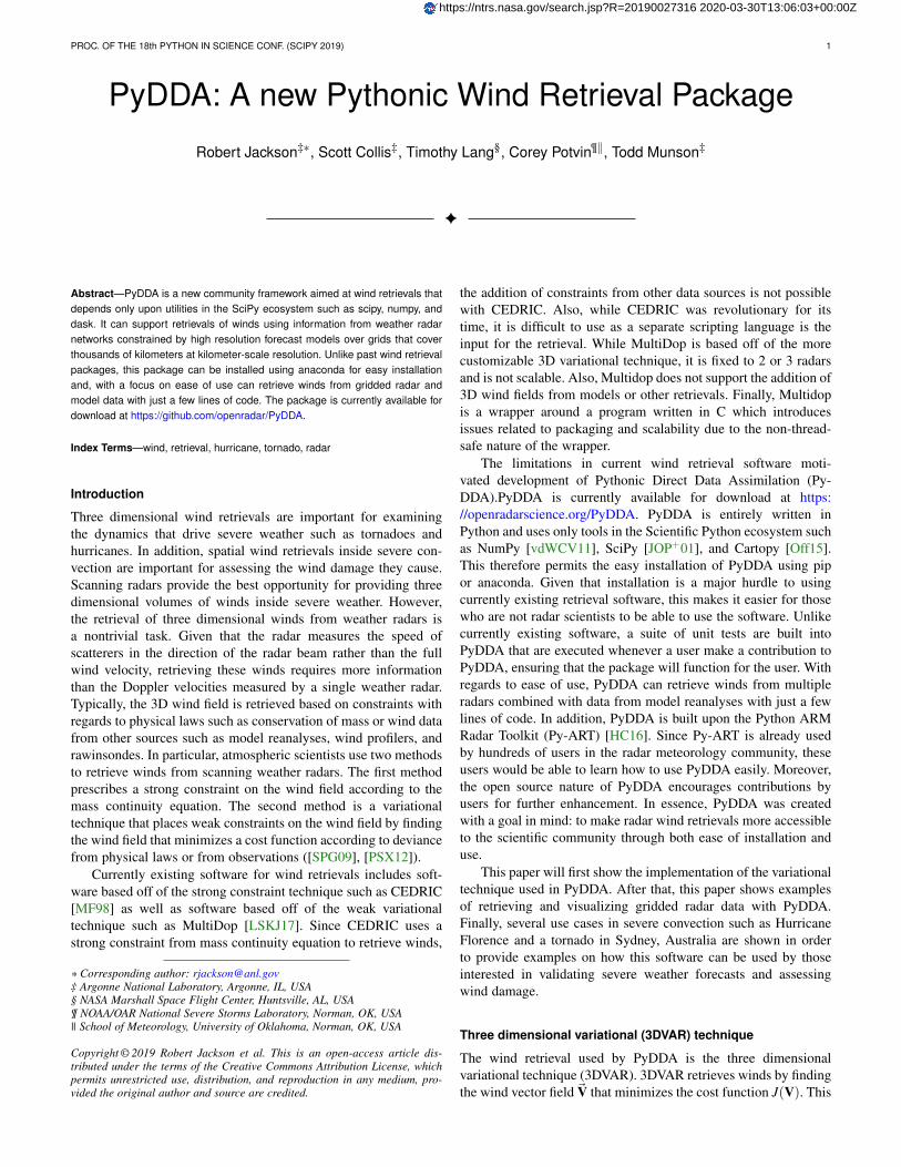
Fig 1 An example streamline plot of winds in Hurricane Florenceoverlaid over radar estimated rainfall rate The LKTX and KMHXNEXt Generation Radars (NEXRADs) were used to retrieve the windsand rainfall rates The blue contour represents the region containinggale force winds while the red contour represents the regions wherehurricane force winds are present
nearest-neighbor interpolation After that for each model an extraterm is added to J(~V) in the optimization technique This termcorresponds to the sum of the squared error between the ~V and~Vm
Jm(~V) = cm sum(i jk) isin domain
(vi jkminus vmi jk)2
cm is the weight given to this constraint by the user The codesnippet below will interpolate an HRRR model run to a Py-ARTgrid called mygrid The get_dd_wind_field will then lookfor the name of the model inside mygridwhen calculating Jm(~V)import pyddaconstraints as const
Add HRRR GRIB filehrrr_path = my_hrrr_filegribmygrid = constadd_hrrr_constraint_to_grid(
mygrid hrrr_path)
The model constraints and retrieval initializations are based off ofany 3D field with the same array size and grid specification asthe input radar grids Therefore these lists can be easily expandedwith user routines that interpolate the model or other observationaldata to the analysis grid
Visualization module
In addition PyDDA also supports 3 types of basic visualizationswind barb plots quiver plots and streamline plots These plotsare created using matplotlib and return a matplotlib axis handle so
that the user can use matplotlib to make further customizations tothe plots For example creating a plot of winds on a geographicalmap with contours overlaid on it such as what is shown in Figure1 is as simple as
import pyartimport pyddaimport cartopycrs as ccrs
Load Gridsltx_grid = pyartioread_grid(ltx_gridnc)mhx_grid = pyartioread_grid(mtx_gridnc)
Set up projection and plot of windsax = pltaxes(projection=ccrsPlateCarree())ax = pyddavisplot_horiz_xsection_streamlines_map(
[ltx_grid mhx_grid] ax=axbackground_field=rainfall_rate bg_grid_no=-1level=2 vmin=0 vmax=50 show_lobes=False)
You can add more layers of data that you wishwind_speed = npsqrt(ltx_gridfields[u][data]2wind_speed += ltx_gridfields[v][data]2)wind_speed = wind_speedfilled(npnan)lons = ltx_gridpoint_longitude[data]lats = ltx_gridpoint_latitude[data]cs = axcontour(
lons[2] lats[2] wind_speed[2] levels=[28 32]linewidths=8 colors=[b r k])
pltclabel(cs ax=ax inline=1 fontsize=15)
Adjust axes propertiesaxset_xticks(nparange(-80 -75 05))axset_yticks(nparange(33 358 05))axset_title(ltx_gridtime[units][-20])
This therefore makes it very easy to create quicklook plotsfrom the data In addition to horizontal cross sections PyDDAcan also plot wind cross sections in the x-z and y-z planes sothat one can view a vertical cross section of winds Since thepyddavisplot_horiz_xsection_streamlines_mapreturns a matplotlib axes handle it is then possible for the user tocustomize the plot further to add features such as wind contoursas well as adjust the axes limits as shown in the code above
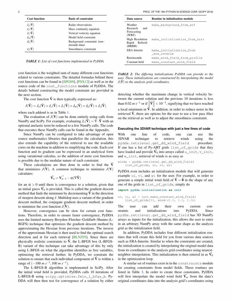
In addition to streamline plots PyDDA also supports visual-ization through quiver plots Creating a quiver plot from a datasetthat looks like Figure 2 in this case a single Doppler retrieval isas easy as
import pyartimport pydda
Grids = [pyartioread_grid(mywindsnc)]pltfigure(figsize=(77))pyddavisplot_horiz_xsection_quiver(
Grids None reflectivity level=6quiver_spacing_x_km=100quiver_spacing_y_km=100)
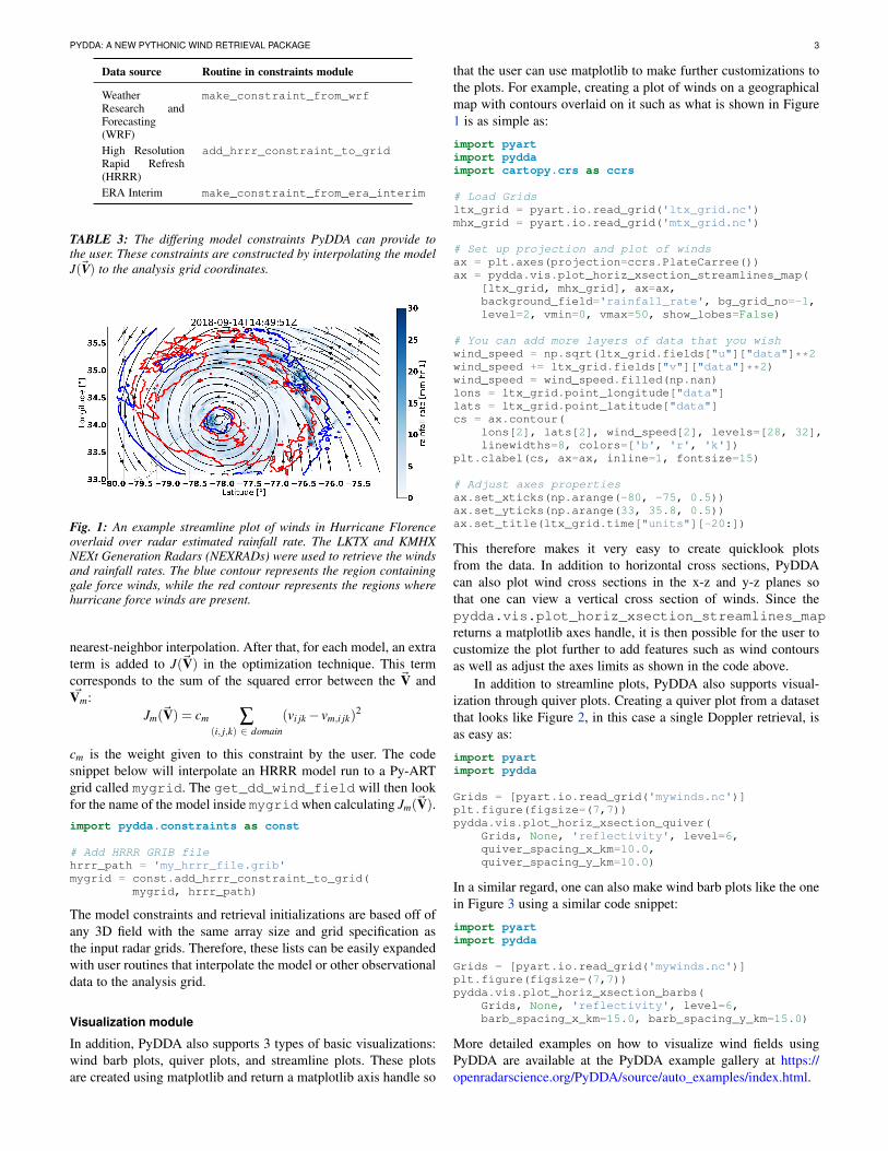
In a similar regard one can also make wind barb plots like the onein Figure 3 using a similar code snippet
import pyartimport pydda
Grids = [pyartioread_grid(mywindsnc)]pltfigure(figsize=(77))pyddavisplot_horiz_xsection_barbs(
Grids None reflectivity level=6barb_spacing_x_km=150 barb_spacing_y_km=150)
More detailed examples on how to visualize wind fields usingPyDDA are available at the PyDDA example gallery at httpsopenradarscienceorgPyDDAsourceauto_examplesindexhtml
4 PROC OF THE 18th PYTHON IN SCIENCE CONF (SCIPY 2019)
Fig 2 An example wind quiver plot from a retrieval from the C-band Polarization Radar Berrimah radar and a weather balloon overDarwin on 20 Jan 2006 The background colors represent the radarreflectivity
Fig 3 As Figure 2 but using wind barbs
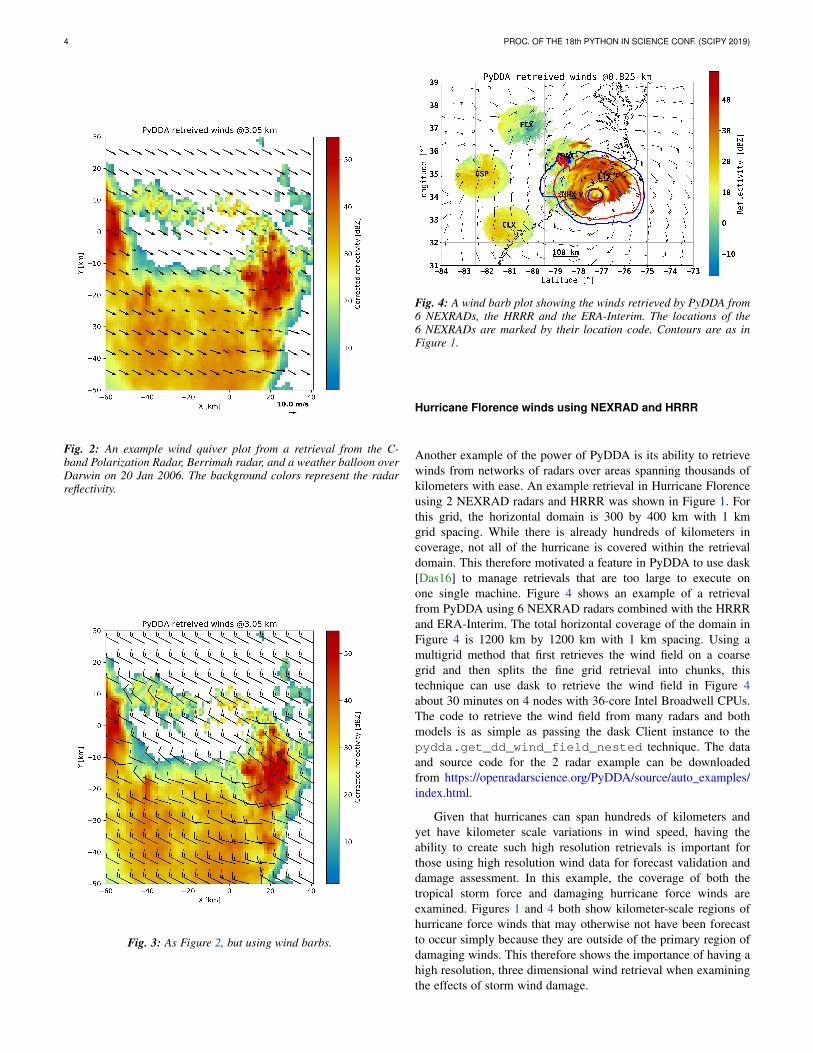
Fig 4 A wind barb plot showing the winds retrieved by PyDDA from6 NEXRADs the HRRR and the ERA-Interim The locations of the6 NEXRADs are marked by their location code Contours are as inFigure 1
Hurricane Florence winds using NEXRAD and HRRR
Another example of the power of PyDDA is its ability to retrievewinds from networks of radars over areas spanning thousands ofkilometers with ease An example retrieval in Hurricane Florenceusing 2 NEXRAD radars and HRRR was shown in Figure 1 Forthis grid the horizontal domain is 300 by 400 km with 1 kmgrid spacing While there is already hundreds of kilometers incoverage not all of the hurricane is covered within the retrievaldomain This therefore motivated a feature in PyDDA to use dask[Das16] to manage retrievals that are too large to execute onone single machine Figure 4 shows an example of a retrievalfrom PyDDA using 6 NEXRAD radars combined with the HRRRand ERA-Interim The total horizontal coverage of the domain inFigure 4 is 1200 km by 1200 km with 1 km spacing Using amultigrid method that first retrieves the wind field on a coarsegrid and then splits the fine grid retrieval into chunks thistechnique can use dask to retrieve the wind field in Figure 4about 30 minutes on 4 nodes with 36-core Intel Broadwell CPUsThe code to retrieve the wind field from many radars and bothmodels is as simple as passing the dask Client instance to thepyddaget_dd_wind_field_nested technique The dataand source code for the 2 radar example can be downloadedfrom httpsopenradarscienceorgPyDDAsourceauto_examplesindexhtml
Given that hurricanes can span hundreds of kilometers andyet have kilometer scale variations in wind speed having theability to create such high resolution retrievals is important forthose using high resolution wind data for forecast validation anddamage assessment In this example the coverage of both thetropical storm force and damaging hurricane force winds areexamined Figures 1 and 4 both show kilometer-scale regions ofhurricane force winds that may otherwise not have been forecastto occur simply because they are outside of the primary region ofdamaging winds This therefore shows the importance of having ahigh resolution three dimensional wind retrieval when examiningthe effects of storm wind damage
PYDDA A NEW PYTHONIC WIND RETRIEVAL PACKAGE 5
Fig 5 The locations of the four operational radars operated by theBureau of Meteorology in the vicinity of Sydney Australia The circlesrepresent the maximum unambiguous range of each radar
Fig 6 A quiver plot inside a supercell that spawned a tornado inthe vicinity of Sydney Australia The area inside the hatched contourrepresents regions where the updraft velocity is greater than 1 ms tohighlight regions where updrafts are present
Tornado in Sydney Australia using 4 radars
In addition to retrieving winds in hurricanes PyDDA can alsointegrate data from radar networks in order to retrieve the windsinside tornadoes For example a network of four scanning radarsin the vicinity of Sydney Australia captured a supercell withinthe vicinity of Sydney as shown in Figure 5 In this retrieval ahorizontal domain of 350 km by 550 km with 1 km grid spacingwas used
Figure 6 shows the winds retrieved by PyDDA inside thissupercell Using data from the radars PyDDA is able to providea complete picture of the rotation inside the supercell and evenresolves the updraft in the vicinty of the mesocyclone Suchdatasets can be of use for estimating the winds inside a tornadoat altitudes as low as 500 m above ground level This therefore
Fig 7 The locations of the two X-band Scanning Precipitation Radars(XSAPRs) I5 and I6 as well as the KVNX NEXRAD The two circlesrepresent the maximum unambiguous range of the XSAPR radars Themaximum unambiguous range of KVNX covers the entire figure
is capable of providing wind datasets that can be used to bothprovide an estimated wind speed for wind damage assessmentsas well as for verification of supercell simulations from weatherforecasting models The data and source code for this exampleis also available at httpsopenradarscienceorgPyDDAsourceauto_examplesindexhtml
Combining winds from 3 scanning radars with HRRR in Okla-homa
A final example shows how easily data from multiple radars andmodels can be combined together In this case we integrate datafrom three scanning radars whose locations are shown in Figure 7in the vicinity of the Atmospheric Radiation Measurement (ARM)Southern Great Plains (SGP) site In this example the 2 XSAPRradars are at X-band and therefore have lower coverage but greaterresolution than the S-band KVNX radar In addition the HighResolution Rapid Refresh was used as an additional constraintwith the constraint stronger in regions without radar coverageThe horizontal domain for the retrieval was 100 km by 100 kmwith 1 km spacing
Figure 8 shows the resulting wind field of such a retrievalduring a case of stratiform rain with embedded convection thatoccurred over the SGP site on 04 October 2017 Generallyweaker winds and a less organized structure is seen comparedto the previous two examples This would be expected in suchconditions However this also demonstrates the success in inte-grating radar data from 3 radars and a high resolution reanalysisto provide the most complete wind retrieval possible The dataand source code for this example is also available at httpsopenradarscienceorgPyDDAsourceauto_examplesindexhtml
Validation
PyDDA utilizes a series of unit tests in order to ensure thatquality results are produced with each build of PyDDAThese tests are implemented using pytest In total PyDDAcurrently has 27 tests on the software that test all aspectsof the software including the cost functions optimizationloop and visualizations For each pull request to the masterbranch of PyDDA Travis CI runs this suite of unit tests on
6 PROC OF THE 18th PYTHON IN SCIENCE CONF (SCIPY 2019)
Fig 8 A quiver plot of a wind retrieval from 2 XSAPR radars andthe KVNX NEXRAD radar in Oklahoma In addition the HRRR wasused as a constraint The wind barbs are plotted over the reflectivityderived from the maximum of the reflectivity from the 3 radars
the program in order to ensure functionality of the programExamples of unit tests that are executed by PyDDA are basedon expected results from theoretical considerations regardingeach cost function For example in order to evaluate whetherpyddacost_functionscalculate_mass_continuityis working correctly the tests evaluate this function using a windfield with surface convergence in the center If the cost function isnegative as would be expected then the unit test passes Anotherexample evaluates whether the model cost function is workingby checking to see if the wind field from the optimization loopconverges to the model input if no other data or constraints arespecified In addition the visualization modules are tested bycomparing their results against baseline images to ensure that theyare functioning correctly
Contributor Information
We are currently welcoming contributions from the communityinto PyDDA A PyDDA road map demonstrates what kinds ofcontributions to PyDDA would be useful As of the writing of thispaper the road map states that the current goals of PyDDA are toimplement
bull Support for a greater number of high resolution (LES)models such as CM1 [BF02]
bull Support for integrating in data from the Rapid Refreshbull Coarser resolution reanalyses such as the NCEP reanalysis
as initializations and constraintsbull Support for individual point analyses such as those from
wind profilers and METARsbull Support for radar data in antenna coordinatesbull Improvements in visualizations
bull Documentation improvements including better descrip-tions in the current English version of the documentationand versions of the documentation in non-English lan-guages
All contributions to PyDDA will have to be submitted by apull request to the master branch on httpsgithubcomopenradarPyDDA From there the main developers will examine the pullrequest to see if unit tests are needed and if the contribution bothhelps contribute to the goals of the road map and if it passes asuite of unit tests in order to ensure the functionality of PyDDAIn addition we also require that the user provide documentationfor the code they contribute For the full information on howto make a contribution go to the contributorrsquos guide at httpsopenradarscienceorgPyDDAcontributors_guideindexhtml
In addition for further information about how to use PyDDAplease consult the documentation at httpsopenradarscienceorgPyDDA
Acknowledgments
The HRRR data were downloaded from the University of Utaharchive [BHL17] In addition the authors would like to thankAlain Protat for providing the Sydney tornado wind data PyDDAwas partially supported by the Climate Model Development andValidation Activity of the Department of Energy Office of ScienceDr Tsengdar Lee of the NASA Weather program provided fundsthat supported the development of MultiDop a critical intermedi-ate step toward the development of PyDDA
Appendix Mass continuity cost function in Python
This appendix shows an example cost function from PyDDA Thecode snippet below shows how the mass continuity cost functioncan be implemented using NumPyimport numpy as np
def calculate_mass_continuity(u v w z dx dy dz coeff=15000 anel=1)Calculates the mass continuity cost function bytaking the divergenceof the wind field
All arrays in the given lists must have the samedimensions and represent the same spatialcoordinates
Parameters----------u Float array
Float array with u component of wind fieldv Float array
Float array with v component of wind fieldw Float array
Float array with w component of wind fielddx float
Grid spacing in x directiondy float
Grid spacing in y directiondz float
Grid spacing in z directionz Float array (1D)
1D Float array with heights of gridcoeff float
Constant controlling contribution of masscontinuity to cost function
anel int= 1 use anelastic approximation 0=dont
PYDDA A NEW PYTHONIC WIND RETRIEVAL PACKAGE 7
Returns-------J float
value of mass continuity cost functiondudx = npgradient(u dx axis=2)dvdy = npgradient(v dy axis=1)dwdz = npgradient(w dz axis=0)
if(anel == 1)rho = npexp(-z100000)drho_dz = npgradient(rho dz axis=0)anel = wrhodrho_dz
elseanel = npzeros(wshape)
return coeffnpsum(npsquare(dudx + dvdy + dwdz + anel))20
REFERENCES
[BF02] George H Bryan and J Michael Fritsch A benchmarksimulation for moist nonhydrostatic numerical modelsMonthly Weather Review 130(12)2917ndash2928 2002 URLhttpsdoiorg1011751520-0493(2002)130lt2917ABSFMNgt20CO2 arXivhttpsdoiorg1011751520-0493(2002)130lt2917ABSFMNgt20CO2doi1011751520-0493(2002)130lt2917ABSFMNgt20CO2
[BHL17] Brian K Blaylock John D Horel and Samuel T Liston Cloudarchiving and data mining of high-resolution rapid refresh fore-cast model output Computers and Geosciences 10943 ndash 502017 URL httpwwwsciencedirectcomsciencearticlepiiS0098300417305083 doihttpsdoiorg101016jcageo201708005
[BLNZ95] Richard H Byrd Peihuang Lu Jorge Nocedal and Ciyou ZhuA limited memory algorithm for bound constrained optimizationSIAM J Sci Comput 16(5)1190ndash1208 September 1995 URLhttpdxdoiorg1011370916069 doi1011370916069
[Das16] Dask Development Team Dask Library for dynamic taskscheduling 2016 URL httpdaskpydataorg
[HC16] Jonathan Helmus and Scott Collis The Python ARMRadar Toolkit (Py-ART) a Library for Working withWeather Radar Data in the Python Programming Lan-guage Journal of Open Research Software 4(1) July 2016URL httpopenresearchsoftwaremetajnlcomarticles105334jors119 doi105334jors119
[JOP+01] Eric Jones Travis Oliphant Pearu Peterson et al Scipy Opensource scientific tools for python 2001 [Online accessedlttodaygt] URL httpwwwscipyorg
[LSKJ17] Timothy Lang Mario Souto Shahin Khobahi and Bobby Jack-son nasamultidop Multidop v03 October 2017 URL httpsdoiorg105281zenodo1035904 doi105281zenodo1035904
[MF98] L Jay Miller and Sherrie M Fredrick Custom editing anddisplay of reduced information in cartesian space (cedric) man-ual Technical report National Center for Atmospheric ResearchMesoscale and Microscale Meteorology Division Boulder CO1998
[Off15] Met Office Cartopy a cartographic python library with amatplotlib interface Exeter Devon 2010 - 2015 URLhttpscitoolsorgukcartopy
[PSX12] Corey K Potvin Alan Shapiro and Ming Xue Impactof a vertical vorticity constraint in variational dual-dopplerwind analysis Tests with real and simulated supercell dataJournal of Atmospheric and Oceanic Technology 29(1)32ndash49 2012 URL httpsdoiorg101175JTECH-D-11-000191 arXivhttpsdoiorg101175JTECH-D-11-000191 doi101175JTECH-D-11-000191
[SPG09] Alan Shapiro Corey K Potvin and Jidong Gao Useof a vertical vorticity equation in variational dual-doppler wind analysis Journal of Atmospheric andOceanic Technology 26(10)2089ndash2106 2009 URLhttpsdoiorg1011752009JTECHA12561 arXivhttpsdoiorg1011752009JTECHA12561doi1011752009JTECHA12561
[vdWCV11] S van der Walt S C Colbert and G Varoquaux Thenumpy array A structure for efficient numerical computationComputing in Science Engineering 13(2)22ndash30 March 2011doi101109MCSE201137
- Introduction
- Three dimensional variational (3DVAR) technique
- Executing the 3DVAR technique with just a few lines of code
- Visualization module
- Hurricane Florence winds using NEXRAD and HRRR
- Tornado in Sydney Australia using 4 radars
- Combining winds from 3 scanning radars with HRRR in Oklahoma
- Validation
- Contributor Information
- Acknowledgments
- Appendix Mass continuity cost function in Python
- References
-
2 PROC OF THE 18th PYTHON IN SCIENCE CONF (SCIPY 2019)
Cost function Basis of constraint
Jo(~V) Radar observationsJc(~V) Mass continuity equationJv(~V) Vertical vorticity equationJm(~V) Model field constraintJb(~V) Background constraint (raw-
insonde data)Js(~V) Smoothness constraint
TABLE 1 List of cost functions implemented in PyDDA
cost function is the weighted sum of many different cost functionsrelated to various constraints The detailed formulas behind thesecost functions can be found in [SPG09] [PSX12] as well as in thesource code of the cost_functions module of PyDDA Thedetails behind constructing the model constraint are provided inthe next section
The cost function ~V is then typically expressed as
J(~V) = Jo(~V)+ Jc(~V)+ Jv(~V)+ Jm(~V)+ Jb(~V)+ Js(~V)
where each addend is as in Table 1The evaluation of J(V) can be done entirely using calls from
NumPy and SciPy For example evaluating Jc(~V) = nabla middot~V with anoptional anelastic term be reduced to a few NumPy calls The codethat executes these NumPy calls can be found in the Appendix
Since NumPy can be configured to take advantage of opensource mathematics libraries that parallelize the calculation thisalso extends the capability of the retrieval to use the availablecores on the machine in addition to simplifying the code Each costfunction and its gradient can be expressed in an analytical formusing variational calculus so the addition of more cost functionsis possible due to the modular nature of each constraint
These calculations are then done in order to find the ~Vthat minimizes ~J(V) A common technique to minimize J(V)calculates
~Vn = ~Vnminus1minusα(nabla~V)
for an α gt 0 until there is convergence to a solution given thatan initial guess ~V0 is provided This is called the gradient descentmethod that finds the minimum by decrementing ~V in the directionof steepest descent along J Multidop uses a variant of the gradientdescent method the conjugate gradient descent method in orderto minimize the cost function ~J(V)
However convergence can be slow for certain cost func-tions Therefore in order to ensure faster convergence PyDDAuses the limited memory BroydenndashFletcherndashGoldfarbndashShanno (L-BGFS) technique that optimizes the gradient descent method byapproximating the Hessian from previous iterations The inverseof the approximate Hessian is then used to find the optimal searchdirection and α for each retrieval [BLNZ95] Since there arephysically realistic constraints to ~V the L-BFGS box (L-BFGS-B) variant of this technique can take advantage of this by onlyusing L-BFGS on what the algorithm identifies as free variablesoptimizing the retrieval further In PyDDA we constrain thesolution to ensure that each individual component of ~V is within arange of (minus100 m sminus1100 m sminus1)
The L-BFGS-B algorithm is implemented in SciPy Afterthe initial wind field is provided PyDDA calls 10 iterations ofL-BFGS-B using scipyoptimizefmin_l_bfgs_b Py-DDA will then then test for convergence of a solution by either
Data source Routine in initialization module
WeatherResearch andForecasting(WRF)
make_background_from_wrf
High ResolutionRapid Refresh(HRRR)
make_initialization_from_hrrr
ERA Interim make_initialization_from_era_interim
Rawinsonde make_wind_field_from_profile
Constant field make_constant_wind_field
TABLE 2 The differing initializations PyDDA can provide to theuser These initializations are constructed by interpolating the modelJ(~V) to the analysis grid coordinates
detecting whether the maximum change in vertical velocity be-tween the current solution and the previous 10 iterations is lessthan 002 m sminus1 or if
∥∥∥~V∥∥∥lt 10minus3 signifying that we have reached
a local minimum in ~V In addition in order to reduce noise in theretrieved ~V there are options for the user to use a low pass filteron the retrieval as well as to adjust the smoothness constraint
Executing the 3DVAR technique with just a few lines of code
With one line of code one can use the3DVAR technique to retrieve winds using thepyddaretrievalget_dd_wind_field procedureIf one has a list of Py-ART grids list_of_grids that theyhave loaded and provide ~V0 into arrays called u_init v_initand w_init retrieval of winds is as easy aswinds = pyddaretrievalget_dd_wind_field(
list_of_grids ui vi wi)
PyDDA even includes an initialization module that will generateexample ui vi and wi for the user For example in order togenerate a simple initial wind field of ~V =~0 in the shape of anyone of the grids in list_of_grids simply doimport pyddainitialization as init
ui vi wi = initmake_constant_wind_field(list_of_grids[0] wind=(00 00 00))
The user can add their own custom con-straints and initializations into PyDDA Sincepyddaretrievalget_dd_wind_field has 3D NumPyarrays as inputs for the initialization this allows the user to enterin an arbitrary NumPy array with the same shape as the analysisgrid as the initialization field
In addition PyDDA includes four different initialization rou-tines that will create this field for you from various data sourcessuch as ERA-Interim Similar to when the constraints are createdthe initialization is created by interpolating the original model datafrom its coordinates to the analysis grid coordinates using nearest-neighbor interpolation This initialization is then entered in as ~V0in the optimization loop
A similar set of routines exist in in the constraintsmodulefor creating constraints from model fields These routines arelisted in Table 3 In order to create these constraints PyDDAwill first interpolate the model wind field ~Vm from the datarsquosoriginal coordinates data into the analysis gridrsquos coordinates using
PYDDA A NEW PYTHONIC WIND RETRIEVAL PACKAGE 3
Data source Routine in constraints module
WeatherResearch andForecasting(WRF)
make_constraint_from_wrf
High ResolutionRapid Refresh(HRRR)
add_hrrr_constraint_to_grid
ERA Interim make_constraint_from_era_interim
TABLE 3 The differing model constraints PyDDA can provide tothe user These constraints are constructed by interpolating the modelJ(~V) to the analysis grid coordinates
Fig 1 An example streamline plot of winds in Hurricane Florenceoverlaid over radar estimated rainfall rate The LKTX and KMHXNEXt Generation Radars (NEXRADs) were used to retrieve the windsand rainfall rates The blue contour represents the region containinggale force winds while the red contour represents the regions wherehurricane force winds are present
nearest-neighbor interpolation After that for each model an extraterm is added to J(~V) in the optimization technique This termcorresponds to the sum of the squared error between the ~V and~Vm
Jm(~V) = cm sum(i jk) isin domain
(vi jkminus vmi jk)2
cm is the weight given to this constraint by the user The codesnippet below will interpolate an HRRR model run to a Py-ARTgrid called mygrid The get_dd_wind_field will then lookfor the name of the model inside mygridwhen calculating Jm(~V)import pyddaconstraints as const
Add HRRR GRIB filehrrr_path = my_hrrr_filegribmygrid = constadd_hrrr_constraint_to_grid(
mygrid hrrr_path)
The model constraints and retrieval initializations are based off ofany 3D field with the same array size and grid specification asthe input radar grids Therefore these lists can be easily expandedwith user routines that interpolate the model or other observationaldata to the analysis grid
Visualization module
In addition PyDDA also supports 3 types of basic visualizationswind barb plots quiver plots and streamline plots These plotsare created using matplotlib and return a matplotlib axis handle so
that the user can use matplotlib to make further customizations tothe plots For example creating a plot of winds on a geographicalmap with contours overlaid on it such as what is shown in Figure1 is as simple as
import pyartimport pyddaimport cartopycrs as ccrs
Load Gridsltx_grid = pyartioread_grid(ltx_gridnc)mhx_grid = pyartioread_grid(mtx_gridnc)
Set up projection and plot of windsax = pltaxes(projection=ccrsPlateCarree())ax = pyddavisplot_horiz_xsection_streamlines_map(
[ltx_grid mhx_grid] ax=axbackground_field=rainfall_rate bg_grid_no=-1level=2 vmin=0 vmax=50 show_lobes=False)
You can add more layers of data that you wishwind_speed = npsqrt(ltx_gridfields[u][data]2wind_speed += ltx_gridfields[v][data]2)wind_speed = wind_speedfilled(npnan)lons = ltx_gridpoint_longitude[data]lats = ltx_gridpoint_latitude[data]cs = axcontour(
lons[2] lats[2] wind_speed[2] levels=[28 32]linewidths=8 colors=[b r k])
pltclabel(cs ax=ax inline=1 fontsize=15)
Adjust axes propertiesaxset_xticks(nparange(-80 -75 05))axset_yticks(nparange(33 358 05))axset_title(ltx_gridtime[units][-20])
This therefore makes it very easy to create quicklook plotsfrom the data In addition to horizontal cross sections PyDDAcan also plot wind cross sections in the x-z and y-z planes sothat one can view a vertical cross section of winds Since thepyddavisplot_horiz_xsection_streamlines_mapreturns a matplotlib axes handle it is then possible for the user tocustomize the plot further to add features such as wind contoursas well as adjust the axes limits as shown in the code above
In addition to streamline plots PyDDA also supports visual-ization through quiver plots Creating a quiver plot from a datasetthat looks like Figure 2 in this case a single Doppler retrieval isas easy as
import pyartimport pydda
Grids = [pyartioread_grid(mywindsnc)]pltfigure(figsize=(77))pyddavisplot_horiz_xsection_quiver(
Grids None reflectivity level=6quiver_spacing_x_km=100quiver_spacing_y_km=100)
In a similar regard one can also make wind barb plots like the onein Figure 3 using a similar code snippet
import pyartimport pydda
Grids = [pyartioread_grid(mywindsnc)]pltfigure(figsize=(77))pyddavisplot_horiz_xsection_barbs(
Grids None reflectivity level=6barb_spacing_x_km=150 barb_spacing_y_km=150)
More detailed examples on how to visualize wind fields usingPyDDA are available at the PyDDA example gallery at httpsopenradarscienceorgPyDDAsourceauto_examplesindexhtml
4 PROC OF THE 18th PYTHON IN SCIENCE CONF (SCIPY 2019)
Fig 2 An example wind quiver plot from a retrieval from the C-band Polarization Radar Berrimah radar and a weather balloon overDarwin on 20 Jan 2006 The background colors represent the radarreflectivity
Fig 3 As Figure 2 but using wind barbs
Fig 4 A wind barb plot showing the winds retrieved by PyDDA from6 NEXRADs the HRRR and the ERA-Interim The locations of the6 NEXRADs are marked by their location code Contours are as inFigure 1
Hurricane Florence winds using NEXRAD and HRRR
Another example of the power of PyDDA is its ability to retrievewinds from networks of radars over areas spanning thousands ofkilometers with ease An example retrieval in Hurricane Florenceusing 2 NEXRAD radars and HRRR was shown in Figure 1 Forthis grid the horizontal domain is 300 by 400 km with 1 kmgrid spacing While there is already hundreds of kilometers incoverage not all of the hurricane is covered within the retrievaldomain This therefore motivated a feature in PyDDA to use dask[Das16] to manage retrievals that are too large to execute onone single machine Figure 4 shows an example of a retrievalfrom PyDDA using 6 NEXRAD radars combined with the HRRRand ERA-Interim The total horizontal coverage of the domain inFigure 4 is 1200 km by 1200 km with 1 km spacing Using amultigrid method that first retrieves the wind field on a coarsegrid and then splits the fine grid retrieval into chunks thistechnique can use dask to retrieve the wind field in Figure 4about 30 minutes on 4 nodes with 36-core Intel Broadwell CPUsThe code to retrieve the wind field from many radars and bothmodels is as simple as passing the dask Client instance to thepyddaget_dd_wind_field_nested technique The dataand source code for the 2 radar example can be downloadedfrom httpsopenradarscienceorgPyDDAsourceauto_examplesindexhtml
Given that hurricanes can span hundreds of kilometers andyet have kilometer scale variations in wind speed having theability to create such high resolution retrievals is important forthose using high resolution wind data for forecast validation anddamage assessment In this example the coverage of both thetropical storm force and damaging hurricane force winds areexamined Figures 1 and 4 both show kilometer-scale regions ofhurricane force winds that may otherwise not have been forecastto occur simply because they are outside of the primary region ofdamaging winds This therefore shows the importance of having ahigh resolution three dimensional wind retrieval when examiningthe effects of storm wind damage
PYDDA A NEW PYTHONIC WIND RETRIEVAL PACKAGE 5
Fig 5 The locations of the four operational radars operated by theBureau of Meteorology in the vicinity of Sydney Australia The circlesrepresent the maximum unambiguous range of each radar
Fig 6 A quiver plot inside a supercell that spawned a tornado inthe vicinity of Sydney Australia The area inside the hatched contourrepresents regions where the updraft velocity is greater than 1 ms tohighlight regions where updrafts are present
Tornado in Sydney Australia using 4 radars
In addition to retrieving winds in hurricanes PyDDA can alsointegrate data from radar networks in order to retrieve the windsinside tornadoes For example a network of four scanning radarsin the vicinity of Sydney Australia captured a supercell withinthe vicinity of Sydney as shown in Figure 5 In this retrieval ahorizontal domain of 350 km by 550 km with 1 km grid spacingwas used
Figure 6 shows the winds retrieved by PyDDA inside thissupercell Using data from the radars PyDDA is able to providea complete picture of the rotation inside the supercell and evenresolves the updraft in the vicinty of the mesocyclone Suchdatasets can be of use for estimating the winds inside a tornadoat altitudes as low as 500 m above ground level This therefore
Fig 7 The locations of the two X-band Scanning Precipitation Radars(XSAPRs) I5 and I6 as well as the KVNX NEXRAD The two circlesrepresent the maximum unambiguous range of the XSAPR radars Themaximum unambiguous range of KVNX covers the entire figure
is capable of providing wind datasets that can be used to bothprovide an estimated wind speed for wind damage assessmentsas well as for verification of supercell simulations from weatherforecasting models The data and source code for this exampleis also available at httpsopenradarscienceorgPyDDAsourceauto_examplesindexhtml
Combining winds from 3 scanning radars with HRRR in Okla-homa
A final example shows how easily data from multiple radars andmodels can be combined together In this case we integrate datafrom three scanning radars whose locations are shown in Figure 7in the vicinity of the Atmospheric Radiation Measurement (ARM)Southern Great Plains (SGP) site In this example the 2 XSAPRradars are at X-band and therefore have lower coverage but greaterresolution than the S-band KVNX radar In addition the HighResolution Rapid Refresh was used as an additional constraintwith the constraint stronger in regions without radar coverageThe horizontal domain for the retrieval was 100 km by 100 kmwith 1 km spacing
Figure 8 shows the resulting wind field of such a retrievalduring a case of stratiform rain with embedded convection thatoccurred over the SGP site on 04 October 2017 Generallyweaker winds and a less organized structure is seen comparedto the previous two examples This would be expected in suchconditions However this also demonstrates the success in inte-grating radar data from 3 radars and a high resolution reanalysisto provide the most complete wind retrieval possible The dataand source code for this example is also available at httpsopenradarscienceorgPyDDAsourceauto_examplesindexhtml
Validation
PyDDA utilizes a series of unit tests in order to ensure thatquality results are produced with each build of PyDDAThese tests are implemented using pytest In total PyDDAcurrently has 27 tests on the software that test all aspectsof the software including the cost functions optimizationloop and visualizations For each pull request to the masterbranch of PyDDA Travis CI runs this suite of unit tests on
6 PROC OF THE 18th PYTHON IN SCIENCE CONF (SCIPY 2019)
Fig 8 A quiver plot of a wind retrieval from 2 XSAPR radars andthe KVNX NEXRAD radar in Oklahoma In addition the HRRR wasused as a constraint The wind barbs are plotted over the reflectivityderived from the maximum of the reflectivity from the 3 radars
the program in order to ensure functionality of the programExamples of unit tests that are executed by PyDDA are basedon expected results from theoretical considerations regardingeach cost function For example in order to evaluate whetherpyddacost_functionscalculate_mass_continuityis working correctly the tests evaluate this function using a windfield with surface convergence in the center If the cost function isnegative as would be expected then the unit test passes Anotherexample evaluates whether the model cost function is workingby checking to see if the wind field from the optimization loopconverges to the model input if no other data or constraints arespecified In addition the visualization modules are tested bycomparing their results against baseline images to ensure that theyare functioning correctly
Contributor Information
We are currently welcoming contributions from the communityinto PyDDA A PyDDA road map demonstrates what kinds ofcontributions to PyDDA would be useful As of the writing of thispaper the road map states that the current goals of PyDDA are toimplement
bull Support for a greater number of high resolution (LES)models such as CM1 [BF02]
bull Support for integrating in data from the Rapid Refreshbull Coarser resolution reanalyses such as the NCEP reanalysis
as initializations and constraintsbull Support for individual point analyses such as those from
wind profilers and METARsbull Support for radar data in antenna coordinatesbull Improvements in visualizations
bull Documentation improvements including better descrip-tions in the current English version of the documentationand versions of the documentation in non-English lan-guages
All contributions to PyDDA will have to be submitted by apull request to the master branch on httpsgithubcomopenradarPyDDA From there the main developers will examine the pullrequest to see if unit tests are needed and if the contribution bothhelps contribute to the goals of the road map and if it passes asuite of unit tests in order to ensure the functionality of PyDDAIn addition we also require that the user provide documentationfor the code they contribute For the full information on howto make a contribution go to the contributorrsquos guide at httpsopenradarscienceorgPyDDAcontributors_guideindexhtml
In addition for further information about how to use PyDDAplease consult the documentation at httpsopenradarscienceorgPyDDA
Acknowledgments
The HRRR data were downloaded from the University of Utaharchive [BHL17] In addition the authors would like to thankAlain Protat for providing the Sydney tornado wind data PyDDAwas partially supported by the Climate Model Development andValidation Activity of the Department of Energy Office of ScienceDr Tsengdar Lee of the NASA Weather program provided fundsthat supported the development of MultiDop a critical intermedi-ate step toward the development of PyDDA
Appendix Mass continuity cost function in Python
This appendix shows an example cost function from PyDDA Thecode snippet below shows how the mass continuity cost functioncan be implemented using NumPyimport numpy as np
def calculate_mass_continuity(u v w z dx dy dz coeff=15000 anel=1)Calculates the mass continuity cost function bytaking the divergenceof the wind field
All arrays in the given lists must have the samedimensions and represent the same spatialcoordinates
Parameters----------u Float array
Float array with u component of wind fieldv Float array
Float array with v component of wind fieldw Float array
Float array with w component of wind fielddx float
Grid spacing in x directiondy float
Grid spacing in y directiondz float
Grid spacing in z directionz Float array (1D)
1D Float array with heights of gridcoeff float
Constant controlling contribution of masscontinuity to cost function
anel int= 1 use anelastic approximation 0=dont
PYDDA A NEW PYTHONIC WIND RETRIEVAL PACKAGE 7
Returns-------J float
value of mass continuity cost functiondudx = npgradient(u dx axis=2)dvdy = npgradient(v dy axis=1)dwdz = npgradient(w dz axis=0)
if(anel == 1)rho = npexp(-z100000)drho_dz = npgradient(rho dz axis=0)anel = wrhodrho_dz
elseanel = npzeros(wshape)
return coeffnpsum(npsquare(dudx + dvdy + dwdz + anel))20
REFERENCES
[BF02] George H Bryan and J Michael Fritsch A benchmarksimulation for moist nonhydrostatic numerical modelsMonthly Weather Review 130(12)2917ndash2928 2002 URLhttpsdoiorg1011751520-0493(2002)130lt2917ABSFMNgt20CO2 arXivhttpsdoiorg1011751520-0493(2002)130lt2917ABSFMNgt20CO2doi1011751520-0493(2002)130lt2917ABSFMNgt20CO2
[BHL17] Brian K Blaylock John D Horel and Samuel T Liston Cloudarchiving and data mining of high-resolution rapid refresh fore-cast model output Computers and Geosciences 10943 ndash 502017 URL httpwwwsciencedirectcomsciencearticlepiiS0098300417305083 doihttpsdoiorg101016jcageo201708005
[BLNZ95] Richard H Byrd Peihuang Lu Jorge Nocedal and Ciyou ZhuA limited memory algorithm for bound constrained optimizationSIAM J Sci Comput 16(5)1190ndash1208 September 1995 URLhttpdxdoiorg1011370916069 doi1011370916069
[Das16] Dask Development Team Dask Library for dynamic taskscheduling 2016 URL httpdaskpydataorg
[HC16] Jonathan Helmus and Scott Collis The Python ARMRadar Toolkit (Py-ART) a Library for Working withWeather Radar Data in the Python Programming Lan-guage Journal of Open Research Software 4(1) July 2016URL httpopenresearchsoftwaremetajnlcomarticles105334jors119 doi105334jors119
[JOP+01] Eric Jones Travis Oliphant Pearu Peterson et al Scipy Opensource scientific tools for python 2001 [Online accessedlttodaygt] URL httpwwwscipyorg
[LSKJ17] Timothy Lang Mario Souto Shahin Khobahi and Bobby Jack-son nasamultidop Multidop v03 October 2017 URL httpsdoiorg105281zenodo1035904 doi105281zenodo1035904
[MF98] L Jay Miller and Sherrie M Fredrick Custom editing anddisplay of reduced information in cartesian space (cedric) man-ual Technical report National Center for Atmospheric ResearchMesoscale and Microscale Meteorology Division Boulder CO1998
[Off15] Met Office Cartopy a cartographic python library with amatplotlib interface Exeter Devon 2010 - 2015 URLhttpscitoolsorgukcartopy
[PSX12] Corey K Potvin Alan Shapiro and Ming Xue Impactof a vertical vorticity constraint in variational dual-dopplerwind analysis Tests with real and simulated supercell dataJournal of Atmospheric and Oceanic Technology 29(1)32ndash49 2012 URL httpsdoiorg101175JTECH-D-11-000191 arXivhttpsdoiorg101175JTECH-D-11-000191 doi101175JTECH-D-11-000191
[SPG09] Alan Shapiro Corey K Potvin and Jidong Gao Useof a vertical vorticity equation in variational dual-doppler wind analysis Journal of Atmospheric andOceanic Technology 26(10)2089ndash2106 2009 URLhttpsdoiorg1011752009JTECHA12561 arXivhttpsdoiorg1011752009JTECHA12561doi1011752009JTECHA12561
[vdWCV11] S van der Walt S C Colbert and G Varoquaux Thenumpy array A structure for efficient numerical computationComputing in Science Engineering 13(2)22ndash30 March 2011doi101109MCSE201137
- Introduction
- Three dimensional variational (3DVAR) technique
- Executing the 3DVAR technique with just a few lines of code
- Visualization module
- Hurricane Florence winds using NEXRAD and HRRR
- Tornado in Sydney Australia using 4 radars
- Combining winds from 3 scanning radars with HRRR in Oklahoma
- Validation
- Contributor Information
- Acknowledgments
- Appendix Mass continuity cost function in Python
- References
-
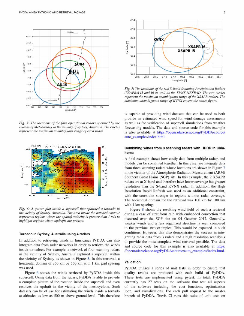
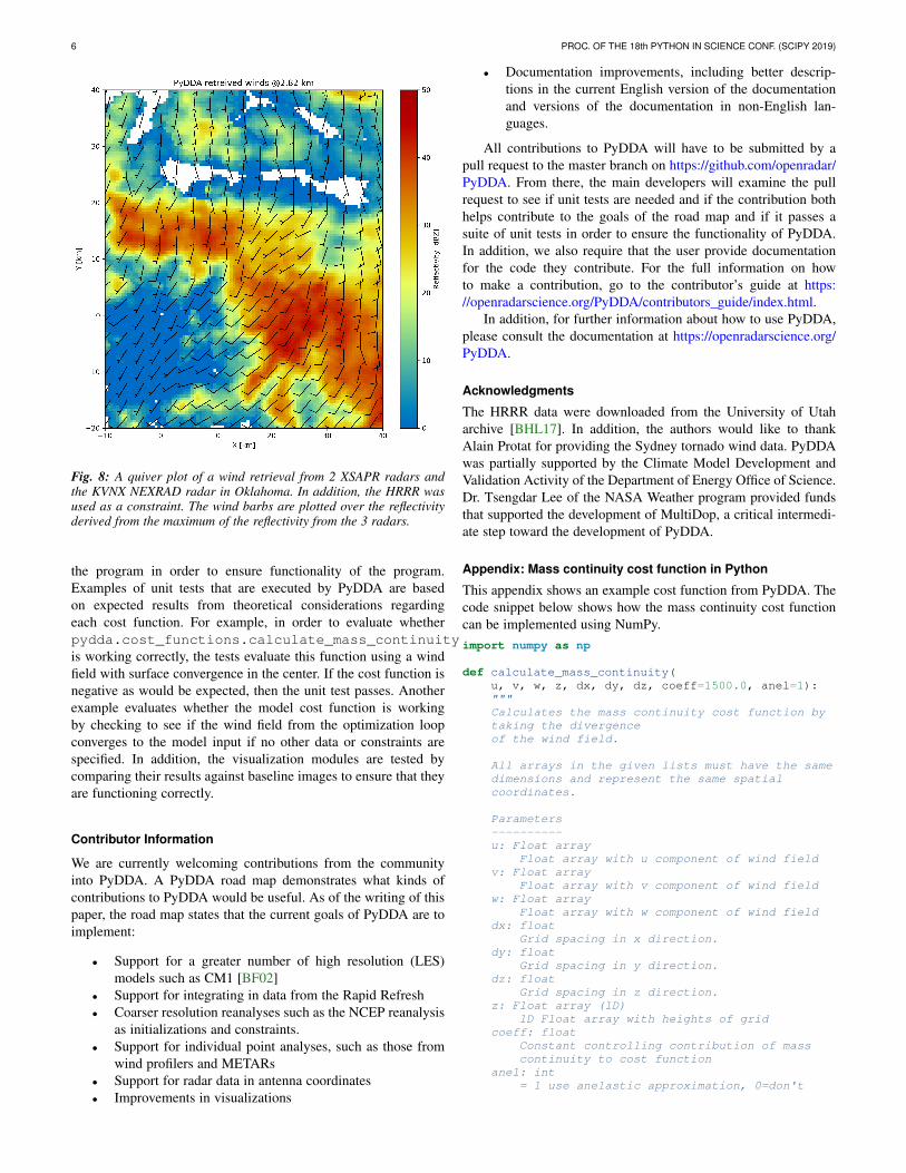
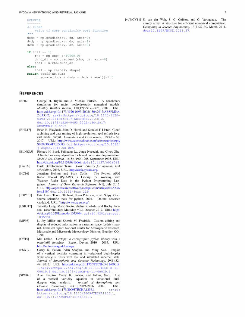