probabilistic methods applied to the
TRANSCRIPT


Probabilistic Methods applied to the
Bearing Capacity Problem
Von der Fakultät für Bau- und Umweltingenieurwissenschaften
der Universität Stuttgart
zur Erlangung der Würde eines Doktors der Ingenieurwissenschaften (Dr.-Ing.)
genehmigte Abhandlung,
vorgelegt von
CONSOLATA RUSSELLI
aus Turin (Italien)
Hauptberichter: Prof. Dr.-Ing. P.A. Vermeer
Mitberichter: Prof. Dr.-Ing. A. Bárdossy
Tag der mündlichen Prüfung: 14. Februar 2008
Institut für Geotechnik der Universität Stuttgart
2008
Mitteilung 58
des Instituts für Geotechnik
Universität Stuttgart, Germany, 2008
Editor:
Prof. Dr.-Ing. P. A. Vermeer
© Consolata Russelli
Institut für Geotechnik
Universität Stuttgart
Pfaffenwaldring 35
70569 Stuttgart
All rights reserved. No part of this publication may be reproduced, stored in a
retrieval system, or transmitted, in any form or by any means, electronic,
mechanical, photocopying, recording, scanning or otherwise, without the
permission in writing of the author.
Keywords: probabilistic methods, failure probability, bearing capacity
Printed by e.kurz + co, Stuttgart, Germany, 2008
ISBN 978-3-921837-58-0
(D93-Dissertation, Universität Stuttgart)

Preface
Traditional geotechnical analyses use a single “Factor of Safety”, which
implicitly includes all sources of variability and uncertainty inherent in the
geotechnical design. In foundation analysis for example, Terzaghi’s bearing
capacity equation leads to an estimate of the ultimate soil resistance, which is
then divided by a Factor of Safety to give allowable loading levels for design.
Meanwhile probabilistic geotechnical analyses have been proposed to include
the effects of soil property variability in a more scientific way. For the bearing
capacity problem, it implies that the soil properties such us the friction angle and
the cohesion are random variables that can be expressed in the form of
probability density functions. Meanwhile pioneering experimental studies have
been performed providing information on such functions for the random input
variables. Now the issue has become one of calculating the probability density
function of some outcome, such as the bearing capacity of a foundation. Mrs.
Consolata Russelli, focuses exactly on this problem.
On taking the bearing capacity of a footing as a benchmark problem, she
considers several stochastic procedures. Besides the well-known Monte-Carlo
simulations she uses approximations of first and second order. The main focus
of her study is the application of the Point Estimation Method (PEM), as
developed by Rosenblueth. She modifies this method by taking sampling points,
which suit the characteristics of the problem. On top of that she focuses on the
critical part of the curve. This is indeed a promising approach that merits further
research. No doubt, this so-called Advanced Point Estimation Method can also
be applied to slope stability and other geotechnical problems.
The financial support by the BMBF (Federal Ministry of Education and
Research) in the form of an IPSWAT1 scholarship to Mrs. Russelli is gratefully
acknowledged.
Prof. Dr.-Ing. P. A. Vermeer
Stuttgart, March 2008
1 IPSWAT stands for International Post-graduate Studies in Water Technologies


Acknowledgments
The research presented in this thesis is the result of the work carried out during
the years 2003-2007 at the Institute of Geotechnical Engineering (IGS) of
Stuttgart University. Behind this work there are important contributions and the
significant support of a certain number of persons, whom I would like to thank
sincerely.
First of all, I want to thank Prof. Dr.-Ing. Pieter A. Vermeer, Head of the
Institute of Geotechnical Engineering at Stuttgart University for providing me
with the opportunity to accomplish my doctoral studies under his excellent
supervision. No doubt, this doctoral research would not have been possible
without his support, patience and constant suggestions.
I would like to thank Prof. Dr. rer. Nat. Dr.-Ing. habil. András Bárdossy, Head
of the Department of Hydrology and Geohydrology of the Institute of Hydraulic
Engineering at Stuttgart University for his precious advice and constant
encouragement. His practical experience and technical knowledge made an
invaluable contribution to this thesis.
My sincere gratefulness to Prof. Dr.-Ing. Habil. Hermann Schad, Head of the
Geotechnical Department of the Otto-Graf-Institute, at the MPA Stuttgart and to
Ao. Univ.-Prof. Dipl.-Ing. Dr. techn. Helmut F. Schweiger, M.Sc., Head of the
Computational Geotechnics Group at the Institute for Soil Mechanics and
Foundation Engineering at Graz University of Technology for the interesting
discussions about important points of this thesis.
I would cordially thank the International Doctoral Program in the field of
“Environment Water” (ENWAT) of Stuttgart University and the German
Federal Ministry of Education and Research (Bundesministerium für Bildung
und Forschung, BMBF) for supporting my doctoral studies scientifically and
financially by granting me the IPSWaT (International Postgraduate Studies in
Water technology) scholarship for a duration of three years.
I would like to express my gratitude to all my colleagues of the Institute of
Geotechnical Engineering at Stuttgart University for their help, both
professional and moral, and for the very agreeable and stimulating working
atmosphere. I would especially thank my colleagues Dipl.-Ing. A. Möllmann
and Dr. Dipl.-Ing. M. Leoni and my friend C. Cimatoribus, Dr. candidate at the

Institute for Sanitary Engineering, Water Quality and Solid Waste Management
of Stuttgart University for the time spent with me for several discussions related
to my research and for their support in case of difficulties encountered during
my work.
Special thanks to Mr. G. Gay for correcting my English.
I also warmly thank my parents and my brother for supporting me throughout
my life. Even if hundred kilometers separate us, they have always been present
with their affection and love.
Finally I would like to thank Murat for being such a comprehensive and patient
husband. I will always remember his encouraging words during the hard times
of my doctoral studies.
Consolata Russelli
Stuttgart, April 2008

i
Contents
1 Introduction 1
1.1 Thesis purpose and motivation 1
1.2 Thesis restrictions 3
1.3 Thesis outline 4
2 Probabilistic concepts for geotechnical engineering 7
2.1 Uncertainty in Geotechnics 7
2.1.1 Sources of uncertainty 8
2.1.2 Types of uncertainty 9
2.2 Random variables 9
2.2.1 Main characteristics of random variables 10
2.2.1.1 The probability distribution and the probability density
functions 11
2.2.1.2 The mean value 12
2.2.1.3 The variance and the standard deviation 12
2.2.1.4 The coefficient of variation 13
2.2.1.5 The skewness 14
2.2.1.6 The covariance and the correlation coefficient 16
2.3 Useful continuous probability distributions of random variables 17
2.3.1 The normal and the standard normal distributions 18
2.3.2 The shifted and the standard lognormal distributions 19
2.4 The reliability analysis 21
2.4.1 The factor of safety 21
2.4.2 The safety margin and the failure probability 22
2.4.3 The reliability index 24
3 Probabilistic methods for quantifying uncertainties in Geotechnics 27
3.1 Monte Carlo Simulations (MCS) 27
3.2 The First Order Second Moment method (FOSM) 28
Contents
ii
3.2.1 Advantages and limitations of FOSM method 29
3.3 The Second Order Second Moment method (SOSM) 30
3.4 The Hasofer-Lind method (FORM) 31
3.4.1 Advantages and limitations of FORM method 32
3.5 The Two Point Estimate Method (PEM) 33
3.5.1 The procedure for implementing the PEM 34
3.5.2 Advantages and limitations of the PEM 37
4 Probabilistic analysis of the bearing capacity problem 41
4.1 Benchmarks on the bearing capacity of a strip footing 41
4.1.1 Benchmark 1: bearing capacity of a strip footing with effective
friction angle as input random variable 41
4.1.2 Benchmark 2: bearing capacity of a strip footing with effective
friction angle and cohesion as input random variables 42
4.2 Application of Monte Carlo Simulations 44
4.2.1 Monte Carlo results for benchmark 1 45
4.2.2 Monte Carlo results for benchmark 2 with uncorrelated soil
Parameters 47
4.2.3 Monte Carlo results for benchmark 2 with correlated soil parameters
50
4.3 Application of the FOSM method 55
4.3.1 FOSM results for benchmark 1 55
4.3.2 FOSM results for benchmark 2 with uncorrelated soil parameters 58
4.3.3 FOSM results for benchmark 2 with correlated soil parameters 60
4.4 Application of the SOSM method 62
4.4.1 SOSM results for benchmark 1 63
4.4.2 SOSM results for benchmark 2 with uncorrelated soil parameters 64
4.4.3 SOSM results for benchmark 2 with correlated soil parameters 66
4.5 Results comparison and necessity of an alternative method 68
4.5.1 Comparison of MCS, FOSM and SOSM results 68
4.5.2 Necessity of an alternative probabilistic method 72
5 The Two Point Estimate Method applied to the bearing capacity
problem 75
5.1 PEM results for benchmark 1 75
5.1.1 Procedure of the PEM 75
5.2 PEM results for benchmark 2 with uncorrelated soil parameters 78
5.2.1 Procedure of the PEM 78
Contents
iii
5.3 PEM results for benchmark 2 with correlated soil parameters 81
5.3.1 Procedure of the PEM 82
5.4 Comparison of PEM, MCS, FOSM and SOSM results 88
5.4.1 Comparison of results for benchmark 1 88
5.4.2 Comparison of results for benchmark 2 with uncorrelated soil
parameters 91
5.4.3 Comparison of results for benchmark 2 with correlated soil
parameters 93
5.5 Discussion of the assumption of the shifted lognormal distribution 94
5.6 Conclusions on the application of the PEM to the bearing capacity
problem 102
6 The Advanced Point Estimate Method (APEM) for the reliability
analysis 103
6.1 Basic problems concerning the evaluation of failure probabilities 103
6.2 Reliability analysis of the bearing capacity problem 104
6.2.1 Failure probability from Monte Carlo simulations 105
6.2.2 Failure probability from FOSM and SOSM methods 110
6.2.3 Failure probability from FORM 112
6.2.4 Failure probability from PEM 113
6.2.5 Comparison of failure probabilities and necessity of a new approach
115
6.3 Application of the Advanced PEM to the bearing capacity problem 121
6.3.1 Short description of the Advanced PEM methodology 121
6.3.2 The reduced intervals of the input soil parameters 121
6.3.3 Application of the PEM to the reduced intervals of the soil
parameters 123
6.3.3.1 Case with ρc´tanϕ´ = 0 123
6.3.3.2 Case with ρc´tanϕ´ = -0.6 126
6.3.4 Shifted lognormal approximation of the bearing capacity results 127
6.3.4.1 Procedure to find the shifted lognormal parameters 128
6.4 Results comparison of MCS, traditional PEM and APEM 130
6.4.1 Case with ρc´tanϕ´ = 0 130
6.4.2 Case with ρc´tanϕ´ = -0.6 133
6.5 Applicability of the estimated failure probability of the bearing capacity
136
Contents
iv
7 Conclusions and recommendations for further research 139
7.1 General conclusions 139
7.2 Conclusions with respect to the probabilistic methods applied to the
bearing capacity problem 140
7.3 Conclusions with respect to the Two Point Estimate Method 141
7.4 Conclusions with respect to the shifted lognormal distribution 142
7.5 Conclusions with respect to the correlation between the soil parameters c´
and tanϕ´ 143
7.6 Conclusions with respect to the reliability analysis 144
7.7 Conclusions with respect to the APEM 145
7.8 Recommendations for further research 146
Appendix 149
A The Terzaghi’s bearing capacity formula 149
B Derivatives of the bearing capacity for the FOSM and SOSM methods 152
C Algorithm to evaluate the reduced intervals of the input soil parameters
154
D Algorithm to evaluate the shifted lognormal parameters and the failure
probability of the bearing capacity problem 156
D.1 Main routine for the estimation of the three shifted lognormal
parameters 156
D.2 Subroutine for the evaluation of the integrals of the objective function
158
D.3 Subroutines for the definition of the integrals of the objective function
161
D.4 Optimisation results for the bearing capacity problem 162
D.4.1 Case with ρc´tanϕ´ = 0 162
D.4.2 Case with ρc´tanϕ´ = -0.6 163
Bibliography 165
v
Abstract
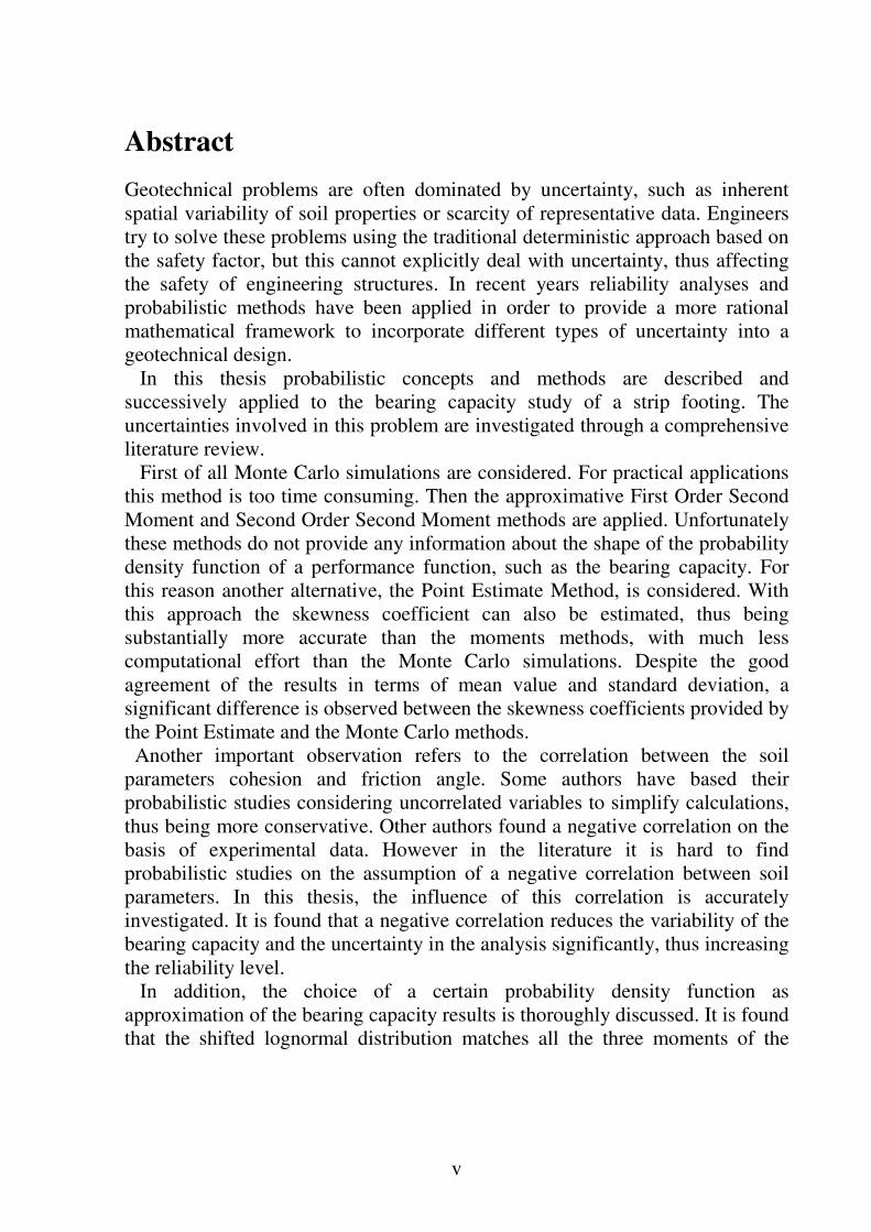
Geotechnical problems are often dominated by uncertainty, such as inherent
spatial variability of soil properties or scarcity of representative data. Engineers
try to solve these problems using the traditional deterministic approach based on
the safety factor, but this cannot explicitly deal with uncertainty, thus affecting
the safety of engineering structures. In recent years reliability analyses and
probabilistic methods have been applied in order to provide a more rational
mathematical framework to incorporate different types of uncertainty into a
geotechnical design.
In this thesis probabilistic concepts and methods are described and
successively applied to the bearing capacity study of a strip footing. The
uncertainties involved in this problem are investigated through a comprehensive
literature review.
First of all Monte Carlo simulations are considered. For practical applications
this method is too time consuming. Then the approximative First Order Second
Moment and Second Order Second Moment methods are applied. Unfortunately
these methods do not provide any information about the shape of the probability
density function of a performance function, such as the bearing capacity. For
this reason another alternative, the Point Estimate Method, is considered. With
this approach the skewness coefficient can also be estimated, thus being
substantially more accurate than the moments methods, with much less
computational effort than the Monte Carlo simulations. Despite the good
agreement of the results in terms of mean value and standard deviation, a
significant difference is observed between the skewness coefficients provided by
the Point Estimate and the Monte Carlo methods.
Another important observation refers to the correlation between the soil
parameters cohesion and friction angle. Some authors have based their
probabilistic studies considering uncorrelated variables to simplify calculations,
thus being more conservative. Other authors found a negative correlation on the
basis of experimental data. However in the literature it is hard to find
probabilistic studies on the assumption of a negative correlation between soil
parameters. In this thesis, the influence of this correlation is accurately
investigated. It is found that a negative correlation reduces the variability of the
bearing capacity and the uncertainty in the analysis significantly, thus increasing
the reliability level.
In addition, the choice of a certain probability density function as
approximation of the bearing capacity results is thoroughly discussed. It is found
that the shifted lognormal distribution matches all the three moments of the

Abstract
vi
bearing capacity extremely well, i.e. mean value, standard deviation and
skewness, thus being more accurate than other distributions.
The reliability analysis of the bearing capacity problem shows that the results
of the Point Estimate method approximated by the shifted lognormal distribution
do not match the low failure probabilities evaluated using MCS very well. In
order to cope with the shortcoming of the Point Estimate method in assessing
small values of the failure probability, a new method is developed, referred to as
the advanced Point Estimate method. The proposed method is also applied to the
bearing capacity problem and the results are then validated using the Monte
Carlo approach.
vii
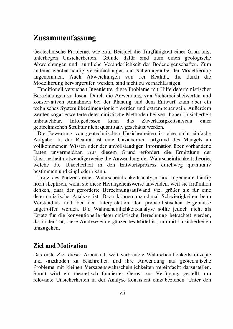
Zusammenfassung
Geotechnische Probleme, wie zum Beispiel die Tragfähigkeit einer Gründung,
unterliegen Unsicherheiten. Gründe dafür sind zum einen geologische
Abweichungen und räumliche Veränderlichkeit der Bodeneigenschaften. Zum
anderen werden häufig Vereinfachungen und Näherungen bei der Modellierung
angenommen. Auch Abweichungen von der Realität, die durch die
Modellierung hervorgerufen werden, sind nicht zu vernachlässigen.
Traditionell versuchen Ingenieure, diese Probleme mit Hilfe deterministischer
Berechnungen zu lösen. Durch die Anwendung von Sicherheitsbeiwerten und
konservativen Annahmen bei der Planung und dem Entwurf kann aber ein
technisches System überdimensioniert werden und extrem teuer sein. Außerdem
werden sogar erweiterte deterministische Methoden bei sehr hoher Unsicherheit
unbrauchbar. Infolgedessen kann das Zuverlässigkeitsniveau einer
geotechnischen Struktur nicht quantitativ geschätzt werden.
Die Bewertung von geotechnischen Unsicherheiten ist eine nicht einfache
Aufgabe. In der Realität ist eine Unsicherheit aufgrund des Mangels an
vollkommenem Wissen oder der unvollständigen Information über vorhandene
Daten unvermeidbar. Aus diesem Grund erfordert die Ermittlung der
Unsicherheit notwendigerweise die Anwendung der Wahrscheinlichkeitstheorie,
welche die Unsicherheit in den Entwurfsprozess durchweg quantitativ
bestimmen und eingliedern kann.
Trotz des Nutzens einer Wahrscheinlichkeitsanalyse sind Ingenieure häufig
noch skeptisch, wenn sie diese Herangehensweise anwenden, weil sie irrtümlich
denken, dass der geforderte Berechnungsaufwand viel größer als für eine
deterministische Analyse ist. Dazu können manchmal Schwierigkeiten beim
Verständnis und bei der Interpretation der probabilistischen Ergebnisse
angetroffen werden. Die Wahrscheinlichkeitsanalyse sollte jedoch nicht als
Ersatz für die konventionelle deterministische Berechnung betrachtet werden,
da, in der Tat, diese Analyse ein ergänzendes Mittel ist, um mit Unsicherheiten
umzugehen.
Ziel und Motivation
Das erste Ziel dieser Arbeit ist, weit verbreitete Wahrscheinlichkeitskonzepte
und -methoden zu beschreiben und ihre Anwendung auf geotechnische
Probleme mit kleinen Versagenswahrscheinlichkeiten vereinfacht darzustellen.
Somit wird ein theoretisch fundiertes Gerüst zur Verfügung gestellt, um
relevante Unsicherheiten in der Analyse konsistent einzubeziehen. Unter den

Zusammenfassung
viii
vorhandenen Wahrscheinlichkeitsmethoden werden dann Verfahren für eine
weitere Analyse gewählt, die für geotechnische Probleme am besten geeignet
sind.
Außerdem wird in vorliegender Arbeit eine neue Wahrscheinlichkeitsmethode
entwickelt, welche die Einschränkungen anderer Methoden überwinden kann,
besonders für die Auswertung der kleinen Versagenswahrscheinlichkeiten einer
geotechnischen Struktur. Um von praktischen Ingenieuren angenommen zu
werden, sollte diese neue Methode für Zuverlässigkeit- und Risikoanalysen
geotechnischer Probleme leicht anwendbar sein und sowohl Expertenwissen als
auch Entscheidungsträger unterstützen.
Zu diesem Zweck wird ein einfaches Beispielproblem betrachtet, die Analyse
der Grundbruchtragfähigkeit einer Flachgründung auf einer homogenen
Bodenschicht, für die eine analytische Lösung zur Verfügung steht. Aufgrund
der natürlichen Streuung der Scherfestigkeitsparameter werden die effektive
Bodenkohäsion und der effektive Reibungswinkel als Zufallsvariablen
angenommen und durch bekannte Verteilungsfunktionen beschrieben. Andere
Bodenparameter, die nicht abhängig von irgendeiner bedeutenden Streuung sind,
werden deterministisch behandelt, um die Komplexität des Problems zu
verringern.
Zuerst kommen Monte-Carlo Simulationen (MCS) zur Anwendung. Um
genaue statistische Werte zu erhalten, werden mindestens zehntausend
Realisierungen innerhalb des betrachteten Bereiches der Bodenparameter
ausgewertet. Da diese Methode in der Praxis allzu rechenintensiv und
zeitaufwändig ist, werden andere Methoden wie die Momentenmethoden FOSM
(First Order Second Moment) und SOSM (Second Order Second Moment)
angewendet, bei denen um den Mittelwert der Eingangsparameter linearisiert
wird. Eine andere Näherungsverfahren ist das Punktabschätzverfahren (PEM)
nach ROSENBLUETH (1975, 1981). Bei der PEM wird die Verteilungsfunktion
der Scherfestigkeitsparameter diskretisiert, indem man einige Stützpunkte wählt.
Danach können der Mittelwert, die Standardabweichung und die Schiefe der
Grundbruchtragfähigkeit durch gewichtetes Aufsummieren der diskreten
Realisationen (Stützpunkte) ermittelt werden. Die PEM benötigt mehr
Berechnungsaufwand als die Methoden FOSM und SOSM. Die Ergebnisse sind
jedoch wesentlich genauer, weil diese Annäherung nicht nur Mittelwert und
Standardabweichung der Grundbruchtragfähigkeit auswertet, sondern auch
deren Schiefekoeffizient.
In dieser Arbeit werden auch die Ergebnisse der Zuverlässigkeitsanalyse des
Grundbruchtragfähigkeitsproblems gezeigt, indem die bereits erwähnten
Wahrscheinlichkeitsverfahren angewendet werden.
Zusammenfassung
ix
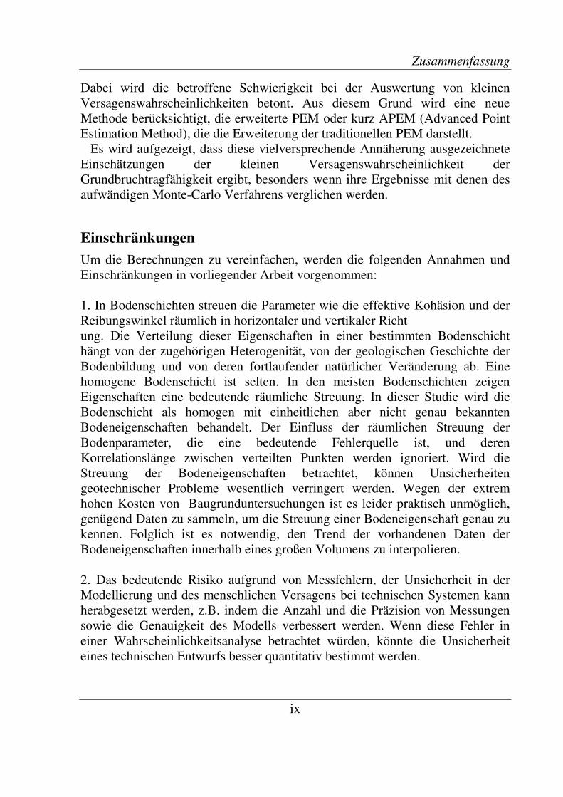
Dabei wird die betroffene Schwierigkeit bei der Auswertung von kleinen
Versagenswahrscheinlichkeiten betont. Aus diesem Grund wird eine neue
Methode berücksichtigt, die erweiterte PEM oder kurz APEM (Advanced Point
Estimation Method), die die Erweiterung der traditionellen PEM darstellt.
Es wird aufgezeigt, dass diese vielversprechende Annäherung ausgezeichnete
Einschätzungen der kleinen Versagenswahrscheinlichkeit der
Grundbruchtragfähigkeit ergibt, besonders wenn ihre Ergebnisse mit denen des
aufwändigen Monte-Carlo Verfahrens verglichen werden.
Einschränkungen
Um die Berechnungen zu vereinfachen, werden die folgenden Annahmen und
Einschränkungen in vorliegender Arbeit vorgenommen:
1. In Bodenschichten streuen die Parameter wie die effektive Kohäsion und der
Reibungswinkel räumlich in horizontaler und vertikaler Richt
ung. Die Verteilung dieser Eigenschaften in einer bestimmten Bodenschicht
hängt von der zugehörigen Heterogenität, von der geologischen Geschichte der
Bodenbildung und von deren fortlaufender natürlicher Veränderung ab. Eine
homogene Bodenschicht ist selten. In den meisten Bodenschichten zeigen
Eigenschaften eine bedeutende räumliche Streuung. In dieser Studie wird die
Bodenschicht als homogen mit einheitlichen aber nicht genau bekannten
Bodeneigenschaften behandelt. Der Einfluss der räumlichen Streuung der
Bodenparameter, die eine bedeutende Fehlerquelle ist, und deren
Korrelationslänge zwischen verteilten Punkten werden ignoriert. Wird die
Streuung der Bodeneigenschaften betrachtet, können Unsicherheiten
geotechnischer Probleme wesentlich verringert werden. Wegen der extrem
hohen Kosten von Baugrunduntersuchungen ist es leider praktisch unmöglich,
genügend Daten zu sammeln, um die Streuung einer Bodeneigenschaft genau zu
kennen. Folglich ist es notwendig, den Trend der vorhandenen Daten der
Bodeneigenschaften innerhalb eines großen Volumens zu interpolieren.
2. Das bedeutende Risiko aufgrund von Messfehlern, der Unsicherheit in der
Modellierung und des menschlichen Versagens bei technischen Systemen kann
herabgesetzt werden, z.B. indem die Anzahl und die Präzision von Messungen
sowie die Genauigkeit des Modells verbessert werden. Wenn diese Fehler in
einer Wahrscheinlichkeitsanalyse betrachtet würden, könnte die Unsicherheit
eines technischen Entwurfs besser quantitativ bestimmt werden.
Zusammenfassung
x
3. Trotz der Bemühungen, Unsicherheiten der Bodeneigenschaften in einer
Wahrscheinlichkeitsanalyse zu berücksichtigen, besteht immer die Möglichkeit,
einige von ihnen zu vernachlässigen. Dieses könnte die Lösung eines
bestimmten geotechnischen Problems erheblich beeinflussen. Zusätzlich werden
häufig viele Parameter nicht behandelt, um Wahrscheinlichkeitsanalysen zu
vereinfachen. Auf diese Weise wird ihr Beitrag nicht betrachtet, wenn man das
Zuverlässigkeitsniveau eines technischen Systems auswertet. Deshalb kann die
berechnete Versagenswahrscheinlichkeit nur als unterere Grenze zur absoluten
Versagenswahrscheinlichkeit angesehen werden. Eine anspruchsvollere
Risikoanalyse wäre erforderlich, um das Risiko weiterer nicht berücksichtigter
Unsicherheiten miteinzubeziehen.
Überblick
In diesem Zusammenhang werden die folgenden Kapitel berücksichtigt:
Kapitel 2: Dieses Kapitel beginnt mit der Berücksichtigung von wesentlichen
Quellen und Arten der Unsicherheit im Bereich der Geotechnik. Die wichtige
Rolle der Anwendung von Wahrscheinlichkeitsmethoden als Alternative zur
deterministischen Analyse wird betont, um Unsicherheiten quantitativ zu
bestimmen. Es folgt nachher eine Beschreibung der wichtigsten Statistik- und
Wahrscheinlichkeitskonzepte von Zufallsvariablen, welche für diese Arbeit
relevant sind. Eine Definition von Zufallsvariablen wird dann gegeben. Dabei
werden ihre Haupteigenschaften und einige nützliche Verteilungsfunktionen
beschrieben. Schließlich hebt das Kapitel die Bedeutung des Durchführens einer
Zuverlässigkeitsanalyse und des Auswertens der Versagenswahrscheinlichkeit
eines technischen Entwurfs hervor. Es wird gezeigt, wie sich der traditionelle
Sicherheitsbeiwert zu der Versagenswahrscheinlichkeit, welche ein
realistischeres Maß eines Zuverlässigkeitssystems ist, in Beziehung setzt.
Kapitel 3: Ziel dieses Kapitels ist, einige weithin bekannte
Wahrscheinlichkeitsmethoden zu erläutern, mit denen vorhandene
Unsicherheiten rationeller behandelt und Wahrscheinlichkeitskonzepte in
geotechnische Analysen einbezogen werden können. Besondere
Aufmerksamkeit wird den Monte-Carlo Simulationen (MCS), dem
Punktabschätzverfahren (PEM), den Momentenmethoden FORM, FOSM und
SOSM gewidmet. Die Vorgehensweise dieser Methoden wird weitgehend
veranschaulicht und die entsprechenden Vorteile und Einschränkungen
diskutiert.
Zusammenfassung
xi
Kapitel 4: Dieses Kapitel behandelt eine mögliche Anwendung der Methoden
MCS, FOSM und SOSM zur Grundbruchtragfähigkeit eines Streifenfundaments
auf einer homogenen Bodenschicht. Zwei Fallstudien werden vorgestellt, für
welche die effektive Kohäsion und der effektive Reibungswinkel als
Zufallsvariablen angenommen werden, da diese die größte Auswirkung auf die
Baugrundtragfähigkeit haben. Unterschiedliche Werte des
Korrelationskoeffizienten zwischen den Bodenparametern werden betrachtet.
Insbesondere wenn die Ergebnisse der oben genannten Methoden verglichen
werden, wird aufgezeigt, wie die Korrelation die Wahrscheinlichkeitsanalyse
stark beeinflusst, da die Streuung der Grundbruchtragfähigkeit und die
Unsicherheit erheblich verringert werden. Schließlich wird der Bedarf einer
alternativen Methode angesprochen, welche die Einschränkungen der Methoden
MCS, FOSM und SOSM bewältigen kann.
Kapitel 5: In diesem Kapitel wird gezeigt, wie die PEM die Einschränkungen
der Methoden MCS, FOSM und SOSM überwinden kann. Daher erweist sich
die PEM als eine attraktive und leistungsfähige Alternative zu den anderen
Wahrscheinlichkeitsmethoden, da sie weniger Berechnungsaufwand erfordert.
Aus diesem Grund wird die PEM auf das Grundbruchtragfähigkeitsproblem
angewendet. Ihre Ergebnisse werden dann mit denen der Verfahren MCS,
FOSM und SOSM verglichen. Es wird gezeigt, dass die Ergebnisse der PEM
genauer als die der Methoden FOSM und SOSM sind; jedoch wird ein
bedeutender Unterschied zwischen den Schiefekoeffizienten von PEM und MCS
beobachtet. Zusätzlich werden die Bedeutung und der Einfluss der Korrelation
zwischen Bodenparametern bei der Anwendung der PEM hervorgehoben.
Kapitel 6: Dieses Kapitel greift die grundlegenden Probleme der
Zuverlässigkeitsanalyse auf, die auf der Auswertung einer kleinen
Versagenswahrscheinlichkeit fokussiert. Zunächst werden die Ergebnisse der
Zuverlässigkeitsanalyse des Grundbruchtragfähigkeitsproblems, welche in
Versagenswahrscheinlichkeit und Zuverlässigkeitsindex ausgedrückt werden,
dargestellt und verglichen, indem bekannte Wahrscheinlichkeitsmethoden
einschließlich MCS und PEM verwendet werden. Um die Einschränkungen der
PEM bei der Ermittlung einer kleinen Versagenswahrscheinlichkeit zu
überwinden, wird danach eine sogenannte erweiterte PEM (kurz APEM)
eingeführt. Diese ist in der Literatur bislang nicht behandelt worden. Die
Grundidee dieser Methode ist, Augenmerk auf die verhältnismäßig kleinen
Werte der Bodenkohäsion und des Reibungswinkels zu richten, die zum
Versagen führen.

Zusammenfassung
xii
Die APEM wird auf verringerte Intervalle der Scherfestigkeitsparameter
angewendet, um die Versagenswahrscheinlichkeit der Grundbruchtragfähigkeit
genauer abzuschätzen. Dieser Wert wird dann mit der ermittelten
Versagenswahrscheinlichkeit der MCS verglichen, um die Genauigkeit der
APEM zu bestimmen.
Kapitel 7: Die relevantesten Ergebnisse dieser Arbeit werden im
abschließenden Kapitel zusammengefasst. Darüber hinaus werden die
wichtigsten Schlussfolgerungen aufgegriffen und Empfehlungen für
weiterführende Forschungsprojekte gegeben.
1
Chapter 1
Introduction It has long been recognised that uncertainties, such as the inherent spatial
variability of soil properties, often dominate many events or problems of interest
to geotechnical engineers. Traditionally engineers try to solve these problems by
deterministic calculation through the use of safety factors and adopting
conservative assumptions in the process of engineering planning and design. In
this way an engineering system can be over-designed and extremely expensive.
Furthermore, even advanced deterministic methods become useless when the
uncertainty is very high. As a result the reliability level of a geotechnical
structure cannot be estimated quantitatively.
The assessment of geotechnical uncertainties is not an easy task. As a matter
of fact uncertainty is unavoidable, due to the lack of perfect knowledge or to the
incomplete information about available data. For this reason the determination
of uncertainty necessarily requires the application of probability theory, which
quantifies and integrates uncertainty into the design process in a consistent
manner.
Despite the benefits gained from a probabilistic analysis, engineers are often
still sceptical in adopting this approach, because they think, erroneously, that the
calculation effort required is much larger than for a deterministic analysis. In
addition, difficulties are sometimes encountered in understanding and
interpreting probabilistic results.
Probabilistic analysis should not however be considered as a substitute for the
conventional deterministic design, it is in fact a complementary measure to deal
with uncertainties.
1.1 Thesis purpose and motivation
The first object of this research is to describe well-known probabilistic concepts
and methods and show their application to geotechnical low probability
estimation problems in a straightforward way, thus providing a rational
framework to incorporate consistently relevant uncertainties in the analysis.
Chapter 1 Introduction
2
Among the available probabilistic approaches, the ones most suitable for the
geotechnical field will be then chosen for a further analysis.
Moreover, in the present thesis a new probabilistic approach will be
developed, which should be able to cope with the shortcomings of other
methods, especially for the evaluation of low failure probabilities of a
geotechnical structure. In order to be accepted by practical engineers, this new
method should be easily applicable for reliability and risk analyses of
geotechnical problems, supporting both engineering judgement and decision
making.
To achieve these aims a simple example problem is analysed: the bearing
capacity study of a strip footing on a homogeneous soil layer, for which an
analytical solution is available. The soil shear strength parameters, i.e. the
effective cohesion and friction angle, are described by specific probabilistic
distribution functions. While other soil parameters that are not subject to any
significant variation are treated deterministically to reduce the complexity of the
problem.
Initially Monte Carlo simulations (MCS) are applied. In order to obtain
accurate statistical values at least ten thousand realisations are required within
the considered range of soil parameters. Since this method is too complex and
time consuming for the practice, other methods are examined, such as the First
Order Second Moment (FOSM) and the Second Order Second Moment (SOSM)
methods, which produce a linearization around the average values of the input
random variables. Another approximation method is the Point Estimate Method
(PEM) after ROSENBLUETH (1975, 1981). With the PEM a continuous
distribution curve is replaced by particularly specified discrete probabilities and
the first three moments of a probability distribution function, i.e. mean value,
standard deviation and skewness, can be defined. The determination of these
moments is realized through the weighted sum of every discrete realizations,
also referred to as sampling points. The PEM requires more computational effort
than FOSM and SOSM methods. The results however are substantially more
accurate, because this approach evaluates not only mean value and standard
deviation of the bearing capacity, but also its skewness coefficient.
In this thesis, the results of the reliability analysis of the bearing capacity
problem by applying the already mentioned probabilistic techniques will also be
shown, stressing the difficulty encountered in evaluating low failure
probabilities. For this reason a new approach is taking into account, the
advanced PEM, or shortly APEM, which represents the enhancement of the
traditional Point Estimate method.
1.2 Thesis restrictions
3
This promising technique will be shown to give excellent predictions of the
failure behaviour of the bearing capacity, especially when its results will be
compared with those of Monte Carlo method.
1.2 Thesis restrictions
In order to simplify the calculations, the following assumptions and restrictions
are adopted in this research:
1. In soil layers parameters, such as the effective cohesion and the friction angle,
vary spatially in both horizontal and vertical directions. The distribution of these
properties on a particular soil layer depends on the inherent heterogeneity, the
geological history of soil formation and its continuous modification by nature. A
homogeneous soil layer is rare. In most soil layers properties show a significant
variation over space.
This study is carried out by treating the soil layer as homogeneous with
uniform, but not exactly known, soil properties. The influence of the spatial
variability of soil parameters, which is a significant source of error, and the
correlation length (or scale of fluctuation) between the different points of the
random field are ignored. Taking into account the variability in soil properties
when predicting geotechnical performance may substantially reduce the
uncertainties associated with a design. Unfortunately, because of the extremely
high costs of subsurface investigations, it is practically impossible to collect
enough data to exactly understand the variation of a soil property. Therefore it is
necessary to interpolate the trend of the available data of soil properties within a
large volume.
2. The significant risk due to the measurement, model and human errors in
engineering systems can be minimized, for example, by improving the quantity
and precision of measurements, the accuracy of the model and the quality
assurance and control system. When these errors are taken into account in a
probabilistic analysis, the uncertainty of an engineering design could be better
quantified.
3. Notwithstanding the efforts of including soil properties uncertainties in a
probabilistic analysis, there is always the possibility of missing some of them.
This could affect the solution of a certain geotechnical problem significantly.
Additionally many parameters are not usually taken into account in order to
simplify probabilistic analyses. In this way their contribution is not considered

Chapter 1 Introduction
4
in evaluating the reliability level of an engineering system and the computed
failure probability can only be seen as a lower bound to the absolute failure
probability. A more sophisticated probabilistic risk analysis would be needed to
assess the risk due to all undetected events.
1.3 Thesis outline
In order to achieve the objects of the present research discussed in section 1.1,
the following chapters will be considered:
Chapter 2: this chapter starts by considering the primary sources and types of
uncertainty in the geotechnical field, underlying the importance of using
probabilistic methods as alternative to the deterministic analysis to quantify
uncertainties. Hereafter follows a description of the most important statistical
and probabilistic concepts of continuous random variables, which are relevant to
this research. A definition of random variables is then provided by describing its
main characteristics and some useful continuous probability distributions.
Finally the chapter will highlight the importance of carrying out a reliability
analysis and of evaluating the failure probability of an engineering design. It is
shown how the traditional safety factor relates to the probability of failure, the
latter representing a more realistic measure of a system reliability.
Chapter 3: the aim of this chapter is to review some well-known probabilistic
techniques for dealing with uncertainties and for implementing probabilistic
concepts into geotechnical analyses in a more rational way. Particular attention
is given to Monte Carlo Simulations (MCS), the Point Estimate method (PEM),
the First Order Reliability (FORM) method, the First Order Second Moment
(FOSM) and the Second Order Second Moment (SOSM) methods. The
methodologies are extensively illustrated and the corresponding advantages and
limitations are discussed.
Chapter 4: this chapter presents a possible application of the probabilistic
methods MCS, FOSM and SOSM to the bearing capacity study of a strip footing
on a homogeneous soil layer characterised by the corresponding effective
cohesion and friction angle. Two benchmarks are introduced, for which the
effective cohesion and friction angle are considered as random variables, since
they have the greatest impact on the soil bearing capacity. Different values of
the correlation coefficient between the soil parameters will be taken into
account. In particular, when the final results of MCS, FOSM and SOSM
1.3 Thesis outline
5
methods are compared, it will be shown how this correlation strongly influences
the probabilistic analysis, reducing the variability of the bearing capacity and the
uncertainty in the final results significantly. Finally, the necessity of an
alternative probabilistic approach, which could cope with the shortcomings of
MCS, FOSM and SOSM methods, will be discussed.
Chapter 5: the purpose of this chapter is to show how the PEM can overcome
the drawbacks of MCS, FOSM and SOSM methods, thus resulting to be an
attractive alternative to the other probabilistic methods in terms of
computational effort and mathematical simplicity. For this reason, the PEM is
also applied to the bearing capacity benchmarks described in chapter 4 and the
results are then compared with those of MCS, FOSM and SOSM methods. It
will be shown that the PEM results are more accurate than FOSM and SOSM
methods; however a large difference between the skewness coefficients of PEM
and MCS will be seen. In addition, it will be stressed that care should be taken in
applying the PEM when a correlation between soil parameters is considered.
Chapter 6: this chapter starts with a discussion of the basic problems
concerning the reliability analysis of engineering systems, focusing on the
evaluation of small values of the failure probability. Next, the results of the
reliability analysis of the bearing capacity problem by applying well-known
probabilistic approaches, including MCS and PEM, are presented and compared,
both in terms of failure probability and reliability index. Afterwards, in order to
cope with the shortcomings of the PEM for the assessment of small values of the
failure probability, a so called advanced PEM, or shortly APEM, is introduced.
This has not been previously mentioned in the literature. The basic idea of this
method is to focus on the relatively small values of soil cohesion and friction
angle, which would most probably cause bearing capacity failure. The APEM
will be applied to the reduced intervals of the soil strength parameters to predict
the failure behaviour of the bearing capacity. Finally, the applicability of the
estimated failure probabilities of the bearing capacity is discussed using
diagrams usually employed in decision-making.
Chapter 7: a summary of the most relevant findings of this research is
presented in the final chapter, drawing conclusions and including
recommendations for further research.


7
Chapter 2
Probabilistic concepts for geotechnical
engineering
Introduction The purpose of this chapter is to provide the most important statistical and
probabilistic concepts of continuous random variables, which are fundamental
for this study, such as the mean value or the standard deviation. For more
detailed descriptions about the mathematical background of probability theory
the author refers to ANG and TANG (1975).
The chapter begins by considering the primary sources and types of
uncertainty in the geotechnical field, underlying the importance of using
probabilistic methods as an alternative to the deterministic analysis to quantify
uncertainties.
It continues by providing a definition of random variables and by describing
their main characteristics and some useful continuous probability distributions.
Finally the chapter will address the reliability analysis, highlighting the
importance of evaluating the failure probability of an engineering system.
2.1 Uncertainty in Geotechnics
Many sources of uncertainty exist in the geotechnical field ranging from the
variability of soil properties to the sampling and testing technique. Engineers try
to cope with these problems using deterministic analyses, which are based on
the classical notion of the safety factor.
However practical experience shows that the deterministic approach, relying
on conservative designs, which are not always safe against failure, is not suitable
for dealing rationally with uncertainty. As a result, the reliability of a system can
not be properly assessed. This fact will be better explained in section 2.4.
The authors EINSTEIN and BÄCHER (1982) stated in one of their papers that:

Chapter 2 Probabilistic concepts for geotechnical engineering
8
ESTIMATED
SOIL PROPERTY
SOIL
LAYER
inherent
soil layer
variability
IN-SITU
MEASUREMENT
data
scatter
statistical
uncertainty
inherent
soil
variability
measurement
error
TRANSFORMATION
MODEL
model
uncertainty
natural
geologic
processes
degree of equipment
and procedural control,
random testing effects,
sampling error
field and laboratory
measurements
transformed into design
soil properties using
empirical or other
correlation models
REAL WORLD IDEALISATION
„In thinking about sources of uncertainty in engineering geology, one is left
with the fact that uncertainty is inevitable. One attempts to reduce it as much as
possible, but it must ultimately be faced. […]. The question is not whether to
deal with uncertainty, but how?”.
In this regard, a rigorous evaluation of the uncertainty involved in geotechnical
problems necessarily requires the application of probabilistic theory as a
complement to conventional deterministic analyses. In fact probabilistic
concepts and methods, associated to the statistical theory, offer a theoretical
basis for quantifying uncertainties consistently, rendering them into precise
mathematical terms. In this way, a logical framework is provided for reliability
and risk analysis.
2.1.1 Sources of uncertainty
Geotechnical variability results from different sources of uncertainties. The three
primary sources are inherent variability, measurement error and model
uncertainty, as described in Fig. 2.1.
Figure 2.1: Uncertainty in soil property estimates (KULHAWY, 1992)

2.2 Random variables
9
Inherent variability results primarily from natural geologic processes that
created in-situ soil layers. Measurement error is caused by sampling and
laboratory testing.
This error is increased by statistical uncertainty that arises from limited
amount of information. Finally the model uncertainty is introduced when field or
laboratory measurements are transformed into input parameters for design
models involving simplifications and idealisations.
2.1.2 Types of uncertainty
Uncertainties associated with geotechnical engineering can be divided into three
categories: the inherent or natural uncertainty (aleatory), the uncertainties due to
the lack of perfect knowledge (epistemic) and the human error.
The aleatory (from Latin aleator meaning “gambler” or alea meaning “die”)
uncertainty is attributed to the natural variability or randomness of a certain
property, such as the spatial variation of the soil layer properties cohesion and
friction angle. It could be quantified by measurements and statistical estimations
or by expert opinion. This kind of uncertainty is unpredictable and therefore
irreducible via collection of more experimental data or use of more refined
models. For this type of uncertainty the term probability means the frequency of
occurrence of a random event, which is an innate property of nature.
The epistemic (from Greek επιστηµη meaning “knowledge”) uncertainty
arises from the lack of knowledge of a system and it is related to limited or
ambiguous data, measurement error, incomplete knowledge, imperfect models
and subjective judgement. It can in principle be quantified by experts, but not
measured. This kind of uncertainty can be reduced by collecting more
experimental data, by improving the measurement and calculation methods and
by using more refined models. For this type of uncertainty the term probability
means the degree of belief in the occurrence of a random event, which is a
subjective interpretation of the individual, e.g. the engineering judgement of an
expert.
In Geotechnics aleatory and epistemic uncertainties coexist in most practical
applications.
2.2 Random variables
In a probabilistic analysis the geotechnical parameters, which represent the
major sources of uncertainties, are treated as random variables.
A random variable is a mathematical function defined on a sample space that
assigns a probability to each possible event within the sample space.

Chapter 2 Probabilistic concepts for geotechnical engineering
10
Fre
quency o
f occu
rrence
, %
Event X
0 10 20 30 40 50 60
0.1
0.2
0.3
0.4
0.5
0.6
0.7
0
Fre
quency o
f occu
rrence
, %
Event X
0 10 20 30 40 50
0.1
0.2
0.3
0.4
0.5
0.6
0.7
0
Fre
quency o
f occu
rrence
, %
Event X
0 10 20 30 40 50 60
0.1
0.2
0.3
0.4
0.5
0.6
0.7
0
Fre
quency o
f occu
rrence
, %
Event X
0 10 20 30 40 50 60
0.1
0.2
0.3
0.4
0.5
0.6
0.7
0
Fre
quency o
f occu
rrence
, %
Event X
0 10 20 30 40 50
0.1
0.2
0.3
0.4
0.5
0.6
0.7
0
Fre
quency o
f occu
rrence
, %
Event X
0 10 20 30 40 50
0.1
0.2
0.3
0.4
0.5
0.6
0.7
0
In practical terms, it is a variable for which the precise value (or range of values)
cannot be predicted with certainty, but only with an associated probability,
which describes the possible outcome of a particular experiment in terms of real
numbers.
In this study the soil shear strength parameters cohesion and friction angle are
considered as random variables for the probabilistic analysis of the bearing
capacity problem, as described in chapter 4.
2.2.1 Main characteristics of random variables
The most important statistical parameters related to the soil layer variability are
the mean value, the standard deviation, the skewness and the correlation
coefficients between the soil properties.
Another important characteristic is the autocorrelation length, or scale of
fluctuation, which describes the spatial variability of a soil property in both
horizontal and vertical direction. As information on this parameter is rather
limited in literature, it is ignored in this study, as is traditionally done. However
its consideration may contribute to a reduction in model uncertainty. To define
all these parameters we need to collect much experimental data on soil
properties using in-situ and laboratory tests.
The variability of these data can then be plotted graphically as histograms, or
frequency diagrams, as shown in Fig. 2.2.
Using histograms it is possible to verify the consistency of data of a certain
event and to identify trends, biases in measurements, errors in the results and
outliers.
Figure 2.2: Frequency diagram of a certain event and possible probability
density functions
2.2 Random variables
11
x
0.0
1.0
CDF
area = 1
x
0.0
1.0
CDF
area = 1
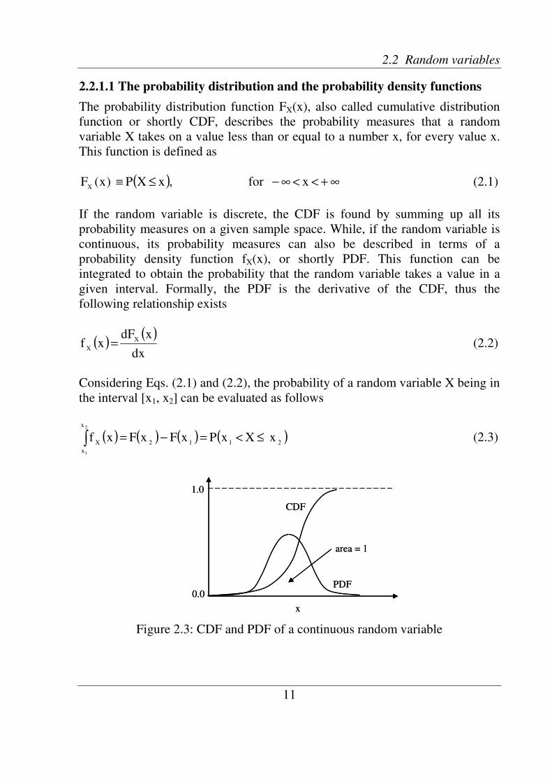
2.2.1.1 The probability distribution and the probability density functions
The probability distribution function FX(x), also called cumulative distribution
function or shortly CDF, describes the probability measures that a random
variable X takes on a value less than or equal to a number x, for every value x.
This function is defined as
( ) ∞+<<∞−≤≡ xfor,xXP)x(FX
(2.1)
If the random variable is discrete, the CDF is found by summing up all its
probability measures on a given sample space. While, if the random variable is
continuous, its probability measures can also be described in terms of a
probability density function fX(x), or shortly PDF. This function can be
integrated to obtain the probability that the random variable takes a value in a
given interval. Formally, the PDF is the derivative of the CDF, thus the
following relationship exists
( )( )
dx
xdFxf X
X= (2.2)
Considering Eqs. (2.1) and (2.2), the probability of a random variable X being in
the interval [x1, x2] can be evaluated as follows
( ) ( ) ( ) ( )2112
x
x
XxXxPxFxFxf
2
1
≤<=−=∫ (2.3)
Figure 2.3: CDF and PDF of a continuous random variable

Chapter 2 Probabilistic concepts for geotechnical engineering
12
The CDF must be a continuous non-decreasing function with values in the
interval [0,1]. As a consequence, the PDF is a non-negative function for all
values x and the total area under this function is always unity. Both functions
are plotted in Fig. 2.3.
For more detailed descriptions about the probability distribution and the
probability density functions the author refers to ANG and TANG (1975).
2.2.1.2 The mean value
The mean value of a random variable, also defined as expected or central value,
is the sum of the probability of each possible outcome of an experiment
multiplied by its value. Thus it represents the weighted average of all the
available experimental data of the variable according to the corresponding
frequency of occurrence.
In general, if X is a continuous random variable, such as the effective cohesion
of a homogeneous soil, and fX(x) is its probability density function, then its
mean value is given by
dx)x(fxXX ∫
∞+
∞−⋅=µ (2.4)
The mean value is also referred to as the first central moment, or centre of
gravity, of a probability density function, which may be, together with the
variance or second central moment, the only practically obtainable information
on soil data.
2.2.1.3 The variance and the standard deviation
Besides the mean value, another important characteristic of a random variable is
its measure of dispersion or variance, also referred to as the second central
moment, or moment of inertia, of the variable. This quantity indicates how
widely the values of the variable spread around the mean value. For a
continuous random variable X with probability density function fX(x) and using
Eq. (2.4), the variance is given by
dx)x(f)x()X(VarX
2
X
2
X⋅⋅µ−=σ= ∫
∞+
∞− (2.5)
A more understandable measure of dispersion is the standard deviation σ given
by the square root of the variance, that is

2.2 Random variables
13
)X(VarX
=σ (2.6)
As its name indicates, it gives in a standard form an indication of the possible
deviations from the mean value. It will be possible to observe in next chapters
that the standard deviation is of great importance for the evaluation of the
uncertainties of input random variables and their consequences.
2.2.1.4 The coefficient of variation
As it is hard to specify whether the dispersion of a variable is large or small only
on the basis of the standard deviation, it is more convenient to use the
coefficient of variation, or shortly COV. This non dimensional coefficient
describes whether the dispersion relative to the central value of a certain random
variable is large or small. It is defined as the ratio of the standard deviation over
the mean value of the random variable, i.e.
X
X
XCOV
µ
σ= (2.7)
Some authors have collected information on the ranges of variation coefficient
values for spatial variability of different soil properties, as derived from in-situ
soil investigation and for the variability due to measurement errors. A well-
known study on the COV values is that of PHOON and KULHAWY (1999),
which represents a good indication of the order of magnitude for the COV
values of soil variability. In this study PHOON and KULHAWY presented data
for a sand and a clay layer and they found COV values between 5-15% for the
effective friction angle. This range was also put forward by HARR (1989) and
CHERUBINI (1997). Occasionally higher COV values can be found for the
friction angle, as in the report of MOORMANN and KATZENBACH (2000),
where a value of about 30% is indicated for the Frankfurt clay. But this high
COV value of the friction angle is not for a particular site, but for the entire
Frankfurt area.
Considering the effective cohesion, HARR suggests in his work a value of
about 20%. CHERUBINI presents values between 20-30%, LI and LUMB
(1987) report a particular clay layer with a COV of 40% and MOORMANN and
KATZENBACH quote 50% for the Frankfurt clay. It can be seen that the
available data on the effective cohesion show much more variation than for the
effective friction angle.

Chapter 2 Probabilistic concepts for geotechnical engineering
14
Considering the effective cohesion, HARR suggests in his work a value of about
20%. CHERUBINI presents values between 20-30%, LI and LUMB (1987)
report a particular clay layer with a COV of 40% and MOORMANN and
KATZENBACH quote 50% for the Frankfurt clay. It can be seen that the
available data on the effective cohesion show much more variation than for the
effective friction angle.
Referring to the soil unit weight, CHERUBINI (1998) states that its variability
is rather limited (i.e. less than 10%) and for this reason this parameter will be
considered as deterministic value in this study.
However, the COV values reported in the literature for the shear strength
parameters may be considerably larger than the actual inherent soil variability.
FENTON and GRIFFITHS (2004) stated that it is still unknown which value of
the coefficient of variation should be used for the characterization of soil
parameters. In general representative values of COV are those derived from
similar geologic origins and collected over limited spatial extents of the
investigation site using good quality of equipment and procedural controls.
For this reason considerable research is needed before defining lower and
upper bounds of COV of soil properties for any given situation.
2.2.1.5 The skewness
Another useful descriptor of a random variable is the skewness or third central
moment. It is a measure of the degree of asymmetry of the probability density
function fX(x) of a random variable X. It is defined as
( ) ( )∫∞+
∞−⋅⋅µ−= dxxfx)X(skew
X
3
X (2.8)
For well-known continuous probability density functions, such as the Gaussian
distribution, formulas are available in the literature to evaluate directly the
skewness, without solving the integral (2.8).
A more convenient non-dimensional measure of asymmetry of a random
variable is the skewness coefficient given by
( )dx)x(f
xX3
X
3
X
X⋅⋅
σ
µ−=ν ∫
∞+
∞−
(2.9)
When the skewness coefficient is nil then a function is symmetric, as in the case
of a Gaussian normal distribution. Otherwise it may be positive or negative.

2.2 Random variables
15
(a)0 X
fX(x) 0X >ν
(b)0 X
fX(x) 0<νX
(a)0 X
fX(x) 0X >ν
(b)0 X
fX(x) 0<νX
Figure 2.4: Example of positively (a) and negatively (b) skewed distributions
Figure 2.5: Probability density functions of soil strength parameters for the
Frankfurt clay (MOORMANN and KATZENBACH, 2000)
Fig. 2.4(a) shows the case of a positively skewed distribution, which is steep for
low values of the random variable and flat for large values. A negatively skewed
distribution as in Fig. 2.4(b) is flat for low values of the random variable and
steep for large values. However negative skewness coefficients would seem to
be unrealistic for the distribution of soil parameters.
Considering data as reported by MOORMANN and KATZENBACH and EL
RAMLY et al. (2005), it would seem that the skewness coefficient of the
effective friction angle could be disregarded and the choice of a Gaussian
(a) (b)
freq
uen
cy
[%]
effective friction angle φ´ (°)
0
74.5
74.20
≈ν
°=σ
°=µ
ϕ′
ϕ′
ϕ′
Gaussian distribution
freq
uen
cy
[%]
effective cohesion c´ (kN/m²)
213.0
m/kN47.20
m/kN66.39
c
2
c
2
c
=ν
=σ
=µ
′
′
′
Lognormal distribution
0 5 10 15 20 25 30 35 40
40
35
30
25
20
15
10
5
0
0 5 10 15 20 25 30 35 40
40
35
30
25
20
15
10
5
0
0 10 20 30 40 50 60 70 80 90
25
20
15
10
5
0
0 10 20 30 40 50 60 70 80 90
25
20
15
10
5
0
Chapter 2 Probabilistic concepts for geotechnical engineering
16
distribution would seem suitable, as Fig. 2.5(a) shows. On the other hand, the
above authors find skewness of νc ≈1.7 (MOORMANN and KATZENB) and 4
(EL RAMLY et al.) for the effective cohesion, thus a lognormal distribution
would seem to be more appropriate, as plotted in Fig. 2.5(b). In any case, very
few data about the skewness coefficient is available in the literature and
skewness values need further testing.
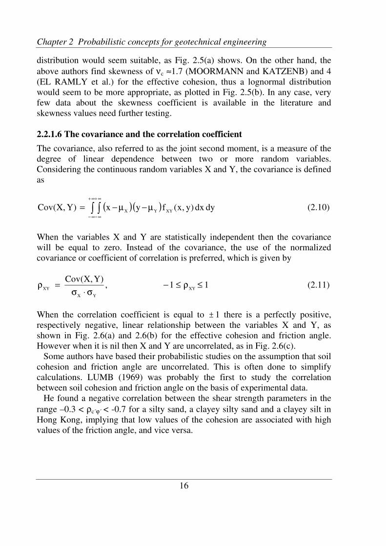
2.2.1.6 The covariance and the correlation coefficient
The covariance, also referred to as the joint second moment, is a measure of the
degree of linear dependence between two or more random variables.
Considering the continuous random variables X and Y, the covariance is defined
as
( )( )∫ ∫∞+
∞−
∞+
∞−
µ−µ−= dydx)y,x(fyx)Y,X(CovXYYX
(2.10)
When the variables X and Y are statistically independent then the covariance
will be equal to zero. Instead of the covariance, the use of the normalized
covariance or coefficient of correlation is preferred, which is given by
11,)Y,X(Cov
XY
YX
XY≤ρ≤−
σ⋅σ=ρ (2.11)
When the correlation coefficient is equal to ± 1 there is a perfectly positive,
respectively negative, linear relationship between the variables X and Y, as
shown in Fig. 2.6(a) and 2.6(b) for the effective cohesion and friction angle.
However when it is nil then X and Y are uncorrelated, as in Fig. 2.6(c).
Some authors have based their probabilistic studies on the assumption that soil
cohesion and friction angle are uncorrelated. This is often done to simplify
calculations. LUMB (1969) was probably the first to study the correlation
between soil cohesion and friction angle on the basis of experimental data.
He found a negative correlation between the shear strength parameters in the
range –0.3 < ρc´ϕ´ < -0.7 for a silty sand, a clayey silty sand and a clayey silt in
Hong Kong, implying that low values of the cohesion are associated with high
values of the friction angle, and vice versa.

2.3 Useful continuous probability distributions of random variables
17
c´
φ´
0.1´´ =ρϕc
c´
0.1´´ −=ρϕc
c´
0´´ =ρϕc
φ´φ´
(a) (b) (c)c´
φ´
0.1´´ =ρϕc
c´
0.1´´ −=ρϕc
c´
0´´ =ρϕc
φ´φ´
(a) (b) (c)
Figure 2.6: Example of perfectly positive correlated (a), perfectly negative
correlated (b) and uncorrelated (c) soil properties
However in some cases the correlation was found to be insignificant. LUMB
concluded that the assumption of independence of the strength parameters
simplifies strength interpretation considerably, and also leads to conservative
results if the correlation is in fact negative. Instead the results of CHERUBINI
(1998) indicate a significant negative correlation of ρc´ϕ´ = -0.6 between effective
cohesion and friction angle for drained triaxial tests on Blue Matera clays. The
same strong value of the correlation coefficient was reported by SCHAD (1985)
for a marl in Urbach and confirmed by SPEEDIE (1956). Hence it would seem
that a value of about -0.6 is realistic for the soil parameters.
For this reason in this study the effective cohesion and friction angle are
assumed to be negatively correlated. It will be shown that negative correlation
coefficient decreases the standard deviation of computational results, thus
increasing the reliability of the problem considered, or, inversely, decreasing the
failure probability.
2.3 Useful continuous probability distributions of random
variables
The main characteristics of a random variable can be completely described if the
probability density function and its associated parameters are known. In many
cases, unfortunately, the form of the distribution function is unknown and often
an approximated description is necessary. Several continuous distributions,
which play an important role in civil engineering as well as in numerous other
engineering fields, can be used as a good approximation for a random variable.

Chapter 2 Probabilistic concepts for geotechnical engineering
18
(a) (b)
X
6.0
5.1
=σ
=µ
X
X
75.0
5.1
=σ
=µ
X
X
0.35.20.25.10.15.00
8.0
6.0
4.0
2.0
fX(x)
Z
0.1
0.0
=σ
=µ
X
X
0.20.10.00.10.2 −−
8.0
6.0
4.0
2.0
fZ(z)
(a) (b)
X
6.0
5.1
=σ
=µ
X
X
75.0
5.1
=σ
=µ
X
X
0.35.20.25.10.15.00
8.0
6.0
4.0
2.0
fX(x)
Z
0.1
0.0
=σ
=µ
X
X
0.20.10.00.10.2 −−
8.0
6.0
4.0
2.0
fZ(z)
These continuous distributions are applied when the random variables can take
any value within some range, such as the normal and the shifted lognormal
distributions.
2.3.1 The normal and the standard normal distributions
The normal Gaussian distribution is the probability distribution most frequently
used because of its symmetry and mathematical simplicity. It is commonly
assumed to characterize many random variables where the coefficient of
variation is less than about 30%, as seen in Fig. 2.5(a) for the effective friction
angle of the Frankfurt clay.
A random variable X is said to be Gaussian normally distributed with mean
Xµ and standard deviation Xσ if its probability density function fX(x) is given by
∞<<∞−
σ
µ−⋅−⋅
σ⋅π=σµ= x,
x
2
1exp
2
1),(N(x)f
2
X
X
X
2
XXX (2.12)
In Fig. 2.7(a) the density function of the normal distribution is given for two sets
of parameters values. It can be seen that, maintaining the mean value
Xµ constant, the standard deviation Xσ governs the spread of the curves.
To simplify calculations using Eq. (2.12), an arbitrary normal distribution can
be converted to a standard normal distribution, plotted in Fig. 2.7(b), by
transforming the normal variable X into the standard normal variable Z, as
below described
Figure 2.7: Normal (a) and standard normal (b) probability density functions

2.3 Useful continuous probability distributions of random variables
19
X
XX
Zσ
µ−= (2.13)
where Z has mean 0 and standard deviation 1, i.e. N(0,1). Its corresponding
probability density function is given by
∞<<∞−
−⋅
π=Φ x,
2
zexp
2
1(z)
2
Z (2.14)
Probabilities associated with the distribution ΦZ(z) are widely tabulated in the
literature and are readily available in the software libraries of most computer
systems.
From the geotechnical point of view, the Gaussian distribution allows negative
soil properties values, which are physically unrealistic. For this reason this
distribution could never be more than a rough approximation at best.
2.3.2 The shifted and the standard lognormal distributions
A random variable X has a lognormal distribution if its natural logarithm
)ln(XY = has a normal distribution. The lognormal distribution for the random
variable X may be specified by its mean Xµ , standard deviation Xσ and
skewness coefficient Xν . Alternatively, it may be specified by the mean value
)ln(Xµ and standard deviation )ln(Xσ of the normal variable ln(X).
The general formula for the probability density function of the shifted lognormal
distribution, also defined as the three parameter lognormal distribution, is given
by
( )∞+<<
σ
µ−−−⋅
σ⋅−⋅π= xx,
)xxln(
2
1exp
xx2
1)(xf
0
2
)Xln(
)Xln(0
)Xln(0
X (2.15)
where x0 is the location or shifting parameter of the random variable X.
When this parameter is zero then one returns to the standard lognormal
distribution, which is then called two parameters lognormal distribution.
Using the shifted lognormal distribution it is possible to match not only the
mean value and standard deviation of a certain data population, as the standard
lognormal function does, but also the skewness coefficient. This allows a more
Chapter 2 Probabilistic concepts for geotechnical engineering
20
realistic data fitting. This is possible using the following closed form equations,
which allow the transformation of the lognormal random variable X into the
standard normal variable Y=ln(X):
−µ
σ+⋅−−µ=µ
2
0X
X
0X)Xln(x
1ln2
1)xln( (2.16)
−µ
σ+=σ
2
0X
X
)Xln(x
1ln (2.17)
3
0X
X
0X
X
Xxx
3
−µ
σ+
−µ
σ⋅=ν (2.18)
First of all the Eq. (2.18), which is a third degree polynomial, should be solved
numerically to get the required estimate of the location parameter x0. When the
skewness coefficient νx is nil, then Eq. (2.18) does not converge to a solution.
Once x0 is known, then the two parameters )ln(Xµ and )ln(Xσ are easily found
using Eqs. (2.16) and (2.17). For more detail about the numerical solution of
equations (2.16), (2.17) and (2.18) the reader is referred to KOTTEGODA and
ROSSO (1997).
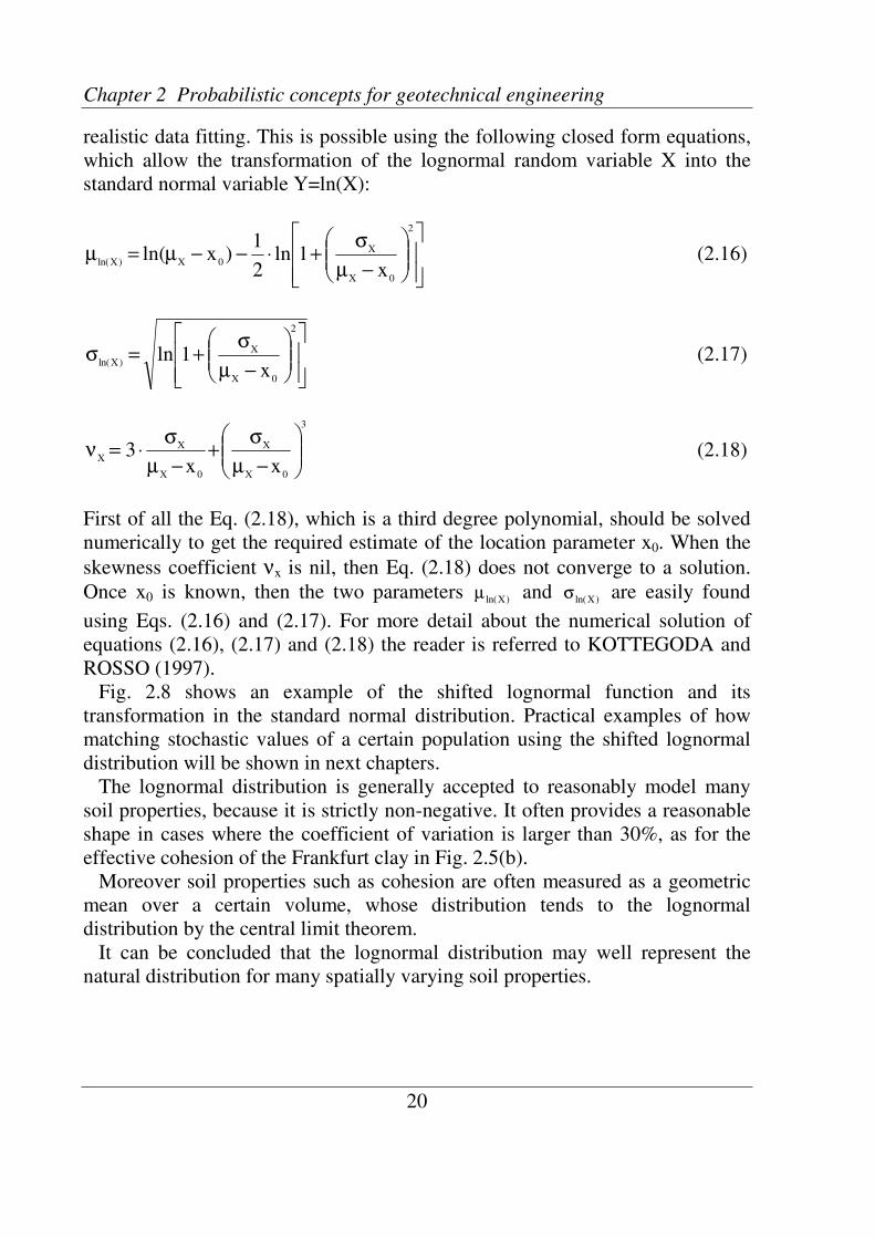
Fig. 2.8 shows an example of the shifted lognormal function and its
transformation in the standard normal distribution. Practical examples of how
matching stochastic values of a certain population using the shifted lognormal
distribution will be shown in next chapters.
The lognormal distribution is generally accepted to reasonably model many
soil properties, because it is strictly non-negative. It often provides a reasonable
shape in cases where the coefficient of variation is larger than 30%, as for the
effective cohesion of the Frankfurt clay in Fig. 2.5(b).
Moreover soil properties such as cohesion are often measured as a geometric
mean over a certain volume, whose distribution tends to the lognormal
distribution by the central limit theorem.
It can be concluded that the lognormal distribution may well represent the
natural distribution for many spatially varying soil properties.
2.4 The reliability analysis
21
9.53
7.2
50
120
0 =
=ν
=σ
=µ
x
X
X
X
X250200150100500
01.0
0075.0
005.0
0025.0
fX(x)
67.0
96.3
)ln(
)ln(
=σ
=µ
X
X
Y=ln(X)543210
8.0
6.0
4.0
2.0
fY(y)
x0
9.53
7.2
50
120
0 =
=ν
=σ
=µ
x
X
X
X
X250200150100500
01.0
0075.0
005.0
0025.0
fX(x)
67.0
96.3
)ln(
)ln(
=σ
=µ
X
X
Y=ln(X)543210
8.0
6.0
4.0
2.0
fY(y)
x0
Figure 2.8: Shifted lognormal density function and its transformation in the
standard normal distribution
2.4 The reliability analysis
One important challenge for an engineer is the definition of the safety of an
engineering project by including the uncertainty components and doing a
reliability analysis on which he can base his decisions. In order to achieve
consistent levels of reliability, which are subject to important economic and
social constraints, proper methods are required.
The object of this section is to show how the traditional safety factor relates to
the probability of failure, the latter representing a more realistic measure of a
system reliability.
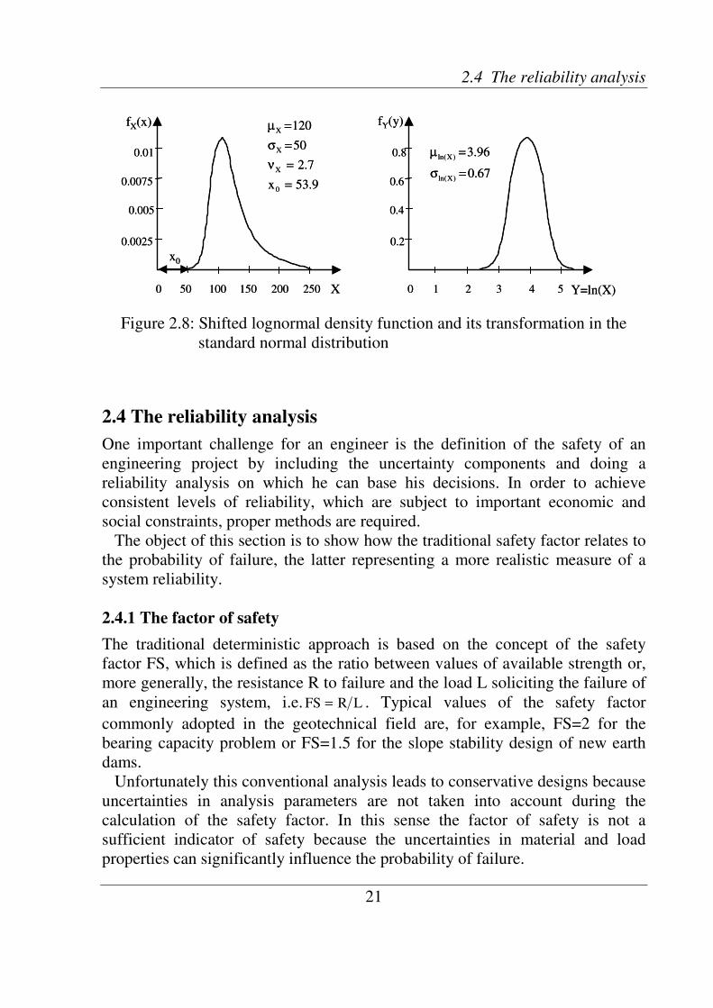
2.4.1 The factor of safety
The traditional deterministic approach is based on the concept of the safety
factor FS, which is defined as the ratio between values of available strength or,
more generally, the resistance R to failure and the load L soliciting the failure of
an engineering system, i.e. LRFS = . Typical values of the safety factor
commonly adopted in the geotechnical field are, for example, FS=2 for the
bearing capacity problem or FS=1.5 for the slope stability design of new earth
dams.
Unfortunately this conventional analysis leads to conservative designs because
uncertainties in analysis parameters are not taken into account during the
calculation of the safety factor. In this sense the factor of safety is not a
sufficient indicator of safety because the uncertainties in material and load
properties can significantly influence the probability of failure.

Chapter 2 Probabilistic concepts for geotechnical engineering
22
fX(x)
Resistance R,
Load L
FS
1fP
fX(x)
Resistance R,
Load L2fP
FS
(b) (c)
Ω
Load L
Resistance R
Z =
0
Z < 0
Z > 0
(a)
Ω
fX(x)
Resistance R,
Load L
FS
1fP
fX(x)
Resistance R,
Load L2fP
FS
(b) (c)
Ω
Load L
Resistance R
Z =
0
Z < 0
Z > 0
(a)
Ω
L L RR
fX(x)
Resistance R,
Load L
FS
1fP
fX(x)
Resistance R,
Load L2fP
FS
(b) (c)
Ω
Load L
Resistance R
Z =
0
Z < 0
Z > 0
(a)
Ω
fX(x)
Resistance R,
Load L
FS
1fP
fX(x)
Resistance R,
Load L2fP
FS
(b) (c)
Ω
Load L
Resistance R
Z =
0
Z < 0
Z > 0
(a)
Ω
L L RR
2.4.2 The safety margin and the failure probability
The traditional safety factor can be replaced by the definition of the safety
margin Z, also defined as performance function. This function could indicate the
collapse of a structure or, in a very general way, its loss of serviceability.
Figure 2.9: (a) Safety margin. (b) and (c) Safety factor versus failure probability
It is defined as the difference between the resistance R and the load L of an
engineering system. If Xi represents a collection of input random variables, then
the safety margin is given by
( ) ( ) ( )iii
XLXRXZ −= (2.19)
In Fig. 2.9(a) the safety margin is plotted and the failure space is indicated in the
Resistance-Load-plane. When Z<0 then failure occurs, while when Z>0 then the
system is safe. The boundary defined by Z=0 separating the safe and unsafe state
is called the limit state function.
The goal of the reliability analysis is the assurance of safety and this is
possible only in terms of probability, i.e.
( )( ) ( ) ( )( )iiiS
XLXRP0XZPP >=>= (2.20)
where ( ) ( )( )ii XLXRP > is the probability that the resistance is greater than the
load. On the other hand the probability of unsafe conditions or failure
probability is given by
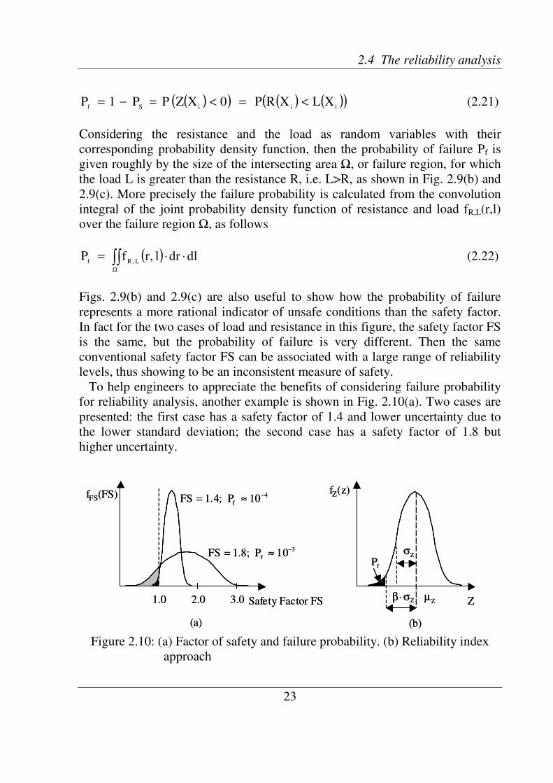
2.4 The reliability analysis
23
fFS(FS)
Safety Factor FS1.0 2.0 3.0
410;4.1 −≈= fPFS
310;8.1 −≈= fPFS
(a)
fZ(z)
ZZµZσ⋅β
Zσ
fP
(b)
fFS(FS)
Safety Factor FS1.0 2.0 3.0
410;4.1 −≈= fPFS
310;8.1 −≈= fPFS
(a)
fZ(z)
ZZµZσ⋅β
Zσ
fP
(b)
( )( ) ( ) ( )( )iiiSf
XLXRP0XZPP1P <=<=−= (2.21)
Considering the resistance and the load as random variables with their
corresponding probability density function, then the probability of failure Pf is
given roughly by the size of the intersecting area Ω, or failure region, for which
the load L is greater than the resistance R, i.e. L>R, as shown in Fig. 2.9(b) and
2.9(c). More precisely the failure probability is calculated from the convolution
integral of the joint probability density function of resistance and load fR,L(r,l)
over the failure region Ω, as follows
( ) dldrl,rfPL,Rf
⋅⋅= ∫∫Ω
(2.22)
Figs. 2.9(b) and 2.9(c) are also useful to show how the probability of failure
represents a more rational indicator of unsafe conditions than the safety factor.
In fact for the two cases of load and resistance in this figure, the safety factor FS
is the same, but the probability of failure is very different. Then the same
conventional safety factor FS can be associated with a large range of reliability
levels, thus showing to be an inconsistent measure of safety.
To help engineers to appreciate the benefits of considering failure probability
for reliability analysis, another example is shown in Fig. 2.10(a). Two cases are
presented: the first case has a safety factor of 1.4 and lower uncertainty due to
the lower standard deviation; the second case has a safety factor of 1.8 but
higher uncertainty.
Figure 2.10: (a) Factor of safety and failure probability. (b) Reliability index
approach

Chapter 2 Probabilistic concepts for geotechnical engineering
24
From a deterministic point of view it would seem that the case with FS=1.8 is
safer. However when one compares the failure probability values, then the
apparently safer case has a higher probability of failure, thus demonstrating that
the deterministic analysis is not always safe against failure.
It can be concluded that, while one does not precisely know what a safety
factor of 1.5 means, a failure probability, for example, of 10-3
is very clear.
2.4.3 The reliability index
If resistance and load follow normal distributions then the convolution integral
(2.22) may be evaluated as
( )β−Φ=βΦ−= )(1Pf
(2.23)
where Φ denotes the standard normal distribution function and β is a very useful
parameter for characterizing the degree of safety, commonly called the
reliability index. This index was first defined by CORNELL (1969) and is given
by
Z
Z
LRRL
2
L
2
R
LR
2)normal(
σ
µ=
σ⋅σ⋅ρ⋅±σ+σ
µ−µ=β (2.24)
where µR, µL and µZ, respectively σR, σL and σZ are the mean values,
respectively the standard deviations of resistance, load and safety margin. While
ρRL is the correlation coefficient between resistance and load. In the case of
uncorrelated input variables the term with the correlation coefficient drops out.
As Fig. 2.10(b) shows, the reliability index represents the number of standard
deviations of the safety margin Z by which the mean value µZ exceeds the limit
state.
Figure 2.11 shows the relation between failure probability and reliability index
for a performance function with a normal distribution. It is clear how the
reliability index is monotonically related to the failure probability, so that higher
values of β imply lower values of Pf. Other distributions give similar curves for
β<2.5, but the curves differ substantially for higher values of the reliability
index.
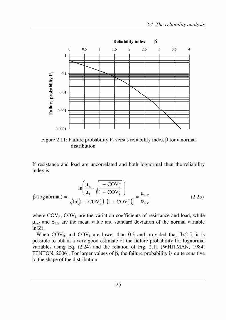
2.4 The reliability analysis
25
0.0001
0.001
0.01
0.1
1
0 0.5 1 1.5 2 2.5 3 3.5 4
Reliability index
Fa
ilu
re p
roba
bil
ity
Pf
β
0.0001
0.001
0.01
0.1
1
0 0.5 1 1.5 2 2.5 3 3.5 4
Reliability index
Fa
ilu
re p
roba
bil
ity
Pf
β
Figure 2.11: Failure probability Pf versus reliability index β for a normal
distribution
If resistance and load are uncorrelated and both lognormal then the reliability
index is
( ) ( )[ ] Zln
Zln
2
L
2
R
2
R
2
L
L
R
COV1COV1ln
COV1
COV1ln
)normal(logσ
µ=
+⋅+
+
+⋅
µ
µ
=β (2.25)
where COVR, COVL are the variation coefficients of resistance and load, while
µlnZ and σlnZ are the mean value and standard deviation of the normal variable
ln(Z).
When COVR and COVL are lower than 0.3 and provided that β<2.5, it is
possible to obtain a very good estimate of the failure probability for lognormal
variables using Eq. (2.24) and the relation of Fig. 2.11 (WHITMAN, 1984;
FENTON, 2006). For larger values of β, the failure probability is quite sensitive
to the shape of the distribution.


27
Chapter 3
Probabilistic methods for quantifying
uncertainties in Geotechnics
Introduction The quantification and analysis of uncertainty are central issues in the evaluation
of reliability and the development of associated reliability based-design.
The purpose of this chapter is to review some well-known probabilistic
techniques, such as the Monte Carlo and the Point Estimate methods, for dealing
with uncertainties and for implementing probabilistic concepts into geotechnical
analyses in a more rational way. Actually, assuming soil parameters, such as the
friction angle and the cohesion, as random variables described by a certain
probability density function, then probabilistic methods are applied to assess the
probability density function and the statistical values of a limit state function
(e.g. the bearing capacity) which depends on the input variables. Thus, failure
probabilities and reliability indeces can be estimated from the output results,
leading to a more meaningful evaluation of safety design.
In this chapter the methodology of probabilistic approaches are illustrated and
their corresponding advantages and limitations discussed.
3.1 Monte Carlo Simulations (MCS)
The word “simulation” refers to any numerical method meant to imitate a real-
life system, especially when other analyses are mathematically too complex or
too difficult to reproduce. Without the aid of simulation, a spreadsheet model
will only reveal a single deterministic outcome, generally the most likely or
average value. One type of simulation technique is the Monte Carlo method,
which can be used in every field, from economics to nuclear physics. Of course
the way this method is applied varies widely from field to field. In the MCS
assumptions are only made on the input random variables, whose values are
generated consistently with the corresponding probability

Chapter 3 Probabilistic methods for quantifying uncertainties in Geotechnics
28
density function. Then the safety margin, for which no assumption on the
probability density function is required, is calculated for each realization. The
process is repeated numerous times, typically thousands, and the mean value,
standard deviation, skewness coefficient and probability distribution of the
safety margin are evaluated. Thus Monte Carlo procedure consists of solving a
deterministic problem many times to build up a statistical distribution of the
output.
This method is close to the real answer and is therefore used as reference for
comparison with other probabilistic methods results, as will be shown in the
following chapters for the probabilistic analysis of the bearing capacity problem.
However, for certain geotechnical problems, such as slope stability analyses,
additional special programming for the MCS would be needed. Moreover, to
obtain any real confidence, the model would need a large number of simulations.
In practice, it is too time consuming for daily computer calculations, especially
for Finite Elements codes. The idea is, therefore, to replace MCS by other
probabilistic approaches requiring only a limited amount of calculations.
For more detail about MCS and the way of generating random numbers, the
author refers to ANG and TANG (1984), ROSS (1995) and the publication
CUR190 of the Delft University of Technology (CUR-Publicatie 190, 1997).
3.2 The First Order Second Moment method (FOSM)
The first relatively simple alternative to MCS is the well-known First Order
Second Moment method, or shortly FOSM, which produces a linearisation
around the mean value of the input random variables of a probabilistic problem.
This method uses a Taylor’s series expansion of the performance function to be
evaluated to determine the values of its first two central moments, mean value
and standard deviation, depending on the input variables. This expansion is
truncated after the linear term and, for this reason, the method is called “First
Order”.
Considering a performance function Z of n random variables Xi, as for
example the bearing capacity as function of the cohesion and the friction angle,
its Taylor’s series expansion about the mean value of the random variables
µX1,…, µXn, truncated after first order terms, gives
( )i
n
1iXiXXn1
x
ZX)...,,(Z)X,...,X(Z
in1
∂
∂⋅µ−+µµ= ∑
=
(3.1)

3.2 The First Order Second Moment method (FOSM)
29
The derivatives are evaluated at µX1,…, µXn, considered as linearisation points.
The mean value and the variance of the performance function are given
approximately by the following equations
( ))...,,(Z
n1n1 xxx,...,xZµµ≈µ (3.2)
( ) ( )ji
n
1jji
n
1ii
2n
1ii
n1X,XCov
x
Z
x
Z2XVar
x
Z])X...,,X(Z[Var ⋅
∂
∂⋅
∂
∂⋅+⋅
∂
∂≈ ∑∑∑
===
(3.3)
If the random variables are uncorrelated, then the term with the covariance drops
out. In general, for n random variables 2n+1 calculations are involved.
In practice it is sometimes complicated to evaluate derivatives of non-linear
functions. For this reason the required derivatives can be estimated numerically
using the finite difference approach, described in detail by EL-RAMLY,
MORGENSTERN and CRUDEN (2001).
The usual output of FOSM method is the reliability index given by Eq. (2.24)
for normally distributed variables. For non-normal probability density functions
the reliability index evaluated by FOSM method is only an approximation. Very
refined methods have been developed to convert general probability density
functions into standard normal distributions (ANG and TANG, 1984).
3.2.1 Advantages and limitations of the FOSM method
The most important advantages of the FOSM method include the following:
• The FOSM method is exact for linear performance functions.
• The summation terms of Eqs. 3.1 and 3.3 provide an explicit indication of
the relative contribution of uncertainty of each random variable.
• Experts (EL RAMLY, MORGENSTERN and CRUDEN, 2003) state that,
in comparison to MCS, the FOSM method shows an error in its estimates
between 5%-15%, which is a reasonable value for geotechnical field. This
will be shown in next chapters.
To avoid the misuse of FOSM method in probabilistic analyses, one should be
referred of its limitations, which are listed below:
• Due to the Taylor’s series truncation after first order terms, the accuracy
of the method deteriorates if second and higher derivatives of the

Chapter 3 Probabilistic methods for quantifying uncertainties in Geotechnics
30
performance function are significant. Thus the accuracy of the FOSM
method diminishes as the non-linearity of a function increases.
Unfortunately, retaining second and higher order terms of the Taylor’s
series expansion of a complex function with more than one input variable
is mathematically complex.
• The skewness of the output probability density function is not provided.
• As the level of uncertainty in the input variables increases and their
probability density functions become more skewed the accuracy of the
FOSM method decreases.
• Additional assumptions on the output probability density function must be
made to estimate any probability of failure; moreover the reliability index
is not uniquely defined, because it depends on the safety format
considered (e.g. R-L=0, where R = resistance and L = load).
• The shape of the probability density function of the input variables is not
taken into account, the random variables are described using only their
mean and standard deviation. In this way no information about the shape
of the probability density function of the output is provided, but it has to
be assumed. This assumption introduces a source of inaccuracy.
• Finally, the FOSM method is applied primarily to problems without
spatial correlation among input variables. With extra calculation effort,
the method can be applied for two correlated random variables, but this
can be very cumbersome.
3.3 The Second Order Second Moment method (SOSM)
The Second Order Second Moment method, or shortly SOSM, represents a
slight extension of FOSM method. Actually with SOSM method it is possible to
include second order terms of the Taylor’s series expansion in the evaluation of
the mean value of a performance function.
Considering the variances, or standard deviations, of two random variables X,
Y as known, the mean value of Z(X,Y) is given by
( )( ) ( ) ( ) ( ) ( )
yx
ZY,XCov
y
ZYVar
2
1
x
ZXVar
2
1
y
Zy
x
Zx),(Z
2
2
2
2
2
YXYXY,XZ∂⋅∂
∂⋅+
∂
∂⋅⋅+
∂
∂⋅⋅+
∂
∂⋅µ−+
∂
∂⋅µ−+µµ≈µ
(3.4)
where all derivatives are evaluated at the mean value of the input variables. The
term including the covariance drops out if the variables are uncorrelated.

3.4 The Hasofer Lind method (FORM)
31
(a) (b)
Resistance R
Load L Z = 0
Z < 0Z > 0
design point PUR
UL
design point PZ = 0
Z < 0
Z > 0 β
Rµ
Lµ
(a) (b)
Resistance R
Load L Z = 0
Z < 0Z > 0
design point PUR
UL
design point PZ = 0
Z < 0
Z > 0 β
Rµ
Lµ
When compared with FOSM method, the obvious advantage of SOSM method
is that the calculated mean value is more accurate because second order terms
are considered in the analysis.
Important references for FOSM and SOSM methods and their applications to
engineering problems are: GRIFFITHS, FENTON and TVETEN (2002),
CHRISTIAN and BÄCHER (1992, 1994), MOSTYN and LI (1993), WOLFF
(1994), DUNCAN (2000).
3.4 The Hasofer-Lind method (FORM)
A drawback of the FOSM method is that the results depend on the mean value
of the input variables at which the partial derivatives of the safety margin are
evaluated (invariance problem). Moreover the FOSM method is exact only for
linear functions, while for non-linear functions errors are introduced in the
analysis.
The Hasofer-Lind method, also well-known as the First Order Reliability
Method, or shortly FORM, can overcome this difficulty by calculating the
derivatives of the safety margin at a critical point on the failure surface, also
called design point. An iterative solution is usually required to find this point,
but the process tends to converge very rapidly.
Figure 3.1: Linearisation of the safety margin in the design point in the RL-plane
(a) and definition of the reliability index for normalized random
variables (b)
l
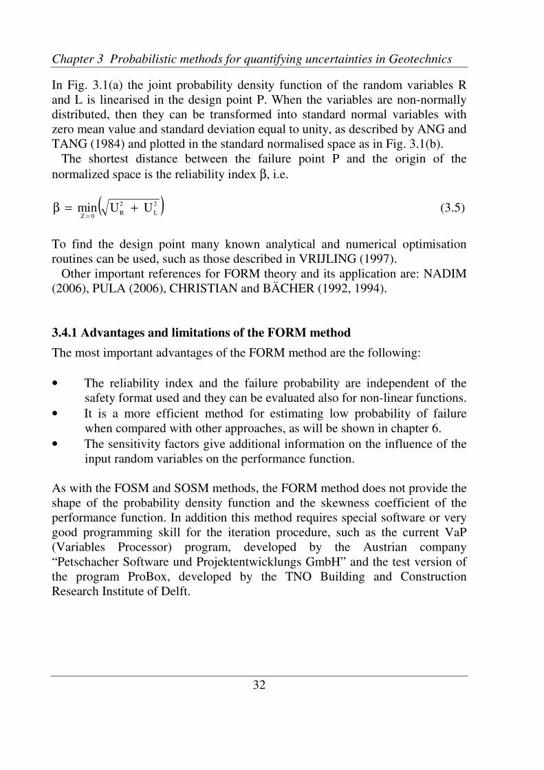
Chapter 3 Probabilistic methods for quantifying uncertainties in Geotechnics
32
In Fig. 3.1(a) the joint probability density function of the random variables R
and L is linearised in the design point P. When the variables are non-normally
distributed, then they can be transformed into standard normal variables with
zero mean value and standard deviation equal to unity, as described by ANG and
TANG (1984) and plotted in the standard normalised space as in Fig. 3.1(b).
The shortest distance between the failure point P and the origin of the
normalized space is the reliability index β, i.e.
( )2
L
2
R0Z
UUmin +=β=
(3.5)
To find the design point many known analytical and numerical optimisation
routines can be used, such as those described in VRIJLING (1997).
Other important references for FORM theory and its application are: NADIM
(2006), PULA (2006), CHRISTIAN and BÄCHER (1992, 1994).
3.4.1 Advantages and limitations of the FORM method
The most important advantages of the FORM method are the following:
• The reliability index and the failure probability are independent of the
safety format used and they can be evaluated also for non-linear functions.
• It is a more efficient method for estimating low probability of failure
when compared with other approaches, as will be shown in chapter 6.
• The sensitivity factors give additional information on the influence of the
input random variables on the performance function.
As with the FOSM and SOSM methods, the FORM method does not provide the
shape of the probability density function and the skewness coefficient of the
performance function. In addition this method requires special software or very
good programming skill for the iteration procedure, such as the current VaP
(Variables Processor) program, developed by the Austrian company
“Petschacher Software und Projektentwicklungs GmbH” and the test version of
the program ProBox, developed by the TNO Building and Construction
Research Institute of Delft.

3.5 The Two Point Estimate Method (PEM)
33
3.5 The Two Point Estimate Method (PEM)
Another alternative method to evaluate statistical moments of a performance
function is the Point Estimate Method, or shortly PEM. The Point Estimate
method was first developed by ROSENBLUETH (1975, 1981) and then further
developed by other authors such as CHRISTIAN and BÄCHER (1999), EVANS
et al. (1993), LIND (1983), ZHOU and NOWAK (1988), HARR (1989), LI
(1992), HONG (1998). The method used in this study is the “Two Point
Estimate Method” after ROSENBLUETH.
The Two Point Estimate method is a computationally straightforward
technique for uncertainty analysis, capable of estimating statistical moments of a
model output involving several stochastic variables, correlated or uncorrelated,
symmetric or asymmetric. It is fundamentally a weighted average method
similar to numerical integration formulas involving sampling points and
weighting parameters.
The PEM can be seen as a special case of the orthogonal polynomial
approximation procedures leading to the Gaussian quadrature formulas, which
are well known in numerical analyses and in Finite Elements methods
(CHRISTIAN and BÄCHER, 1999).
The basic idea of this method is to replace the probability distributions of
continuous random variables by discrete equivalent distributions having the
same first three central moments, to calculate then the mean value, standard
deviation and skewness of a performance function, which depends on the input
variables.
To do this, two point estimates are considered at one standard deviation on
either side of the mean value from each distribution representing the random
variables. Then the performance function is calculated for every possible
combination of the point estimates, producing 2n solutions, where n is the
number of the random variables involved. Then the mean value, standard
deviation and skewness of the performance function can be found from these 2n
solutions.
While the PEM does not provide a full distribution of the output variable, as
Monte Carlo does, it requires little knowledge of probability concepts and could
be applied for any probability distribution. In future it might be widely used for
reliability analysis and for the evaluation of failure probability of engineering
systems.
The procedure for implementing the PEM is clearly described in the next
section. For a simple introduction, the reader should refer to GRIFFITHS,
FENTON and TVETEN (2002).
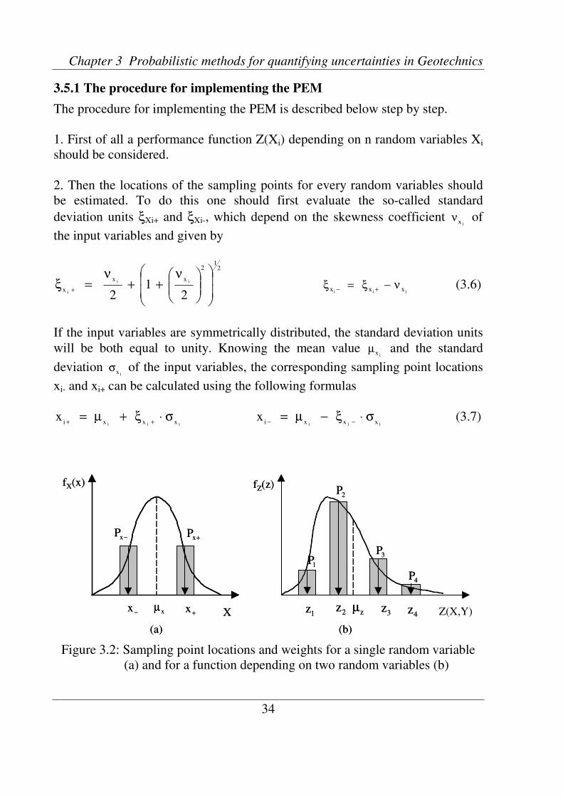
Chapter 3 Probabilistic methods for quantifying uncertainties in Geotechnics
34
X−x
+x
fX(x)
−xP+xP
xµ Z(X,Y)1z 2z zµ
1P
2P
3z4z
3P
4P
fZ(z)
(a) (b)
X−x
+x
fX(x)
−xP+xP
xµ Z(X,Y)1z 2z zµ
1P
2P
3z4z
3P
4P
fZ(z)
(a) (b)
3.5.1 The procedure for implementing the PEM
The procedure for implementing the PEM is described below step by step.
1. First of all a performance function Z(Xi) depending on n random variables Xi
should be considered.
2. Then the locations of the sampling points for every random variables should
be estimated. To do this one should first evaluate the so-called standard
deviation units ξXi+ and ξXi-, which depend on the skewness coefficient ixν of
the input variables and given by
21
2
xx
x2
12
ii
i
ν++
ν=ξ
+
iii xxx ν−ξ=ξ+−
(3.6)
If the input variables are symmetrically distributed, the standard deviation units
will be both equal to unity. Knowing the mean value ixµ and the standard
deviation ixσ of the input variables, the corresponding sampling point locations
xi- and xi+ can be calculated using the following formulas
iii xxxix σ⋅ξ+µ=
++
iii xxxix σ⋅ξ−µ=
−− (3.7)
Figure 3.2: Sampling point locations and weights for a single random variable
(a) and for a function depending on two random variables (b)
3.5 The Two Point Estimate Method (PEM)
35
In Fig. 3.2(a) and 3.2(b) the sampling point locations for a single random
variable and for a function Z depending on two random variables X and Y are
shown.
3. The weights Pi, also called probability concentrations, can now be determined
to obtain all the point estimates. As a probability density function encloses an
area of unity, then the weights must also sum to unity and they have to be
positive. The weights of the random variables are given by different expressions
depending on the number of the input variables and on their correlation. An
example of weights distribution is shown in Fig. 3.2(a) and 3.2(b).
For a single random variable (ROSENBLUETH, 1975) the weights are easily
calculated using the standard deviation units as
−+
−
+
ξ+ξ
ξ=
xx
x
xP
+−−=
xxP1P (3.8)
When the random variable is symmetric then the weights are both equal to 0.5,
as shown in Fig. 3.2(a).
For two correlated random variables (ROSENBLUETH, 1981) the weights are
given as follows
ν+⋅
ν+ρ⋅⋅+⋅=
21
3
x
3
x
xx21xxss2
12
1/ssPPP 21
212s1s21 (3.9)
where 2s1s XX
PP ⋅ are the associated weights, with 1sX
P and 2sX
P being the weights
for the input variables evaluated as single variables. 21 xx
ρ is the correlation
coefficient between the variables X1 and X2, s1 and s2 take positive sign for
points greater than the mean value of the variables and negative sign for points
smaller than the mean value.
The sign product 21
ss ⋅ determines the sign of the correlation coefficient and
the subscripts of the weight P indicate the location of the point that is being
weighted. For example, considering the point evaluated at
( ) ( )222111 xxxxxx21
,x,x σ⋅ξ−µσ⋅ξ+µ=−+−+
then s1 = + and s2 = -, resulting in
a negative product with a weight denoted by P+-.

Chapter 3 Probabilistic methods for quantifying uncertainties in Geotechnics
36
When the variables are uncorrelated then 21 xx
ρ will be zero and the formula
(3.9) will give the associated weights of two uncorrelated random variables.
Unfortunately Eq. (3.9) has some evident drawbacks. First of all, if the
skewness coefficient of the input variables has different sign then the radicand
under the square root can be negative, which is mathematically impossible. This
can happen for example if one input variable has a negatively skewed
distribution and the other a symmetrically or positively skewed distribution.
Secondly if the skewness coefficient of the input variables is equal to –2 then the
denominator of the second term of Eq. (3.9) tends to infinity, giving then infinite
weights. Moreover this formula can sometimes give negative values. This fact is
unacceptable, because the weights are described as probability values, which are
always positive by definition. For example, negative values of the weights can
occur when the random variables are symmetric and perfectly correlated (i.e.
121 xx
±=ρ ).
The problem of obtaining negative weights could be solved, for example, by
applying the Three Points Estimate Method instead of the Two PEM.
Considering all the drawbacks of Eq. (3.9), it is necessary to establish some
conditions for its use, i.e.
1)
ν+⋅
ν+ρ⋅⋅>⋅
21
3
x
3
x
xx21xx2
12
1/ssPP 21
212s1s (3.10)
2) 02
12
1
3
x
3
x 21
>
ν+⋅
ν+ (3.11)
3) 21x
−≠ν and/or 22x
−≠ν (3.12)
The first condition assures that the weights are positive. The third condition is
actually already implied in the second one.
To overcome the problem in ROSENBLUETH’s formula (3.9), a better
definition for two correlated random variables, being symmetrically distributed,
is given by CHRISTIAN et al. (1999), where the weights can be evaluated as
( )2121 XXxx
1PPPP ρ−⋅⋅==±+−−+
m
( )2121 XXxx
1PPPP ρ+⋅⋅==±±++−−
(3.13)
3.5 The Two Point Estimate Method (PEM)
37
For n symmetrically distributed and correlated random variables, CHRISTIAN
et al. (1999) define the weights as
( )
ρ⋅⋅+⋅= ∑ ∑
−
= +=
1n
1i
n
1ijijjins...ss
ss12
1P
n21 (3.14)
In equation (3.14) the notation is the same as for equation (3.9).
4. Now it is possible to determine the performance function Z(Xi) at each
sampling point located at xi+ and xi-. To do this, it is sufficient to introduce the
sampling point estimates found using Eqs. (3.7) in the formula of the
performance function. For n random variables, the performance function is
evaluated at 2n points.
5. Finally the first three moments of the performance function, respectively the
mean value, the variance and the skewness coefficient, can be determined using
the following equations
( )( )∑
=
=⋅=µ
n
i
2
1iiiiXZ
xXZP (3.15)
( ) ( )( )
( )2
2
1iXZiiiXZ
2
n
ii xXZP∑
=
µ−=⋅=σ (3.16)
( )
( )
( )( )
( )3
2
1iXZiii3
XZ
XZ
n
i
i
ixXZP
1∑
=
µ−=⋅σ
=ν (3.17)
The standard deviation of the performance function is easily obtained as
( )( )
( )( )∑
=
µ−=⋅=σ
n
ii
2
1i
2
XZiiiXZxXZP (3.18)
ROSENBLUETH (1981) notes that for the multiple random variables case,
skewness coefficients can only be reliably calculated using Eq. (3.17) if the
variables are uncorrelated. This fact will be shown in chapter 5.
3.5.2 Advantages and limitations of the PEM
The most important advantages of PEM in comparison to FOSM, SOSM and
FORM methods are:

Chapter 3 Probabilistic methods for quantifying uncertainties in Geotechnics
38
• As with the FOSM, SOSM and FORM methods, the PEM does not
require the knowledge of the particular shape of the probability density
function of the input random variables. Moreover the PEM furnishes the
exact solution for linear performance functions.
• It provides not only the mean value and the standard deviation, but also
the skewness coefficient of a performance function, giving then more
accurate results than FOSM, SOSM and FORM methods, with little or no
increase in computational effort.
• The PEM may better capture the behaviour of non-linear functions.
• To evaluate the statistical values of a performance function there is no
need to compute the derivatives, nor even their continuity let alone their
existence.
• As a non-iterative procedure, the PEM overcomes the convergence
problems of the FORM, thus being less time consuming.
• It can be also applied to problems with spatial correlation among multiple
input variables, even if more computational effort is required.
When compared with Monte Carlo method, the PEM results in terms of mean
value and standard deviation are in good agreement with those of MCS, with
smaller computational effort for a comparable degree of accuracy.
Limitations of the PEM as described above:
• No information about the shape of the probability density function of the
output is provided, but it has to be assumed, introducing uncertainty in the
final results.
• The skewness provided by PEM presents a significant difference to the
skewness value derived from MCS, as it will be shown in chapter 5.
• If more accuracy is required, then a larger number of input variables is
necessary and higher moments have to be considered, thus increasing the
number of calculations.
• Results are poor and less accurate for discontinuous functions or functions
having discontinuous first derivatives (CHRISTIAN and BÄCHER,
1999).
• The implementation of PEM into Finite Element codes requires additional
out of house software.
• CHRISTIAN and BÄCHER (1999) suggest that the PEM should not be
applied for evaluating moments higher than the second (i.e. variance) for
non-linear functions. Additionally they observe that the larger the
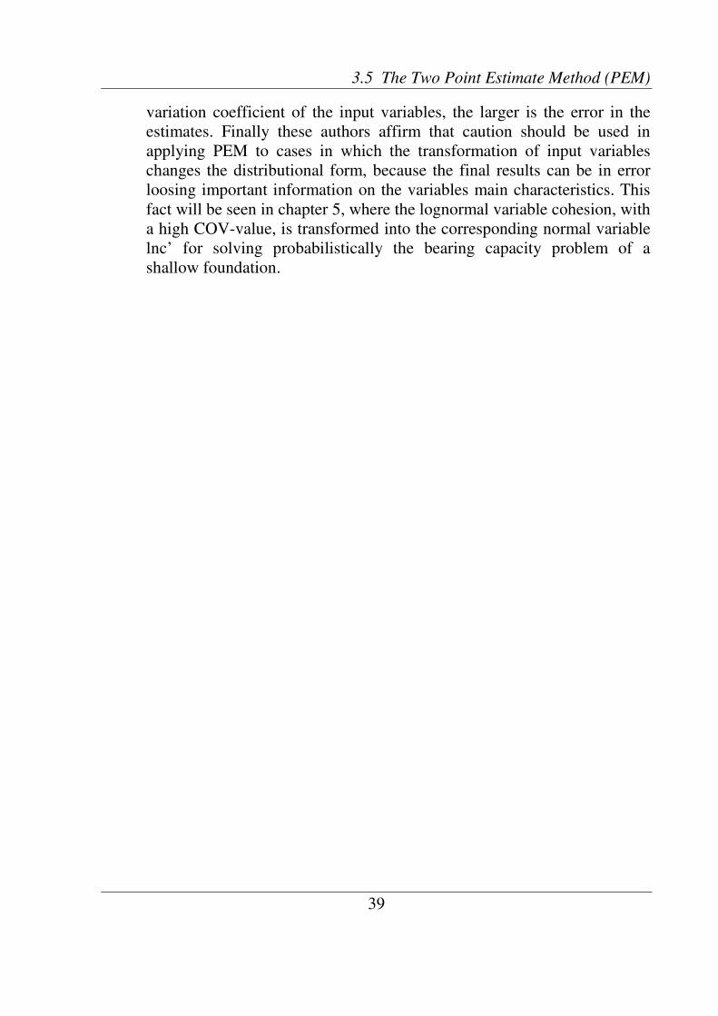
3.5 The Two Point Estimate Method (PEM)
39
variation coefficient of the input variables, the larger is the error in the
estimates. Finally these authors affirm that caution should be used in
applying PEM to cases in which the transformation of input variables
changes the distributional form, because the final results can be in error
loosing important information on the variables main characteristics. This
fact will be seen in chapter 5, where the lognormal variable cohesion, with
a high COV-value, is transformed into the corresponding normal variable
lnc’ for solving probabilistically the bearing capacity problem of a
shallow foundation.


41
Chapter 4
Probabilistic analysis of the bearing
capacity problem
Introduction This chapter presents an application of probabilistic methods to the study of the
bearing capacity of a strip footing on a homogeneous soil layer characterised by
the effective cohesion c´ and friction angle ϕ´. These parameters are selected to
be represented as random variables since they have the greatest impact on the
soil bearing capacity.
Different values of the correlation coefficient between soil parameters are
taken into account in the analysis. The influence of the spatial variability of soil
parameters (i.e. the scale of fluctuation), which is a significant source of error, is
ignored here.
For a comparison of the failure probabilities from the MCS, FOSM and SOSM
methods the author refers to chapter 6.
4.1 Benchmarks on the bearing capacity of a strip footing
4.1.1 Benchmark 1: bearing capacity of a strip footing with effective friction
angle as the input random variable
The first benchmark deals with the study of the bearing capacity of a strip
footing with a width of 2m on top of a cohesionless homogeneous soil layer, as
shown in Fig. 4.1(a). More specifically, the soil type is what can be called a
grossly uniform soil, in which the whole mass is all of the same consistency and
whose properties show no marked trend with depth or distance.
For this study soil layering is ignored, assuming that in the soil mass no
discontinuities or sudden changes exist. The unit soil weight is 15 kN/m3 and a
surcharge q0=10 kN/m2 is considered. The effective soil cohesion c´ is taken as a
uniform fixed property with a value of 4 kN/m2, while the effective friction
angle ϕ´ is taken into account as a normal random variable with its
corresponding statistical values given in Fig. 4.1(b).
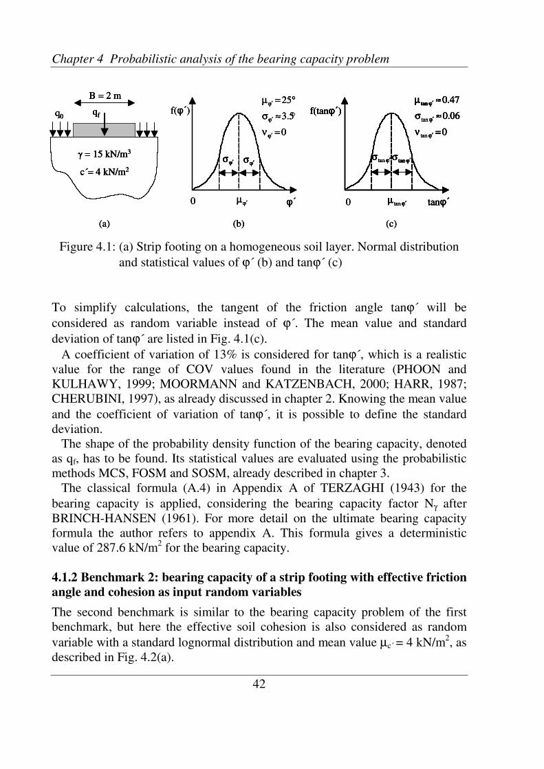
Chapter 4 Probabilistic analysis of the bearing capacity problem
42
γ = 15 kN/m3
c´= 4 kN/m2
qf
B = 2 m
q0
(a) (b)
f(φ´)
φ´
0
5.3
25
=ν
≈σ
°=µ
ϕ′
ϕ′
ϕ′
ϕ′µ
ϕ′σϕ′σϕ′σϕ′σ
0
(c)
f(tanφ´)
tanφ´ϕ′µ tan
0
06.0
47.0
tan
tan
tan
=ν
≈σ
≈µ
ϕ′
ϕ′
ϕ′
ϕ′σ tan ϕ′σ tan
f(tanφ´)
tanφ´ϕ′µ tan
0
06.0
47.0
tan
tan
tan
=ν
≈σ
≈µ
ϕ′
ϕ′
ϕ′
ϕ′σ tan ϕ′σ tan
0
°
γ = 15 kN/m3
c´= 4 kN/m2
qf
B = 2 m
q0
(a)
γ = 15 kN/m3
c´= 4 kN/m2
qf
B = 2 m
q0
γ = 15 kN/m3
c´= 4 kN/m2
qf
B = 2 m
q0
(a) (b)
f(φ´)
φ´
0
5.3
25
=ν
≈σ
°=µ
ϕ′
ϕ′
ϕ′
ϕ′µ
ϕ′σϕ′σϕ′σϕ′σ
0
(b)
f(φ´)
φ´
0
5.3
25
=ν
≈σ
°=µ
ϕ′
ϕ′
ϕ′
ϕ′µ
ϕ′σϕ′σϕ′σϕ′σ
0
(c)
f(tanφ´)
tanφ´ϕ′µ tan
0
06.0
47.0
tan
tan
tan
=ν
≈σ
≈µ
ϕ′
ϕ′
ϕ′
ϕ′σ tan ϕ′σ tan
f(tanφ´)
tanφ´ϕ′µ tan
0
06.0
47.0
tan
tan
tan
=ν
≈σ
≈µ
ϕ′
ϕ′
ϕ′
ϕ′σ tan ϕ′σ tan
0
(c)
f(tanφ´)
tanφ´ϕ′µ tan
0
06.0
47.0
tan
tan
tan
=ν
≈σ
≈µ
ϕ′
ϕ′
ϕ′
ϕ′σ tan ϕ′σ tan
f(tanφ´)
tanφ´ϕ′µ tan
0
06.0
47.0
tan
tan
tan
=ν
≈σ
≈µ
ϕ′
ϕ′
ϕ′
ϕ′σ tan ϕ′σ tan
0
°
Figure 4.1: (a) Strip footing on a homogeneous soil layer. Normal distribution
and statistical values of ϕ´ (b) and tanϕ´ (c)
To simplify calculations, the tangent of the friction angle tanϕ´ will be
considered as random variable instead of ϕ´. The mean value and standard
deviation of tanϕ´ are listed in Fig. 4.1(c).
A coefficient of variation of 13% is considered for tanϕ´, which is a realistic
value for the range of COV values found in the literature (PHOON and
KULHAWY, 1999; MOORMANN and KATZENBACH, 2000; HARR, 1987;
CHERUBINI, 1997), as already discussed in chapter 2. Knowing the mean value
and the coefficient of variation of tanϕ´, it is possible to define the standard
deviation.
The shape of the probability density function of the bearing capacity, denoted
as qf, has to be found. Its statistical values are evaluated using the probabilistic
methods MCS, FOSM and SOSM, already described in chapter 3.
The classical formula (A.4) in Appendix A of TERZAGHI (1943) for the
bearing capacity is applied, considering the bearing capacity factor Nγ after
BRINCH-HANSEN (1961). For more detail on the ultimate bearing capacity
formula the author refers to appendix A. This formula gives a deterministic
value of 287.6 kN/m2 for the bearing capacity.
4.1.2 Benchmark 2: bearing capacity of a strip footing with effective friction
angle and cohesion as input random variables
The second benchmark is similar to the bearing capacity problem of the first
benchmark, but here the effective soil cohesion is also considered as random
variable with a standard lognormal distribution and mean value µc´ = 4 kN/m2, as
described in Fig. 4.2(a).

4.1 Benchmarks on the bearing capacity of a strip footing
43
Figure 4.2: Probability distribution and statistical values of the variables c´(a)
and lnc´ (b)
A coefficient of variation of 80% is assumed for the cohesion, which is a value
somewhat higher than the COV values generally reported in the literature (LI
and LUMB, 1987; MOORMANN and KATZENBACH, 2000; HARR, 1987;
CHERUBINI, 1997). The standard deviation of the cohesion is also determined
from its mean value and coefficient of variation.
The skewness coefficient of the cohesion can be evaluated knowing the COVc´
with the well known formula of BENJAMIN and CORNELL (1970), valid for a
standard lognormal distribution
3
xxxCOVCOV3 +⋅=ν (4.1)
which gives a value 94.2=ν′c . Formula (4.1) can be rewritten considering the
standard deviation of the transformed lognormal variable x into the
corresponding normal variable lnx, instead of its variation coefficient, thus
giving
( )2
Xln2
Xln e21eX
σσ
+⋅−=ν (4.1bis)
where 1eCOV2
Xln
X−=
σ
. For more detail about formulas (4.1) and (4.1bis)
the author suggests to refer to BENJAMIN and CORNELL (1970) and to look
up well-known probabilistic literature available worldwide.
f(lnc´)
lnc´
0
/7.0
/14.1
ln
2
ln
2
ln
=ν
≈σ
≈µ
′
′
′
c
c
c
mkN
mkN
c′σln c′
σln
c′µ ln
(b)
0
f(lnc´)
lnc´
0
/7.0
/14.1
ln
2
ln
2
ln
=ν
≈σ
≈µ
′
′
′
c
c
c
mkN
mkN
c′σln c′
σln
c′µ ln
(b)
0
f(c´)
c´c′µ
c′σ
c′σ
9.2
/2.3
/4
2
2
≈ν
=σ
=µ
′
′
′
c
c
c
mkN
mkN
(a)
0
f(c´)
c´c′µ
c′σ
c′σ
9.2
/2.3
/4
2
2
≈ν
=σ
=µ
′
′
′
c
c
c
mkN
mkN
(a)
f(c´)
c´c′µ
c′σ
c′σ
9.2
/2.3
/4
2
2
≈ν
=σ
=µ
′
′
′
c
c
c
mkN
mkNf(c´)
c´c′µ
c′σ
c′σ
9.2
/2.3
/4
2
2
≈ν
=σ
=µ
′
′
′
c
c
c
mkN
mkN
(a)
0
f(lnc´)
lnc´
0
/7.0
/14.1
ln
2
ln
2
ln
=ν
≈σ
≈µ
′
′
′
c
c
c
mkN
mkN
c′σln c′
σln
c′µ ln
(b)
0
f(lnc´)
lnc´
0
/7.0
/14.1
ln
2
ln
2
ln
=ν
≈σ
≈µ
′
′
′
c
c
c
mkN
mkN
c′σln c′
σln
c′µ ln
(b)
0
f(c´)
c´c′µ
c′σ
c′σ
9.2
/2.3
/4
2
2
≈ν
=σ
=µ
′
′
′
c
c
c
mkN
mkN
(a)
0
f(c´)
c´c′µ
c′σ
c′σ
9.2
/2.3
/4
2
2
≈ν
=σ
=µ
′
′
′
c
c
c
mkN
mkN
(a)
f(c´)
c´c′µ
c′σ
c′σ
9.2
/2.3
/4
2
2
≈ν
=σ
=µ
′
′
′
c
c
c
mkN
mkNf(c´)
c´c′µ
c′σ
c′σ
9.2
/2.3
/4
2
2
≈ν
=σ
=µ
′
′
′
c
c
c
mkN
mkN
(a)
0

Chapter 4 Probabilistic analysis of the bearing capacity problem
44
Considering the property of the lognormal distribution, the cohesion can be
transformed into the normal variable lnc´, as shown in Fig. 4.2(b). The mean
value and standard deviation of lnc´ are also shown in this figure. These values
are useful for simplifying calculations in the probabilistic analysis, as it will be
seen in next sections and in chapter 5.
As with benchmark 1, the shape of the bearing capacity and its statistical
values should be found by applying the probabilistic methods already
mentioned. For the second benchmark different correlation coefficients between
the effective soil properties will be taken into account in the analysis.
4.2 Application of Monte Carlo Simulations
For the probabilistic bearing capacity analysis of the benchmarks described in
section 4.1, Monte Carlo Simulations are initially performed using a spreadsheet
method, more specifically by using the familiar Microsoft Excel software.
The accuracy of MCS results depends on the number of calculations carried
out for the input parameters considered. Hence improving the accuracy requires
an increase of the simulations number (KOTTEGODA and ROSSO, 1997).
Different numbers of calculations are executed for the bearing capacity
problem, respectively 1000, 10000 and 100000. Comparing the results of each
case, the mean value and the standard deviation seem to be already stable for
1000 simulations. On the other hand, the skewness coefficient requires 100000
simulations to converge to a constant value, as it will be seen in next sections.
First of all the soil properties are generated as uniformly distributed variables
between 0 and 1. They are then transformed into variables with the
corresponding mean value, standard deviation and probability distributions, i.e.
normal distribution for tanϕ´ and standard lognormal distribution for c´.
The goodness of the generator is judged by subjecting the generated random
numbers to the “periodicity test”. This is a useful test to verify the periodicity of
the random numbers generated, by testing their uniform distribution and the
statistical independency. In fact it can happen in the Microsoft Excel software
that these variables start repeating themselves after a while. The periodicity test
has shown that the thousand input variables generated are not periodic, so that
they can be properly used to perform Monte Carlo Simulations. Successively
thousands of successive deterministic bearing capacity calculations are carried
out to assess its statistical values and the shape of the distribution function.
Because of the many simulations, Monte Carlo method leads to the most
accurate and reliable estimation of statistical and probability values.
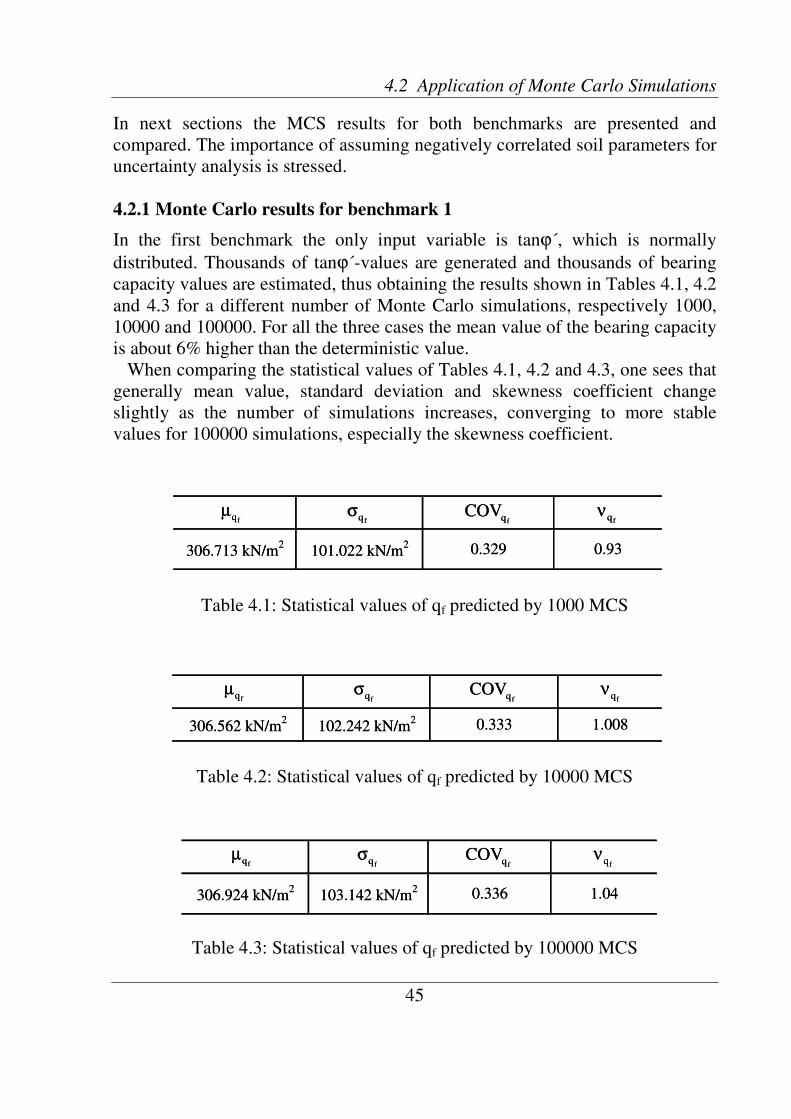
4.2 Application of Monte Carlo Simulations
45
fqµfqσ
fqCOVfqν
306.713 kN/m2
101.022 kN/m2 0.329 0.93
fqµfqσ
fqCOVfqν
306.713 kN/m2
101.022 kN/m2 0.329 0.93
fqµfqσ
fqCOVfqν
1.008306.562 kN/m2
102.242 kN/m2 0.333
fqµfqσ
fqCOVfqν
1.008306.562 kN/m2
102.242 kN/m2 0.333
fqµfqσ
fqCOVfqν
306.924 kN/m2
103.142 kN/m2 0.336 1.04
fqµfqσ
fqCOVfqν
306.924 kN/m2
103.142 kN/m2 0.336 1.04
In next sections the MCS results for both benchmarks are presented and
compared. The importance of assuming negatively correlated soil parameters for
uncertainty analysis is stressed.
4.2.1 Monte Carlo results for benchmark 1
In the first benchmark the only input variable is tanϕ´, which is normally
distributed. Thousands of tanϕ´-values are generated and thousands of bearing
capacity values are estimated, thus obtaining the results shown in Tables 4.1, 4.2
and 4.3 for a different number of Monte Carlo simulations, respectively 1000,
10000 and 100000. For all the three cases the mean value of the bearing capacity
is about 6% higher than the deterministic value.
When comparing the statistical values of Tables 4.1, 4.2 and 4.3, one sees that
generally mean value, standard deviation and skewness coefficient change
slightly as the number of simulations increases, converging to more stable
values for 100000 simulations, especially the skewness coefficient.
Table 4.1: Statistical values of qf predicted by 1000 MCS
Table 4.2: Statistical values of qf predicted by 10000 MCS
Table 4.3: Statistical values of qf predicted by 100000 MCS
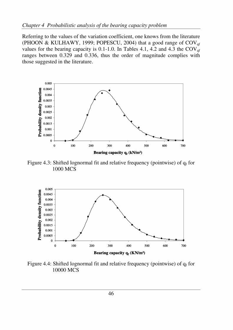
Chapter 4 Probabilistic analysis of the bearing capacity problem
46
Referring to the values of the variation coefficient, one knows from the literature
(PHOON & KULHAWY, 1999; POPESCU, 2004) that a good range of COVqf
values for the bearing capacity is 0.1-1.0. In Tables 4.1, 4.2 and 4.3 the COVqf
ranges between 0.329 and 0.336, thus the order of magnitude complies with
those suggested in the literature.
Figure 4.3: Shifted lognormal fit and relative frequency (pointwise) of qf for
1000 MCS
Figure 4.4: Shifted lognormal fit and relative frequency (pointwise) of qf for
10000 MCS
0
0.0005
0.001
0.0015
0.002
0.0025
0.003
0.0035
0.004
0.0045
0.005
0 100 200 300 400 500 600 700
Bearing capacity qf (kN/m²)
Pro
ba
bil
ity
den
sity
fun
ctio
n
0
0.0005
0.001
0.0015
0.002
0.0025
0.003
0.0035
0.004
0.0045
0.005
0 100 200 300 400 500 600 700
Bearing capacity qf (kN/m²)
Pro
ba
bil
ity
den
sity
fun
ctio
n
0
0.0005
0.001
0.0015
0.002
0.0025
0.003
0.0035
0.004
0.0045
0.005
0 100 200 300 400 500 600 700
Bearing capacity qf (KN/m²)
Pro
ba
bil
ity
den
sity
fun
ctio
n
0
0.0005
0.001
0.0015
0.002
0.0025
0.003
0.0035
0.004
0.0045
0.005
0 100 200 300 400 500 600 700
Bearing capacity qf (KN/m²)
Pro
ba
bil
ity
den
sity
fun
ctio
n
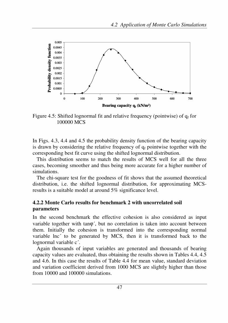
4.2 Application of Monte Carlo Simulations
47
Figure 4.5: Shifted lognormal fit and relative frequency (pointwise) of qf for
100000 MCS
In Figs. 4.3, 4.4 and 4.5 the probability density function of the bearing capacity
is drawn by considering the relative frequency of qf pointwise together with the
corresponding best fit curve using the shifted lognormal distribution.
This distribution seems to match the results of MCS well for all the three
cases, becoming smoother and thus being more accurate for a higher number of
simulations.
The chi-square test for the goodness of fit shows that the assumed theoretical
distribution, i.e. the shifted lognormal distribution, for approximating MCS-
results is a suitable model at around 5% significance level.
4.2.2 Monte Carlo results for benchmark 2 with uncorrelated soil
parameters
In the second benchmark the effective cohesion is also considered as input
variable together with tanϕ´, but no correlation is taken into account between
them. Initially the cohesion is transformed into the corresponding normal
variable lnc´ to be generated by MCS, then it is transformed back to the
lognormal variable c´.
Again thousands of input variables are generated and thousands of bearing
capacity values are evaluated, thus obtaining the results shown in Tables 4.4, 4.5
and 4.6. In this case the results of Table 4.4 for mean value, standard deviation
and variation coefficient derived from 1000 MCS are slightly higher than those
from 10000 and 100000 simulations.
0
0.0005
0.001
0.0015
0.002
0.0025
0.003
0.0035
0.004
0.0045
0.005
0 100 200 300 400 500 600 700
Bearing capacity qf (kN/m²)
Pro
ba
bil
ity
den
sity
fun
cti
on
0
0.0005
0.001
0.0015
0.002
0.0025
0.003
0.0035
0.004
0.0045
0.005
0 100 200 300 400 500 600 700
Bearing capacity qf (kN/m²)
Pro
ba
bil
ity
den
sity
fun
cti
on

Chapter 4 Probabilistic analysis of the bearing capacity problem
48
fqµfqσ
fqCOVfqν
1.387306.805 kN/m2 123.367 kN/m2 0.402
fqµfqσ
fqCOVfqν
1.387306.805 kN/m2 123.367 kN/m2 0.402
fqµfqσ
fqCOVfqν
310.807 kN/m2 130.135 kN/m2 0.419 1.255
fqµfqσ
fqCOVfqν
310.807 kN/m2 130.135 kN/m2 0.419 1.255
fqµfqσ
fqCOVfqν
306.451 kN/m2 122.807 kN/m2 0.401 1.393
fqµfqσ
fqCOVfqν
306.451 kN/m2 122.807 kN/m2 0.401 1.393
If the statistical values of Tables 4.1, 4.2 and 4.3 are compared to those of
Tables 4.4, 4.5 and 4.6, one sees that the mean value generally remains constant
and around 6% higher than the deterministic value, while the standard deviation
and the skewness coefficient increase. This is due to the consideration of the
cohesion as input variable, which introduces more uncertainty in the analysis.
The increase of the standard deviations results in higher COV values of the
bearing capacity than those of benchmark 1. However the values are similar to
those found in the literature.
In Figs. 4.6, 4.7 and 4.8 the relative frequency of the bearing capacity is again
plotted pointwise together with the probability density function by assuming a
shifted lognormal distribution as approximation.
Table 4.4: Statistical values of qf predicted by 1000 MCS with uncorrelated soil
variables
Table 4.5: Statistical values of qf predicted by 10000 MCS with uncorrelated
soil variables
Table 4.6: Statistical values of qf predicted by 100000 MCS with uncorrelated
soil variables
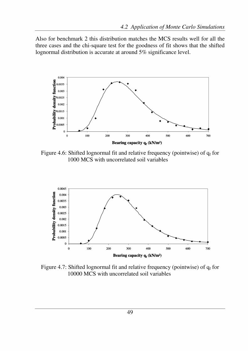
4.2 Application of Monte Carlo Simulations
49
Also for benchmark 2 this distribution matches the MCS results well for all the
three cases and the chi-square test for the goodness of fit shows that the shifted
lognormal distribution is accurate at around 5% significance level.
Figure 4.6: Shifted lognormal fit and relative frequency (pointwise) of qf for
1000 MCS with uncorrelated soil variables
Figure 4.7: Shifted lognormal fit and relative frequency (pointwise) of qf for
10000 MCS with uncorrelated soil variables
0
0.0005
0.001
0.0015
0.002
0.0025
0.003
0.0035
0.004
0 100 200 300 400 500 600 700
Bearing capacity qf (kN/m²)
Pro
ba
bil
ity
den
sity
fun
ctio
n
0
0.0005
0.001
0.0015
0.002
0.0025
0.003
0.0035
0.004
0 100 200 300 400 500 600 700
Bearing capacity qf (kN/m²)
Pro
ba
bil
ity
den
sity
fun
ctio
n
0
0.0005
0.001
0.0015
0.002
0.0025
0.003
0.0035
0.004
0.0045
0 100 200 300 400 500 600 700
Bearing capacity qf (kN/m²)
Pro
ba
bil
ity
den
sity
fun
ctio
n
0
0.0005
0.001
0.0015
0.002
0.0025
0.003
0.0035
0.004
0.0045
0 100 200 300 400 500 600 700
Bearing capacity qf (kN/m²)
Pro
ba
bil
ity
den
sity
fun
ctio
n
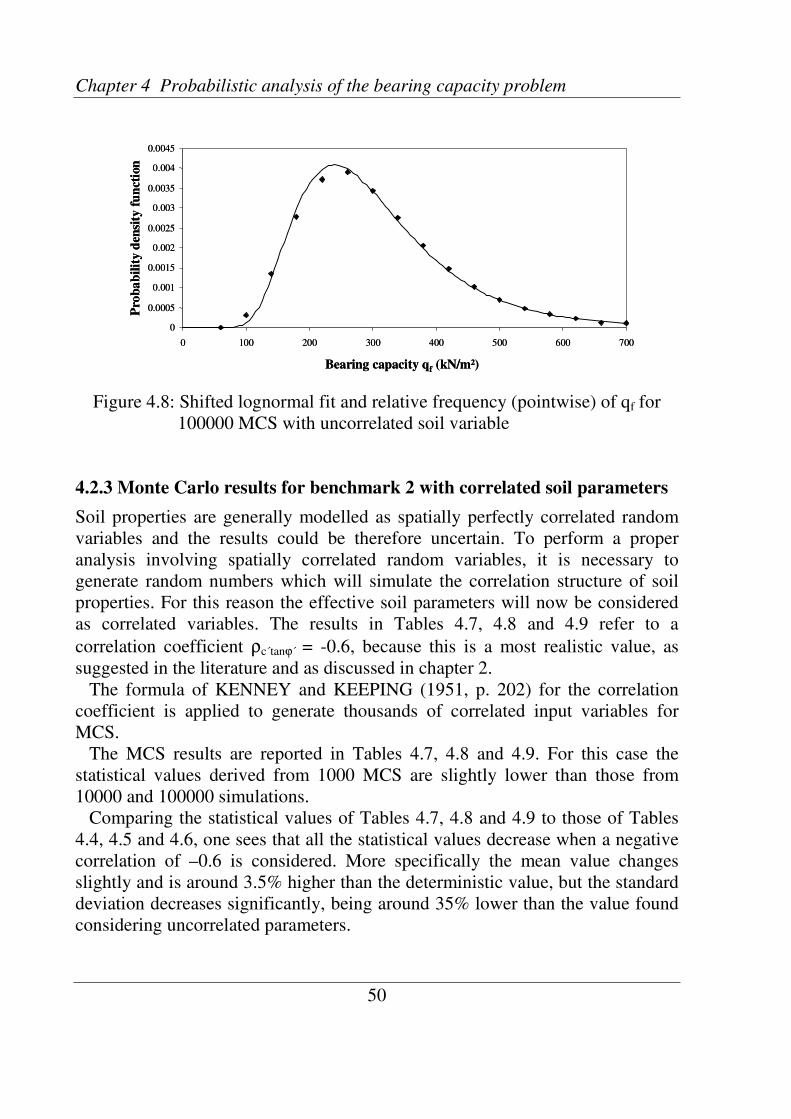
Chapter 4 Probabilistic analysis of the bearing capacity problem
50
Figure 4.8: Shifted lognormal fit and relative frequency (pointwise) of qf for
100000 MCS with uncorrelated soil variable
4.2.3 Monte Carlo results for benchmark 2 with correlated soil parameters
Soil properties are generally modelled as spatially perfectly correlated random
variables and the results could be therefore uncertain. To perform a proper
analysis involving spatially correlated random variables, it is necessary to
generate random numbers which will simulate the correlation structure of soil
properties. For this reason the effective soil parameters will now be considered
as correlated variables. The results in Tables 4.7, 4.8 and 4.9 refer to a
correlation coefficient ρc´tanϕ´ = -0.6, because this is a most realistic value, as
suggested in the literature and as discussed in chapter 2.
The formula of KENNEY and KEEPING (1951, p. 202) for the correlation
coefficient is applied to generate thousands of correlated input variables for
MCS.
The MCS results are reported in Tables 4.7, 4.8 and 4.9. For this case the
statistical values derived from 1000 MCS are slightly lower than those from
10000 and 100000 simulations.
Comparing the statistical values of Tables 4.7, 4.8 and 4.9 to those of Tables
4.4, 4.5 and 4.6, one sees that all the statistical values decrease when a negative
correlation of –0.6 is considered. More specifically the mean value changes
slightly and is around 3.5% higher than the deterministic value, but the standard
deviation decreases significantly, being around 35% lower than the value found
considering uncorrelated parameters.
0
0.0005
0.001
0.0015
0.002
0.0025
0.003
0.0035
0.004
0.0045
0 100 200 300 400 500 600 700
Bearing capacity qf (kN/m²)
Pro
ba
bil
ity
den
sity
fun
ctio
n
0
0.0005
0.001
0.0015
0.002
0.0025
0.003
0.0035
0.004
0.0045
0 100 200 300 400 500 600 700
Bearing capacity qf (kN/m²)
Pro
ba
bil
ity
den
sity
fun
ctio
n

4.2 Application of Monte Carlo Simulations
51
fqµfqσ
fqCOVfqν
297.848 kN/m2 73.372 kN/m2 0.246 0.911
fqµfqσ
fqCOVfqν
297.848 kN/m2 73.372 kN/m2 0.246 0.911
fqµfqσ
fqCOVfqν
294.288 kN/m2 72.011 kN/m2 0.245 1.115
fqµfqσ
fqCOVfqν
294.288 kN/m2 72.011 kN/m2 0.245 1.115
fqµfqσ
fqCOVfqν
297.327 kN/m2 73.795 kN/m2 0.248 0.952
fqµfqσ
fqCOVfqν
297.327 kN/m2 73.795 kN/m2 0.248 0.952
As a consequence the skewness and the variation coefficients also decrease.
Thus the variability of the bearing capacity and the uncertainty in the analysis
decrease considerably.
The frequency diagrams of Figs. 4.9, 4.10, 4.11 and the shifted lognormal fits
show that these plots become narrower and the corresponding peak values
consequently higher than those of the case with uncorrelated soil parameters.
This difference can be seen better in Fig. 4.12, where the probability density
function of qf from 10000 MCS for soil parameters having no correlation and a
value of ρc´tanϕ´ = -0.6 are plotted together. For uncorrelated variables the density
function is wider and the peak value is 0.0043, whereas for negatively correlated
variables the curve is narrower reaching a peak value of 0.0062.
Table 4.7: Statistical values of qf predicted by 1000 MCS with negatively
correlated variables
Table 4.8: Statistical values of qf predicted by 10000 MCS with negatively
correlated variables
Table 4.9: Statistical values of qf predicted by 100000 MCS with negatively
correlated variables

Chapter 4 Probabilistic analysis of the bearing capacity problem
52
It is also clear that the variability of the bearing capacity considering correlated
soil parameters decreases, starting from a value of around 120 kN/m2 for non-
zero probabilities compared to a value of around 80 kN/m2, for the case with
uncorrelated variables.
Figure 4.9: Shifted lognormal fit and relative frequency (pointwise) of qf for
1000 MCS with negatively correlated variables
Figure 4.10: Shifted lognormal fit and relative frequency (pointwise) of qf for
10000 MCS with negatively correlated variables
0
0.001
0.002
0.003
0.004
0.005
0.006
0.007
0 100 200 300 400 500 600 700
Bearing capacity qf (kN/m²)
Pro
ba
bil
ity
den
sity
fun
ctio
n
0
0.001
0.002
0.003
0.004
0.005
0.006
0.007
0 100 200 300 400 500 600 700
Bearing capacity qf (kN/m²)
Pro
ba
bil
ity
den
sity
fun
ctio
n
0
0.001
0.002
0.003
0.004
0.005
0.006
0.007
0 100 200 300 400 500 600 700
Bearing capacity qf (kN/m²)
Pro
bab
ilit
yd
ensi
tyfu
nct
ion
0
0.001
0.002
0.003
0.004
0.005
0.006
0.007
0 100 200 300 400 500 600 700
Bearing capacity qf (kN/m²)
Pro
bab
ilit
yd
ensi
tyfu
nct
ion

4.2 Application of Monte Carlo Simulations
53
0
0.001
0.002
0.003
0.004
0.005
0.006
0.007
0 40 80 120 160 200 240 280 320 360 400 440 480 520 560 600
Bearing capacity qf(kN/m²)
Pro
bab
ilit
yd
en
sity
fun
cti
on
0tan =ρϕ′′c
6.0tan −=ρϕ′′c
0
0.001
0.002
0.003
0.004
0.005
0.006
0.007
0 40 80 120 160 200 240 280 320 360 400 440 480 520 560 600
Bearing capacity qf(kN/m²)
Pro
bab
ilit
yd
en
sity
fun
cti
on
0
0.001
0.002
0.003
0.004
0.005
0.006
0
0.001
0.002
0.003
0.004
0.005
0.006
0.007
0 40 80 120 160 200 240 280 320 360 400 440 480 520 560 600
Bearing capacity qf(kN/m²)
Pro
bab
ilit
yd
en
sity
fun
cti
on
0tan =ρϕ′′c
6.0tan −=ρϕ′′c
Figure 4.11: Shifted lognormal fit and relative frequency (pointwise) of qf for
100000 MCS with negatively correlated variables
Figure 4.12: Comparison of shifted lognormal fits of qf from 10000 MCS for
uncorrelated and negatively correlated soil variables
In Table 4.10 the statistical values of the bearing capacity are listed for different
correlation coefficients from –0.9 to 0.0. Because of some limitations in the
KENNEY and KEEPING’s formula, the value ρc´tanϕ´ = -1.0 can not be taken
into account.
By decreasing the correlation coefficient, the mean value changes slightly.
Whereas the standard deviation decreases significantly, from around 123.4
kN/m2 when there is no correlation between soil parameters down to around
50.3 kN/m2, when ρc´tanϕ´ = -0.9.
0
0.001
0.002
0.003
0.004
0.005
0.006
0.007
0 100 200 300 400 500 600 700
Bearing capacity qf (kN/m²)
Pro
ba
bil
ity
den
sity
fun
ctio
n
0
0.001
0.002
0.003
0.004
0.005
0.006
0.007
0 100 200 300 400 500 600 700
Bearing capacity qf (kN/m²)
Pro
ba
bil
ity
den
sity
fun
ctio
n

Chapter 4 Probabilistic analysis of the bearing capacity problem
54
)/( 2mkNfqµ )/( 2mkN
fqσϕ′′ρ tancfqν
-0.9 294.635 50.321 2.244
-0.8 295.616 57.661 1.462
-0.7 296.734 65.774 1.057
-0.6 297.848 73.372 0.911
-0.5 299.071 81.274 0.877
-0.4 300.305 88.902 0.932
-0.3 301.448 95.729 1.004
-0.2 302.709 103.054 1.100
-0.1 303.986 110.295 1.206
0.0 306.805 123.367 1.387
)/( 2mkNfqµ )/( 2mkN
fqσϕ′′ρ tancfqν
-0.9 294.635 50.321 2.244
-0.8 295.616 57.661 1.462
-0.7 296.734 65.774 1.057
-0.6 297.848 73.372 0.911
-0.5 299.071 81.274 0.877
-0.4 300.305 88.902 0.932
-0.3 301.448 95.729 1.004
-0.2 302.709 103.054 1.100
-0.1 303.986 110.295 1.206
0.0 306.805 123.367 1.387
The skewness coefficient has a strange behaviour. In fact, when the correlation
decreases from ρc´tanϕ´ = 0 down to the value ρc´tanϕ´ = -0.5, the skewness
coefficient decreases too. If one proceed to reduce the correlation down to ρc´tanϕ´
= -0.9, then the skewness coefficient increases, reaching a maximum value of
2.244.
Fig. 4.13 shows the influence of the correlation coefficient variation on the
shape of the shifted lognormal fit of the bearing capacity. As already pointed out
in Fig. 4.12, the curves become narrower for lower correlation coefficients, thus
decreasing the variability of the bearing capacity and increasing the peak of the
fit. It is also clear how the skewness coefficient changes the shape of the curves
from the least skewed curve for ρc´tanϕ´ = -0.5 to the most skewed one for ρc´tanϕ´ =
-0.9.
Recapitulating all these observations, it is then possible to conclude that the
choice of a negative correlation for the soil parameters is reasonable, because
the uncertainty in the problem decreases considerably.
Notwithstanding the accuracy of MCS results, this method is too time
consuming for practical computations, therefore alternative methods need to be
considered. In next sections the FOSM and SOSM methods are applied to the
same bearing capacity benchmark.
Table 4.10: Influence of ρc´tanϕ´ on the statistical values of qf from MCS

4.3 Application of the FOSM method
55
0
0.002
0.004
0.006
0.008
0.01
0.012
0.014
0 40 80 120 160 200 240 280 320 360 400 440 480 520 560 600
Bearing capacity qf (kN/m²)
Prob
ab
ilit
yd
ensi
tyfu
ncti
on
0 -0.1 -0.2 -0.3 -0.4 -0.5 -0.6 -0.7 -0.8 -0.9
0tanc =ρϕ′′
5.0tanc −=ρϕ′′
9.0tanc −=ρϕ′′
0
0.002
0.004
0.006
0.008
0.01
0.012
0.014
0 40 80 120 160 200 240 280 320 360 400 440 480 520 560 600
Bearing capacity qf (kN/m²)
Prob
ab
ilit
yd
ensi
tyfu
ncti
on
0 -0.1 -0.2 -0.3 -0.4 -0.5 -0.6 -0.7 -0.8 -0.9
0
0.002
0.004
0.006
0.008
0.01
0.012
0.014
0 40 80 120 160 200 240 280 320 360 400 440 480 520 560 600
Bearing capacity qf (kN/m²)
Prob
ab
ilit
yd
ensi
tyfu
ncti
on
0 -0.1 -0.2 -0.3 -0.4 -0.5 -0.6 -0.7 -0.8 -0.9
0tanc =ρϕ′′
5.0tanc −=ρϕ′′
9.0tanc −=ρϕ′′
0tanc =ρϕ′′
5.0tanc −=ρϕ′′
9.0tanc −=ρϕ′′
Figure 4.13: Influence of the correlation coefficient variation on the shifted
lognormal fit of qf for 10000 MCS
4.3 Application of the FOSM method
It was highlighted in chapter 2 that the simplest alternative to MCS is the FOSM
method, which produces a linearisation around the mean value of the input soil
variables. The next sections will show the results of FOSM application to the
benchmarks already considered.
4.3.1 FOSM results for benchmark 1
Considering Terzaghi´s bearing capacity formula (A.4) in appendix A as a
function of tanϕ´, the Taylor’s series expansion for the bearing capacity about
the mean value µtanϕ´ truncated after the first order terms is given by
( ) ( )ϕ′∂
∂⋅µ−ϕ′+µ≈
ϕ′ϕ′
tan
qtanqq f
tantanff (4.2)
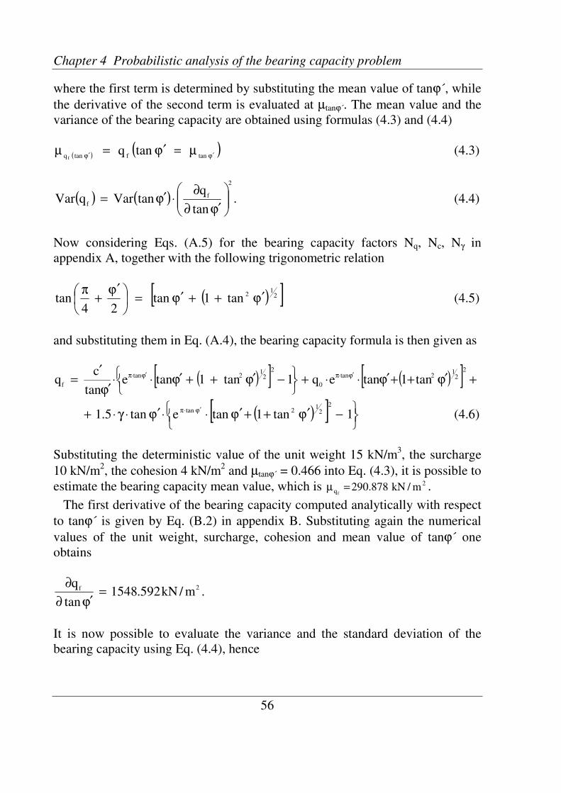
Chapter 4 Probabilistic analysis of the bearing capacity problem
56
where the first term is determined by substituting the mean value of tanϕ´, while
the derivative of the second term is evaluated at µtanϕ´. The mean value and the
variance of the bearing capacity are obtained using formulas (4.3) and (4.4)
( )( )
ϕ′ϕ′µ=ϕ′=µ
tanftanqtanq
f (4.3)
( ) ( ) .tan
qtanVarqVar
2
f
f
ϕ′∂
∂⋅ϕ′= (4.4)
Now considering Eqs. (A.5) for the bearing capacity factors Nq, Nc, Nγ in
appendix A, together with the following trigonometric relation
( )[ ]21
2tan1tan
24tan ϕ′++ϕ′=
ϕ′+
π (4.5)
and substituting them in Eq. (A.4), the bearing capacity formula is then given as
( )[ ] ( )[ ] +ϕ′++ϕ′⋅⋅+
−ϕ′++ϕ′⋅⋅ϕ′
′=
ϕ′⋅πϕ′⋅π2
21
2tan
0
22
12tan
ftan1taneq1tan1tane
tan
cq
( )[ ]
−ϕ′++ϕ′⋅⋅ϕ′⋅γ⋅+ϕ′⋅π 1tan1tanetan5.1
22
12tan (4.6)
Substituting the deterministic value of the unit weight 15 kN/m3, the surcharge
10 kN/m2, the cohesion 4 kN/m
2 and µtanϕ´ = 0.466 into Eq. (4.3), it is possible to
estimate the bearing capacity mean value, which is 2/878.290 mkNfq =µ .
The first derivative of the bearing capacity computed analytically with respect
to tanϕ´ is given by Eq. (B.2) in appendix B. Substituting again the numerical
values of the unit weight, surcharge, cohesion and mean value of tanϕ´ one
obtains
2f m/kN592.1548tan
q=
ϕ′∂
∂.
It is now possible to evaluate the variance and the standard deviation of the
bearing capacity using Eq. (4.4), hence
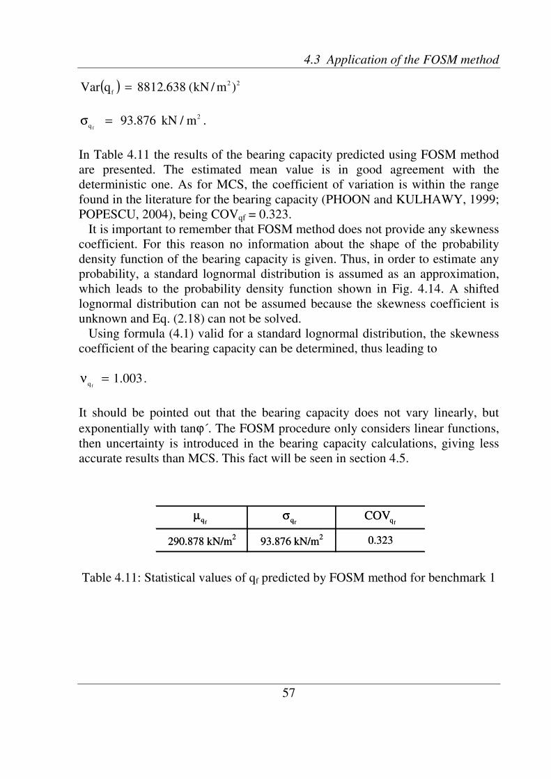
4.3 Application of the FOSM method
57
fqµfqσ
fqCOV
290.878 kN/m2
93.876 kN/m2 0.323
fqµfqσ
fqCOV
290.878 kN/m2
93.876 kN/m2 0.323
( ) 22
f)m/kN(638.8812qVar =
.m/kN876.93 2
q f=σ
In Table 4.11 the results of the bearing capacity predicted using FOSM method
are presented. The estimated mean value is in good agreement with the
deterministic one. As for MCS, the coefficient of variation is within the range
found in the literature for the bearing capacity (PHOON and KULHAWY, 1999;
POPESCU, 2004), being COVqf = 0.323.
It is important to remember that FOSM method does not provide any skewness
coefficient. For this reason no information about the shape of the probability
density function of the bearing capacity is given. Thus, in order to estimate any
probability, a standard lognormal distribution is assumed as an approximation,
which leads to the probability density function shown in Fig. 4.14. A shifted
lognormal distribution can not be assumed because the skewness coefficient is
unknown and Eq. (2.18) can not be solved.
Using formula (4.1) valid for a standard lognormal distribution, the skewness
coefficient of the bearing capacity can be determined, thus leading to
003.1fq
=ν .
It should be pointed out that the bearing capacity does not vary linearly, but
exponentially with tanϕ´. The FOSM procedure only considers linear functions,
then uncertainty is introduced in the bearing capacity calculations, giving less
accurate results than MCS. This fact will be seen in section 4.5.
Table 4.11: Statistical values of qf predicted by FOSM method for benchmark 1
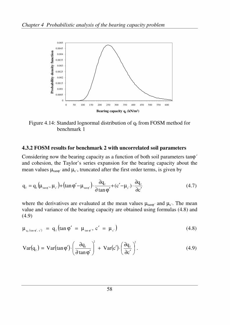
Chapter 4 Probabilistic analysis of the bearing capacity problem
58
Figure 4.14: Standard lognormal distribution of qf from FOSM method for
benchmark 1
4.3.2 FOSM results for benchmark 2 with uncorrelated soil parameters
Considering now the bearing capacity as a function of both soil parameters tanϕ´
and cohesion, the Taylor’s series expansion for the bearing capacity about the
mean values µtanϕ´ and µc´, truncated after the first order terms, is given by
( ) ( )c
q)c(
tan
qtan,qq f
c
f
tanctanff′∂
∂⋅µ−′+
ϕ′∂
∂⋅µ−ϕ′+µµ=
′ϕ′′ϕ′ (4.7)
where the derivatives are evaluated at the mean values µtanϕ´ and µc´. The mean
value and variance of the bearing capacity are obtained using formulas (4.8) and
(4.9)
( )( )
ctanfc,tanqc,tanq
f ′ϕ′′ϕ′µ=′µ=ϕ′=µ (4.8)
( ) ( ) ( ) .c
qcVar
tan
qtanVarqVar
2
f
2
f
f
′∂
∂⋅′+
ϕ′∂
∂⋅ϕ′= (4.9)
0
0.0005
0.001
0.0015
0.002
0.0025
0.003
0.0035
0.004
0.0045
0.005
0 50 100 150 200 250 300 350 400 450 500 550 600
Bearing capacity qf (kN/m²)
Pro
bab
ilit
yd
en
sity
fun
cti
on
0
0.0005
0.001
0.0015
0.002
0.0025
0.003
0.0035
0.004
0.0045
0.005
0 50 100 150 200 250 300 350 400 450 500 550 600
Bearing capacity qf (kN/m²)
Pro
bab
ilit
yd
en
sity
fun
cti
on
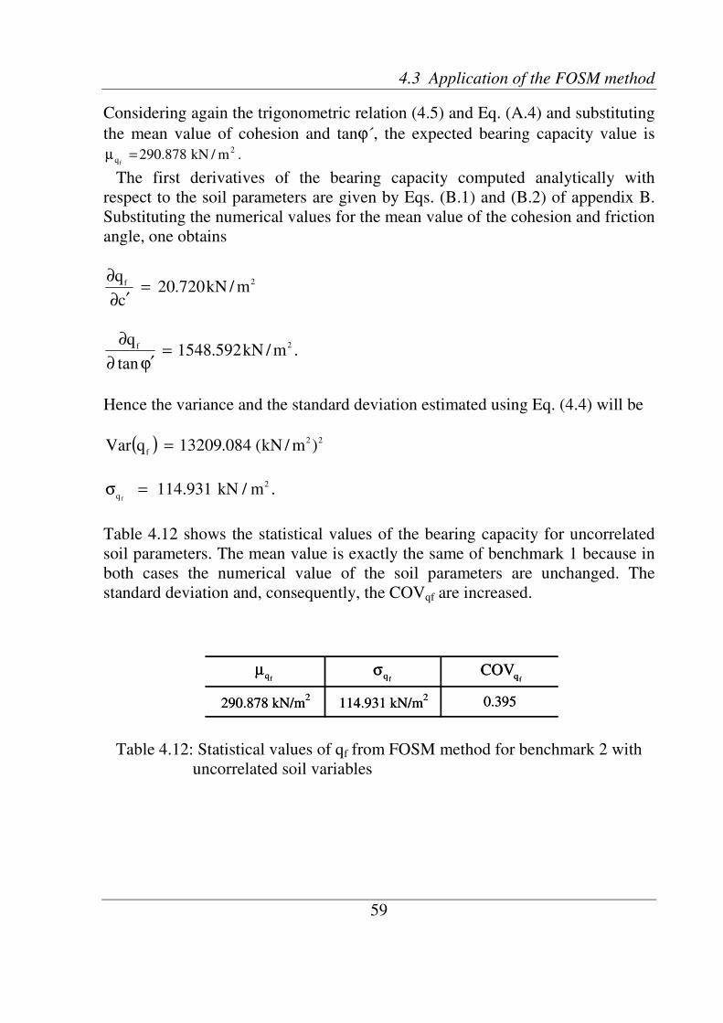
4.3 Application of the FOSM method
59
290.878 kN/m2
114.931 kN/m2 0.395
fqµfqσ
fqCOV
290.878 kN/m2
114.931 kN/m2 0.395
fqµfqσ
fqCOV
Considering again the trigonometric relation (4.5) and Eq. (A.4) and substituting
the mean value of cohesion and tanϕ´, the expected bearing capacity value is
./878.290 2mkNfq =µ
The first derivatives of the bearing capacity computed analytically with
respect to the soil parameters are given by Eqs. (B.1) and (B.2) of appendix B.
Substituting the numerical values for the mean value of the cohesion and friction
angle, one obtains
2f m/kN720.20c
q=
′∂
∂
.m/kN592.1548tan
q 2f=
ϕ′∂
∂
Hence the variance and the standard deviation estimated using Eq. (4.4) will be
( ) 22
f)m/kN(084.13209qVar =
2
qm/kN931.114
f=σ .
Table 4.12 shows the statistical values of the bearing capacity for uncorrelated
soil parameters. The mean value is exactly the same of benchmark 1 because in
both cases the numerical value of the soil parameters are unchanged. The
standard deviation and, consequently, the COVqf are increased.
Table 4.12: Statistical values of qf from FOSM method for benchmark 2 with
uncorrelated soil variables
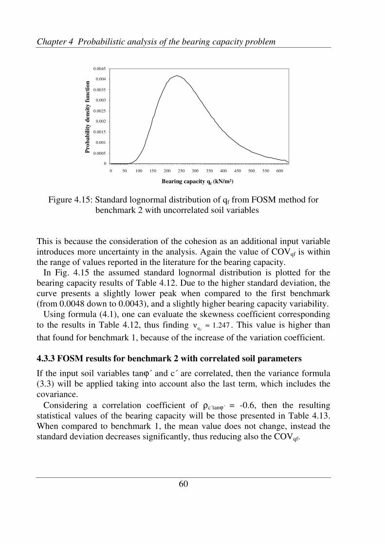
Chapter 4 Probabilistic analysis of the bearing capacity problem
60
Figure 4.15: Standard lognormal distribution of qf from FOSM method for
benchmark 2 with uncorrelated soil variables
This is because the consideration of the cohesion as an additional input variable
introduces more uncertainty in the analysis. Again the value of COVqf is within
the range of values reported in the literature for the bearing capacity.
In Fig. 4.15 the assumed standard lognormal distribution is plotted for the
bearing capacity results of Table 4.12. Due to the higher standard deviation, the
curve presents a slightly lower peak when compared to the first benchmark
(from 0.0048 down to 0.0043), and a slightly higher bearing capacity variability.
Using formula (4.1), one can evaluate the skewness coefficient corresponding
to the results in Table 4.12, thus finding 247.1≈νfq . This value is higher than
that found for benchmark 1, because of the increase of the variation coefficient.
4.3.3 FOSM results for benchmark 2 with correlated soil parameters
If the input soil variables tanϕ´ and c´ are correlated, then the variance formula
(3.3) will be applied taking into account also the last term, which includes the
covariance.
Considering a correlation coefficient of ρc´tanϕ´ = -0.6, then the resulting
statistical values of the bearing capacity will be those presented in Table 4.13.
When compared to benchmark 1, the mean value does not change, instead the
standard deviation decreases significantly, thus reducing also the COVqf.
0
0.0005
0.001
0.0015
0.002
0.0025
0.003
0.0035
0.004
0.0045
0 50 100 150 200 250 300 350 400 450 500 550 600
Bearing capacity qf (kN/m²)
Pro
bab
ilit
yd
en
sity
fun
cti
on
0
0.0005
0.001
0.0015
0.002
0.0025
0.003
0.0035
0.004
0.0045
0 50 100 150 200 250 300 350 400 450 500 550 600
Bearing capacity qf (kN/m²)
Pro
bab
ilit
yd
en
sity
fun
cti
on
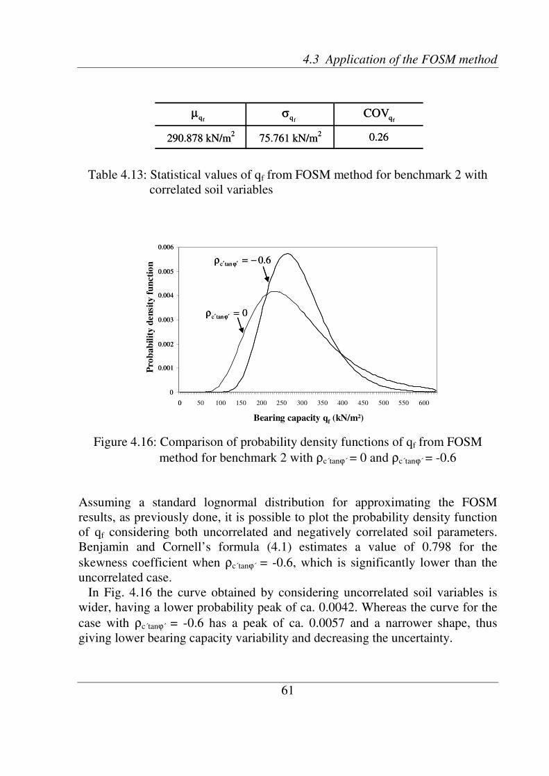
4.3 Application of the FOSM method
61
290.878 kN/m2
75.761 kN/m2 0.26
fqµfqσ
fqCOV
290.878 kN/m2
75.761 kN/m2 0.26
fqµfqσ
fqCOV
0
0.001
0.002
0.003
0.004
0.005
0.006
0 50 100 150 200 250 300 350 400 450 500 550 600
Bearing capacity qf(kN/m²)
Pro
bab
ilit
yd
en
sity
fun
cti
on
0tan =ρϕ′′c
6.0tan −=ρϕ′′c
0
0.001
0.002
0.003
0.004
0.005
0.006
0 50 100 150 200 250 300 350 400 450 500 550 600
Bearing capacity qf(kN/m²)
Pro
bab
ilit
yd
en
sity
fun
cti
on
0
0.001
0.002
0.003
0.004
0.005
0.006
0
0
0.001
0.002
0.003
0.004
0.005
0.006
0 50 100 150 200 250 300 350 400 450 500 550 600
Bearing capacity qf(kN/m²)
Pro
bab
ilit
yd
en
sity
fun
cti
on
0tan =ρϕ′′c
6.0tan −=ρϕ′′c
0tan =ρϕ′′c
6.0tan −=ρϕ′′c
Table 4.13: Statistical values of qf from FOSM method for benchmark 2 with
correlated soil variables
Figure 4.16: Comparison of probability density functions of qf from FOSM
method for benchmark 2 with ρc´tanϕ´ = 0 and ρc´tanϕ´ = -0.6
Assuming a standard lognormal distribution for approximating the FOSM
results, as previously done, it is possible to plot the probability density function
of qf considering both uncorrelated and negatively correlated soil parameters.
Benjamin and Cornell’s formula (4.1) estimates a value of 0.798 for the
skewness coefficient when ρc´tanϕ´ = -0.6, which is significantly lower than the
uncorrelated case.
In Fig. 4.16 the curve obtained by considering uncorrelated soil variables is
wider, having a lower probability peak of ca. 0.0042. Whereas the curve for the
case with ρc´tanϕ´ = -0.6 has a peak of ca. 0.0057 and a narrower shape, thus
giving lower bearing capacity variability and decreasing the uncertainty.

Chapter 4 Probabilistic analysis of the bearing capacity problem
62
)m/kN(2
qfσϕ′′ρ tanc
-1.0 27.570
-0.9 44.777
-0.8 57.008
-0.7 67.043
-0.6 75.761
-0.5 83.574
-0.4 90.717
-0.3 97.336
-0.2 103.534
-0.1 109.381
0.0 114.931
)m/kN(2
qfσϕ′′ρ tanc
-1.0 27.570
-0.9 44.777
-0.8 57.008
-0.7 67.043
-0.6 75.761
-0.5 83.574
-0.4 90.717
-0.3 97.336
-0.2 103.534
-0.1 109.381
0.0 114.931
Varying the correlation coefficient from 0 to –1.0, the standard deviation of qf
decreases down to around 76% for ρc´tanϕ´ = -1.0, as shown in Table 4.14, while
the mean value is always constant and equal to 290.878 kN/m².
If the standard lognormal distribution would be assumed to draw the
probability density curves of the bearing capacity results of Table 4.14, then the
same conclusions of Fig. 4.13 about the shape of the curves and the variability
of the bearing capacity with the correlation between the input soil parameters
would come out.
Summarizing all these observations it seems to be very important for
probabilistic analysis to include a negative correlation between cohesion and
friction angle in order to have less uncertainty in the final results.
Table 4.14: Influence of ρc´tanϕ´ on the standard deviation of qf from FOSM
method for benchmark 2 with uncorrelated and negatively
correlated soil variables
4.4 Application of the SOSM method
FOSM method can be slightly extended for a better prediction of the bearing
capacity mean value through the SOSM method. Results of this approach will be
illustrated in the next section and compared to those of Monte Carlo and FOSM
methods.

4.4 Application of the SOSM method
63
303.851 kN/m2
93.876 kN/m2 0.309
fqµfqσ
fqCOV
303.851 kN/m2
93.876 kN/m2 0.309
fqµfqσ
fqCOV
4.4.1 SOSM results for benchmark 1
Second order terms of Taylor’s series expansion of the bearing capacity will be
now added to Eq. (4.3). In this way it is possible to refine the estimate of the
bearing capacity mean value, leading to
( ) ( ) ( )ϕ′∂
∂⋅ϕ′⋅+
ϕ′∂
∂⋅µ−ϕ′+µ=µ
ϕ′ϕ′ 2
f
2
f
tantanfqtan
qtanVar
2
1
tan
qtanq
f (4.10)
where the derivatives, given by Eqs. (B.1) and (B.4) of appendix B, are
evaluated at µtanϕ´. Substituting the numerical values for unit weight, surcharge,
cohesion and the mean value of tanϕ´, the first derivative of the bearing capacity
is the same as for FOSM method in section 4.3.1, while the second derivative is
given by
.m/kN685.7060tan
q 2
2
f
2
=ϕ′∂
∂
Then the bearing capacity mean value, given by Eq. (4.10), will be 2/851.303 mkN
fq =µ .
The statistical values of the bearing capacity derived from SOSM application
are shown in Table 4.15. The mean value is around 5% higher than the
deterministic value. Comparing these results to those of Table 4.11 for FOSM
method, one sees that the second order terms have increased the mean value of
the bearing capacity µqf and thus reduced the COVqf value, while the standard
deviation remains constant.
Assuming a standard lognormal distribution, the probability density function
of the bearing capacity is plotted in Fig. 4.17. In this case the skewness
coefficient, evaluated with formula (4.1), will be 956.0≈νfq , which is slightly
lower than the value found with FOSM method.
Table 4.15: Statistical values of qf from SOSM method for benchmark 1
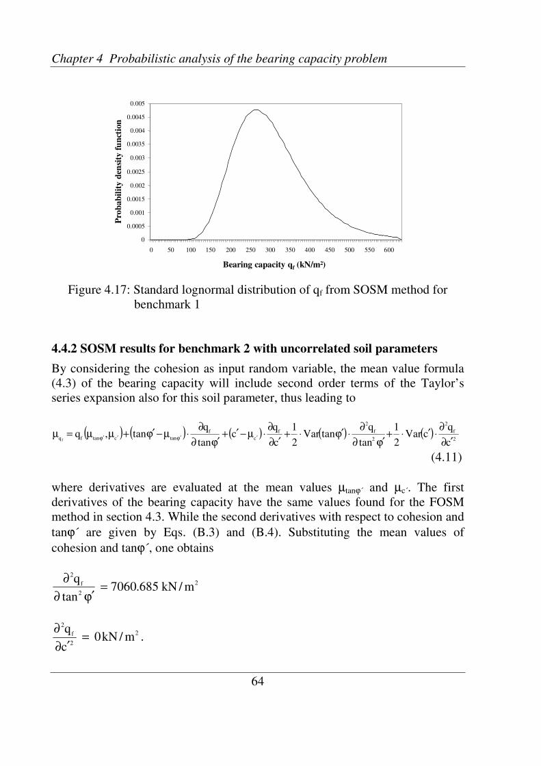
Chapter 4 Probabilistic analysis of the bearing capacity problem
64
Figure 4.17: Standard lognormal distribution of qf from SOSM method for
benchmark 1
4.4.2 SOSM results for benchmark 2 with uncorrelated soil parameters
By considering the cohesion as input random variable, the mean value formula
(4.3) of the bearing capacity will include second order terms of the Taylor’s
series expansion also for this soil parameter, thus leading to
( ) ( ) ( ) ( ) ( )2
f
2
2
f
2
f
c
f
tanctanfqc
qcVar
2
1
tan
qtanVar
2
1
c
qc
tan
qtan,q
f ′∂
∂⋅′⋅+
ϕ′∂
∂⋅ϕ′⋅+
′∂
∂⋅µ−′+
ϕ′∂
∂⋅µ−ϕ′+µµ=µ
′ϕ′′ϕ′
(4.11)
where derivatives are evaluated at the mean values µtanϕ´ and µc´. The first
derivatives of the bearing capacity have the same values found for the FOSM
method in section 4.3. While the second derivatives with respect to cohesion and
tanϕ´ are given by Eqs. (B.3) and (B.4). Substituting the mean values of
cohesion and tanϕ´, one obtains
2
2
f
2
m/kN685.7060tan
q=
ϕ′∂
∂
2
2
f
2
m/kN0c
q=
′∂
∂.
0
0.0005
0.001
0.0015
0.002
0.0025
0.003
0.0035
0.004
0.0045
0.005
0 50 100 150 200 250 300 350 400 450 500 550 600
Bearing capacity qf (kN/m²)
Pro
ba
bil
ity
den
sity
fun
ctio
n
0
0.0005
0.001
0.0015
0.002
0.0025
0.003
0.0035
0.004
0.0045
0.005
0 50 100 150 200 250 300 350 400 450 500 550 600
Bearing capacity qf (kN/m²)
Pro
ba
bil
ity
den
sity
fun
ctio
n

4.4 Application of the SOSM method
65
303.851 kN/m2
114.931 kN/m2 0.378
fqµfqσ
fqCOV
303.851 kN/m2
114.931 kN/m2 0.378
fqµfqσ
fqCOV
Then the bearing capacity mean value, given by Eq. (4.11), will be 2
qm/kN851.303
f=µ . The corresponding statistical estimates of the bearing
capacity are shown in Table 4.16.
Comparing these results to those of Table 4.12, one notes that the second order
terms have increased the mean value µqf, thus reducing COVqf value, while the
standard deviation is still the same. These results are shown in Fig. 4.18
assuming a standard lognormal distribution as approximation. Using Benjamin
and Cornell’s formula (4.1), the skewness coefficient value is 188.1fq
≈ν ,
which is slightly lower than the value found by FOSM method for uncorrelated
input variables.
Table 4.16: Statistical values of qf from SOSM method for benchmark 2 with
uncorrelated soil variables
Figure 4.18: Standard lognormal distribution of qf from SOSM method for
benchmark 2 with uncorrelated soil variables
0
0.0005
0.001
0.0015
0.002
0.0025
0.003
0.0035
0.004
0.0045
0 50 100 150 200 250 300 350 400 450 500 550 600
Bearing capacity qf (kN/m²)
Pro
ba
bil
ity
den
sity
fun
ctio
n
0
0.0005
0.001
0.0015
0.002
0.0025
0.003
0.0035
0.004
0.0045
0 50 100 150 200 250 300 350 400 450 500 550 600
Bearing capacity qf (kN/m²)
Pro
ba
bil
ity
den
sity
fun
ctio
n
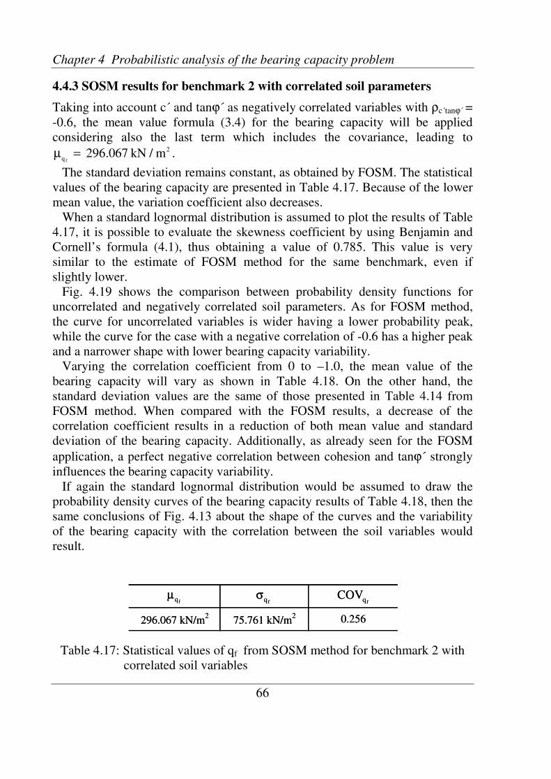
Chapter 4 Probabilistic analysis of the bearing capacity problem
66
296.067 kN/m2
75.761 kN/m2 0.256
fqµfqσ
fqCOV
296.067 kN/m2
75.761 kN/m2 0.256
fqµfqσ
fqCOV
4.4.3 SOSM results for benchmark 2 with correlated soil parameters
Taking into account c´ and tanϕ´ as negatively correlated variables with ρc´tanϕ´ =
-0.6, the mean value formula (3.4) for the bearing capacity will be applied
considering also the last term which includes the covariance, leading to 2
qm/kN067.296
f=µ .
The standard deviation remains constant, as obtained by FOSM. The statistical
values of the bearing capacity are presented in Table 4.17. Because of the lower
mean value, the variation coefficient also decreases.
When a standard lognormal distribution is assumed to plot the results of Table
4.17, it is possible to evaluate the skewness coefficient by using Benjamin and
Cornell’s formula (4.1), thus obtaining a value of 0.785. This value is very
similar to the estimate of FOSM method for the same benchmark, even if
slightly lower.
Fig. 4.19 shows the comparison between probability density functions for
uncorrelated and negatively correlated soil parameters. As for FOSM method,
the curve for uncorrelated variables is wider having a lower probability peak,
while the curve for the case with a negative correlation of -0.6 has a higher peak
and a narrower shape with lower bearing capacity variability.
Varying the correlation coefficient from 0 to –1.0, the mean value of the
bearing capacity will vary as shown in Table 4.18. On the other hand, the
standard deviation values are the same of those presented in Table 4.14 from
FOSM method. When compared with the FOSM results, a decrease of the
correlation coefficient results in a reduction of both mean value and standard
deviation of the bearing capacity. Additionally, as already seen for the FOSM
application, a perfect negative correlation between cohesion and tanϕ´ strongly
influences the bearing capacity variability.
If again the standard lognormal distribution would be assumed to draw the
probability density curves of the bearing capacity results of Table 4.18, then the
same conclusions of Fig. 4.13 about the shape of the curves and the variability
of the bearing capacity with the correlation between the soil variables would
result.
Table 4.17: Statistical values of qf from SOSM method for benchmark 2 with
correlated soil variables

4.4 Application of the SOSM method
67
)/(2
mkNfqµ )/(
2mkN
fqσϕ′′ρ tanc
-1.0 290.878 27.570
-0.9 292.175 44.777
-0.8 293.472 57.008
-0.7 294.770 67.043
-0.6 296.067 75.761
-0.5 297.364 83.574
-0.4 298.662 90.717
-0.3 299.959 97.336
-0.2 301.257 103.534
-0.1 302.554 109.381
0.0 303.851 114.931
)/(2
mkNfqµ )/(
2mkN
fqσϕ′′ρ tanc
-1.0 290.878 27.570
-0.9 292.175 44.777
-0.8 293.472 57.008
-0.7 294.770 67.043
-0.6 296.067 75.761
-0.5 297.364 83.574
-0.4 298.662 90.717
-0.3 299.959 97.336
-0.2 301.257 103.534
-0.1 302.554 109.381
0.0 303.851 114.931
0
0.001
0.002
0.003
0.004
0.005
0.006
0 50 100 150 200 250 300 350 400 450 500 550 600
Bearing capacity qf(kN/m²)
Pro
bab
ilit
yd
en
sity
fun
cti
on
0tan =ρϕ′′c
6.0tan −=ρϕ′′c
0
0.001
0.002
0.003
0.004
0.005
0.006
0 50 100 150 200 250 300 350 400 450 500 550 600
Bearing capacity qf(kN/m²)
Pro
bab
ilit
yd
en
sity
fun
cti
on
0
0.001
0.002
0.003
0.004
0.005
0.006
0
0
0.001
0.002
0.003
0.004
0.005
0.006
0 50 100 150 200 250 300 350 400 450 500 550 600
Bearing capacity qf(kN/m²)
Pro
bab
ilit
yd
en
sity
fun
cti
on
0tan =ρϕ′′c
6.0tan −=ρϕ′′c
Summing up all these observations, it would seem that SOSM method can refine
the estimate of the bearing capacity mean value. However results show that the
improvement is small and hardly worthwhile for the proposed benchmarks.
Figure 4.19: Comparison of probability density functions of qf from SOSM
method for benchmark 2 with ρc´tanϕ´ = 0 and ρc´tanϕ´ = -0.6
Table 4.18: Influence of ρc´tanϕ´ on the statistical values of qf from SOSM
method for benchmark 2

Chapter 4 Probabilistic analysis of the bearing capacity problem
68
Method
MCS
FOSM
SOSM 303.851 kN/m2
93.876 kN/m2 0.309 0.956*
290.878 kN/m2
93.876 kN/m2 0.323 1.003*
306.562 kN/m2
102.242 kN/m2 0.333 1.008
fqµfqσ
fqCOVfqν
* value found with BENJAMIN and CORNELL´s formula (1970) for a standard lognormal distribution
Method
MCS
FOSM
SOSM 303.851 kN/m2
93.876 kN/m2 0.309 0.956*
290.878 kN/m2
93.876 kN/m2 0.323 1.003*
306.562 kN/m2
102.242 kN/m2 0.333 1.008
fqµfqσ
fqCOVfqνMethod
MCS
FOSM
SOSM 303.851 kN/m2
93.876 kN/m2 0.309 0.956*
290.878 kN/m2
93.876 kN/m2 0.323 1.003*
306.562 kN/m2
102.242 kN/m2 0.333 1.008
fqµfqσ
fqCOVfqν
* value found with BENJAMIN and CORNELL´s formula (1970) for a standard lognormal distribution
4.5 Results comparison and necessity of an alternative method
The aim of this section is to compare the results of the probabilistic methods
MCS, FOSM and SOSM applied to the benchmarks described in this chapter. At
the end, the necessity of an alternative probabilistic approach, which could
overcome the drawbacks of MCS, FOSM and SOSM methods, will be
discussed.
4.5.1 Comparison of MCS, FOSM and SOSM results
The statistical values estimated using MCS, FOSM and SOSM methods for
benchmark 1 and 2 are summarised in Tables 4.19, 4.20 and 4.21.
For both benchmarks, MCS results are similar to those evaluated by FOSM
and SOSM methods. The mean value provided by SOSM method is closer to
MCS estimate due to the introduction of second order terms in Eq. (3.4).
However the standard deviation is exactly the same as that found by FOSM
method.
It is very important to remember that the FOSM and SOSM methods do not
provide any skewness coefficient value. The fictitious skewness coefficients
depending on the assumption of a standard lognormal distribution for
approximating FOSM and SOSM results are listed in Tables 4.19, 4.20 and 4.21.
If another type of density function were to be assumed then the skewness
coefficients would change. However it seems that these values are very similar
to those of MCS, especially for the first benchmark. A larger difference in the
skewness coefficients is evident when a correlation of ρc´tanϕ´ = -0.6 is taken into
account.
Table 4.19: Comparison of statistical values of qf found using MCS, FOSM and
SOSM methods for benchmark 1
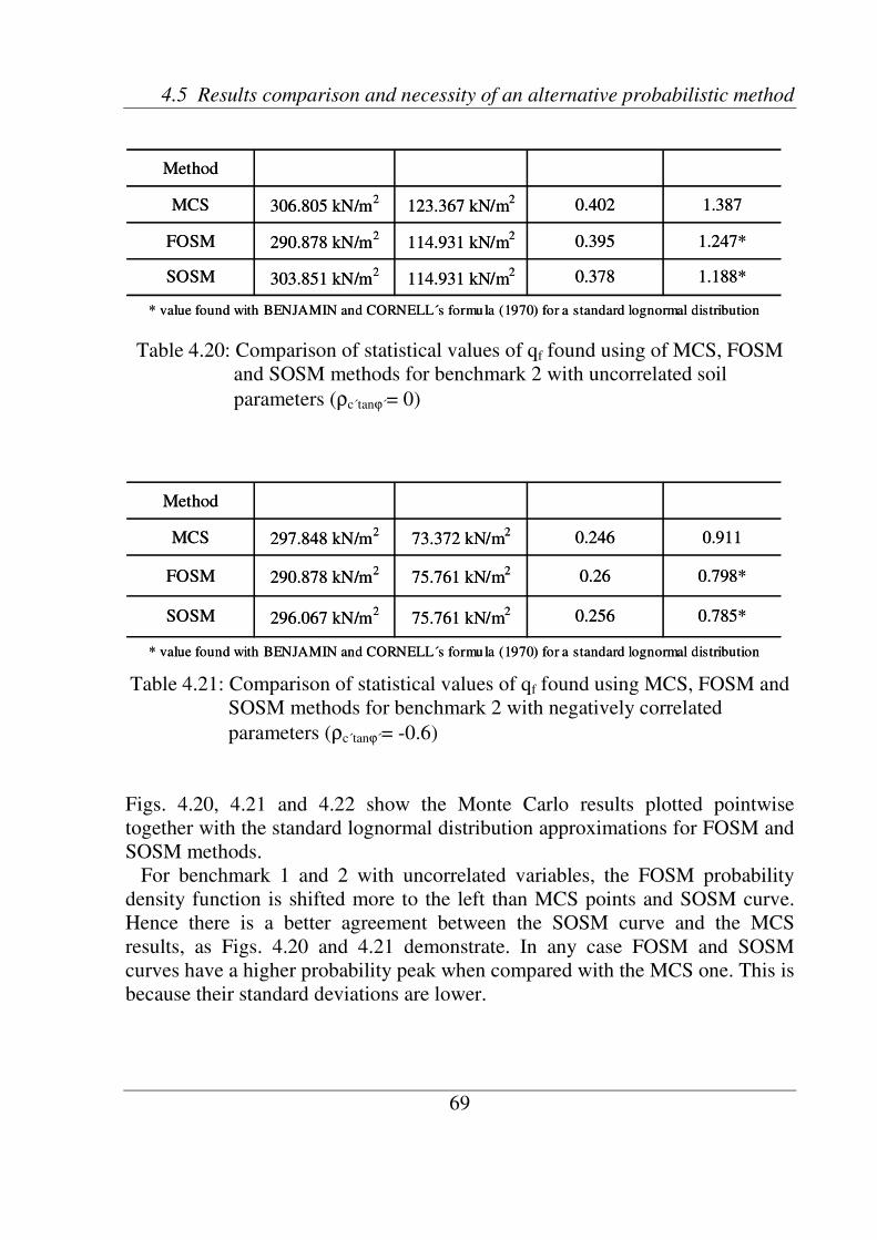
4.5 Results comparison and necessity of an alternative probabilistic method
69
1.247*
SOSM 303.851 kN/m2
114.931 kN/m2 0.378 1.188*
FOSM 290.878 kN/m2
114.931 kN/m2 0.395
MCS 306.805 kN/m2
123.367 kN/m2 0.402 1.387
Method
* value found with BENJAMIN and CORNELL´s formula (1970) for a standard lognormal distribution
1.247*
SOSM 303.851 kN/m2
114.931 kN/m2 0.378 1.188*
FOSM 290.878 kN/m2
114.931 kN/m2 0.395
MCS 306.805 kN/m2
123.367 kN/m2 0.402 1.387
Method
* value found with BENJAMIN and CORNELL´s formula (1970) for a standard lognormal distribution
0.798*
SOSM 296.067 kN/m2
75.761 kN/m2 0.256 0.785*
FOSM 290.878 kN/m2
75.761 kN/m2 0.26
MCS 297.848 kN/m2
73.372 kN/m2 0.246 0.911
Method
* value found with BENJAMIN and CORNELL´s formula (1970) for a standard lognormal distribution
0.798*
SOSM 296.067 kN/m2
75.761 kN/m2 0.256 0.785*
FOSM 290.878 kN/m2
75.761 kN/m2 0.26
MCS 297.848 kN/m2
73.372 kN/m2 0.246 0.911
Method
* value found with BENJAMIN and CORNELL´s formula (1970) for a standard lognormal distribution
Table 4.20: Comparison of statistical values of qf found using of MCS, FOSM
and SOSM methods for benchmark 2 with uncorrelated soil
parameters (ρc´tanϕ´= 0)
Table 4.21: Comparison of statistical values of qf found using MCS, FOSM and
SOSM methods for benchmark 2 with negatively correlated
parameters (ρc´tanϕ´= -0.6)
Figs. 4.20, 4.21 and 4.22 show the Monte Carlo results plotted pointwise
together with the standard lognormal distribution approximations for FOSM and
SOSM methods.
For benchmark 1 and 2 with uncorrelated variables, the FOSM probability
density function is shifted more to the left than MCS points and SOSM curve.
Hence there is a better agreement between the SOSM curve and the MCS
results, as Figs. 4.20 and 4.21 demonstrate. In any case FOSM and SOSM
curves have a higher probability peak when compared with the MCS one. This is
because their standard deviations are lower.

Chapter 4 Probabilistic analysis of the bearing capacity problem
70
0
0.0005
0.001
0.0015
0.002
0.0025
0.003
0.0035
0.004
0.0045
0 100 200 300 400 500 600 700 800
Bearing capacity qf (kN/m²)
Prob
ab
ilit
yd
en
sity
fun
cti
on
FOSM SOSM MCS
0tanc =ρϕ′′
0
0.0005
0.001
0.0015
0.002
0.0025
0.003
0.0035
0.004
0.0045
0 100 200 300 400 500 600 700 800
Bearing capacity qf (kN/m²)
Prob
ab
ilit
yd
en
sity
fun
cti
on
FOSM SOSM MCS
0
0.0005
0.001
0.0015
0.002
0.0025
0.003
0.0035
0.004
0.0045
0 100 200 300 400 500 600 700 800
Bearing capacity qf (kN/m²)
Prob
ab
ilit
yd
en
sity
fun
cti
on
FOSM SOSM
0
0.0005
0.001
0.0015
0.002
0.0025
0.003
0.0035
0.004
0.0045
0 100 200 300 400 500 600 700 800
Bearing capacity qf (kN/m²)
Prob
ab
ilit
yd
en
sity
fun
cti
on
FOSM SOSM MCS
0tanc =ρϕ′′
Figure 4.20: Comparison of MCS, FOSM and SOSM results in terms of
probability distribution for benchmark 1
Figure 4.21: Comparison of MCS, FOSM and SOSM results in terms of
probability distribution for benchmark 2 considering
uncorrelated soil variables.
0
0.0005
0.001
0.0015
0.002
0.0025
0.003
0.0035
0.004
0.0045
0.005
0 100 200 300 400 500 600 700 800
Bearing capacity qf
(kN/m²)
Prob
ab
ilit
yd
en
sity
fun
cti
on
FOSM SOSM MCS
0
0.0005
0.001
0.0015
0.002
0.0025
0.003
0.0035
0.004
0.0045
0.005
0 100 200 300 400 500 600 700 800
Bearing capacity qf
(kN/m²)
Prob
ab
ilit
yd
en
sity
fun
cti
on
FOSM
0
0.0005
0.001
0.0015
0.002
0.0025
0.003
0.0035
0.004
0.0045
0.005
0 100 200 300 400 500 600 700 800
Bearing capacity qf
(kN/m²)
Prob
ab
ilit
yd
en
sity
fun
cti
on
FOSM SOSM MCS
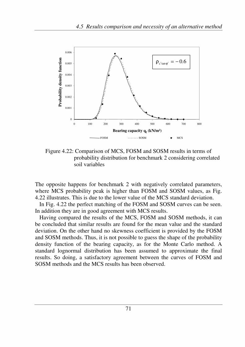
4.5 Results comparison and necessity of an alternative method
71
0
0.001
0.002
0.003
0.004
0.005
0.006
0 100 200 300 400 500 600 700 800
Bearing capacity qf
(kN/m²)
Prob
ab
ilit
yd
ensi
tyfu
ncti
on
FOSM SOSM MCS
6.0tanc −=ρϕ′′
0
0.001
0.002
0.003
0.004
0.005
0.006
0 100 200 300 400 500 600 700 800
Bearing capacity qf
(kN/m²)
Prob
ab
ilit
yd
ensi
tyfu
ncti
on
FOSM SOSM MCS
0
0.001
0.002
0.003
0.004
0.005
0.006
0 100 200 300 400 500 600 700 800
Bearing capacity qf
(kN/m²)
Prob
ab
ilit
yd
ensi
tyfu
ncti
on
FOSM SOSM MCS
6.0tanc −=ρϕ′′
Figure 4.22: Comparison of MCS, FOSM and SOSM results in terms of
probability distribution for benchmark 2 considering correlated
soil variables
The opposite happens for benchmark 2 with negatively correlated parameters,
where MCS probability peak is higher than FOSM and SOSM values, as Fig.
4.22 illustrates. This is due to the lower value of the MCS standard deviation.
In Fig. 4.22 the perfect matching of the FOSM and SOSM curves can be seen.
In addition they are in good agreement with MCS results.
Having compared the results of the MCS, FOSM and SOSM methods, it can
be concluded that similar results are found for the mean value and the standard
deviation. On the other hand no skewness coefficient is provided by the FOSM
and SOSM methods. Thus, it is not possible to guess the shape of the probability
density function of the bearing capacity, as for the Monte Carlo method. A
standard lognormal distribution has been assumed to approximate the final
results. So doing, a satisfactory agreement between the curves of FOSM and
SOSM methods and the MCS results has been observed.

Chapter 4 Probabilistic analysis of the bearing capacity problem
72
4.5.2 Necessity of an alternative probabilistic method
It was seen in chapter 3 that the Monte Carlo approach is the most reliable
technique between other well-known probabilistic methods, because not only
mean value, standard deviation and skewness coefficient of a performance
function can be estimated, but also the corresponding probability density
function can be identified. However, as already seen in chapter 3, for
geotechnical problems without an analytical solution, additional special
programming for the MCS would be needed. Furthermore, to obtain a high
accuracy, a large number of simulations are involved. Thus, in practice, this
method requires a very high computational effort.
FOSM and SOSM methods were then chosen as alternative probabilistic
approaches to replace MCS, both of which require only a limited amount of
calculations. However these methods are accurate only for linear functions. The
accuracy diminishes as the non-linearity of a function increases. In fact in this
chapter it has been pointed out that the bearing capacity varies exponentially
with tanϕ´. Thus, using FOSM and SOSM methods for a probabilistic analysis
of the bearing capacity problem, uncertainty is introduced in the calculations,
giving less accurate results than MCS.
It has been observed that the SOSM method seems to refine the estimate of the
bearing capacity mean value found by the FOSM method. However results show
that the improvement is small and hardly worthwhile for the proposed
benchmarks.
In addition these approaches require the computation and evaluation of partial
derivatives. This could be exceedingly difficult or impossible for many
problems, such as when relationships are only in the form of charts or graphics
or for solutions involving finite element methods. Furthermore no skewness
coefficient is provided by both these methods. For this reason no information
about the shape of the probability density function of the output is given. It has
to be assumed, thus introducing a source of inaccuracy.
Hence it is necessary to take into account another alternative, which can
overcome the drawbacks of MCS, FOSM and SOSM methods, providing a
skewness coefficient value together with the other statistical estimates, but with
less computational effort.
In chapter 5 the Two Point Estimate Method (PEM) will be chosen as
alternative approach to be applied to the bearing capacity benchmarks. The
results will be then presented and compared to those of the MCS, FOSM and
SOSM methods.
Although the PEM does not provide a full distribution of the output variable,
as Monte Carlo does, it will show to be a simple but powerful technique for

4.5 Results comparison and necessity of an alternative probabilistic method
73
probabilistic analyses, as it requires less computational effort than MCS for a
comparable degree of accuracy.
Moreover the PEM will provide not only mean value and standard deviation,
but also the skewness coefficient of the bearing capacity, giving then more
accurate results than FOSM and SOSM methods, with little or no increase in
computational effort and without evaluation of partial derivatives.
In chapter 6 the PEM will be applied for the evaluation of the failure probability
of the bearing capacity problem. It will be shown that also this method has some
limitations, as already mentioned in chapter 3.
However, despite its limitations, the PEM will proof to be a more attractive
method than MCS, from a computational point of view, and than FOSM and
SOSM approaches, as it will overcome their drawbacks.


75
Chapter 5
The Two Point Estimate method applied to
the bearing capacity problem
Introduction It has been shown in chapter 3 that various probabilistic methods exist to
quantify uncertainty. The most common are Monte Carlo simulations and the
moments methods FOSM and SOSM. However these approaches present
important shortcomings, as described in chapter 3 and demonstrated in chapter
4. These difficulties can be overcome, with some limitations, using the Two
Point Estimate Method after ROSENBLUETH (1975, 1981), described in
chapter 3.
In the present chapter, the PEM is applied to the bearing capacity problem.
The PEM results are then compared with those of the MCS, FOSM and SOSM
methods.
5.1 PEM results for benchmark 1
In order to assess the bearing capacity statistical values related to the first
benchmark, illustrated in chapter 4, the Two Point Estimate method after
ROSENBLUETH (1975) is applied. The procedure for implementing the PEM
and the corresponding calculations are described step by step in next section.
5.1.1 Procedure of the PEM
1. The relationship (4.6) between the dependent variable qf and the single
random variable tanϕ´ is considered.
2. The two sampling point locations for tanϕ´, which is normally distributed
( 0tan
=νϕ′
), have to be computed. First of all, the standard deviation units, giving
locations of the sampling points to the right and to the left of the mean value, are
evaluated using Eqs. (3.6), thus giving

Chapter 5 The Two Point Estimate method applied to the bearing capacity problem
76
f(tanφ´)
ϕ′µ
tan
f(tanφ´)
0+
ϕ′tan−
ϕ′tanϕ′tan
+ϕ′tanP−ϕ′tanP
f(tanφ´)
ϕ′µ
tan ϕ′µ
tan
f(tanφ´)
0+
ϕ′tan−
ϕ′tanϕ′tan
+ϕ′tanP−ϕ′tanP
1tantan
=ξ=ξ−ϕ′+ϕ′
.
Then the corresponding sampling point locations can be found by using Eqs.
(3.7), thus obtaining
406.0tan =ϕ′−
527.0tan =ϕ′+
.
Figure 5.1 shows the sampling points located at −
ϕ′tan and +
ϕ′tan .
3. Then the weights Pi are determined. In this case there is only one input
variable, for this reason no correlation coefficient is considered in the weights
formula. For tanϕ´ the weights are simply given by formula (3.8) and, because
of the symmetry of the normal distribution, they will have the same value, i.e.:
5.0PPtantan
==−ϕ′+ϕ′
.
4. The values of the bearing capacity are then evaluated at both sampling point
locations of tanϕ´. The results are shown in Table 5.1.
Figure 5.1: Sampling point locations and weights for tanϕ´

5.1 PEM results for benchmark 1
77
fqµfqσ
fqCOVfqν
306.785 kN/m2
97.167 kN/m2 0.317 0
fqµfqσ
fqCOVfqν
306.785 kN/m2
97.167 kN/m2 0.317 0
403.953 kN/m2
0.5
0.5 0.527
0.406 209.619 kN/m2
±P
±ϕ′tan
±fq
403.953 kN/m2
0.5
0.5 0.527
0.406 209.619 kN/m2
±P
±ϕ′tan
±fq
Table 5.1: Weights and sampling points of tanϕ´ and bearing capacity values for
PEM
5. Now the first three moments of the bearing capacity can be evaluated using
Eqs. (3.15), (3.16) and (3.17), where n = 1.
The results of the bearing capacity predicted by PEM are presented in Table
5.2. From this table, it can be seen that the mean value is 6.2% higher than the
deterministic value (i.e. 287.6 kN/m2). In addition the skewness coefficient is
nil, thus suggesting a symmetric probability density function for the bearing
capacity.
However, for a better definition of the shape of the bearing capacity
distribution more sampling points would be needed.
Assuming both a standard lognormal and a normal distribution, as suggested
by the skewness value in Table 5.2, the shape of the bearing capacity
distribution can be plotted for both cases obtaining the curves in Fig. 5.2.
In the literature (e.g. ANG and TANG, 1975; FENTON, 2006) it is frequently
reported that, for values of the variation coefficient lower than 30%, there is not
much difference between the shape of a normal and a lognormal distribution. On
the other hand, when the COV is higher than 30%, then a discrepancy exists
between the shape of these two important density functions. For the first
benchmark, the bearing capacity has a variation coefficient of approximately
32%, thus a certain discrepancy exists between the curves of Fig. 5.2.
Table 5.2: Statistical values of qf predicted by PEM
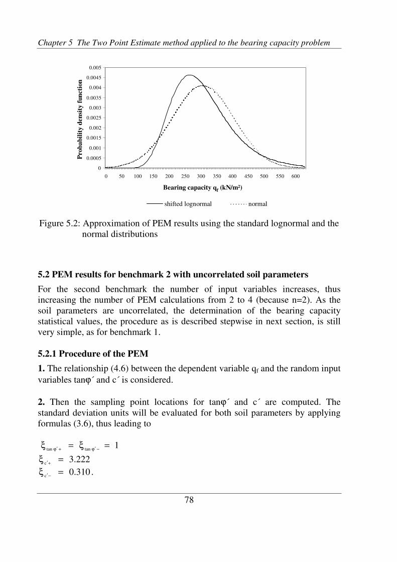
Chapter 5 The Two Point Estimate method applied to the bearing capacity problem
78
Figure 5.2: Approximation of PEM results using the standard lognormal and the
normal distributions
5.2 PEM results for benchmark 2 with uncorrelated soil parameters
For the second benchmark the number of input variables increases, thus
increasing the number of PEM calculations from 2 to 4 (because n=2). As the
soil parameters are uncorrelated, the determination of the bearing capacity
statistical values, the procedure as is described stepwise in next section, is still
very simple, as for benchmark 1.
5.2.1 Procedure of the PEM
1. The relationship (4.6) between the dependent variable qf and the random input
variables tanϕ´ and c´ is considered.
2. Then the sampling point locations for tanϕ´ and c´ are computed. The
standard deviation units will be evaluated for both soil parameters by applying
formulas (3.6), thus leading to
1tantan
=ξ=ξ−ϕ′+ϕ′
222.3c
=ξ+′
310.0c
=ξ−′
.
0
0.0005
0.001
0.0015
0.002
0.0025
0.003
0.0035
0.004
0.0045
0.005
0 50 100 150 200 250 300 350 400 450 500 550 600
Bearing capacity qf
(kN/m²)
Prob
ab
ilit
yd
en
sity
fun
cti
on
shifted lognormal normal
0
0.0005
0.001
0.0015
0.002
0.0025
0.003
0.0035
0.004
0.0045
0.005
0 50 100 150 200 250 300 350 400 450 500 550 600
Bearing capacity qf
(kN/m²)
Prob
ab
ilit
yd
en
sity
fun
cti
on
shifted lognormal normal

5.2 PEM results for benchmark 2 with uncorrelated soil parameters
79
f(tanφ´)
ϕ′µ
tan
f(tanφ´)
0+
ϕ′tan−
ϕ′tanϕ′tan
+ϕ′tanP−ϕ′tanP
f(c´)
c´c′
µ0+′c
−′c
+′cP
−′cPf(tanφ´)
ϕ′µ
tan ϕ′µ
tan
f(tanφ´)
0+
ϕ′tan−
ϕ′tanϕ′tan
+ϕ′tanP−ϕ′tanP
f(c´)
c´c′
µ0+′c
−′c
+′cP
−′cP
The corresponding sampling point locations can be evaluated with Eqs. (3.7)
527.0tan =ϕ′−
406.0tan =ϕ′+
2
m/kN311.14´c =+
2
m/kN007.3´c =−
.
3. The weights Pi, giving each of the four point estimates of soil parameters
considered as single random variable, are then determined using Eq. (3.8), thus
obtaining
5.0PPtantan
==−ϕ′+ϕ′
088.0Pc
=+′
912.0Pc
=−′
.
Figure 5.3 shows how the sampling points of both soil parameters tanϕ´ and c´
are located. The corresponding weights are also shown in these diagrams. Then
the associated weights need to be found, considering the input parameters as
multiple uncorrelated variables. Formula (3.9) gives the following weights:
044.0PPPctan
=⋅=+′+ϕ′++
456.0PPPctan
=⋅=−′+ϕ′−+
044.0PPPctan
=⋅=+′−ϕ′+−
456.0PPPctan
=⋅=−′−ϕ′−−
Figure 5.3: Sampling point locations and weights of the soil parameters tanϕ´
and c´

Chapter 5 The Two Point Estimate method applied to the bearing capacity problem
80
fqµfqσ
fqCOVfqν
306.786 kN/m2
119.236 kN/m2 0.389 0.912
fqµfqσ
fqCOVfqν
306.786 kN/m2
119.236 kN/m2 0.389 0.912
±±P
±ϕ′tan ±±fq
±′c
14.311 kN/m2 0.527 665.755 kN/m
2
3.007 kN/m2 0.527 378.740 kN/m
2
0.044
0.456
0.044 14.311 kN/m2 0.406 384.650 kN/m
2
0.456 3.007 kN/m2 0.406 192.762 kN/m
2
±±P
±ϕ′tan ±±fq
±′c
14.311 kN/m2 0.527 665.755 kN/m
2
3.007 kN/m2 0.527 378.740 kN/m
2
0.044
0.456
0.044 14.311 kN/m2 0.406 384.650 kN/m
2
0.456 3.007 kN/m2 0.406 192.762 kN/m
2
14.311 kN/m2 0.527 665.755 kN/m
2
3.007 kN/m2 0.527 378.740 kN/m
2
0.044
0.456
0.044 14.311 kN/m2 0.406 384.650 kN/m
2
0.456 3.007 kN/m2 0.406 192.762 kN/m
2
4. The value of the bearing capacity at each sampling point can now be
evaluated. The results are shown in Table 5.3.
Table 5.3: Associated weights, sampling points and bearing capacity values for
tanϕ´ and c´
5. The mean value, variance and skewness coefficient of the bearing capacity
can be determined using Eqs. (3.15), (3.16) and (3.17), where n = 2. The results
of the statistical estimates of the bearing capacity predicted by PEM are
presented in Table 5.4.
Comparing these results with those of Table 5.2, it can be seen that the mean
value is constant, while the standard deviation increases. This also increases the
skewness and the variation coefficients. The higher standard deviation is due to
the consideration of the effective cohesion as input random variable, which
introduces more uncertainty in the final results. Moreover, it can be deduced
from the positive skewness coefficient that the probability density function of
the bearing capacity is no longer symmetric, as found in the first benchmark.
Table 5.4: Statistical values of qf predicted by PEM with uncorrelated soil
variables
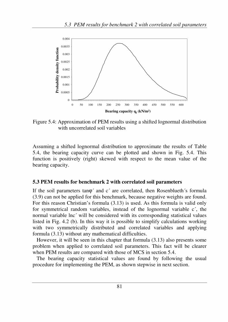
5.3 PEM results for benchmark 2 with correlated soil parameters
81
Figure 5.4: Approximation of PEM results using a shifted lognormal distribution
with uncorrelated soil variables
Assuming a shifted lognormal distribution to approximate the results of Table
5.4, the bearing capacity curve can be plotted and shown in Fig. 5.4. This
function is positively (right) skewed with respect to the mean value of the
bearing capacity.
5.3 PEM results for benchmark 2 with correlated soil parameters
If the soil parameters tanϕ´ and c´ are correlated, then Rosenblueth´s formula
(3.9) can not be applied for this benchmark, because negative weights are found.
For this reason Christian’s formula (3.13) is used. As this formula is valid only
for symmetrical random variables, instead of the lognormal variable c´, the
normal variable lnc´ will be considered with its corresponding statistical values
listed in Fig. 4.2 (b). In this way it is possible to simplify calculations working
with two symmetrically distributed and correlated variables and applying
formula (3.13) without any mathematical difficulties.
However, it will be seen in this chapter that formula (3.13) also presents some
problem when applied to correlated soil parameters. This fact will be clearer
when PEM results are compared with those of MCS in section 5.4.
The bearing capacity statistical values are found by following the usual
procedure for implementing the PEM, as shown stepwise in next section.
0
0.0005
0.001
0.0015
0.002
0.0025
0.003
0.0035
0.004
0 50 100 150 200 250 300 350 400 450 500 550 600
Bearing capacity qf
(kN/m²)
Prob
ab
ilit
yd
en
sity
fun
ctio
n
0
0.0005
0.001
0.0015
0.002
0.0025
0.003
0.0035
0.004
0 50 100 150 200 250 300 350 400 450 500 550 600
Bearing capacity qf
(kN/m²)
Prob
ab
ilit
yd
en
sity
fun
ctio
n

Chapter 5 The Two Point Estimate Method applied to the bearing capacity problem
82
ϕ′′ρ tancln
P++ P+- P-+ P--
-1.0 0.000 0.500 0.500 0.000
-0.9 0.025 0.475 0.475 0.025
-0.8 0.050 0.450 0.450 0.050
-0.7 0.075 0.425 0.425 0.075
-0.6 0.100 0.400 0.400 0.100
-0.5 0.125 0.375 0.375 0.125
-0.4 0.150 0.350 0.350 0.150
-0.3 0.175 0.325 0.325 0.175
-0.2 0.200 0.300 0.300 0.200
-0.1 0.225 0.275 0.275 0.225
0.0 0.250 0.250 0.250 0.250
Associated weightsϕ′′ρ tancln
P++ P+- P-+ P--
-1.0 0.000 0.500 0.500 0.000
-0.9 0.025 0.475 0.475 0.025
-0.8 0.050 0.450 0.450 0.050
-0.7 0.075 0.425 0.425 0.075
-0.6 0.100 0.400 0.400 0.100
-0.5 0.125 0.375 0.375 0.125
-0.4 0.150 0.350 0.350 0.150
-0.3 0.175 0.325 0.325 0.175
-0.2 0.200 0.300 0.300 0.200
-0.1 0.225 0.275 0.275 0.225
0.0 0.250 0.250 0.250 0.250
Associated weights
5.3.1 Procedure of the PEM
1. The relationship (4.6) between qf and the soil variables tanϕ´ and c´ is again
considered.
2. As tanϕ´ and lnc´ are both symmetrically distributed, then the standard
deviation units of the soil parameters will be both equal to unity. In fact Eqs.
(3.6) lead to
1tantan
=ξ=ξ−ϕ′+ϕ′
1clncln
=ξ=ξ−′+′
.
The sampling point locations for tanϕ´ and lnc´ are then computed by applying
formulas (3.7), thus obtaining
406.0tan =ϕ′−
527.0tan =ϕ′+
2
m/kN842.1´cln =+
2
m/kN436.0´cln =−
.
Table 5.5: Associated weights of tanϕ´ and lnc´ varying the correlation
coefficient
5.3 PEM results for benchmark 2 with correlated soil parameters
83
3. The weights Pi, giving each of the four point estimates of the soil parameters
considered as single random variable, are then determined using formula (3.8),
thus leading to
5.0PPtantan
==−ϕ′+ϕ′
5.0PPclncln
==−′+′
.
Formula (3.13) is then used to find the associated weights. The sampling
weights calculated for various correlation coefficients between 0 to –1.0 are
listed in Table 5.5.
4. To determine the bearing capacity values at each sampling point, the sampling
point locations of lnc´ need to be transformed into the sampling point locations
of the lognormal cohesion. This is done simply using the exponential function,
i.e.
2cln
m/kN311.6ec ==′ +′
+
2clnm/kN546.1ec ==′ −
′
−.
Then the relationship (4.6) can be easily applied to evaluate the bearing capacity
values listed in Table 5.6 for ρc´tanϕ´ = -0.6.
Eqs. (3.15), (3.16) and (3.17) can now be used to define the statistical values
of the bearing capacity corresponding to a correlation coefficient of –0.6. The
results are shown in Table 5.7.
Comparing results of Tables 5.4 and 5.7, one sees a slight change in the mean
value, while the standard deviation decreases down to around 35% when
compared with the value obtained considering uncorrelated soil parameters.
Consequently the skewness and the variation coefficients also decrease. Thus
the bearing capacity variability and the uncertainty in the analysis are strongly
reduced.
Assuming a shifted lognormal distribution and considering uncorrelated and
negatively correlated soil parameters with ρc´tanϕ´ = -0.6, the probability density
functions of the bearing capacity for both cases can be compared in one
diagram, as shown in Fig. 5.5. When uncorrelated variables are taken into
account then the density function shows a higher variability, being wider than
the curve for negatively correlated parameters. Also the peak values of these
distributions is clearly different, being around 0.0037 for the case with ρc´tanϕ´ = 0
and around 0.0052 for the case with ρc´tanϕ´ = -0.6.
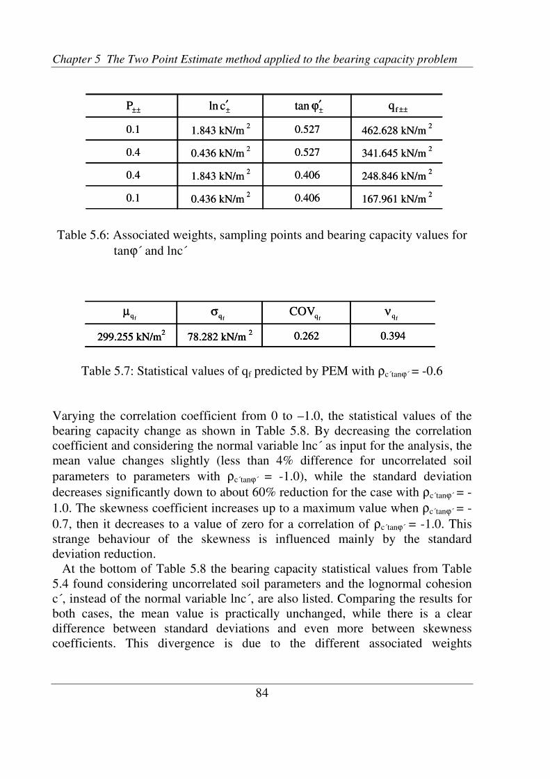
Chapter 5 The Two Point Estimate method applied to the bearing capacity problem
84
fqµfqσ
fqCOVfqν
299.255 kN/m2
78.282 kN/m2 0.262 0.394
fqµfqσ
fqCOVfqν
299.255 kN/m2
78.282 kN/m2 0.262 0.394299.255 kN/m
278.282 kN/m
2 0.262 0.394
±±P
±ϕ′tan ±±fq
±′cln
0.1 0.436 kN/m2 0.406 167.961 kN/m
2
0.4 1.843 kN/m2 0.406 248.846 kN/m
2
0.4 0.436 kN/m2 0.527 341.645 kN/m
2
0.1 1.843 kN/m2 0.527 462.628 kN/m
2
±±P
±ϕ′tan ±±fq
±′cln
0.1 0.436 kN/m2 0.406 167.961 kN/m
2
0.4 1.843 kN/m2 0.406 248.846 kN/m
2
0.4 0.436 kN/m2 0.527 341.645 kN/m
2
0.1 1.843 kN/m2 0.527 462.628 kN/m
2
Table 5.6: Associated weights, sampling points and bearing capacity values for
tanϕ´ and lnc´
Table 5.7: Statistical values of qf predicted by PEM with ρc´tanϕ´ = -0.6
Varying the correlation coefficient from 0 to –1.0, the statistical values of the
bearing capacity change as shown in Table 5.8. By decreasing the correlation
coefficient and considering the normal variable lnc´ as input for the analysis, the
mean value changes slightly (less than 4% difference for uncorrelated soil
parameters to parameters with ρc´tanϕ´ = -1.0), while the standard deviation
decreases significantly down to about 60% reduction for the case with ρc´tanϕ´ = -
1.0. The skewness coefficient increases up to a maximum value when ρc´tanϕ´ = -
0.7, then it decreases to a value of zero for a correlation of ρc´tanϕ´ = -1.0. This
strange behaviour of the skewness is influenced mainly by the standard
deviation reduction.
At the bottom of Table 5.8 the bearing capacity statistical values from Table
5.4 found considering uncorrelated soil parameters and the lognormal cohesion
c´, instead of the normal variable lnc´, are also listed. Comparing the results for
both cases, the mean value is practically unchanged, while there is a clear
difference between standard deviations and even more between skewness
coefficients. This divergence is due to the different associated weights

5.3 PEM results for benchmark 2 with correlated soil parameters
85
0
0.001
0.002
0.003
0.004
0.005
0.006
0 50 100 150 200 250 300 350 400 450 500 550 600
Bearing capacity qf(kN/m²)
Pro
bab
ilit
yd
ensi
tyfu
ncti
on
0tan =ρϕ′′c
6.0tan −=ρϕ′′c
0
0.001
0.002
0.003
0.004
0.005
0.006
0 50 100 150 200 250 300 350 400 450 500 550 600
Bearing capacity qf(kN/m²)
Pro
bab
ilit
yd
ensi
tyfu
ncti
on
0
0.001
0.002
0.003
0.004
0.005
0.006
0
0
0.001
0.002
0.003
0.004
0.005
0.006
0 50 100 150 200 250 300 350 400 450 500 550 600
Bearing capacity qf(kN/m²)
Pro
bab
ilit
yd
ensi
tyfu
ncti
on
0tan =ρϕ′′c
6.0tan −=ρϕ′′c
evaluated, respectively, by Eq. (3.9) for c´ and Eq. (3.13) for lnc´, which are
listed in Tables 5.3 and 5.6.
Unfortunately Rosenblueth´s formula can not be applied for benchmark 2 to
estimate any statistical values of the bearing capacity considering different
correlation coefficients, because, as already mentioned, negative associated
weights are found. Also Christian’s formulas can only be used when the normal
variable lnc´ is taken into account, because this formula refers only to
symmetrically distributed variables.
Hence the results of Table 5.8 referred to negative correlation coefficients can
not be compared with other statistical values, as done for the case with
uncorrelated variables.
As the results of Table 5.8 are the outcome of the application of formulas
(3.13) using a mathematical trick for considering the input variable cohesion as
normally distributed, i.e. lnc´ instead of c´, then the correlation between the
input variables is different, thus influencing the values of the associated weights.
For this reason these results will be used as reference for further comparisons
with other probabilistic methods results only for the case with negatively
correlated variables. Whereas the statistical values of Table 5.4 will be
considered as reference for further comparisons in case of uncorrelated soil
parameters, i.e. when 0ctan
=ρ′ϕ′
. For these comparisons the author refers to
section 5.4.
Figure 5.5: Comparison of the probability density functions of qf with ρc´tanϕ´ = 0
and with ρc´tanϕ´ = -0.6

Chapter 5 The Two Point Estimate method applied to the bearing capacity problem
86
)/( 2mkNfqµ )/(
2mkN
fqσϕ′′ρ tanc fqν
-1.0 295.246 46.399 0.000
-0.9 296.248 56.122 0.318
-0.8 297.250 64.378 0.399
-0.7 298.253 71.675 0.409
-0.6 299.255 78.282 0.394
-0.5 300.258 84.361 0.369
-0.4 301.260 90.020 0.340
-0.3 302.263 95.333 0.309
-0.2 303.265 100.354 0.280
-0.1 304.268 105.127 0.251
0.0 (considering lnc´) 305.270 109.683 0.223
0.0 (considering c´) 306.785 119.236 0.912
Table 5.8: Statistical values of the bearing capacity for different correlation
coefficients
Fig. 5.6 shows the influence of the correlation coefficient variation on the shape
of the shifted lognormal fit of the bearing capacity. As already pointed out for
Fig. 5.5, the curves become narrower for lower correlation coefficients, thus
decreasing the bearing capacity variability, which means less uncertainty in the
analysis. As a consequence the distribution peaks increase.
It should be noted that, for 0.1ctan
−=ρ′ϕ′
, the skewness coefficient of the
bearing capacity is nil, as reported in Table 5.8, meaning a symmetrical
distribution. For this reason a Gaussian distribution is assumed for plotting the
bearing capacity function in Fig. 5.6.
In this Figure the curve for 0ctan
=ρ′ϕ′
taking into account the lognormal
cohesion c´ as input variable is also plotted. Comparing this curve to that
obtained considering the normal variable lnc´ instead of c´, a clear divergence is
seen. The curve referred to c´ is in fact wider because of the higher standard
deviation. Furthermore, it is shifted more to the left because of the extremely
higher positive skewness coefficient.
Summarising it is possible to conclude that the choice of a negative correlation
between soil parameters is reasonable, because the uncertainty in the
probabilistic analysis is effectively reduced.

5.3 PEM results for benchmark 2 with correlated soil parameters
87
0
0.001
0.002
0.003
0.004
0.005
0.006
0.007
0.008
0.009
0.01
0 30 60 90 120 150 180 210 240 270 300 330 360 390 420 450 480 510 540 570 600 700
Bearing capacity qf (kN/m²)
Pro
ba
bil
ity
den
sity
fun
cti
on
0 (with lnc´) 0 (with c´) -0.1 -0.2 -0.3 -0.4
-0.5 -0.6 -0.7 -0.8 -0.9 -1
0
0.001
0.002
0.003
0.004
0.005
0.006
0.007
0.008
0.009
0.01
0 30 60 90 120 150 180 210 240 270 300 330 360 390 420 450 480 510 540 570 600 700
Bearing capacity qf (kN/m²)
Pro
ba
bil
ity
den
sity
fun
cti
on
0 (with lnc´) 0 (with c´) -0.1 -0.2 -0.3 -0.4
-0.5 -0.6 -0.7 -0.8 -0.9 -1
In addition it is shown in Table 5.8 and Fig. 5.6 that, depending on the weights
formula applied for benchmark 2 with uncorrelated soil variables, the bearing
capacity results are different, particularly in terms of skewness coefficient, thus
producing some difficulty in the interpretation of the outcome.
As already mentioned in chapter 3, ROSENBLUETH (1981) noted that when
multiple random variables are taken into account in the application of the PEM,
the value of the skewness coefficient can only be reliably calculated using Eq.
(3.17) if the variables are uncorrelated. Also CHRISTIAN and BAECHER
(1999) pointed out that the PEM should not be applied for evaluating the
skewness coefficient for non-linear functions, as in the case of the bearing
capacity formula.
Moreover, they observed that the larger the variation coefficient of the input
variables, the larger is the error in the estimates. In this study a variation
coefficient of 80% is considered for the cohesion. This value is higher than the
values usually found in the literature, thus introducing some inaccuracy in the
probabilistic results of the bearing capacity.
Figure 5.6: Influence of the correlation coefficient variation on the probability
distribution of the bearing capacity
Chapter 5 The Two Point Estimate Method applied to the bearing capacity problem
88
Finally, these authors stated that one should be careful when applying the PEM
to cases in which the transformation of an input variable changes its
distributional form, as it was done for the cohesion, for which important
information on the correlation coefficient between shear strength parameters is
lost. All these facts are confirmed in this chapter.
Thus, before applying a certain formula for evaluating the associated weights,
one should be aware of the characteristics of the input variables, i.e. if these are
symmetrically distributed or not and if a certain correlation exists between them.
5.4 Comparison of PEM, MCS, FOSM and SOSM results
The scope of this section is to compare PEM results for benchmark 1 and 2
already shown in chapter 4 to those of FOSM and SOSM methods, using the
Monte Carlo approach as a reference for the comparison.
In chapters 3 and 4 it has been shown that MCS are too time consuming for
practical purposes, which means consequently too expensive. Moreover, the
FOSM and SOSM methods do not provide information about the skewness
coefficient.
The PEM is chosen as alternative probabilistic method to be applied to the
bearing capacity problem, instead of MCS, FOSM and SOSM methods, because
it requires much less computational effort than MCS and it also provides
information about the skewness coefficient. Furthermore this approach does not
require the determination and evaluation of partial derivatives of the bearing
capacity formula as FOSM and SOSM, thus being more straightforward to use.
Nevertheless, as already discussed in section 5.3, the PEM has also some
drawbacks. These are highlighted in this section when the skewness coefficients
of MCS and PEM methods are compared.
5.4.1 Comparison of results for benchmark 1
In Table 5.9 the statistical values of the bearing capacity for benchmark 1 found
by applying the probabilistic methods PEM, FOSM, SOSM and MCS are listed.
Mean values, standard deviations and, consequently, variation coefficients are
quite similar, while a significant difference is observed between the skewness
coefficients. In fact the FOSM and SOSM method do not provide any skewness
coefficient, while the PEM provides a nil value. Thus the PEM is more accurate
than FOSM and SOSM methods, giving the additional information about the
shape of the bearing capacity distribution. However this value is extremely
different from the skewness coefficient found by MCS, which is 1.008.

5.4 Comparison of PEM, MCS, FOSM and SOSM results
89
Assuming a standard lognormal distribution, the probability density function of
PEM, FOSM and SOSM results can be drawn together with the results derived
from 10000 MCS plotted pointwise, as shown in Fig. 5.7.
Actually, the PEM skewness coefficient suggests that a normal distribution
should be assumed for approximating the bearing capacity statistical values.
However, following the conclusions reported in section 5.1 about the variation
coefficient and referring to Fig. 5.2, a standard lognormal distribution is
preferred, because it seems to be more representative for the bearing capacity.
Despite the different skewness coefficient, the PEM curve matches very well
the points indicating the MCS results, even if PEM distribution is a little bit
skewed to the right and up. Hence PEM apparently seems to be insensitive to the
skewness and gives virtually the same distribution as the computationally not so
attractive MCS.
It is important to observe that PEM requires only two calculations, against the
10000 simulations for Monte Carlo method, to get the results of Table 5.9. Thus,
by applying PEM, the computational effort considerably decreases.
Considering Benjamin and Cornell’s formula (4.1) valid for a standard
lognormal distribution, it is possible to assign fictitious skewness coefficients
for the FOSM and SOSM results. These values are then compared with the
skewness coefficient found by PEM and MCS, as shown in Table 5.9. These
fictitious values are very similar to the skewness coefficient found by MCS,
whereas they are extremely different from the value of PEM. Nevertheless,
because a standard lognormal distribution is assumed as approximation for the
PEM results, it is then possible to determine a fictitious skewness also for this
method. The value is approximately 0.983 and it is similar to the fictitious
skewness coefficients assigned to FOSM and SOSM methods and to the
skewness coefficient of the MCS. For this reason the curves in Fig. 5.7 are in
good agreement. However, the FOSM curve is skewed more to left due to the
lower mean value. If another type of distribution were to be assumed for
approximating the results of Table 5.9, then the fictitious skewness coefficients
would also change.
For more detail about the assumption of different distribution functions as an
approximation for the probabilistic results of the bearing capacity the author
refers to section 5.5. For example, by assuming a Gaussian distribution, the
skewness coefficients of all probabilistic approaches would be the same. The
difference reported in Table 5.9 for the skewness would then disappear.
However, the author would like to point out that one of the goal of this work is
to find the most suitable probability distribution which approximates MCS and
PEM results best and not those of FOSM and SOSM methods.

Chapter 5 The Two Point Estimate Method applied to the bearing capacity problem
90
fqµfqσ
fqCOVfqν
MCS
SOSM
FOSM
PEM
Method
1.003*
303.851 kN/m2
93.876 kN/m2 0.309 0.956*
290.878 kN/m2
93.876 kN/m2 0.323
306.785 kN/m2
97.167 kN/m2 0.317 0
1.008306.562 kN/m2
102.242 kN/m2 0.333
*value found with BENJAMIN and CORNELL´s formula (1970) for a standard lognormal
distribution
Table 5.9: Statistical values of qf found using PEM, FOSM, SOSM and MCS
methods
Figure 5.7: Comparison of PEM, FOSM, SOSM and MCS results in terms of
probability density function
From this results comparison it would seem that no real advantage exists by
applying PEM or FOSM and SOSM method, as PEM does not provide a
0
0.0005
0.001
0.0015
0.002
0.0025
0.003
0.0035
0.004
0.0045
0.005
0 100 200 300 400 500 600 700
Bearing capacity qf (kN/m²)
Pro
ba
bil
ity
den
sity
fun
ctio
n
FOSM SOSM PEM MCS
0
0.0005
0.001
0.0015
0.002
0.0025
0.003
0.0035
0.004
0.0045
0.005
0 100 200 300 400 500 600 700
Bearing capacity qf (kN/m²)
Pro
ba
bil
ity
den
sity
fun
ctio
n
FOSM SOSM PEM MCS
5.4 Comparison of PEM, MCS, FOSM and SOSM results
91
meaningful skewness coefficient for benchmark 1 as compared with the MCS
results.
However it will be seen in next sections that PEM, not only strongly decreases
the number of calculations, but can give more significant skewness values when
multiple input variables are considered, as for benchmark 2, where both
cohesion and tanϕ´ are taken into account.
Nevertheless, some difficulty will be encountered in the evaluation of the
skewness when correlated soil variables are considered.
5.4.2 Comparison of results for benchmark 2 with uncorrelated soil
parameters
Table 5.10 summarizes the statistical values of the bearing capacity previously
evaluated by PEM, FOSM, SOSM and MCS methods for benchmark 2
considering uncorrelated soil parameters. Comparing these results, it can be seen
that mean values and standard deviations are quite similar, while there is a
difference between the skewness coefficients. However, when compared with
the results of benchmark 1 in Table 5.9, the difference between MCS and PEM
skewness coefficient is now decreased down to about 35%, instead of the earlier
100%.
Considering a standard lognormal distribution and using again formula (4.1),
fictitious skewness coefficients can be assigned to the FOSM and SOSM
methods, which are listed in Table 5.10. In contrast to benchmark 1, these values
are similar to the skewness coefficient of the PEM. This is certainly due to the
introduction of the cohesion c´ as additional input variable, whose skewness
strongly influences that of the bearing capacity. Of course if another distribution
were to be assumed for approximating the FOSM and SOSM results, then other
skewness values would be found.
Assuming a shifted lognormal distribution for PEM and a standard lognormal
distribution for FOSM and SOSM methods, then the results of Table 5.10 can be
drawn in Fig. 5.8 together with MCS results plotted pointwise. When compared
with benchmark 1, the PEM curve is now more skewed right down than those of
FOSM and SOSM methods, due to the fact that a shifted lognormal, and not a
standard lognormal distribution is assumed as an approximation.
If a standard lognormal distribution were to be assumed for plotting PEM
results, then this difference would disappear. The fictitious skewness coefficient
of the PEM of approximately 1.226 is very similar to the FOSM, SOSM and
MCS values and all the fitting curves would be then in good agreement.
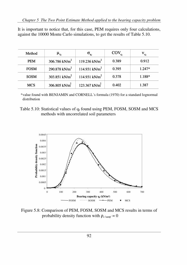
Chapter 5 The Two Point Estimate Method applied to the bearing capacity problem
92
fqµfqσ
fqCOVfqν
MCS
SOSM
FOSM
PEM
Method
306.805 kN/m2
123.367 kN/m2
0.402 1.387
1.247*
303.851 kN/m2
114.931 kN/m2 0.378 1.188*
290.878 kN/m2
114.931 kN/m2 0.395
306.786 kN/m2
119.236 kN/m2 0.389 0.912
fqµfqσ
fqCOVfqν
MCS
SOSM
FOSM
PEM
Method
306.805 kN/m2
123.367 kN/m2
0.402 1.387
1.247*
303.851 kN/m2
114.931 kN/m2 0.378 1.188*
290.878 kN/m2
114.931 kN/m2 0.395
306.786 kN/m2
119.236 kN/m2 0.389 0.912
It is important to notice that, for this case, PEM requires only four calculations,
against the 10000 Monte Carlo simulations, to get the results of Table 5.10.
*value found with BENJAMIN and CORNELL´s formula (1970) for a standard lognormal
distribution
Table 5.10: Statistical values of qf found using PEM, FOSM, SOSM and MCS
methods with uncorrelated soil parameters
Figure 5.8: Comparison of PEM, FOSM, SOSM and MCS results in terms of
probability density function with ρc´tanϕ´ = 0
0
0.0005
0.001
0.0015
0.002
0.0025
0.003
0.0035
0.004
0.0045
0 100 200 300 400 500 600 700
Bearing capacity qf (kN/m²)
Pro
ba
bil
ity
den
sity
fun
ctio
n
FOSM SOSM PEM MCS
0
0.0005
0.001
0.0015
0.002
0.0025
0.003
0.0035
0.004
0.0045
0 100 200 300 400 500 600 700
Bearing capacity qf (kN/m²)
Pro
ba
bil
ity
den
sity
fun
ctio
n
FOSM SOSM PEM MCS

5.4 Comparison of PEM, MCS, FOSM and SOSM results
93
fqµfqσ
fqCOVfqν
MCS
SOSM
FOSM
PEM
Method
0.911297.848 kN/m2
73.372 kN/m2 0.246
0.798*
296.067 kN/m2
75.761 kN/m2 0.256 0.785*
290.878 kN/m2
75.761 kN/m2
0.26
299.255 kN/m2
78.282 kN/m2 0.262 0.394
fqµfqσ
fqCOVfqν
MCS
SOSM
FOSM
PEM
Method
0.911297.848 kN/m2
73.372 kN/m2 0.246
0.798*
296.067 kN/m2
75.761 kN/m2 0.256 0.785*
290.878 kN/m2
75.761 kN/m2
0.26
299.255 kN/m2
78.282 kN/m2 0.262 0.394
5.4.3 Comparison of results for benchmark 2 with correlated soil
parameters
The statistical values of the bearing capacity found by applying PEM, FOSM,
SOSM and MCS methods to benchmark 2 taking into account a negative
correlation of ρc´tanϕ´ = -0.6 are listed in Table 5.11. Mean values and standard
deviations are quite similar, even considering a correlation between input
variables. On the other hand, a significant discrepancy exists between skewness
coefficients.
In fact FOSM and SOSM methods do not provide any value, while the
skewness coefficient of the PEM is about 60% lower than MCS value. This
difference is due to the inconvenience of applying PEM formulas (3.13) to the
non-symmetric variable c´, as described in section 5.3. In order to apply
Christian’s formula to evaluate the associated weights, the normal variable lnc´
needs to be considered, thus influencing the correlation coefficient between
cohesion and friction angle, because of the different mean value and standard
deviation of lnc´ and c´.
Assuming a shifted lognormal distribution for PEM and a standard lognormal
distribution for FOSM and SOSM methods, then results of Table 5.11 can be
plotted in Fig. 5.9 together with MCS results. Despite the different skewness
coefficients, the curves are in good agreement.
*value found with BENJAMIN and CORNELL´s formula (1970) for a standard lognormal
distribution
Table 5.11: Statistical values of qf found using PEM, FOSM, SOSM and MCS
methods with ρc´tanϕ´ = -0.6

Chapter 5 The Two Point Estimate method applied to the bearing capacity problem
94
0
0.001
0.002
0.003
0.004
0.005
0.006
0 100 200 300 400 500 600 700
Bearing capacity qf (kN/m²)
Pro
bab
ilit
yd
ensi
tyfu
nct
ion
FOSM SOSM PEM MCS
0
0.001
0.002
0.003
0.004
0.005
0.006
0 100 200 300 400 500 600 700
Bearing capacity qf (kN/m²)
Pro
bab
ilit
yd
ensi
tyfu
nct
ion
FOSM SOSM PEM MCS
Figure 5.9: Comparison of PEM, FOSM, SOSM and MCS results in terms of
probability density function with ρc´tanϕ´ = -0.6
Benjamin and Cornell’s formula (4.1) is applied to evaluate a fictitious value for
the skewness coefficient of FOSM and SOSM methods, as reported in Table
5.11. Thus the skewness coefficients of all methods can be compared. One notes
that PEM skewness is around 50% lower than FOSM and SOSM fictitious
values, while the value of MCS is less than 15% higher. If another distribution
were to be assumed for approximating FOSM and SOSM results, then it would
be possible to find other skewness coefficients, maybe more similar to the PEM
or MCS values.
Also in this case, if a standard lognormal distribution were to be assumed for
approximating PEM results, then the fictitious skewness coefficient of PEM
would be approximately 0.804, which is very similar to the fictitious values
found for FOSM and SOSM methods and slightly lower than the MCS value.
5.5 Discussion of the assumption of the shifted lognormal distribution
The use of a certain probability density function in preference to others plays an
important role in the probabilistic analysis of the bearing capacity problem, as
shown in this chapter.
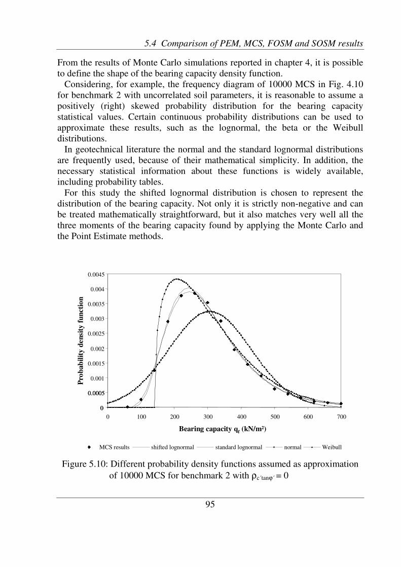
5.4 Comparison of PEM, MCS, FOSM and SOSM results
95
0
0.0005
0.001
0.0015
0.002
0.0025
0.003
0.0035
0.004
0.0045
0 100 200 300 400 500 600 700
Bearing capacity qf(kN/m²)
Pro
bab
ilit
yd
en
sity
fun
cti
on
MCS results shifted lognormal standard lognormal normal Weibull
0
0.0005
0
0.0005
0.001
0.0015
0.002
0.0025
0.003
0.0035
0.004
0.0045
0 100 200 300 400 500 600 700
Bearing capacity qf(kN/m²)
Pro
bab
ilit
yd
en
sity
fun
cti
on
MCS results shifted lognormal standard lognormal normal Weibull
From the results of Monte Carlo simulations reported in chapter 4, it is possible
to define the shape of the bearing capacity density function.
Considering, for example, the frequency diagram of 10000 MCS in Fig. 4.10
for benchmark 2 with uncorrelated soil parameters, it is reasonable to assume a
positively (right) skewed probability distribution for the bearing capacity
statistical values. Certain continuous probability distributions can be used to
approximate these results, such as the lognormal, the beta or the Weibull
distributions.
In geotechnical literature the normal and the standard lognormal distributions
are frequently used, because of their mathematical simplicity. In addition, the
necessary statistical information about these functions is widely available,
including probability tables.
For this study the shifted lognormal distribution is chosen to represent the
distribution of the bearing capacity. Not only it is strictly non-negative and can
be treated mathematically straightforward, but it also matches very well all the
three moments of the bearing capacity found by applying the Monte Carlo and
the Point Estimate methods.
Figure 5.10: Different probability density functions assumed as approximation
of 10000 MCS for benchmark 2 with ρc´tanϕ´ = 0

Chapter 5 The Two Point Estimate Method applied to the bearing capacity problem
96
The pointwise results of 10000 MCS for benchmark 2 considering ρc´tanϕ´ = 0 are
shown in Fig. 5.10 together with four possible fits using well-known probability
density functions.
A large discrepancy exists between the Gaussian normal distribution assumed
as approximation and the MCS results described pointwise. This is due to the
fact that the skewness coefficient evaluated using the Monte Carlo method is not
nil. Furthermore, as Fig. 5.10 shows, the Gaussian distribution allows negative
bearing capacity values, which are physically unrealistic. Then the Gaussian
distribution could only be seen as a rough approximation.
The Weibull distribution shows a good agreement with MCS results for values
of the bearing capacity higher than around qf = 270 kN/m2. However this curve
can not be a good fit because it does not describe the entire interval of the
bearing capacity variability as Monte Carlo method does. This curve is truncated
at about qf = 140 kN/m2.
The standard and the shifted lognormal distributions seem to approximate
MCS results at best. In fact the curves found considering these two distributions
match very well the points referred to the MCS results.
Figure 5.11: Different probability density functions assumed as approximation
for PEM results of benchmark 2 with ρc´tanϕ´ = 0
0
0.0005
0.001
0.0015
0.002
0.0025
0.003
0.0035
0.004
0.0045
0 50 100 150 200 250 300 350 400 450 500 550 600
Bearing capacity qf (kN/m²)
Pro
ba
bil
ity
den
sity
fun
ctio
n
shifted lognormal standard lognormal normal Weibull
0
0.0005
0.001
0.0015
0.002
0.0025
0.003
0.0035
0.004
0.0045
0 50 100 150 200 250 300 350 400 450 500 550 600
Bearing capacity qf (kN/m²)
Pro
ba
bil
ity
den
sity
fun
ctio
n
shifted lognormal standard lognormal normal Weibull

5.5 Discussion of the assumption of the shifted lognormal distribution
97
Moreover, looking at the first term of the bearing capacity formula (A.4) in
Appendix A, this is given as the product of the two input variables c´ and tanϕ´.
Hence, for the central limit theorem, the distribution of the bearing capacity
should tend to a lognormal distribution.
Apparently, it seems to be that the standard lognormal distribution is more
appropriate than the shifted one, especially around the peak of the curve.
Nevertheless only the shifted lognormal distribution can match the skewness
coefficient of the bearing capacity. This is why this function is preferred to
others as an approximation of the results of this probabilistic analysis.
Fig. 5.11 shows possible probability density functions assumed for
approximating PEM results of benchmark 2 considering uncorrelated soil
variables. In this diagram the good matching of the standard and the shifted
lognormal functions can be seen, while there is a high divergence between these
two curves and the Weibull and the Gaussian distributions.
It should be pointed out that the differences showed in Figs. 5.10 and 5.11
would become less important if the method of maximum likelihood would be
applied. However its results could not be directly compared to the results of the
other probabilistic methods considered for the bearing capacity problem, as the
method of maximum likelihood is not moment oriented.
Figs. 5.12 shows the comparison of the shifted lognormal (a), standard
lognormal (b), normal (c) and Weibull (d) distributions for MCS, PEM, FOSM
and SOSM results referred to benchmark 2 taking into account uncorrelated soil
parameters.
As the FOSM and SOSM methods do not provide any skewness, their results
can not be approximated by a shifted lognormal distribution, as this function
requires the knowledge of all the first three moments of the bearing capacity.
Thus in Fig. 5.12 a) only the curves for MCS and PEM results are plotted. These
have been already compared in section 5.4.2.
The fitting curves of Fig. 5.12 b) and c) seem to agree satisfactorily. However,
the assumption of a standard lognormal and of a normal distributions is not the
best choice. In fact the standard lognormal distribution does not match the real
skewness coefficients evaluated using MCS and PEM. Instead, fictitious
skewness values, estimated with formula (4.1), are assigned to these methods.
In addition, the Gaussian normal distribution allows negative bearing capacity
values for every probabilistic approach, which are physically impossible. In Fig.
5.12 c) these negative values do not appear, because the curves are truncated at
the origin.

Chapter 5 The Two Point Estimate method applied to the bearing capacity problem
98
0
0.0005
0.001
0.0015
0.002
0.0025
0.003
0.0035
0.004
0.0045
0 100 200 300 400 500 600 700
Pro
bab
ilit
yd
ensi
tyfu
nct
ion
MCS PEM
0
0.0005
0.001
0.0015
0.002
0.0025
0.003
0.0035
0.004
0.0045
0 100 200 300 400 500 600 700
Pro
bab
ilit
yd
ensi
tyfu
nct
ion
MCS PEM
Bearing capacity qf (kN/m²)
0
0.0005
0.001
0.0015
0.002
0.0025
0.003
0.0035
0.004
0.0045
0 100 200 300 400 500 600 700
Pro
ba
bil
ity
den
sity
fun
ctio
n
MCS PEM FOSM SOSM
0
0.0005
0.001
0.0015
0.002
0.0025
0.003
0.0035
0.004
0.0045
0 100 200 300 400 500 600 700
Pro
ba
bil
ity
den
sity
fun
ctio
n
MCS PEM FOSM SOSM
Bearing capacity qf (kN/m²)
a) b)
0
0.0005
0.001
0.0015
0.002
0.0025
0.003
0.0035
0.004
0.0045
0 100 200 300 400 500 600 700
Pro
ba
bil
ity
den
sity
fun
ctio
n
MCS PEM FOSM SOSM
0
0.0005
0.001
0.0015
0.002
0.0025
0.003
0.0035
0.004
0.0045
0 100 200 300 400 500 600 700
Pro
ba
bil
ity
den
sity
fun
ctio
n
MCS PEM FOSM SOSM
Bearing capacity qf (kN/m²)
c)
0
0.0005
0.001
0.0015
0.002
0.0025
0.003
0.0035
0.004
0.0045
0 100 200 300 400 500 600 700
Pro
ba
bil
ity
den
sity
fun
ctio
n
MCS PEM FOSM SOSM
0
0.0005
0.001
0.0015
0.002
0.0025
0.003
0.0035
0.004
0.0045
0 100 200 300 400 500 600 700
Pro
ba
bil
ity
den
sity
fun
ctio
n
MCS PEM FOSM SOSM
Bearing capacity qf (kN/m²)
d)
0
0.0005
0.001
0.0015
0.002
0.0025
0.003
0.0035
0.004
0.0045
0 100 200 300 400 500 600 700
Pro
bab
ilit
yd
ensi
tyfu
nct
ion
MCS PEM
0
0.0005
0.001
0.0015
0.002
0.0025
0.003
0.0035
0.004
0.0045
0 100 200 300 400 500 600 700
Pro
bab
ilit
yd
ensi
tyfu
nct
ion
MCS PEM
Bearing capacity qf (kN/m²)
0
0.0005
0.001
0.0015
0.002
0.0025
0.003
0.0035
0.004
0.0045
0 100 200 300 400 500 600 700
Pro
ba
bil
ity
den
sity
fun
ctio
n
MCS PEM FOSM SOSM
0
0.0005
0.001
0.0015
0.002
0.0025
0.003
0.0035
0.004
0.0045
0 100 200 300 400 500 600 700
Pro
ba
bil
ity
den
sity
fun
ctio
n
MCS PEM FOSM SOSM
Bearing capacity qf (kN/m²)
a) b)
0
0.0005
0.001
0.0015
0.002
0.0025
0.003
0.0035
0.004
0.0045
0 100 200 300 400 500 600 700
Pro
ba
bil
ity
den
sity
fun
ctio
n
MCS PEM FOSM SOSM
0
0.0005
0.001
0.0015
0.002
0.0025
0.003
0.0035
0.004
0.0045
0 100 200 300 400 500 600 700
Pro
ba
bil
ity
den
sity
fun
ctio
n
MCS PEM FOSM SOSM
Bearing capacity qf (kN/m²)
c)
0
0.0005
0.001
0.0015
0.002
0.0025
0.003
0.0035
0.004
0.0045
0 100 200 300 400 500 600 700
Pro
ba
bil
ity
den
sity
fun
ctio
n
MCS PEM FOSM SOSM
0
0.0005
0.001
0.0015
0.002
0.0025
0.003
0.0035
0.004
0.0045
0 100 200 300 400 500 600 700
Pro
ba
bil
ity
den
sity
fun
ctio
n
MCS PEM FOSM SOSM
Bearing capacity qf (kN/m²)
d)
Figure 5.12: Comparison of different probability density functions for MCS,
PEM, FOSM and SOSM results for benchmark 2 with ρc´tanϕ´ = 0:
a) shifted lognormal, b) standard lognormal, c) normal and
d) Weibull distributions
Finally one can see in Fig. 5.12 d) how the Weibull distribution presents the
largest discrepancy. In fact for FOSM and SOSM method, whose skewness
coefficient does not exist, the curves seem to be very similar to a normal
distribution, giving negative values for the bearing capacity, here truncated at
the origin.
On the other hand the well-known shape of the Weibull distribution with a
lower bound is clearer for MCS and PEM methods, for which the skewness
coefficient is not zero.
The Weibull curve for PEM results is wider, meaning more variability of the
bearing capacity, and with lower peak than the MCS function. This is mostly
due to the lower skewness coefficient of PEM results, as already seen in section
5.5 Discussion of the assumption of the shifted lognormal distribution
99
5.5.2 and shown in Fig. 5.12 a), when the assumption of the shifted lognormal
distribution is considered.
As described in Fig. 5.12, the probability density functions behaviour for the
bearing capacity results of benchmark 1 is shown in Fig. 5.13. However some
differences can be highlighted:
- In Fig. 5.13 a) only the MCS fit can be plotted. In fact to find the three
parameters of the shifted lognormal distribution using Eqs. (2.16), (2.17) and
(2.18), the skewness coefficient should be different to zero. This is not the case
for PEM results of benchmark 1, where the bearing capacity skewness is nil.
- In Fig. 5.13 b) and c), the density function referred to the MCS results, for a
lognormal and a normal distribution, is wider and has a lower peak when
compared with the other methods. In fact, by neglecting the real skewness
coefficient and because the standard deviation of MCS is larger than the values
of PEM, FOSM and SOSM methods, the variability of the bearing capacity will
be higher.
- Finally, when compared to Fig. 5.12 d), in Fig. 5.13 d) the PEM approximation
using the Weibull distribution seems to match well the FOSM and SOSM
curves. This is due to the value of the skewness coefficient, which is nil for
benchmark 1.
It should be pointed out that the differences showed in Figs. 5.10 and 5.11
would become less important if the method of maximum likelihood would be
applied. However its results could not be directly compared to the results of the
other probabilistic methods considered for the bearing capacity problem, as the
method of maximum likelihood is not moment oriented.
Figs. 5.12 shows the comparison of the shifted lognormal (a), standard
lognormal (b), normal (c) and Weibull (d) distributions for MCS, PEM, FOSM
and SOSM results referred to benchmark 2 taking into account uncorrelated soil
parameters.
As the FOSM and SOSM methods do not provide any skewness, their results
can not be approximated by a shifted lognormal distribution, as this function
requires the knowledge of all the first three moments of the bearing capacity.
Thus in Fig. 5.12 a) only the curves for MCS and PEM results are plotted. These
have been already compared in section 5.4.2.
The fitting curves of Fig. 5.12 b) and c) seem to agree satisfactorily. However,
the assumption of a standard lognormal and of a normal distributions is not the
best choice.

Chapter 5 The Two Point Estimate method applied to the bearing capacity problem
100
0
0.0005
0.001
0.0015
0.002
0.0025
0.003
0.0035
0.004
0.0045
0.005
0 100 200 300 400 500 600 700
Pro
ba
bil
ity
den
sity
fun
cti
on
MCS
0
0.0005
0.001
0.0015
0.002
0.0025
0.003
0.0035
0.004
0.0045
0.005
0 100 200 300 400 500 600 700
Pro
ba
bil
ity
den
sity
fun
cti
on
MCS
Bearing capacity qf (kN/m²)
a)
0
0.0005
0.001
0.0015
0.002
0.0025
0.003
0.0035
0.004
0.0045
0.005
0 100 200 300 400 500 600 700
Pro
ba
bil
ity
den
sity
fun
cti
on
MCS PEM FOSM SOSM
0
0.0005
0.001
0.0015
0.002
0.0025
0.003
0.0035
0.004
0.0045
0.005
0 100 200 300 400 500 600 700
Pro
ba
bil
ity
den
sity
fun
cti
on
MCS PEM FOSM SOSM
Bearing capacity qf (kN/m²)
b)
0
0.0005
0.001
0.0015
0.002
0.0025
0.003
0.0035
0.004
0.0045
0.005
0 100 200 300 400 500 600 700
Pro
ba
bil
ity
den
sity
fun
cti
on
MCS PEM FOSM SOSM
0
0.0005
0.001
0.0015
0.002
0.0025
0.003
0.0035
0.004
0.0045
0.005
0 100 200 300 400 500 600 700
Pro
ba
bil
ity
den
sity
fun
cti
on
MCS PEM FOSM SOSM
Bearing capacity qf (kN/m²)
c)
0
0.0005
0.001
0.0015
0.002
0.0025
0.003
0.0035
0.004
0.0045
0.005
0 100 200 300 400 500 600 700
Pro
ba
bil
ity
den
sity
fun
cti
on
MCS PEM FOSM SOSM
0
0.0005
0.001
0.0015
0.002
0.0025
0.003
0.0035
0.004
0.0045
0.005
0 100 200 300 400 500 600 700
Pro
ba
bil
ity
den
sity
fun
cti
on
MCS PEM FOSM SOSM
d)
Bearing capacity qf (kN/m²)
0
0.0005
0.001
0.0015
0.002
0.0025
0.003
0.0035
0.004
0.0045
0.005
0 100 200 300 400 500 600 700
Pro
ba
bil
ity
den
sity
fun
cti
on
MCS
0
0.0005
0.001
0.0015
0.002
0.0025
0.003
0.0035
0.004
0.0045
0.005
0 100 200 300 400 500 600 700
Pro
ba
bil
ity
den
sity
fun
cti
on
MCS
Bearing capacity qf (kN/m²)
a)
0
0.0005
0.001
0.0015
0.002
0.0025
0.003
0.0035
0.004
0.0045
0.005
0 100 200 300 400 500 600 700
Pro
ba
bil
ity
den
sity
fun
cti
on
MCS PEM FOSM SOSM
0
0.0005
0.001
0.0015
0.002
0.0025
0.003
0.0035
0.004
0.0045
0.005
0 100 200 300 400 500 600 700
Pro
ba
bil
ity
den
sity
fun
cti
on
MCS PEM FOSM SOSM
Bearing capacity qf (kN/m²)
b)
0
0.0005
0.001
0.0015
0.002
0.0025
0.003
0.0035
0.004
0.0045
0.005
0 100 200 300 400 500 600 700
Pro
ba
bil
ity
den
sity
fun
cti
on
MCS PEM FOSM SOSM
0
0.0005
0.001
0.0015
0.002
0.0025
0.003
0.0035
0.004
0.0045
0.005
0 100 200 300 400 500 600 700
Pro
ba
bil
ity
den
sity
fun
cti
on
MCS PEM FOSM SOSM
Bearing capacity qf (kN/m²)
c)
0
0.0005
0.001
0.0015
0.002
0.0025
0.003
0.0035
0.004
0.0045
0.005
0 100 200 300 400 500 600 700
Pro
ba
bil
ity
den
sity
fun
cti
on
MCS PEM FOSM SOSM
0
0.0005
0.001
0.0015
0.002
0.0025
0.003
0.0035
0.004
0.0045
0.005
0 100 200 300 400 500 600 700
Pro
ba
bil
ity
den
sity
fun
cti
on
MCS PEM FOSM SOSM
d)
Bearing capacity qf (kN/m²)
Figure 5.13: Comparison of different probability density functions for MCS,
PEM, FOSM and SOSM results for benchmark 1: a) shifted
lognormal, b) standard lognormal, c) normal and d) Weibull
distribution
In fact the standard lognormal distribution does not match the real skewness
coefficients evaluated using MCS and PEM. Instead, fictitious skewness values,
estimated with formula (4.1), are assigned to these methods.
In addition, the Gaussian normal distribution allows negative bearing capacity
values for every probabilistic approach, which are physically impossible. In Fig.
5.12 c) these negative values do not appear, because the curves are truncated at
the origin.
To understand the influence of the skewness coefficient on the shape of the
shifted lognormal distribution, different values of this coefficient are considered
in Fig. 5.14. In this diagram PEM results for benchmark 2 with ρc´tanϕ´ = 0 are
plotted keeping the mean value and the standard deviation constant. One can
also see in this diagram the curve obtained by considering νqf = 0.912, which

5.5 Discussion of the assumption of the shifted lognormal distribution
101
gives the real shifted lognormal approximation of PEM results listed in Table
5.10.
For skewness coefficients lower than 0.1 the curves practically do not change
their shape, while for values higher than 0.1 the difference between the shape of
these functions increases. In particular for skewness coefficients higher than 1.0
this difference is very large.
As the PEM and the MCS mean values and standard deviations are very
similar for all the benchmarks analysed, but the MCS skewness is always higher,
it is now clear why MCS approximation curves are narrower and present a
higher peak than PEM functions, as seen in Figs. 5.12 a).
The only exception are the PEM results of benchmark 1, for which is not
possible to draw a shifted lognormal distribution, because the skewness is nil.
This fact was already noticed in Fig. 5.13 a).
Summarising all these findings, it can be concluded that the shifted lognormal
distribution is an important and useful density curve for fitting the results of a
probabilistic analysis. As there is very little information about the application of
this function in geotechnical literature, the author suggests that the shifted
lognormal distribution should be considered in further studies.
Figure 5.14: Influence of the skewness variation on the shape of the shifted
lognormal distribution with constant mean value and standard
deviation for PEM results of benchmark 2 with ρc´tanϕ´ = 0
0
0.001
0.002
0.003
0.004
0.005
0.006
0.007
0 30 60 90 120 150 180 210 240 270 300 330 360 390 420 450 480 510 540 575 605
Bearing capacity qf
(kN/m²)
Prob
ab
ilit
yd
en
sity
fun
cti
on
5.1=νfq
912.0=νf
q
0.1=νfq
5.0=νf
q1.0=νf
q01.0=νf
q
0.3=νfq0.2=ν
fq5.1=νfq 5.1=νfq
912.0=νf
q 912.0=νf
q
0.1=νfq 0.1=νfq
5.0=νf
q 5.0=νf
q1.0=νf
q 1.0=νf
q01.0=νf
q 01.0=νf
q
0.3=νfq 0.3=νfq0.2=ν
fq 0.2=νfq
0
0.001
0.002
0.003
0.004
0.005
0.006
0.007
0 30 60 90 120 150 180 210 240 270 300 330 360 390 420 450 480 510 540 575 605
Bearing capacity qf
(kN/m²)
Prob
ab
ilit
yd
en
sity
fun
cti
on
5.1=νfq
912.0=νf
q
0.1=νfq
5.0=νf
q1.0=νf
q01.0=νf
q
0.3=νfq0.2=ν
fq5.1=νfq 5.1=νfq
912.0=νf
q 912.0=νf
q
0.1=νfq 0.1=νfq
5.0=νf
q 5.0=νf
q1.0=νf
q 1.0=νf
q01.0=νf
q 01.0=νf
q
0.3=νfq 0.3=νfq0.2=ν
fq 0.2=νfq5.1=ν
fq 5.1=νfq 5.1=νfq
912.0=νf
q 912.0=νf
q 912.0=νf
q
0.1=νfq 0.1=νfq 0.1=νfq
5.0=νf
q 5.0=νf
q 5.0=νf
q1.0=νf
q 1.0=νf
q 1.0=νf
q01.0=νf
q 01.0=νf
q 01.0=νf
q
0.3=νfq 0.3=νfq 0.3=νfq0.2=ν
fq 0.2=νfq 0.2=νfq5.1=ν
fq 5.1=νfq 5.1=νfq 5.1=νfq
912.0=νf
q 912.0=νf
q 912.0=νf
q 912.0=νf
q
0.1=νfq 0.1=νfq 0.1=νfq 0.1=νfq
5.0=νf
q 5.0=νf
q 5.0=νf
q 5.0=νf
q1.0=νf
q 1.0=νf
q 1.0=νf
q 1.0=νf
q01.0=νf
q 01.0=νf
q 01.0=νf
q 01.0=νf
q
0.3=νfq 0.3=νfq 0.3=νfq 0.3=νfq0.2=ν
fq 0.2=νfq 0.2=νfq 0.2=νfq
Chapter 5 The Two Point Estimate Method applied to the bearing capacity problem
102
5.6 Conclusions on the application of the PEM to the bearing capacity
problem
In this chapter the Two Point Estimate Method was applied to the bearing
capacity problem and the results were then compared with those of MCS, FOSM
and SOSM methods.
It has been shown that, in spite of some limitations, PEM proofs to be a
simple, but powerful technique for probabilistic analysis, as it requires much
less computational effort than Monte Carlo Simulations for a comparable degree
of accuracy in terms of mean value and standard deviation. However, a high
discrepancy is observed for the skewness coefficient. For this reason,
mathematicians who are familiar with the principles and formulas of this method
would emphasise that the PEM should be used only under the conditions
mentioned at the end of section 5.3, for which the PEM is expected to give good
results.
As an alternative to the PEM, the First Order Second Moment and the Second
Order Second Moment methods were applied, which gave results similar to
those of PEM. However they do not allow the evaluation of the skewness
coefficient, and are therefore less accurate.
As already seen in chapter 4, when a negative correlation between strength
parameters is considered, the variability of the bearing capacity is lower, as
shown in Figs. 5.5 and 5.6, thus reducing the uncertainty in the final results.
Finally, another important finding of this chapter is that the probability density
function of the bearing capacity can be well-approximated by a shifted
lognormal distribution. In fact this function matches well not only the mean
value and the standard deviation of the bearing capacity, as the standard
lognormal function does, but also the skewness coefficient. In this way the final
approximation is more precise and reliable.

103
Chapter 6
The Advanced Point Estimate Method
(APEM) for the reliability analysis
Introduction The goal of a reliability-based design is the evaluation of the probability that a
system is safe or unsafe over its expected lifetime, identified numerically
respectively by the reliability index or the failure probability.
In recent years different attempts (e.g.: CHERUBINI, 1998; GRIFFITHS,
FENTON and MANOHARAN, 2002; HONJO and AMATYA, 2005) have been
made to estimate the reliability of the bearing capacity of shallow foundations
using probabilistic analyses.
The results of the present chapter are meant as a further contribution to the
probabilistic approaches, by which attempts are made to provide a rational
framework to include the relevant uncertainties of a certain geotechnical
problem consistently and to evaluate the corresponding failure probability.
For the reliability study only benchmark 2 with uncorrelated and negatively
correlated soil parameters is considered, because this is of major interest from an
engineering point of view.
6.1 Basic problems concerning the evaluation of failure probabilities
It was seen in chapter 2 that, traditionally, the reliability of engineering systems
is achieved through the definition of a safety factor, adopting some conservative
assumption on the available strength of the system and on the lifetime maximum
load. However, this approach can not properly take into account uncertainties
related to the system resistance and load. Consequently, a reliability level can
not be assessed quantitatively. Thus reliability can only be assured in terms of
probability, by modelling the system resistance and load as random variables.
Unfortunately, for most people it is difficult to interpret the meaning of a
failure probability, especially if it is a small value. Since many parameters are

Chapter 6 The Advanced Point Estimate Method (APEM) fort he reliability analysis
104
not usually considered in order to simplify probabilistic analyses, the computed
failure probability could only be seen as a lower bound to the absolute
probability of failure. A more elaborate probabilistic risk analysis would be
needed to evaluate the absolute risk due to all unforeseen events. However, for
most practical problems, the estimate of relative failure probabilities is sufficient
to define the inability of a system to perform adequately.
In chapter 2 it has been shown that, considering the resistance and the load of
a certain engineering system as random variables together with the
corresponding probability density functions, the failure probability can be
estimated from the convolution integral (2.22). This calculation requires the
knowledge of the joint distribution shape of the input variables.
However, in many cases, the available information may only be sufficient to
evaluate the mean value and the standard deviation of load and resistance, but
not the skewness coefficient, which describes the shape of a certain density
function better. Additionally, even knowing the form of the required
distributions, the exact evaluation of the failure probability using the integral
(2.22) may be difficult. A practical alternative could be to consider equivalent
normal distributions as approximation of the real density function.
In the next section the results of the reliability analysis of the bearing capacity
problem by applying different probabilistic methods are presented, discussed
and compared. Afterwards, the enhancement of the Point Estimate Method, here
named Advanced PEM, or shortly APEM, is described. This approach
represents the PEM improvement to solve the problem of evaluating low failure
probabilities when a significant divergence exists between Monte Carlo results
and the probability density function assumed as an approximation of the
traditional PEM statistical values. Or, more specifically, when a high difference
between the skewness coefficients of these methods exists.
Not all the probabilistic methods applied provide information regarding
lifetimes or time-based probabilities of failure. In order to achieve a time-based
reliability analysis other input variables should have a time basis such as some
time random event. In this analysis the input soil variables c´ and tanϕ´ are
considered time independent and the failure probability is referenced to the
lifetime of the strip footing.
6.2 Reliability analysis of the bearing capacity problem
In this section the results of the reliability analysis of benchmark 2, considering
both uncorrelated (ρc´tanϕ´ = 0) and negatively correlated (ρc´tanϕ´ = -0.6) soil
variables, are illustrated and compared. The limitations of every approach in
6.2 Reliability analysis of the bearing capacity problem
105
estimating the failure probability of the bearing capacity are discussed. Finally,
the necessity of an enhancement of the traditional PEM is stressed. This new
method proves to be a more competitive alternative to MCS, especially when a
large number of random variables has to be considered and when small failure
probabilities need to be calculated.
6.2.1 Failure probability from Monte Carlo simulations
It has been seen in chapter 3 that, by applying the Monte Carlo method, the soil
variables c´ and tanϕ´ are simulated according to their known probability
density function and the system reliability is evaluated deterministically for each
simulation.
Knowing all the bearing capacity values obtained by thousands of Monte
Carlo simulations, the failure probability can then be evaluated as
N
nP f
f= (6.1)
where nf is the number of trials for which failure occurs and N is the total
number of realisations. The number nf depends on a certain value of the bearing
capacity, for which a target failure probability should be evaluated. In this work
the estimated mean value is considered as reference of the ultimate (i.e. at
failure) bearing capacity value for finding the number nf.
The mean value should then be divided by the safety factor FS to evaluate the
allowable bearing capacity value for the system safety. More precisely it should
be
FSqwhichfortrialsofnumbern fq
ff
µ<= (6.2)
For this work a factor of safety FS=2 is assumed, as usual for strip footings.
The failure frequency nf, however, gives an approximation of the target failure
probability. If more accurate values are required then the number of simulations
has to be increased.
In Tables 6.1, 6.2 and 6.3 the failure probability for 1000, 10000 and 100000
MCS for benchmark 2 are reported. Two cases with correlation coefficient
ρc´tanϕ´ = 0 and ρc´tanϕ´ = -0.6 are considered.
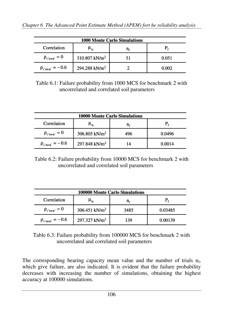
Chapter 6 The Advanced Point Estimate Method (APEM) fort he reliability analysis
106
0tan =ρϕ′′c
6.0tan −=ρϕ′′c
306.451 kN/m2
297.327 kN/m2
3485
139
0.03485
0.00139
100000 Monte Carlo Simulations
PfnffqµCorrelation
0tan =ρϕ′′c
6.0tan −=ρϕ′′c
306.451 kN/m2
297.327 kN/m2
3485
139
0.03485
0.00139
100000 Monte Carlo Simulations
PfnffqµCorrelation
0tan =ρϕ′′c
6.0tan −=ρϕ′′c
306.805 kN/m2
297.848 kN/m2
496
14
0.0496
0.0014
10000 Monte Carlo Simulations
PfnffqµCorrelation
0tan =ρϕ′′c
6.0tan −=ρϕ′′c
306.805 kN/m2
297.848 kN/m2
496
14
0.0496
0.0014
10000 Monte Carlo Simulations
PfnffqµCorrelation
Table 6.1: Failure probability from 1000 MCS for benchmark 2 with
uncorrelated and correlated soil parameters
Table 6.2: Failure probability from 10000 MCS for benchmark 2 with
uncorrelated and correlated soil parameters
Table 6.3: Failure probability from 100000 MCS for benchmark 2 with
uncorrelated and correlated soil parameters
The corresponding bearing capacity mean value and the number of trials nf,
which give failure, are also indicated. It is evident that the failure probability
decreases with increasing the number of simulations, obtaining the highest
accuracy at 100000 simulations.
0tan =ρϕ′′c
6.0tan −=ρϕ′′c
310.807 kN/m2
294.288 kN/m2
51
2
0.051
0.002
1000 Monte Carlo Simulations
PfnffqµCorrelation
0tan =ρϕ′′c
6.0tan −=ρϕ′′c
310.807 kN/m2
294.288 kN/m2
51
2
0.051
0.002
1000 Monte Carlo Simulations
PfnffqµCorrelation

6.2 Reliability analysis of the bearing capacity problem
107
Pf (1000 MCS)ϕ′′ρ tanc Pf (10000 MCS) Pf (100000 MCS)
0 0.051 0.0496 0.0348
-0.1 0.030 0.0371 0.0214
-0.2 0.021 0.0292 0.0169
-0.3 0.014 0.0194 0.0122
-0.4 0.005 0.0125 0.0078
-0.5 0.003 0.0056 0.0044
-0.6 0.002 0.0014 0.0014
-0.7 0 0.0001 0.0002
-0.8 0 0 0
-0.9 0 0 0
-1 0 0 0
Pf (1000 MCS)ϕ′′ρ tanc Pf (10000 MCS) Pf (100000 MCS)
0 0.051 0.0496 0.0348
-0.1 0.030 0.0371 0.0214
-0.2 0.021 0.0292 0.0169
-0.3 0.014 0.0194 0.0122
-0.4 0.005 0.0125 0.0078
-0.5 0.003 0.0056 0.0044
-0.6 0.002 0.0014 0.0014
-0.7 0 0.0001 0.0002
-0.8 0 0 0
-0.9 0 0 0
-1 0 0 0
To define the error referred to an estimated failure probability or, more
essentially, the number of Monte Carlo simulations necessary to obtain a certain
accuracy, the formula (6.3) after VRIJLING (1997) could be applied
f
f
PN
P1KE
⋅
−⋅= (6.3)
where Pf is the estimated failure probability, N is the required number of
simulations, K is the accuracy and E is the percent error associated with N.
Considering the failure probabilities of Table 6.2 for 10000 simulations with
ρc´tanϕ´ = 0 and ρc´tanϕ´ = -0.6, the corresponding percent error found applying
formula (6.3) with an accuracy of 95% will be, respectively, 4.2% and 25%. On
the other hand, formula (6.3) can also be used to evaluate the number of
simulations required for a higher accuracy. As an example, a percent error of
10% is desired to get the same failure probability of Table 6.2 for the case with a
negative correlation. Thus the number of simulations should be at least
N ≈64000.
Table 6.4 shows how the failure probability of the bearing capacity is
influenced by the correlation coefficient. These results show that much lower
probabilities of failure are found when the correlation coefficient between c´ and
tanϕ´ decreases from 0 to –1.0. In particular, for higher negative values of the
correlation coefficient the system is apparently safe with Pf = 0.
Table 6.4: Influence of the correlation coefficient on the failure probability for
benchmark 2

Chapter 6 The Advanced point Estimate Method (APEM) fort he reliability analysis
108
Fa
ilu
re
pro
ba
bil
ity
Pf
0.00
0.01
0.02
0.03
0.04
0.05
0.06
0 -0.1 -0.2 -0.3 -0.4 -0.5 -0.6 -0.7 -0.8 -0.9 -1
Correlation coefficient
1000 MCS 10000 MCS 100000 MCS
ϕ′′ρ tanc
Fa
ilu
re
pro
ba
bil
ity
Pf
0.00
0.01
0.02
0.03
0.04
0.05
0.06
0 -0.1 -0.2 -0.3 -0.4 -0.5 -0.6 -0.7 -0.8 -0.9 -1
Correlation coefficient
1000 MCS 10000 MCS 100000 MCS
ϕ′′ρ tanc
0tan =ρϕ′′c 6.0tan −=ρ
ϕ′′c
Failure probability of 10000 Monte Carlo Simulations
standard lognormal 0.0552 0.0031
shifted lognormal 0.0483 0.0013
assumed distribution 0tan =ρϕ′′c 6.0tan −=ρ
ϕ′′c
Failure probability of 10000 Monte Carlo Simulations
standard lognormal 0.0552 0.0031
shifted lognormal 0.0483 0.0013
assumed distribution
These facts are also shown in Fig. 6.1, where the failure probability is plotted
against the correlation coefficient of the soil strength parameters for different
Monte Carlo realisations.
If a certain density function is assumed as an approximation to plot MCS
results, as shown in Fig. 6.2, then different failure probabilities can be found.
Figure 6.1: Failure probability versus correlation coefficient for benchmark 2
Table 6.5: Failure probability of qf assuming a standard lognormal and a shifted
lognormal distribution as approximation of 10000 MCS with
ρc´tanϕ´ = 0 and ρc´tanϕ´ = -0.6
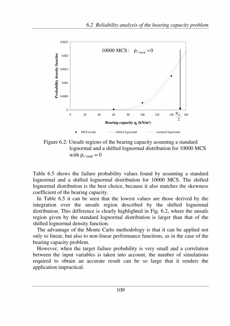
6.2 Reliability analysis of the bearing capacity problem
109
0
0.0005
0.001
0.0015
0.002
0.0025
0 20 40 60 80 100 120 140 160
Bearing capacity qf (kN/m^2)
Pro
ba
bil
ity
den
sity
fu
nct
ion
MCS results shifted lognormal standard lognormal
2
fqµ
0:10000 tan =ρϕ′′cMCS
Bearing capacity qf
(kN/m²)
0
0.0005
0.001
0.0015
0.002
0.0025
0 20 40 60 80 100 120 140 160
Bearing capacity qf (kN/m^2)
Pro
ba
bil
ity
den
sity
fu
nct
ion
MCS results shifted lognormal standard lognormal
2
fqµ
0:10000 tan =ρϕ′′cMCS
0
0.0005
0.001
0.0015
0.002
0.0025
0 20 40 60 80 100 120 140 160
Bearing capacity qf (kN/m^2)
Pro
ba
bil
ity
den
sity
fu
nct
ion
MCS results shifted lognormal standard lognormal
2
fqµ
0:10000 tan =ρϕ′′cMCS
Bearing capacity qf
(kN/m²)
Figure 6.2: Unsafe regions of the bearing capacity assuming a standard
lognormal and a shifted lognormal distribution for 10000 MCS
with ρc´tanϕ´ = 0
Table 6.5 shows the failure probability values found by assuming a standard
lognormal and a shifted lognormal distribution for 10000 MCS. The shifted
lognormal distribution is the best choice, because it also matches the skewness
coefficient of the bearing capacity.
In Table 6.5 it can be seen that the lowest values are those derived by the
integration over the unsafe region described by the shifted lognormal
distribution. This difference is clearly highlighted in Fig. 6.2, where the unsafe
region given by the standard lognormal distribution is larger than that of the
shifted lognormal density function.
The advantage of the Monte Carlo methodology is that it can be applied not
only to linear, but also to non-linear performance functions, as in the case of the
bearing capacity problem.
However, when the target failure probability is very small and a correlation
between the input variables is taken into account, the number of simulations
required to obtain an accurate result can be so large that it renders the
application impractical.
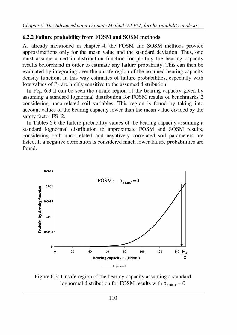
Chapter 6 The Advanced point Estimate Method (APEM) fort he reliability analysis
110
0
0.0005
0.001
0.0015
0.002
0.0025
0 20 40 60 80 100 120 140
Bearing capacity qf (kN7m^2)
Prob
ab
ilit
yd
en
sity
fun
cti
on
lognormal
2
fqµ
0: tan =ρϕ′′cFOSM
Bearing capacity qf
(kN/m²)
0
0.0005
0.001
0.0015
0.002
0.0025
0 20 40 60 80 100 120 140
Bearing capacity qf (kN7m^2)
Prob
ab
ilit
yd
en
sity
fun
cti
on
lognormal
2
fqµ
0: tan =ρϕ′′cFOSM
0
0.0005
0.001
0.0015
0.002
0.0025
0 20 40 60 80 100 120 140
Bearing capacity qf (kN7m^2)
Prob
ab
ilit
yd
en
sity
fun
cti
on
lognormal
2
fqµ
0: tan =ρϕ′′cFOSM
2
fqµ
0: tan =ρϕ′′cFOSM
Bearing capacity qf
(kN/m²)
6.2.2 Failure probability from FOSM and SOSM methods
As already mentioned in chapter 4, the FOSM and SOSM methods provide
approximations only for the mean value and the standard deviation. Thus, one
must assume a certain distribution function for plotting the bearing capacity
results beforehand in order to estimate any failure probability. This can then be
evaluated by integrating over the unsafe region of the assumed bearing capacity
density function. In this way estimates of failure probabilities, especially with
low values of Pf, are highly sensitive to the assumed distribution.
In Fig. 6.3 it can be seen the unsafe region of the bearing capacity given by
assuming a standard lognormal distribution for FOSM results of benchmarks 2
considering uncorrelated soil variables. This region is found by taking into
account values of the bearing capacity lower than the mean value divided by the
safety factor FS=2.
In Tables 6.6 the failure probability values of the bearing capacity assuming a
standard lognormal distribution to approximate FOSM and SOSM results,
considering both uncorrelated and negatively correlated soil parameters are
listed. If a negative correlation is considered much lower failure probabilities are
found.
Figure 6.3: Unsafe region of the bearing capacity assuming a standard
lognormal distribution for FOSM results with ρc´tanϕ´ = 0

6.2 Reliability analysis of the bearing capacity problem
111
When there is no information on the shape of the probability distribution, as in
the case of FOSM and SOSM methods, for which no skewness is provided,
another way of evaluating the reliability of the bearing capacity is to consider a
normal distribution and then calculate the reliability index, which only depends
on the first two moments of the performance function. Thus Eq. (2.24) can be
easily applied, considering the limit state function Z as
2qZ fq
f
µ−= (6.4)
where qf represents the resistance of the system, or ultimate bearing capacity, as
a random variable with a certain probability density function. While µqf/2 is the
deterministic load, given by the mean value of the bearing capacity divided by
the safety factor FS=2. For a more detailed description about the ultimate
bearing capacity and the corresponding safety factor the author refers to
Appendix A.
Instead of considering the load deterministically, it can also be considered as a
variable following a Dirac Delta function, given by
µ≠
µ=
=
2xif0
2xif1
)x(f
f
f
q
q
It has been shown that, when the soil parameters are negatively correlated, then
the failure probability is lower than when uncorrelated variables are considered.
Thus the reliability index is obviously higher, as this parameter is inversely
related to the failure probability.
However, if an appropriate form of the bearing capacity density function is
prescribed, the corresponding failure probability can be estimated by
transforming this function into an equivalent normal distribution using special
transformation formulas, such as the well-known Rosenblatt´s transformation
(ROSENBLATT, 1952).
Table 6.7 shows the reliability indeces of the bearing capacity by assuming a
standard lognormal distribution for FOSM and SOSM results for uncorrelated
soil parameters and for a negative correlation of –0.6. These values are obtained
using Eq. (2.25), valid for a standard lognormal distribution and considering the
limit state function Z as given by Eq. (6.4). The failure probability can then be

Chapter 6 The Advanced Point Estimate Method (APEM) for the reliability analysis
112
0.0516 0.0434
0.005 0.0043
lognormal distribution approximation
Correlation Pf(FOSM) Pf(SOSM)
0tan =ρϕ′′c
6.0tan −=ρϕ′′c
0.0516 0.0434
0.005 0.0043
lognormal distribution approximation
Correlation Pf(FOSM) Pf(SOSM)
0tan =ρϕ′′c
6.0tan −=ρϕ′′c
1.63 1.71
2.58 2.63
lognormal distribution approximation
Correlation (FOSM) (SOSM)
0tan =ρϕ′′c
6.0tan −=ρϕ′′c
β β
estimated by using Eq. (2.23). The results found are exactly those of Tables 6.6
and 6.7, thus confirming the failure probabilities estimated by integrating over
the unsafe region of the bearing capacity plotted in Fig. 6.3.
Table 6.6: Failure probability of qf assuming a standard lognormal distribution
for FOSM and SOSM results considering ρc´tanϕ´ = 0 and ρc´tanϕ´ = -0.6
Table 6.7: Reliability index of qf assuming a standard lognormal distribution for
FOSM and SOSM results considering ρc´tanϕ´ = 0 and ρc´tanϕ´ = -0.6
6.2.3 Failure probability from FORM
The First Order Reliability Method is also applied to evaluate the reliability of
the bearing capacity problem.
As already seen in chapter 3, an iterative solution is required for the FORM to
find the design point useful to identify the most probable combination of the
input variables at failure. This procedure can lead to time consuming
convergence problems when highly non-linear limit state functions are
considered. However for the bearing capacity problem the iterative process
converges rapidly, because only two input random variables are involved.

6.2 Reliability analysis of the bearing capacity problem
113
0tan =ρϕ′′c
6.0tan −=ρϕ′′c
β
Gaussian normal distribution approximation
0.0109
(FORM)
1.63
2.3
Correlation Pf(FORM)
0.0515
Table 6.8: Failure probability and reliability index of qf from VaP application,
assuming a normal distribution for FORM results with ρc´tanϕ´ = 0
and ρc´tanϕ´ = -0.6
For FORM application the soil cohesion, which is lognormally distributed,
needs to be transformed into a standard normal variable with zero mean and
standard deviation equal to unity, as, for example, described in VRIJLING
(1997). In this publication, the analytical “modus operandi” of the FORM is
reported. Results derived by the analytical procedure are then compared with
those of the numerical optimisation routine of the VaP 2.2 software, already
mentioned in chapter 3.
An advantage of the numerical method is that it offers the possibility to input
different correlation values directly in the form of a matrix, thus overcoming the
difficulties of the analytical procedure.
In addition, the level of accuracy of the VaP is very high. This is set at 10-6
.
This value can also be changed according to the accuracy required.
Because of the higher accuracy of the numerical procedure, only FORM
results derived by the VaP application are listed in Table 6.8. As the FORM
requires the transformation of a non-normal distribution into a Gaussian
distribution, the results are referred only to this function.
Compared to the case with ρc´tanϕ´ = 0, an almost 80% lower failure probability
and a 30% higher reliability index are found when a negative correlation of –0.6
between cohesion and friction angle is considered.
6.2.4 Failure probability from PEM
It should be pointed out again that, contrary to the FOSM and SOSM methods,
the PEM also provides the skewness coefficient of the bearing capacity.
This way it is possible to have an idea of the symmetry, or asymmetry, of the
bearing capacity density function.
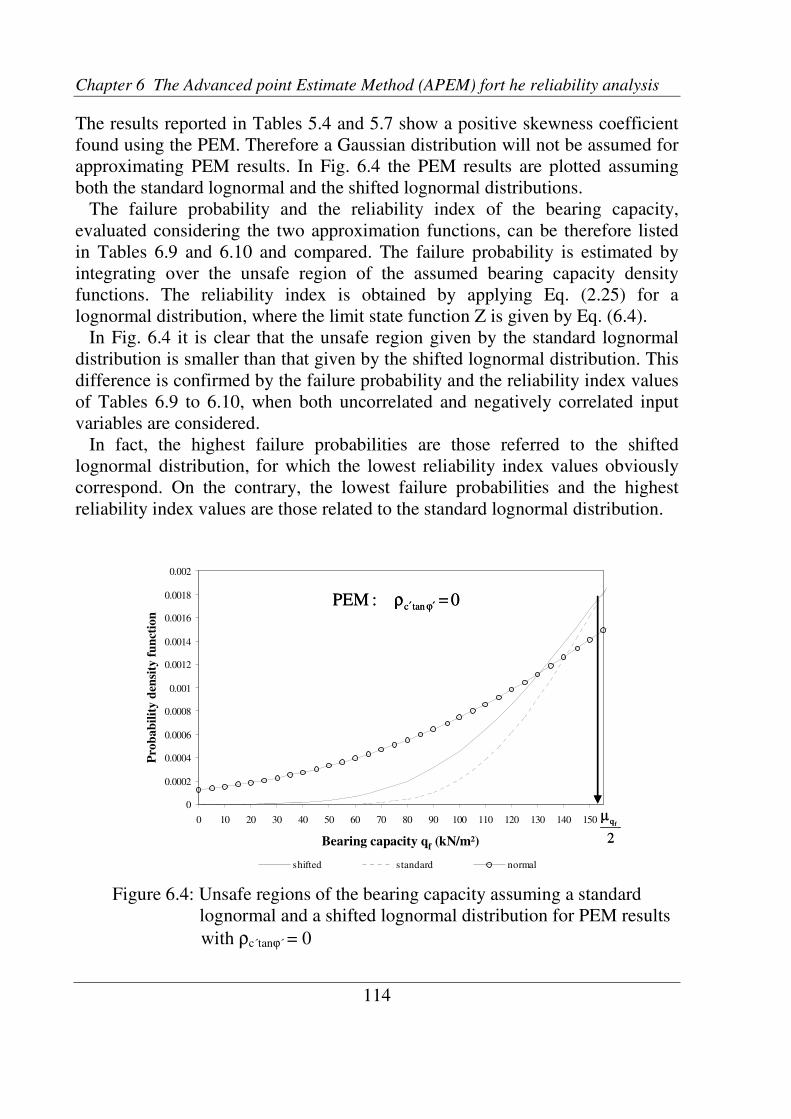
Chapter 6 The Advanced point Estimate Method (APEM) fort he reliability analysis
114
0
0.0002
0.0004
0.0006
0.0008
0.001
0.0012
0.0014
0.0016
0.0018
0.002
0 10 20 30 40 50 60 70 80 90 100 110 120 130 140 150
Bearing capacity qf (kN/m^2)
Pro
ba
bil
ity
den
sity
fu
nct
ion
shifted standard normal
0: tan =ρϕ′′cPEM
2
fqµ
Bearing capacity qf (kN/m²)
0
0.0002
0.0004
0.0006
0.0008
0.001
0.0012
0.0014
0.0016
0.0018
0.002
0 10 20 30 40 50 60 70 80 90 100 110 120 130 140 150
Bearing capacity qf (kN/m^2)
Pro
ba
bil
ity
den
sity
fu
nct
ion
shifted standard normal
0: tan =ρϕ′′cPEM
2
fqµ0
0.0002
0.0004
0.0006
0.0008
0.001
0.0012
0.0014
0.0016
0.0018
0.002
0 10 20 30 40 50 60 70 80 90 100 110 120 130 140 150
Bearing capacity qf (kN/m^2)
Pro
ba
bil
ity
den
sity
fu
nct
ion
shifted standard normal
0: tan =ρϕ′′cPEM
2
fqµ
0: tan =ρϕ′′cPEM
2
fqµ
Bearing capacity qf (kN/m²)
The results reported in Tables 5.4 and 5.7 show a positive skewness coefficient
found using the PEM. Therefore a Gaussian distribution will not be assumed for
approximating PEM results. In Fig. 6.4 the PEM results are plotted assuming
both the standard lognormal and the shifted lognormal distributions.
The failure probability and the reliability index of the bearing capacity,
evaluated considering the two approximation functions, can be therefore listed
in Tables 6.9 and 6.10 and compared. The failure probability is estimated by
integrating over the unsafe region of the assumed bearing capacity density
functions. The reliability index is obtained by applying Eq. (2.25) for a
lognormal distribution, where the limit state function Z is given by Eq. (6.4).
In Fig. 6.4 it is clear that the unsafe region given by the standard lognormal
distribution is smaller than that given by the shifted lognormal distribution. This
difference is confirmed by the failure probability and the reliability index values
of Tables 6.9 to 6.10, when both uncorrelated and negatively correlated input
variables are considered.
In fact, the highest failure probabilities are those referred to the shifted
lognormal distribution, for which the lowest reliability index values obviously
correspond. On the contrary, the lowest failure probabilities and the highest
reliability index values are those related to the standard lognormal distribution.
Figure 6.4: Unsafe regions of the bearing capacity assuming a standard
lognormal and a shifted lognormal distribution for PEM results
with ρc´tanϕ´ = 0

6.2 Reliability analysis of the bearing capacity problem
115
0tan =ρϕ′′c
6.0tan −=ρϕ′′c
β
standard lognormal distribution approximation
Correlation Pf(PEM) (PEM)
0.0484 1.66
0.0052 2.56
0tan =ρϕ′′c
6.0tan −=ρϕ′′c
β
standard lognormal distribution approximation
Correlation Pf(PEM) (PEM)
0.0484 1.66
0.0052 2.56
0tan =ρϕ′′c
6.0tan −=ρϕ′′c
β
shifted lognormal distribution approximation
Correlation Pf(PEM) (PEM)
0.0651 1.56
0.0185 2.27
0tan =ρϕ′′c
6.0tan −=ρϕ′′c
β
shifted lognormal distribution approximation
Correlation Pf(PEM) (PEM)
0.0651 1.56
0.0185 2.27
Table 6.9: Failure probability and reliability index of qf assuming a standard
lognormal distribution for PEM results considering ρc´tanϕ´ = 0 and
ρc´tanϕ´ = -0.6
Table 6.10: Failure probability and reliability index of qf assuming a shifted
lognormal distribution for PEM results considering ρc´tanϕ´ = 0 and
ρc´tanϕ´ = -0.6
6.2.5 Comparison of failure probabilities and necessity of a new approach
The aim of this section is to compare the failure probabilities of the bearing
capacity previously estimated using Monte Carlo, PEM, FORM, FOSM and
SOSM methods.
It is important to stress again that the MCS results do not need to be
approximated by a certain probability density function, because this method
already provides both the shape of the distribution curve and the failure
probability for the bearing capacity problem. However different probability
functions are considered here to show that one of these curves can more
effectively approximate the results of the probabilistic methods applied.
Chapter 6 The Advanced point Estimate Method (APEM) fort he reliability analysis
116
The bearing capacity values representing the right extremes of the unsafe
regions of the assumed probability density function, for which the target failure
probability should be evaluated are listed in Table 6.11. As already mentioned,
these values are estimated by dividing the bearing capacity mean values, found
by applying different probabilistic methods, by a safety factor of 2. They are all
very similar. The PEM values, however, are closer to those of MCS. Of course
FOSM and FORM values are exactly the same, because they are found by
applying the same formula, being the FORM an enhancement of FOSM.
Nevertheless, different right extreme values could be chosen to evaluate the
failure probability, depending on the reliability level that one wants to achieve
for the bearing capacity problem. In this section, only the values listed in Table
6.11 are taken into account.
The values 200 kN/m2
and 250 kN/m2 will be further considered for evaluating
the failure probability of the bearing capacity by applying the advanced PEM.
For more details, the author refers to section 6.3.
The unsafe regions found considering the right extremes of Table 6.11 and
assuming a Gaussian normal, a standard lognormal and a shifted lognormal
distribution as approximations of the bearing capacity results are plotted in Figs.
6.5, 6.6 and 6.7. These diagrams are drawn for both uncorrelated and negatively
correlated soil parameters.
In particular, in Figs. 6.5 and 6.6 the unsafe regions referred to the results
derived from all the probabilistic methods analysed, except for the FORM, are
shown. The iterative procedure of the FORM method does not provide proper
mean values and standard deviations of the bearing capacity (i.e. they vary
depending on the choice of the design point), which can be compared with the
statistical values of other methods. Nevertheless it gives the failure probability
and the reliability index. In Fig. 6.7 only the MCS and PEM results are
considered in the plot of the unsafe regions of the bearing capacity by assuming
a shifted lognormal function. This is because the FOSM, SOSM and FORM
methods do not provide any skewness values.
From these diagrams it is possible to see how the unsafe region decreases
when a negative correlation is taking into account, especially for the MCS
results approximated by a shifted lognormal distribution in Fig. 6.7.
This fact is more clear when Tables 6.12, 6.13 and 6.14 are examined. Here
the failure probability evaluated by considering all probabilistic approaches and
all assumed probability distributions are shown.
The analysis of the values of Tables 6.12, 6.13 and 6.14 illustrates, first of all,
the importance of the correlation coefficient between c´ and tanϕ´ with respect
to the failure probability (or conversely to the reliability index).

6.2 Reliability analysis of the bearing capacity problem
117
0tan =ρϕ′′c
6.0tan −=ρϕ′′c
fqµ
151.925 145.439
148.924 149.627 145.439 148.033 145.439
153.403 153.393 145.439
bearing capacity mean value (kN/m2) / safety factor FS=2
Correlation 10000 MCS PEM FOSM SOSM FORM
0tan =ρϕ′′c
6.0tan −=ρϕ′′c
fqµ
151.925 145.439
148.924 149.627 145.439 148.033 145.439
153.403 153.393 145.439
bearing capacity mean value (kN/m2) / safety factor FS=2
Correlation 10000 MCS PEM FOSM SOSM FORM
0
0.0002
0.0004
0.0006
0.0008
0.001
0.0012
0.0014
0.0016
0.0018
0.002
0 20 40 60 80 100 120 140 160
Bearing capacity qf (kN/m^2)
Pro
ba
bil
ity
den
sity
fu
nct
ion
MCS PEM FOSM SOSM
0
0.0002
0.0004
0.0006
0.0008
0.001
0.0012
0 20 40 60 80 100 120 140 160
Bearing capacity qf (kN/m^2)
Pro
bab
ilit
y d
ensi
ty f
un
ctio
n
MCS PEM FOSM SOSM
0tan =ρϕ′′c
6.0tan −=ρϕ′′c
0
0.0002
0.0004
0.0006
0.0008
0.001
0.0012
0.0014
0.0016
0.0018
0.002
0 20 40 60 80 100 120 140 160
Bearing capacity qf (kN/m^2)
Pro
ba
bil
ity
den
sity
fu
nct
ion
MCS PEM FOSM SOSM
0
0.0002
0.0004
0.0006
0.0008
0.001
0.0012
0 20 40 60 80 100 120 140 160
Bearing capacity qf (kN/m^2)
Pro
bab
ilit
y d
ensi
ty f
un
ctio
n
MCS PEM FOSM SOSM
0tan =ρϕ′′c
6.0tan −=ρϕ′′c
Bearing capacity qf (kN/m²) Bearing capacity qf (kN/m²)
0
0.0002
0.0004
0.0006
0.0008
0.001
0.0012
0.0014
0.0016
0.0018
0.002
0 20 40 60 80 100 120 140 160
Bearing capacity qf (kN/m^2)
Pro
ba
bil
ity
den
sity
fu
nct
ion
MCS PEM FOSM SOSM
0
0.0002
0.0004
0.0006
0.0008
0.001
0.0012
0 20 40 60 80 100 120 140 160
Bearing capacity qf (kN/m^2)
Pro
bab
ilit
y d
ensi
ty f
un
ctio
n
MCS PEM FOSM SOSM
0tan =ρϕ′′c
6.0tan −=ρϕ′′c
0
0.0002
0.0004
0.0006
0.0008
0.001
0.0012
0.0014
0.0016
0.0018
0.002
0 20 40 60 80 100 120 140 160
Bearing capacity qf (kN/m^2)
Pro
ba
bil
ity
den
sity
fu
nct
ion
MCS PEM FOSM SOSM
0
0.0002
0.0004
0.0006
0.0008
0.001
0.0012
0 20 40 60 80 100 120 140 160
Bearing capacity qf (kN/m^2)
Pro
bab
ilit
y d
ensi
ty f
un
ctio
n
MCS PEM FOSM SOSM
0tan =ρϕ′′c
6.0tan −=ρϕ′′c
Bearing capacity qf (kN/m²) Bearing capacity qf (kN/m²)
In fact when a negative correlation is considered in the calculation very different
values of Pf, compared to the case with ρc´tanϕ´ = 0, are obtained, which are lower
when ρc´tanϕ´ = -0.6. In other words, if the correlation is not considered, then the
failure probabilities are higher than those actually observed when a negative
correlation is imposed.
The real failure probabilities found by applying 10000 Monte Carlo
simulations are those of Table 6.2. The fictitious failure probabilities in the
hypothesis of assuming a certain probability distribution for the bearing capacity
results of MCS are listed in Tables 6.12, 6.13 and 6.14.
An idea of the accuracy given by assuming different probability density
functions when compared to the real values of the failure probability found by
MCS is given in Table 6.15.
Table 6.11: Right extreme values of the bearing capacity unsafe regions for
which the failure probability is evaluated
Figure 6.5: Unsafe regions of qf assuming a normal distribution for different
probabilistic methods considering ρc´tanϕ´ = 0 and ρc´tanϕ´ = -0.6

Chapter 6 The Advanced Point Estimate Method (APEM) for the reliability analysis
118
0
0.0002
0.0004
0.0006
0.0008
0.001
0.0012
0 20 40 60 80 100 120 140 160
Bearing capacity qf (kN/m^2)
Prob
ab
ilit
y d
en
sity
fu
ncti
on
MCS PEM FOSM SOSM
0
0.0005
0.001
0.0015
0.002
0.0025
0 20 40 60 80 100 120 140 160
Bearing capacity qf (kN/m^2)
Pro
ba
bil
ity
den
sity
fu
nct
ion
MCS PEM FOSM SOSM
0tan =ρϕ′′c
6.0tan −=ρϕ′′c
0
0.0002
0.0004
0.0006
0.0008
0.001
0.0012
0 20 40 60 80 100 120 140 160
Bearing capacity qf (kN/m^2)
Prob
ab
ilit
y d
en
sity
fu
ncti
on
MCS PEM FOSM SOSM
0
0.0005
0.001
0.0015
0.002
0.0025
0 20 40 60 80 100 120 140 160
Bearing capacity qf (kN/m^2)
Pro
ba
bil
ity
den
sity
fu
nct
ion
MCS PEM FOSM SOSM
0tan =ρϕ′′c
6.0tan −=ρϕ′′c
Bearing capacity qf (kN/m²) Bearing capacity qf (kN/m²)
0
0.0002
0.0004
0.0006
0.0008
0.001
0.0012
0 20 40 60 80 100 120 140 160
Bearing capacity qf (kN/m^2)
Prob
ab
ilit
y d
en
sity
fu
ncti
on
MCS PEM FOSM SOSM
0
0.0005
0.001
0.0015
0.002
0.0025
0 20 40 60 80 100 120 140 160
Bearing capacity qf (kN/m^2)
Pro
ba
bil
ity
den
sity
fu
nct
ion
MCS PEM FOSM SOSM
0tan =ρϕ′′c
6.0tan −=ρϕ′′c
0
0.0002
0.0004
0.0006
0.0008
0.001
0.0012
0 20 40 60 80 100 120 140 160
Bearing capacity qf (kN/m^2)
Prob
ab
ilit
y d
en
sity
fu
ncti
on
MCS PEM FOSM SOSM
0
0.0005
0.001
0.0015
0.002
0.0025
0 20 40 60 80 100 120 140 160
Bearing capacity qf (kN/m^2)
Pro
ba
bil
ity
den
sity
fu
nct
ion
MCS PEM FOSM SOSM
0tan =ρϕ′′c
6.0tan −=ρϕ′′c
Bearing capacity qf (kN/m²) Bearing capacity qf (kN/m²)
0
0.0002
0.0004
0.0006
0.0008
0.001
0.0012
0 20 40 60 80 100 120 140 160
Bearing capacity qf (kN/m^2)
Pro
ba
bil
ity
den
sity
fu
nct
ion
MCS PEM
0
0.0005
0.001
0.0015
0.002
0.0025
0 20 40 60 80 100 120 140 160
Bearing capacity qf (kN/m^2)
Pro
ba
bil
ity
den
sity
fu
nct
ion
MCS PEM
0tan =ρϕ′′c
6.0tan −=ρϕ′′c
0
0.0002
0.0004
0.0006
0.0008
0.001
0.0012
0 20 40 60 80 100 120 140 160
Bearing capacity qf (kN/m^2)
Pro
ba
bil
ity
den
sity
fu
nct
ion
MCS PEM
0
0.0005
0.001
0.0015
0.002
0.0025
0 20 40 60 80 100 120 140 160
Bearing capacity qf (kN/m^2)
Pro
ba
bil
ity
den
sity
fu
nct
ion
MCS PEM
0tan =ρϕ′′c
6.0tan −=ρϕ′′c
Bearing capacity qf (kN/m²)Bearing capacity qf (kN/m²)
0
0.0002
0.0004
0.0006
0.0008
0.001
0.0012
0 20 40 60 80 100 120 140 160
Bearing capacity qf (kN/m^2)
Pro
ba
bil
ity
den
sity
fu
nct
ion
MCS PEM
0
0.0005
0.001
0.0015
0.002
0.0025
0 20 40 60 80 100 120 140 160
Bearing capacity qf (kN/m^2)
Pro
ba
bil
ity
den
sity
fu
nct
ion
MCS PEM
0tan =ρϕ′′c
6.0tan −=ρϕ′′c
0
0.0002
0.0004
0.0006
0.0008
0.001
0.0012
0 20 40 60 80 100 120 140 160
Bearing capacity qf (kN/m^2)
Pro
ba
bil
ity
den
sity
fu
nct
ion
MCS PEM
0
0.0005
0.001
0.0015
0.002
0.0025
0 20 40 60 80 100 120 140 160
Bearing capacity qf (kN/m^2)
Pro
ba
bil
ity
den
sity
fu
nct
ion
MCS PEM
0tan =ρϕ′′c
6.0tan −=ρϕ′′c
Bearing capacity qf (kN/m²)Bearing capacity qf (kN/m²)
From this Table, it is clear that the fictitious failure probabilities found by
assuming a shifted lognormal distribution are more accurate than when a normal
and a standard lognormal distributions are considered. This is an additional good
reason for choosing the shifted lognormal distribution as an approximation of
the bearing capacity results. In fact, the fictitious failure probability of MCS
increases greatly when a Gaussian distribution is taken into account, thus
showing how a probabilistic result can deviate from reality depending on the
assumption considered.
Figure 6.6: Unsafe regions of qf assuming a standard lognormal distribution for
different probabilistic methods considering ρc´tanϕ´ = 0 and
ρc´tanϕ´ = -0.6
Figure 6.7: Unsafe regions of qf assuming a shifted lognormal distribution for
different probabilistic methods considering ρc´tanϕ´ = 0 and
ρc´tanϕ´ = -0.6

6.2 Reliability analysis of the bearing capacity problem
119
0tan =ρϕ′′c
6.0tan −=ρϕ′′c 0.0254 0.0109
SOSM FORM
0.1029 0.0931 0.0515
FOSM
0.0275
0.1005* 0.0936
0.0212* 0.0308
Correlation 10000 MCS PEM
Failure probability by assuming a Gaussian normal distribution
* fictit ious value. The rea l M CS failure probabilities are reported in Tab le 6.2.
0tan =ρϕ′′c
6.0tan −=ρϕ′′c 0.0254 0.0109
SOSM FORM
0.1029 0.0931 0.0515
FOSM
0.0275
0.1005* 0.0936
0.0212* 0.0308
Correlation 10000 MCS PEM
Failure probability by assuming a Gaussian normal distribution
* fictit ious value. The rea l M CS failure probabilities are reported in Tab le 6.2.
0tan =ρϕ′′c
6.0tan −=ρϕ′′c
0.0552*
FORM
0.0434 -
0.0031* 0.0052 0.005 0.0043 -
0.0484 0.0516
Failure probability by assuming a standard lognormal distribution
Correlation 10000 MCS PEM FOSM SOSM
* fictit ious value. The rea l M CS failure probabilities are reported in Tab le 6.2.
0tan =ρϕ′′c
6.0tan −=ρϕ′′c
0.0552*
FORM
0.0434 -
0.0031* 0.0052 0.005 0.0043 -
0.0484 0.0516
Failure probability by assuming a standard lognormal distribution
Correlation 10000 MCS PEM FOSM SOSM
* fictit ious value. The rea l M CS failure probabilities are reported in Tab le 6.2.
A comparison of the FORM results of Table 6.12 with the MCS failure
probabilities reported in Table 6.2 shows that the FORM method, based on the
assumption of normal input variables, gives higher values than MCS. Two main
causes of this discrepancy are: firstly, the bearing capacity is highly non-linear
with tanϕ´, which is one of the input variables that play an important role in this
analysis. In fact, it is well-known that a linear approximation in the FORM
design point causes some serious error in the estimation of the reliability index,
thus influencing also the value of the failure probability. Secondly, the input
variable cohesion follows a distribution, which is far from the normal
distribution, thus introducing additional uncertainties in the final results when
this is transformed to a normal variable.
Table 6.12: Failure probability of qf assuming a normal distribution for different
probabilistic methods considering ρc´tanϕ´ = 0 and ρc´tanϕ´ = -0.6
Table 6.13: Failure probability of qf assuming a standard lognormal distribution
for different probabilistic methods considering ρc´tanϕ´ = 0 and
ρc´tanϕ´ = -0.6

Chapter 6 The Advanced point Estimate Method (APEM) fort he reliability analysis
120
0tan =ρϕ′′c
6.0tan −=ρϕ′′c
- -
0.0013* 0.0185 - - -
0.0483* 0.0651 -
Failure probability by assuming a shifted lognormal distribution
Correlation 10000 MCS PEM FOSM SOSM FORM
* fictit ious value. The rea l M CS failure probabilities are reported in Tab le 6.2.
0tan =ρϕ′′c
6.0tan −=ρϕ′′c
- -
0.0013* 0.0185 - - -
0.0483* 0.0651 -
Failure probability by assuming a shifted lognormal distribution
Correlation 10000 MCS PEM FOSM SOSM FORM
* fictit ious value. The rea l M CS failure probabilities are reported in Tab le 6.2.
0tan =ρϕ′′c 6.0tan −=ρ
ϕ′′c
Accuracy [%] of MCS results assuming different PDFs
standard lognormal
50%
shifted lognormal
assumed PDF
normal 10%
90% 45%
97% 93%
0tan =ρϕ′′c 6.0tan −=ρ
ϕ′′c
Accuracy [%] of MCS results assuming different PDFs
standard lognormal
50%
shifted lognormal
assumed PDF
normal 10%
90% 45%
97% 93%
Table 6.14: Failure probability of qf assuming a shifted lognormal distribution
for different probabilistic methods considering ρc´tanϕ´ = 0 and
ρc´tanϕ´ = -0.6
Table 6.15: Accuracy of the failure probability values found by assuming a
normal, a standard lognormal and a shifted lognormal
distribution to approximate MCS results
One should therefore be very careful in applying the approximation procedure of
FORM in the reliability analysis of a structure that has a highly non-linear
performance function, such as a shallow foundation design. This fact is also
valid for FOSM and SOSM methods, as already stressed in chapter 3.
When a standard lognormal distribution is considered, it seems to be that the
failure probabilities evaluated using the PEM are apparently closer to MCS
values of Table 6.2, especially for the case with uncorrelated soil parameters.
However, it has been previously shown that the shifted lognormal distribution
approximates MCS results best. Then only the failure probabilities referred to
6.3 Application of the Advanced PEM to the bearing capacity problem
121
this function should be taken into account. These values are listed in Table 6.14,
where PEM failure probabilities are given together with the fictitious ones of
MCS. The PEM, as a direct non-iterative method, overcomes the convergence
problem of FORM, thus being a more promising alternative. Unfortunately, in
this case the PEM results are even higher than those of FORM method, when
compared with the real failure probability values of MCS, shown in Table 6.2.
In order to cope with the shortcoming of the PEM in evaluating low failure
probabilities, a new method is proposed, referred to as the advanced PEM. The
methodology of the proposed approach is described in detail in the next section.
6.3 Application of the Advanced PEM to the bearing capacity problem
In the previous section the necessity of developing a new probabilistic method is
stated. The aim of this section is to describe this new methodology, called
Advanced Point Estimate Method, or shortly APEM, which is not yet available
in the literature, and to show its application to the bearing capacity problem.
6.3.1 Short description of the Advanced PEM methodology
The basic idea of the Advanced PEM is to focus on the critical values of the
input data, i.e. cohesion and friction angle, which could cause bearing capacity
failure. The reduced intervals of the soil parameters can be found using an
iteration procedure or by experts opinion.
Then the PEM is applied to these reduced intervals and the bearing capacity
statistical values are plotted in a graph by assuming the well-known shifted
lognormal distribution. It is then possible to evaluate low failure probabilities of
the bearing capacity more precisely. These values are then compared with the
Monte Carlo failure probabilities of Table 6.2 to verify the accuracy of the
APEM.
6.3.2 The reduced intervals of the input soil parameters
In chapter 4 it has been seen that the effective soil cohesion and friction angle
are described respectively by a standard lognormal and a normal distribution
with their corresponding statistical values, as shown in Figs. 4.1(a), (b) and 4.2.
For the new probabilistic method, i.e. the APEM, a reduced interval of both
parameters should be considered. These intervals contain values of the cohesion
and friction angle, which can most probably cause bearing capacity failure.

Chapter 6 The Advanced point Estimate Method (APEM) fort he reliability analysis
122
0
0.05
0.1
0.15
0.2
0.25
0.01 0.5 1 1.5 2 2.5 3
Cohesion c´ (kN/m^2)
Pro
ba
bil
ity
den
sity
fu
nct
ion
0
0.5
1
1.5
2
2.5
0.2 0.23 0.26 0.29 0.32 0.35 0.38
tan (°)
Pro
ba
bil
ity
den
sity
fu
nct
ion
ϕ′(kN/m²)
0
0.05
0.1
0.15
0.2
0.25
0.01 0.5 1 1.5 2 2.5 3
Cohesion c´ (kN/m^2)
Pro
ba
bil
ity
den
sity
fu
nct
ion
0
0.5
1
1.5
2
2.5
0.2 0.23 0.26 0.29 0.32 0.35 0.38
tan (°)
Pro
ba
bil
ity
den
sity
fu
nct
ion
ϕ′(kN/m²)
Figure 6.8: Reduced intervals of the soil input variables
There are two different ways of establishing these ranges, either by choosing
them on the basis of experts knowledge or using an iteration procedure:
- “experts” are geotechnical engineers who know the behaviour of the soil
layer in question, thus being able to better judge which values of the shear
parameters can be more dangerous for the stability of the strip footing
considered;
- the iteration procedure can be represented by an algorithm which considers
different combinations of soil cohesion and friction angle values and finding
those which give failure of the bearing capacity problem.
For this study an algorithm, described in appendix C, has been implemented in
MATLAB®
Version7.0 to determine the reduced intervals of the soil parameters
c´ and tanϕ´.
It has been observed that the cohesion has a negligible influence on the
bearing capacity compared to the friction angle. For this reason a constant range
of 0 - 3 kN/m2 is considered for this soil parameter. While for the friction angle
the algorithm finds a value of 21°, i.e. tanϕ´≈0.384, if the right extreme value of
the unsafe region of the bearing capacity is considered to be equal to its mean
value divided by a safety factor 2. The reduced intervals are then plotted in Fig.
6.8. The corresponding statistical values are respectively
- for c´: 08.0;m/kN65.0;m/kN87.1redc
2
redc
2
redc−=ν=σ=µ
′′′
- for tanϕ´: 37.1;02.0;35.0redtanredtanredtan
−=ν=σ=µϕ′ϕ′ϕ′
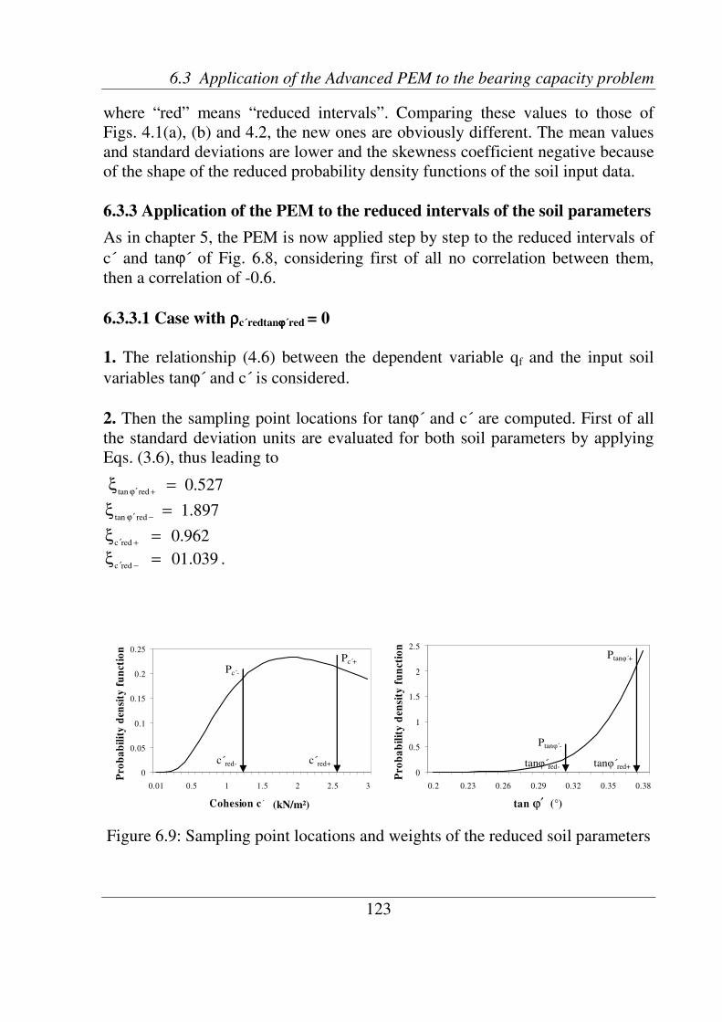
6.3 Application of the Advanced PEM to the bearing capacity problem
123
0
0.05
0.1
0.15
0.2
0.25
0.01 0.5 1 1.5 2 2.5 3
Cohesion c´ (kN/m^2)
Pro
ba
bil
ity
den
sity
fu
nct
ion
0
0.5
1
1.5
2
2.5
0.2 0.23 0.26 0.29 0.32 0.35 0.38
tan (°)
Pro
ba
bil
ity
den
sity
fu
nct
ion
ϕ′
c´red+c´red-
Pc´+
Pc -
tanφ red- tanφ red+
Ptanφ -
Ptanφ´+
(kN/m²)
0
0.05
0.1
0.15
0.2
0.25
0.01 0.5 1 1.5 2 2.5 3
Cohesion c´ (kN/m^2)
Pro
ba
bil
ity
den
sity
fu
nct
ion
0
0.5
1
1.5
2
2.5
0.2 0.23 0.26 0.29 0.32 0.35 0.38
tan (°)
Pro
ba
bil
ity
den
sity
fu
nct
ion
ϕ′
c´red+c´red-
Pc´+
Pc -
tanφ red- tanφ red+
Ptanφ -
Ptanφ´+
(kN/m²)
where “red” means “reduced intervals”. Comparing these values to those of
Figs. 4.1(a), (b) and 4.2, the new ones are obviously different. The mean values
and standard deviations are lower and the skewness coefficient negative because
of the shape of the reduced probability density functions of the soil input data.
6.3.3 Application of the PEM to the reduced intervals of the soil parameters
As in chapter 5, the PEM is now applied step by step to the reduced intervals of
c´ and tanϕ´ of Fig. 6.8, considering first of all no correlation between them,
then a correlation of -0.6.
6.3.3.1 Case with ρρρρc´redtanϕϕϕϕ´red = 0
1. The relationship (4.6) between the dependent variable qf and the input soil
variables tanϕ´ and c´ is considered.
2. Then the sampling point locations for tanϕ´ and c´ are computed. First of all
the standard deviation units are evaluated for both soil parameters by applying
Eqs. (3.6), thus leading to
527.0redtan
=ξ+ϕ′
897.1redtan
=ξ−ϕ′
962.0redc
=ξ+′
039.01redc
=ξ−′
.
Figure 6.9: Sampling point locations and weights of the reduced soil parameters

Chapter 6 The Advanced Point Estimate Method (APEM) for the reliability analysis
124
Hence the corresponding sampling point locations can be evaluated using Eqs.
(3.7), which give
309.0redtan =ϕ′−
368.0redtan =ϕ′+
2
m/kN503.2red´c =+
2
m/kN192.1red´c =−
.
3. The weights Pi, giving each of the four point estimates of soil parameters
considered as single random variables, are then determined using Eq. (3.8) valid
for a single random variable,
782.0Predtan
=+ϕ′
217.0Predtan
=−ϕ′
519.0Predc
=+′
481.0Predc
=−′
.
Figure 6.9 shows the locations of the sampling points of both soil parameters
tanϕ´ and c´. The corresponding weights are also shown in this diagram. Then
the associated weights need to be found, considering the input parameters as
multiple uncorrelated variables. For this aim Eq. (3.13) is here applied, which
gives the following values
406.0PPPredcredtan
=⋅=+′+ϕ′++
376.0PPPredcredtan
=⋅=−′+ϕ′−+
113.0PPPredcredtan
=⋅=+′−ϕ′+−
105.0PPPredcredtan
=⋅=−′−ϕ′−−
.
4. The value of the bearing capacity at each sampling point can then be
evaluated. The results are shown in Table 6.16.

6.3 Application of the Advanced PEM to the bearing capacity problem
125
-0.823130.641 kN/m2
19.278 kN/m2 0.148
fqµfqσ
fqCOVfqν
-0.823130.641 kN/m2
19.278 kN/m2 0.148
fqµfqσ
fqCOVfqν
±±P
±ϕ′tan
±±fq±′c
2.503 kN/m2 0.309 106.494 kN/m
2
0.105 1.192 kN/m2 0.309 90.153 kN/m
2
0.406
0.376
0.113
2.503 kN/m2 0.368 148.705 kN/m
2
1.192 kN/m2 0.368 129.004 kN/m
2
±±P
±ϕ′tan
±±fq±′c
2.503 kN/m2 0.309 106.494 kN/m
2
0.105 1.192 kN/m2 0.309 90.153 kN/m
2
0.406
0.376
0.113
2.503 kN/m2 0.368 148.705 kN/m
2
1.192 kN/m2 0.368 129.004 kN/m
2
2.503 kN/m2 0.309 106.494 kN/m
2
0.105 1.192 kN/m2 0.309 90.153 kN/m
2
0.406
0.376
0.113
2.503 kN/m2 0.368 148.705 kN/m
2
1.192 kN/m2 0.368 129.004 kN/m
2
Table 6.16: Associated weights, sampling points and bearing capacity values for
the reduced intervals of tanϕ´ and c´
5. Now the mean value, variance and skewness coefficient of the bearing
capacity can be determined using Eqs. (3.15), (3.16) and (3.17), where n = 2.
The results of the statistical estimates of qf predicted by PEM considering small
values of the input soil parameters are presented in Table 6.17.
Table 6.17: Statistical values of qf predicted by PEM considering reduced
intervals of the uncorrelated soil parameters
The bearing capacity results reported in Tables 6.16 and 6.17 are clearly lower
than those of Tables 5.3 and 5.4, due to the consideration of smaller values of
the cohesion and friction angle. In addition, the skewness coefficient is negative,
thus the probability density function of the bearing capacity should be
negatively skewed. This distribution should be at the same time able to
approximate the statistical results of Table 6.17 best and to give a failure
probability similar to the MCS value of Table 6.2 for uncorrelated soil
parameters.

Chapter 6 The Advanced point Estimate Method (APEM) fort he reliability analysis
126
±±P
±ϕ′tan ±±fq
±′c
0.163 2.503 kN/m2 0.368 148.956 kN/m
2
0.602 1.192 kN/m2 0.368 129.244 kN/m
2
0.181 2.503 kN/m2 0.309 106.695 kN/m
2
0.042 1.192 kN/m2 0.309 90.342 kN/m
2
±±P
±ϕ′tan ±±fq
±′c
0.163 2.503 kN/m2 0.368 148.956 kN/m
2
0.602 1.192 kN/m2 0.368 129.244 kN/m
2
0.181 2.503 kN/m2 0.309 106.695 kN/m
2
0.042 1.192 kN/m2 0.309 90.342 kN/m
2
0.163 2.503 kN/m2 0.368 148.956 kN/m
2
0.602 1.192 kN/m2 0.368 129.244 kN/m
2
0.181 2.503 kN/m2 0.309 106.695 kN/m
2
0.042 1.192 kN/m2 0.309 90.342 kN/m
2
The reason of choosing this particular density function the author refers to
section 6.3.4, where a shifted lognormal distribution will be assumed to
approximate the reduced bearing capacity results.
6.3.3.2 Case with ρρρρc´redtanϕϕϕϕ´red = -0.6
When negatively correlated soil parameters are considered then the steps 1 to 3
lead to the same results as the case with uncorrelated soil parameters. The only
difference is that the associated weights change because of the contribution of
the correlation coefficient –0.6. The formula of Christian (3.13) can be easily
applied here, thus giving
( ) 163.06.01PPPredcredtan
=−⋅⋅=+′+ϕ′++
( ) 602.06.01PPPredcredtan
=+⋅⋅=−′+ϕ′−+
( ) 181.06.01PPPredcredtan
=+⋅⋅=+′−ϕ′+−
( ) 042.06.01PPPredcredtan
=−⋅⋅=−′−ϕ′−−
.
4. The values of the bearing capacity at each sampling point are reported in
Table 6.18.
Table 6.18: Associated weights, sampling points and bearing capacity values for
the reduced intervals of tanϕ´ and c´ with ρc´redtanϕ´red = -0.6
5. Now the statistical values of the bearing capacity can be determined using
Eqs. (3.15), (3.16) and (3.17), where n = 2. Then the results predicted by PEM
considering small values of the input soil parameters are shown in Table 6.19.
The bearing capacity mean value and standard deviation reported in Tables
6.19 are slightly lower than those of Table 6.17, due to the consideration of a
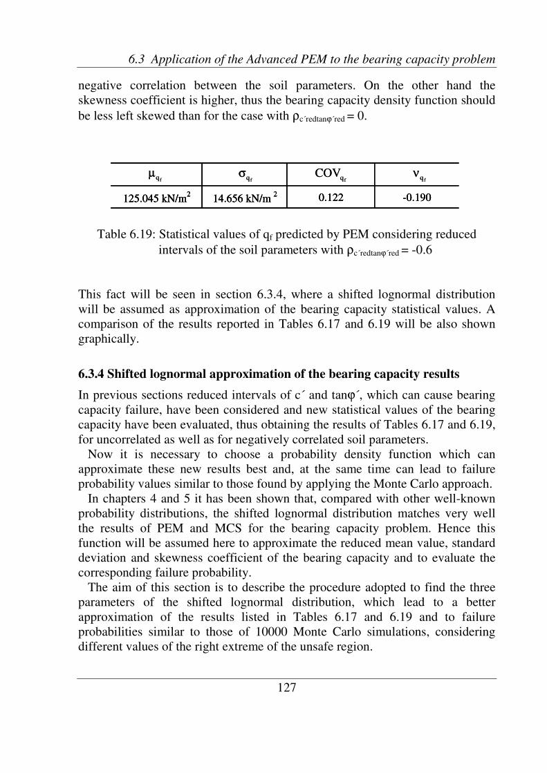
6.3 Application of the Advanced PEM to the bearing capacity problem
127
fqµfqσ
fqCOVfqν
125.045 kN/m2
14.656 kN/m2 0.122 -0.190
fqµfqσ
fqCOVfqν
125.045 kN/m2
14.656 kN/m2 0.122 -0.190125.045 kN/m
214.656 kN/m
2 0.122 -0.190
negative correlation between the soil parameters. On the other hand the
skewness coefficient is higher, thus the bearing capacity density function should
be less left skewed than for the case with ρc´redtanϕ´red = 0.
Table 6.19: Statistical values of qf predicted by PEM considering reduced
intervals of the soil parameters with ρc´redtanϕ´red = -0.6
This fact will be seen in section 6.3.4, where a shifted lognormal distribution
will be assumed as approximation of the bearing capacity statistical values. A
comparison of the results reported in Tables 6.17 and 6.19 will be also shown
graphically.
6.3.4 Shifted lognormal approximation of the bearing capacity results
In previous sections reduced intervals of c´ and tanϕ´, which can cause bearing
capacity failure, have been considered and new statistical values of the bearing
capacity have been evaluated, thus obtaining the results of Tables 6.17 and 6.19,
for uncorrelated as well as for negatively correlated soil parameters.
Now it is necessary to choose a probability density function which can
approximate these new results best and, at the same time can lead to failure
probability values similar to those found by applying the Monte Carlo approach.
In chapters 4 and 5 it has been shown that, compared with other well-known
probability distributions, the shifted lognormal distribution matches very well
the results of PEM and MCS for the bearing capacity problem. Hence this
function will be assumed here to approximate the reduced mean value, standard
deviation and skewness coefficient of the bearing capacity and to evaluate the
corresponding failure probability.
The aim of this section is to describe the procedure adopted to find the three
parameters of the shifted lognormal distribution, which lead to a better
approximation of the results listed in Tables 6.17 and 6.19 and to failure
probabilities similar to those of 10000 Monte Carlo simulations, considering
different values of the right extreme of the unsafe region.

Chapter 6 The Advanced Point Estimate Method (APEM) fort he reliability analysis
128
It will be seen that, independent of Monte Carlo results, this procedure can also
be useful to find different combinations of the shifted lognormal parameters
which give different target failure probabilities, depending on the reliability
level to be achieved.
6.3.4.1 Procedure to find the shifted lognormal parameters
In Figs. 5.10 and 5.11 bearing capacity results have been compared considering
the entire curve of the shifted lognormal distribution for PEM and MCS
estimates plotted pointwise. Now a reduced interval of the bearing capacity will
be taking into account to compare the results of Tables 6.17 and 6.19 and to
evaluate the corresponding failure probability.
For this reason one needs to evaluate the three parameters x0, µln(X) and σln(X)
of the shifted lognormal distribution that approximate the reduced results of the
bearing capacity best. As only small values of the bearing capacity are of
interest to estimate the target failure probability, attention will only be paid to
the shape of the curve describing the unsafe region for this reduced interval.
To find the parameters already mentioned the following procedure, described
stepwise, is adopted:
1. The shifted lognormal distribution fX(x) described by Eq. (2.15), depending
on the three parameters x0, µln(X) and σln(X), is considered. For practical reason
this function is shown again below.
( )∞+<<
σ
µ−−−
σ−π= xx,
)xxln(
2
1exp
xx2
1)(xf
0
2
)Xln(
)Xln(0
)Xln(0
X
2. The mathematical definition of mean value, variance and skewness coefficient
given, respectively, by Eqs. (2.4), (2.5) and (2.9), are taken into account to link
up the reduced statistical values of the bearing capacity, reported in Tables 6.17
and 6.19, to the shifted lognormal distribution, as described by the following
equations:
( )
( )∫
∫
+
+
⋅
=µm
0
m
0
f x
x
X
x
x
X
redq
dxxf
dxxfx
(6.5)

6.3 Application of the Advanced PEM to the bearing capacity problem
129
( ) ( )
( )∫
∫
+
+
⋅µ−
=σm
0
m
0
f
f x
x
X
x
x
X
2
redq
2
redq
dxxf
dxxfx
(6.6)
( ) ( )
( )∫
∫
+
+
σ
⋅µ−
=νm
0
f
m
0
f
f x
x
X
3
redq
x
x
X
3
redq
redq
dxxf
dxxfx
(6.7)
In Eqs. (6.5), (6.6) and (6.7), x represents the variable “bearing capacity”
depending on the soil parameters c´ and tanϕ´; fX(x) is the probability density
function of the shifted lognormal distribution. The left extreme +
0x of the
integration interval is given by the location parameter x0 summed up to a certain
value. This value should be higher than zero because of the logarithm inside
equation (2.15). For a practical solution a value of 10-1
is adopted, thus 1
0010xx
−++= and Eqs. (6.5), (6.6) and (6.7) are then limit improprius integrals.
The theoretical solution is given by considering the full integrals.
In addition, the value xm is the right extreme of the unsafe region of the
bearing capacity. To compare failure probabilities of APEM and MCS, the value
xm is first of all assumed for both methods equal to 150 kN/m2, which
approximates the values listed in Table 6.11 for MCS and PEM. Then the
bearing capacity values 200 kN/m2 and 250 kN/m
2 are also taken into account to
show that this procedure can be adopted to evaluate any target failure
probability.
3. It should be pointed out that, as opposed to Eqs. (2.4), (2.5) and (2.9), in Eqs.
(6.5) to (6.7) mean value, variance and skewness coefficient are given for an
area smaller than the unity. This area, also referred to as unsafe region, is given
by the integral of the denominator of these equations and quantitatively
corresponds to the failure probability, defined by the following formula
( ) ( )dxxfqPm
0
x
x
Xff ∫+
= (6.8)
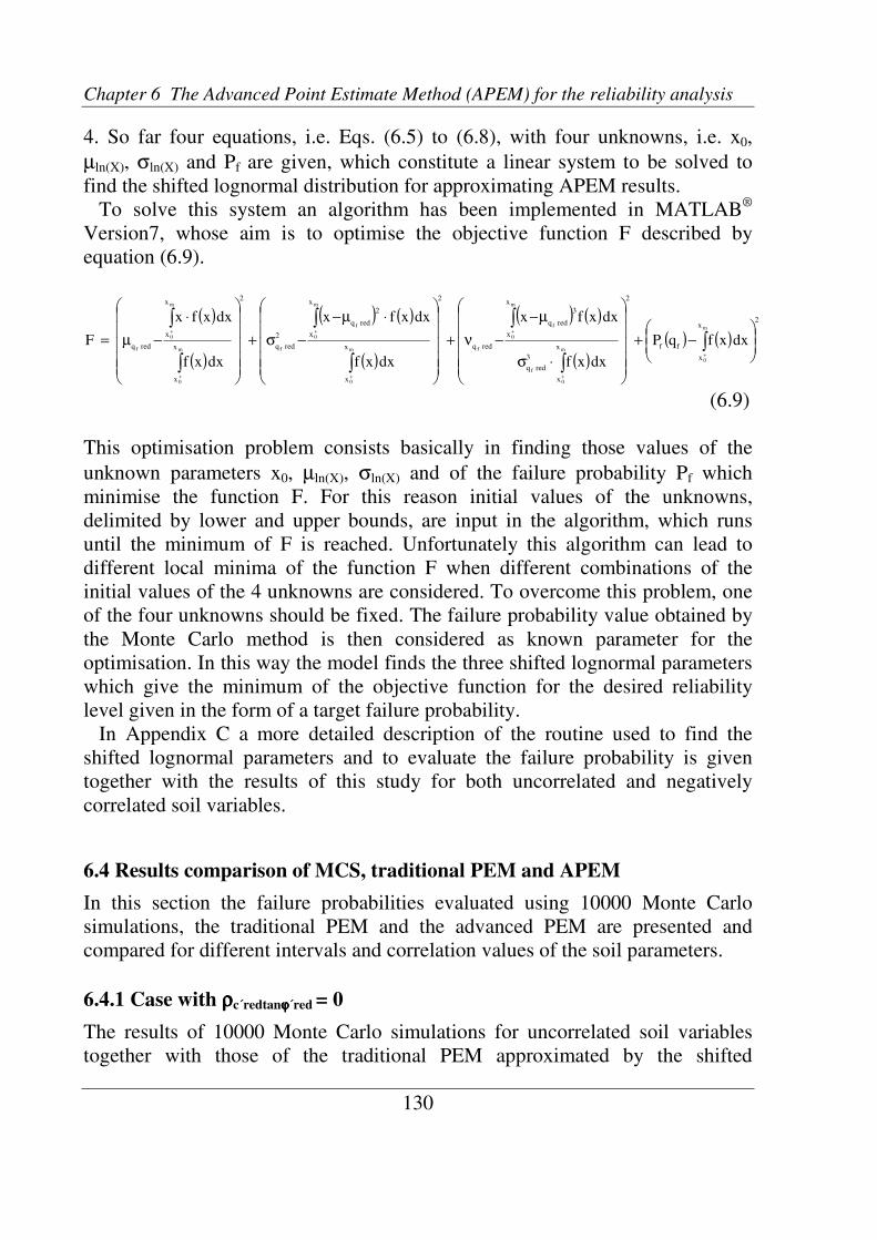
Chapter 6 The Advanced Point Estimate Method (APEM) for the reliability analysis
130
4. So far four equations, i.e. Eqs. (6.5) to (6.8), with four unknowns, i.e. x0,
µln(X), σln(X) and Pf are given, which constitute a linear system to be solved to
find the shifted lognormal distribution for approximating APEM results.
To solve this system an algorithm has been implemented in MATLAB®
Version7, whose aim is to optimise the objective function F described by
equation (6.9).
( )
( )
( ) ( )
( )
( ) ( )
( )
( ) ( )
2x
x
ff
2
x
x
3
redq
x
x
3
redq
redq
2
x
x
x
x
2
redq
2
redq
2
x
x
x
x
redq
m
0
m
0
f
m
0
f
fm
0
m
0
f
fm
0
m
0
fdxxfqP
dxxf
dxxfx
dxxf
dxxfx
dxxf
dxxfx
F
−+
⋅σ
µ−
−ν+
⋅µ−
−σ+
⋅
−µ= ∫∫
∫
∫
∫
∫
∫
+
+
+
+
+
+
+
(6.9)
This optimisation problem consists basically in finding those values of the
unknown parameters x0, µln(X), σln(X) and of the failure probability Pf which
minimise the function F. For this reason initial values of the unknowns,
delimited by lower and upper bounds, are input in the algorithm, which runs
until the minimum of F is reached. Unfortunately this algorithm can lead to
different local minima of the function F when different combinations of the
initial values of the 4 unknowns are considered. To overcome this problem, one
of the four unknowns should be fixed. The failure probability value obtained by
the Monte Carlo method is then considered as known parameter for the
optimisation. In this way the model finds the three shifted lognormal parameters
which give the minimum of the objective function for the desired reliability
level given in the form of a target failure probability.
In Appendix C a more detailed description of the routine used to find the
shifted lognormal parameters and to evaluate the failure probability is given
together with the results of this study for both uncorrelated and negatively
correlated soil variables.
6.4 Results comparison of MCS, traditional PEM and APEM
In this section the failure probabilities evaluated using 10000 Monte Carlo
simulations, the traditional PEM and the advanced PEM are presented and
compared for different intervals and correlation values of the soil parameters.
6.4.1 Case with ρρρρc´redtanϕϕϕϕ´red = 0
The results of 10000 Monte Carlo simulations for uncorrelated soil variables
together with those of the traditional PEM approximated by the shifted

6.4 Results comparison of MCS, traditional PEM and APEM
131
qf - interval of APEM application
APEM(150): 0 - 150 kN/m2
APEM(200): 0 - 200 kN/m2
APEM(250): 0 - 250 kN/m2
friction angle
0 - 22.5°
0 - 24.5°
0 - 24.75°
0
0.0005
0.001
0.0015
0.002
0.0025
0.003
0.0035
0.004
0.0045
0.005
0 50 100 150 200 250 300 350 400 450 500 550 600 650 700
Bearing capacity qf (kN/m^2)
Pro
bab
ilit
y d
ensi
ty f
un
ctio
n
MCS PEM APEM(250) APEM(200) APEM(150)
Bearing capacity qf (kN/m²)
0
0.0005
0.001
0.0015
0.002
0.0025
0.003
0.0035
0.004
0.0045
0.005
0 50 100 150 200 250 300 350 400 450 500 550 600 650 700
Bearing capacity qf (kN/m^2)
Pro
bab
ilit
y d
ensi
ty f
un
ctio
n
MCS PEM APEM(250) APEM(200) APEM(150)
Bearing capacity qf (kN/m²)
lognormal distribution are shown in Fig. 6.10. These results are listed,
respectively, in Table 4.5 for MCS and 5.4 for PEM. Furthermore the APEM
results, reported in Table 6.17, are also drawn assuming a shifted lognormal
distribution.
Table 6.20: Bearing capacity range of APEM application for different friction
angle intervals
Figure 6.10: Results comparison of MCS and PEM with those of APEM
considering different intervals of the friction angle and
ρc´redtanϕ´red = 0
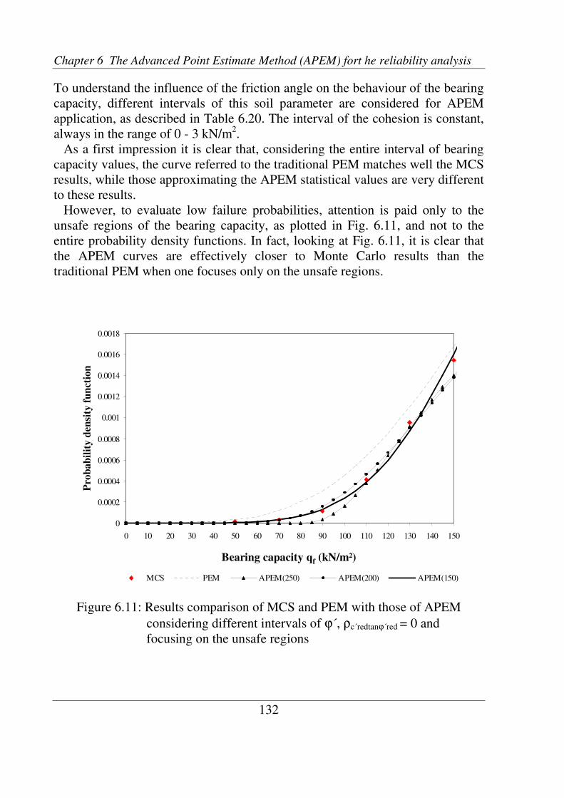
Chapter 6 The Advanced Point Estimate Method (APEM) fort he reliability analysis
132
0
0.0002
0.0004
0.0006
0.0008
0.001
0.0012
0.0014
0.0016
0.0018
0 10 20 30 40 50 60 70 80 90 100 110 120 130 140 150
Bearing capacity qf (kN/m^2)
Pro
bab
ilit
y d
ensi
ty f
un
ctio
n
MCS PEM APEM(250) APEM(200) APEM(150)
Bearing capacity qf (kN/m²)
0
0.0002
0.0004
0.0006
0.0008
0.001
0.0012
0.0014
0.0016
0.0018
0 10 20 30 40 50 60 70 80 90 100 110 120 130 140 150
Bearing capacity qf (kN/m^2)
Pro
bab
ilit
y d
ensi
ty f
un
ctio
n
MCS PEM APEM(250) APEM(200) APEM(150)
Bearing capacity qf (kN/m²)
To understand the influence of the friction angle on the behaviour of the bearing
capacity, different intervals of this soil parameter are considered for APEM
application, as described in Table 6.20. The interval of the cohesion is constant,
always in the range of 0 - 3 kN/m2.
As a first impression it is clear that, considering the entire interval of bearing
capacity values, the curve referred to the traditional PEM matches well the MCS
results, while those approximating the APEM statistical values are very different
to these results.
However, to evaluate low failure probabilities, attention is paid only to the
unsafe regions of the bearing capacity, as plotted in Fig. 6.11, and not to the
entire probability density functions. In fact, looking at Fig. 6.11, it is clear that
the APEM curves are effectively closer to Monte Carlo results than the
traditional PEM when one focuses only on the unsafe regions.
Figure 6.11: Results comparison of MCS and PEM with those of APEM
considering different intervals of ϕ´, ρc´redtanϕ´red = 0 and
focusing on the unsafe regions

6.4 Results comparison of MCS, traditional PEM and APEM
133
250 kN/m2
0.3656 0.3532 0.2565 - -
200 kN/m2
0.1767 0.1798 0.134 0.1392 -
150 kN/m2
0.0432 0.0598 0.0463 0.0437 0.0433
MCS PEM APEM(250) APEM(200) APEM(150)right extreme of qf
)0( tan =ρϕ′′ redredcfP
250 kN/m2
0.3656 0.3532 0.2565 - -
200 kN/m2
0.1767 0.1798 0.134 0.1392 -
150 kN/m2
0.0432 0.0598 0.0463 0.0437 0.0433
MCS PEM APEM(250) APEM(200) APEM(150)right extreme of qf
)0( tan =ρϕ′′ redredcfP
Table 6.21: Failure probabilities of MCS, PEM and APEM for different bearing
capacity right extreme of the unsafe region and considering
ρc´redtanϕ´red = 0
In particular, the prediction of the failure behaviour of the bearing capacity is
remarkably improved by the optimisation on the shifted lognormal parameters,
especially for the case defined as APEM(150), i.e. when smaller values of the
friction angle are considered. This demonstrates how the assumed range of the
friction angle can influence the final results of a bearing capacity reliability
analysis.
Instead, when the shifted lognormal parameter µln(X) is considered fixed, then
the model finds the failure probability values listed in Table 6.21 for different
intervals of the friction angle. These values are here compared to the failure
probabilities evaluated by means of the Monte Carlo and the traditional Point
Estimate methods.
When a failure probability is evaluated for an unsafe region, whose right
extreme is the value qf = 250 kN/m2, the traditional PEM seems to give a value
closer to that of MCS. On the other hand, when smaller unsafe region are
considered, then the APEM failure probabilities are more similar to those of
MCS. They are practically the same for reduced interval of the friction angle and
when considering the right extreme qf = 150 kN/m2.
6.4.2 Case with ρρρρc´redtanϕϕϕϕ´red = -0.6
For the case with negatively correlated soil parameters the results of 10000 MCS
are plotted pointwise in Fig. 6.12 together with those of the traditional PEM and
the APEM (applied for different friction angle intervals), approximated both by
the shifted lognormal distribution. These results are given, respectively, in Table
4.8 for MCS, Table 5.7 for PEM and Table 6.21 for APEM.
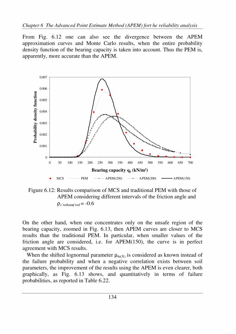
Chapter 6 The Advanced Point Estimate Method (APEM) fort he reliability analysis
134
0
0.001
0.002
0.003
0.004
0.005
0.006
0.007
0 50 100 150 200 250 300 350 400 450 500 550 600 650 700
Bearing capacity qf (kN/m^2)
Pro
ba
bil
ity
den
sity
fu
ncti
on
MCS PEM APEM(250) APEM(200) APEM(150)
Bearing capacity qf (kN/m²)
0
0.001
0.002
0.003
0.004
0.005
0.006
0.007
0 50 100 150 200 250 300 350 400 450 500 550 600 650 700
Bearing capacity qf (kN/m^2)
Pro
ba
bil
ity
den
sity
fu
ncti
on
MCS PEM APEM(250) APEM(200) APEM(150)
Bearing capacity qf (kN/m²)
From Fig. 6.12 one can also see the divergence between the APEM
approximation curves and Monte Carlo results, when the entire probability
density function of the bearing capacity is taken into account. Thus the PEM is,
apparently, more accurate than the APEM.
Figure 6.12: Results comparison of MCS and traditional PEM with those of
APEM considering different intervals of the friction angle and
ρc´redtanϕ´red = -0.6
On the other hand, when one concentrates only on the unsafe region of the
bearing capacity, zoomed in Fig. 6.13, then APEM curves are closer to MCS
results than the traditional PEM. In particular, when smaller values of the
friction angle are considered, i.e. for APEM(150), the curve is in perfect
agreement with MCS results.
When the shifted lognormal parameter µln(X) is considered as known instead of
the failure probability and when a negative correlation exists between soil
parameters, the improvement of the results using the APEM is even clearer, both
graphically, as Fig. 6.13 shows, and quantitatively in terms of failure
probabilities, as reported in Table 6.22.

6.4 Results comparison of MCS, traditional PEM and APEM
135
0
0.0001
0.0002
0.0003
0.0004
0.0005
0.0006
0 10 20 30 40 50 60 70 80 90 100 110 120 130 140 150
Bearing capacity qf (kN/m^2)
Pro
ba
bil
ity
den
sity
fu
ncti
on
MCS PEM APEM(250) APEM(200) APEM(150)
Bearing capacity qf (kN/m²)
0
0.0001
0.0002
0.0003
0.0004
0.0005
0.0006
0 10 20 30 40 50 60 70 80 90 100 110 120 130 140 150
Bearing capacity qf (kN/m^2)
Pro
ba
bil
ity
den
sity
fu
ncti
on
MCS PEM APEM(250) APEM(200) APEM(150)
Bearing capacity qf (kN/m²)
Figure 6.13: Results comparison of MCS and PEM with those of APEM
considering different intervals of ϕ´, with ρc´redtanϕ´red = -0.6
and focusing on the unsafe regions
On the other hand, when one concentrates only on the unsafe region of the
bearing capacity, zoomed in Fig. 6.13, then APEM curves are closer to MCS
results than the traditional PEM. In particular, when smaller values of the
friction angle are considered, i.e. for APEM(150), the curve is in perfect
agreement with MCS results.
When the shifted lognormal parameter µln(X) is considered as known instead of
the failure probability and when a negative correlation exists between soil
parameters, the improvement of the results using the APEM is even clearer, both
graphically, as Fig. 6.13 shows, and quantitatively in terms of failure
probabilities, as reported in Table 6.22.
The observations of the failure probability values calculated for uncorrelated
soil variables are valid also when ρc´redtanϕ´red = -0.6, except that now the failure
probability given by APEM(150) considering the right extreme qf = 150 kN/m2
is exactly the same as the value estimated using 10000 MCS.

Chapter 6 The Advanced Point Estimate Method (APEM) for the reliability analysis
136
)6.0( tan −=ρϕ′′ redredcfP
250 kN/m2
0.2686 0.2885 0.1330 - -
200 kN/m2
0.0601 0.0866 0.0345 0.0551 -
150 kN/m2
0.0015 0.0117 0.0029 0.0016 0.0015
APEM(150)right extreme of qf MCS PEM APEM(250) APEM(200)
)6.0( tan −=ρϕ′′ redredcfP
250 kN/m2
0.2686 0.2885 0.1330 - -
200 kN/m2
0.0601 0.0866 0.0345 0.0551 -
150 kN/m2
0.0015 0.0117 0.0029 0.0016 0.0015
APEM(150)right extreme of qf MCS PEM APEM(250) APEM(200)
Table 6.22: Failure probabilities of MCS, PEM and APEM for different bearing
capacity right extreme of the unsafe region and considering
ρc´redtanϕ´red = -0
Summarising all the findings about the APEM, it can then be concluded that this
new promising probabilistic approach gives excellent predictions of the failure
behaviour of the bearing capacity, especially when negatively correlated soil
parameters and reduced friction angle intervals are considered.
6.5 Applicability of the estimated failure probability of the bearing capacity
After having estimated the failure probability of the bearing capacity problem in
the previous chapter, the next step is to assess whether it is an acceptable value
or not.
Typically, this is achieved through comparing the computed failure
probabilities with a probabilistic design criterion or using diagrams usually used
in decision-making, such as the one of BAECHER (1982) shown in Fig. 6.14.
This kind of diagrams has proven to be a useful tool for describing the meaning
of failure probabilities and risks in the context of other risks familiar to the
society.
In Fig. 6.14 the annual failure probability of well-known engineering
structures is plotted against the cost in dollars or the number of lives lost in a
year. Both axes are in logarithmic scale.
This experimental diagram reveals the rates of failure and costs that the
society finds acceptable, or, can live with nowadays.
In particular for foundations, the annual failure probability considered as
acceptable by the society is included in the range 10-2
– 10-3
, thus having, for
example, a higher frequency of failure than dams, but lower annual lost of lives
and money.

6.5 Applicability of the estimated failure probability of the bearing capacity
137
For the strip footing of the bearing capacity problem it has been seen in Tables
6.21 and 6.22 that a magnitude order of 10-1
– 10-3
is found when the unsafe
region has a right extreme of the bearing capacity equals to 250 kN/m2. Whereas
this order of magnitude decreases down to 10-2
– 10-3
when the right extreme is
150 kN/m2. Hence the failure probabilities evaluated for the bearing capacity
problem seem to be realistic when compared with the annual failure rates
indicated in the diagram of Fig.6.14.
In any case, whenever one is dealing with estimated failure probabilities, it
must be clear that these values have to be considered as lower bounds of the real
failure probabilities. This is due to the fact that some effects of important
factors, which might cause failure, are perhaps ignored in the reliability analysis.
Thus engineers should be careful not to be too confident in the computed failure
probabilities.
Figure 6.14: Annual failure probability versus annual risk cost in dollars and
number of lives lost for various engineering structures
(BAECHER, 1982)

139
Chapter 7
Conclusions and further research
Introduction The aim of this research was to give a further contribution to the application of
well-known probabilistic methods to the study of the bearing capacity problem,
showing that a probabilistic analysis does not require more effort than that
needed in a conventional deterministic study, but it provides a very useful means
of modelling uncertainties involved in the calculations.
It is fundamental for engineers to ensure safety and reliability of geotechnical
structures. Another important aim of this work was to find a method able to
evaluate small failure probabilities of the bearing capacity. As a consequence,
the Advanced Point Estimate Method, described in chapter 6, was developed.
This was a big challenge. For this reason the author hopes that this promising
tool can be applied to a more comprehensive reliability analysis, helping
engineers in interpreting the probabilistic results and, thus, representing a new
perspective in the field of geotechnical engineering.
In the next sections the most important conclusions of the present thesis will
be given, followed by some recommendations for further research.
7.1 General conclusions
In chapter 2 the primary sources and types of uncertainties, which strongly
affect geotechnical engineering, were described. In spite of the advances in
modern computational resources and information technology for dealing with
uncertainties, the knowledge of engineers on uncertain parameters involved in a
design remains imperfect. As CHRISTIAN (2004) pointed out, uncertainty can
be ignored by applying the deterministic approach, with the risk of being too
conservative, thus leading to too expensive projects. On the other hand
engineers can decide to quantify uncertainties, thus contributing to a more
rational reliability analysis. It was seen that probabilistic and statistical analyses
are a powerful means for dealing with uncertainties, providing them with a more
logical mathematical framework. In spite of the reluctance of experts in applying
probabilistic concepts and methods, in recent years these techniques are finding
increasing application in the geotechnical field.
Chapter 7 Conclusions and recommendations for further research
140
In chapters 3 the methodology of the most widely known probabilistic methods
were exhaustively illustrated and their advantages and limitations were
discussed.
7.2 Conclusions with respect to the probabilistic methods applied to the
bearing capacity problem
In chapter 4 well-known probabilistic methods were applied to the study of two
benchmarks on the bearing capacity of a strip footing on a homogeneous soil
layer, considering different correlation coefficients between the soil parameters.
It has been shown that the Monte Carlo approach requires only fundamental
knowledge of statistics and probability theory to solve the bearing capacity
problem. It is generally considered as the most accurate and reliable
probabilistic method, because not only mean value, standard deviation and
skewness coefficient of a certain performance function can be obtained, but also
the corresponding probability distribution can be built up. However, as for
practical problems this method is too time consuming, other approaches were
considered.
The moments methods FOSM and SOSM were chosen as alternative
approaches to replace the Monte Carlo simulations, because they involved a
limited amount of calculations. In spite of the similar results in terms of mean
value and standard deviation with MCS, these methods did not provide any
skewness coefficient of the bearing capacity, as Monte Carlo did. Thus, no
information was given about the shape of the probability density function of the
bearing capacity. It had to be assumed to approximate the final results. In
addition, these approaches are generally accurate only for linear functions, thus
the accuracy diminishes as the non-linearity of a function increases. Since the
bearing capacity is a highly non-linear function of the effective friction angle,
then some inaccuracies were introduced in the final results of FOSM and SOSM
methods. Consequently, it was necessary to choose another probabilistic
alternative, which could be able to overcome the drawbacks of MCS, FOSM and
SOSM methods, providing the skewness coefficient together with the other
statistical estimates, but with less computational effort than Monte Carlo
method.
7.3 Conclusions with respect to the Two Point Estimate Method
141
7.3 Conclusions with respect to the Two Point Estimate Method
In chapter 5 the Two Point Estimate Method after ROSENBLUETH (1975) was
applied to the bearing capacity problem and the results were compared with
those of MCS, FOSM and SOSM methods.
Similar results were obtained for all the probabilistic methods applied in terms
of mean value and standard deviation of the bearing capacity. On the other hand,
different conclusions can be drawn for the skewness coefficient. Actually, the
First Order Second Moment and the Second Order Second Moment methods did
not allow the evaluation of the skewness coefficient, thus being substantially
less accurate than the Point Estimate Method. Moreover, a significant difference
was observed between the skewness coefficients provided by the PEM and the
Monte Carlo method.
However, it is important to stress that the PEM significantly decreased the
computational effort of the probabilistic study of the bearing capacity problem.
In fact, on one hand, the PEM did not involve the evaluation of partial
derivatives of the bearing capacity formula, thus being more straightforward
applied than FOSM and SOSM methods. On the other hand, when both soil
cohesion and friction angle were considered as input variables (i.e. in
benchmark 2), at least ten thousands of Monte Carlo simulations were necessary
to get accurate statistical values of the bearing capacity, while only four
calculations were required by the PEM to get results as accurate and reliable as
those of the Monte Carlo method in terms of mean value and standard deviation.
In the last decades, the PEM is finding increasing application in practical
problems and efforts are carried out to implement this method in finite elements
codes. However experts, who are familiar with the mathematical background of
this method, suggest the use of the PEM only under special conditions, for
which it is expected to give good results. These conditions were mentioned in
chapter 5 and are summarised here:
a) in order to reduce the error in the PEM results, the variation coefficient of the
input random variables should not be large. For the probabilistic analysis of the
bearing capacity problem a variation coefficient of 80% was taken into account
for the soil cohesion, which is larger than the values usually found in the
literature;
b) when multiple input random variables are considered, the skewness
coefficient can only be reliably calculated by applying formula (3.17) of the
PEM after ROSENBLUETH if the variables are uncorrelated and if the
performance function is linear, which is not the case for the bearing capacity
formula;
Chapter 7 Conclusions and recommendations for further research
142
c) to cope with the problem of condition b), different formulas are available in
the literature to evaluate the sampling point weights of the PEM for correlated
input parameters, such as those proposed by CHRISTIAN et al. (1999) and
shown in chapter 3. Unfortunately these formulas are valid only for symmetrical
input variables. Thus, one should be careful in applying them to cases in which
the transformation of an input variable changes its distributional form. In this
research, in fact, in order to apply CHRISTIAN’s formula, the lognormal soil
cohesion c´ had to be transformed into the normal variable lnc´. So doing, the
correlation coefficient between the input soil variables cohesion and friction
angle changed, because of the different mean value and standard deviation of c´
and lnc´, thus influencing the evaluation of the sampling point weights.
These three conditions influenced the probabilistic results of the bearing
capacity problem, thus being the primary reason of the difference between the
skewness estimates of the PEM and the MCS. Despite its limitations, the PEM
was shown to be a simple, but powerful technique for probabilistic analysis, as it
required less computational effort than MCS for a comparable degree of
accuracy.
7.4 Conclusions with respect to the shifted lognormal distribution
In chapter 5 the importance of assuming a certain probability density function as
opposed to others to approximate and plot the results of the probabilistic
analysis of the bearing capacity problem were discussed.
Considering the Monte Carlo results, it was possible to define the shape of the
bearing capacity density function. In fact, from these results it was clear that a
reasonable assumption for the bearing capacity estimates should be a positively
(right) skewed probability distribution.
Different continuous probability distributions are available in the literature to
approximate these results. In Geotechnics the Gaussian normal and the standard
lognormal distributions are frequently used, because of their mathematical
simplicity. Furthermore, the necessary statistical information about these
functions is widely available, including probability tables.
In this research, the shifted lognormal distribution was chosen to plot the
probability distribution of the bearing capacity, not only because it is strictly
non-negative and can be treated mathematically straightforward, but especially
because it matches well all the three moments of the bearing capacity, i.e. mean
value, standard deviation and skewness. Hence, the final approximation is more

7.5 Conclusions with respect to the correlation between the soil parameters c´ and tanφ´
143
accurate and reliable than other probability density functions. This represents
one of the most basic findings of this work.
Other good reasons for preferring the shifted lognormal distribution to other
well-known continuous probability density curves are listed below:
- the first term of the bearing capacity formula (A.4) after Terzaghi is given as
the product of the soil parameters c´ and tanϕ´. For the central limit theorem, the
distribution of the bearing capacity should then tend to a lognormal distribution;
- generally the Gaussian distribution allows negative values of a certain
performance function, which is physically unrealistic for soil parameters. For
this reason this distribution could only be considered as a rough approximation;
- the Weibull distribution presented a high discrepancy with the other functions
considered in this work. In addition, as this distribution is usually truncated at a
lower bound, it did not describe the entire interval of the bearing capacity
results, as the others did;
- for the reliability analysis of the bearing capacity problem, the shifted
lognormal distribution showed to be the best fit-curve of all considered for
approximating MCS results, leading to failure probabilities in good agreement
with those evaluated using the Monte Carlo method.
It can be concluded that the shifted lognormal distribution was shown to be an
important and useful density curve for approximating the results of a
probabilistic analysis. As there is little information about the application of this
function in geotechnical literature, it is suggested that the shifted lognormal
distribution has to be considered for further probabilistic studies.
7.5 Conclusions with respect to the correlation between the soil parameters
c´ and tanϕϕϕϕ´
Another important finding in this research refers to the correlation between the
soil parameters cohesion and friction angle. In the literature some authors have
often based their probabilistic studies considering uncorrelated parameters to
simplify calculations, thus being more conservative. Other authors found
negative correlation between cohesion and friction angle on the basis of
experimental data. However, in geotechnical literature it is hard to find
Chapter 7 Conclusions and recommendations for further research
144
probabilistic studies based on the assumption of a negative correlation between
soil parameters.
In this work, different correlations between cohesion and friction angle was
taken into account for the probabilistic analysis of the bearing capacity.
Independent of the probabilistic method applied, a lower bearing capacity
variability was shown in chapter 5 and much lower failure probabilities
(conversely, much higher reliability indeces) were found in chapter 6 when a
negative correlation is considered, thus affecting the final results of the
probabilistic and reliability analyses significantly.
It can be then concluded that the choice of a negative correlation between soil
parameters is reasonable, because the uncertainty in the probabilistic analysis is
effectively reduced and the reliability level strongly increased.
7.6 Conclusions with respect to the reliability analysis
In chapter 6 the results of the reliability analysis of the bearing capacity problem
were shown in terms of failure probability and reliability index for both
uncorrelated and negatively correlated soil parameters. All the probabilistic
methods described in chapter 3 were applied and the corresponding results were
then compared.
Since many parameters are not incorporated in the reliability analysis to
simplify calculations, then the estimated failure probability, referred to the
lifetime of the shallow foundation, should be considered as a lower bound to the
absolute probability of failure. If a more elaborate probabilistic risk analysis
would be executed, taking into account all the uncertain contingencies, then the
absolute risk could be evaluated.
Initially the Monte Carlo method was considered to evaluate the failure
probability of the bearing capacity. It was found that, increasing the simulations
number, the failure probability decreased thus increasing the reliability level.
The MCS were easily applied to the non-linear performance function “bearing
capacity”. However, in practice, when the target failure probability is very small
and a correlation between the input variables is taken into account, the number
of simulations required to obtain an accurate result can be so large that it renders
the application impractical.
For this reason, the PEM, FOSM, SOSM and FORM methods were also
applied to evaluate the reliability of the bearing capacity. As these approaches
did not provide any probability density function, one had to assume a certain
distribution to plot the bearing capacity results and then estimate the
corresponding failure probability by integrating over the unsafe region of the

7.7 Conclusions with respect to the APEM
145
assumed density function. In this way, estimates of the failure probability are
highly sensitive to the assumed distribution.
Moreover, the approximation procedures FORM, FOSM and SOSM showed
some additional drawbacks in the reliability analysis of the bearing capacity
problem. First of all, the iterative procedure of the FORM method overestimated
the failure probability when compared with MCS results. This is due to the fact
that the bearing capacity is highly non-linear with tanϕ´, which is one of the
input variables that play an important role in this analysis. In fact, it is well-
known that a linear approximation in the FORM design point causes some
serious error in the estimation of the reliability index, thus influencing also the
value of the failure probability. One should therefore be very careful in applying
the approximation procedures of FORM, FOSM and SOSM in the reliability
analysis of a structure that has a highly non-linear performance function, such as
a shallow foundation design. In addition, the input variable cohesion follows a
distribution, which is far from the normal distribution for which the FORM
method can be applied, thus introducing additional uncertainties in the final
results when this is transformed to a normal variable.
Furthermore, as all of these methods did not provide any skewness, then their
results could not be approximated by the shifted lognormal distribution, which
proved to be the best-fit curve for MCS results, also in term of failure
probabilities.
The PEM, as a direct non-iterative method, overcomes the convergence
problem of FORM, and provides a value for the skewness coefficient, thus being
a more promising alternative. Hence, only the PEM failure probabilities were
considered to be compared with those of the MCS. Unfortunately, these values
were in this analysis even higher than those of FORM method, when compared
with the real failure probability values of MCS.
It can be concluded that, apparently, the FORM method showed to give better
failure probability results than PEM. However FORM estimates were found by
considering a normal distribution, which is not the best-fit curve for
approximating MCS results.
7.7 Conclusions with respect to the APEM
In order to overcome the drawback of the PEM for the assessment of low failure
probabilities, a so called advanced PEM, or shortly APEM, was developed. This
method is not yet available in the literature.
The basic idea of the APEM is to focus on the relatively small values of the
cohesion and the friction angle, which could cause most probably bearing
Chapter 7 Conclusions and recommendations for further research´
146
capacity failure. The reduced intervals of the soil parameters were found using
an iterative procedure. The PEM was then applied to these intervals and the
results were approximated by the shifted lognormal distribution to evaluate a
target failure probability.
It was seen that, reducing the interval of the friction angle, the failure
probability decreased. On the other hand, the width of the cohesion interval was
shown not to have a great influence on the bearing capacity results.
This new promising probabilistic approach was shown to give the best
predictions of the failure behaviour of the bearing capacity when compared with
the traditional PEM, FOSM, SOSM and SOSM methods and excellent estimates
when compared with MCS, especially if negatively correlated soil parameters
were considered.
The application of the proposed method on the bearing capacity problem was
feasible, since the mathematical and probabilistic background required to
understand its methodology is not very complicated. Furthermore, the idea of
considering reduced intervals of the cohesion and the friction angle is in practice
more logical for the evaluation of small failure probabilities of the bearing
capacity. Therefore the APEM should be easily accepted by practical engineers.
7.8 Recommendations for further research
The application of well-known probabilistic methods to the bearing capacity
problem showed the necessity of providing a mathematical framework for
dealing with uncertainties in a more rational manner. Combining the traditional
deterministic approach and the probabilistic analysis in further research can be
beneficial to geotechnical engineering practice, supporting engineering
judgement and improving the decision-making process.
Also, the proposed APEM could in future be an important tool for evaluating
small failure probabilities of geotechnical structures. Therefore, the next step
should be an user-friendly implementation of this approach into finite element
codes and its extension to some real case studies, such as the slope stability
problem. This would improve its applicability in practical design and allow a
more definitive judgement on its advantages and limitations.
It must be clear that this research showed the results of a simplified probabilistic
analysis of the bearing capacity problem, ignoring some important factors of
uncertainties, such as the heterogeneity of soil properties. So doing the failure
probability can be overestimated, leading to erroneous results. Thus the next

7.8 Recommendations for further research
147
challenge is to include the APEM into more complex geotechnical models (e.g.
highly non-linear; 3D) considering all significant sources of uncertainty, such as
the inherent spatial variability of soil parameters.

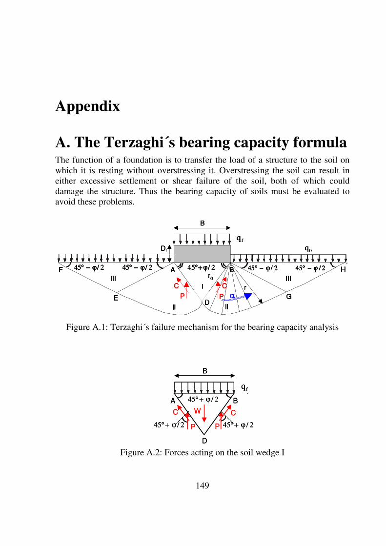
149
A 2/45 ϕ+°
CC
PP
B
D
W
B
fq
2/45 ϕ+° 2/45 ϕ+°
A 2/45 ϕ+°
CC
PP
B
D
W
B
fq
2/45 ϕ+° 2/45 ϕ+°
B
2/45 ϕ−° 2/45 ϕ−°
fq
0qDf
2/45 ϕ+°2/45 ϕ−° 2/45 ϕ−°
CC
PP
IIII
III III
A B
E
F
G
Hr0
rα
D
B
2/45 ϕ−° 2/45 ϕ−°
fq
0qDf
2/45 ϕ+°2/45 ϕ−° 2/45 ϕ−°
CC
PP
IIII
III III
A B
E
F
G
Hr0
rα
D
I
B
2/45 ϕ−° 2/45 ϕ−°
fq
0qDf
2/45 ϕ+°2/45 ϕ−° 2/45 ϕ−°
CC
PP
IIII
III III
A B
E
F
G
Hr0
rα
D
B
2/45 ϕ−° 2/45 ϕ−°
fq
0qDf
2/45 ϕ+°2/45 ϕ−° 2/45 ϕ−°
CC
PP
IIII
III III
A B
E
F
G
Hr0
rα
D
I
Appendix
A. The Terzaghi´s bearing capacity formula The function of a foundation is to transfer the load of a structure to the soil on
which it is resting without overstressing it. Overstressing the soil can result in
either excessive settlement or shear failure of the soil, both of which could
damage the structure. Thus the bearing capacity of soils must be evaluated to
avoid these problems.
Figure A.1: Terzaghi´s failure mechanism for the bearing capacity analysis
Figure A.2: Forces acting on the soil wedge I

Appendix A The Terzaghi´s bearing capacity formula
150
The failure mechanism assumed by TERZAGHI (1943) for determining the
ultimate bearing capacity of a shallow foundation is shown in Fig. A.1. The soil-
zone I is an elastic zone, zones III are the radial shear zones and zones II are arcs
of a logarithmic spiral, whose equation is given as
( ) ϕ′⋅α−α
⋅=tan
0
0err (A.1)
The lines EF and GH are straight lines. If the load per unit area qf is applied to
the shallow foundation and general shear failure occurs, the passive force P is
acting on each of the faces of the soil wedge ABD.
Considering the soil wedge I and a unit length of the foundation, as in Fig.
A.2, one has for equilibrium conditions
P2sinC2W1Bqf
⋅+ϕ′⋅⋅+−=⋅⋅ (A.2)
where
forcepassiveKtan2
BqKtan
2
BcKtan
2
B
2
1P
forcecohesivecos
2/BcC
wedgesoiltheofweighttan4
BW
q0c
2
2
=
ϕ′⋅⋅+⋅
ϕ′⋅+⋅
ϕ⋅⋅γ⋅=
=ϕ′
⋅=
=ϕ′⋅⋅γ=
γ&
(A.3)
Kq, Kc and Kγ are earth pressure coefficients depending on the soil friction angle
which are very tedious to evaluate. Introducing the values of Eqs. (A.3) in Eq.
(A.2) the ultimate bearing capacity equation will be then given by
γ⋅⋅γ⋅+⋅+⋅= NB
2
1NqNcq
q0cf (A.4)
where c is the soil cohesion, q0 is the surcharge (or overburden stress), γ is the
unit soil weight, B is the footing width and Nq, Nc and Nγ are the bearing
capacity factors defined by the following equations:

Appendix A The Terzaghi´s bearing capacity formula
151
( ) ( )
( ) ( ) )1961(HANSENBRINCHaftertan1N8.11tanK2
tanN
)1921(PRANDTLaftercot1Ntan1KN
)1921(PRANDTLafter24
tanetanKN
q
qcc
2tan
−ϕ′⋅−⋅=−ϕ′⋅⋅ϕ′
=
ϕ′⋅−=ϕ′⋅+=
ϕ′+
π⋅⋅=ϕ′⋅=
γγ
ϕ′⋅π
(A.5)
Equation (A.4) shows in a simple way that the ultimate bearing capacity is a
function of three contributions, i.e. the soil weight inside the failure surface, the
soil cohesion acting along the failure surface and the surcharge applied at the
surface.
The bearing capacity factors depend on the friction angle of the soil. The
equations (A.5) for evaluating Nq and Nc were first obtained by PRANDTL
(1921), which are exact closed-form solutions obtainable using the limit
analyses. In the German literature these two factors are denoted respectively as
Nd and Nc.
On the other hand no closed-form solution exists forγ
N and the equation (A.5)
for this factor is only one of the approximations available in the literature. The
difference between these solutions is up to a factor of two, depending on the
wedge angle below the foundation.
The first solution for γ
N was obtained by CAQUOT and KERISEL (1953) and
can be expressed in the form
( ) ϕ′⋅−⋅=γ
tan1N2Nq
(A.6)
Equation (A.6) is for example applied in the EUROCODE 7 (1994). This
formula has been further extended by BRINCH-HANSEN (1970), as given in
Eq. (A.5). This solution is considered in this work for the evaluation of the
bearing capacity.
In the German literature the bearing capacity factor γ
N obtained by
MEYERHOF (1963), denoted as Nb, is applied, which can be evaluated with the
following equation
( ) ( )ϕ′⋅⋅−==γ
4.1tan1NNNqb
(A.7)
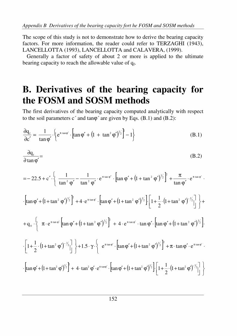
Appendix B Derivatives of the bearing capacity fort he FOSM and SOSM methods
152
The scope of this study is not to demonstrate how to derive the bearing capacity
factors. For more information, the reader could refer to TERZAGHI (1943),
LANCELLOTTA (1993), LANCELLOTTA and CALAVERA, (1999).
Generally a factor of safety of about 2 or more is applied to the ultimate
bearing capacity to reach the allowable value of qf.
B. Derivatives of the bearing capacity for
the FOSM and SOSM methods The first derivatives of the bearing capacity computed analytically with respect
to the soil parameters c´ and tanϕ´ are given by Eqs. (B.1) and (B.2):
( )[ ]
−ϕ′++ϕ′⋅⋅ϕ′
=′∂
∂ϕ′⋅π
1tan1tanetan
1
c
q 22
12tanf (B.1)
=ϕ′∂
∂
tan
qf (B.2)
( )[ ] ⋅⋅ϕ′
π+ϕ′++ϕ′⋅⋅
ϕ′−
ϕ′⋅′+−=
ϕ′⋅πϕ ′′⋅π tan2
21
2tan
22e
tantan1tane
tan
1
tan
1c5.22
( )[ ] ( )[ ] ( ) +
ϕ′+⋅+⋅ϕ′++ϕ′⋅⋅+ϕ′++ϕ′⋅
−ϕ′⋅π 21
221
2tan2
21
2 tan12
11tan1tane4tan1tan
( )[ ] ( )[ ]⋅ϕ′++ϕ′⋅ϕ′⋅⋅+ϕ′++ϕ′
⋅π⋅+ϕ′⋅π⋅ϕ′⋅π 2
12tan
22
12tan
0tan1tantane4tan1taneq
( ) ( )[ ] ⋅⋅ϕ′⋅π+ϕ′++ϕ′⋅
⋅γ⋅+
ϕ′+⋅+⋅
ϕ′⋅πϕ′⋅π− tan2
21
2tan21
2 etantan1tane5.1tan12
11
( )[ ] ( )[ ] ( )
ϕ′+⋅+⋅ϕ′++ϕ′⋅⋅ϕ′⋅+ϕ′++ϕ′⋅
−ϕ′⋅π 21
221
2tan22
21
2tan1
2
11tan1tanetan4tan1tan

Appendix B Derivatives of the bearing capacity for the FOSM and SOSM methods
153
The second derivatives of the bearing capacity computed analytically with
respect to the soil parameters c´ and tanϕ´ are given by Eqs. (B.3) and (B.4):
0c
q2
f
2
=′∂
∂ (B.3)
=ϕ′∂
∂
tan
q2
f
2
(B.4)
( )[ ] ( )[ ] ( )[ ]−ϕ′++ϕ′⋅ϕ′
π−ϕ′++ϕ′⋅
ϕ′⋅ϕ′++ϕ′⋅⋅′+
ϕ′
′⋅−=
ϕ′⋅π 21
2
2
21
2
3
21
2tan
3tan1tan
tantan1tan
tan
2tan1tanec
tan
c2
( ) ( )[ ] ( )[ ]+ϕ′++ϕ′⋅ϕ′
π+
ϕ′++ϕ′⋅
ϕ′−⋅π+
ϕ′+⋅+⋅
ϕ′−
−2
122
12
2
21
2tan1tan
tantan1tan
tan
1tan1
2
11
tan
4
( ) ( ) ( ) ( ) +
ϕ′+⋅−⋅ϕ′+
ϕ′+⋅+⋅ϕ′⋅+
ϕ′+⋅+⋅π⋅+
ϕ′+⋅+⋅+
−−−−2
32
2
21
221
221
2 tan12
1tantan1
2
11tan2tan1
2
114tan1
2
114
( )[ ] ( )[ ] ( ) +
ϕ′+⋅+⋅ϕ′++ϕ′⋅ϕ′⋅+ϕ′++ϕ′⋅π⋅⋅π⋅+
−ϕ′⋅π 21
221
22
21
2tan tan12
11tan1tantan4tan1taneq
( )[ ] ( ) ( )[ ]+ϕ′++ϕ′⋅⋅+
ϕ′+⋅+⋅ϕ′++ϕ′⋅ϕ′⋅
⋅π⋅+
ϕ′⋅π−ϕ′⋅π 21
2tan21
221
2tantan1tan2etan1
2
11tan1tantane4
( )[ ] ( ) ( ) ( )[ ]
ϕ′++ϕ′⋅
ϕ′+⋅−⋅⋅ϕ′+
ϕ′+⋅+⋅ϕ′+⋅ϕ′+
−ϕ′⋅π−−2
122
32tan22
122
122 tan1tantan1
2
1etantan1
2
11tan1tan
( )[ ] ( )[ ] ( ) +
ϕ′+⋅+⋅ϕ′++ϕ′⋅ϕ′⋅+ϕ′++ϕ′⋅π
⋅⋅+−ϕ′⋅π 2
122
12
22
12tan tan1
2
11tan1tantan4tan1tane5.22
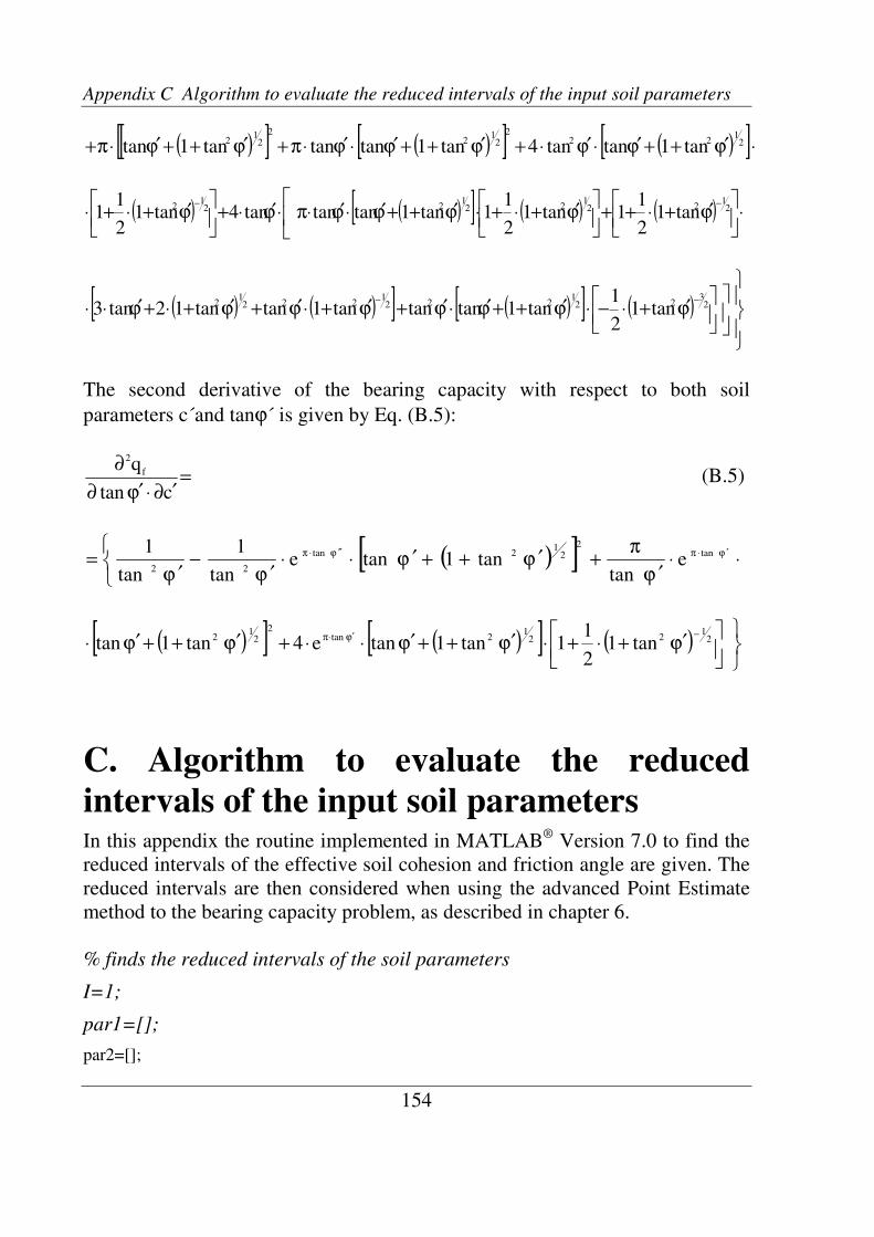
Appendix C Algorithm to evaluate the reduced intervals of the input soil parameters
154
( )[ ][ ( )[ ] ( )[ ]⋅ϕ′++ϕ′⋅ϕ′⋅+ϕ′++ϕ′⋅ϕ′⋅π+ϕ′++ϕ′⋅π+ 21
222
21
22
21
2 tan1tantan4tan1tantantan1tan
( ) ( )[ ] ( ) ( ) ⋅
ϕ′+⋅++
ϕ′+⋅+
⋅ϕ′++ϕ′⋅ϕ′⋅π⋅ϕ′⋅+
ϕ′+⋅+⋅
−−2
122
122
122
12
tan12
11tan1
2
11tan1tantantan4tan1
2
11
( ) ( )[ ] ( )[ ] ( )
ϕ′+⋅−⋅ϕ′++ϕ′⋅ϕ′+ϕ′+⋅ϕ′+ϕ′+⋅+ϕ′⋅⋅
−−2
322
1222
1222
12 tan1
2
1tan1tantantan1tantan12tan3
The second derivative of the bearing capacity with respect to both soil
parameters c´and tanϕ´ is given by Eq. (B.5):
=′∂⋅ϕ′∂
∂
ctan
qf
2
(B.5)
( )[ ] ⋅⋅ϕ ′
π+ϕ ′++ϕ ′⋅⋅
ϕ ′−
ϕ ′=
ϕ ′⋅πϕ ′′⋅π tan2
21
2tan
22e
tantan1tane
tan
1
tan
1
( )[ ] ( )[ ] ( )
ϕ′+⋅+⋅ϕ′++ϕ′⋅⋅+ϕ′++ϕ′⋅
−ϕ′⋅π 21
221
2tan2
21
2 tan12
11tan1tane4tan1tan
C. Algorithm to evaluate the reduced
intervals of the input soil parameters In this appendix the routine implemented in MATLAB
® Version 7.0 to find the
reduced intervals of the effective soil cohesion and friction angle are given. The
reduced intervals are then considered when using the advanced Point Estimate
method to the bearing capacity problem, as described in chapter 6.
% finds the reduced intervals of the soil parameters
I=1;
par1=[];
par2=[];
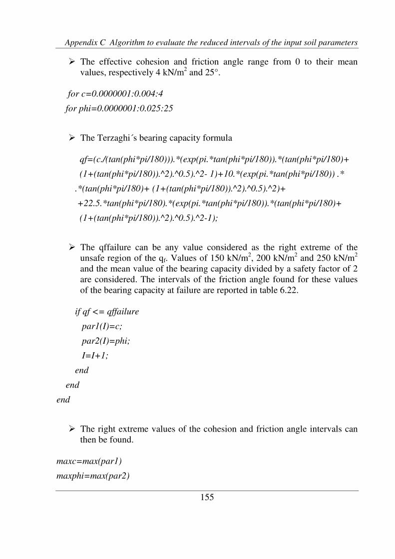
Appendix C Algorithm to evaluate the reduced intervals of the input soil parameters
155
The effective cohesion and friction angle range from 0 to their mean
values, respectively 4 kN/m2 and 25°.
for c=0.0000001:0.004:4
for phi=0.0000001:0.025:25
The Terzaghi´s bearing capacity formula
qf=(c./(tan(phi*pi/180))).*(exp(pi.*tan(phi*pi/180)).*(tan(phi*pi/180)+
(1+(tan(phi*pi/180)).^2).^0.5).^2- 1)+10.*(exp(pi.*tan(phi*pi/180)) .*
.*(tan(phi*pi/180)+ (1+(tan(phi*pi/180)).^2).^0.5).^2)+
+22.5.*tan(phi*pi/180).*(exp(pi.*tan(phi*pi/180)).*(tan(phi*pi/180)+
(1+(tan(phi*pi/180)).^2).^0.5).^2-1);
The qffailure can be any value considered as the right extreme of the
unsafe region of the qf. Values of 150 kN/m2, 200 kN/m
2 and 250 kN/m
2
and the mean value of the bearing capacity divided by a safety factor of 2
are considered. The intervals of the friction angle found for these values
of the bearing capacity at failure are reported in table 6.22.
if qf <= qffailure
par1(I)=c;
par2(I)=phi;
I=I+1;
end
end
end
The right extreme values of the cohesion and friction angle intervals can
then be found.
maxc=max(par1)
maxphi=max(par2)

Appendix D Algorithm to evaluate the shifted lognormal parameters and the failure probability
156
D. Algorithm to evaluate the shifted
lognormal parameters and the failure
probability of the bearing capacity problem The aim of this appendix is to describe the algorithm implemented in
MATLAB® Version 7.0 to evaluate the three parameters of the shifted
lognormal distribution and the failure probability of the bearing capacity
problem by considering the results of the advanced PEM shown in tables 6.19
and 6.21 of chapter 6.
The objective function F to be optimised is given by Eq. (6.8).
D.1 Main routine for the estimation of the three shifted lognormal
parameters
In the main routine the parameters of the shifted lognormal distribution,
described by Eq. (2.15), are indicated respectively as m=µln(X), s=σln(X) and u=x0,
while the failure probability is simply given by Pf=Pf.
% main program for the estimation of the shifted lognormal distribution
parameters and the failure probability of the bearing capacity problem
Initial values of the 4 unknown parameters are input together with their
corresponding lower (lb) and upper (ub) bounds to start the optimization
problem
% initial values are m, s, u, Pf
par0 = [m0 s0 u0 Pf0];
The optimset command creates an optimization option structure. More
precisely, after for example 10000 runs, it displays the output of each
iteration, checks whether the objective function F values are valid giving a
warning when the function returns an invalid value (complex or not a
number) and it displays the maximum number of function evaluations
allowed.
% options

Appendix D Algorithm to evaluate the shifted lognormal parameters and the failure probability
157
option = optimset('Display','iter','MaxFunEvals',10000);
% lower and upper bounds of the input parameters m, s, u, Pf
lb = [ml sl ul Pfl];
ub = [mu su uu Pfu];
The gradient based solver fmincon finds the constrained minimum of the
function F starting at initial bounded values par0. It returns a structure
output with information about the optimization, i.e.: par indicates the
results of the four unknowns, fval is the minimum of the function reached,
exitflag describes the exit condition of fmincon.
% minimiser of the function F
[par,fval,exitflag,output] =fmincon(@integralmod,par0,[],[],[],[],lb,ub,[],opti);
The results of the optimization problem can be displayed
% results of the shifted lognormal parameters m, s, u and of the failure
probability Pf
m = par(1)
s = par(2)
u = par(3)
Pf = par(4)
% extreme values of the integration intervals of the objective function F
x0=par(3)+0.1
xm=0.5*(par(3)+exp(par(1)+0.5*((par(2))^2)))
% statistical values of the entire shifted lognormal distribution of the bearing
capacity to be found
mean_value=par(3)+exp(par(1)+0.5*((par(2))^2))
standard_deviation=((-1+(exp(par(2)^2))^0.5))*(exp(par(1)+0.5*((par(2))^2)))
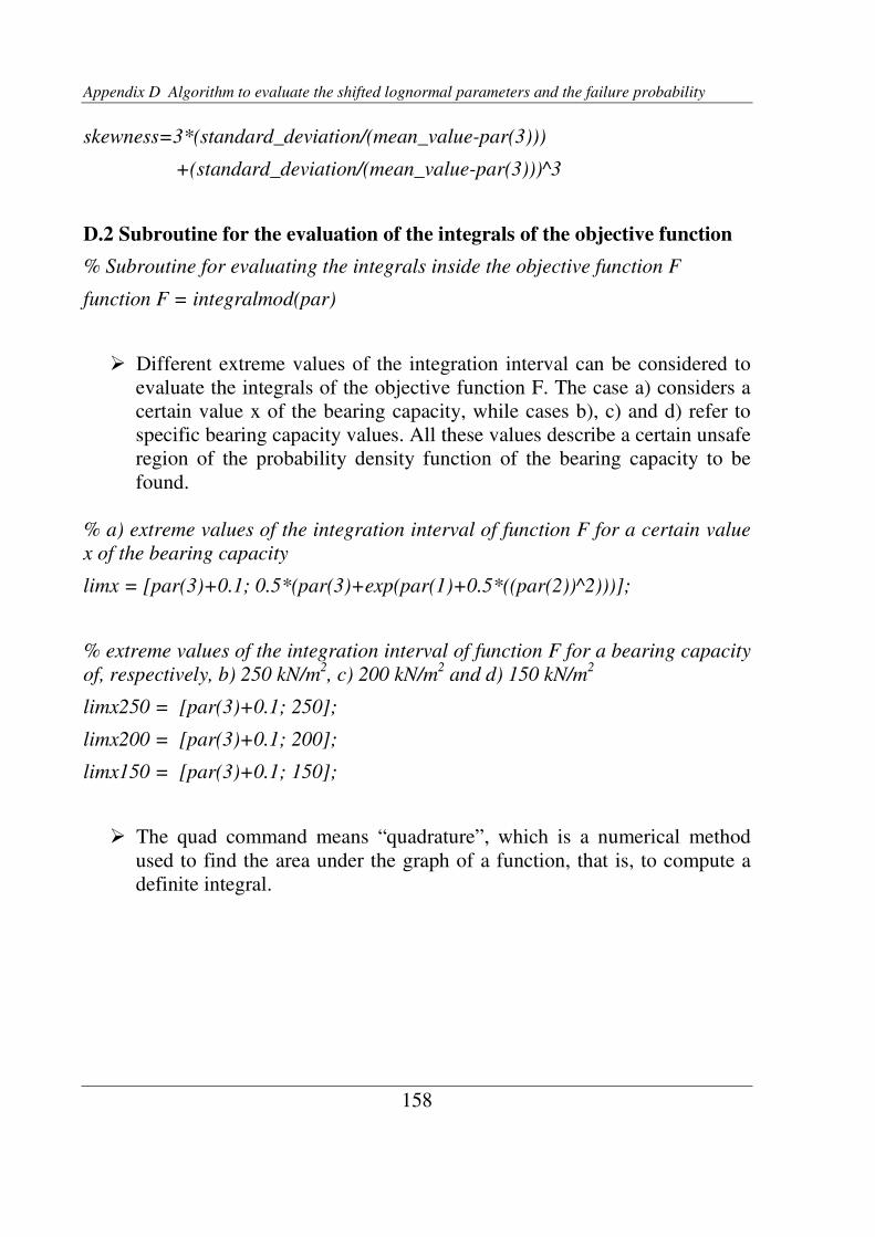
Appendix D Algorithm to evaluate the shifted lognormal parameters and the failure probability
158
skewness=3*(standard_deviation/(mean_value-par(3)))
+(standard_deviation/(mean_value-par(3)))^3
D.2 Subroutine for the evaluation of the integrals of the objective function
% Subroutine for evaluating the integrals inside the objective function F
function F = integralmod(par)
Different extreme values of the integration interval can be considered to
evaluate the integrals of the objective function F. The case a) considers a
certain value x of the bearing capacity, while cases b), c) and d) refer to
specific bearing capacity values. All these values describe a certain unsafe
region of the probability density function of the bearing capacity to be
found.
% a) extreme values of the integration interval of function F for a certain value
x of the bearing capacity
limx = [par(3)+0.1; 0.5*(par(3)+exp(par(1)+0.5*((par(2))^2)))];
% extreme values of the integration interval of function F for a bearing capacity
of, respectively, b) 250 kN/m2, c) 200 kN/m
2 and d) 150 kN/m
2
limx250 = [par(3)+0.1; 250];
limx200 = [par(3)+0.1; 200];
limx150 = [par(3)+0.1; 150];
The quad command means “quadrature”, which is a numerical method
used to find the area under the graph of a function, that is, to compute a
definite integral.
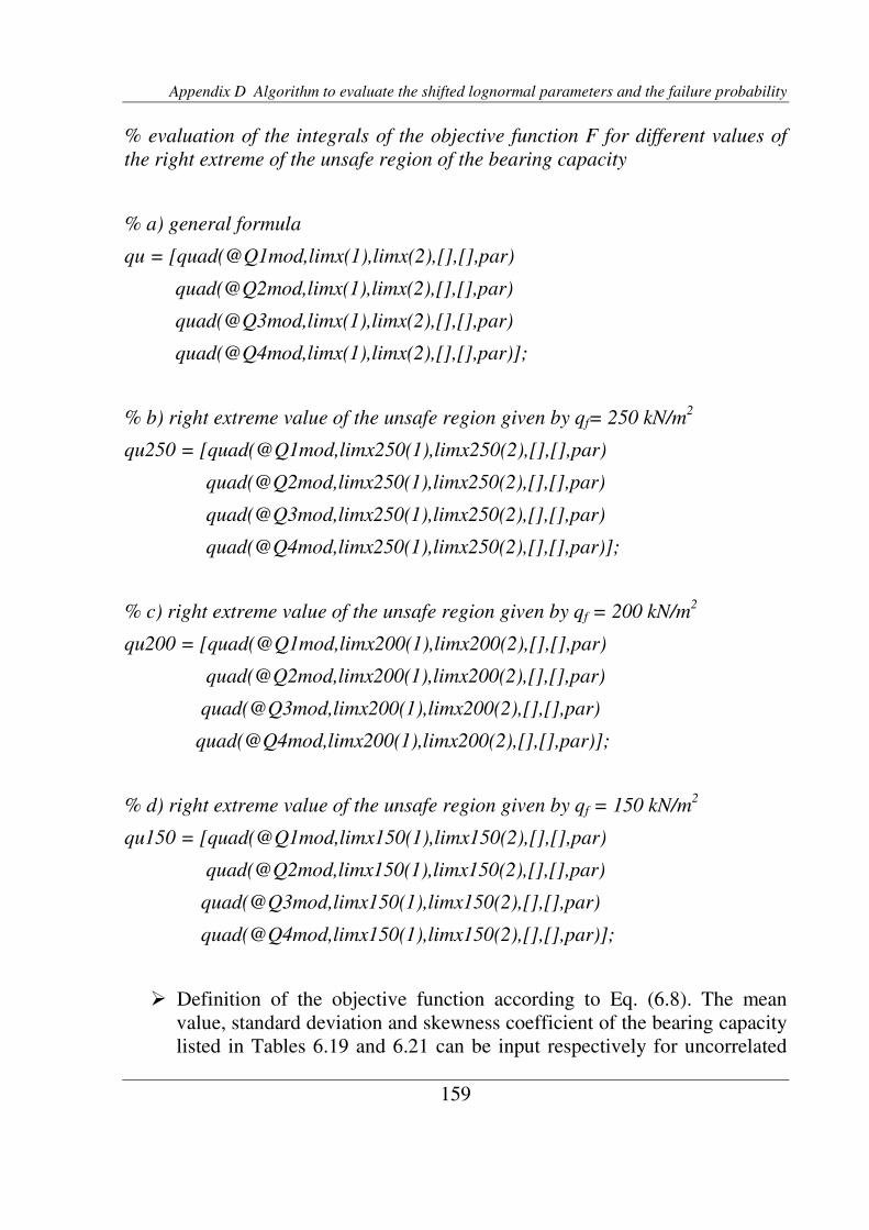
Appendix D Algorithm to evaluate the shifted lognormal parameters and the failure probability
159
% evaluation of the integrals of the objective function F for different values of
the right extreme of the unsafe region of the bearing capacity
% a) general formula
qu = [quad(@Q1mod,limx(1),limx(2),[],[],par)
quad(@Q2mod,limx(1),limx(2),[],[],par)
quad(@Q3mod,limx(1),limx(2),[],[],par)
quad(@Q4mod,limx(1),limx(2),[],[],par)];
% b) right extreme value of the unsafe region given by qf= 250 kN/m2
qu250 = [quad(@Q1mod,limx250(1),limx250(2),[],[],par)
quad(@Q2mod,limx250(1),limx250(2),[],[],par)
quad(@Q3mod,limx250(1),limx250(2),[],[],par)
quad(@Q4mod,limx250(1),limx250(2),[],[],par)];
% c) right extreme value of the unsafe region given by qf = 200 kN/m2
qu200 = [quad(@Q1mod,limx200(1),limx200(2),[],[],par)
quad(@Q2mod,limx200(1),limx200(2),[],[],par)
quad(@Q3mod,limx200(1),limx200(2),[],[],par)
quad(@Q4mod,limx200(1),limx200(2),[],[],par)];
% d) right extreme value of the unsafe region given by qf = 150 kN/m2
qu150 = [quad(@Q1mod,limx150(1),limx150(2),[],[],par)
quad(@Q2mod,limx150(1),limx150(2),[],[],par)
quad(@Q3mod,limx150(1),limx150(2),[],[],par)
quad(@Q4mod,limx150(1),limx150(2),[],[],par)];
Definition of the objective function according to Eq. (6.8). The mean
value, standard deviation and skewness coefficient of the bearing capacity
listed in Tables 6.19 and 6.21 can be input respectively for uncorrelated
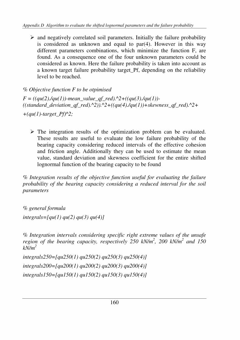
Appendix D Algorithm to evaluate the shifted lognormal parameters and the failure probability
160
and negatively correlated soil parameters. Initially the failure probability
is considered as unknown and equal to par(4). However in this way
different parameters combinations, which minimize the function F, are
found. As a consequence one of the four unknown parameters could be
considered as known. Here the failure probability is taken into account as
a known target failure probability target_Pf, depending on the reliability
level to be reached.
% Objective function F to be otpimised
F = ((qu(2)./qu(1))-mean_value_qf_red).^2+((qu(3)./qu(1))-
((standard_deviation_qf_red).^2)).^2+((qu(4)./qu(1))+skewness_qf_red).^2+
+(qu(1)-target_Pf)^2;
The integration results of the optimization problem can be evaluated.
These results are useful to evaluate the low failure probability of the
bearing capacity considering reduced intervals of the effective cohesion
and friction angle. Additionally they can be used to estimate the mean
value, standard deviation and skewness coefficient for the entire shifted
lognormal function of the bearing capacity to be found
% Integration results of the objective function useful for evaluating the failure
probability of the bearing capacity considering a reduced interval for the soil
parameters
% general formula
integrals=[qu(1) qu(2) qu(3) qu(4)]
% Integration intervals considering specific right extreme values of the unsafe
region of the bearing capacity, respectively 250 kN/m2, 200 kN/m
2 and 150
kN/m2
integrals250=[qu250(1) qu250(2) qu250(3) qu250(4)]
integrals200=[qu200(1) qu200(2) qu200(3) qu200(4)]
integrals150=[qu150(1) qu150(2) qu150(3) qu150(4)]

Appendix D Algorithm to evaluate the shifted lognormal parameters and the failure probability
161
D.3 Subroutines for the definition of the integrals of the objective function
Using the following subroutines it is possible to define the integrals of the
optimization function F to be estimated.
1) Subroutine for defining the integral of the failure probability Pf, where
f1=fX(x). The function fX(x) is the probability density function of the shifted
lognormal function:
function f1 =Q1mod(x,par)
f1 = (1./(((2*pi)^0.5).*(par(2)).*(x-par(3)))).*(exp(-0.5.*(((log(x-par(3))-
par(1))./(par(2))).^2))) ;
2) Subroutine for defining the integral of the mean value µqfred, where
f2=x*fX(x):
function f2 =Q2mod(x,par)
f2 = x.*((1./(((2*pi)^0.5).*(par(2)).*(x-par(3)))).*(exp(-0.5.*(((log(x-par(3))-
par(1)).//(par(2))).^2))));
3) Subroutine for defining the integral of the variance σqfred2, knowing the mean
value µqfred from the subroutine 2). The function f3 corresponds to (x-
µqfred)2*fX(x):
function f3 =Q3mod(x,par)
f3 = ((x-µqfred).^2).*((1./(((2*pi)^0.5).*(par(2)).*(x-par(3)))).*(exp(-0.5.
*(((log(x-par(3))-par(1))./(par(2))).^2))));
4) Subroutine for defining the integral of the skewness coefficient νqfred,
knowing the mean value µqfred and the variance σqfred2 respectively from
subroutine 2) and 3). The function f4 corresponds to (x-µqfred)3*fX(x)/ σqfred
3:
function f4 =Q4mod(x,par)
f4 = (((x-µqfred )./(σqfred)).^3).*((1./(((2*pi)^0.5).*(par(2)).*(x-par(3)))).*(exp(-
0.5.*(((log(x-par(3))-par(1))./(par(2))).^2))));

Appendix D Algorithm to evaluate the shifted lognormal parameters and the failure probability
162
D.4 Optimisation results for the bearing capacity problem
D.4.1 Case with ρρρρc´tanϕϕϕϕ´ = 0
The results of the optimization problem previously described considering the
bearing capacity results of Table 6.19 and the failure probability as known are
listed above:
- the parameters of the shifted lognormal distribution
m = 5.905 kN/m2
s = 0.233 kN/m2
u = -95.868 kN/m2
- the low failure probability of the bearing capacity considering as right extreme
value of the unsafe region, respectively, 150 kN/m2, 200 kN/m
2 and 250 kN/m
2
Pf150 = 0.043
Pf200 = 0.0437
Pf250 = 0.0463
- the extreme values of the integration interval of the objective function
x0 = -95.768 kN/m2
xm = 140.477 kN/m2
- the statistical values of the entire shifted lognormal distribution of the bearing
capacity
mean_value = 280.954 kN/m2
standard_deviation = 10.392 kN/m2
skewness = 0.083
- the minimum value of the objective function
Feval = 0.00005
Appendix D Algorithm to evaluate the shifted lognormal parameters and the failure probability
163
D.4.2 Case with ρρρρc´tanϕϕϕϕ´ = -0.6
For the bearing capacity results of Table 6.21 the optimization problem earlier
described leads to the following results, considering the failure probability as
known:
- the parameters of the shifted lognormal distribution
m = 5.478 kN/m2
s = 0.251 kN/m2
u = 36.456 kN/m2
- the low failure probability of the bearing capacity considering as right extreme
value of the unsafe region, respectively, 150 kN/m2, 200 kN/m
2 and 250 kN/m
2
Pf150 = 0.0015
Pf200 = 0.0016
Pf250 = 0.0029
- the extreme values of the integration interval of the objective function
x0 = 36.556 kN/m2
xm = 141.814 kN/m2
- the statistical values of the entire shifted lognormal distribution of the bearing
capacity
mean_value = 283.629 kN/m2
standard_deviation = 7.941 kN/m2
skewness = 0.096
- the minimum value of the objective function
Feval = 1.524

165
Bibliography
ANG, A.H.-S.; TANG, W.H. (1975): “Probability Concepts in Engineering
Planning and Design, Vol. I: Basic Principles”. John Wiley and Sons, New
York.
ANG, A.H.-S.; TANG, W.H. (1984): “Probability Concepts in Engineering
Planning and Design, Vol. II: Decision, Risk and reliability”. John Wiley and
Sons, New York.
ANG, A.H.-S.; TANG, W.H. (2006): “Probability Concepts in Engineering.
Emphasis on Applications to Civil and Environmental Engineering”. 2nd
Edition, John Wiley and Sons, New York.
BAECHER, G. B. (1982): “Statistical methods in site characterization”.
Updating subsurface
samplings of soils and rocks and their in-situ testing, Engineering Foundation,
Santa Barbara, California, pp. 463-492.
BENJAMIN, J.R.; CORNELL, C.A. (1970): “Probability, statistics and decision
making for civil engineers”. McGraw Hill, London, New York.
BRINCH HANSEN, J. (1961): “A general formula for bearing capacity”.
Danisch Geotechnical Institute, Bulletin 11.
BÜCHTER, A.; HENN, H.-W. (2000): “Elementare Stochastik. Eine
Einführung in die Mathematik der Daten und des Zufalls”. Mathematik für das
Lehramt. Springer, Berlin.
CAQUOT, A.; KERISEL, J. (1953): “Sur le terme de surface dans le calcul des
fondations en milieu pulverulent“. 3th ICSMFE, Rotterdam, Vol. 1: pp. 265-
270.

Bibliography
166
CHERUBINI, C. (1997): “Data and considerations on the variability of
geotechnical properties of soils”. Proceedings of the International Conference
on Safety and Reliability (ESREL) 97, Lisbon, Vol. 2: pp. 1583-1591.
CHERUBINI, C. (1998): “Reliability of shallow foundation bearing capacity on
c´, ϕ´ soils”. Canadian Geotechnical Journal, Vol. 37: pp. 264-269.
CHOWDHURY, R.N. (1984): “Recent developments in landslide studies:
Probabilistic methods, State-of-the-art-report – Session VII(a)”. International
Symposium on Landlside, pp. 209-228.
CHRISTIAN, J.T. (2004): “Geotechnical Engineering Reliability: How Well do
we know what we are doing?”. Journal of Geotechnical and
Geoenvironmental Engineering, Vol. 130(10): pp. 985-1003.
CHRISTIAN, J.T.; LADD, C.C.; BAECHER, G.B. (1992): “Reliability Applied
to Slope Stability Analysis”. Journal of Geotechnical Engineering, Vol. 120:
pp. 2180-2207.
CHRISTIAN, J.T.; LADD, C.C.; BAECHER, G.B. (1994): “Reliability and
Probability in Stability Analysis”. Stability and Performance of Slopes and
Embankments II (Geotechnical Special Publication): pp. 1071-1111.
CHRISTIAN, J.T.; BAECHER, G.B. (1999): “Point Estimate Method as
Numerical Quadrature”. Journal of Geotechnical and Geoenvironmental
Engineering: pp. 779-786.
CHRISTIAN, J.T.; BAECHER, G.B. (2002): “The point estimate method with
large numbers
of variables”. International Journal for Numerical and Analytical Methods in
Geomechanics, Vol. 26: pp. 1515-1529.
CORNELL, C.A. (1969): “A probability-based structural code”. Journal of the
American
Concrete Institute, Vol. 66: pp. 974-985.
DAS, B.J. (1996): “Principles of Geotechnical Engineering“. California State
University, Sacramento.
Bibliography
167
DITLEVSEN, O.; MADSEN, H. O. (1996): “Structural reliability methods“.
Chichester: John Wiley & Sons.
DUNCAN, J.M. (2000): “Factors of Safety and reliability in geotechnical
engineering”. Journal of Geotechnical and Geoenvironmental Engineering,
Vol. 126: pp. 307-316.
EINSTEIN, H. H.; BAECHER, G. B.(1982): “Probabilistic and statistical
methods in
engineering geology. I. Problem statement and introduction to solution”. Rock
Mechanics, Supp. 12, pp. 47-61.
EL-RAMLY, H.; MORGENSTERN, N.R.; CRUDEN, D.M. (2001):
“Probabilistic Slope Stability Analysis for Practice”. Canadian Geotechnical
Journal, Vol. 40: pp. 851-855.
EL-RAMLY, H.; MORGENSTERN, N.R.; CRUDEN, D.M. (2003): Reply to
the discussion by J.M. Duncan, M. Navin, and T.F. Wolff on “Probabilistic
Slope Stability Anaylsis for Practice”. Canadian Geotechnical Journal, Vol.
39: pp. 665-683.
EL-RAMLY, H.; MORGENSTERN, N.R.; CRUDEN, D.M. (2005):
“Probabilistic assessment of stability of a cut slope in residual soil”.
Géotechnique, 55: 77-84.
EUROCODE 7 (1994): “ENV 1997-1 Geotechnical design, general rules”.
Delft: CEN European Committee for Standardisation.
EVANS, M.; HASTINGS, N.; PEACOCK, B. (1993): “Statistical distributions”.
Wiley, New York.
FENTON, G.A. (2006): “Basics of Simulation”. Proceedings of the CISM-
Meeting “Probabilistic Methods in Geotechnical Engineering”, Udine.
FENTON, G.A.; GRIFFITHS, D.V. (2003): “Bearing Capacity Prediction of
Spatially Random c-ϕ soils”. Canadian Geotechnical Journal, Vol. 40: pp. 54-
65.
Bibliography
168
FENTON, G.A.; GRIFFITHS, D.V. (2004): “Reply to the discussion by R.
Popescu on “Bearing Capacity Prediction of Spatially Random c-ϕ soils””.
Canadian Geotechnical Journal, Vol. 41: pp. 368-369.
GRIFFITHS, D.V.; FENTON, G.A.; TVETEN, D.E. (2002): “Probabilistic
Geotechnical Analysis: how difficult does it need to be?”. International
Conference on Probabilistics in Geotechnics, pp. 3-20.
GRIFFITHS, D.V.; FENTON, G.A.; MANOHARAN, N. (2002): “Bearing
Capacity of Rough Rigid Strip Footing on Cohesive Soil: Probabilistic study”.
Journal of Geotechnical and Geoenvironmental Engineering, Vol. 128: pp.
743-755.
HARR, M. T. (1989): “Probabilistic estimates for multivariate analyses“. Appl.
Math. Modelling, Vol. 13(5): pp. 313-318.
HARR, M. E. (1996): “Reliability-based design in civil engineering“. Dover
publications, Inc., Mineola, New York.
HASOFER, A. M.; LIND, N. (1974): “Exact and Invariant Second-Moment
Code Format“.
Journal of Engineering Mechanics, Vol. 100(1): pp. 111-121.
HONG, H. P. (1998): “An efficient point estimate method for probabilistic
analysis“. Reliability Engineering and System Safety, Vol. 59(3): pp. 261-267.
HONJO, Y.; AMATYA, S. (2005): “Partial factors calibration based on
reliability analyses for square footings on granular soils“. Géotechnique, Vol.
6: pp. 479-491.
KATZENBACH, R.; MOORMANN, C. (2003): “Überlegungen zu
stochastischen Methoden in der Bodenmechanik am Beispiel des Frankfurter
Tons“. Beiträge anlässlich des 60. Geburtstages von Herrn Prof. Dr. S.
Semprich, Heft 16 der Gruppe Geotechnik, Technische Universität Graz: pp.
255-282.
KENNEY, J. F.; KEEPING, E. S. (1951): “Mathematics of Statistics“. Pt. 2, 2nd
Ed., Princeton, NJ: Van Nostrand.
Bibliography
169
KOTTEGODA, N. T.; ROSSO, R. (1997): “Statistics, Probability and
Reliability for Civil and Environmental Engineers”. The McGraw-Hill
Companies, Inc, USA.
KULHAWY; F. H. (1992): “On evaluation of static soil properties”. In Stability
and performance of slopes and embankments II (GPS 31), American Society
of Civil Engineers, Seed, R. B., Boulanger, R. W., eds, pp. 95-115.
LACASSE, S.; NADIM, F. (1996): “Uncertainties in Characterizing Soil
Properties”. In Uncertainty in the Geologic Environment: from Theory to
Practice, Proceedings of Uncertainty ´96, ASCE Geotechnical Special
publication No. 58, C.D. Shackelford, P.P. Nelson, M.J.S. Roth, eds., pp. 49-
75.
LADD, C. C.; DASCAL; O.; LAW, K.T.; LEFEBRVE, G.; LESSARD, G.;
MESRI, G.; TAVENAS, F. (1983): Report of the subcommittee on
embankment stability – annex II. Committee of Specialists on Sensitive Clays
on the NBR Complex, Société d´Energie de la Baie James, Montréal, Quebec.
LANCELLOTTA, R. (1993): “Geotechnical Engineering”. Mc Graw-Hill.
LANCELLOTTA, R.; CALAVERA, J. (1999): “Fondazioni”. McGraw-Hill.
LI, K.S. (1992): “Point-estimate method for calculating statistical moments”.
Journal of Engineering Mechanics, ASCE 118(7): pp. 1506-1511.
LI, K.S.; LUMB, P. (1987): “Probabilistic design of slopes”. Canadian
Geotechnical Journal, Vol. 24: pp. 520-535.
LI, K.S.; WHITE, W. (1987): “Probabilistic Approaches to Slope Design”.
Research Report No. 20, Civil Engineering Department, Australian Defence
Force Academy, Canberra, Australia, pp. 54.
LIND, N.C. (1983): “Modelling uncertainty in discrete dynamical systems”.
Applied Mathematical Modelling, Vol. 7(3): pp. 146-152.
LUMB, P. (1969): “Safety factors and the probability distribution of soil
strength”. Canadian Geotechnical Journal, Vol. 7(3): pp. 225-242.

Bibliography
170
MEYERHOF, G. G. (1963): “Some recent research on the bearing capacity of
foundations”. Canadian Geotechnical Journal, Vol. 1: pp. 16-26.
MOSTYN, G.R.; LI, K.S. (1993): “Probabilistic Slope Analysis-State of Play”.
Probabilistic Methods in geotechnical Engineering, eds Li & Lo, pp. 89-109.
NATIONAL RESEARCH COUNCIL REPORT (1995): “Appendix A: Basic
Concepts of Probability and Reliability”. Probabilistic Methods in
Geotechnical Engineering.
NADIM, F. (2006): “First Order Second Moment (FOSM), First and Second
Order Reliability Methods (FORM & SORM), Monte Carlo Simulation,
System Reliability”. Proceedings of the CISM Course “Probabilistic methods
in geotechnical engineering”, Udine.
PESCHL, G. M. (2004): “Reliability analysis in geotechnics with the random set
finite element method”. Heft 25 des Institutes für Bodenmechanik und
Grundbau, Technische Universität Graz.
PHOON, K.-K.; KULHAWY, F.H. (1994): “Characterization of Geotechnical
Variability”. Canadian Geotechnical Journal, Vol. 36: pp. 612-624.
PHOON, K.-K.; KULHAWY, F.H. (1999): “Evaluation of geotechnical
property variability”. Canadian Geotechnical Journal, Vol. 36: pp. 625-639.
POPESCU, R. (2004): “Discussion of Bearing Capacity Prediction of Spatially
Random c-ϕ soils”. Canadian Geotechnical Journal, Vol. 41: pp. 366-367.
PÖTTLER, R.; KLAPPERICH, H.; SCHWEIGER, H.F. (2002): “International
Conference on Probabilistics in Geotechnics. Technical and Economic Risk
estimation“.
PRANDTL, L. (1921): “Eindringungsfestigkeit und Festigkeit von Schneiden“.
Zeitung für angewendete Mathematik und Mechanik, Vol. 1:15.
PULA, W. (2006): “FORM/SORM applications in bearing capacity problems”.
Proceedings of the CISM Course “Probabilistic methods in geotechnical
engineering”, Udine.
RÉTHÁTI, L. (1987): “Probabilistic Solutions in Geotechnics”.

Bibliography
171
ROSENBLATT, M. (1952): “Remarks on a Multivariate Transformation”.
Annals of Math.
Stat., Vol. 23(3): pp.470-472.
ROSENBLUETH, E. (1975): “Point estimates for probability moments”. Proc.
Nat. Acad. Sci. USA, Vol. 72 (10): pp. 3812-3814.
ROSENBLUETH, E. (1981): “Two-point estimates in probabilities”. Appl.
Math. Modelling, Vol. 5(2): pp. 329-335.
ROSSI, F.; SALVI, F. (2001): “Manuale di Ingegneria Civile. Vol. I:
Matematica, Idraulica, Ingegneria Geotecnica, Costruzioni idrauliche”.
Zanichelli, ESAC.
ROSS, S. M. (1995): “A course in simulation”. Macmillan, New York.
RUSSELLI, C.; VERMEER, P. A. (2005): “Probabilistic Methods applied to
Geotechnical Engineering”. Proceedings of the 2nd International Workshop of
Young Doctors in Geomechanics (WHYDOC), Ecole Nationale des Ponts et
Chaussées (ENPC), Champs-sur-Marne, France, pp. 361-366.
RUSSELLI, C.; VERMEER, P. A. (2006): “Wahrscheinlichkeitsmethoden
angewendet auf geotechnische Probleme“. Tagungshandbuch des 5.
Kolloquiums "Bauen in Boden und Fels", Technische Akademie Esslingen
(TAE), Esslingen, pp. 183-186.
SCHAD, H.; WALLRAUCH, E. (1985): “Rutschungen im Keuper“. Otto-Graf
Institut (MPA), Universität Stuttgart.
SCHNEIDER, J.; SCHLATTER, H.P. (1996): “Sicherheit und Zuverlässigkeit
im Bauwesen. Grundwissen für Ingenieure“. Hochschulverlag AG an der ETH
Zürich & B.G. Teubner Stuttgart.
SCHWEIGER; H.F.; THURNER, R.; PÖTTLER, R. (2001): “Reliability
Anaylsis in Geotechnics with Deterministic Finite Elements. Theoretical
Concepts and Practical Application“. The International Journal of
Geomechanics, Vol. 1: 389-413.

Bibliography
172
SHOOMAN; M.L. (1968): “Probabilistic Reliability: An Engineering
Approach”. McGraw-Hill Book Co., New York.
SPEEDIE, M. G. (1956): “Selection of Design Value from Shear Test Results“.
Proceedings of the 2nd
Australia-New Zealand Conference on Soil Mechanics
and Foundation Engineering, Wellington, pp. 107-109.
TERZAGHI, K. (1943): “Theoretical Soil Mechanics”. Whiley, New York.
THURNER, R. (2000): “Probabilistische Untersuchungen in der Geotechnik
mittels
deterministischer Finite Elemente-Methode”. Dissertation eingereicht an der
Fakultät für Bauingenieurwesen der Technischen Universität Graz.
TOBUTT, D. C. (1981): “Monte Carlo Simulation Methods for Slope Stability”.
Computers & Geosciences, Vol. 8(2): pp. 199-208.
TUNG, Y-K. (1998): “Uncertainty and Reliability Analysis in Water Resources
Engineering”. Department of Civil & Structural Engineering, Hong Kong
University of Science & Technology.
U.S. Army Corps of Engineers (1995): “Introduction to Probability and
Reliability in Geotechnical Engineering”. Appendix B to ETL 1110-2-547.
VANMARCKE, E.H. (1980): “Probabilistic stability analysis of earth slopes”.
Engineering Geology, Vol. 16: pp. 29-50.
VaP (Variables Processor) 2.2 - User manual (2006). PSP-Petschacher Software
und
Entwicklungs GmbH.
VRIJLING, J.K. (1997): “Probabilities in civil engineering, Part 1: Probabilistic
design in theory”. CUR-Publicatie 190, Delft University of Technology,
Stichting CUR, Gouda.
WHITMAN, R.V. (1984): “Evaluating the calculated risk in geotechnical
engineering”. Journal of Geotechnical Engineering, ASCE, Vol. 110(2): pp.
145-188.

Bibliography
173
WOLFF, T.F.; SHANNON; WILSON (1999): “An Overview of Probabilistic
Analysis for Geotechnical Engineering Problems”. Appendix A to U.S. Army
Corps of Engineers: Circular Risk-Based Analysis in Geotechnical
Engineering for Support of Planning Studies, ETL 1110-2-556.
WOLFF, T.F. (1994): “Evaluating the Reliability of Existing Levees”. Research
report prepared for U.S. Army Waterways Experiment Station, Michigan State
University.
ZHOU, J.; NOWAK, A.S. (1988): “Integration formulas to evaluate functions of
random variables”. Structural safety, Vol. 5: pp. 267-284.


175
Curriculum Vitae
09.01.1977
Born in Venaria Reale, Turin, Italy
1996 – 2000
Study in Civil Engineering at the Polytechnic University of Turin
2000 – 2001
Study in Civil Engineering at the “Institut National des Sciences
Appliquées” (INSA), Lyon
08. – 11.2001
Internship at the TNO Building and Construction Research, Delft
19.03.2002
Diploma graduation at the Polytechnic University of Turin
07. – 09.2002
Research Associate at the Institute of Automative Engineering and
Vehicle Engines (FKFS), University of Stuttgart
10.2002 – 09.2003
Research Associate at the MPA Otto-Graf-Institute, University of Stuttgart
10.2003 – 10.2006
Doctoral study; Research and Teaching Assistant at the Institute of
Geotechnical Engineering, University of Stuttgart
since 02.2007
Research Assistant at the MPA Otto-Graf-Institute, University of
Stuttgart
14.02.2008
Doctoral exam

Mitteilungen des Instituts für Geotechnik
Nr. 01 Thamm, B. R. (1974) Anfangssetzungen und Anfangsporenwasser-
überdrücke eines normalverdichteten wasser-
gesättigten Tones
€ 5,11
Nr. 02 Gußmann, P. (1975) Einheitliche Berechnung von Grundbruch und
Böschungsbruch
€ 2,56
Nr. 03 Feeser, V. (1975) Die Bedeutung des Kalziumkarbonats für die
bodenphysikalischen Eigenschaften vom Löß
vergriffen
Nr. 04 Du Thin, K. (1976) Standsicherheit von Böschungen: Programm-
Dokumentation
vergriffen
Nr. 05 Smoltczyk, U./
Pertschi, O./
Hilmer, K.
(1976) Messungen an Schleusen in der UDSSR.
Schleusennorm der UDSSR (SN 30365)
vergriffen
Nr. 06 Hilmer, K. (1976) Erddruck auf Schleusenkammerwände
€ 9,20
Nr. 07 Laumans, Q. (1977) Verhalten einer ebenen, in Sand eingespannten
Wand bei nichtlinearen Stoffeigenschaften des
Bodens
€ 9,20
Nr. 08 Lächler, W. (1977) Beitrag zum Problem der Teilflächenpressung
bei Beton am Beispiel der Pfahlkopfanschlüsse
vergriffen
Nr. 09 Spotka, H. (1977) Einfluß der Bodenverdichtung mittels Ober-
flächenrüttelgeräten auf den Erddruck einer
Stützwand bei Sand
vergriffen
Nr. 10 Schad, H. (1979) Nichtlineare Stoffgleichungen für Böden und
ihre Verwendung bei der numerischen Analyse
von Grundbauaufgaben
vergriffen

Nr. 11 Ulrich, G.
Gußmann, P.
(1980) Verschiebungs- und kraftgesteuerte Platten-
druckversuche auf konsolidierenden Böden
Zum Modellgesetz der Konsolidation
€ 10,23
Nr. 12 Salden, D. (1980) Der Einfluß der Sohlenform auf die Traglast
von Fundamenten
€ 12,78
Nr. 13 Seeger, H. (1980) Beitrag zur Ermittlung des horizontalen
Bettungsmoduls von Böden durch
Seitendruck-versuche im Bohrloch
€ 12,78
Nr. 14 Schmidt, H.H. (1981) Beitrag zur Ermittlung des Erddrucks auf
Stützwände bei nachgiebigem Baugrund
€ 12,78
Nr. 15 Smoltczyk, U./
Schweikert, O.
(1981) Vorstudie über bauliche Alternativen für
Durch-gangsstraßen in Siedlungen
€ 6,14
Nr. 16 Malcharek, K./
Smoltczyk, U.
(1981) Vergleich nationaler Richtlinien für die
Berech-nung von Fundamenten
€ 7,67
Nr. 17 Gruhle, H.D. (1981) Das Verhalten des Baugrundes unter
Einwirkung vertikal gezogener Ankerplatten
als räumliches Problem des Erdwiderstandes
vergriffen
Nr. 18 Kobler, W. (1982) Untersuchungen über Böschungs- und Grund-
bruch bei begrenzten Lastflächen
€ 12,78
Nr. 19 Lutz, W. (1983) Tragfähigkeit des geschlitzten Baugrunds
neben Linienlasten
€ 12,78
Nr. 20 Smoltczyk, U. (1983) Studienunterlagen “Bodenmechanik und
Grund-bau“; überarbeitete Ausgabe 1993
€ 20,45

Nr. 21 Schweikert, O. (1984) Der Einfluß des Böschungswinkels auf die Be-
rechnung des aktiven Erddrucks
€ 10,23
Nr. 22 Vogt, N. (1984) Erdwiderstandsermittlung bei monotonen und
wiederholten Wandbewegungen in Sand
vergriffen
Nr. 23 Buchmaier, R. (1985) Zur Berechnung von Konsolidationsproblemen
bei nichtlinearem Stoffverhalten
€ 12,78
Nr. 24 Schad, H.
Smoltczyk, U./
Schad, H./
Zoller, P.
(1985) Möglichkeiten der Böschungssicherung bei
kleinen Baugruben
Sonderkonstruktionen der Böschungssicherung
€ 17,90
Nr. 25 Gußmann, P. (1986) Die Methode der Kinematischen Elemente
€ 10,23
Nr. 26 Steinmann, B. (1985) Zum Verhalten bindiger Böden bei monotoner
einaxialer Beanspruchung
vergriffen
Nr. 27 Lee, S.D. (1987) Untersuchungen zur Standsicherheit von
Schlit-zen im Sand neben Einzelfundamenten
vergriffen
Nr. 28 Kolb, H. (1988) Ermittlung der Sohlreibung von
Gründungskör-pern unter horizontalem
kinematischen Zwang
€ 12,78
Nr. 29 Ochmann, H. (1988) Ebene Grenzzustände von Erdböschungen im
stochastischen Sicherheitskonzept
€ 12,78
Nr. 30 Breinlinger, F. (1989) Bodenmechanische Stoffgleichungen bei
großen Deformationen sowie Be- und
Entlastungsvor-gängen
€ 15,34
Nr. 31 Smoltczyk, U./
Breilinger, F./
Schad, H./
Wittlinger, M.
(1989) Beitrag zur Bemessung von Tunneln in offener
Bauweise
€ 12,78
Nr. 32 Gußmann, P./
Schanz, T./
Smoltczyk, U./
Willand, E.
(1990) Beiträge zur Anwendung der KEM (Erddruck,
Grundbuch, Standsicherheit von Böschungen)
vergriffen
Nr. 33 Gruhle, H.D. (1990) Der räumliche Erdwiderstand vor überwiegend
horizontal belasteten Ankerplatten
vergriffen
Nr. 34 Henne, J. (1995) Zur Bewehrung von verformten
Bodenschichten durch Einsatz zugfester
Geokunststoffe
€ 15.34
Nr. 35 Wittlinger, M. (1994) Ebene Verformungsuntersuchungen zur We-
ckung des Erdwiderstandes bindiger Böden
€ 15,34
Nr. 36 Schad, H.
(1992) Zeit- und geschwindigkeitsabhängiges Materi-
alverhalten in der Geotechnik - Experimentelle
Erfassung und numerische Analyse
€ 15,34
Nr. 37 Belz, I. (1992) Zur Ermittlung dynamischer Bodenkennwerte
in situ aus der Systemantwort des Erregers
€ 15,34
Nr. 38 Ma, J. (1994) Untersuchungen zur Standsicherheit der durch
Stützscheiben stabilisierten Böschungen
€ 15.34
Nr. 39 Smoltczyk, U. (1994) Sonderheft: 25 Jahre Lehre und Forschung in
der Geotechnik
€ 15.34
Nr. 40 Rilling, B. (1994) Untersuchungen zur Grenztragfähigkeit bindi-
ger Schüttstoffe am Beispiel von Lößlehm
€ 17.90
Nr. 41 Vermeer, P.A. (1996) Deponiebau und Geotechnik
€ 17,90
Nr. 42 Vermeer, P.A. (1997) Baugruben in Locker- und Festgestein
€ 17,90
Nr. 43 Brinkmann, C. (1998) Untersuchungen zum Verhalten von
Dichtungs-übergängen im Staudammbau
€ 17,90
Nr. 44 Fiechter-
Scharr, I.
(1998) Beeinflussung von Erdbaustoffen durch
Beimi-schen eines organophilen Bentonits
€ 17,90
Nr. 45 Schanz, T. (1998) Zur Modellierung des mechanischen
Verhaltens von Reibungsmaterialien
€ 17,90
Nr. 46 Akinrogunde,
A.E.
(1999) Propagation of Cement Grout in Rock Discon-
tinuities Under Injection Conditions
€ 17,90
Nr. 47 Vogt-Breyer,
C.
(1999) Experimentelle und numerische
Untersuchungen zum Tragverhalten und zur
Bemessung hori-zontaler Schraubanker
€ 17,90
Nr. 48 Vermeer, P.A. (1999) Neue Entwicklungen in der Geotechnik
€ 17,90
Nr. 49 Marcher, T. (2002) Resultate eines Versuchsprogramms an Beau-
caire Mergel
€ 17,90
Nr. 50 Marcher, T. (2003) Nichtlokale Modellierung der Entfestigung
dichter Sande und steifer Tone
€ 17,90
Nr. 51 Ruse, N.M. (2004) Räumliche Betrachtung der Standsicherheit
der Ortsbrust beim Tunnelvortrieb
€ 17,90
Nr. 52 Beutinger, P.H. (2005) Ein geotechnischer Beitrag zur Standsicherheit
mobiler Baumaschinen
€ 17,90

Nr. 53 Wehnert, M. (2006) Ein Beitrag zur drainierten und undrainierten
Analyse in der Geotechnik
€ 17,90
Nr. 54 Möller, S. C. (2006) Tunnel induced settlements and forces in
linings
€ 17,90
Nr. 55 Benz, T. (2007) Small-Strain Stiffness of Soils and its
Numerical Consequences
€ 17,90
Nr. 56 Abed, A. (2008) Numerical Modeling of Expansive Soil
Behavior
€ 17,90
Nr. 57 Hintner, J. (2008) Analyse der Fundamentverschiebungen
infolge vertikaler und geneigter Belastung
€ 17,90
Nr. 58 Russelli, C. (2008) Probabilistic Methods applied to the Bearing
Capacity Problem
€ 17,90