probabilistic methods in telecommunication

PROBABILISTIC METHODS

IN TELECOMMUNICATION

Benedikt Jahnel

WIAS Berlin

and

Wolfgang Konig

TU Berlin and WIAS Berlin

Lecture Notes

7 June, 2018

Contents

1 Device locations: Poisson point processes 3

1.1 Point processes . . . . . . . . . . . . . . . . . . . . . . . . . . . . . . . . . . . . . 3

1.2 Definition and first properties of the Poisson point process . . . . . . . . . . . . . 6

1.3 The Campbell moment formulas . . . . . . . . . . . . . . . . . . . . . . . . . . . 10

1.4 Marked Poisson point processes . . . . . . . . . . . . . . . . . . . . . . . . . . . . 11

1.5 Conditioning: the Palm version . . . . . . . . . . . . . . . . . . . . . . . . . . . . 13

1.6 Random intensity measures: Cox point processes . . . . . . . . . . . . . . . . . . 15

1.7 Convergence of point processes . . . . . . . . . . . . . . . . . . . . . . . . . . . . 19

2 Coverage and connectivity: the Boolean model 23

2.1 The Boolean model . . . . . . . . . . . . . . . . . . . . . . . . . . . . . . . . . . . 24

2.2 Coverage properties . . . . . . . . . . . . . . . . . . . . . . . . . . . . . . . . . . 24

2.3 Long-range connectivity in the homogeneous Boolean model . . . . . . . . . . . . 27

2.4 Intermezzo: phase transition in discrete percolation . . . . . . . . . . . . . . . . . 29

2.5 Proof of phase transition in continuum percolation . . . . . . . . . . . . . . . . . 32

2.6 More about the percolation probability . . . . . . . . . . . . . . . . . . . . . . . . 33

2.7 Percolation for Cox point processes . . . . . . . . . . . . . . . . . . . . . . . . . . 37

3 Interference: the signal-to-interference ratio 39

3.1 Describing interference . . . . . . . . . . . . . . . . . . . . . . . . . . . . . . . . . 39

3.2 The signal-to-interference ratio . . . . . . . . . . . . . . . . . . . . . . . . . . . . 42

3.3 SINR percolation . . . . . . . . . . . . . . . . . . . . . . . . . . . . . . . . . . . . 44

4 Events of bad quality of service: large deviations 47

4.1 Introductory example . . . . . . . . . . . . . . . . . . . . . . . . . . . . . . . . . 47

4.2 Principles of large deviations . . . . . . . . . . . . . . . . . . . . . . . . . . . . . 49

4.3 LDP in the high-density setting . . . . . . . . . . . . . . . . . . . . . . . . . . . . 50

4.4 An application to user connectivity . . . . . . . . . . . . . . . . . . . . . . . . . . 51

5 Random malware propagation: the contact process 55

5.1 Markov chains in continuous time . . . . . . . . . . . . . . . . . . . . . . . . . . . 56

i

ii CONTENTS

5.2 The contact process . . . . . . . . . . . . . . . . . . . . . . . . . . . . . . . . . . 57

5.3 The contact process on Zd . . . . . . . . . . . . . . . . . . . . . . . . . . . . . . . 58

5.4 Other IPS for telecommunications . . . . . . . . . . . . . . . . . . . . . . . . . . 59

References 61

Index 63

Preface

These are the lecture notes for a two-hours lecture, held by us in the summer semester 2018at Technische Universitat Berlin. We introduce mathematical concepts and theories for therigorous probabilistic analysis of a certain type of a telecommunication system, an multi-hop adhoc system. Such a system consists of users, base stations and message trajectories, jumping inseveral hops from user to user and/or base station. The term ad hoc expresses the fact that themessages do not have to jump to a base station directly and from there to their targets, but theyuse all the users present in the system for a sequence of hops to reach the target. Such a systemhas some advantages over systems that require direct hops to base stations: it does not need tohave many (expensive!) base stations and can potentially absorb and handle more information.On the other hand, new questions arise, since the operator does not have any control on thelocations of the users, which are decisive for the success of the message transmission: does everytransmitter have always a connection, i.e., is another user available close by? Can this be iterateduntil the target has been reached? How long can the message trajectories be chosen, i.e., overhow long distances can messages be transmitted in such a system? Further decisive questionsare about problems coming from interference, i.e., the situation that too many messages aresent out in a part of the space at the same time, such that they hamper each other’s successfuldelivery.

The main source of randomness sits in the locations of the users (in some models also thelocations of the base stations), or in the randomness of the message trajectories. Let us beginwith the user locations. It is generally acknowledged that the most fruitful mathematical modelis the Poisson point process (PPP), a random point cloud model in the d-dimensional euclideanspace without clumping of the points and with a great degree of independence. This model isvery elementary, but gives rise to high-level mathematics, and it can be extended in variousdirections by adding many types of features, in order to obtain more realistic models for certainsituations. In Chapter 1, we introduce the PPP and prepare tools for a mathematical analysis.We also go a bit beyond the basics of the theory of PPPs by discussing a more refined setting,the Cox process, which is amenable to a more realistic modeling of the telecommunication areaby adding for example a random street system.

The first big circle of questions concerns connectivity, i.e., the question how far messagescan be transmitted via a multi-hop system from Poisson point to Poisson point, where everystep has only a bounded length. In mathematical terms, this is the most fundamental questionof continuum percolation, the question whether or not the PPP admits infinitely long multi-hop trajectories or not. The main mathematical model here is the Boolean model, which putsrandom closed areas around each of the Poisson points and asks about the size of the connectedcomponents of the union of all these areas, in particular for the existence of an unboundedcomponent. We will introduce the concept and the most important results in Chapter 2. The

1

2 CONTENTS

material of Chapters 1 and 2 summarizes the basics of a probabilistic theory that is sometimescalled stochastic geometry and is the objective of many specialized lectures on probability becauseof its universal value for many models.

In Chapter 3 we now turn to a subject that is quite special for telecommunication, theinterference. We introduce one of the main approaches (if not the main one) to express thisphenomenon in a mathematically rigorous way: by means of the signal-to-interference ratio. Wedefine the direct transmission of a hop as successful if the signal strength of that hop is largerthan a given technical constant times the sum of all the signal strengths of all the hops thatare present in the system. This induces a quite complex interaction in the PPP and destroys agreat part of the independence, and it creates a new and more realistic connectivity structure.We introduce this concept in Chapter 3, demonstrate some model calculations and give someresults about the percolation behavior of the resulting random graphs.

We are mostly interested in large systems and their overall behavior in summarizing terms.Hence, a great part of our mathematical analysis is devoted to asymptotic theories, like ergodictheorems (extensions of laws of large numbers) and large-deviations analysis. While the formeris widely known and does not need to be introduced here, the latter may be less known inapplications to communication systems. Roughly speaking, this theory provides the basis foranalyzing the probabilities of events with an extremely small probability as a certain parameterdiverges, and also the events themselves. This appears a very natural task for telecommunicationsystems, as many events (sometimes called frustration events) of a very low service quality needto be controlled and understood. In Chapter 4 we introduce the basics of the theory and applyit to an important setting relevant for telecommunication systems.

The theory developed so far is mainly static and thus can be interpreted as to representa snap-shot view on an ad hoc system. In the final Chapter 5 we go beyond this setting byintroducing a class of evolutionary processes on the network. More precisely, we give a shortintroduction to the theory of interacting particle systems, which are Markov jump processes incontinuous time. Initially studied in the field of statistical physics, the framework of interactingparticle systems has been subsequently used to model a great variety of situations such as opinionformation, spread of infections or traffic behavior. In our setting of an ad hoc telecommunicationssystem, interacting particle systems can for example be used to analyze the random spread ofmalware and possible counter measures.

Certainly, there are many important questions that we do not touch in these notes, likecoding questions, movement of the users, the introduction of time in the optimization of messagerouting, and much more.

In order to be able to present a useful wealth of material, we are not giving all the detailsof the proofs, but restrict at many places to explaining the main idea and strategy. The pre-requisites that we will be relying on are the contents of two standard lectures on Probability 1and 2, notably familiarity with calculations involving Poisson random variables, general measuretheory, weak convergence of random variables, conditional expectations, stochastic processes indiscrete and continuous time and the like.

We would like to thank our co-authors and co-workers Christian Hirsch, Andras Tobiasand Alexander Wapenhans for their contributions to the text and illustrations. This work wassupported by the WIAS Leibniz Group Probabilistic Methods for Mobile Ad-Hoc Networks.

Benedikt Jahnel and Wolfgang Konig

Berlin, in June 2018

Chapter 1

Device locations:Poisson point processes

In this chapter, we introduce the basic mathematical model for the random locations of manypoint-like objects in the Euclidean space, the Poisson point process (PPP). This process will beused for modeling the places of users (i.e., their devices), additional boxes (supporting devices)and/or base stations in space. Apart from this interpretation in telecommunication, the PPPis universally applicable in many situations and is fundamental for the theory of stochasticgeometry. The main assumption is a high degree of statistical independence of all the randompoints, which leads to many explicit and tractable formulas and to the validity of many propertiesthat make a mathematical treatment simple. For these reasons, the PPP is the initial method ofthe choice practically in any spatial telecommunication modeling, and the most obvious startingpoint for a mathematical analysis. We will frequently refer to this application.

Poisson processes belong to the core subjects of probability theory, and there is a number ofgeneral mathematical introductory and deepening texts on this subject, e.g., [K95] or [LP17], aswell as texts with emphasis towards applications in telecommunication and a chapter on Poissonprocesses, like [FM08, H12, P03]. Much more technical and comprehensive texts about generalpoint processes are [DVJ03] and [Re87].

1.1 Point processes

In this section, we introduce random point clouds as random variables and discuss briefly somebasics on topology and measurability. See [DVJ03, Appendix A2] and [Re87] for details andproofs.

To begin with, we fix a dimension d ∈ N and a measurable set D ⊂ Rd, which in ourinterpretation is the communication area where measurability on Rd is considered with respectto the Borel-sigma algebra B(Rd). In D, we assume that a random point cloud X = (Xi)i∈I , witha random index set I, is given. This is interpreted as the cloud of the locations of the devices(users, supporting devices, base stations etc.). We would like to have that, with probability one,these locations do not coincide or accumulate anywhere in D, i.e., that Xi 6= Xj for any i 6= j,and that any compact subset of D receives only finitely many of the Xi. Hence, the index set Iis at most countable. Actually, we do not want to distinguish the points, but indeed look onlyat the set X = Xi : i ∈ I or, equivalently, at the point measure

∑i∈I δXi . In other words, we

3

4 CHAPTER 1. DEVICE LOCATIONS: POISSON POINT PROCESSES

would like to have a random variable X with values in the set

S(D) = x ⊂ D : #(x ∩A) <∞ for any bounded A ⊂ D. (1.1.1)

The elements of S(D) are called locally finite sets, and their point measures are Radon measures,i.e., measures that assign a finite value to any compact set. We call such an element a pointcloud in D, and we will often make no difference between the set x = xi : i ∈ I and its pointmeasure

∑i∈I δxi .

Prospectively, we want to describe the distribution of a random point cloud X = (Xi)i∈I inD, which we call a point process, i.e., a random variable with values in S(D). For this, we needa measurable structure on the state space S(D). We will now introduce two natural ones. Bothhave the advantage that they come from some topology, i.e., both ones are Borel-σ-algebras.Hence, it will be enough to introduce topologies. If we consider S(D) as a set of point measures,then a common way to describe a topology is to test elements of S(D) against a suitable classof functions. More precisely, we consider functionals of the form

Sf (x) =⟨f,∑i∈I

δxi

⟩=

∫f(y)

∑i∈I

δxi(dy) =∑i∈I

∫f(y) δxi(dy) =

∑i∈I

f(xi), (1.1.2)

with f : D → R taken from a suitable class of functions. Here we wrote 〈f, ν〉 for the integral of fwith respect to a measure ν. This approach is an adaptation of the well-known characterizationof the weak topology on the set of (probability) measures to the current setting of point measures.Note that point measures are in general not normalized and in fact often have infinite total mass,which would render Sf (x) equal to ∞ for many functions f . It makes more sense to test thepoint cloud only in local areas, and this is what we want to do now. The two sets of testfunctions are

Cc(D) = the set of continuous functions D → R with compact support

and

M(D) = the set of measurable functions D → R with compact support.

Note that, in the definition of Cc(D) andM(D), instead of a compact support, we could equiv-alently also talk of a bounded support.

Definition 1.1.1 (Vague and τ -topology on S(D)). 1. The vague topology is the smallesttopology on S(D) such that, for any function f ∈ Cc(D), the map x 7→ Sf (x)is continuous.

2. The τ -topology is the smallest topology on S(D) such that, for any function f ∈ M(D),the map x 7→ Sf (x) is continuous.

Remark 1.1.2. 1. Hence, the vaguely measurable structure on S(D) is given as the coarsestσ-algebra such that all the functionals Sf with f ∈ Cc(D) are measurable, and the τ -measurability is given by the same with f ∈M(D).

2. Obviously, every vaguely open set is also τ -open, i.e., the τ -topology is finer than the vagueone. This implies that every S(D)-valued random variable that is vaguely measurable isalso τ -measurable.

1.1. POINT PROCESSES 5

3. We will in the following, if nothing else is stated, consider the τ -measurability (i.e., theBorel measurability induced by the τ -topology) and call this just measurability. Hence,vaguely measurable functions are in particular measurable. As soon as we will considerconvergence in Section 1.7, we will mainly work with vague measurability, since convergenceof integrals against continuous functions are much easier to handle.

4. One can easily extend the above topologies to locally compact topological spaces D, andwe will make use of that later in Section 1.4.

5. Let us note that the theory of point processes can be developed in much greater generality(see, e.g., [LP17]) where instead of (Rd,B(Rd)) a general measurable space (W,W) isconsidered without any reference to topologies. Then, S(D) is usually replaced by thespace N of all measures that can be written as a countable sum of measures ν with theproperty that ν(B) ∈ N0 for all B ∈ W. A σ-algebra on N can then for example be definedvia generating sets of the form ν ∈ N| : ν(B) = k with B ∈ W, k ∈ N0. 3

Like in the well-known Portmanteau theorem1, there are a number of useful characterizationsof these topologies. We pick just one. For a given cloud x = (xi)i∈I ∈ S(D), we denote thenumber of its points in a given measurable set A ⊂ D by

Nx(A) = #i ∈ I : xi ∈ A = S1lA(x) ∈ N0 ∪ ∞, (1.1.3)

where we wrote 1lA(z) = 1 if z ∈ A and 1lA(z) = 0 otherwise for the indicator function on A.

Lemma 1.1.3 (Characterization of distributions). The distribution of an S(D)-valued randomvariable X is uniquely determined by the distributions of all the vectors (NX(A1), . . . , NX(Ak))with k ∈ N and measurable bounded sets A1, . . . , Ak ⊂ D.

In analogy with stochastic processes with parameter set N0 instead of D, one can see thesevectors as defining the finite-dimensional distributions of the point process X.

Another important characterization of the distribution of an S(D)-valued random variableX is in terms of its Laplace transform defined by

LX(f) = E[e−∑i∈I f(Xi)] ∈ [0, 1], f : D → [0,∞) measurable. (1.1.4)

Lemma 1.1.4 (Laplace transform fixes distributions). The distribution of an S(D)-valued ran-dom variable X is uniquely determined by its Laplace transform for all measurable nonnegativefunctions f with compact support.

Remark 1.1.5. There are obvious analogues to Lemma 1.1.3 and 1.1.4 for vague measurability,where the boundaries of the sets A1, . . . , Ak are required to be nullsets with respect to theLebesgue measure on D, respectively where the Laplace transform is taken only for continuousnonnegative functions f with compact support. 3

For describing the distribution of a random point cloud, it appears natural to do this interms of a measure µ on D, which gives a first rough idea how many points of X are located ina given set.

1The Portmanteau theorem states that weak convergence of probability measures (defined by convergence of allthe integrals against continuous bounded functions) is equivalent to convergence of their masses of any measurableset whose boundary is a nullset with respect to the limiting measure.


Definition 1.1.6 (Intensity measure). The intensity measure µ of a random point cloud X inD is defined by

µ(A) = E[NX(A)], A ⊂ D measurable. (1.1.5)

However, the intensity measure is by far not enough to fully characterize the distribution ofthe random point process X.

An important large class of random point clouds are the stationary ones. By A + z =a+ z : a ∈ A we denote the spatial shift by z ∈ Rd of a set A ⊂ Rd.

Definition 1.1.7 (Stationary random point clouds). A random point cloud X in Rd (moreprecisely, its distribution) is called stationary if its distribution is identical to the one of X + zfor any z ∈ Rd.

Observe that the term makes sense only for D = Rd. Sometimes, the term homogeneousis used instead of stationarity. The intensity measure of a stationary random point cloud isinvariant under shifts and therefore equal to a multiple of the Lebesgue measure on Rd, whichwe will denote by Leb in the sequel.

Lemma 1.1.8 (Intensity of stationary point processes). Let X be a point process on Rd withintensity measure µ such that µ([0, 1]d) < ∞. If X is stationary, then µ = λLeb with λ =µ([0, 1]d).

Proof. By stationarity µ(B+x) = µ(B) for all measurable B ⊂ Rd and x ∈ Rd, but λLeb is theonly measure with these two properties.

1.2 Definition and first properties of the Poisson point process

In this section, we introduce a very particular random point process, which is characterized bya very high degree of independence.

Definition 1.2.1 (Poisson point process). Let µ be a measure on D that gives finite values forany bounded subset, i.e., a Radon measure. We call the random point process X a Poisson pointprocess (PPP) with intensity measure µ if, for any k ∈ N and any pairwise disjoint boundedmeasurable sets A1, . . . , Ak ⊂ D, the counting variables NX(A1), . . . , NX(Ak) are independentPoisson-distributed random variables with parameters µ(A1), . . . , µ(Ak), i.e., if

P(NX(A1) = n1, . . . , NX(Ak) = nk

)=

k∏i=1

[e−µ(Ai)

µ(Ai)ni

ni!

], n1, . . . , nk ∈ N0. (1.2.1)

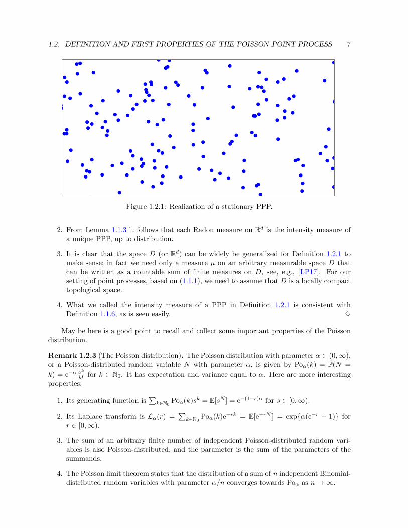
In Figure 1.2.1 we present a realization of a PPP. Let us further make a number of comments:

Remark 1.2.2. 1. We can certainly also drop the set D, i.e., put it equal to Rd, since thedependence on D can be absorbed in µ. Indeed, a measure µ on D can be trivially extendedto a measure on Rd with the value zero, and the PPPs that are induced by µ on D andthe one that is induced by its extension on Rd are equal to each other in distribution, afterrestricting to D.

1.2. DEFINITION AND FIRST PROPERTIES OF THE POISSON POINT PROCESS 7

Figure 1.2.1: Realization of a stationary PPP.

2. From Lemma 1.1.3 it follows that each Radon measure on Rd is the intensity measure ofa unique PPP, up to distribution.

3. It is clear that the space D (or Rd) can be widely be generalized for Definition 1.2.1 tomake sense; in fact we need only a measure µ on an arbitrary measurable space D thatcan be written as a countable sum of finite measures on D, see, e.g., [LP17]. For oursetting of point processes, based on (1.1.1), we need to assume that D is a locally compacttopological space.

4. What we called the intensity measure of a PPP in Definition 1.2.1 is consistent withDefinition 1.1.6, as is seen easily. 3

May be here is a good point to recall and collect some important properties of the Poissondistribution.

Remark 1.2.3 (The Poisson distribution). The Poisson distribution with parameter α ∈ (0,∞),or a Poisson-distributed random variable N with parameter α, is given by Poα(k) = P(N =

k) = e−α αk

k! for k ∈ N0. It has expectation and variance equal to α. Here are more interestingproperties:

1. Its generating function is∑

k∈N0Poα(k)sk = E[sN ] = e−(1−s)α for s ∈ [0,∞).

2. Its Laplace transform is Lα(r) =∑

k∈N0Poα(k)e−rk = E[e−rN ] = expα(e−r − 1) for

r ∈ [0,∞).

3. The sum of an arbitrary finite number of independent Poisson-distributed random vari-ables is also Poisson-distributed, and the parameter is the sum of the parameters of thesummands.

4. The Poisson limit theorem states that the distribution of a sum of n independent Binomial-distributed random variables with parameter α/n converges towards Poα as n→∞.


5. Given a Poisson-distributed random variable N with parameter α and independent andidentically distributed (i.i.d.) Bernoulli random variables Y1, . . . , YN with parameter p,then

∑Ni=1 Yi is Poisson-distributed with parameter pα.

6. If N is Poisson-distributed with parameter αt with α, t > 0, then P(N ≥ k) = P(E1 +· · · + Ek ≤ t) for any k ∈ N, where (Ei)i∈N is a sequence of i.i.d. variables having theexponential distribution with parameter α.

The superposition principle 5. is the main reason why the Poisson distribution is the ’right’distribution for the PPP, which can be seen by considering the distribution of the PPP non-disjoint sets. 3

Definition 1.2.1 is only in terms of the counting variables NX(A), but we would like to havethe object X also as an explicit S(D)-valued random variable. This is provided by the followingconstruction.

Lemma 1.2.4 (Construction of a PPP). Assume that µ is a measure on D with µ(D) ∈ (0,∞).Let N(D) be a Poisson random variable with parameter µ(D). Put I = 1, . . . , N(D). GivenN(D), let X = (Xi)i∈I be a collection of independent random points in D with distributionµ(·)/µ(D). Then the counting variables defined in (1.1.3) form a PPP with intensity measure µin the sense of Definition 1.2.1.

This construction works a priori only for finite intensity measures, but if µ is infinite, butσ-finite, then one can decompose D into countably many measurable sets with finite µ-measure,construct the point process on the partial sets according to Lemma 1.2.4 independently andput all these point processes together in order to obtain a PPP with intensity measure µ on D.It is an exercise to show that this construction works and that the resulting point process isindependent of the chosen decomposition of D; this is basically the proof of Lemma 1.2.8 below.

Remark 1.2.5 (Absolutely continuous intensity measures). If µ has a Lebesgue density, moregenerally if it has no atoms (sites x ∈ D with µ(x) > 0), then it is easy to see that the pointsof the corresponding PPP are almost surely located at mutually distinct sites, i.e., Xi 6= Xj forany i 6= j. Since we want to model the locations of human beings, we will assume this in mostof the following. 3

Example 1.2.6. 1. The standard PPP on D = Rd is obtained for the intensity measureλLeb, where λ ∈ (0,∞) is the intensity. Since Leb is shift-invariant, the correspondingpoint process is stationary (see Definition 1.1.7) and often referred to as a homogeneousPPP. Actually, since λLeb is the only shift-invariant measure on Rd, every shift-invariantPPP has this as its intensity measure for some λ ∈ (0,∞), see Lemma 1.1.8. Furthermore,its distribution is also isotropic, i.e., rotationally invariant.

2. For D = Zd and µ the counting measure on D, the corresponding PPP is a discrete variantof the standard PPP. It is obtained by realizing independent and identically distributedPoisson variables for each z ∈ Zd and putting that number of points into z. Alternatively,one can, for any finite set Λ ⊂ Zd, generate a Poisson random variableN(Λ) with parameter#Λ, and distribute N(Λ) points independently and uniformly over Λ, decompose Zd intosuch sets and add all these points independently in all of Zd; the resulting superpositionis the desired PPP.

1.2. DEFINITION AND FIRST PROPERTIES OF THE POISSON POINT PROCESS 9

3. If we want to model the locations of users in a given city D, then µ should reflect areaswith low density like lakes, forest and fields, where the Lebesgue density of µ should below, and high densities like highly frequented areas and places, where it should be high.

4. The one-dimensional standard PPP has enormous importance in the modeling of randomtimes, in particular in the theory of time-homogeneous Markov chains in continuous time.For d = 1, another interesting characterization of the PPP is possible: the distances ofneighboring pairs of points of the PPP are i.i.d. exponentially distributed random variableswith the same parameter as the PPP has; see also the last property that we mention inRemark 1.2.3. This is directly connected with the famous property of memorylessness ofthe process of times at which the points appear, see also Chapter 5. However, we will notelaborate on these nice properties here, since we are mainly interested in d ≥ 2. 3

Example 1.2.7 (Contact distance). The contact distance of a space point u ∈ D to a setx = xi : i ∈ I ∈ S(D) is defined by

dist(u, x) = inf‖u− xi‖ : i ∈ I. (1.2.2)

This is the radius of the largest ball around u that contains no point of x. If X is a PPP withintensity measure µ, then the distribution function of dist(u,X) is easy to find:

P(dist(u,X) < r) = P(Br(u) ∩ X 6= ∅) = 1− P(NX(Br(u)) = 0) = 1− e−µ(Br(u)), (1.2.3)

where Br(u) is the open ball around u with radius r. 3

Let us derive some important and simple properties of Poisson point processes. First, weidentify the distribution of the superposition of independent such processes.

Lemma 1.2.8 (Superposition of PPPs). Let µ1 and µ2 be two measures on D and let X(1) =(X(1)

i )i∈I1 and X(2) = (X(2)

i )i∈I2 be independent PPPs with intensity measures µ1 and µ2, respec-tively. Then, X(1)

i : i ∈ I1 ∪ X(2)

i : i ∈ I2 is a PPP with intensity measure µ1 + µ2.

The proof uses the well-known property of the sum of independent Poisson random variablesto be again Poisson, see Remark 1.2.3. An extension to superpositions of countably manyindependent PPPs is straightforward.

Another operation that goes well with PPPs is random thinning, i.e., the random removalof some of the points.

Lemma 1.2.9 (Random thinning of PPPs). Let X = (Xi)i∈I be a PPP in D with intensitymeasure µ. With a probability p ∈ [0, 1], given X, we keep independently any of the particles Xi.Then, the remains are a PPP with intensity measure pµ.

Also proving this is an elementary exercise, which is based on Property (5) in Remark 1.2.3.

Now we can easily realize many PPPs on one probability space with many different intensitymeasures:

Corollary 1.2.10 (Realization of superpositions). Let µ be a measure on D with µ(D) ∈ (0,∞),then we can, for any p ∈ [0, 1], construct the PPPs with intensity measure pµ on one probabilityspace as follows: Given a Poisson-distributed random variable N with parameter µ(D), wepick N i.i.d. random sites X1, . . . , XN in D with distribution µ/µ(D) and N i.i.d. randomvariables U1, . . . , UN that are uniformly distributed on [0, 1], independently of X1, . . . , XN . ThenXi : Ui ≤ p is a PPP with intensity measure pµ.


Here is another, quite general, way to construct a PPP out of another one: by a measurablemapping.

Theorem 1.2.11 (Mapping theorem). Let X = (Xi)i∈I be a PPP with intensity measure µ onD ⊂ Rd, and let f : D → Rs be a measurable map. Then, f(X) = (f(Xi))i∈I is a PPP in Rswith intensity measure µ f−1.

Let us note that, in the context of telecommunications, in order to avoid that the imagePPP has an intensity measure which is not atom-less, we must assume that µ(f−1(y)) = 0 forany y ∈ Rs.

In some situations, the following formulas may be useful. Their proofs are exercises.

Lemma 1.2.12. Let X be a PPP on D with intensity measure µ such that µ(D) ∈ (0,∞).Then, for any measurable function f : S(D)→ [0,∞),

E[f(X)] = e−µ(D)f(∅) + e−µ(D)∑n∈N

1

n!

∫Dn

f(x1, . . . , xn

)µ⊗n

(d(x1, . . . , xn)

).

Lemma 1.2.13. Let X be a PPP on D with intensity measure µ, and let A1 and A2 be twomeasurable subsets of D with µ(A1), µ(A2) <∞, then the covariance of NX(A1) and NX(A2) isequal to µ(A1 ∩A2).

1.3 The Campbell moment formulas

As always, we let D ⊂ Rd be a measurable (bounded or unbounded) subset of Rd, the com-munication area. In Section 1.1, we defined two topologies on S(D) by means of the mapsx 7→ Sf (x) =

∑i∈I f(xi) (see (1.1.2)) for certain functions f : D → R. Hence, the expectation

E[Sf (X)] will be an important tool for characterizing the distribution of a random point processX. We will give a formula for this.

Furthermore, the Laplace transform LX(f) (see (1.1.4)) turned out in Lemma 1.1.4 touniquely determine the distribution of a random point process X, hence it will also be use-ful to have explicit formulas for this. This functional has the great advantage that it alwaysyields a finite value for nonnegative functions f and has very nice properties with respect to con-vergence of the point process, as an application of the bounded convergence theorem is alwayspossible, see Section 1.7. We will also give a handy formula for this in the case of a PPP.

Theorem 1.3.1 (Campbell’s theorem). Let X be a point process on D with intensity measureµ, and let f : D → R be integrable with respect to µ, then

E[Sf (X)] =

∫Df(x)µ(dx). (1.3.1)

If X is even a PPP, then for nonnegative f ,

LX(f) = E[e−Sf (X)] = exp(∫

D(e−f(x) − 1)µ(dx)

). (1.3.2)

The proofs are easily done with the help of a measure-theoretic induction and the fact thatE[e−γY ] = exp

(λ(e−γ−1)

)for any Poisson-distributed random variable Y with parameter λ > 0

and any γ ∈ R.

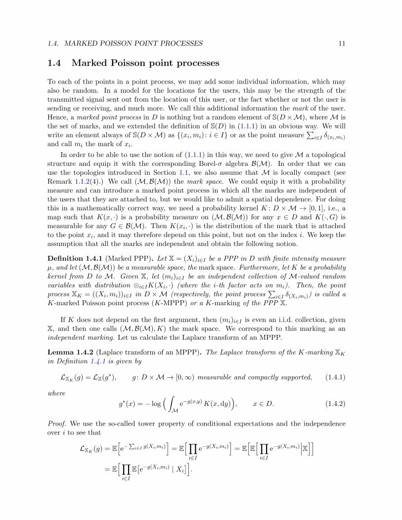
1.4. MARKED POISSON POINT PROCESSES 11

1.4 Marked Poisson point processes

To each of the points in a point process, we may add some individual information, which mayalso be random. In a model for the locations for the users, this may be the strength of thetransmitted signal sent out from the location of this user, or the fact whether or not the user issending or receiving, and much more. We call this additional information the mark of the user.Hence, a marked point process in D is nothing but a random element of S(D×M), whereM isthe set of marks, and we extended the definition of S(D) in (1.1.1) in an obvious way. We willwrite an element always of S(D×M) as (xi,mi) : i ∈ I or as the point measure

∑i∈I δ(xi,mi)

and call mi the mark of xi.

In order to be able to use the notion of (1.1.1) in this way, we need to giveM a topologicalstructure and equip it with the corresponding Borel-σ algebra B(M). In order that we canuse the topologies introduced in Section 1.1, we also assume that M is locally compact (seeRemark 1.1.2(4).) We call (M,B(M)) the mark space. We could equip it with a probabilitymeasure and can introduce a marked point process in which all the marks are independent ofthe users that they are attached to, but we would like to admit a spatial dependence. For doingthis in a mathematically correct way, we need a probability kernel K : D ×M → [0, 1], i.e., amap such that K(x, ·) is a probability measure on (M,B(M)) for any x ∈ D and K(·, G) ismeasurable for any G ∈ B(M). Then K(xi, ·) is the distribution of the mark that is attachedto the point xi, and it may therefore depend on this point, but not on the index i. We keep theassumption that all the marks are independent and obtain the following notion.

Definition 1.4.1 (Marked PPP). Let X = (Xi)i∈I be a PPP in D with finite intensity measureµ, and let (M,B(M)) be a measurable space, the mark space. Furthermore, let K be a probabilitykernel from D to M. Given X, let (mi)i∈I be an independent collection of M-valued randomvariables with distribution ⊗i∈IK(Xi, ·) (where the i-th factor acts on mi). Then, the pointprocess XK = ((Xi,mi))i∈I in D ×M (respectively, the point process

∑i∈I δ(Xi,mi)) is called a

K-marked Poisson point process (K-MPPP) or a K-marking of the PPP X.

If K does not depend on the first argument, then (mi)i∈I is even an i.i.d. collection, givenX, and then one calls (M,B(M),K) the mark space. We correspond to this marking as anindependent marking. Let us calculate the Laplace transform of an MPPP.

Lemma 1.4.2 (Laplace transform of an MPPP). The Laplace transform of the K-marking XKin Definition 1.4.1 is given by

LXK (g) = LX(g∗), g : D ×M→ [0,∞) measurable and compactly supported, (1.4.1)

where

g∗(x) = − log(∫M

e−g(x,y)K(x, dy)), x ∈ D. (1.4.2)

Proof. We use the so-called tower property of conditional expectations and the independenceover i to see that

LXK (g) = E[e−

∑i∈I g(Xi,mi)

]= E

[∏i∈I

e−g(Xi,mi)]

= E[E[∏i∈I

e−g(Xi,mi)∣∣∣X]]

= E[∏i∈I

E[e−g(Xi,mi) | Xi

]].


Observe that

E[e−g(Xi,mi)

∣∣Xi

]=

∫MK(Xi,dy) e−g(Xi,y) = e−g

∗(Xi).

Substituting this yields the assertion.

Now let us come back to the assumption that the mark space M is a locally compacttopological space, see the remarks at the beginning of this section. Then Lemma 1.4.2 easilyimplies that the K-MPPP XK is nothing but a usual PPP on D ×M with intensity measureµ⊗K 2, where we slightly extended Definition 1.2.1 in the spirit of Remark 1.2.2(3).

Theorem 1.4.3 (Marking theorem). Let the situation of Definition 1.4.1 be given, and assumethat (M,B(M)) is locally compact and is equipped with the Borel-σ-algebra. Then XK is indistribution equal to the PPP on D ×M with intensity measure µ⊗K.

Proof. From the last assertion in Remark 1.1.1, we know that the distribution of a point processin D×M is uniquely determined by its Laplace transform. Hence, we only have to show that theLaplace transform of a PPP with intensity measure µ⊗K is identical to the one of a K-MPPP.Apply (1.3.2) to Lemma 1.4.2 to see that

LX(g∗) = exp(∫

D(e−g

∗(x) − 1)µ(dx))

= exp(∫

D

(∫MK(x,dy) e−g(x,y) − 1

)µ(dx)

)= exp

(∫D

∫M

(e−g(x,y) − 1

)µ(dx)K(x,dy)

)= exp

(∫D×M

(e−g − 1)d(µ⊗K)).

Now consult (1.3.2) once more (for D×M instead of D) to see that this is the Laplace transformof a PPP with intensity measure µ⊗K.

Having seen this, it is also clear that, it is not necessary to normalize K, since one canconstruct a realization of such a PPP also by first taking X as a PPP with intensity measureK(M)µ and then pick the marks with distribution K/K(M). The reason is that, for anyc ∈ (0,∞), the measures cµ⊗K/c and µ⊗K coincide.

It is also clear that, for any K-marked PPP (Xi,mi) : i ∈ I with intensity measure µ andmark measure K, the projected process Xi : i ∈ I is a PPP with intensity measure µ.

Example 1.4.4. Since the d-dimensional Lebesgue measure is the d-fold product measure ofthe one-dimensional Lebesgue measure, one could think that the standard PPP in Rd can beseen as a marked PPP in Rd−1 with marks in R. However, since the Lebesgue measure on Ris not finite, this is not covered by Definition 1.4.1. If the last factor R is replaced by somebounded measurable set and the Lebesgue measure by the restriction, then this interpretationis correct. 3

2Note that the measure µ ⊗K is defined by µ ⊗K(B) =∫B(1) µ(dx)K(x,B(2)

x ), where B(1) = x ∈ D : ∃y ∈M : (x, y) ∈ B and B(2)

x = y ∈M : (x, y) ∈ B.

1.5. CONDITIONING: THE PALM VERSION 13

1.5 Conditioning: the Palm version

Let X be a stationary point process on Rd that is, the distribution of X equals the one of X + zfor any z ∈ Rd. We would like to imagine that we are standing in one of the points Xi ∈ X of theprocess and watch the other points from there. In other words, we are interested in the processX − Xi, seen from the perspective of Xi. To be sure, this point Xi should be a typical one,i.e., not a point that is sampled according to any specific criterion. Since we are in a stationarysetting, the randomly chosen point Xi can be assumed to be located at the origin. Hence, aswe will explain heuristically below, we would like to look at the conditional version of X given0 ∈ X. The definition of this object needs some care, since the event 0 ∈ X has probabilityzero for stationary processes. The mathematically sound setup for this is Palm theory. Let usstart by giving the associated existence and uniqueness result including the proof.

Theorem 1.5.1 (Refined Campbell theorem). Suppose that X is a stationary point process onS(Rd) with finite positive intensity λ. Then, there exists a unique probability measure P o onS(Rd) such that

λ−1E[∑i∈I

f(Xi,X−Xi)]

=

∫Eo[f(x, ·)] dx, f : Rd × S(Rd)→ [0,∞) measurable. (1.5.1)

The measure P o is called the Palm distribution of X.

Proof. We prove the statement for f = 1B×A for bounded measurable B ⊂ Rd, A ⊂ S(Rd). Thefull statement then follows by the usual monotone class arguments. We define

νA(B) = E[∑i∈I

1Xi ∈ B1X−Xi ∈ A].

Then, by stationarity,

νA(B + z) = E[∑i∈I

1Xi − z ∈ B1X−Xi ∈ A]

= E[∑i∈I

1Xi ∈ B1X−Xi ∈ A]

= νA(B),

and thus νA is also stationary. Further, since νA(B) ≤ E(NX(B)) = λ|B|, νA is also locally finiteand thus νA must be equivalent to λALeb with λA = νA([0, 1]d). Then, defining the probabilitymeasure P 0(A) = λA/λ, we have

E[∑i∈I

1Xi ∈ B1X−Xi ∈ A]

= λP 0(A)|B|.

Conversely, for B ⊂ Rd with 0 < |B| <∞, the equality (1.5.1) yields

P 0(A) = (λ|B|)−1E[∑i∈I

1Xi ∈ B1X−Xi ∈ A],

which shows uniqueness.


Remark 1.5.2. 1. It is convenient to introduce an S(Rd)-valued random variable X∗ withdistribution P o on the original probability space. For example, if f does not depend on x,we write

λ−1E[∑i∈I

f(X−Xi)]

= E[f(X∗)].

2. Let us provide some illustration and interpretation for the Palm distribution. The l.h.s. ofequation (1.5.1) can be interpreted as the probability of an event for X, seen from a ’typical’user Xi ∈ X, i.e., from a user that is picked uniformly at random. But what means’uniformly’ for an infinite point cloud? And what about the r.h.s. of (1.5.1)? To give somesubstance to the idea of picking a ‘typical’ point, we pick Xi uniformly at random fromthe stationary point process X with intensity measure λLeb for some λ ∈ (0,∞), in somecompact set A with positive Lebesgue measure, say a centered box. That is, we considerthe distribution of

∑i∈I δXi(A)δX−Xi, properly normalized. Note that the normalization

is 1/E[∑

i∈I δXi(A)] = 1/E[NX(A)] = 1/λLeb(A). The probability of an event Γ in S(Rd)is then equal to

1

λLeb(A)E[∑i∈I

δXi(A)1X−Xi ∈ Γ].

Actually, it turns out that this does not depend on A. Indeed, considering a partition(Dk)1≤k≤n of A consisting of connected Lebesgue-positive sets, we can rewrite this as

1

λLeb(A)

n∑k=1

E[∑i∈I

δXi(Dk)1X−Xi ∈ Γ∣∣∣NX(Dk) > 0

]P(NX(Dk) > 0).

Now, considering the limit of finer and finer partitions, we observe that P(NX(Dk) > 0) =λ|Dk|+o(λ|Dk|) and thus the above sum, in the spirit of a Riemann sum, should convergeto a limiting expression of the form

1

λLeb(A)λ

∫AE[1X− x ∈ Γ|x ∈ X

]dx. (1.5.2)

Now, by translation invariance, E[1X−x ∈ Γ|x ∈ X

]= P(X ∈ Γ|o ∈ X), where we write

o for the origin. We arrive at the heuristic equality

1

E[NX(A)]E[∑i∈I

δXi(A)1X−Xi ∈ Γ]

= P(X ∈ Γ|o ∈ X).

Note that the right-hand side is independent of A. The equality explains heuristicallythe relationship between the idea of a PPP seen from a typical point and the processconditioned on having a point at the origin. The distribution P(X ∈ ·|o ∈ X) = P 0(·) =P(X∗ ∈ ·) is then the Palm version of the distribution of X.

3. Following the same line of ideas, a closely related result can be formulated, called thereduced Campbell-Little-Mecke formula, which does not use stationarity. It states theexistence of the reduced Palm distribution P !

x for x ∈ Rd that is characterized by theequation

E[∑i∈I

f(Xi,X− δXi)]

=

∫E!x[f(x, ·)]µ(dx),

where µ is the intensity measure of X. Note that here the process is not shifted but rathera random point is removed, compare also to the expression (1.5.2). 3

1.6. RANDOM INTENSITY MEASURES: COX POINT PROCESSES 15

Theorem 1.5.1 is formulated for general stationary point processes. In the special case of ahomogeneous PPP, the Palm distribution has a particularly simple form, as can be understoodfrom the following argument. Since the event o ∈ X has measure zero under the PPP X, weinstead condition, for some ε > 0, on the event NX(Bε(0)) = 1 (which has positive probability)and perform the limit ε ↓ 0. Let us see what this gives for a counting variable NX(A) for somebounded open 0 ∈ A ⊂ Rd. Then,

P(NX(A) = n | NX(Bε(0)) = 1) =P(NX(A \Bε(0)) = n− 1, NX(Bε(0)) = 1)

P(NX(Bε(0)) = 1)

= P(NX(A \Bε(0)) = n− 1)

→ P(NX(A \ 0) = n− 1) = P(NX∪0(A) = n)

as ε ↓ 0. This suggests that the limiting conditioned process should be nothing but the processX ∪ 0. This is made precise in the following result. It states that Poisson processes are evencharacterized by this property.

Theorem 1.5.3 (Stationary Mecke-Slivnyak theorem). Let X be a stationary point process withintensity λ > 0. Then, X is a PPP if and only if

E[f(X∗)] = E[f(X ∪ 0)], f : S(Rd)→ [0,∞) measurable.

Remark 1.5.4. 1. The stationary Mecke-Slivnyak theorem is a special case of the more gen-eral Mecke-Slivnyak theorem, which does not use stationarity but some mild assumptionson the intensity measure µ. It states that a PPP X is characterized by the equation

E[∑i∈I

f(Xi,X)]

=

∫E[f(x,X ∪ x)

]µ(dx), f : Rd × S(Rd)→ [0,∞) (1.5.3)

In other words, for PPP, the reduced Palm distribution is equal to the original distribution.

2. The Mecke-Slivnyak theorem can also be seen as a generalization of Campbell’s theo-rem 1.3.1, which considers functions f(Xi,X) = f(Xi) not depending on X. 3

Example 1.5.5 (Contact distance distribution for homogeneous PPPs). Recall from Remark 1.2.7the contact distance dist(u, x) of a space point u ∈ D to a point set x = xi : i ∈ I ∈ S(D).If X is a homogeneous PPP with intensity λ, then P(dist(u,X) ≤ r) = P(dist(o,X∗) ≤ r) forall u ∈ D. In words, the distance of a typical point from a homogeneous PPP to its nearestneighbor in the PPP is distributed exactly as the distance from any fixed point. 3

1.6 Random intensity measures: Cox point processes

Modeling a system of telecommunication devices in space via a homogeneous PPP represents asituation where no information about the environment or any preferred behavior of the devicesis available. To some degree this can be compensated by the use of a non-homogeneous PPPwith intensity measure µ, where now areas can be equipped with higher or lower user density.Thereby we leave the mathematically nicer setting of spatial stationarity, but at least we keepthe spatial independence. Nevertheless, also the independence of devices is an assumption that isoften violated in the real world and user behavior is usually correlated. One way to incorporatedependencies into the distribution of devices in space is to use Cox point processes.


In simple words, a Cox point processes is a PPP with random intensity measure Λ. Thedirecting random measure Λ can be interpreted as a random environment and the resultingprocesses is thus constructed via a two-step stochastic procedure. More specifically, let D ⊂ Rdbe a measurable set, and we assume Λ to be a random element of the space of all σ-finite measuresM(D) on D equipped with the smallest sigma algebra such that all evaluation mappings µ 7→µ(B) fromM(D) to [0,∞] are measurable for all measurable B ⊂ D. We call such Λ a randommeasure on D.

Definition 1.6.1 (Cox point processes). Let Λ be a random measure on D, then the PPP Xwith random intensity measure Λ is called a Cox point process directed by Λ.

For a realization of Cox point process see Figure 1.6.1. Let us make some comments.

Remark 1.6.2 (Properties of Cox point processes). 1. The expected number of points in ameasurable volume A ⊂ D is given by the expected intensity of A, i.e.,

E[NX(A)] = E[E[NX(A)|Λ]] = E[Λ(A)].

2. The Laplace transform of a Cox point process is given by

LX(f) = E[e−Sf (X)] = E[

exp(∫

D(e−f(x) − 1) Λ(dx)

)], (1.6.1)

for all measurable f : D → [0,∞). 3

The theory of Cox point processes provides a broad setting for modeling interesting spatialtelecommunication systems.

Example 1.6.3 (Absolutely continuous random fields). A large class of random environmentsΛ is given by measures having a non-negative random field ` = `xx∈Rd as a Lebesgue density,i.e., Λ(dx) = `x dx. On Rd, one often assumes ` to be stationary. For example, this includesrandom measures modulated by a random closed set Ξ, see [CSKM13, Section 5.2.2]. Here,`x = λ11x ∈ Ξ + λ21x 6∈ Ξ with parameters λ1, λ2 ≥ 0. For instance, Ξ could be givenby the Boolean model

⋃j∈J Br(Yj) of a PPP (Yj)j∈J , see Chapter 2, interpreted as a random

configuration of hot spots. Another important example is a random measure induced by ashot-noise field3, see [CSKM13, Section 5.6]. Here, `x =

∑j∈J k(x− Yj) for some non-negative

integrable kernel k : Rd → [0,∞) with compact support and a PPP (Yj)j∈J . 3

Example 1.6.4 (Random street systems). Very interesting for a realistic modeling of an urbanarea is a random environment Λ that is defined as the restriction of the Lebesgue measure to arandom segment process S in Rd, we think of d = 2. That is, S is a point process in the spaceof line segments [CSKM13, Chapter 8], which we want to assume as stationary for simplicity.Observe that S is a union of one-dimensional subsets, in particular a nullset with respect to thetwo-dimensional Lebesgue measure. However, there is a natural measure ν1 on S that attachesa finite and positive value to each bounded non-trivial line segment (indeed, its length). Thismeasure is the one-dimensional Hausdorff measure ν1 on S. Then we put Λ(dx) = ν1(S∩dx) andobtain a random measure on R2 that is concentrated on S. Indeed, this random environment Λis singular with respect to the two-dimensional Lebesgue measure.

3The name shot noise = Schroteffekt comes from the choice of k as a Gaussian-shaped function, which ap-proaches the outcome of a lead shot.

1.6. RANDOM INTENSITY MEASURES: COX POINT PROCESSES 17

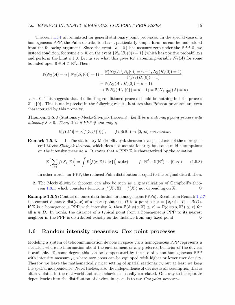
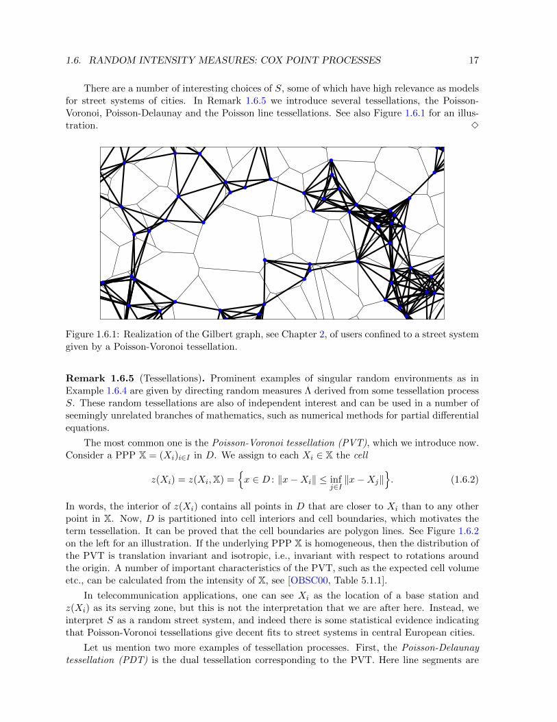
There are a number of interesting choices of S, some of which have high relevance as modelsfor street systems of cities. In Remark 1.6.5 we introduce several tessellations, the Poisson-Voronoi, Poisson-Delaunay and the Poisson line tessellations. See also Figure 1.6.1 for an illus-tration. 3

Figure 1.6.1: Realization of the Gilbert graph, see Chapter 2, of users confined to a street systemgiven by a Poisson-Voronoi tessellation.

Remark 1.6.5 (Tessellations). Prominent examples of singular random environments as inExample 1.6.4 are given by directing random measures Λ derived from some tessellation processS. These random tessellations are also of independent interest and can be used in a number ofseemingly unrelated branches of mathematics, such as numerical methods for partial differentialequations.

The most common one is the Poisson-Voronoi tessellation (PVT), which we introduce now.Consider a PPP X = (Xi)i∈I in D. We assign to each Xi ∈ X the cell

z(Xi) = z(Xi,X) =x ∈ D : ‖x−Xi‖ ≤ inf

j∈I‖x−Xj‖

. (1.6.2)

In words, the interior of z(Xi) contains all points in D that are closer to Xi than to any otherpoint in X. Now, D is partitioned into cell interiors and cell boundaries, which motivates theterm tessellation. It can be proved that the cell boundaries are polygon lines. See Figure 1.6.2on the left for an illustration. If the underlying PPP X is homogeneous, then the distribution ofthe PVT is translation invariant and isotropic, i.e., invariant with respect to rotations aroundthe origin. A number of important characteristics of the PVT, such as the expected cell volumeetc., can be calculated from the intensity of X, see [OBSC00, Table 5.1.1].

In telecommunication applications, one can see Xi as the location of a base station andz(Xi) as its serving zone, but this is not the interpretation that we are after here. Instead, weinterpret S as a random street system, and indeed there is some statistical evidence indicatingthat Poisson-Voronoi tessellations give decent fits to street systems in central European cities.

Let us mention two more examples of tessellation processes. First, the Poisson-Delaunaytessellation (PDT) is the dual tessellation corresponding to the PVT. Here line segments are


drawn such that any two cell centers Xi are connected by a line if and only if this line crossesexactly one cell boundary (or face in higher dimensions) in the PVT S. The PDT naturally hasvery similar locality properties as PVT, but completely different behavior for examples of itsvertex degree. More precisely, the typical Poisson-Voronoi cell has 6 line segments leading toa degree of 6 for the typical Poisson-Delaunay vertex. But, in the PVT, with probability one,only 3 line segments meet in a vertex. See Figure 1.6.2 on the right for an illustration.

Figure 1.6.2: Realizations of the PVT (left) and PDT (right).

Second, as another example of a tessellation process with relevance to telecommunications,let us mention Manhattan grids (MG), with the particular example of the rectangular Poissonline process (RPLT). The RPLT consists of perpendicular lines through the points of independentPoisson point processes representing landmarks along each axis in R2. Despite its popularityin stochastic geometry, this model has the serious drawback of only being able to representstreet systems where the distance between successive streets is exponentially distributed. Thisconstraint can be removed by replacing the Poisson renewal process by a stationary renewalprocess, that is, by a renewal process that is statistically invariant under shifts along the axis.See Figure 1.6.3 on the left for an illustration. The MG can be further refined by puttingadditional rectangular lines inside the boxes given by the MG. This construction gives risenested Manhattan grids (NMG), see Figure 1.6.3 on the right for an illustration. 3

Often, a key to the mathematical analysis of Cox point processes is their mixing properties:how strong and how far reaching are spatial stochastic dependencies? In the remainder of thissection we introduce the concept of stability as a tool to measures these dependencies. We denoteby ΛB the restriction of a measure Λ to a set B ⊂ Rd. Further, let Qr(x) = x + [−r/2, r/2]d

denote the cube with side length r > 0 centered at x ∈ Rd and put Qr = Qr(o). We definedist(ϕ,ψ) = inf|x− y| : x ∈ ϕ, y ∈ ψ for the distance between sets ϕ,ψ ⊂ Rd.

Definition 1.6.6 (Stabilizing random measures). A random measure Λ on Rd is called stabi-lizing, if there exists a random field of stabilization radii R = Rxx∈Rd, defined on the sameprobability space as Λ, such that

1. (Λ,R) is jointly stationary,

1.7. CONVERGENCE OF POINT PROCESSES 19

Figure 1.6.3: Realizations of the MG (left) and the NMG (right).

2. limr↑∞ P(supy∈Qr∩Qd Ry < r) = 1, and

3. for all r ≥ 1, the random variablesf(ΛQr(x))1 sup

y∈Qr(x)∩QdRy < r

x∈ϕ

are independent for all bounded measurable functions f : M(D) → [0,∞) and all finiteϕ ⊂ Rd with dist(x, ϕ \ x) > 3r for all x ∈ ϕ.

A strong form of stabilization is given if Λ is b-dependent in the sense that ΛA and ΛBare independent whenever dist(A,B) > b. The two models of Example 1.6.3 are b-dependentfor some b, and the random measure Λ concentrated on the Poisson-Voronoi tessellation S ofExample 1.6.4 is stabilizing.

Lemma 1.6.7 (The PVT is stabilizing). The stationary PVT on Rd is stabilizing.

Proof. The proof rests on the definition of the radius of stabilization as Rx = inf‖Xi−x‖ : Xi ∈X, for details see [CHJ17].

1.7 Convergence of point processes

Later, we want to discuss and analyze approximations of point processes, in order to arrive atmanageable formulas for complex situations. Hence, we need to discuss also convergence issuesfor point measures, which we do here. See also [DVJ03, Appendix A2] and [Re87]. The basiswas laid in Section 1.1, where two notions of distributions of point processes are discussed. Herewe proceed by one step and provide tools for characterizing convergence. One example that wefind important is the high-density limit, which we discuss at the end of this section. Here weencounter the situation that the point process converges towards some deterministic measure,i.e., not towards a point process. For this sake, we have to extend the set of random measuresfor which we consider convergence in distribution.


As before, we fix a measurable set D ⊂ Rd. The appropriate general setting of the followingis the setting where D is just some locally compact topological space, but, as in the precedingsections, we just keep this in mind and proceed with D ⊂ Rd. Instead of locally finite pointconfigurations (xi)i∈I ∈ S(D) or corresponding point measures

∑i∈I δxi , we will more generally

look at Radon measures on D, i.e., measures that assign to each compact subset of D a finitevalue. We want to characterize convergence of sequences of such measures in a natural way.We will do this for the two topologies that we introduced in Section 1.1, the vague and theτ -topology.

First, observe that the definition of vague and of τ -convergence of Radon measures on Ddirectly derives from a slight extension of Definition 1.1.1, i.e., it is defined by convergence ofall the test integrals against all the continuous, respectively the measurable, functions D → Rwith compact support. A variant of the Portmanteau theorem shows that this is the same asconvergence of the measures of compact subsets (whose boundary is a nullset with respect tothe limiting measure, for the vague case). This makes it easy to show, e.g., that on D = R, themeasure 1

n

∑i∈Z δi/n converges towards the Lebesgue measure.

Example 1.7.1. Vague and τ -convergence are local notions and say nothing about the totalmass, as one sees in the examples that δn on D = R converges to the zero measure and that themeasure on E = R with Lebesgue density 1l[−n,n] converges towards the Lebesgue measure asn→∞. 3

Remark 1.7.2 (Metrizability and measurability). There is a metric on the set of Radon mea-sures on D that induces the vague topology. Hence, the topological space of such measures isindeed a metric space. Its measurable structure is then given by the Borel σ-field. In particular,the maps µ 7→ µ(A) are measurable for any relative compact set A ⊂ D with boundary a nullset;actually these maps form a basis of this Borel σ-field; i.e., it is the smallest σ-field that makesthese maps measurable. 3

Remark 1.7.3 (Relative compactness of sets of measures). It can be deduced from Prohorov’stheorem that a sequence (µn)n∈N of Radon measures on D is relatively compact in the vaguetopology (i.e., that each subsequence contains a further subsequence that vaguely converges) ifand only if, for any relatively compact set A ⊂ D, the sequence (µn(A))n∈N is bounded. 3

Now we turn to sequences of random point measures, i.e., sequences of random variablestaking values in the set of point measures, and want to characterize possible limits. In principle,this has been settled by the preceding, since such measures are embedded in the set of Radonmeasures, and we established the topology of vague convergence on that set. Hence, it is, as atopological space, also a measurable space, and convergence of random variables taking values inthat space is to be understood in terms of weak convergence, sometimes also called convergencein distribution. To summarize this, we denote the set of Radon measures on D by R(D), then wecan recast the notion of the convergence of point processes, or more generally Radon measures,as follows.

Definition 1.7.4. A sequence (πn)n∈N of random Radon measures on D converges weakly (orconverges in distribution) towards a random Radon measure π on D if, for any continuousbounded function Φ: R(D)→ R, we have limn→∞ E(Φ(πn)) = E(Φ(π)).

Note that the continuity of Φ refers to any of two respective topologies that we consider onthe set of Radon measures, the vague and the τ -topology. In general, this characterization of

1.7. CONVERGENCE OF POINT PROCESSES 21

weak convergence is not very helpful, as it is a priori difficult to characterize all the continuousbounded functions on R(D). However, if all the measures π, π1, π2, . . . are point measures, thenthe situation is simpler:

Lemma 1.7.5 (Weak convergence of point measures in the vague- respectively τ -topology). Asequence (πn)n∈N of random point measures on D converges weakly (or in distribution) towardsa random point measure π if and only if the following holds. For any k ∈ N and for all relativecompact sets A1, . . . , Ak ⊂ E (additionally satisfying π(∂Ai) = 0 for the vague topology) almostsurely for all i ∈ 1, . . . , k, the vector (πn(A1), . . . , πn(Ak)) converges weakly towards the vector(π(A1), . . . , π(Ak)) as n→∞, i.e., if and only if, for any n1, . . . , nk ∈ N0,

limn→∞

P(πn(A1) = n1, . . . , π(Ak) = nk

)= P

(π(A1) = n1, . . . , π(Ak) = nk

).

We will also need convergence of Radon measures against (possibly deterministic) measuresthat are not point measures. For this, the possibly most handy criterion is the following. Wedenote the Laplace transform of a random measure π on D by

Lπ(f) = E[e−

∫D f(x)π(dx)

].

This notation is slightly misleading, since Lπ does not depend on π, but only on its distribution.

Lemma 1.7.6 (Convergence and Laplace transforms). A sequence (πn)n∈N of Radon measureson D converges weakly (or in distribution) towards some measure π on D if and only if theLaplace transforms converge, i.e., for any test function f : D → [0,∞) with compact support(continuous for the vague topology, just measurable for the τ -topology),

limn→∞

Lπn(f) = Lπ(f).

Later we will be interested in the high-density limit of a Poisson process in a compact subsetof Rd, in particular in the deviations away from the limit. Here we establish the limit itself.

Lemma 1.7.7 (Convergence of empirical measures). Let D ⊂ Rd be compact and µ a positiveand finite measure with Lebesgue density on D. For λ ∈ (0,∞), let X(λ) = (X(λ)

i )i∈Iλ be aPoisson point process in D with intensity measure λµ. Then, as λ → ∞, the random pointmeasure

Lλ =1

λ

∑i∈Iλ

δX

(λ)i

(1.7.1)

converges weakly (in both the vague and the τ -topology) towards µ as λ→∞.

Proof. According to Lemma 1.7.6, it is sufficient to check the convergence of the Laplace trans-form. Let f : D → [0,∞) be measurable, then, according to Campbell’s theorem,

LLλ(f) = LX(λ)(f/λ) = exp(∫

D(e−f(x)/λ − 1)λµ(dx)

). (1.7.2)

For any x, we see that the integrand with respect to µ(dx) converges towards −f(x). If fis integrable with respect to µ, then we can apply the dominated convergence theorem, since1 − e−y ≤ y for any y ∈ R, and therefore the integrand is bounded in absolute value by f(x).Hence, we see that the Laplace transform converges towards exp(−

∫D f(x)µ(dx)) = Lµ(f)


in this case. If f is not integrable with respect to µ, then we estimate LLλ(f) first againstLLλ(f ∧K) for some cutting parameter K, derive convergence towards exp−

∫f ∧K dµ and

use then the monotone monotone-convergence theorem for letting K → ∞ to see that LLλ(f)converges towards 0 = Lµ(f). In both cases, we have verified the convergence of the Laplacetransform for all nonnegative measurable test functions f .

Recall the interpretation that we rely on. The points Xi are the locations of the users(or other devices) of the telecommunication system in the communication area D. The inter-pretation of Lemma 1.7.7 is that the dense cloud of users in D approaches the density of theintensity measure µ, i.e., a multitude of microscopic information (every single user location) isapproximated by some much simpler macroscopic object, a density, for which there are goodperspectives for further analysis. One might argue that such a limiting setting is useless fordescribing human beings, since they cannot be squeezed infinitely strongly, but we are head-ing for approximate formulas, and many of the situations are in reality quite well described byapproximations via asymptotic formulas.

Chapter 2

Coverage and connectivity:the Boolean model

In this chapter, we discuss mathematical approaches to the two most fundamental questionsabout spatial telecommunication models:

• Coverage: How much of the area can be reached by the signals emitted from the users,respectably the base stations?

• Connectivity: How far can a message travel through the system in a multihop-functionality?

To do this, we introduce and study the most basic model for message transmission within aspatial system formed by a PPP X = Xi : i ∈ I of users or base stations, the Boolean model.In this model, which we introduce in Section 2.1, to each location Xi a random closed set Ξiis attached, the local communication zone that can be reached by a signal emitted from Xi.Then

⋃i∈I(Xi + Ξi) is the communication area, the set of locations that can be reached by any

message transmission. In Section 2.2, we study questions about the coverage of a given compactset C ⊂ Rd, i.e., about the probability that C can be reached by some signal. These are localquestions. In contrast, in Section 2.3, we consider global questions about whether or not thecommunication area possesses an unbounded connected component. This we will do only forhomogeneous PPPs and only for balls Ξi of a given fixed radius. In this simple but fundamentalsetting, we will distinguish two drastically different scenarios, the occurrence versus the absenceof percolation. The distinction is one important example of a phase transition and lies at theheart of a beautiful theory called continuum percolation. Both phases are non-trivial, as weformulate in Section 2.3. In order to carry out the proof for that in Section 2.5, we first needto rely on the discrete counterpart of the the theory, which we will prepare for in Section 2.4.Furthermore, we establish in Section 2.6 additional relevant connectivity questions related topercolation, and in Section 2.7 we discuss some peculiarities on percolation that arise for Coxpoint processes.

See [BB09a] and [BB09b] (which we follow in Sections 2.1 and 2.2) for application ofthe Boolean model to telecommunication, in particular coverage and percolation properties,and [BR06], [MR96] and [FM08] for mathematical proofs of continuum percolation properties.Standard references on the discrete part of the theory are [G89] and [BR06]. The Section 2.6about further interpretations of the percolation probability in telecommunications is largely self

23

24 CHAPTER 2. COVERAGE AND CONNECTIVITY: THE BOOLEAN MODEL

contained except for the shape theorem, see [YCG11]. The results about continuum percolationfor Cox point processes presented in Section 2.7 are less standard and taken from [CHJ17].

2.1 The Boolean model

Let X = Xi : i ∈ I be a point process in Rd with intensity measure µ. Again, we interpret theXi as the locations of the users or base stations of a spatial telecommunication system. Now,we extend the model by adding a random closed set Ξi ⊂ Rd around each user Xi and interpretXi + Ξi as the area that can be reached by a signal that is emitted from Xi. We call Ξi thelocal communication zone around Xi. The idea is that the strength of the signal decays quicklyin the distance, and a certain least strength is necessary for a successful transmission. Typicalchoices for Ξi are centered balls with random or deterministic radius, but more complex choicesare thinkable and have their right, e.g., when environmental conditions have to be taken care of.For example, if Xi is located on a street, then its local communication area Ξi will be shaped bythe houses left and right of the location Xi and will be approached by some rectangle, dependingon the location Xi. Apart from that, we will take the random sets Ξi, i ∈ I, as independent.Hence, we would like to see the Ξi as marks attached to the users Xi. Note that, under thisassumption, the case of Ξi being given by a Poisson-Voronoi cell, see (1.6.2), is not covered.

Definition 2.1.1 (Boolean model). Let X = Xi : i ∈ I be a PPP in Rd, and let K be aprobability kernel from Rd to the set of closed subsets of Rd. Consider the K-marking XK =∑

i∈I δ(Xi,Ξi) according to Definition 1.4.1). Then, the random set ΞBM =⋃i∈I(Xi + Ξi) is

called a Boolean model.

We have formally taken the set of all closed subsets of Rd as the mark space, and there isalso a natural σ-algebra on this set to turn this into a measurable space. However, this spaceis not a locally compact topological space, and therefore the above definition, strictly speaking,does not fall into Definition 1.4.1. However, there is no problem to concentrate the kernel ona much smaller set of closed sets, e.g., indexed by Rl for some set of parameters l in a naturalway that turns it into a locally compact topological space. One important example is the set ofcentered balls (or squares, or rectangles, ...) with a random radius. We will only think of suchexamples in these notes.

For simplicity, we will from now consider only independent K-markings, i.e., we will assumethat the random sets Ξi are i.i.d., not depending on the location Xi that they are attached to.That is, the kernel K is just one probability measure, which we will drop from the notation.The Boolean model ΞBM is interpreted as the total communication area, i.e., the (random) setthat is covered by the signals emitted from the set X.

2.2 Coverage properties

Let ΞBM be a Boolean model in the sense of Section 2.1, i.e., a PPP with an independent markingin a locally compact topological mark space. In this section we provide notions and methods todetermine probabilities of coverage, i.e., events that a given set or point lies in ΞBM. That is, welook only at one single transmission step from some Xi. Mathematically, this amounts to thestudy of the local structure of the random set ΞBM, i.e., a local question.

2.2. COVERAGE PROPERTIES 25

By Ξ we denote a generic random closed set that we use in our marking, i.e., a randomvariable having the distribution K. From now on, we will not use the kernel K anymore, butwill use P and E for probability and expectation with respect to Ξ. We will assume that itsdistribution satisfies

E[µ(C − Ξ)] <∞, for any compact C ⊂ Rd, (2.2.1)

where C − Ξ = x − y : x ∈ C, y ∈ Ξ. For example if C = 1 and Ξ = [−R,R] with someR ∈ (0,∞), then C−Ξ = [−R+1, 1+R] is the set of user locations x such that x+Ξ intersects C.Condition 2.2.1 ensures that the expected number of grains Ξ communicating with any compactC is finite. In particular, under this condition, also ΞBM is a random closed set itself.

The capacity functional of Ξ is defined as the function

TΞ(C) = P(Ξ ∩ C 6= ∅), C ⊂ Rd compact. (2.2.2)

This function can be seen as an equivalent of the distribution function of a real random variable;actually it determines the distribution of Ξ, according to Choquet’s theorem, see [M75].

Lemma 2.2.1. For any compact set C ⊂ Rd, the number

NXBM(C) = #i ∈ I : (Xi + Ξi) ∩ C 6= ∅

is a Poisson random variable with parameter E[µ(C − Ξ)].

Proof. Observe that the point process∑i∈I

δXi1l(Xi + Ξi) ∩ C 6= ∅

is an independent thinning of X (recall Lemma 1.2.9) with (space-dependent) thinning proba-bility

pC(x) = P((x+ Ξ) ∩ C 6= ∅) = P(x ∈ C − Ξ).

In the same way as in the proof of Lemma 1.2.9, one sees that this process is a PPP withintensity measure pC(x)µ(dx). Furthermore, NXBM

(C), the total number of its points, is aPoisson random variable with parameter equal to

∫Rd pC(x)µ(dx). With the help of Fubini’s

theorem, we identify this parameter as follows∫pC(x)µ(dx) =

∫P(x ∈ C − Ξ)µ(dx) = E

[ ∫1lx ∈ C − Ξµ(dx)

]= E[µ(C − Ξ)],

which ends the proof.

Lemma 2.2.2. The capacity functional is identified as

TΞ(C) = 1− e−E[µ(C−Ξ)], C ⊂ Rd compact.

Proof. Observe that TΞ(C) = P(NXBM(C) > 0) and use Lemma 2.2.1.


From now on we restrict to the stationary (or homogeneous) Boolean model, by which wemean that the intensity measure µ of the underlying PPP is equal to λLeb for some λ ∈ (0,∞),and we call λ the intensity of the Boolean model. It is clear that then also the capacity functionalof the Boolean model,

TΞBM(C) = P

(C ∩

⋃i∈I

(Xi + Ξi) 6= ∅)

(where the probability extends over the PPP X and the family of the Ξi’s) is shift-invariant, i.e.,TΞBM

(z +C) = TΞBM(C) for any z ∈ Rd and any compact set C ⊂ Rd. Also the volume fraction

p =E[Leb(ΞBM ∩B)]

Leb(B)(2.2.3)

does not depend on the compact set B ⊂ Rd, as long as it has positive Lebesgue measure. Thevolume fraction has the nice interpretation as the probability that the origin is covered by theBoolean model, as

p =1

Leb(B)

∫BE[1lx ∈ ΞBM] dx = E[1l0 ∈ ΞBM] = P(0 ∈ ΞBM) = TΞBM

(0).

In particular, Lemma 2.2.2 tells us that p = 1− e−E[Leb(Ξ)].

Remark 2.2.3 (Covariance of coverage variables). The volume fraction p is the expectation ofthe coverage variable at the origin, 1l0 ∈ ΞBM. The expectation of the product of the twocoverage variables 1l0 ∈ ΞBM and 1lz ∈ ΞBM can be calculated in an elementary way as

C(z) = E[1l0 ∈ ΞBM 1lz ∈ ΞBM

]= P(0 and z lie in ΞBM) = 2p−1+(1−p)2e−λE[Leb(Ξ∩(Ξ+z))].

The function C(z) is usually referred to as the covariance function of the Boolean model. It isthe probability that two points separated by the vector z are covered. The covariance of thetwo coverage variables is given by

C(z) = C(z)− p2 = −(1− p)2(1− e−λE[Leb(Ξ∩(Ξ+z))]).

3

The coverage probability of a given compact set C ⊂ Rd by a random closed set Ξ is definedas P(C ⊂ Ξ). In general, it is difficult to give explicit expressions for this quantity; however it isclear that it is not larger than TΞ(C), and we have equality for singletons C. In the literature,there are asymptotic results for the coverage probability for the homogeneous Boolean modelwith Ξ equal to a centered ball of radius rR, where R is a positive random variable and r is aparameter. These results are precise in the limit λ → ∞ of a highly dense PPP and r ↓ 0 ofvery small communication radii. We present one such result, see [J86, Lemma 7.3].

Theorem 2.2.4 (Asymptotic coverage probability). Assume that d = 2 and let C ⊂ R2 be acompact set whose boundary is a Lebesgue null set. Consider the Boolean model

ΞBM =⋃i∈I

(Xi +BrR(0)),

where the random radius R satisfies E[R2+ε] <∞ for some ε > 0. Put

φ(λ, r) = λr2πE[R2]− logLeb(C)

πr2E[R2]− 2 log log

Leb(C)

πr2E[R2]− log

E[R]2

E[R2].

2.3. LONG-RANGE CONNECTIVITY IN THE HOMOGENEOUS BOOLEAN MODEL 27

Then

P(C ⊂ ΞBM) = exp− e−φ(λ,r)

as λ→∞, r ↓ 0,

provided that φ(λ, r) tends to some limit in [−∞,∞].

One can use this result for finding, for a given compact set C, the number of Poisson points,depending on the size of the local communication balls that are needed for covering C with thecommunication area with a certain given positive probability. Indeed, for a given u ∈ R, coupleλ and r such that φ(λ(r), r)→ u with

λ(r) =1

λr2πE[R2]

(u+ log

Leb(C)

πr2E[R2]+ 2 log log

Leb(C)

πr2E[R2]+ log

E[R]2

E[R2]

).

Then, the coverage probability converges in the limit r ↓ 0

P(C ⊂ ΞBM)→ exp− e−u

.

2.3 Long-range connectivity in the homogeneous Boolean model

In this section, we consider the question of connectivity over long distances in the Boolean model,i.e, the question how far a message can travel through the system if it is allowed to make anunbounded number of hops. That is, we assume that a message can hop from user to userarbitrarily often, as long as it does not leave the communication area, and we ask how long thedistance is that it can travel. In other words, we consider a multi-hop functionality and use thesystem of users as a wireless ad hoc system, which carries the message trajectories without usageof base stations. We will consider this question only for a very special, but fundamental, versionof this model: the homogeneous Boolean model on the entire space Rd with deterministic localcommunication zones that are simply balls of a fixed radius. Hence, the Boolean model has onlyone effective parameter left, but it will turn out that it gives rise to a beautiful mathematicaltheory that is called continuum percolation. We will encounter an interesting phase transition inthis parameter: for large values, there is a possibility that the message can travel unboundedlyfar, and for small values its trajectory will always be bounded. Furthermore, we will be able toattack a number of further important quantities in later sections.

We assume that X = Xi : i ∈ I is a homogeneous PPP with intensity λ ∈ (0,∞), and therandom closed set Ξi that we put around each user location Xi is just a deterministic closedball BR/2(Xi) with a fixed radius R ∈ (0,∞). A message can now hop from Xi to Xj if andonly if ‖Xi − Xj‖ ≤ R, i.e., if and only if the straight line between them entirely lies in thecommunication area

⋃i∈I BR/2(Xi). This is the case if and only if the closed balls BR/2(Xi) and

BR/2(Xj) intersect. Therefore, we now have basically two mathematical models that expressconnectivity: either we conceive X as a random geometric graph (the so-called Gilbert graph)by drawing an edge between any two points Xi and Xj with distance ≤ R, or we consider theBoolean model

ΞBM =⋃i∈I

BR/2(Xi) (2.3.1)

and consider connectivity in the usual topological sense for subsets of Rd. We will proceed in thelatter model. Recall that the process is homogeneously distributed over Rd, and that we havejust two parameters, the intensity λ of X and the diameter R of the balls. We will write Pλ and


Figure 2.3.1: Realization of a homogeneous Boolean model.

Eλ for the probability and expectation in this model. In Figure 2.3.1 we present a realization ofsuch a Boolean model.

Let us denote by CR/2(x) the cluster (= connected component) of ΞBM that contains x.

Then CR/2(Xi) is the set of those space points in Rd that can be reached by a multi-hop trajec-tory starting at Xi through X. One of the most decisive properties of ΞBM is whether or notit has unboundedly large components. We say that ΞBM percolates or that percolation occursif the answer is yes. In this case, we also say that the points in the unbounded componentare connected to ∞. The notion of percolation is the base of everything that follows. It gavethe theory its name “continuum percolation”, since it is about the continuous space Rd. Inter-estingly, the first paper that introduced this model in 1961, see [G61], explicitly took wirelessmulti-hop communication as the prime example and motivation. There is a theory of discretepercolation (usually motivated by water leakage through porous stones), which we will encounterin Section 2.4 below.

Remark 2.3.1 (Percolation and message transmission). In the event that percolation occurs,there is at least one component C that is unboundedly large and contains infinitely many usersXi.As a consequence, messages that are emitted from such a user can reach, at least theoretically,infinitely many other users and can travel infinitely far. Note that this does not say anythingabout the reach of messages that are emitted from a bounded component, which certainly alsodo exist. In this event, the quality of transmission service is drastically better than in thecomplement event, such that we are highly interested in those values of the parameters thatmake this possible. 3

The most important quantity is the percolation probability

θ(λ,R/2) = Pλ(Leb(CR/2(o)) =∞). (2.3.2)

Since the PPP is locally finite, this is equal to the probability that CR/2(o) contains infinitelymany points of X.

2.4. INTERMEZZO: PHASE TRANSITION IN DISCRETE PERCOLATION 29

Remark 2.3.2 (Percolation probability via Palm calculus). Recall the Palm distribution P oλof X from Section 1.5. Then, by the stationary Mecke-Slivnyak theorem 1.5.3, the percolationprobability can be identified as

θ(λ,R) = P oλ(Leb(CR/2(o)) =∞).

By the interpretation of the Palm distribution, this quantity can be also interpreted as theprobability that the cluster CR(X) has infinite Lebesgue measure, for a randomly chosen userX ∈ X. The advantage of the Palm interpretation is that it can be easily extended to the settingof Cox point processes, see Section 2.7. 3

Because of the homogeneity of the PPP in space (more precisely, since the intensity measureis invariant under scaling), it is clear that the influence of the parameter R can easily be extractedas follows:

θ(λ,R) = θ(λRd), λ,R ∈ (0,∞), (2.3.3)

where we write θ(λ) = θ(λ, 1). Therefore, we will consider only θ(λ) in the following and willdrop R from the notation. It is clear from an application of Lemma 1.2.10 that θ is an increasingfunction. Hence, we can define the critical percolation threshold

λcr = infλ ∈ (0,∞) : θ(λ) > 0 = supλ ∈ (0,∞) : θ(λ) = 0 ∈ [0,∞], (2.3.4)

where we put sup ∅ = 0 and inf ∅ =∞. (From (2.3.3), we obtain that λcr(R) = λcrR−d if λcr(R)

denotes the critical percolation threshold for the Boolean model with interaction radius R.)

The start of the theory is the following.

Theorem 2.3.3 (The critical threshold is positive and finite). For any d ∈ N\1, λcr ∈ (0,∞).

The theorem says that, for some (sufficiently small) λ ∈ (0,∞), the percolation probabilityis zero, while for sufficiently large ones, it is positive, giving rise to non-trivial sub-and super-critical regimes. This is a clear manifestation of the occurrence of a phase transition. We givemore comments in Section 2.5 below. Before we prove Theorem 2.3.3 there, we must have a closerlook at the discrete version of percolation theory, as this will provide an inevitable mathematicalbase.

2.4 Intermezzo: phase transition in discrete percolation

As it is very often the case in the theory of point processes in continuous space, proofs rest on acomparison with the (much simpler) setting of a fixed geometry. Here, instead of a PPP on Rd,we will consider a Bernoulli field on the edges of Zd. That is, we put on every edge e betweenneighboring sites in Zd a Bernoulli random variable ξe ∈ 0, 1 with parameter p ∈ [0, 1], andassume that all these random variables are i.i.d.. Then (ξe)e is a Bernoulli field. The edge e iscalled open if ξe = 1 and closed otherwise. A realization of such a random field is said to exhibitpercolation if there exists an infinite connected component of open edges, where connectednessis defined in the usual sense on Zd. In this way, we are now working on the basic model of thetheory of discrete bond percolation, or just percolation. This likewise is a beautiful mathematicaltheory, which studies analogous questions, but is further developed than continuum percolation,due to the simpler setting of a fixed, discrete geometry. The standard reference for this theory


is [G89], but see also [BR06]. The main motivating application idea is a porous stone withhyper-cubic microstructure, one water source in the middle and walls between neighboring cellsthat are permeable to water with a certain probability, and then the question is whether or notthe surface of the stone is wet somewhere or not.

Note that we have now just one parameter p, the probability for openness. We denoteprobability and expectation in this model by Pp and Ep. In this model, we call two sites inZd connected if there is a sequence of open edges that form a nearest-neighbor path betweenthe two sites. We write C(x) for the cluster (= connected component) that contains x ∈ Zd.Similarly to 2.3.2 we introduce the percolation probability

θ(p) = Pp(#C(o) =∞) (2.4.1)

and the critical percolation threshold

pcr = infp ∈ [0, 1] : θ(p) > 0 ∈ [0, 1]. (2.4.2)

Here is the start of the theory of percolation, a result that will later be instrumental forproving the continuous version, Theorem 2.3.3:

Theorem 2.4.1 (Non-trivial critical threshold for Bernoulli bond percolation). For any d ∈N \ 1, we have that pcr ∈ (0, 1).

Proof. The proof naturally comes in two parts. First, we prove existence of a subcritical phase,i.e., that pcr > 0. For this, note that the event that the origin is connected to infinity is containedin the event that a self-avoiding path of open edges of a fixed length n ∈ N starts at the origin.Let Ψn denote the set of self-avoiding n-step paths starting at the origin, then, for any n ∈ N,we see that

θ(p) ≤ Pp(there exists η ∈ Ψn such that ξe = 1 for all e ∈ η)

≤∑η∈Ξn

Pp(ξe = 1 for all e ∈ η)

≤ |Ψn|pn ≤ (2dp)n.

But, if p < 1/(2d), then this quantity tends to zero as n tends to infinity and thus, θ(p) = 0.Therefore, pcr ≥ 1/(2d). (If one would estimate |Ψn| against 2d(2d−1)n−1, then even the boundpcr ≥ 1/(2d − 1) would follow, which proves absence of a supercritical regime in one spatialdimension.)

The proof for the existence of a supercritical phase, i.e., that pcr < 1, is more complicated.It suffices to prove that θ(p) > 0 for p ∈ (0, 1) close to 1. Note that if percolation occursin dimension d = 2, then it also occurs for higher dimensions since there it is even easier topercolate. (This is an idea that is difficult to make precise for continuum percolation.) In otherwords, the critical threshold for percolation is a decreasing function of the dimension and itsuffices to prove existence of a supercritical phase for dimension 2. This we will do now.

The strategy of the proof is an example of the famous Peierls’ argument, which leverages theprobabilistic costs of creating a blocking interface in the following sense. Consider the shiftedlattice Z2

∗ = Z2 + (1/2, 1/2) and call an edge e∗ in Z2∗ closed if the unique edge e in Z2 that

crosses e∗ is open and vice versa. Now, if the origin is not connected to infinity, there must exist

2.4. INTERMEZZO: PHASE TRANSITION IN DISCRETE PERCOLATION 31

a finite blocking interface of open edges in Z2∗ that surrounds the origin and contains one point

(n+ 1/2, 1/2) for some n ∈ N. Thus, we can bound

1− θ(p) ≤∑n∈N

Pp(there exists an open interface η∗ ⊂ Z2

∗

surrounding (0, 0) and passing (n+ 1/2, 1/2))

≤∑n∈N

Pp(there exists an open path in Z2

∗ of length 2n+ 4, passing (n+ 1/2, 1/2))

≤∑n∈N

(4(1− p))2n+4.

The factor 42n+4 is the number of paths of length 2n + 4. Now, for p close to one, this sum isstrictly smaller than 1 and thus, θ(p) > 1.

Let us mention some of many interesting and important results on discrete percolation.

Remark 2.4.2 (Survey on results on discrete percolation). 1. Numerical value. For Bernoullibond percolation on Z2, the critical threshold is proven to be pcr = 1/2 based on the self-duality of Z2. Except for a few examples (such as the triangular lattice to mention anotherone), there is no formula for pcr, and its numerical value can only be approached via sim-ulations.

2. Other criticality notions. Critical behavior of Bernoulli percolation can also be based onrelated, but different, quantities other than the percolation function, e.g., the value fromwhich on the expected size of the cluster containing the origin is infinite: p′cr = infp ∈[0, 1] : Ep(#(C(o))) =∞. For Bernoulli bond percolation on Z2, it is known that p′cr = pcr.

3. Number of infinite clusters. The random field Pp is invariant (in distribution) underlattice translations and is ergodic. This implies that, in the super-critical regime p > pcr,a percolation cluster appears almost surely (i.e, #(C(x)) =∞ for some x ∈ Zd), since thisevent is measurable with respect to the tail-sigma-algebra. Further, it can be shown thatthis infinite cluster is unique almost surely.

4. Sizes of finite clusters. A lot of work has been dedicated to further understand the clus-tering behavior in the two regimes. For example, in the subcritical regime, the probabilitythat the origin is connected to the complement of a centered box of side-length n is knownto be small exponentially fast in n. This is one ingredient of the proof of p′cr = pcr. Ina certain sense, the cardinality of any of the finite clusters (in both regimes) is known tobe a random variable with exponential tails, which implies that the largest of the finiteclusters in a box of radius n have about log n sites.

5. Less independence. Theorem 2.4.1 can be generalized with respect to the independence.E.g., if the probability p for a bond to be open is allowed to depend on neighboring bondsat distance ≤ k for some k ∈ N, then it can be shown that there exist two critical thresholdsp(1)cr ≤ p(2)cr such that below p(1)cr there is no infinite cluster almost surely and above p(2)cr thereis an infinite cluster almost surely.

6. Continuity of θ. Another big topic in the field is to determine the continuity properties ofp 7→ θ(p). It can be shown that it is continuous in [0, 1]\pcr and right-continuous at pcr.


Left-continuity at pcr so far could only be established for d = 2 and d ≥ 11. In particularfor 3 ≤ d ≤ 5 it is one of the big open questions for Bernoulli bond percolation.

7. Behavior of θ near criticality. It is widely believed that, on general graphs in place of Zd,the behavior of θ close to pcr is governed by a power law that depends only on some localfeatures of the underlying geometry. More precisely, in two dimensions it is expected thatθ(p) = (p− pcr)

β+o(1) as p ↓ pcr, with the critical exponent β = 5/36. This has been shownrigorously only for site percolation on the triangular lattice. 3

In Section 2.5 it will be important for us to note that discrete Bernoulli percolation on Zd orany other lattice can be also considered with openness attached to sites rather than bonds. Hereit is the sites in the lattice that are independently declared open with probability p ∈ [0, 1] (andclosed otherwise), and the notion of clusters (= connected components) is even more immediatethan in the bond setting. The resulting model is called Bernoulli site percolation. One canconvince oneself that it is harder to have site-percolation than to have bond-percolation, hencethe site-percolation threshold is not smaller than the bond-percolation threshold. Also for thesite-version of the model, versions of Theorem 2.4.1 have been proved for various lattices, see[G89] and [BR06]. In particular, we will rely in Section 2.5 on the non-triviality of the percolationthreshold for site percolation on the triangular lattice in two dimensions.

2.5 Proof of phase transition in continuum percolation

We are now going to apply the non-triviality of the percolation threshold for discrete percolationto the proof of the corresponding result in continuum, Theorem 2.3.3, which we are reallyafter. However, it will not be Theorem 2.4.1 that we directly apply, but its version for sitepercolation on the triangular grid in two dimensions, see [BR06], and correspondingly we willprove Theorem 2.3.3 only for d = 2.

The advantage of using the triangular lattice is that, in the dual face-percolation of hexagons,neighboring hexagons always share an edge and never only a vertex, like on Z2. Additionally,this comparison gives better bounds for the critical threshold. Indeed, site percolation on thetriangular lattice also has the critical threshold pcr = 1/2, see [BR06, Theorem 8, Chapter 5].The comparison is done via some appropriate discretization.

Proof of Theorem 2.3.3 for d = 2. Again, the proof naturally comes in two parts. For bothdirections we will use a partition (up to boundaries of Lebesgue null sets) of Rd into openhexagons Asx of side-length s > 0 centered at some points x ∈ R2. By default, we assumethat the origin is one of them. Note that the centers x form a triangular lattice Ts, where thebonds are drawn across the edges of neighboring hexagons. We call the center x of one of thesehexagons Asx open if it contains at least one Poisson point (i.e, at least one of the Xi’s) andclosed otherwise. Note that the probability for x to be open is given by

ps = 1− exp(−λLeb(Asx)), (2.5.1)

and note further that Leb(Asx) = 3√

3s2/2. It is clear from the homogeneity and the Poissoniannature of the PPP that openness of the sites in Ts defines a Bernoulli field of i.i.d. randomvariables. Hence, Ts is a Bernoulli site-percolation model as we briefly discussed at the end ofSection 2.4.

2.6. MORE ABOUT THE PERCOLATION PROBABILITY 33

Now, in order to show that λcr < ∞, note that any two points in neighboring hexagonshave distance at most

√13s. Recall that each ball around the Poisson points has diameter one.

Hence, if we pick s so small that√

13s < 1, then site-percolation on Ts implies percolation ofthe Boolean model XBM. Hence, if λ is sufficiently large such that ps = 1− exp(−λ3

√3s2/2) is

larger than the critical threshold 1/2 for site percolation on Ts, then we have percolation of theBoolean model. Explicitly, we have

λcr ≤ (26 log 2)/(3√

3).

Now we show that λcr > 0. Note that, if s > 1, percolation of the Boolean model impliessite-percolation on Ts. Hence, if λ is sufficiently small such that ps = 1 − exp(−λ3

√3s2/2) is

smaller than the threshold 1/2, then there is no percolation of the Boolean model. Calculatingagain, we arrive at

λcr ≥ (2 log 2)/(3√

3),

which completes the proof.

As for discrete percolation, we give now a list of further important results, most of whichare analogous, and the underlying proofs are often based on the discrete counterparts.

Remark 2.5.1 (More results on continuum percolation). 1. Numerical value. The numeri-cal value of the critical threshold is unknown in general. Rigorous bounds in d = 2 are0.174 < λcr < 0.843 [MR96, 3.9], the numerical value is λcr ≈ 0.6763475, derived bycomputer simulations [QZ07].

2. Uniqueness of infinite cluster. As in the discrete case, the Boolean model is invariantunder translations and ergodic in any dimension. Since percolation is a tail event, in thesuper-critical regime, a percolation cluster appears almost surely. Further, it can be shownthat the infinite cluster is also unique almost surely.

3. Size of bounded clusters. Again, as in the discrete case, in the subcritical regime, theprobability that the origin is connected to the complement of a centered box of side-lengthn, becomes small exponentially fast in n.

4. Complement of communication zone. It is equally interesting to study the vacant areaRd \ ΞBM. It can be shown that in the Boolean model there is at most one unboundedcomponent in the vacant area.

5. Random radii. The above proof can be extended to also cover the case of a Boolean modelwith centered balls of random radii > 0. The results here are the following. Let R bea random variable having the distribution of the radius of one of the balls. For d ≥ 2a supercritical regime exists, i.e., λcr < ∞. On the other hand, if E[R2d−1] < ∞, thenλcr > 0. For d = 1, if E[R] <∞, then λcr =∞, and if E[R] =∞, then λcr = 0. 3

2.6 More about the percolation probability

In this section we give some more information about the percolation probability θ. We returnto the setting where the radius of the balls around the Poisson points Xi is some arbitrary,fixed R ∈ (0,∞), and the intensity of the PPP X is λ. We write P and E for probability andexpectation.


Lemma 2.6.1 (Continuity of θ and exponential approach to 1 for large intensities). For anyR ∈ (0,∞), the map λ 7→ θ(λ,R) is continuous in [0,∞) \ λcr with asymptotics

limλ→∞

1

λlog(1− θ(λ,R)) = −Leb(BR(o)). (2.6.1)

The lower bound in equation (2.6.1) is easy to understand, since θ(λ,R) is lower boundedby the probability that the origin is isolated (i.e., that its R-ball has no Poison points), i.e.,1 − θ(λ,R) ≥ exp(−λLeb(BR(o))). For a full proof, see [P91, Corollary of Theorem 3]. Alsoconsider [FM08, Theorem 2.6.3] for a nice introduction in two dimensions. By the scale invari-ance, there is also an obvious corresponding result for R → ∞. In Figure 2.6.1 we present asketch of the graph of the percolation probability.

1

θ(λ)

λ

Figure 2.6.1: Approximative form of the percolation probability.

The fact that, in the super-critical regime, with probability one, there is only one infinitecomponent (see Remark 2.5.1) allows us to represent the probability of existence of a connectionbetween two far distant users via the percolation probability. More precisely, let

px = P(o! x) = P(there exists a path in X ∪ o, x connecting o and x) (2.6.2)

denote the probability that the origin is connected to a point x, then we have the followingresult.

Theorem 2.6.2 (Two-point connectivity). For any λ,R ∈ (0,∞), we have that lim‖x‖→∞ px =θ(λ,R)2.

We write from now on Qs(x) = [x− s2 , x+ s

2 ]d for the square around x ∈ Rd with side-lengths.

Proof. The main idea is that the only way that o and a distant site x can be connected is thateach of them belongs to the infinite cluster, two events that depend only on (sufficiently large)neighborhoods of o respectively x. The probabilities of these two events are roughly given bythe percolation probability each, and they become asymptotically independent if the distance islarge. Let us give some details.

For any y ∈ Rd, let Ey denote the event that there exists a path (i.e., polygon line connectingy and points of X) in ΞBM ∪BR(y), starting in y ∈ Rd and leaving the square Q‖x‖/3(y). Then

|px − θ(λ,R)2| ≤ |px − P(Eo ∩ Ex)|+ |P(Eo ∩ Ex)− θ(λ,R)2|. (2.6.3)

Note that Eo and Ex are independent and have the same probability. Hence, the second sum-mand can be bounded from above by

|P(Eo ∩ Ex)− θ(λ,R)2| ≤ 2|P(Eo)− θ(λ,R)| = 2(P(Eo)− θ(λ,R)).

2.6. MORE ABOUT THE PERCOLATION PROBABILITY 35

The right hand side is 2 times the probability of the origin being connected to Rd \Q‖x‖/3(o) butnot to infinity. This is not larger than 2 times the probability of the existence of an sufficientlythick interface of vacant space surrounding the origin at distance at least ‖x‖/3. In the super-critical regime, the probability for this event tends to zero (even exponentially fast) as ‖x‖ → ∞,see [MR96, Theorem 1].

The first summand on the right-hand side of (2.6.3), since the event that o! x is containedin the event Eo ∩ Ex, is equal to the probability that Eo ∩ Ex occurs but not o ! x.Note that this event is contained in the event that there exist two disjoint components in(ΞBM ∪ BR(o)) ∩ Q‖x‖(o) of diameter at least ‖x‖/6. But, the probability for this event alsotends to zero (even exponentially fast) as ‖x‖ → ∞, see [MR96, Lemma 4.1].

In the sub-critical regime, θ(λ,R) = 0 and px ≤ P(Eo), and P(Eo) tends to zero as ‖x‖ → ∞(even exponentially fast), see Remark 2.5.1 4..

A similar relation can be established between the percolation probability and the proportionof connected pairs of points in a growing volume. For this, let us denote by

πs = (sdλ)−2E[#(Xi, Xj) ∈ (X ∩Qs(o))2 : Xi ! Xj

](2.6.4)

the expected number of pairs of connected Poisson points in a square of side-length s, dividedby the expected number all Poisson point pairs. Then we have the following result.

Theorem 2.6.3 (Expected number of connected pairs). lims→∞ πs = θ(λ,R)2.

Proof. By the Mecke-Slivnyak theorem (1.5.3),

πs = (sdλ)−2E[∑i∈I

∑j∈I

1Xi ! Xj1Xi, Xj ∈ Qs(o)]

= s−2dλ−1

∫Qs(o)

E[∑j∈I

1x! Xj1Xj ∈ Qs(o)]

dx+ (sdλ)−1

= s−2d

∫Qs(o)

∫Qs(o)

P(x! y) dxdy + (sdλ)−1

= s−2d

∫Qs(o)

∫Qs(o)

P(o! (y − x)) dxdy + (sdλ)−1

= s−2d

∫Qs(o)

∫Qs(x)

P(o! z) dzdx+ (sdλ)−1.

Hence, |πs − θ(λ,R)2| ≤ s−2d∫Qs(o)

∫Qs(x) |P(o ! z) − θ(λ,R)2| dxdz + (sdλ)−1 and by The-

orem 2.6.2, there exists an r > 0 such that for z ∈ Rd \ Qr(o) = (Qr(o))c we have |P(o !

z)− θ(λ,R)2| < ε. But then we can estimate for sufficiently large s that

|πs − θ(λ,R)2| ≤ s−2d

∫Qs(o)

Leb(Qs(x) ∩Qr(o))dx+ εs−2d

∫Qs(o)

Leb(Qs(x) ∩ (Qr(o))c)dx+ ε

≤ s−dLeb(Qr(o)) + 2ε.

Since ε was arbitrary, this finishes the proof.


We have seen that connectivity characteristics of a network represented by the Booleanmodel can be expressed in terms of percolation probabilities. For many types of telecommuni-cation services it is essential not only to know of the existence of a connection, but to be ableto satisfy constraints on the number of hops. Let us finish this section by explaining how a hopconstraint can be captured via the stretch factor , a fundamental characteristic in continuumpercolation.

To begin with, we extend the definition of the connectivity of two points by imposing a

constraint on the number of hops. For k ∈ N, we write ok! x if o and x can be connected in

ΞBM ∪BR(o) ∪BR(x) in at most k hops, and we write

pk,x = P(ok! x).

To understand the asymptotic behavior of pk,x for large values of k and distant points x, werequire a crucial auxiliary result known as the shape theorem. Let C denote the unique infiniteconnected component in the super-critical phase of percolation in the Boolean model.

Theorem 2.6.4 (Shape theorem). For λ > λcr there exists a deterministic and finite stretchfactor ρ = ρ(λ,R) such that

lim‖Xi−Xj‖→∞Xi,Xj∈C

T (Xi, Xj)

‖Xi −Xj‖= ρ(λ,R),

where T (x, y) denotes the smallest number of hops from x to y.

In words, the shape theorem states that the minimum number of hops to connect points inthe unique infinite connected component grows linearly in the distance between the end points,and the proportionality factor depends only on the two parameters. Loosely speaking, the shapetheorem shows that, asymptotically for large distances, the metric induced by shortest pathsbetween points becomes simply a scalar multiple of the Euclidean metric.

The definition of T (x, y) generalizes to arbitrary points in Rd via T (x, y) = T (q(x), q(y))with the point q(x) ∈ X denoting the closest Poisson point to x that is contained in the infiniteconnected component. In particular, by sub-additivity, T (x, y) ≤ T (x, z) + T (z, y) for anyx, y, z ∈ Rd, so that ET (o, ne1) ≤ nET (o, e1). Hence, in expectation,

ρ(λ,R) ≤ ET (o, e1).

The proof of Theorem 2.6.4 rests on the famous Kingman’s sub-additive ergodic theorem,see [YCG11]. With this, we can extend the representation formula in Theorem 2.6.2 to thesetting of a bounded number of hops.

Theorem 2.6.5. Let λ > λcr and r > 0 be arbitrary, then

lim‖x‖→∞

pr‖x‖,x = θ(λ,R)21ρ(λ,R) ≤ r.

Sketch of proof. First, the factor θ2 appears for the same reason as in Theorem 2.6.2: (1) distantpoints fare only connected if both are in the unique infinite connected component, and (2) theevents of being in the infinite component are close to being independent if the considered pointsare far away from each other. By Theorem 2.6.4, the stretch factor converts constraints on thenumber of hops into a constraint on the Euclidean distance of the endpoints, thereby giving riseto the indicator on the right-hand side of the asserted limit.

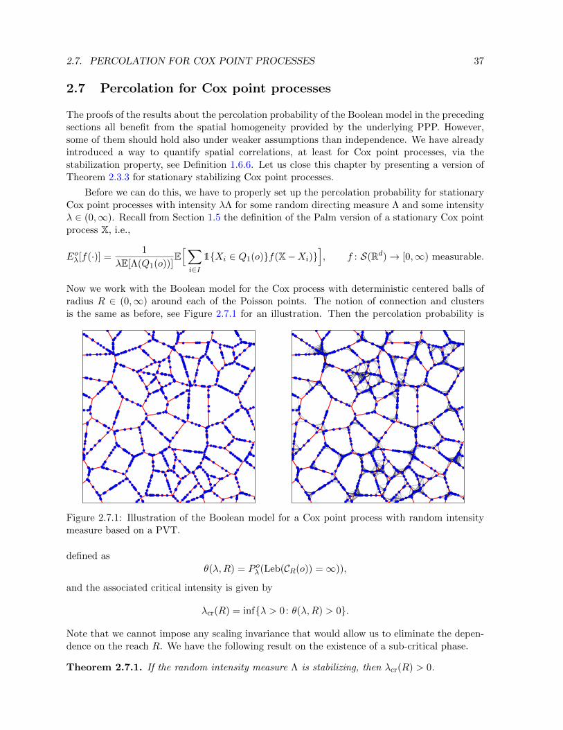
2.7. PERCOLATION FOR COX POINT PROCESSES 37

2.7 Percolation for Cox point processes

The proofs of the results about the percolation probability of the Boolean model in the precedingsections all benefit from the spatial homogeneity provided by the underlying PPP. However,some of them should hold also under weaker assumptions than independence. We have alreadyintroduced a way to quantify spatial correlations, at least for Cox point processes, via thestabilization property, see Definition 1.6.6. Let us close this chapter by presenting a version ofTheorem 2.3.3 for stationary stabilizing Cox point processes.

Before we can do this, we have to properly set up the percolation probability for stationaryCox point processes with intensity λΛ for some random directing measure Λ and some intensityλ ∈ (0,∞). Recall from Section 1.5 the definition of the Palm version of a stationary Cox pointprocess X, i.e.,

Eoλ[f(·)] =1

λE[Λ(Q1(o))]E[∑i∈I

1Xi ∈ Q1(o)f(X−Xi)], f : S(Rd)→ [0,∞) measurable.

Now we work with the Boolean model for the Cox process with deterministic centered balls ofradius R ∈ (0,∞) around each of the Poisson points. The notion of connection and clustersis the same as before, see Figure 2.7.1 for an illustration. Then the percolation probability is

Figure 2.7.1: Illustration of the Boolean model for a Cox point process with random intensitymeasure based on a PVT.

defined as

θ(λ,R) = P oλ(Leb(CR(o)) =∞)),

and the associated critical intensity is given by

λcr(R) = infλ > 0: θ(λ,R) > 0.

Note that we cannot impose any scaling invariance that would allow us to eliminate the depen-dence on the reach R. We have the following result on the existence of a sub-critical phase.

Theorem 2.7.1. If the random intensity measure Λ is stabilizing, then λcr(R) > 0.


The proof again rests on a comparison with Bernoulli percolation; we do not give details.This time, the comparison is first for a dependent discrete percolation system in the sense ofRemark 2.4.2 6.. In an additional step, the dependency can be stochastically bounded by anBernoulli site percolation with sufficiently low openness probability.

Note that, in order to establish existence of a supercritical regime, it is not sufficient toassume stabilization for the environment. Trivially, the environment may not put positiveweight on a connected region in space and consequently, even if λ is very large, the emergence ofa percolation cluster is impossible. This scenario can be avoided by putting another conditionon the environment which ensures enough connectivity. Recall the notation Qs = [−s/2, s/2]d.

Definition 2.7.2 (Connectedness of random measures). A stabilizing random measure Λ withstabilization radii Rx, x ∈ Rd, is called asymptotically essentially connected if for all n ≥ 1,whenever supy∈Q2n(o)

Ry < n/2, we have that

1. supp(ΛQn(o)) 6= ∅ and

2. supp(ΛQn(o)) is contained in a connected component of supp(ΛQ2n(o)).

The Poisson-Voronoi tessellation S of Example 1.6.4 does have this property.

Lemma 2.7.3 (The PVT is asymptotically essentially connected). The stationary PVT on Rdis asymptotically essentially connected.

Proof. The proof rests again on the definition of the radius of stabilization as Rx = inf‖Xi −x‖ : Xi ∈ X, for details see [CHJ17].

Now we can state our result about the existence of a super-critical phase for Cox pointprocesses.

Theorem 2.7.4. If the random intensity measure Λ is asymptotically essentially connected,then λcr(R) <∞.

Again the proof works via a discretization and comparison with a dependent Bernoullipercolation process, which can then be dominated by a super-critical independent Bernoullipercolation process.

Chapter 3

Interference:the signal-to-interference ratio

Let us proceed with our first steps in the application to a spatial random telecommunicationnetwork. Our basic model is a PPP X = Xi : i ∈ I in Rd, which is the set of locations ofthe users (or devices, or base stations, ...) of the system. We imagine that, at the time thatwe consider, from each of the locations a signal is emitted. Hence, there are possibly a numberof signals floating around the area. As a consequence, it may very well be that a given signalcannot be successfully transmitted, since it is suppressed by too much noise. This effect iscalled interference. In this section, we discuss one of the most widely used mathematical modelsfor describing interference, and show how to handle some of the most relevant properties. InSection 3.1, we introduce the basic tools for describing the signal strengths mathematically,and in Section 3.2, we introduce and discuss a criterion for successful transmission in terms ofthe signal-to-interference ratio. In Section 3.3 we present some results about the percolationproperties of the variant of the Boolean model where edges are drawn based on the signal-to-interference ratio.

3.1 Describing interference

The signals are propagated instantly and isotropically (i.e., radially symmetrically) into all spacedirections from the point of origin. However, there are fading effects by acoustic obstacles likethe medium or by more concrete ones like trees, fences, houses and so on, which make the signalstrength smaller and smaller as the distance to the transmission site increases. This fading istypically expressed in two ways. First, in terms of a (random) mark at the transmission site,accounting for the smaller non distant-based obstruction of the signal. Secondly, the fadingof the signals because of distance, is expressed in terms of a function ` : (0,∞) → [0,∞), thepath-loss function, i.e., `(r) is the strength of the signal in a distance r from the transmitter.This function should be decreasing with limr→∞ `(r) = 0 and limr↓0 `(r) = 1, since the receivedstrength cannot be larger than the emitted strength. Let us assume, that the transmission powerof each signal is identical, say one.

Very important is the kind of decay of `(r) for large r. The general ansatz is that it shoulddecay like a power of r, say `(r) ≈ r−α as r →∞, for some α > 0. The parameter α models theaverage path-loss in the medium that we consider: the more acoustic obstacles are there (e.g.,

39

40 CHAPTER 3. INTERFERENCE: THE SIGNAL-TO-INTERFERENCE RATIO

in areas with a high density of houses or walls), the larger α should be picked. Often, one justdetermines that α > d to ensure integrability, see below. Therefore, typical choices of ` are

`(r) = r−α or `(r) = (1 + r)−α or `(r) = min1, r−α. (3.1.1)

Note that the first choice, `(r) = r−α, is for our application not senseful, since it explodesfor small distances, but on the other side it has nice mathematical properties, for example aperfect-scaling property, such that many quantities of interest can explicitly be calculated.

Let us assume that at some site y ∈ Rd one receiver is located. The total amount of signalsthat (s)he receives is equal to

IX(y) =∑i∈I

`(‖Xi − y‖), y ∈ Rd, (3.1.2)

which is called the interference at y. Note that the interference at the origin, IX = IX(o), isequal to S`‖·‖(X) =

∑i∈I `(‖Xi‖), as defined in (1.1.2). Let us have a look at its expectation.

Example 3.1.1 (Mean interference at the origin). How large is the expected sum of the signalsthat one receiver at the origin experiences? Campbell’s formula from Theorem 1.3.1 gives

E[IX] = E[S`‖·‖(X)] =

∫Rd`(‖y‖)µ(dy),

where µ is the intensity measure of the point process X. Let us study the important special caseof a standard PPP X with intensity λ, and let us pick one of the two bounded choices of ` in(3.1.1). (Indeed, one can easily see that the perfect-scaling choice `(r) = r−α leads to an integralthat diverges for any value of α – either at ∞ or at zero). Hence, the finiteness of the integralexclusively hinges at the integrability of the integral of `(‖ · ‖) at infinity. The asymptotics fory →∞ are ∼ ‖y‖−α, hence we see that

E[IX] <∞ ⇐⇒ α > d.

This belongs to the reasons that often we will pick α > d or make the assumption that y 7→ `(‖y‖)is integrable with respect to µ: the interference is an integrable random variable. For both abovechoices of ` it is possible without difficulties to calculate the expectation of the interference.Campbell’s formula helps us also to find its variance explicitly, but for its finiteness we evenneed to assume that α > 2d. 3

Example 3.1.2 (The distribution of the interference). Let us describe a standard procedurefor describing the distribution of the interference at zero, IX, for a PPP X with general intensitymeasure µ and general path-loss function `. The two basic ingredients of this procedure are (1) anapproximation with the interference coming from a large ball, and (2) decomposition accordingto the number of users in that ball. However, we will see that an explicit identification of thedistribution is possible only in very particular cases.

Let IX[B] =∑

i∈I : Xi∈B `(‖Xi‖) denote the interference at zero coming from all users in aset B, and recall that NX(B), the number of users in B, is Poisson-distributed with parameterµ(B). Furthermore, recall from Lemma 1.2.4 that, given the event NX(B) = k, the k users inB are independent and identically distributed sites with distribution µ(dx)/µ(B), restricted to

3.1. DESCRIBING INTERFERENCE 41

B. We denote by Ba the centered ball around the origin with radius a. Let us try to calculatethe distribution function of IX. For any t ∈ [0,∞), we have

P(IX ≤ t) = lima→∞

P(IX[Ba] ≤ t) = lima→∞

∑k∈N0

e−µ(Ba)µ(Ba)k

k!P(IX[Ba] ≤ t | NX(Ba) = k)

= lima→∞

e−µ(Ba)∑k∈N0

µ(Ba)k

k!Pa( k∑j=1

Lj ≤ t),

(3.1.3)

where L1, . . . , Lk are k i.i.d. (0,∞)-valued random variables with the distribution of `(‖Y ‖). IfY ∈ Ba is distributed according to µ(dx)/µ(Ba) that is,

Pa(L1 ≤ t) =1

µ(Ba)

∫Ba

1l`(‖y‖) ≤ tµ(dy), t ∈ (0,∞).

It is not straight-forward to evaluate the right-hand side of (3.1.3), but such problems areubiquitous. The last term is the distribution function of a sum of k i.i.d. random variables andhence it looks promising to proceed instead with either the Fourier transform (characteristicfunction) or with the Laplace transform, since in both cases the probability term is decomposedin a product of k identical things, i.e., in a k-th power. In both cases, the k-sum can thereforebe evaluated with the help of the exponential series. Let us demonstrate this for the Laplacetransform: for any s > 0, we have

E[e−sIX ] = lima→∞

e−µ(Ba)∑k∈N0

µ(Ba)k

k!Ea[e−s

∑kj=1 Lj ]

= lima→∞

e−µ(Ba)∑k∈N0

µ(Ba)k

k!Ea[e−sL1 ]k

= lima→∞

e−µ(Ba) expµ(Ba)Ea[e−sL1 ]

= lim

a→∞exp

∫Ba

e−s`(‖y‖) µ(dy)− µ(Ba)

= exp∫

Rd

[e−s`(‖y‖) − 1

]µ(dy)

.

(This calculation is an alternate proof of Campbell’s theorem 1.3.1 for Laplace transforms.)

A similar calculation applies to Fourier transforms. Indeed, for any ω ∈ R, we see that

FIX(ω) = E[eiωIX ] = exp∫

Rd

[eiω`(‖y‖) − 1

]µ(dy)

.

Now, in order to identify the distribution of IX, one has to find formulas for the inversion of therespective transforms.

An explicit evaluation of this integral seems possible only for very particular choices, forexample µ the Lebesgue measure and `(r) = r−α. It is not clear how much one can learn formsuch model calculations, as the interference drastically depends on the choice of the path-lossfunction and on the users that are located close to the origin, and they may produce effects thatare typically unwanted and unrealistic. 3


Example 3.1.3 (Interference with individual transmission powers). Let us consider the casewhere each user Xi emits a signal with an individual transmission strength Pi ∈ (0,∞). Weassume that, given I, the PPP X = Xi : i ∈ I and the collection P = (Pi)i∈I of strengthsare independent, and that (Pi)i∈I is an i.i.d. collection. Then (Xi, Pi) : i ∈ I is a markedPPP. The interference at zero is now the random variable I(X,P ) =

∑i∈I Pi`(‖Xi‖). Its Laplace

transform is calculated as

E[e−sI(X,P ) ] = exp∫

Rd

∫(0,∞)

[e−sp`(‖y‖) − 1

]K(dp)µ(dy)

,

where K is the distribution of a transmission strength. In the special case µ = λLeb and`(r) = r−α, one can calculate in an elementary way that

E[e−sI(X,P ) ] = expλcd

∫(0,∞)

(ps)α/dK(dp)Γ(1− αd )

where Γ denotes the distribution function of the Gamma distribution. 3

3.2 The signal-to-interference ratio

The interference IX(y) at a given site y from transmissions from all the users Xi ∈ X is a measureof the total amount of noise that is received from all the messages that are present. Actually, thereceiver at y is interested to successfully understand a signal that comes from a particular userXi. The interference makes it hard that (s)he is successful. A precise mathematical criterionfor this success is given in terms of the signal-to-noise-and-interference ratio (SINR),

SINR(Xi, y,X) =Pi`(‖Xi − y‖)

N +∑

j∈I\i Pj`(‖Xj − y‖), y ∈ R. (3.2.1)

where N ∈ (0,∞) is the general noise in the system, Pi ∈ (0,∞) is the signal power of the i-thuser, and ` is a path-loss function as in Section 3.1. In words, SINR(Xi, y,X) is the quotientof the (wanted) signal strength that is received at y from the user Xi and the (unwanted) totalsum of the basic noise and all the other signal strengths transmitted from all the other users.If y = Xk for some Xk ∈ X, then in the interference term also the signal from Xj to Xk isneglected, i.e., we consider

∑j∈I\i,k Pj`(‖Xj −Xk‖).

If we want to neglect the general noise, then we put N = 0 and call the quantity in (3.2.1)the signal-to-interference ratio (SIR) and write it as SIR(Xi, y,X). Certainly, we can furthersimplify by putting Pi = 1 for any i. Both the noise N and the signal strengths Pi can be takenrandom.

The criterion is then formulated as:

The person at y can detect the signal from Xi ⇐⇒ SINR(Xi, y,X) ≥ τ, (3.2.2)

where τ ∈ (0,∞) is a technical constant, which measures the fineness of the ability to filter thewanted signal from the unwanted ones. The area of sites that can detect the signal emitted froma given Poisson site Xi ∈ X,

CXi = y ∈ Rd : SINR(Xi, y,X) ≥ τ (3.2.3)

3.2. THE SIGNAL-TO-INTERFERENCE RATIO 43

is called its SINR cell. The union of these cells,

ΞSINR =⋃i∈ICXi , (3.2.4)

is called the SINR model similar to the Boolean model in (2.3.1). We define the SINR coverageprobability

po(y) = P o(y ∈ Co) = TΞSINR(y), y ∈ Rd, (3.2.5)

as the probability (under the Palm measure) that a given site can be reached by a signal emittedfrom the origin; recall the capacity functional introduced in (2.2.2).

Remark 3.2.1 (Calculating the coverage probability). Note that this probability can be eval-uated using that

po(y) = P(Po`(‖y‖) ≥ τ

(N +

∑j∈I

Pj`(‖Xj − y‖)).

The probability involves the PPP X, the random noise N and the i.i.d. signal strength variablesPi; we assume that all these quantities are independent. It is difficult to obtain more explicitformulas in general; [BB09a] derives formulas involving Fourier transforms of the interferenceand of the signal strength variables. Here is an approach for the case that the signal strengthsPi are exponentially distributed with parameter c. This puts us in the lucky situation that wecan employ the Laplace transforms of N and of the interference I(X,P )(y) =

∑j∈I Pj`(‖Xj − y‖)

as follows.

po(y) =

∫ ∞0

P(P ≥ τs/`(‖y‖))P(N + I(X,P )(y) ∈ ds)

=

∫ ∞0

exp−cτs/`(‖y‖)P(N + I(X,P )(y) ∈ ds)

= LN+I(X,P )(y)(cτ/`(‖y‖))

= LN (cτ/`(‖y‖))LI(X,P )(y)(cτ/`(‖y‖)),

where we used that the Laplace transform of a sum of two independent random variables is equalto the product of the two Laplace transforms. For calculating the transform of I(X,P )(y), onemight use Example 3.1.3. In the simple case where N = 0 and `(r) = r−α for some α ∈ (0,∞),one can derive explicit results. 3

Remark 3.2.2 (Avoiding interference). In our interpretation, the sum over i in the sum inthe denominator of the SIR in 3.2.1 actually extends over the set of those users who transmitprecisely at the time that we consider. In a more complex model that takes a time developmentinto consideration, certainly this set can vary from time to time. Even more, if many users desireto transmit messages, then it will be absolutely necessary to distribute the times of transmissionsin such a way that, at each of the time instances, only a carefully chosen part of the messages issent out, such that the sum in the denominator is not too large. A strategy that guarantees thiswill possibly allow only a certain density of user to transmit at a given time instance. Further,since we are looking at a multi-hop system, each message will need to be assigned several suchhopping times, until it finally arrives at the intended receiver.

Finding or describing algorithms to achieve this belong to the theory of discrete optimization,but finding the abstract possibility to do this and proving bounds for the number of messagetransmissions per time unit is an exciting application of percolation theory. 3


3.3 SINR percolation

Given the point cloud X, the SINR gives us a more refined and more realistic rule to build arandom graph with vertices given by X. The classical Boolean model, where an edge is drawnbetween two points based on their mutual distance, can now be replaced by the SINR model,where a directed edge is drawn from Xi to Xj in X if SINR(Xi, Xj ,X) ≥ τ . In many systems,one considers a message transmission Xi → Xj successful only if also a confirmation messageXj → Xi is successfully transmitted. Hence, it makes good sense to introduce symmetry inthe bonds and consider the undirected graph having an edge between Xi and Xj in X if bothSINR(Xi, Xj ,X) ≥ τ and SINR(Xj , Xi,X) ≥ τ .

Let us introduce an additional parameter γ > 0, which allows us to tune the interferenceand write

SINRγ(Xi, y,X) =Pi`(‖Xi − y‖)

N + γ∑

j∈I\i Pj`(‖Xj − y‖), y ∈ R. (3.3.1)

We call the corresponding graph the SINRγ model.

Remark 3.3.1 (Relative versus total interference). The exclusion of the transmitter Xi in theinterference term in the denominator in (3.3.1) is a standard model assumption. However, undera suitable change of the connectivity parameter τ , the reduced interference

∑j∈I\i Pj`(‖Xj −

y‖) can be replaced by the total interference I(X,P )(y). Indeed, the condition SINRγ(Xi, y,X) ≥ τis equivalent to

Pi`(‖Xi − y‖) ≥ τ(N + γ

∑j∈I\i

Pj`(‖Xj − y‖))

= τ(N + γI(X,P )(y)− γPi`(‖Xi − y‖)

),

which is equivalent to Pi`(‖Xi − y‖) ≥ τ1+τγ (N + γI(X,P )(y)). 3

In contrast with the Boolean model, the SINRγ model has far-reaching correlations, and onemight think that its mathematical treatment should be much more difficult than the one of theBoolean model. This is in general true, but with respect to the degrees of its nodes, the SINRγ

model has surprisingly a rather simple property. Indeed, while the vertices in the Boolean modelin an infinite space have unbounded degrees (in the sense that, with probability one, there existsan infinite sequence of users (Xin)n∈N such that each Xin has at least n neighbors), in the SINRγ

model this cannot happen.

Lemma 3.3.2 (The SINRγ model has bounded degree). Let γ > 0, then in the SINRγ model,with probability one, each node has at most 1 + 1/(γτ) neighbors.

Proof. Let X0 be any user in X and denote by N0 the number of its neighbors. If N0 ≤ 1, thereis nothing to show. If N0 > 1, then with probability one, there exists a neighbor of X0 withsmallest signal power, i.e., there exists X1 ∈ X be such that for all i = 2, . . . , N0

P1`(‖X1 −X0‖) ≤ P1`(‖Xi −X0‖).

Then,

P1`(‖X1 −X0‖) ≥ τN + τγ∑

j∈I\0,1

Pj`(‖Xj −X0‖)

≥ τγ(N0 − 1)P1`(‖X1 −X0‖)and thus N0 ≤ 1 + 1/(γτ).

3.3. SINR PERCOLATION 45

In particular, if γ > 1/τ , then each node has at most one neighbor and the SINRγ modelhas components of size at most two.

Remark 3.3.3 (SINRγ model versus Boolean model). 1. For γ = 0, the interference is ne-glected and the SINRγ model becomes a Boolean model, where two users are connectedindependently from all the other users. Assuming that all users transmit at some fixedmaximum power P ∈ (0,∞), the (random) radius of interaction is then given by

R = supr ≥ 0: `(r) ≥ τN/P.

More specifically, for `(r) = r−α we have that R = (P/(τN))1/α. Recalling the statement5. in Remark 2.5.1, under some assumptions on the distribution of N , there exists anon-trivial λ∗cr ∈ (0,∞) marking the phase-transition point which separates a sub- andsupercritical regime of percolation.

2. Note that for any γ > 0, realization-wise, the SINRγ model is contained in the SINR0

model since interference can only decrease the connectivity. Hence, for λ < λ∗cr, the SINRγ

model is subcritical.

3. For λ > λ∗cr we know that

(a) the SINR0 model is supercritical and

(b) for γ > 1/τ , by Lemma 3.3.2, the SINRγ model is subcritical.

Hence, there must exist a critical 0 ≤ γcr(λ) ≤ 1/τ at which the SINRγ model has a phasetransition of percolation. 3

The following theorem makes statements about γcr(λ) under rather strong model assump-tions. A proof can be found in [DBT05].

Theorem 3.3.4. Let d = 2 and assume Pi = P and N to be fixed positive and finite numbers.Further assume that there exist 0 < δ < β and M > τN/P such that the pathloss functionsatisfies `(r) = 0 for all r > β and τN/P < `(r) < M for all r < δ. Then, there exists λ′ <∞and a function γcr : [λ′,∞) → (0,∞) such that, for λ > λ′ and γ < γcr(λ) there exists almostsurely an infinite component in the SINRγ model.

A more complete statement for the existence of a super-critical phase in the presence ofinterference is given in [DFMMT06]. Let us stress that, with interference, the percolationprobability is not a monotone function of the intensity any more. In fact, for a sufficiently largeintensity, the connectivity of the model begins to decrease due to the effect of interference. Thegeneral picture is summarized in Figure 3.3.1.

γcr(λ)

λ

super− critical

sub− critical

Figure 3.3.1: Sketch of the phase diagram for percolation of the SINRγ model.

Chapter 4

Events of bad quality of service:large deviations

For measuring the quality of a random telecommunication system, it is certainly important toquantify its expected performance, i.e., the quality of service in a normal situation. However, itappears equally important to know also something about very bad situations, i.e., about randomoccurrences of events of a bad service, like an event of the form that only a small percentage ofusers actually are connected. For such unwanted, but hopefully rare, events, it is desirable toknow (1) good upper bounds for the probability for this to happen, and (2) the characteristicsof the situation that typically leads to this unlikely situation.

Mathematical tools for deriving such information are provided by the theory of (the proba-bilities of) large deviations, at least in situations where a certain parameter diverges that drivesthe unlikeliness of the event. If the theory of large deviations is applicable, it turns out thatthe probability under consideration decays even exponentially fast in the parameter, and theexponential rate is characterized in terms of a variational formula, which is amenable for adeeper investigation. In the connection with telecommunication, we mainly think here of thehigh-density limit λ → ∞, where the presence of too many user in a bounded area lets theinterference explode; see the end of Section 1.7, in particular Lemma 1.7.7 and Section 3.2.

In this chapter, we explain what large-deviations theory is and what it can achieve; see[DZ10] for a general account and [RS15] for an introduction to the theory with statistical physicsflavor. Roughly speaking, it provides tools for expressing, for random events A1, A2, A3, . . .whose probabilities converge to zero, the exponential rate of this decay limn→∞

1n logP(An), if

it exists. In Section 4.1 we explain a typical example, in Section 4.2 we give a crashcourse onthe theory, in Section 4.3 we proceed with the main example that we have in mind and give thelarge-deviation principle in the high-density situation, and in Section 4.4 we show an applicationto frustration events coming from a lack of connectivity due to too much interference.

4.1 Introductory example

The prototypical example is in terms of a random walk Sn = X1 + · · ·+Xn, the partial sum ofindependent and identically distributed (i.i.d.) random variables Xi. For definiteness, assumethat the Xi have expectation equal to zero and additionally very strong integrability properties,more precisely, have finite exponential moments of all orders. Then, according to the law of large

47

48 CHAPTER 4. EVENTS OF BAD QUALITY OF SERVICE: LARGE DEVIATIONS

numbers, Sn/n converges to zero in probability, i.e., the probability of the event |Sn/n| ≥ xconverges towards zero as n→∞ for any x > 0. Such an event is the prototypic example of anevent of a large deviation. We want to find very good upper estimates for its probability, firstfor the upwards deviation Sn ≥ xn.

With the help of the Markov inequality, one derives the following upper bound. For anyy > 0, we have

P(Sn ≥ xn) = P(eySn ≥ eyxn) ≤ e−yxnE[eySn ] = e−yxnE[ n∏i=1

eyXi]

= e−yxnE[eyX1 ]n

=(

e−yxE[eyX1 ])n.

(4.1.1)

Note that we used that all the exponential (here: the positive) moments of X1 are finite. Thetechnique that we demonstrated in (4.1.1) is sometimes called the exponential Chebyshev in-equality. Optimizing over y, we derive an exponentially decaying upper bound, which we maysummarize as

lim supn→∞

1

nlogP(Sn ≥ xn) ≤ −I(x), x ∈ (0,∞), (4.1.2)

where the rate function I is given as I(x) = supy>0[yx − logE(eyX1)]. When turning to lowerbounds, it turns out that the upper bound I(x) is already extremely good and cannot beimproved on the exponential scale. Indeed, somewhat deeper techniques (see Remark 4.1.1)show that in (4.1.2) also the opposite inequality holds and that a version of I for negative xholds as well. This may be loosely summarized by saying that

P(Sn ≈ xn) ≈ e−nI(x), n→∞, (4.1.3)

for any x ∈ R, with rate function

I(x) = supy∈R

[yx− logE(eyX1)], x ∈ R, (4.1.4)

which is the Legendre transform of the map y 7→ logE(eyX1). One says that (Sn/n)n∈N satisfiesa large-deviations principle (LDP) with rate function I.

It is important to note that the formula (4.1.4) for the exponential rate is explicit andamenable to further analysis; it contains useful and characteristic information about the wayhow the large-deviations are typically realized. The theories of convex functions and variationalcalculus are helpful here.

Remark 4.1.1 (Lower bound). The standard method to prove the lower bound in (4.1.3) is viathe Cramer transform, which is an exponentially transformed probability distribution of the stepvariables Xi that drives the random walk to adopt the deviation event as its typical behavior.This transform Pa has a parameter a ∈ R and is defined by using the Radon-Nikodym density1Za

eaX1 with respect to the distribution of X1, where Za = E[eaX1 ] is the normalizing constant.Hence, for any measurable set A ⊂ R,

Pa(X1 ∈ A) =1

ZaE[eaX11lX1 ∈ A

]. (4.1.5)

Now we fix x ∈ R and derive the lower bound in (4.1.3). It is elementary to calculate theexpectation of X1 under Pa explicitly in terms of the moment generating function ϕa(x) =

4.2. PRINCIPLES OF LARGE DEVIATIONS 49

Ea[exX1 ] and to pick a in such a way that Ea(X1) = x. Indeed, it turns out that a is characterizedas the unique number that realizes the maximum over y in (4.1.4). Now we rewrite the probabilityon the left in terms of this transformed measure:

P(Sn ≈ xn) = Zna Ea[e−aSn1lSn ≈ xn

]≈ Zna e−axnPa(Sn ≈ xn).

For the last term, if the event Sn ≈ xn is defined in a suitable way, e.g., as |Sn/n− x| ≤ xnfor some xn → 0 (not too quickly), one can apply well-known asymptotics in the vein of thelaw or large numbers, to see that its exponential rate is zero. Hence, the exponential rate ofP(Sn ≈ xn) is shown to be equal to −[ax− logZa]. Using the above mentioned characterizationof a, we see that this is equal to −I(x), and the proof of (4.1.3) is finished. 3

4.2 Principles of large deviations

A proper formulation of a large-deviations principle is in terms of the weak convergence of theset function 1

n logP(Sn/n ∈ ·) towards the set function − infI(x) : x ∈ ·, i.e., in terms of upperbounds for closed sets and a lower bound for open sets.

Definition 4.2.1 (Large-deviations principle). Let X be a topological space and (Xn)n∈N be asequence of X -valued random variables. Furthermore, let I : X → [0,∞] be a lower semicontinu-ous function. We say that (Xn)n∈N (or equivalently, its distributions) satisfy a large-deviationsprinciple (LDP) with speed n and rate function I, if, for any open set G ⊂ X and for any closedset F ⊂ X ,

lim infn→∞

1

nlogP(Xn ∈ G) ≥ − inf

x∈GI(x) and lim sup

n→∞

1

nlogP(Xn ∈ F ) ≤ − inf

x∈FI(x). (4.2.1)

Hence, topology plays an important role in an LDP.

Example 4.2.2 (Cramer’s theorem). The introductory example of Section 4.1 is called Cramer’stheorem. It states that, if a sequence of i.i.d. centered real-valued random variables (Xi)i∈N isgiven, having all exponential moments finite, then the sequence of the empirical means 1

n(X1 +· · ·+Xn) = 1

nSn satisfies an LDP with speed n and rate function I given by (4.1.4), the Legendretransform of the map y 7→ logE(eyX1). The function I is convex and non-negative and possessesthe expected value of X1, zero, as its only zero. The proof comes in several steps:

1. The proof of the upper bound for sets of the form F = [x,∞) with x > 0 is in (4.1.1).

2. Sets of the form (−∞,−x] are handled in the same way.

3. The proof of the corresponding lower bound is outlined in Remark 4.1.1.

4. General open, respectively closed, sets are handled by using that I is strictly increasing in[0,∞) respectively strictly decreasing in (−∞, 0]. 3

One useful tool says that continuous maps turn LDPs into new LDPs.

Theorem 4.2.3 (Contraction principle). If (Xn)n∈N satisfies an LDP with rate function I inthe topological state space X , and if F : X → Y is a continuous map into another topologicalspace, then also (F (Xn))n∈N satisfies an LDP, and the rate function J : Y → [0,∞] is given by

J(y) = infI(x) : x ∈ X , F (x) = y, y ∈ Y.


One of the cornerstones of the theory tells how to evaluate the exponential rate of expec-tations of an exponential function of variables that satisfy an LDP. We call a rate functionI : X → [0,∞] good if its level sets x ∈ X : I(x) ≤ α are compact.

Theorem 4.2.4 (Varadhan’s lemma). If (Xn)n∈N satisfies an LDP with good rate function Iin the topological state space X , and if f : X → R is continuous and bounded, then

limn→∞

1

nlogE[enf(Xn)] = sup

x∈X(f(x)− I(x)).

This is a substantial extension of the well-known Laplace principle that says that∫ 1

0 enf(x) dx

behaves to first order like enmax[0,1] f if f : [0, 1]→ R is continuous.

4.3 LDP in the high-density setting

Now let us consider the limiting situation of importance for modeling large networks that webriefly mentioned at the end of Section 1.7, the high-density limit. Let a bounded communicationarea D and a Poisson point process Xλ = (Xi)i∈Iλ in D with absolutely continuous intensitymeasure λµ be given. Here λ is a positive parameter, which will be sent to infinity. Accordingto Lemma 1.7.7, the normalized empirical measure Lλ = λ−1

∑i∈Iλ δXi converges towards the

intensity measure. That is, Lλ =⇒ µ as λ → ∞ in the τ -topology, i.e., when testing againstmeasurable and bounded functions.

Now let us consider the large deviations of the empirical measure Lλ.

Lemma 4.3.1 (LDP for Lλ). Let Xλ = (Xi)i∈Iλ be a PPP in a compact set D ⊂ Rd withintensity measure λµ, where λ ∈ (0,∞) and µ is an absolutely continuous measure on D. Then,the normalized empirical measure Lλ = λ−1

∑i∈Iλ δXi satisfies, as λ → ∞, an LDP on the set

of measures on D with rate function given by

I(m) = H(m|µ) =

∫f(x) log f(x)µ(dx)−m(D) + µ(D), (4.3.1)

if the density dm/dµ = f exists, and H(m|µ) =∞ otherwise.

The term H(m|µ) is called the Kullback-Leibler divergence or relative entropy of m withrespect to the reference measure µ.

Proof. Let us give an argument why this LDP should be true, at least in the weak topology.Pick some measure m on D with density with respect to µ. We want to heuristically evaluatethe probability of the event Lλ ≈ m. We approximate this by picking a decomposition ofD into many small measurable sets A1, . . . , An with positive Lebesgue measure. Then we find,using the independence of Lλ(A1), . . . , Lλ(An) and the Poisson nature of Xλ,

P(Lλ ≈ m) ≈ P(Lλ(Ak) ≈ m(Ak) ∀k = 1, . . . , n

)=

n∏k=1

P(∑i∈Iλ

δXi(Ak) ≈ λm(Ak))

=n∏k=1

[(λµ(Ak))λm(Ak)

(λm(Ak))!e−λµ(Ak)

].

4.4. AN APPLICATION TO USER CONNECTIVITY 51

Now use the rough form of Stirling’s formula, n! = (ne )neo(n), to see that

P(Lλ ≈ m) ≈n∏k=1

[(λµ(Ak)e

λm(Ak)

)λm(Ak)e−λµ(Ak)

]≈ exp

(− λ

n∑k=1

[m(Ak) log

m(Ak)

µ(Ak)+ µ(Ak)−m(Ak)

])= exp

(− λH(m(n)|µ(n))

),

where m(n) and µ(n) are the coarsening projections of m and µ on the decomposition (A1, . . . , An)of D. It is an exercise to see that their entropy converges towards the entropy of m and µ inthe limit n→∞ of zero fineness of the decomposition.

4.4 An application to user connectivity

Now let us demonstrate an example of what assertions can be deduced from the LDP ofLemma 4.3.1. This example is taken from [HJKP18]. We will focus on the frustration eventof too many users being unable to send their messages to a single base station placed at thecenter of the compact communication area D. The network is assumed to carry a relaying func-tionality, that is, messages do not have to be delivered to the base station directly but can alsouse one intermediate relaying step. We call a user frustrated if any possible message route fromhim is blocked due to too low SIR along the message trajectory. We are working with the SIRintroduced in Section 3.2 (with zero noise, N = 0), but we add a factor of γ = 1/λ in frontof the interference, in order to cope with the exploding amount of interference coming from anexploding number of users. (This is of course only a mathematical trick in order not to haveto introduce time and to divide the message emissions on many time instances, as proposed inRemark 3.2.2). Hence, we can rewrite the SIR as a functional of the empirical measure of thePPP of users as SIR(Xi, x, Lλ), where for any measure ν on D, we write

SIR(Xi, x, ν) =`(|Xi − x|)ν[`(| · −x|)]

,

and we write ν[f ] for the integral of a function f with respect to ν. Note also that, as explainedin Remark 3.3.1, there is no loss of generality in using the total interference.

Now we want to allow each message from some Xi to the base station at the origin o tomake one direct step or at most one relaying step into some relay Xj . We require that each ofthe two steps Xi → Xj and Xj → o has to satisfy the interference condition that the SIR is notsmaller than a given threshold τ ∈ (0,∞). Let us write this in terms of the minimum SIR in atrajectory x→ y → o

D(x, y, o, ν) = minSIR(x, y, ν), SIR(y, o, ν).

The maximum over the two trajectories x→ o and x→ y → o for some y is then given by

R(x, o, ν) = max

SIR(x, o, ν), maxy∈Xλ

D(x, y, o, ν).

We will render the transmission of a message from Xi to o successful if R(Xi, o, Lλ) ≥ τ for agiven threshold τ ∈ (0,∞), i.e., if either the SIR of the direct or both SIRs of the two hops


Figure 4.4.1: Realization of user configuration with black users directly linked to the origin, blueusers indirectly connected and red users disconnected.

of some indirect two-hop link from Xi to o are larger than τ . In Figure 4.4.1 we present arealization of the network indicating direct and indirect uplinks.

We are interested in the large deviation behavior of the empirical measure of frustratedusers, that is, of those ones whose message do not reach o. Their empirical measure may bewritten in terms of the function

ϕν,τ (x) = 1R(x, o, ν) < τ, x ∈ D,

as the measure with density ϕLλ,τ with respect to Lλ, that is,

MLλ(dx) = ϕLλ,τ (x)Lλ(dx) =1

λ

∑i∈Iλ

δXi(dx)1R(Xi, o, Lλ) < τ.

Note that Lλ appears here at two places: as the ground measure and as inducing interference;a general definition of the measure Mν for arbitrary measures ν is obvious. Examples of eventsthat we could handle now are of the form

MLλ(D)−Mµ(D) > ε,

In words, the event that the proportion of disconnected users is by ε > 0 higher than expected.Now using the LDP of Lemma 4.3.1, one obtains that

limλ↑∞

1

λlogP(MLλ(D) > b) = − infH(ν|µ) : Mν(D) > b, b ∈ (0,∞). (4.4.1)

(Actually, it is not possible to apply Lemma 4.3.1 directly, since the event MLλ(D) > b is notclosed, and the map ν 7→Mν(D) is not continuous, but these are only technical constraints.)

The minimizers ν of infH(ν|µ) : Mν(D) > b describe the typical behavior of the systemconditioned on the atypical event MLλ(D) > b. It can be shown that for this event, in adomain D given by a centered disk, any minimizer must be rotationally invariant if µ = Leb ifonly a direct uplink is allowed. A plot of the resulting radial density is given in Figure 4.4.2 incase of a disk with radius 5. It can be clearly seen that an event of too many disconnected usersis typically achieved by putting slightly more users at the cell boundary. Even more prominently,it is entropically beneficial to also put more users next to the base station at the center. Those

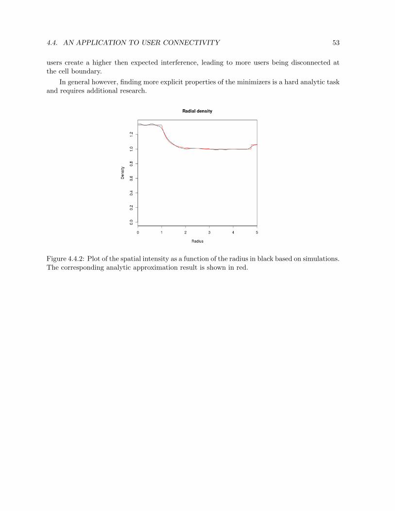
4.4. AN APPLICATION TO USER CONNECTIVITY 53

users create a higher then expected interference, leading to more users being disconnected atthe cell boundary.

In general however, finding more explicit properties of the minimizers is a hard analytic taskand requires additional research.

Figure 4.4.2: Plot of the spatial intensity as a function of the radius in black based on simulations.The corresponding analytic approximation result is shown in red.

Chapter 5

Random malware propagation:the contact process

In contrast to the preceding chapters, where we considered the propagation of wanted messagesover the telecommunication system, we now turn to the propagation of unwanted ones, e.g., ofmalware. We introduce, on the set X of all the device locations, a Markovian time-dependentmodel of the set of infected devices at a given time. The main random mechanism that drivesthis infection has two elements: (1) each user that has an infected neighbor is also infected afteran exponentially distributed random time, and (2) any infected device undergoes a spontaneoushealing after another exponential random time.

This is a well-known mechanism of a Markovian random process on a state space of theform EX, the contact process; every device Xi has two possible states, infected or susceptible.The contact process is a prominent object in the theory of interacting particle systems (IPS). Ina nutshell, it is the theory of continuous-time Markov jump processes on discrete configurationspaces of the form EX, where X carries some neighboring structure, see [L85] for the standardtext book on the subject. The contact process has not yet been investigated, to the best of ourknowledge, on a PPP X, but if the locations of the devices are replaced by the fixed sites in thestandard grid Zd, then there are many precise results in the literature.

The spontaneous healing can be seen as a counter measure that the operator has installedin the system. However, we consider such a model not as the most suitable one for describingthis; rather we would like to introduce a third possible state in the model: to be healthy andimmune for later attacks by the malware. This seems to lead to an IPS that has not yet beenintroduced to the literature yet.

In Section 5.1 we introduce continuous-time Markov chains on finite sets and explain howjump rates characterize the process. The contact process is introduced in Section 5.2, and inSection 5.3 we summarize some of its most important properties in the simpler situation on thegrid Zd in place of X. Finally, in Section 5.4 we give an outlook on related models that mightbe useful in the modeling of propagation of malware in telecommunication systems and still arewaiting for their exploration.

55

56 CHAPTER 5. RANDOM MALWARE PROPAGATION: THE CONTACT PROCESS

5.1 Markov chains in continuous time

Let us explain how a Markov chain in continuous time is characterized and constructed generallyin terms of waiting times and jump rates. We do this here only for a finite set Ω as the state space.Let (ωt)t∈[0,∞) denote a time-homogeneous Markov chain in continuous time on Ω with startingsite ω0 = a. Such a process must be necessarily a jump process. Let τ1 = inft > 0: ωt 6= adenote the first jump time, i.e., the first time at which the particle leaves its initial state. Then,by the Markov property and time-homogeneity,

Pa(τ1 > t+ h|τ1 > t) = Pa(τ1 > t+ h|ωt = a) = Pa(τ1 > h), t, h ∈ (0,∞).

Hence, Pa(τ1 > t+h) = Pa(τ1 > h)Pa(τ1 > t), but this is a functional equation that can only besolved by the exponential function. Thus, Pa(τ1 > t) = exp(−λat), for some λa ∈ (0,∞), whichmeans that τ1 must be exponentially distributed. The parameter λa can be recovered via

− d

dh

∣∣∣h=0

Pa(τ1 > h) = λa.

The decision of the process at the jump times is described by a stochastic matrix p = (pa,b)i,j∈Ω,where pa,b ∈ [0, 1] is the probability to jump from state a to state b. We can neglect pa,a andassume that pa,b be positive only for a 6= b. This is simply the transition matrix of a discrete-time Markov chain that never stands still. But then, for b 6= a we have that Pa(ωτ1) = b) = pa,b.We introduce the jump rates of the process as

c(a, b) = − d

dh

∣∣∣h=0

Pa(ωh = b) = λapa,b ∈ [0,∞). (5.1.1)

The collection of all the jump rates is called the transfer matrix, Q-matrix or generator of theprocess

L = (c(a, b))a,b∈Ω.

Certainly, the further propagation of the Markov process X is done (in accordance with theMarkov property) by iteration of the above described procedure, starting at time τ1 with theprocess at its new location after one jump.

The transfer matrix, together with the initial distribution, characterizes the distribution ofthe process completely. The expected waiting time for a jump is given by λa =

∑b∈Ω\a c(a, b)

and by definition c(a, a) = −λa. In particular, the row sums of L are all equal to zero.

A common way to describe the jump mechanism is in terms of the asymptotics

Pν(ωt+h = b | ωt = a) = 1− c(a, b)h+ o(h), h ↓ 0,

for initial distribution ν on Ω and transfer matrix L.

The paths of the Markov chain (ωt)t∈[0,∞) are right-continuous everywhere and constantstrictly between the jump times and have left limits at the jump times. In other words, thepaths lie in the space of cadlag paths

D[0,∞) = f : [0,∞)→ Ω: f is right-continuous and has left-limits everywhere.

To fix some measurability structure on D[0,∞), we at least want to be able to evaluate theprocess at any given time on the Borel-sigma-algebra on Ω, i.e., we equip D[0,∞) with the

5.2. THE CONTACT PROCESS 57

sigma algebra generated by the events ωt ∈ A for all t ≥ 0 and A ∈ B(Ω), which also providesus with a filtration.

In the simplest case where Ω = N, ω0 = 0 and c(a, b) = q(1b = a + 1 − 1b = a)for all a ∈ N0, the process of jump times is a PPP on [0,∞) with intensity q. The Markovprocess (ωt)t∈[0,∞) increases by one after independent exponential times with parameter q. Sucha process can be used as the counting process for another (time-homogeneous) Markov chain incontinuous time; it ‘rings’ at all the times at which that process must make a jump.

5.2 The contact process

In this section, we consider a particular continuous-time Markov chain with relevance for therandom propagation of malware over a system of devices, the contact process. We first makesome general remarks on interacting particle systems as continuous-time Markov chains withinfinite state space.

Let us keep a locally finite point configuration x = xi : i ∈ I fixed, which can now becountably infinite. We assign to each xi a certain property ωt(xi) ∈ E at time t, where E is afinite set of all the states in which the users xi can be. Rates c(ζ, ξ) are then a priori definedfor any pair of states ζ, ξ ∈ Ω. There is no problem to construct a Markov process, as longas the set x of devices is finite. However, if x is infinite, some serious mathematical problemsin the construction arise, since the state space Ω = Ex is then even uncountably infinite. Thetransition rates can not be simply collected in a transfer matrix anymore, which necessitatesthe use of Markov generators and their associated semigroups, a theory which we will not enterhere. The rates can still be extracted from the distribution via (5.1.1). In order to go the otherway around, namely to construct a process from a given set of rates, one has to employ deepresults from functional analysis, in particular the Hille-Yoshida theorem, for details see [L85].Existence of a process can be guaranteed if the rates satisfy a number of conditions, for examplethat supζ

∑ξ∈Ω c(ζ, ξ) <∞, which prevents the process from having waiting-time distributions

with infinite parameter. Let us note that many IPS can also be constructed by a graphicalrepresentation without the use of generator theory.

In the cases that we want to consider here, we keep things much simpler (and more natural)and requires that the only steps that can be made at a given time are the flips of any of thestates of one xi. Hence, the only non-zero rates c(ζ, ξ) are the ones for ζ and ξ that are distinctin just one site xi. This is already an ad-hoc definition of an interacting particle system (IPS) inthe sense of [L85] (even though the term ‘interacting particle system’ is sometimes understoodin a much wider sense or is used for certain processes of a rather different nature).

One simple way to determine rates for the flip of the state of a given xi from a ∈ E tob ∈ E \ a is to fix it as a constant, not depending on anything else. This is a good choicefor describing a spontaneous healing of an infected device, when a is the infected state andb a healthy state. However, we also want to describe more interesting mechanisms, where aninfection comes from neighbors. The best well-known and perhaps most studied process thatdescribes this is the contact process, which we introduce now.

The contact process is defined on Ω = Ex for E = 0, 1 (‘1’ standing for ‘infected’ and ‘0’for ‘healthy’) and a general countably-infinite site space x = xi : i ∈ I with some neighbor-hood structure. More precisely, we need a notion of two sites being directly connected, usuallyrepresented by an edge between the points. Think for example of the Boolean model, i.e., the in-


fection can jump from device to device if their spatial distance is smaller than a given threshold.More refined models of the underlying graph can also be considered such as the SINR modelintroduced in Section 3.3.

Then, the contact process is characterized by jump rates on Ω of the form c(ζ, ζi), wherethe configuration ζi equals ζ except at the site xi where ζixi = 1− ζxi . Then, for all xi ∈ x,

c(ζ, ζi) =

1, if ζxi = 1,

λ∑

j∈I : xj∼xi 1ζxj = 1, if ζxi = 0,(5.2.1)

and ∼ denotes the neighborhood relation. All other rates c(ζ, ξ) are equal to zero, i.e., onlysingle-site states are changed in a jump. An infected site becomes spontaneously healthy withfixed rate one, independent of all the other sites. On the other hand, a healthy site becomesinfected with a rate that is λ times the number of infected neighbors. The parameter λ > 0 inthe model allows us to tune the strength of the infection. The model has a natural interpretationas to represent a random spread of a disease with an additional self healing component. Notethat a healthy site can again be infected later; there is no possibility of immunization in thismodel.

The contact process defined by the rates in (5.2.1) does belong to the class of models forwhich an infinite-space version is well-defined at least for situations where the underlying graphis a lattice or regular fixed geometry.

5.3 The contact process on Zd

The contact process, although appearing innocent, shows many interesting features already onthe lattice Zd with the usual neighborhood structure. Most prominently, it has a phase transitionwith respect to its class of invariant measures.

Let us first present some general notions for IPSs. We denote by Pν the measure underwhich the IPS is defined with the initial distribution ν on Ω.

Definition 5.3.1 (Invariant measures). A probability measure ν on Ω is called invariant for theIPS if

Pν ω−1t = ν, for all t ≥ 0.

(We use the measure-theoretic notation P X−1 for the distribution of a random variable Xunder a probability measure P.) Moreover, the IPS is called ergodic if it has a unique invariantmeasure ν that satisfies that, for all starting measures ν ′,

limt→∞

Pν′ ω−1

t = ν

in the weak topology.

Invariant measures represent initial distributions that do not change under the evolution ofthe process. Note further that the set of invariant measures is always a convex set and hence itcan be represented by the subset of extremal invariant measures, which are the ones that cannot be represented by a convex combination of other invariant measures.

Now we turn to the special case of the contact process on Zd (i.e., with the state space

Ω = 0, 1Zd) and with parameter λ ∈ (0,∞) as in (5.2.1). Obviously, the delta measure δ0,

5.4. OTHER IPS FOR TELECOMMUNICATIONS 59

which puts mass one on the configuration ω with ωxi = 0 for all xi ∈ x, is invariant under theevolution of the contact process. We have the following theorem.

Theorem 5.3.2. Consider x = Z, then there exists λcr ∈ (0,∞) such that for λ < λcr, thecontact process is ergodic. For λ > λcr the process is not ergodic. In particular, there existinfinitely many additional invariant measures.

Remark 5.3.3 (Properties of the contact process). 1. In the super-critical regime, the set ofinvariant measures is given by convex combinations of δ0 and another invariant measure νλ,usually referred to as the upper invariant measure. It can be defined as limt→∞ Pδ1 ω−1

t =νλ. In this regime, for some starting configurations, the malware can survive for all times.

2. Approximations for the critical rate suggest that λcr ≈ 1.6494, see [L85, page 275].

3. Similar to the percolation probability θ, we can define ρ(λ) = νλ(ζ0 = 1), the probabilitythat the device at the origin is infected under νλ. Again, close to the critical value, thisquantity should behave like a power law with some critical exponent. 3

5.4 Other IPS for telecommunications

The contact process, although defendable as a model for simple telecommunication systems, iscertainly not the most accurate description of malware propagation in such a network. Anotherclassical model that has an interpretation in telecommunications is the voter model, see [L85].Here, q ∈ N different opinions, or viruses, are in the system and the updating is given by

c(ζ, ζi,a) = λ∑

j∈I:xj∼xi

1ζxj = a.

In words, the configuration ζ flips site i into state a with a rate equal to λ times the number ofneighboring sites that have the opinion a.

Let us finally mention some extensions and generalizations that we believe should be inves-tigated in the context of IPS for telecommunications.

Remark 5.4.1 (IPS for telecommunications). 1. The set up of possible states should at leastcomprise a state of susceptibility, a state of infection and a state of immunization. Theimmune state then refers to a device on which an update has been installed.

2. For data protection reasons, the update can only be installed by the operator on an infecteddevice if this device has made its infection obvious on its own, for example by attacking adevice that possesses the healing capability.

3. Users with healing capability, sometimes called white knights, should be placed determin-istically or randomly in the system. Their placement introduces another set of networkparameters, which must be distinguished.

4. The setting of IPS should be extended to cover random geometries. For example, oneshould investigate IPS on realizations of the PPP with a neighborhood structure providedfor example by the Boolean model. Here typically two scenarios are relevant: (1) theannealed setting, where the properties are investigated in expectation of the realizationsof the Boolean model, and (2) the quenched setting, where a typical realization of theBoolean model is fixed in advance hopefully leading to results in the almost sure sense. 3


Let us close this section by giving some illustration of the spread of some malware, startingfrom one infected user at the origin in the setting of a Boolean model for a Cox point process,see Figure 5.4.1.

Figure 5.4.1: Realization of randomly placed users on a street system of Poisson-Voronoi tessel-lation type. The larger green discs indicate randomly placed white knights. Left: initial timewith one infected user in red at the center. Right: some finite time snapshot in which the mal-ware has started to infect surrounding users in red. The green regular size users are vaccinatedby an software update initiated by some contact of the infection with a white knight.

References

[BR06] B. Bollobas and O. Riordan, Percolation, Cambridge University Press, New York(2006).

[Bi68] P. Billingsley, Convergence of Probability Measures, Wiley, New York (1968).

[BB09a] F. Baccelli and B. B laszczyszyn, Stochastic Geometry and Wireless Networks:Volume I: Theory Now Publishers Inc. (2009).

[BB09b] F. Baccelli and B. B laszczyszyn, Stochastic Geometry and Wireless Networks:Volume II: Applications Now Publishers Inc. (2009).

[CHJ17] E. Cali, C. Hirsch and B. Jahnel, Continuum Percolation for Cox processes,Preprint available at arXiv:1710.11407 (2017).

[CSKM13] S.N. Chiu, D. Stoyan, W.S. Kendall and J. Mecke, Stochastic Geometry andIts Applications, J. Wiley & Sons, Chichester (2013).

[DVJ03] D.J. Daley and D. Vere-Jones, An Introduction to the Theory of Point Processes,Vol. I: Elementary Theory and Methods, Second Edition, Springer (2003).

[DZ10] A. Dembo and O. Zeitouni. Large Deviations Techniques and Applications, volume 38of Stochastic Modelling and Applied Probability. Springer (2010). Corrected reprint of thesecond (1998) edition.

[DBT05] O. Dousse, F. Baccelli and P. Thiran Impact of interferences on connectivity inad hoc networks, IEEE/ACM Transactions on Networking (TON) 13, 425–436 (2005).

[DFMMT06] O. Dousse, M. Franceschetti, N. Macris, R. Meester and P. ThiranPercolation in the signal to interference ratio graph, Journal of Applied Probability 43,552–562 (2006).

[FM08] M. Franceschetti and R. Meester, Random Networks for Communication: fromStatistical Physics to Information Systems, Cambridge University Press, Cambridge (2008).

[G61] E.N. Gilbert, Random plane networks, J. of the Society for Industrial & Appl. Math.9, 533–543 (1961).

[G89] G.R. Grimmett, Percolation. New York: Springer-Verlag (1989).

[H12] M. Hanggi, Stochastic Geometry for Wireless Networks, Cambridge University Press,Cambridge (2012).

[HJKP18] C. Hirsch, B. Jahnel, P. Keeler and R. Patterson, Large deviations in relay-augmented wireless networks, Queueing Systems 88:3–4 (2018).

61


[J86] S. Janson, Random coverings in several dimensions, Acta Math. 156, 83–118 (1986).

[K95] J. Kingman, Poisson Processes, Volume 3 of Oxford Studies in Probability, OxfordUniversity Press, Oxford (1995).

[Kl06] A. Klenke, Wahrscheinlichkeitstheorie, Springer, Berlin, 2006.

[LP17] G. Last and M. Penrose, Lectures on the Poisson Process, IMS Textbook, CambridgeUniversity Press, Cambridge (2017).

[L85] T. Liggett, Interacting Particle Systems, New York: Springer-Verlag (1985).

[M75] G. Matheron, Random Sets and Integral Geometry. London: John Wiley & Sons(1975).

[MR96] R. Meester and R. Roy. Continuum Percolation, Cambridge University Press,Cambridge (1996).

[OBSC00] A. Okabe, B. Boots, K. Sugihara and S.N. Chui. Spatial Tessellations: Con-cepts and Applications of Voronoi Diagrams, J. Wiley & Sons, Chichester (2000).

[P91] M.D. Penrose. On a continuum percolation model, Adv. Appl. Probab. 23:3, 536–556(1991).

[P03] M.D. Penrose. Random Geometric Graphs, volume 5 of Oxford Studies in Probability.Oxford University Press, Oxford (2003).

[QZ07] J.A. Quintanilla and R.M. Ziff. Asymmetry in the percolation thresholds of fullypenetrable disks with two different radii, Phys. Rev. E76, 051–115 (2007).

[RS15] F. Rassoul-Agha and T. Seppalainen, A course on large deviation theory with anintroduction to Gibbs measures, Graduate Studies in Mathematics 162, AMS (2015).

[Re87] S.I. Resnick, Extreme Values, Regular Variation and Point Processes, Applied Proba-bility. A Series of the Applied Probability Trust 4. Springer, New York (1987).

[YCG11] C. Yao, G. Chen and T.D. Guo, Large deviations for the graph distance in super-critical continuum percolation, J. Appl. Probab. 48, 154–172 (2011).

Index

τ -convergence, 20τ -topology, 4

annealed, 59asymptotically essentially connected, 38

Boolean model, 23, 24, 27, 45, 59

cadlag path, 56Campbell theorem, 10, 41

refined, 13Campbell-Little-Mecke formula, 14capacity functional, 25

of Boolean model, 26of SINR model, 43

cluster, 28, 30communication area, 3, 24, 27, 50communication zone

local, 24connectivity, 23

of Boolean model, 27of SINR model, 45

contact distance, 9, 15contact process, 55, 57

phase transition, 59on Zd, 58upper invariant measure, 59

contraction principle, 49convergence

τ -, 20in distribution, 20vague, 20weak, 20, 21, 49

counting process, 57covariance

function, 26of counting variables, 10of coverage variables, 26

coverage, 23, 24

probability, 26, 27

Cox point process, 15, 29, 37

Cramer theorem, 49

Cramer transform, 48

degree, 44

directing random measure, 16

empirical mean, 49

empirical measure, 21, 50, 51

generating function, 7

generator, 56

Gilbert graph, 27

Hausdorff measure, 16

high-density limit, 19, 21, 47, 50

LDP, 50

homogeneous random point cloud, 6

independent marking, 11, 24

intensity, 8

intensity measure, 6

absolutely continuous, 8

discrete, 8

interacting particle system, 55, 57

interference, 39, 40

distribution, 40

expectation, 40

Fourier transform, 41

Laplace transform, 41

signal-to-interference cell, 43

signal-to-interference ratio, 42

SINR model, 43

total, 44, 51

invariant measure, 58

IPS, 55, 57

isotropic, 39

distribution, 8

63

64 INDEX

jump process, 56jump rate, 56

Kullback-Leibler divergence, 50

Laplace principle, 50Laplace transform

of Cox point process, 16of interference, 41of interference with signal power, 42of marked Poisson point processes, 11of point processes, 5of Poisson distribution, 7of Radon measures, 21

large-deviations principle, 48, 49LDP, 48, 49Legendre transform, 48locally finite, 4lower semicontinuous, 49

malware, 55Manhattan grid, 18

nested, 18mapping theorem, 10mark, 11

space, 11, 24marked Poisson point process, 11marking

independent, 11, 24theorem, 12

Markov chaincontinuous-time, 9, 56discrete-time, 56ergodic, 58

Markov inequality, 48measurability

of D[0,∞), 56of Boolean model, 24on S(D), 5via vague topology, 20

Mecke-Slivnyak theorem, 15stationary, 15, 29

metrizable, 20

noise, 42

Palm distribution, 13, 29, 43reduced, 14

path-loss exponent, 39path-loss function, 39PDT, 17Peierls argument, 30percolation, 28

Bernoulli bond, 29, 31Bernoulli site, 32, 38continuum, 23, 27critical behavior, 32critical threshold, 29, 30discrete bond, 29for Cox point processes, 37of SINR model, 45probability, 28probability, discrete, 30sub-critical regime, 29super-critical regime, 29, 34

phase transition, 23, 27, 29point measure, 3point process, 3

Cox, 15, 29, 37percolation, 37

Poisson, 3, 6, 8marked, 11

stationary, 8Poisson

distribution, 7limit theorem, 7point process, 3, 6, 8standard point process, 8superposition principle, 8

Poisson-Delaunay tessellation, 17Portmanteau theorem, 5PPP, 3, 57PVT, 17, 38

stabilizing, 19

Q-matrix, 56quenched, 59

Radon measure, 4, 6, 20random, 20

random closed set, 16, 24, 25, 27random environment, 16random field

absolutely continuous, 16Bernoulli, 29

random geometric graph, 27

INDEX 65

random measure, 16random point measures

sequences, 20rate function, 49

good, 50relative compactness, 20relative entropy, 50renewal process, 18

scale invariant measure, 29segment process, 16shape theorem, 36shift invariant

measure, 8shift invariant random point cloud, 6shot noise, 16signal power, 42SINR, 42SINR model, 43–45, 58SIR, 42, 51stabilization, 18, 37

radius, 18stabilizing measure, 18stationary

Boolean model, 26Markov chain, 56point process, 8random point cloud, 6

street system, 16stretch factor, 36superposition principle, 8, 9

tessellation, 17Manhattan grid, 18nested Manhattan grid, 18Poisson line process, 18Poisson-Delaunay, 17Poisson-Voronoi, 17, 38, 60Poisson-Voronoi cell, 24

thinning, 9topology

τ -, 4on mark space, 11vague, 4

transfer matrix, 56transition matrix, 56transmission strength, 42two-point connectivity, 34

uplink, 52

vague convergence, 20vague topology, 4Varadhan’s lemma, 50volume fraction, 26voter model, 59

weak convergence, 20, 49white knight, 59

probabilistic methods in telecommunication

Documents