probabilistic adequacy and measures
TRANSCRIPT
NERC | Report Title | Report Date I
Probabilistic Adequacy and Measures Technical Reference Report Final July, 2018

NERC | Probabilistic Adequacy and Measures Report| July, 2018 ii
Table of Contents
Preface ...................................................................................................................................................................... iv
Executive Summary .................................................................................................................................................... v
Objectives ............................................................................................................................................................... v
Survey Objectives: .............................................................................................................................................. v
Key Findings ........................................................................................................................................................... vi
General Recommendations ................................................................................................................................... vi
Detailed Recommendations on RRMs .................................................................................................................. vii
Introduction ............................................................................................................................................................ viii
Background .......................................................................................................................................................... viii
NERC Survey on Probabilistic Studies .................................................................................................................. viii
Chapter 1: Reliability Risk Metrics ............................................................................................................................. 1
Basic Computational Approaches ........................................................................................................................... 1
Loss of Load Hours .................................................................................................................................................. 2
Definition ............................................................................................................................................................ 2
Methods for Calculation-Computation Methods ............................................................................................... 2
Loss of Load Events ................................................................................................................................................ 3
Definition ............................................................................................................................................................ 3
Methods for Calculation-Computation Methods ............................................................................................... 4
Considerations on the Use of LOLEV .................................................................................................................. 4
Loss of Load Expectation ........................................................................................................................................ 4
Definition ............................................................................................................................................................ 4
Methods for Calculation-Computation Methods ............................................................................................... 4
Considerations on the Use of LOLE ..................................................................................................................... 5
Loss of Load Probability .......................................................................................................................................... 6
Definition ............................................................................................................................................................ 6
Methods for Calculation-Computation Methods ............................................................................................... 6
Considerations on the Use of LOLP..................................................................................................................... 7
Expected Unserved Energy ..................................................................................................................................... 7
Definition ............................................................................................................................................................ 7
Methods for Calculation-Computation Methods ............................................................................................... 7
Considerations and Recommendations on the Use of EUE ................................................................................ 7
Summary of Reliability Risk Metrics ....................................................................................................................... 7
Chapter 2: Applications .............................................................................................................................................. 9
Table of Content
NERC | Probabilistic Adequacy and Measures Report | July, 2018 iii
LOLP .................................................................................................................................................................... 9
EUE ...................................................................................................................................................................... 9
LOLH .................................................................................................................................................................... 9
LOLE .................................................................................................................................................................... 9
LOLEV ................................................................................................................................................................ 10
Chapter 3: Probabilistic Studies Assessing Emerging Reliability Issues ................................................................... 11
The Use of Probabilistic Studies to Assess Emerging Issues ................................................................................. 11
Industry Application of Reliability Metrics into Emerging Issues ......................................................................... 13
Loss of Load Probability ........................................................................................................................................ 13
Expected Unserved Energy ................................................................................................................................... 13
Loss of Load Expectations..................................................................................................................................... 13
Loss of Load Expected Events ............................................................................................................................... 13
Loss of Load Hours ................................................................................................................................................ 14
Conclusions .............................................................................................................................................................. 15
Appendix A: Survey Building Blocks ......................................................................................................................... 16
Appendix B: Survey Questions ................................................................................................................................. 18
Appendix C: Reliability Risk Metrics Calculations Monte Carlo Approach ............................................................... 23
Appendix D: Reliability Risk Metrics Calculations—Analytical Approach ................................................................ 28
Appendix E: Additional Resource Adequacy Metric ................................................................................................ 38
NERC | Probabilistic Adequacy and Measures Report| July, 2018 iv
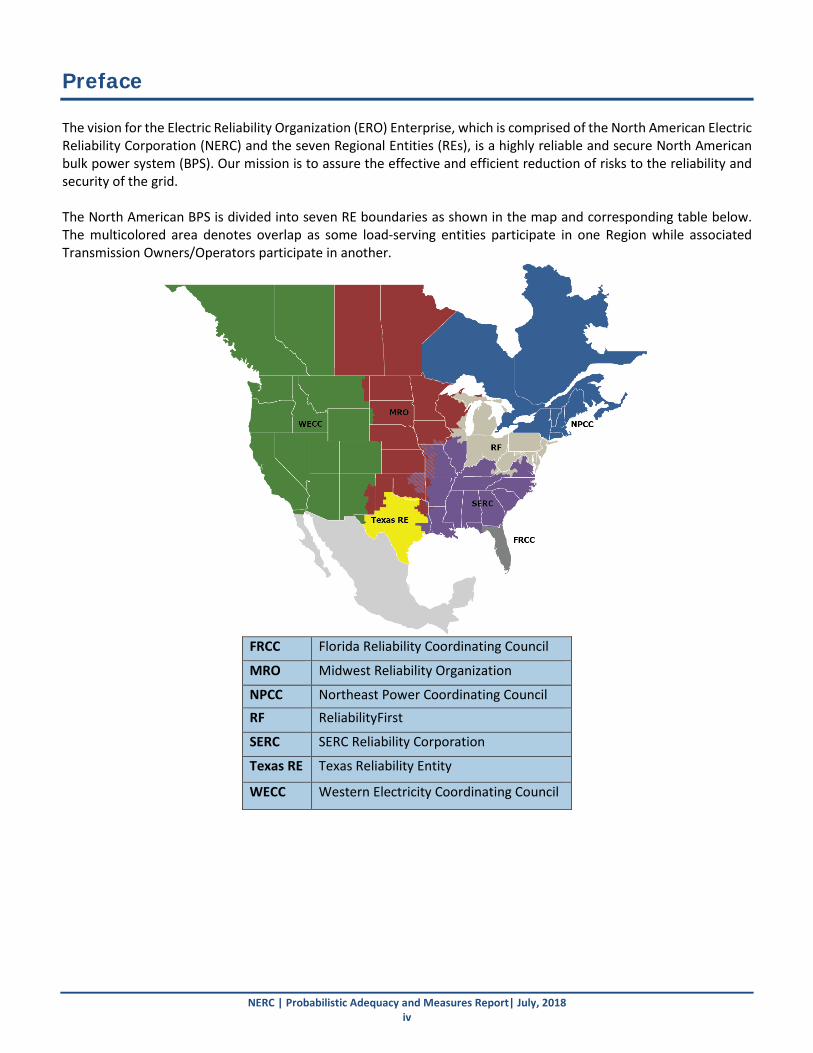
Preface The vision for the Electric Reliability Organization (ERO) Enterprise, which is comprised of the North American Electric Reliability Corporation (NERC) and the seven Regional Entities (REs), is a highly reliable and secure North American bulk power system (BPS). Our mission is to assure the effective and efficient reduction of risks to the reliability and security of the grid. The North American BPS is divided into seven RE boundaries as shown in the map and corresponding table below. The multicolored area denotes overlap as some load-serving entities participate in one Region while associated Transmission Owners/Operators participate in another.
FRCC Florida Reliability Coordinating Council
MRO Midwest Reliability Organization
NPCC Northeast Power Coordinating Council RF ReliabilityFirst
SERC SERC Reliability Corporation
Texas RE Texas Reliability Entity
WECC Western Electricity Coordinating Council

NERC | Probabilistic Adequacy and Measures Report| July, 2018 v
Executive Summary NERC assesses current and future adequacy and operational reliability of the North American BPS through seasonal, long-term, and short-term special assessments. These assessments inform policy makers and regulators of emerging issues and potential concerns by identifying notable trends impacting the North American BPS. The electric power industry is undergoing significant and rapid change, increasing the need for more probabilistic approaches. NERC recognizes that these emerging issues are highly variable and uncertain and can have an effect on traditional resource adequacy assessments. NERC is considering the value of implementing more probabilistic approaches to measuring BPS resource and transmission adequacy and evaluating whether probabilistic approaches should be used permanently in resource adequacy/reliability assessments. The NERC Probabilistic Assessment Working Group (PAWG) was assigned to review the use of probabilistic studies in assessing these emerging reliability risks and produce this report. This report covers the work done by NERC, the Planning Committee (PC), the Reliability Assessment Subcommittee (RAS), and the PAWG in supporting this needed review. Objectives NERC’s goals in developing this report are as follows:
• Develop a collective understanding of existing applications of probabilistic techniques used for reliability assessments and planning studies.
• Identify emerging reliability issues for which probabilistic studies are likely to provide significant insights.
• Review existing reliability risk metrics (RRMs), provide a common understanding of their definitions and use, and recommend future enhancements and applications.
• Identify commonalities to inform industry on the applications of probabilistic reliability metrics.
• Provide guidance on the development of probabilistic methods for ensuring resource adequacy and reliability to allow better risk-informed decisions for planners and policy makers in the face of increasing uncertainty of supply and demands on the BPS.
The foundation of the report is based on results from a NERC survey on probabilistic studies as well as data and information gathered by NERC from Regions and assessment areas. Survey Objectives:
• Review the ongoing probabilistic analyses and future plans for further insights into resource adequacy assessment.
• Understand the choice of probabilistic methods, tools, and selection of acceptable reliability levels used by NERC Regions and the industry at large to assess resource and transmission adequacy.
• Show the need to expand probabilistic studies to help assess emerging reliability issues that have an impact on BPS reliability.
• Explore the probabilistic approaches used that provide further insights into how to best establish adequate reserve margins amidst a BPS undergoing unprecedented changes.
• Identify how members of industry define and apply RRMs.

Executive Summary
NERC | Probabilistic Adequacy and Measures Report | July, 2018 vi
• Explore applications of commonly used RRMs and how each RRM can measure different aspects of a system’s reliability (e.g., frequency, duration, and magnitude of loss of load), depending on how the metric is defined and applied.
• Provide recommendations on the application of commonly used RRMs in assessing system adequacy. Key Findings
• There are variations in how a reliability criterion is defined and interpreted in existing practices in the assessment areas across the United States and Canada.
• The majority of entities in North America conducting resource adequacy studies primarily use the loss of load expectation (LOLE) metric to establish a single resource adequacy criterion. In turn, the LOLE RRM generally helps inform integrated resource planning, market-based resource procurement, generator interconnection queue projects, and other planning activities.
• About one third of survey respondents use the expected unserved energy (EUE) metric for assessing reliability. EUE provides insight to the impact of energy limited resources on a system’s reliability, particularly in systems with growing penetration of such resources. Examples of such energy limited resources include the following:
Demand response programs can be modeled as resources with specific contract limits, including hours per year, days per week, and hours per day constraints.
Energy efficiency programs can be modeled as reductions to load with an hourly load shape impact.
DERs, such as behind the meter solar photovoltaic, can be modeled as reductions to load with an hourly load shape impact
• The choice of probabilistic methods and selection of acceptable adequacy levels are still matters of judgment and differ from Region to Region and from assessment area to assessment area and even utility to utility in some cases.
• Most assessment areas are already using or are considering probabilistic approaches to assess emerging reliability issues.
• There is a recognized need to support probability-based resource adequacy assessment resulting from the changing resource mix with significant increases in variable and energy-limited resources (intermittent in nature), changes in net demand profiles resulting in the shifting of the hour of the peak demand, and other factors that can have an effect on resource adequacy.
• A number of issues based on industry survey results are out of the PAWG scope of work and therefore are not discussed in this report. These issues are as follows: operational concerns, such as unit commitment; over-generation and dispatch issues; essential reliability service issues, such as VER capacity credit evaluation, ramping, flexibility, and regulations; and potential resource upgrades.
General Recommendations The RAS agrees with the PAWG recommending the following:
• Entities may leverage other metrics and factors in their criteria development to determine a sufficient reserve margin to maintain an adequate level of system reliability, especially for systems with a diverse generation mix and VERs.
• NERC should continue to incorporate more probabilistic approaches into its assessments and continue to review and provide guidance on the development of probabilistic methods for ensuring resource adequacy and reliability.

Executive Summary
NERC | Probabilistic Adequacy and Measures Report | July, 2018 vii
• NERC should continue conducting periodic reviews on RRMs and criteria used to assure they are clear and properly structured for existing and emerging risks.
• As entities and system planners identify emerging reliability issues or large changes on their system (e.g., change in size, resource mix, etc.), they should evaluate whether the incorporation of additional RRMs could improve their assessment of risks to reliability.
Detailed Recommendations on RRMs The RAS agrees with the PAWG recommending the following:
Loss of Load Hours The PAWG recommends the use of loss of load hours (LOLH) RRM using all hours rather than just peak periods for both small and large systems. It can be evaluated over seasonal, monthly, or weekly study horizons. LOLH does not inform of the magnitude or the frequency of loss of load events; it is used as a measure of their combined duration. LOLH is applicable to both large and small systems and is relevant for assessments covering all hours (compared to only the peak demand hour of each season). LOLH provides insight to the impact of energy limited resources on a system’s reliability, particularly in systems with growing penetration of such resources. Examples of such energy-limited resources include the following:
• Demand response programs, which can be modeled as resources with specific contract limits including hours per year, days per week, and hours per day constraints
• Energy efficiency programs, which can be modeled as reductions to load, with an hourly load shape impact
• Distributed resources, such as behind the meter PV, which can be modeled as reductions to load, with an hourly load shape impact
Loss of Load Expected Events PAWG recommends loss of load expected events (LOLEV) to be used alongside other metrics specified in this report when evaluating capacity planning decisions. This is more for systems where planners are concerned about the potential for multiple loss of load events in a single day. Loss of Load Expectation For LOLE RRM, PAWG recommends the following:
• Entities evaluate all hours of a given time period when calculating LOLE, especially considering the impact a changing resource mix (particularly DERs and VERs) is having on the daily load distributions of many areas across the BPS.
• Entities to report the time period and hours associated with their LOLE calculation and the reasoning behind their approach for instance, the LOLE evaluated on just the daily peak hours will always be equal to or less than an LOLE based on all hours.
Expected Unserved Energy With the changing generation mix and to make EUE a more effective metric, PAWG recommends the following:
• Hourly EUE values should be reported for every month or year (i.e., 24 data points), as this is the only metric which considers magnitude of loss of load events.
• System planners estimate the cost and impact of the loss of load events by using EUE as it is a useful measure to estimate the size of loss of load events and can be used as basis for the reference reserve margin to determine capacity credits for VERs.
• For extreme weather conditions and common mode failure events, PAWG recommends using EUE RRM as this measure quantifies events impacts on system reliability.
NERC | Probabilistic Adequacy and Measures Report| July, 2018 viii
Introduction NERC recognizes that such factors as the changing resource mix, shifting demands, and other factors can have a significant effect on resource adequacy. As a result, NERC is incorporating more probabilistic approaches and other ongoing analyses to provide further insights on how to best establish adequate reserve margins and analyze other reliability issues. While NERC has historically gauged resource adequacy by using deterministic planning reserve margins, it is now exploring the expanded use of probabilistic approaches to support resource adequacy analysis. Background In the continuing effort to improve NERC’s probabilistic and deterministic assessments, the now-disbanded Probabilistic Assessment Improvement Task Force (PAITF) formed in May 2015 to identify improvement opportunities for NERC’s Long-Term Reliability Assessment (LTRA) and complementary probabilistic analysis. The PAITF defined five different widely used probabilistic resource adequacy statistics, such as LOLE, LOLH, EUE, loss of load probability (LOLP), and LOLEV. Only LOLH and EUE have been reported in past NERC Core Probabilistic Assessment reports for all assessment areas.1, 2, 3 Advancing further effort towards advocating probabilistic adequacy studies, NERC formed the Probabilistic Assessment Working Group (PAWG) in December 2016 with a primary function to further advance the work initiated by the Generation and Transmission Reliability Modeling Task Force (GTRPMTF)4 and the PAITF5 for improving NERC’s Core probabilistic assessments. Given the evolving landscape of resource mix, this technical reference report focuses on identifying, defining, and evaluating more probabilistic approaches and risk metrics for ongoing analyses in order to provide further insights into resource adequacy assessment. This report explores the approaches and applications of commonly used RRMs. The foundation of the report is based on results from a NERC survey on probabilistic studies. 6 In particular, the report presents survey results to the electricity sector on existing and future use of probabilistic studies to investigate BPS risks to reliability and results on tracking evolving emerging reliability trends. The report also recommends applications for the electricity sector to use known reliability metrics to assess emerging issues. NERC Survey on Probabilistic Studies In May 2017, the NERC PAWG distributed a survey on probabilistic studies to seek information on probabilistic approaches adopted by NERC Regions and assessment areas, Balancing Authorities and other industry entities in North America. The RRMs, applications, and probabilistic studies used to assess emerging reliability issues discussed in this report are based on the responses received from more than 70 survey participants in North America.7 Survey objectives are listed on the executive summary of the report.
3 Probabilistic Assessment Improvement Task Force - Technical Guideline Document 2 Probabilistic Assessment Improvement Task Force 3 NERC 2016 ProbA Report 4 See: http://www.nerc.com/docs/pc/gtrpmtf/GTRPMTF%20Meth%20&%20Metrics%20Report%20final%20w.%20PC%20approvals,%20revisions.pdf 5 Probabilistic Assessment Improvement Task Force website. 3 Probabilistic Assessment Improvement Task Force - Technical Guideline Document 7 More survey background information, along with the Probabilistic Studying Survey form, is included in the report as Appendices A and B.

NERC | Probabilistic Adequacy and Measures Report| July, 2018 1
Chapter 1: Reliability Risk Metrics Reliability risk metrics (RRMs) are key considerations for reliability risk planning. RRMs allow system planners to better identify future needs and tailor their decisions accordingly. This chapter discusses common probabilistic RRMs used; basic computational approaches used in RRM calculations; and some considerations on their definitions, modeling, and use. Planners need to accurately forecast the optimum level of resources. In addition to assessing the risk to reliability, planners may also consider the financial cost and environmental burden of their decisions. In turn, this drives methods of how to ensure an adequate level of supply, such as technology type, market designs, or additional market transactions with neighboring systems. Basic Computational Approaches Generally, the probabilistic reliability indices of a system can be evaluated using one of the following two basic approaches: the Monte Carlo simulation or the Convolution Method. The calculation of probabilistic reliability indices is done using either the Monte Carlo simulation or the Convolution method (analytical method). The following is a brief discussion of these two approaches and the static versus short term reserve: Monte Carlo Simulation: The Monte Carlo simulates the actual process and random behavior of the system—treated as a series of experiments. Monte Carlo simulation approaches can be categorized as "non-sequential" and "sequential." A non-sequential simulation process does not move through time chronologically or sequentially, but rather takes only the snap shot of the system state at various time. Non-sequential Monte Carlo simulation is also called state sampling approach. A sequential Monte Carlo simulation steps through the model year chronologically, recognizing the fact that the status of a piece of equipment is not independent of its status in adjacent hours; it tries to simulate the failure and repair history of system components based on their probability distributions of their state residence time. Equipment forced outages are modeled by taking the equipment out of service for contiguous hours, with the length of the outage period being determined from the equipment’s mean-time-to-repair statistics. In both a “non-sequential” and “sequential” Monte Carlo simulation, the number of artificial history replications must be established to achieve an acceptable level of statistical convergence. The degree of statistical convergence of a reliability index is measured by the standard deviation of the estimate of the reliability. Annual indices covering the period of interest are calculated as the average of the accumulated (replication) data until the variance is equal to or smaller than the selected convergence criteria. The “sequential” Monte Carlo simulation requires more input parameters and computation time than the “non-sequential” simulation. However, the sequential simulation can model issues of concern that involve time correlations, such as unit starting times or deferred unplanned outages, and can be used to calculate indices such as frequency and duration. Analytical Method (Convolution): The analytical method for computing resource adequacy indices consists of three steps: 1) the development of the load model which describes the expected system load with uncertainty representation to capture the variation of the demand associated with the weather and or economic forecast, 2) the development of the capacity model which describe the random behavior of the capacity resource outages and the energy generation of the intermittent resources, and 3) the use of probabilistic mathematics to compute the reliability indices associated with the combination of the load and the capacity models. Mathematically, the combination of load and capacity models to compute reliability indices involves the calculation of the distribution of the difference of two random variables. If the random variables are continuous, the probability density function of their sum/difference can be obtained using the convolution integral. Evaluation

Chapter 1: Reliability Risk Metrics
NERC | Probabilistic Adequacy and Measures Report | July, 2018 ii
of convolution integral is very tedious and sometimes there may not exist an analytical solution and therefore approximate methods such as the cumulant methods are used. In this situation, the process of convolution is replaced by finding the summation of the cumulants of the distributions. If the random variables are discrete, the mean values of their sum/difference can be evaluated easily using the discrete convolution method. Some efficient discrete convolution approaches have been developed, such as recursive unit addition and equivalent load approaches. The computation time for these calculations is much faster than the Monte Carlo simulation. Monte Carlo approach becomes more suitable when the analysis includes the interface limit between the subareas. The problem is then modeled as a probabilistic flow network and becomes a highly multidimensional problem. So in the multi-area reliability analysis involving transmission interfaces, the Monte Carlo approach or the hybrid Monte Carlo/Convolution approach is usually required. The following are definitions of commonly used RRMs that can be produced for different time intervals. Some RRMs are best suited for determining static or long term reserve needs. Short term or dynamic reserve8 needs are not typically identified using RRMs. The core of evaluating system reliability is quantifying the amount of demand not served (or loss of load). Demand not served at hour i in the kth Monte Carlo iteration is defined in Equation 1 as follows:
𝐷𝐷𝐷𝐷𝐷𝐷𝑘𝑘𝑘𝑘 = 𝑚𝑚𝑚𝑚𝑚𝑚�0 , 𝐿𝐿𝑘𝑘 − ∑ 𝐺𝐺𝑗𝑗𝑘𝑘𝑚𝑚𝑗𝑗=1 � (1)
Where 𝐿𝐿𝑘𝑘 is the load in hour i, 𝐺𝐺𝑗𝑗𝑘𝑘is the available capacity of the jth generator in the kth sampling (Monte Carlo iteration), and m is the number of generators in the system. 𝐷𝐷𝐷𝐷𝐷𝐷𝑘𝑘𝑘𝑘 is the amount of demand not supplied in hour i, in the kth iteration (in MW). Iki is a Boolean variable representing whether there is demand not supplied in hour i, in the kth iteration using the following definition:
𝐼𝐼𝑘𝑘𝑘𝑘(𝐷𝐷𝐷𝐷𝐷𝐷𝑘𝑘𝑘𝑘) = �0 𝑖𝑖𝑖𝑖 𝐷𝐷𝐷𝐷𝐷𝐷𝑘𝑘𝑘𝑘 = 01 𝑖𝑖𝑖𝑖 𝐷𝐷𝐷𝐷𝐷𝐷𝑘𝑘𝑘𝑘 ≠ 0 (2)
Below are definitions of the common RRMs used in industry for reliability assessments. Loss of Load Hours Definition LOLH is generally defined as the expected number of hours per time period (often one year) when a system’s hourly demand is projected to exceed the generating capacity. This metric is calculated using each hourly load in the given period (or the load duration curve). Methods for Calculation-Computation Methods LOLH is calculated in two steps:
1. Count the number of hours where there is loss of load in each iteration, Equation 3.
2. Average the number of hours (from step 1) across all iterations, Equation 4.
8 Dynamic or short term reserve is a reserve requirement that changes according to the size of the largest contingency or the two largest contingencies the operator is trying to protect.

Chapter 1: Reliability Risk Metrics
NERC | Probabilistic Adequacy and Measures Report | July, 2018 iii
Monte-Carlo These two steps are shown in the equation below:
𝐿𝐿𝐿𝐿𝐿𝐿𝐿𝐿𝑘𝑘 = ∑ 𝐼𝐼𝑘𝑘𝑘𝑘𝐻𝐻𝑘𝑘=1 (3)
Where 𝐿𝐿𝐿𝐿𝐿𝐿𝐿𝐿𝑘𝑘 is the loss of load duration (in hours) in the kth iteration, i is a variable representing each hour, H is the total number of hours in the study period such as 8760, and 𝐼𝐼𝑘𝑘𝑘𝑘 is a Boolean variable representing whether there is demand not supplied in hour i, in the kth iteration. LOLH can be then calculated as shown in equation (4):
𝐿𝐿𝐿𝐿𝐿𝐿𝐿𝐿 = 1𝑁𝑁∑ 𝐿𝐿𝐿𝐿𝐿𝐿𝐿𝐿𝑘𝑘𝑁𝑁𝑘𝑘=1 (4)
Where k is an index representing an iteration, and N is the total number of iterations. Analytical The analytical method used to determine the hourly LOLP for each hour i of the study period can be described by the following formula:
𝐿𝐿𝐿𝐿𝐿𝐿𝐿𝐿 = ∑ 𝐿𝐿𝐿𝐿𝐿𝐿𝐿𝐿𝑘𝑘𝐻𝐻
𝑘𝑘=1 (5) Where i is variable representing each hour, H is the total number of hours in the study period such as 8760, and 𝐿𝐿𝐿𝐿𝐿𝐿𝐿𝐿𝑘𝑘 is the LOLP in hour i. Equation (5) is also valid in a Monte-Carlo context, provided that 𝐿𝐿𝐿𝐿𝐿𝐿𝐿𝐿𝑘𝑘 = 1
𝑁𝑁∑ 𝐼𝐼𝑘𝑘𝑘𝑘𝑁𝑁𝑘𝑘=1 .
Classic analytic calculations would use monthly or annual random variable distributions for which these equations would not work. Appendix C-2 shows an example of LOLP calculation. Considerations on the Use of LOLH LOLH should be evaluated using all hours, rather than just peak periods; it can be evaluated over seasonal, monthly, or weekly study horizons. LOLH does not inform of the magnitude or the frequency of loss of load events, but it is used as a measure of their combined duration. LOLH is applicable to both small and large systems and is relevant for assessments covering all hours (compared to only the peak demand hour of each season). LOLH provides insight to the impact of energy limited resources on a system’s reliability, particularly in systems with growing penetration of such resources. Examples of such energy limited resources include the following:
• Demand response programs, which can be modeled as resources with specific contract limits including hours per year, days per week, and hours per day constraints
• Energy efficiency programs, which can be modeled as reductions to load, with an hourly load shape impact
• Distributed resources, such as behind the meter PV, which can be modeled as reductions to load, with an hourly load shape impact
Loss of Load Events Definition LOLEV, also known as loss of load frequency, is defined as the number of events in which system load is not served in a given time period. A LOLEV counts the expected frequency of continuous LOLH.

Chapter 1: Reliability Risk Metrics
NERC | Probabilistic Adequacy and Measures Report | July, 2018 iv
Methods for Calculation-Computation Methods LOLEV is calculated on all hours, not just daily peak hours. Both Monte Carlo and Convolution methods can be used for evaluating this metric. The risk metric is evaluated using the following formula in Monte Carlo simulation:
𝐿𝐿𝐿𝐿𝐿𝐿𝐿𝐿𝐿𝐿 = 1𝑁𝑁∑ 𝐿𝐿𝐿𝐿𝐿𝐿𝑘𝑘𝑁𝑁𝑘𝑘=1 (6)
Where LLOk is the total number of loss of load occurrences, k is an index representing each iteration, and N is the total number of iterations.
Considerations on the Use of LOLEV LOLEV does not reflect magnitude or duration of loss of load but rather counts how many loss of load events occurred for a consecutive amount of hour(s) in a given time period. LOLEV is useful if considered alongside other metrics specified in this report when evaluating capacity planning decisions. For example, a system where the LOLH and LOLEV are approximately equal would indicate that most events are short in duration, more precisely LOLH and LOLEV are the average duration of outages. LOLEV does not take into consideration the duration or magnitude of the individual involuntary load shed events. The LOLEV metric does not differentiate between events that last for one hour, several continuous hours, or an event where the loss of load is for one or several hundred megawatts of load. Note that this is not a probability index, but a frequency of occurrence index. The LOLEV is also useful for systems where planners are concerned about the potential for multiple loss of load events in a single day. Other metrics, such as LOLE, cannot capture the risk associated with multiple events over the course of a given interval, typically a day. Multiple LLO events are much more likely to occur with significant addition of VERs. As a result, resource planners may underestimate the potential for loss of load events. Loss of Load Expectation Definition LOLE is defined as the expected number of days per time period (usually a year) for which the available generation capacity is insufficient to serve the demand at least once per day. LOLE counts the days having loss of load events, regardless of the number of consecutive or nonconsecutive loss of load hours in the day. Industry experts utilize various techniques from evaluating only the daily peak hour, subset of daily hours, or all daily hours. More on this topic under the Considerations on the Use of LOLE section on the next page. Methods for Calculation-Computation Methods Using a Monte-Carlo technique, the calculation equations are as shown below:
LOLE days/day = 1𝑁𝑁∑ [1
𝐷𝐷∑ 𝐿𝐿𝑘𝑘,𝑑𝑑]𝐷𝐷𝑑𝑑=1
𝑁𝑁𝑘𝑘=1 (7.1)
LOLE days/period = 1𝑁𝑁∑ ∑ 𝐿𝐿𝑘𝑘,𝑑𝑑
𝐷𝐷𝑑𝑑=1
𝑁𝑁𝑘𝑘=1 (7.2)
Where 𝑑𝑑 is a variable representing a day, 𝐷𝐷 is the total number of days, 𝑘𝑘 is a variable representing an iteration, 𝐷𝐷 is the total number of iterations, and 𝐿𝐿𝑘𝑘,𝑑𝑑 is a Boolean variable describing whether there was at least one hour of loss of load in the day:
𝐿𝐿𝑘𝑘,𝑑𝑑 = �0 𝑖𝑖𝑖𝑖 𝐿𝐿𝐿𝐿𝐿𝐿𝐿𝐿𝑘𝑘,𝑑𝑑 = 01 𝑖𝑖𝑖𝑖 𝐿𝐿𝐿𝐿𝐿𝐿𝐿𝐿𝑘𝑘,𝑑𝑑 ≠ 0 (8)
Chapter 1: Reliability Risk Metrics
NERC | Probabilistic Adequacy and Measures Report | July, 2018 v
Where 𝐿𝐿𝐿𝐿𝐿𝐿𝐿𝐿𝑘𝑘,𝑑𝑑 is the loss of load duration for a day for each iteration, shown below is the calculation equation:
𝐿𝐿𝐿𝐿𝐿𝐿𝐿𝐿𝑘𝑘,𝑑𝑑 = ∑ 𝐼𝐼𝑘𝑘𝑘𝑘𝐻𝐻𝑑𝑑𝑘𝑘=1 (9)
Where 𝑖𝑖 is a variable representing each hour, and 𝐼𝐼𝑘𝑘𝑘𝑘 is a Boolean variable representing whether there is demand not supplied in hour i, in the kth iteration, and 𝐿𝐿𝑑𝑑 is the total number of hours in a day being evaluated. Analytical Technique Using an analytical technique, the LOLE can be calculated using the equation below:
LOLE = ∑ max [𝑘𝑘=1𝐻𝐻𝐷𝐷𝑑𝑑=1 (𝐿𝐿𝐿𝐿𝐿𝐿𝐿𝐿𝑘𝑘)])] (10)
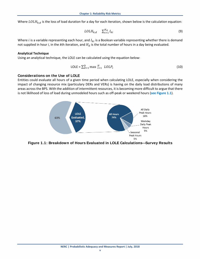
Considerations on the Use of LOLE Entities could evaluate all hours of a given time period when calculating LOLE, especially when considering the impact of changing resource mix (particulary DERs and VERs) is having on the daily load distributions of many areas across the BPS. With the addition of intermittent resources, it is becoming more difficult to argue that there is not liklihood of loss of load during unmodeled hours such as off-peak or weekend hours (see Figure 1.1).
Figure 1.1: Breakdown of Hours Evaluated in LOLE Calculations—Survey Results

Chapter 1: Reliability Risk Metrics
NERC | Probabilistic Adequacy and Measures Report | July, 2018 vi
Based on the Probabilistic Survey Study results, 74 percent of entities using LOLE evaluate all hours (8,760 hours/year), while 16 percent only evaluate the daily peak hours (365 hours/year). The remaining 10 percent consists of two entities, one of which excludes daily peaks on weekends and the other only evaluates the summer and winter peak hour. Also, to allow easy comparison between entities, it is recommended that entities report the time period and hours associated with their LOLE calculation and the reasoning behind their approach. For instance, the LOLE evaluated on just the daily peak hours will always be equal to or less than an LOLE based on all hours. System characteristics, such as the kurtosis (relative peakiness) of the daily load profile, hourly generator performance, and other factors, determines the magnitude of the delta between the two LOLE calculations. This is illustrated using a generic system example shown in Appendix B, where one iteration (#5) did not have loss of load during the peak hour. This iteration impacts the LOLE daily peak hours vs. all hours calculations. In this case, the all hours LOLE of 2 is greather than the daily peak hours LOLE of 1.8. Loss of Load Probability Definition This is defined as the probability of system daily peak or hourly demand exceeding the available generating capacity during a given period. The probability can be calculated either by using only the daily peak loads (or daily peak variation curve) or all the hourly loads (or the load duration curve) in each study period. Methods for Calculation-Computation Methods A Monte-Carlo based approach is based on the mathematical process of random sampling from the generation availability and demand distributions and reiterating the process to determine how many times there is a loss of load. The number of Loss of Load events divided by the number of possible Loss of Load events is the calculation of LOLP. Formula (Using Monte-Carlo Sampling):
1. Assume Gjk is the available capacity of the jth generator in the kth sampling, and m is the number of generators in the system;
System Available Capacity = ∑=
m
jjkG
1
(11)
2. Li is the load at the ith hour;
iL
3. Demand not supplied 𝐷𝐷𝐷𝐷𝐷𝐷𝑘𝑘,𝑘𝑘 in the kth sampling; If Load is less than System Available Capacity this equation will equal 0.
𝐷𝐷𝐷𝐷𝐷𝐷𝑘𝑘,𝑘𝑘 = 𝑚𝑚𝑚𝑚𝑚𝑚�0, 𝐿𝐿𝑘𝑘 − ∑ 𝐺𝐺𝑗𝑗𝑘𝑘𝑚𝑚𝑗𝑗=1 � (12)
4. If Load is greater than Generation Availability, set 𝐼𝐼𝑘𝑘,𝑘𝑘 = 1, otherwise 0;
𝐼𝐼𝑘𝑘,𝑘𝑘 = 𝑚𝑚𝑚𝑚𝑚𝑚 �0,𝐿𝐿𝑘𝑘 �0 𝑖𝑖𝑖𝑖 𝐷𝐷𝐷𝐷𝐷𝐷𝑘𝑘,𝑘𝑘 = 0 1 𝑖𝑖𝑖𝑖 𝐷𝐷𝐷𝐷𝐷𝐷𝑘𝑘,𝑘𝑘 ≠ 0� (13)
Chapter 1: Reliability Risk Metrics
NERC | Probabilistic Adequacy and Measures Report | July, 2018 vii
5. N is the number of replications; LOLP is the count of the times load is greater than availability divided by the number of samplings:
𝐿𝐿𝐿𝐿𝐿𝐿𝐿𝐿 = 1𝑁𝑁∑ 𝐼𝐼𝑘𝑘𝐾𝐾𝑘𝑘=1 (14)
Reviewing the formulas above, it is important to note that the LOLP calculation using a Monte-Carlo approach is a count of how many test periods produce a loss of load in each sample. Therefore, the calculation is highly dependent on what periods are being analyzed.
Considerations on the Use of LOLP LOLP can be calculated for any study period based on numerous time increments of the study period. Either way, the calculation is the same, the count of the periods with loss of load divided by the total number of periods in each sample.
Expected Unserved Energy Definition The EUE is the summation of the expected number of megawatt hours of demand that will not be served in a given time period as a result of demand exceeding the available capacity across all hours. EUE is an energy-centric metric that considers the magnitude and duration for all hours of the time period, calculated in megawatt hours (MWh). This measure can be normalized based on various components of an assessment area (e.g., total of peak demand, Net Energy for Load, etc.). Normalizing the EUE provides a measure relative to the size of a given assessment area. One example of calculating a Normalized EUE part per million or ppm is defined as follows:
𝐿𝐿𝐸𝐸𝐿𝐿 (𝑝𝑝𝑝𝑝𝑚𝑚) = 𝐸𝐸𝐸𝐸𝐸𝐸 (𝑀𝑀𝑀𝑀ℎ)∑ 𝐿𝐿𝑖𝑖𝑛𝑛𝑖𝑖=1
∗ 106 (15)
Methods for Calculation-Computation Methods EUE can be calculated using Monte Carlo or Convolution, by applying the following formula:
𝐿𝐿𝐸𝐸𝐿𝐿 = 1𝑁𝑁∑ 𝐿𝐿𝐷𝐷𝐷𝐷𝑘𝑘𝑁𝑁𝑘𝑘=1 (16)
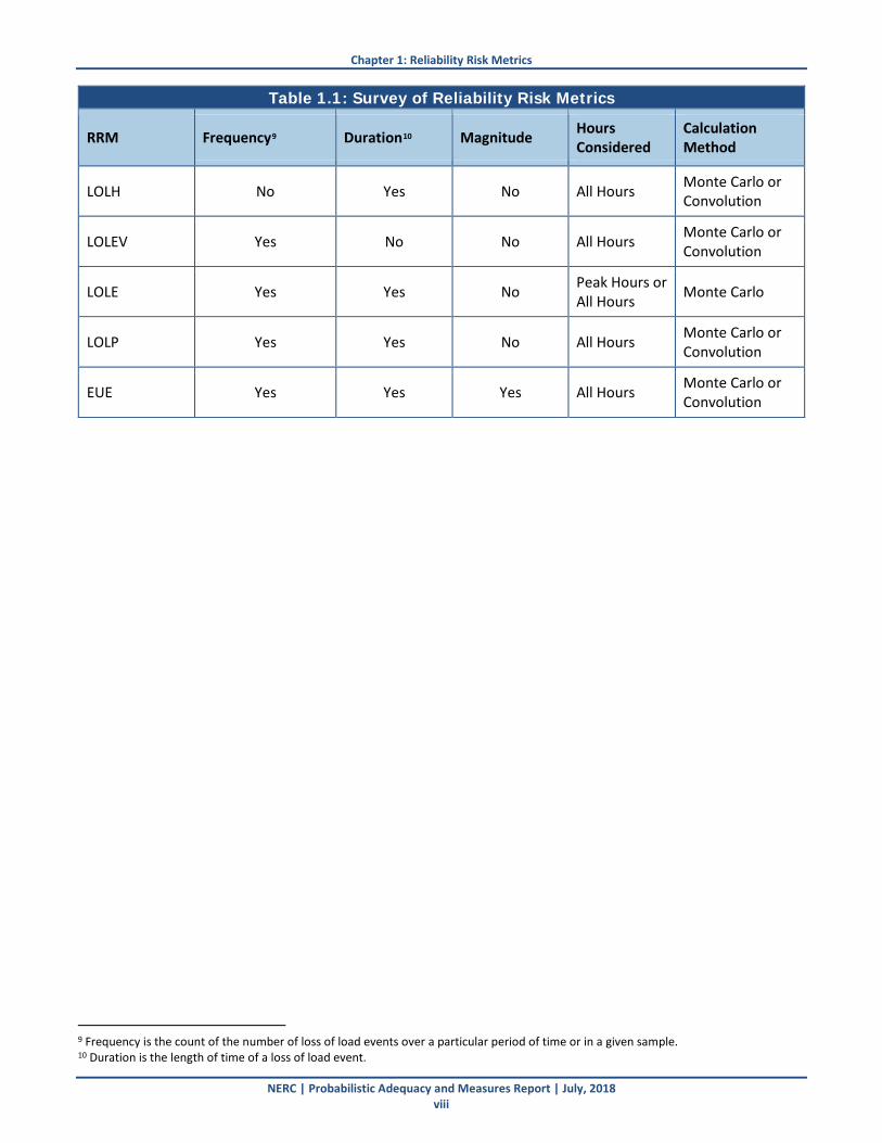
Where 𝐿𝐿𝐷𝐷𝐷𝐷𝑘𝑘 is Energy Not Supplied in 𝑘𝑘th iteration, and N is the total number of iterations. Considerations and Recommendations on the Use of EUE EUE is the only metric that considers magnitude of loss of load events. With the changing generation mix, to make EUE a more effective metric, hourly EUE should be reported for every month or year (24 data points). Summary of Reliability Risk Metrics System needs can be described using three characteristics: frequency, duration, and magnitude. As shown in the summary Table 1.1, each RRM allows planners to identify one or multiple of these characteristics.
Chapter 1: Reliability Risk Metrics
NERC | Probabilistic Adequacy and Measures Report | July, 2018 viii
Table 1.1: Survey of Reliability Risk Metrics
RRM Frequency9 Duration10 Magnitude Hours Considered
Calculation Method
LOLH No Yes No All Hours Monte Carlo or Convolution
LOLEV Yes No No All Hours Monte Carlo or Convolution
LOLE Yes Yes No Peak Hours or All Hours Monte Carlo
LOLP Yes Yes No All Hours Monte Carlo or Convolution
EUE Yes Yes Yes All Hours Monte Carlo or Convolution
9 Frequency is the count of the number of loss of load events over a particular period of time or in a given sample. 10 Duration is the length of time of a loss of load event.

NERC | Probabilistic Adequacy and Measures Report| July, 2018 9
Chapter 2: Applications Although common reliability metrics such as LOLE, LOLP, and LOLEV have been used extensively for a long time, they are not metrics used in the NERC Core Probabilistic Assessment to avoid potential conflicts with regional practices based on different methods. How members of industry define and apply these reliability metrics may vary. This section sheds some light on metrics applications by the industry at large to find commonality and consistencies throughout RRM based on results from an industry survey. Survey results on the use of RRMs are shown in Figure 2.1. LOLP LOLP can be used to determine the probability or likelihood of events due to insufficient capacity. LOLP can be compared across studies and areas as the probability of occurrence in between 0 and 1, producing results on a common spectrum. EUE Among survey responses, 20 of them calculate EUE in their probabilistic studies. EUE is widely used not only in probabilistic studies but also in other planning studies since it is an important indicator of system adequacy and easy to calculate. EUE is very useful in estimating the size of loss of load events so the planners can estimate the cost and impact of the loss of load events. EUE can be used as the basis for reference reserve margin to determine capacity credits for VERs. In addition, EUE can be used to quantify the impacts of extreme weather, common mode failure, etc. LOLH As demonstrated by the results of the attached survey, the LOLH metric is computed by a large number of entities in North America. However, only one entity uses this metric as a reliability criterion, with their criterion set at 2.4 hours per year. Outside of North America, this metric appears to be more widely used as a reliability criterion, particularly in Western Europe, with criteria ranging from three to eight hours per year. LOLE The majority of entities conducting LOLE studies primarily use it to establish resource adequacy criteria. Criteria development entities may also leverage other metrics and factors in their criteria development to determine a sufficient reserve margin to maintain an adequate level of system reliability. LOLE generally helps inform integrated resource planning, market-based resource procurement, generator interconnection queue projects, and other planning activities. Some system planners may also choose to optimize their resource adequacy criteria based on other factors than LOLE, such as, but not limited to, EUE, system and societal costs, and the risk averseness of their regulating bodies and end-use customers. Consider the analogy of an individual’s determination of the appropriate driving speed: the criteria to travel down the highway. The miles per hour (mph) metric is inversely analogous to LOLE (measured at any given point in time) while the speed limit is one criteria (similar to the industry standard 0.1 days per year
Figure 2.1: Survey-Based Results on the Use of Reliability Risk Metrics

Chapter 2: Applications
NERC | Probabilistic Adequacy and Measures Report | July, 2018 x
LOLE) that influences the driver’s ultimate decision to align mph to an optimal driving speed. The driver may choose to drive to the posted speed limit or may choose to optimize based on other factors such as car performance and the driving patterns of others on the highway. The drivers’ (system planners’) criterions may vary given the highways (systems) they are operating on. LOLEV The LOLEV metric is useful in systems that are concerned with the frequency of events, regardless of duration or magnitude. It is also useful for systems where events may occur multiple times in a single day, such as systems with a high load factor, indicating a flatter load shape (e.g. systems with predominately industrial load), or where the system is sensitive to forced outages from larger generators; in such cases, the LOLEV metric may better estimate system risk than the traditional LOLE metric. Some jurisdictions do not differentiate between LOLEV and LOLE; in these cases, the resource adequacy standard is defined as, “one expected event per ten years.” Systems using this standard should be aware that this may lead to a higher level of reliability than applying the standard using the LOLE metric; in these cases, the metric is used to determine resource adequacy requirements for capacity planning purposes or for determining the planning reserve margin.

NERC | Probabilistic Adequacy and Measures Report| July, 2018 11
Chapter 3: Probabilistic Studies Assessing Emerging Reliability Issues The resource mix and its delivery are transforming from large, remotely-located coal and nuclear-fired power plants towards natural gas-fired, renewable energy limited, and DERs. These changes in the generation resource mix and the integration of new technologies are altering the operational characteristics of the grid and will challenge system planners and operators to maintain reliability. Failure to take into account these characteristics and capabilities can lead to insufficient capacity, energy, and ERSs, sometimes called ancillary services, to meet customer demands. The focus of this section is three-fold: first, it surveys the electricity sector existing and future use of probabilistic studies to investigate BPS risks to reliability; second, it tracks evolving emerging trends; and third, it identifies applications for the electricity sector to use known reliability metrics to assess emerging issues. The Use of Probabilistic Studies to Assess Emerging Issues Several emerging key issues have the potential to increase risks to reliability that may require mitigation to maintain BPS reliability. These issues include the following:
• Resource adequacy
• Single-fuel dependency
• Nuclear uncertainty
• Essential reliability services
• DERs
• VER impact on reliability
• Fuel security
• Unit outages (nuclear generation curtailments)
• Transmission aging
• Transmission outages
Previous NERC assessments showed the need to support probability-based resource adequacy assessment due to changing resource mix with significant increases in energy-limited resources, changes in off-peak demand, and other factors can have an effect on resource adequacy.11 As a result, NERC is incorporating more probabilistic approaches into its assessments, including the development of this report. The NERC PAWG examined the use of probabilistic studies in assessing emerging reliability issues; therefore, NERC asked the Regions and other members of the industry what emerging issues or probabilistic studies to investigate. Table 3.1 summarizes survey responses on key emerging reliability issues that probabilistic studies can be used to assess. Survey responses on emerging issues echoed NERC’s key risk profiles and reliability priorities in areas of recommendations where further study, enhanced practices, and ongoing coordination with the industry are needed to ensure reliability.12
11 2016 LTRA Assessment 12 ERO Reliability Risk Priorities Report, 2016

Chapter 3: Probabilistic Studies Assessing Emerging Reliability Issues
NERC | Probabilistic Adequacy and Measures Report | July, 2018 xii
Table 3.1: Probabilistic Studies to Support Addressing Emerging Reliability Issues
Emerging Issue Details
Generation Mix Changes
• Risks outside of peak hours (off season)
• Normal/extreme weather events
• Seasonality
• Replacement/Retirement
• Inertia
Integration of Variable Energy Resources
• Capacity Credit
• Resource Adequacy/Margin (installed capacity requirements/planning reserve margin)
• Ramping/Flexibility/Regulation
Ancillary services
• Pricing/Congestion
• Tie line resource assessments
New Technologies
• Such as Energy Storage (Batteries), Electric Vehicles, Demand Response
• Distributed Resources
• Capacity Credit
Common Mode Failure
• Fuel Security/gas curtailment
• Single Points of Disruption
Transmission planning
• Congestion
• Stability studies
• Dynamic studies
Table 3.2 shows issues that can be addressed using probabilistic analysis and metrics that are not discussed in this report. PAWG recommends that NERC delegates these issues to appropriate committees and working groups.

Chapter 3: Probabilistic Studies Assessing Emerging Reliability Issues
NERC | Probabilistic Adequacy and Measures Report | July, 2018 xiii
Table 3.2: Probabilistic Studies to Support Addressing Emerging Reliability Issues
Emerging Issue Details
Operational Concerns
• Unit commitment
• Over-generation
• Dispatchability
Essential Reliability Services
• Capacity Credit
• Ramping
• Flexibility
• Regulation
Asset Evaluation • Potential resource upgrades, viable replacement resources
Industry Application of Reliability Metrics into Emerging Issues This section focuses on applications by the electricity sector of reliability metrics into emerging issues. Loss of Load Probability No respondents to the industry survey were contemplating moving from a reliability criterion based on an annual metric (LOLE) to a reliability criterion based on LOLH. Generally, LOLH is a more suitable metric in systems with known energy limitations, such as systems with high levels of hydro power generation. Additionally, with the growing penetration of variable energy resources in comparison to traditional base load resources, either as load reducers or as supply, it is anticipated that hourly variations in load and supply will become less predictable. Time series models, which more accurately predict the behavior of stochastic processes such as the variations in wind speed and solar variations, may become more prevalent in probabilistic assessments. This change in modeling may in turn result in a metric such as LOLH, which captures hourly variations in system conditions, becoming increasingly meaningful in measuring the reliability of the system. Expected Unserved Energy EUE along with value of loss load can be used to monetize the cost of loss of load to justify, prioritize, or rank transmission or other capital projects. EUE can be used as a basis for reference reserve margin to determine capacity credits for variable energy resources. In addition, EUE can be used to quantify the impacts of extreme weather, common mode failure, etc. Loss of Load Expectations None of the respondents to the survey suggested use of LOLE for other purposes than to establish resource adequacy criteria. Most of the emerging issues surrounding a changing resource mix need answers to questions regarding energy loss, loss of load duration and frequency, as well as shifts in hourly LOLP from the historical peak time periods. Loss of Load Expected Events The LOLEV metric can be applied to several emerging issues; with respect to generation mix changes, it is excellent metric for addressing risks outside of daily peak hours or shoulder seasons. It can also provide beneficial for integration studies of variable energy resources as it addresses that VERs can provide capacity value outside of

Chapter 3: Probabilistic Studies Assessing Emerging Reliability Issues
NERC | Probabilistic Adequacy and Measures Report | July, 2018 xiv
daily peak hours. As the amount and percentage of distributed resources grow on systems, the LOLEV metric can be used for identifying adequacy shortfalls outside of the daily peak or frequency of loss of load events due to changing load shapes and shifting demands. Loss of Load Hours LOLH provides insight to the impact of energy limited resources on a system’s reliability, particularly in systems with growing penetration of such resources.
NERC | Probabilistic Adequacy and Measures Report| July, 2018 15
Conclusions The NERC Probabilistic Assessment Working Group developed this technical reference report to identify, define, and evaluate probabilistic metrics used in the industry to advance the work of the NERC Probabilistic Assessment Improvement Plan Report and Technical Guidelines Report. Significant changes in the resource mix, including the growing penetration of variable and behind-the-meter generation, have influenced changes on load profiles and have challenged reliability planners’ traditional methods of gauging adequate levels of supply for the BPS. These changes have increased the need to review these traditional, deterministic, and probabilistic approaches to measuring resource adequacy. As a result, NERC has analyzed these probabilistic approaches and created recommendations to meet these needs to assure adequate reserve margins are met and maintain reliability. This technical reference report explored the approaches and applications of commonly used RRMs. It was found that each RRM can measure different aspects of a system’s reliability, such as frequency, duration, and magnitude of loss of load, depending on how the metric is defined and applied. In addition, NERC analyzed commonalities and trends from industry on the application these probabilistic reliability metrics. Results indicated that there is a degree of variability on how similar metrics are defined and applied in gauging resource adequacy across the industry. Recommendations for changes to the application of RRMs were analyzed and discussed to improve their effectiveness. In the face of changes affecting the PBS, NERC will continue to review and provide guidance on the development of probabilistic methods for assuring resource adequacy and reliability. These measures will allow better risk-informed recommendations by planners for policy makers in the face of increasing unpredictability and uncertainty of supply and demands, on the BPS.
NERC | Probabilistic Adequacy and Measures Report| July, 2018 16
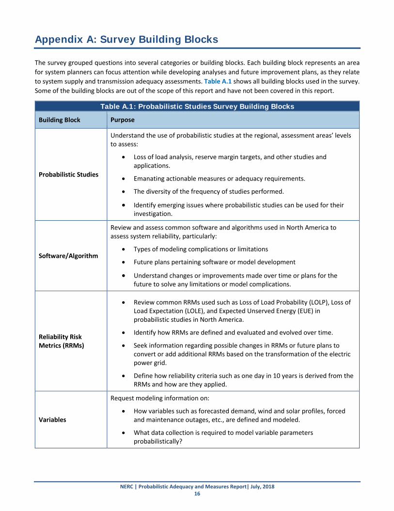
Appendix A: Survey Building Blocks The survey grouped questions into several categories or building blocks. Each building block represents an area for system planners can focus attention while developing analyses and future improvement plans, as they relate to system supply and transmission adequacy assessments. Table A.1 shows all building blocks used in the survey. Some of the building blocks are out of the scope of this report and have not been covered in this report.
Table A.1: Probabilistic Studies Survey Building Blocks
Building Block Purpose
Probabilistic Studies
Understand the use of probabilistic studies at the regional, assessment areas’ levels to assess:
• Loss of load analysis, reserve margin targets, and other studies and applications.
• Emanating actionable measures or adequacy requirements.
• The diversity of the frequency of studies performed.
• Identify emerging issues where probabilistic studies can be used for their investigation.
Software/Algorithm
Review and assess common software and algorithms used in North America to assess system reliability, particularly:
• Types of modeling complications or limitations
• Future plans pertaining software or model development
• Understand changes or improvements made over time or plans for the future to solve any limitations or model complications.
Reliability Risk Metrics (RRMs)
• Review common RRMs used such as Loss of Load Probability (LOLP), Loss of Load Expectation (LOLE), and Expected Unserved Energy (EUE) in probabilistic studies in North America.
• Identify how RRMs are defined and evaluated and evolved over time.
• Seek information regarding possible changes in RRMs or future plans to convert or add additional RRMs based on the transformation of the electric power grid.
• Define how reliability criteria such as one day in 10 years is derived from the RRMs and how are they applied.
Variables
Request modeling information on:
• How variables such as forecasted demand, wind and solar profiles, forced and maintenance outages, etc., are defined and modeled.
• What data collection is required to model variable parameters probabilistically?
Appendix A: Survey Building Blocks
NERC | Probabilistic Adequacy and Measures Report | July, 2018 xvii
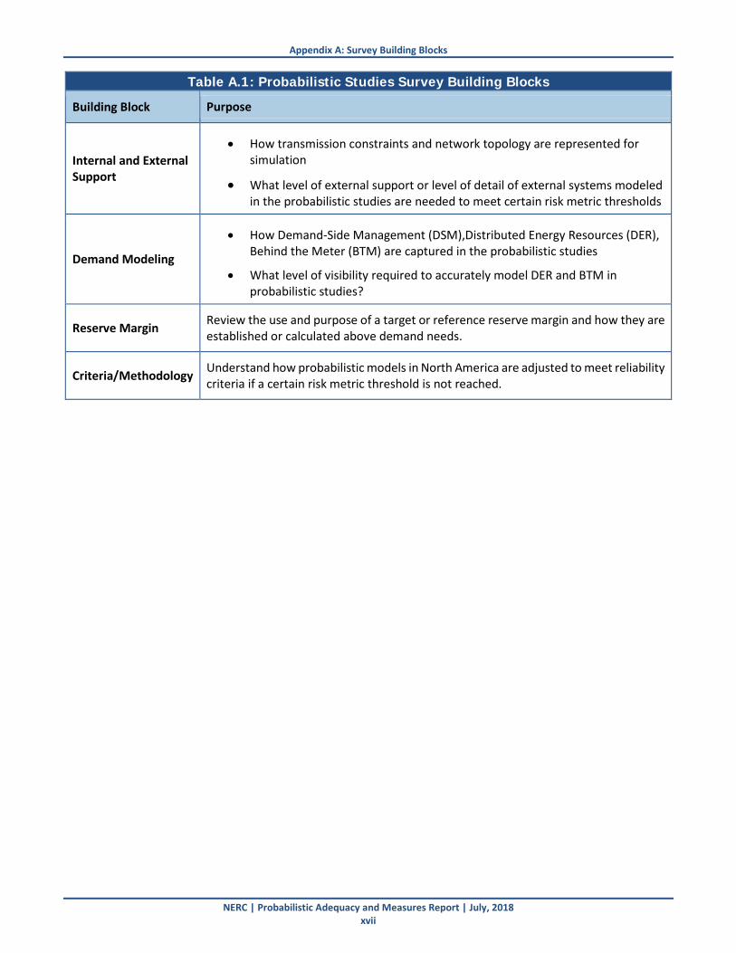
Table A.1: Probabilistic Studies Survey Building Blocks
Building Block Purpose
Internal and External Support
• How transmission constraints and network topology are represented for simulation
• What level of external support or level of detail of external systems modeled in the probabilistic studies are needed to meet certain risk metric thresholds
Demand Modeling
• How Demand-Side Management (DSM),Distributed Energy Resources (DER), Behind the Meter (BTM) are captured in the probabilistic studies
• What level of visibility required to accurately model DER and BTM in probabilistic studies?
Reserve Margin Review the use and purpose of a target or reference reserve margin and how they are established or calculated above demand needs.
Criteria/Methodology Understand how probabilistic models in North America are adjusted to meet reliability criteria if a certain risk metric threshold is not reached.

NERC | Probabilistic Adequacy and Measures Report| July, 2018 18
Appendix B: Survey Questions 1. Enter the requested information below.
Region or Utility Name:
Survey Respondent(s):
Email and Phone Number:
Date Survey Completed: 2. What do you use probabilistic studies for? Explanation: At the regional levels probabilistic studies are used for loss of load analysis while others use them for reference margin setting, etc.…
Planning Reserve Margin Loss of Load Expectation Ramping Capabilities Effective Load Caring Capabilities Transmission Planning Studies Other (Please specify in your response)
Comments: 3. What actionable information emanates from this analysis? What information and how it is used? Explanation: Results from the studies can sometimes feed into actionable measures or requirements.
4. What is the frequency of the probabilistic studies? Why? Explanation: Studies performed annually, seasonally, monthly, etc.…
5. What emerging issues do you use or may use probabilistic studies to investigate? Explanation: Emerging issues such as variable resource integration, flexible resource capabilities, etc.…
6. What software is used? Explanation: Examples like GE-MARS, SERVM, etc...
7. What solving algorithm is used? Explanation: Examples like Monte Carlo, Convolution, etc...
8. Modeling complications? Explanation: Any limitations or complications you have run into when trying to perform the studies.

Appendix B: Survey Questions
NERC | Probabilistic Adequacy and Measures Report | July, 2018 xix
Examples like software limitations, renewable modeling time series vs. ELCC, interconnected vs islanded systems, computational runtime, market parameters, etc.…
9. Changes over time? Explanation: Have you been able to resolve the complications, if so how?
10. Future plans to change/add more software tools? Explanation: Any future plans pertaining to software development or model changes.
11. What metrics are you using? Explanation: What metrics are you studying in your probabilistic studies? Examples are Loss-Of-Load Probability (LOLP), Loss-Of-Load Expectation (LOLE), Expected Unserved Energy (EUE), etc.…
Loss-of-Load Probability (LOLP) Expected Unserved Energy (EUE) Loss-of-Load Hours (LOLH) Loss-of-Load Expectation (LOLE) Loss-of-Load Events (LOLEV) Other (please specify)
12. How are the metrics defined? Explanation: Formulas to calculate the metrics, or what the criteria mean to you.
13. Are the metrics based on certain hours of the day? Such as peak hours vs. all hours? Explanation: Sometimes metrics are only applied to the daily peak hour sometimes to all hours.
14. What horizon is being used (weekly, monthly, seasonal, and annual)? Explanation: Are the metrics calculated for different time periods like an overall annual risk metric or weekly risk metrics?
15. Do different time horizons/seasons drive the use of different metrics? Explanation: Do you find the need to study different metrics depending on what period is being studied?
16. Any plans to change and/or add risk metrics? Explanation: Any future plans to convert to other metrics and why?

Appendix B: Survey Questions
NERC | Probabilistic Adequacy and Measures Report | July, 2018 xx
17. Have the metrics changed over time and why changes were made? Explanation: How have the metrics studied evolved over the years?
18. Do you evaluate reliability costs as part of your probabilistic studies? Explanation: Some areas assess the economics of reducing risk metric values. For example, this can be accomplished by accounting for incremental resource capital/production costs, Value of Lost Load (VOLL), and costs.
19. What criteria is derived from the metrics? And how are they applied? Explanation: For example a 1 day in 10 criteria is derived from LOLE metric.
20. What variables are modeled stochastically, and parameters varied for scenario analysis? Explanation: i.e., Demand, Load Forecast Uncertainty, Generator Unplanned Outages, Transmission Unplanned Outages, Variable Resource Generation, etc.
21. How are the variables identified in question 20 modeled? Explanation: Some areas use probabilistic distributions around an expected forecast and then randomly sample from these distributions.
22. What data is being used to model the variables identified in question 20? Explanation: For example, what renewable data you collect to model your variable resources? GADS data used for planned outages and maintenance.
23. Are internal transmission constraints modeled? Explanation: Internal transmission constraints could be modeled in probabilistic studies by using a transportation model logic or a multi-area reliability model to assess the transmission import or export constraints that would impact system or sub-area risk metrics.
24. How are transmission constraints and network topology represented for simulation? Explanation: Examples are Nodal (all topology is modeled to the bus-level) or Zonal (All major constraints are modeled in a "Bubble & Pipe" representation
25. Is external support or demand modeled in the probabilistic studies? Explanation: Are other areas connected to your system that might impact system or sub-area risk metrics through transmission import or export needs.

Appendix B: Survey Questions
NERC | Probabilistic Adequacy and Measures Report | July, 2018 xxi
26. How much external support is relied upon in the probabilistic studies? Explanation: Is there constant imports needed to meet certain risk metric thresholds?
27. Does your probabilistic studies capture Demand-Side Management (DSM)? If so, describe how that is accomplished. Explanation: DR programs which are dispatchable can be modeled as energy limited resources with values for capacity and energy. EE programs which are typically non-dispatch able can be modeled as non-dispatch able resources with values for capacity and an hourly impact profile or shape.
28. Does your probabilistic studies capture Distributed Energy Resources (DER) or Behind-The-Meter (BTM) generation? If so, describe how that is accomplished. Explanation: DR programs which are dispatchable can be modeled as energy limited resources with values for capacity and energy. EE programs which are typically non-dispatch able can be modeled as non-dispatch able resources with values for capacity and an hourly impact profile or shape.
29. If so, what level of BTM or DER visibility do you have to model such variables? Explanation: Is there a way that you capture what may or may not have been contributed to the system by these types of variables?
30. Do you establish a target or reference reserve margin? Explanation: Amount of capacity above demand needs for reserve purposes.
31. If so, how is the target or reference reserve margin calculated and how is the reserve margin applied to the assessment area? Explanation: Some areas set a reference reserve margin based on a Loss-Of-Load Expectation (LOLE) of 1-day-in-10 criteria.
32. What is the purpose of setting the reference reserve margin? Explanation: Is it set for compliance reasons, state & provincial requirements, or best practices.
33. For your modeling, how do you adjust your system to meet reliability criteria if a certain risk metric threshold is not reached? Explanation: Examples would be adjust load or adjust resources.

Appendix B: Survey Questions
NERC | Probabilistic Adequacy and Measures Report | July, 2018 xxii
34. What other types of data/details not discussed above are included in your probabilistic modeling? Explanation: Anything not discussed above that you believe is important to note in your probabilistic studies? (Without going into specific details on modeling or results).
NERC | Probabilistic Adequacy and Measures Report| July, 2018 23
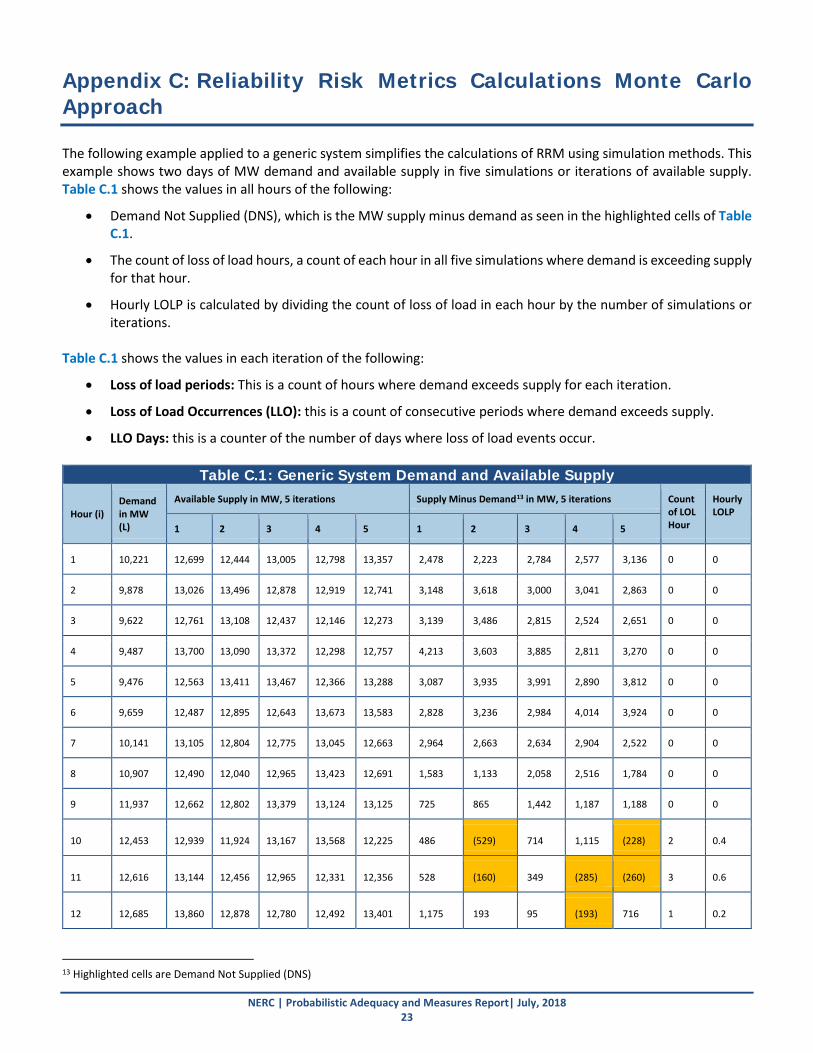
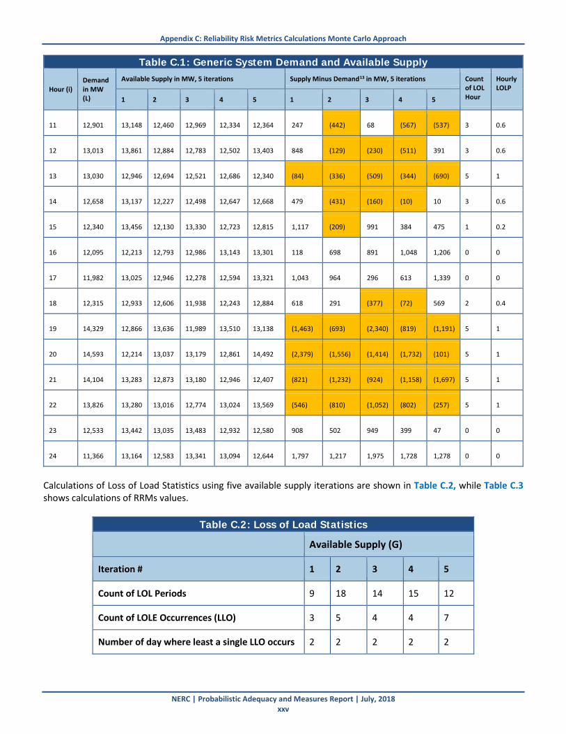
Appendix C: Reliability Risk Metrics Calculations Monte Carlo Approach The following example applied to a generic system simplifies the calculations of RRM using simulation methods. This example shows two days of MW demand and available supply in five simulations or iterations of available supply. Table C.1 shows the values in all hours of the following:
• Demand Not Supplied (DNS), which is the MW supply minus demand as seen in the highlighted cells of Table C.1.
• The count of loss of load hours, a count of each hour in all five simulations where demand is exceeding supply for that hour.
• Hourly LOLP is calculated by dividing the count of loss of load in each hour by the number of simulations or iterations.
Table C.1 shows the values in each iteration of the following:
• Loss of load periods: This is a count of hours where demand exceeds supply for each iteration.
• Loss of Load Occurrences (LLO): this is a count of consecutive periods where demand exceeds supply.
• LLO Days: this is a counter of the number of days where loss of load events occur.
Table C.1: Generic System Demand and Available Supply
Hour (i) Demand in MW (L)
Available Supply in MW, 5 iterations Supply Minus Demand13 in MW, 5 iterations Count of LOL Hour
Hourly LOLP
1 2 3 4 5 1 2 3 4 5
1 10,221 12,699 12,444 13,005 12,798 13,357 2,478 2,223 2,784 2,577 3,136 0 0
2 9,878 13,026 13,496 12,878 12,919 12,741 3,148 3,618 3,000 3,041 2,863 0 0
3 9,622 12,761 13,108 12,437 12,146 12,273 3,139 3,486 2,815 2,524 2,651 0 0
4 9,487 13,700 13,090 13,372 12,298 12,757 4,213 3,603 3,885 2,811 3,270 0 0
5 9,476 12,563 13,411 13,467 12,366 13,288 3,087 3,935 3,991 2,890 3,812 0 0
6 9,659 12,487 12,895 12,643 13,673 13,583 2,828 3,236 2,984 4,014 3,924 0 0
7 10,141 13,105 12,804 12,775 13,045 12,663 2,964 2,663 2,634 2,904 2,522 0 0
8 10,907 12,490 12,040 12,965 13,423 12,691 1,583 1,133 2,058 2,516 1,784 0 0
9 11,937 12,662 12,802 13,379 13,124 13,125 725 865 1,442 1,187 1,188 0 0
10 12,453 12,939 11,924 13,167 13,568 12,225 486 (529) 714 1,115 (228) 2 0.4
11 12,616 13,144 12,456 12,965 12,331 12,356 528 (160) 349 (285) (260) 3 0.6
12 12,685 13,860 12,878 12,780 12,492 13,401 1,175 193 95 (193) 716 1 0.2
13 Highlighted cells are Demand Not Supplied (DNS)
Appendix C: Reliability Risk Metrics Calculations Monte Carlo Approach
NERC | Probabilistic Adequacy and Measures Report | July, 2018 xxiv
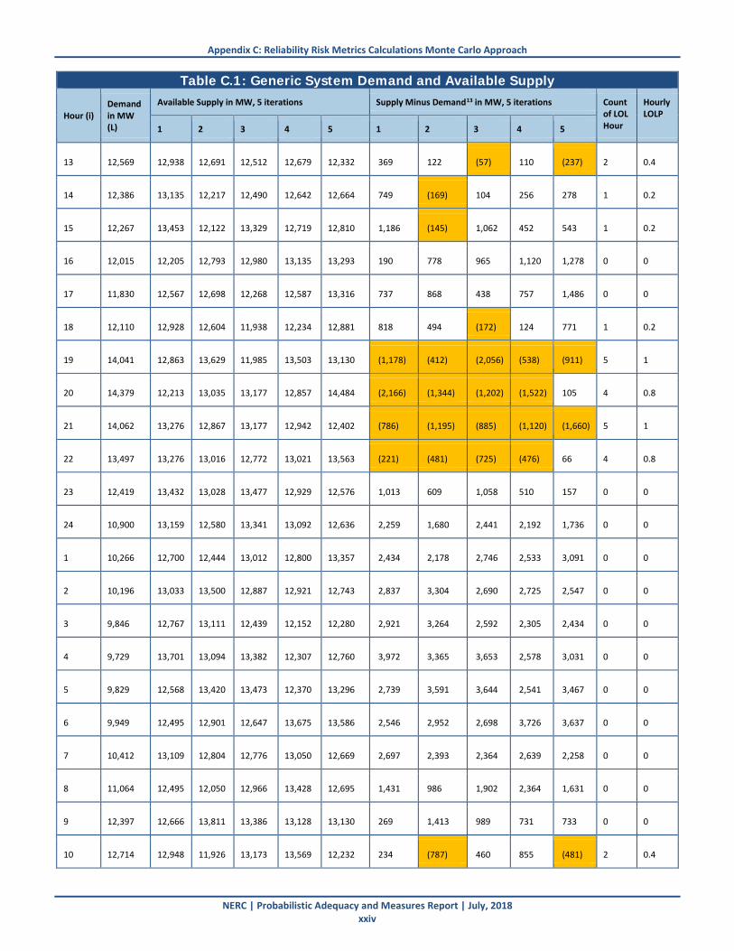
Table C.1: Generic System Demand and Available Supply
Hour (i) Demand in MW (L)
Available Supply in MW, 5 iterations Supply Minus Demand13 in MW, 5 iterations Count of LOL Hour
Hourly LOLP
1 2 3 4 5 1 2 3 4 5
13 12,569 12,938 12,691 12,512 12,679 12,332 369 122 (57) 110 (237) 2 0.4
14 12,386 13,135 12,217 12,490 12,642 12,664 749 (169) 104 256 278 1 0.2
15 12,267 13,453 12,122 13,329 12,719 12,810 1,186 (145) 1,062 452 543 1 0.2
16 12,015 12,205 12,793 12,980 13,135 13,293 190 778 965 1,120 1,278 0 0
17 11,830 12,567 12,698 12,268 12,587 13,316 737 868 438 757 1,486 0 0
18 12,110 12,928 12,604 11,938 12,234 12,881 818 494 (172) 124 771 1 0.2
19 14,041 12,863 13,629 11,985 13,503 13,130 (1,178) (412) (2,056) (538) (911) 5 1
20 14,379 12,213 13,035 13,177 12,857 14,484 (2,166) (1,344) (1,202) (1,522) 105 4 0.8
21 14,062 13,276 12,867 13,177 12,942 12,402 (786) (1,195) (885) (1,120) (1,660) 5 1
22 13,497 13,276 13,016 12,772 13,021 13,563 (221) (481) (725) (476) 66 4 0.8
23 12,419 13,432 13,028 13,477 12,929 12,576 1,013 609 1,058 510 157 0 0
24 10,900 13,159 12,580 13,341 13,092 12,636 2,259 1,680 2,441 2,192 1,736 0 0
1 10,266 12,700 12,444 13,012 12,800 13,357 2,434 2,178 2,746 2,533 3,091 0 0
2 10,196 13,033 13,500 12,887 12,921 12,743 2,837 3,304 2,690 2,725 2,547 0 0
3 9,846 12,767 13,111 12,439 12,152 12,280 2,921 3,264 2,592 2,305 2,434 0 0
4 9,729 13,701 13,094 13,382 12,307 12,760 3,972 3,365 3,653 2,578 3,031 0 0
5 9,829 12,568 13,420 13,473 12,370 13,296 2,739 3,591 3,644 2,541 3,467 0 0
6 9,949 12,495 12,901 12,647 13,675 13,586 2,546 2,952 2,698 3,726 3,637 0 0
7 10,412 13,109 12,804 12,776 13,050 12,669 2,697 2,393 2,364 2,639 2,258 0 0
8 11,064 12,495 12,050 12,966 13,428 12,695 1,431 986 1,902 2,364 1,631 0 0
9 12,397 12,666 13,811 13,386 13,128 13,130 269 1,413 989 731 733 0 0
10 12,714 12,948 11,926 13,173 13,569 12,232 234 (787) 460 855 (481) 2 0.4
Appendix C: Reliability Risk Metrics Calculations Monte Carlo Approach
NERC | Probabilistic Adequacy and Measures Report | July, 2018 xxv
Table C.1: Generic System Demand and Available Supply
Hour (i) Demand in MW (L)
Available Supply in MW, 5 iterations Supply Minus Demand13 in MW, 5 iterations Count of LOL Hour
Hourly LOLP
1 2 3 4 5 1 2 3 4 5
11 12,901 13,148 12,460 12,969 12,334 12,364 247 (442) 68 (567) (537) 3 0.6
12 13,013 13,861 12,884 12,783 12,502 13,403 848 (129) (230) (511) 391 3 0.6
13 13,030 12,946 12,694 12,521 12,686 12,340 (84) (336) (509) (344) (690) 5 1
14 12,658 13,137 12,227 12,498 12,647 12,668 479 (431) (160) (10) 10 3 0.6
15 12,340 13,456 12,130 13,330 12,723 12,815 1,117 (209) 991 384 475 1 0.2
16 12,095 12,213 12,793 12,986 13,143 13,301 118 698 891 1,048 1,206 0 0
17 11,982 13,025 12,946 12,278 12,594 13,321 1,043 964 296 613 1,339 0 0
18 12,315 12,933 12,606 11,938 12,243 12,884 618 291 (377) (72) 569 2 0.4
19 14,329 12,866 13,636 11,989 13,510 13,138 (1,463) (693) (2,340) (819) (1,191) 5 1
20 14,593 12,214 13,037 13,179 12,861 14,492 (2,379) (1,556) (1,414) (1,732) (101) 5 1
21 14,104 13,283 12,873 13,180 12,946 12,407 (821) (1,232) (924) (1,158) (1,697) 5 1
22 13,826 13,280 13,016 12,774 13,024 13,569 (546) (810) (1,052) (802) (257) 5 1
23 12,533 13,442 13,035 13,483 12,932 12,580 908 502 949 399 47 0 0
24 11,366 13,164 12,583 13,341 13,094 12,644 1,797 1,217 1,975 1,728 1,278 0 0
Calculations of Loss of Load Statistics using five available supply iterations are shown in Table C.2, while Table C.3 shows calculations of RRMs values.
Table C.2: Loss of Load Statistics
Available Supply (G)
Iteration # 1 2 3 4 5
Count of LOL Periods 9 18 14 15 12
Count of LOLE Occurrences (LLO) 3 5 4 4 7
Number of day where least a single LLO occurs 2 2 2 2 2
Appendix C: Reliability Risk Metrics Calculations Monte Carlo Approach
NERC | Probabilistic Adequacy and Measures Report | July, 2018 xxvi
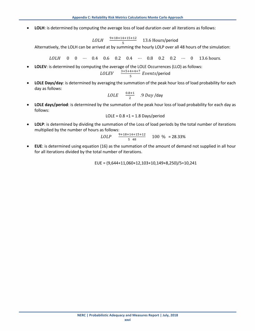
• LOLH: is determined by computing the average loss of load duration over all iterations as follows:
𝐿𝐿𝐿𝐿𝐿𝐿𝐿𝐿 = 9+18+14+15+125
= 13.6 Hours/period Alternatively, the LOLH can be arrived at by summing the hourly LOLP over all 48 hours of the simulation:
𝐿𝐿𝐿𝐿𝐿𝐿𝐿𝐿 = 0 + 0 + ⋯+ 0.4 + 0.6 + 0.2 + 0.4 + ⋯+ 0.8 + 0.2 + 0.2 + ⋯+ 0 = 13.6 hours.
• LOLEV: is determined by computing the average of the LOLE Occurrences (LLO) as follows: 𝐿𝐿𝐿𝐿𝐿𝐿𝐿𝐿𝐿𝐿 = 3+5+4+4+7
5 𝐿𝐿𝐸𝐸𝐸𝐸𝐸𝐸𝐸𝐸𝐸𝐸/period
• LOLE Days/day: is determined by averaging the summation of the peak hour loss of load probability for each day as follows:
𝐿𝐿𝐿𝐿𝐿𝐿𝐿𝐿 = 0.8+12
= .9 𝐷𝐷𝑚𝑚𝐷𝐷 /day
• LOLE days/period: is determined by the summation of the peak hour loss of load probability for each day as follows:
LOLE = 0.8 +1 = 1.8 Days/period
• LOLP: is determined by dividing the summation of the Loss of load periods by the total number of iterations multiplied by the number of hours as follows:
𝐿𝐿𝐿𝐿𝐿𝐿𝐿𝐿 = 9+18+14+15+125×48
× 100(%) = 28.33%
• EUE: is determined using equation (16) as the summation of the amount of demand not supplied in all hour for all iterations divided by the total number of iterations.
EUE = (9,644+11,060+12,103+10,149+8,250)/5=10,241

Appendix C: Reliability Risk Metrics Calculations Monte Carlo Approach
NERC | Probabilistic Adequacy and Measures Report | July, 2018 xxvii
Table C.3: Calculations of Reliability Risk Metrics (RRM)
RRM Value
LOLH (Hours/period) 13.6
LOLEV (Events/period) 4.60
LOLE (Days/day) LOLE (Days/period)
0.9 1.8
LOLP (%) 28.3
EUE (MWh) 10,241
Figure C.1 shows second iteration supply, demand, and loss of load events in day one and day two. Using iteration two, three loss of load events in day 1 are found whereas two loss of load events in day 2.
Figure C.1: Generic System Loss of Load Events—Iteration 2
NERC | Probabilistic Adequacy and Measures Report| July, 2018 28
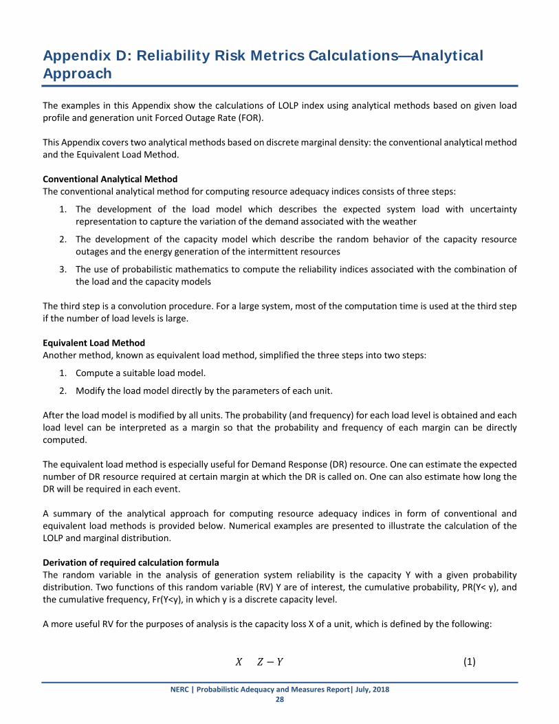
Appendix D: Reliability Risk Metrics Calculations—Analytical Approach The examples in this Appendix show the calculations of LOLP index using analytical methods based on given load profile and generation unit Forced Outage Rate (FOR). This Appendix covers two analytical methods based on discrete marginal density: the conventional analytical method and the Equivalent Load Method. Conventional Analytical Method The conventional analytical method for computing resource adequacy indices consists of three steps:
1. The development of the load model which describes the expected system load with uncertainty representation to capture the variation of the demand associated with the weather
2. The development of the capacity model which describe the random behavior of the capacity resource outages and the energy generation of the intermittent resources
3. The use of probabilistic mathematics to compute the reliability indices associated with the combination of the load and the capacity models
The third step is a convolution procedure. For a large system, most of the computation time is used at the third step if the number of load levels is large. Equivalent Load Method Another method, known as equivalent load method, simplified the three steps into two steps:
1. Compute a suitable load model.
2. Modify the load model directly by the parameters of each unit. After the load model is modified by all units. The probability (and frequency) for each load level is obtained and each load level can be interpreted as a margin so that the probability and frequency of each margin can be directly computed. The equivalent load method is especially useful for Demand Response (DR) resource. One can estimate the expected number of DR resource required at certain margin at which the DR is called on. One can also estimate how long the DR will be required in each event. A summary of the analytical approach for computing resource adequacy indices in form of conventional and equivalent load methods is provided below. Numerical examples are presented to illustrate the calculation of the LOLP and marginal distribution. Derivation of required calculation formula The random variable in the analysis of generation system reliability is the capacity Y with a given probability distribution. Two functions of this random variable (RV) Y are of interest, the cumulative probability, PR(Y< y), and the cumulative frequency, Fr(Y<y), in which y is a discrete capacity level. A more useful RV for the purposes of analysis is the capacity loss X of a unit, which is defined by the following:
𝑋𝑋 = 𝑍𝑍 − 𝑌𝑌 (1)
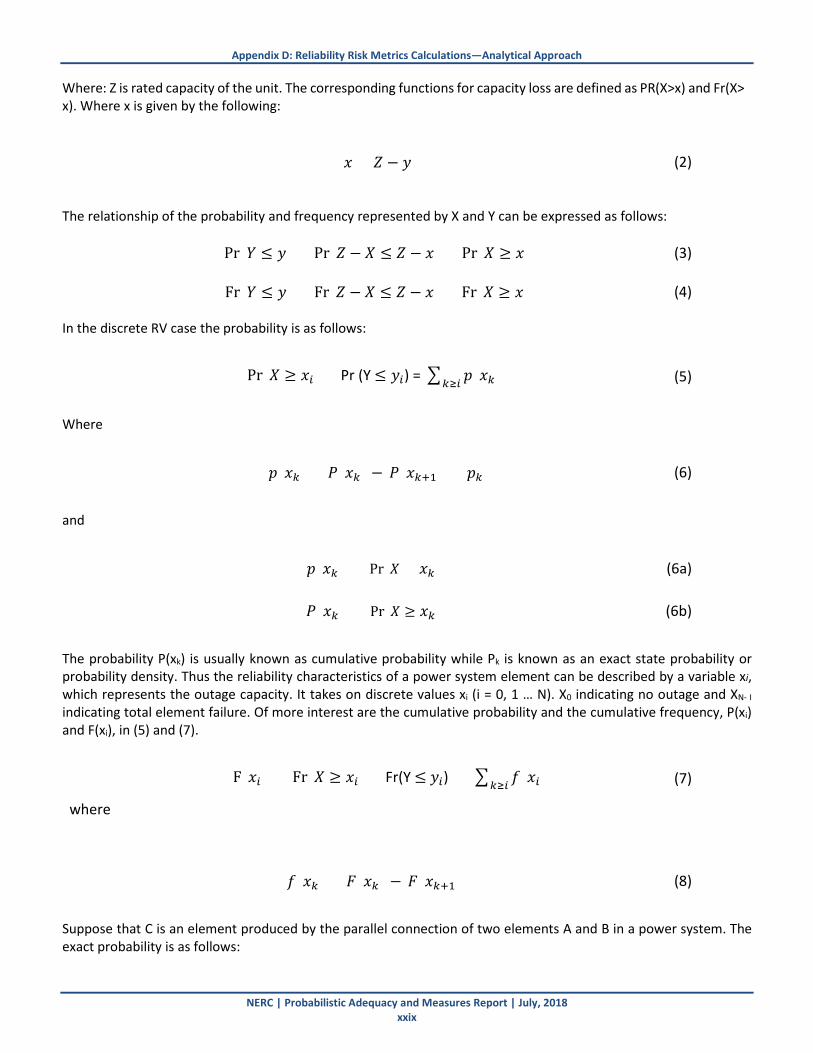
Appendix D: Reliability Risk Metrics Calculations—Analytical Approach
NERC | Probabilistic Adequacy and Measures Report | July, 2018 xxix
Where: Z is rated capacity of the unit. The corresponding functions for capacity loss are defined as PR(X>x) and Fr(X> x). Where x is given by the following:
𝑚𝑚 = 𝑍𝑍 − 𝐷𝐷 (2)
The relationship of the probability and frequency represented by X and Y can be expressed as follows: Pr(𝑌𝑌 ≤ 𝐷𝐷) = Pr(𝑍𝑍 − 𝑋𝑋 ≤ 𝑍𝑍 − 𝑚𝑚) = Pr (𝑋𝑋 ≥ 𝑚𝑚) (3)
Fr(𝑌𝑌 ≤ 𝐷𝐷) = Fr(𝑍𝑍 − 𝑋𝑋 ≤ 𝑍𝑍 − 𝑚𝑚) = Fr (𝑋𝑋 ≥ 𝑚𝑚) (4)
In the discrete RV case the probability is as follows: Pr(𝑋𝑋 ≥ 𝑚𝑚𝑘𝑘) = Pr (Y ≤ 𝐷𝐷𝑘𝑘) = � 𝑝𝑝(𝑚𝑚𝑘𝑘)𝑘𝑘≥𝑘𝑘 (5)
Where
𝑝𝑝(𝑚𝑚𝑘𝑘) = 𝐿𝐿(𝑚𝑚𝑘𝑘) − 𝐿𝐿(𝑚𝑚𝑘𝑘+1 ) = 𝑝𝑝𝑘𝑘 (6)
and
𝑝𝑝(𝑚𝑚𝑘𝑘) = Pr (𝑋𝑋 = 𝑚𝑚𝑘𝑘) (6a)
𝐿𝐿(𝑚𝑚𝑘𝑘) = Pr (𝑋𝑋 ≥ 𝑚𝑚𝑘𝑘) (6b)
The probability P(xk) is usually known as cumulative probability while Pk is known as an exact state probability or probability density. Thus the reliability characteristics of a power system element can be described by a variable xi, which represents the outage capacity. It takes on discrete values xi (i = 0, 1 … N). X0 indicating no outage and XN- I
indicating total element failure. Of more interest are the cumulative probability and the cumulative frequency, P(xi) and F(xi), in (5) and (7). F(𝑚𝑚𝑘𝑘) = Fr(𝑋𝑋 ≥ 𝑚𝑚𝑘𝑘) = Fr(Y ≤ 𝐷𝐷𝑘𝑘) = � 𝑖𝑖(𝑚𝑚𝑘𝑘)𝑘𝑘≥𝑘𝑘 (7)
where
𝑖𝑖(𝑚𝑚𝑘𝑘) = 𝐹𝐹(𝑚𝑚𝑘𝑘) − 𝐹𝐹(𝑚𝑚𝑘𝑘+1 ) (8)
Suppose that C is an element produced by the parallel connection of two elements A and B in a power system. The exact probability is as follows:
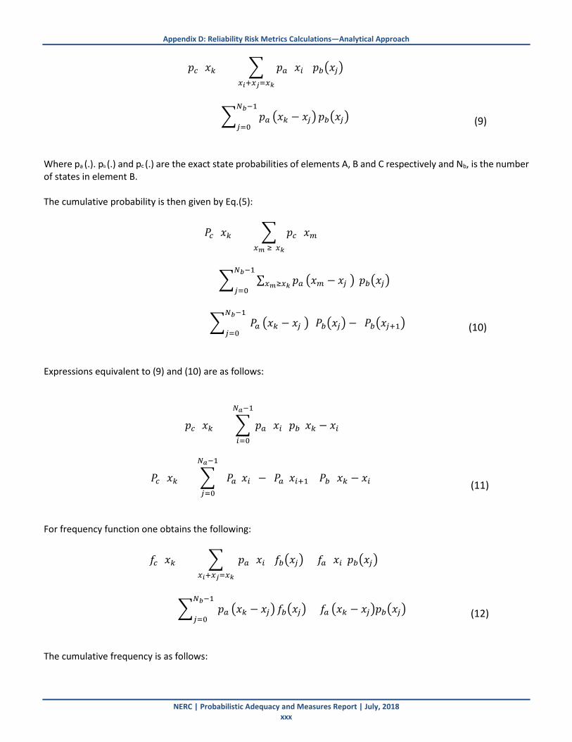
Appendix D: Reliability Risk Metrics Calculations—Analytical Approach
NERC | Probabilistic Adequacy and Measures Report | July, 2018 xxx
𝑝𝑝𝑐𝑐 (𝑚𝑚𝑘𝑘) = � 𝑝𝑝𝑎𝑎 (𝑚𝑚𝑘𝑘)𝑥𝑥𝑖𝑖+𝑥𝑥𝑗𝑗=𝑥𝑥𝑘𝑘
𝑝𝑝𝑏𝑏�𝑚𝑚𝑗𝑗�
= � 𝑝𝑝𝑎𝑎 �𝑚𝑚𝑘𝑘 − 𝑚𝑚𝑗𝑗�𝑁𝑁𝑏𝑏−1
𝑗𝑗=0𝑝𝑝𝑏𝑏�𝑚𝑚𝑗𝑗�
(9)
Where pa (.). pb (.) and pc (.) are the exact state probabilities of elements A, B and C respectively and Nb, is the number of states in element B.
The cumulative probability is then given by Eq.(5):
𝐿𝐿𝑐𝑐 (𝑚𝑚𝑘𝑘) = � 𝑝𝑝𝑐𝑐 (𝑚𝑚𝑚𝑚)
𝑥𝑥𝑚𝑚 ≥ 𝑥𝑥𝑘𝑘
= � ∑ 𝑝𝑝𝑎𝑎 �𝑚𝑚𝑚𝑚 − 𝑚𝑚𝑗𝑗 �𝑥𝑥𝑚𝑚≥𝑥𝑥𝑘𝑘 𝑝𝑝𝑏𝑏�𝑚𝑚𝑗𝑗�𝑁𝑁𝑏𝑏−1
𝑗𝑗=0
= � 𝐿𝐿𝑎𝑎 �𝑚𝑚𝑘𝑘 − 𝑚𝑚𝑗𝑗 � [𝐿𝐿𝑏𝑏�𝑚𝑚𝑗𝑗� − 𝐿𝐿𝑏𝑏�𝑚𝑚𝑗𝑗+1�]𝑁𝑁𝑏𝑏−1
𝑗𝑗=0
(10)
Expressions equivalent to (9) and (10) are as follows:
𝑝𝑝𝑐𝑐 (𝑚𝑚𝑘𝑘) = � 𝑝𝑝𝑎𝑎 (𝑚𝑚𝑘𝑘)𝑁𝑁𝑎𝑎−1
𝑘𝑘=0
𝑝𝑝𝑏𝑏(𝑚𝑚𝑘𝑘 − 𝑚𝑚𝑘𝑘)
𝐿𝐿𝑐𝑐 (𝑚𝑚𝑘𝑘) = � [𝐿𝐿𝑎𝑎(𝑚𝑚𝑘𝑘) − 𝐿𝐿𝑎𝑎(𝑚𝑚𝑘𝑘+1)]𝑁𝑁𝑎𝑎−1
𝑗𝑗=0
𝐿𝐿𝑏𝑏 (𝑚𝑚𝑘𝑘 − 𝑚𝑚𝑘𝑘 )
(11)
For frequency function one obtains the following: 𝑖𝑖𝑐𝑐 (𝑚𝑚𝑘𝑘) = � [𝑝𝑝𝑎𝑎 (𝑚𝑚𝑘𝑘)
𝑥𝑥𝑖𝑖+𝑥𝑥𝑗𝑗=𝑥𝑥𝑘𝑘
𝑖𝑖𝑏𝑏�𝑚𝑚𝑗𝑗� + 𝑖𝑖𝑎𝑎 (𝑚𝑚𝑘𝑘)𝑝𝑝𝑏𝑏�𝑚𝑚𝑗𝑗�]
= � [𝑝𝑝𝑎𝑎 �𝑚𝑚𝑘𝑘 − 𝑚𝑚𝑗𝑗�𝑁𝑁𝑏𝑏−1
𝑗𝑗=0𝑖𝑖𝑏𝑏�𝑚𝑚𝑗𝑗� + 𝑖𝑖𝑎𝑎 �𝑚𝑚𝑘𝑘 − 𝑚𝑚𝑗𝑗�𝑝𝑝𝑏𝑏�𝑚𝑚𝑗𝑗�]
(12)
The cumulative frequency is as follows:
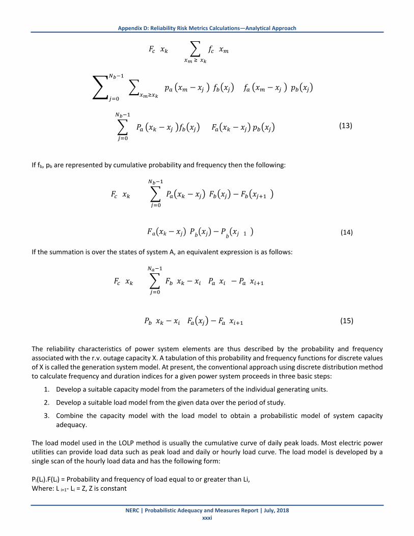
Appendix D: Reliability Risk Metrics Calculations—Analytical Approach
NERC | Probabilistic Adequacy and Measures Report | July, 2018 xxxi
𝐹𝐹𝑐𝑐 (𝑚𝑚𝑘𝑘) = � 𝑖𝑖𝑐𝑐 (𝑚𝑚𝑚𝑚)𝑥𝑥𝑚𝑚 ≥ 𝑥𝑥𝑘𝑘
= � � [𝑝𝑝𝑎𝑎 �𝑚𝑚𝑚𝑚 − 𝑚𝑚𝑗𝑗 �𝑥𝑥𝑚𝑚≥𝑥𝑥𝑘𝑘
𝑖𝑖𝑏𝑏�𝑚𝑚𝑗𝑗� +𝑁𝑁𝑏𝑏−1
𝑗𝑗=0
𝑖𝑖𝑎𝑎 �𝑚𝑚𝑚𝑚 − 𝑚𝑚𝑗𝑗 � 𝑝𝑝𝑏𝑏�𝑚𝑚𝑗𝑗�]
= � [𝐿𝐿𝑎𝑎 �𝑚𝑚𝑘𝑘 − 𝑚𝑚𝑗𝑗 �𝑖𝑖𝑏𝑏�𝑚𝑚𝑗𝑗� + 𝐹𝐹𝑎𝑎�𝑚𝑚𝑘𝑘 − 𝑚𝑚𝑗𝑗� 𝑝𝑝𝑏𝑏�𝑚𝑚𝑗𝑗�]𝑁𝑁𝑏𝑏−1
𝑗𝑗=0
(13)
If fb, pb are represented by cumulative probability and frequency then the following:
𝐹𝐹𝑐𝑐 (𝑚𝑚𝑘𝑘) = � [𝐿𝐿𝑎𝑎�𝑚𝑚𝑘𝑘 − 𝑚𝑚𝑗𝑗�(𝐹𝐹𝑏𝑏�𝑚𝑚𝑗𝑗� − 𝐹𝐹𝑏𝑏�𝑚𝑚𝑗𝑗+1)�
𝑁𝑁𝑏𝑏−1
𝑗𝑗=0
+ 𝐹𝐹𝑚𝑚�𝑚𝑚𝑘𝑘 − 𝑚𝑚𝑗𝑗�(𝐿𝐿𝑏𝑏�𝑚𝑚𝑗𝑗� − 𝐿𝐿𝑏𝑏�𝑚𝑚𝑗𝑗+1)�] (14)
If the summation is over the states of system A, an equivalent expression is as follows:
𝐹𝐹𝑐𝑐 (𝑚𝑚𝑘𝑘) = � [𝐹𝐹𝑏𝑏(𝑚𝑚𝑘𝑘 − 𝑚𝑚𝑘𝑘)(𝐿𝐿𝑎𝑎(𝑚𝑚𝑘𝑘) − 𝐿𝐿𝑎𝑎(𝑚𝑚𝑘𝑘+1))
𝑁𝑁𝑎𝑎−1
𝑗𝑗=0
+𝐿𝐿𝑏𝑏(𝑚𝑚𝑘𝑘 − 𝑚𝑚𝑘𝑘)(𝐹𝐹𝑎𝑎�𝑚𝑚𝑗𝑗� − 𝐹𝐹𝑎𝑎(𝑚𝑚𝑘𝑘+1))] (15)
The reliability characteristics of power system elements are thus described by the probability and frequency associated with the r.v. outage capacity X. A tabulation of this probability and frequency functions for discrete values of X is called the generation system model. At present, the conventional approach using discrete distribution method to calculate frequency and duration indices for a given power system proceeds in three basic steps:
1. Develop a suitable capacity model from the parameters of the individual generating units.
2. Develop a suitable load model from the given data over the period of study.
3. Combine the capacity model with the load model to obtain a probabilistic model of system capacity adequacy.
The load model used in the LOLP method is usually the cumulative curve of daily peak loads. Most electric power utilities can provide load data such as peak load and daily or hourly load curve. The load model is developed by a single scan of the hourly load data and has the following form:
Pl(Li).F(Li) = Probability and frequency of load equal to or greater than Li, Where: L i+1- Li = Z, Z is constant
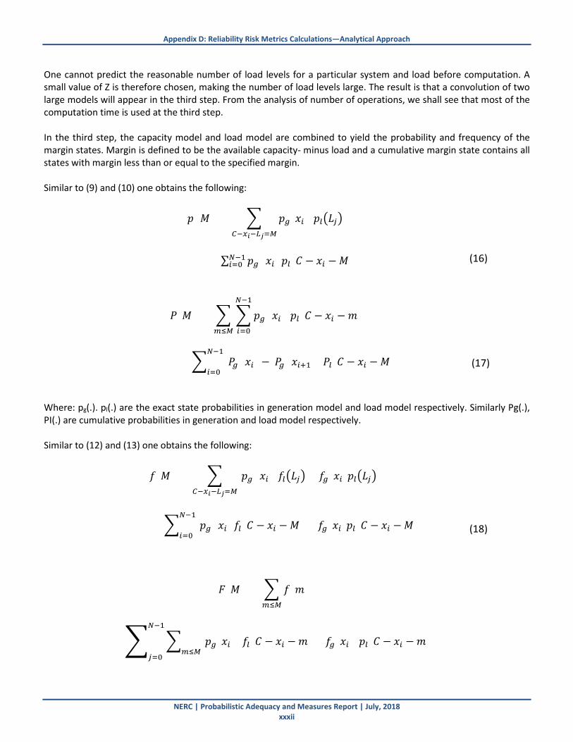
Appendix D: Reliability Risk Metrics Calculations—Analytical Approach
NERC | Probabilistic Adequacy and Measures Report | July, 2018 xxxii
One cannot predict the reasonable number of load levels for a particular system and load before computation. A small value of Z is therefore chosen, making the number of load levels large. The result is that a convolution of two large models will appear in the third step. From the analysis of number of operations, we shall see that most of the computation time is used at the third step. In the third step, the capacity model and load model are combined to yield the probability and frequency of the margin states. Margin is defined to be the available capacity- minus load and a cumulative margin state contains all states with margin less than or equal to the specified margin. Similar to (9) and (10) one obtains the following:
𝑝𝑝 (𝑀𝑀) = � 𝑝𝑝𝑔𝑔(𝑚𝑚𝑘𝑘)𝐶𝐶−𝑥𝑥𝑖𝑖−𝐿𝐿𝑗𝑗=𝑀𝑀
𝑝𝑝𝑙𝑙�𝐿𝐿𝑗𝑗�
= ∑ 𝑝𝑝𝑔𝑔 (𝑚𝑚𝑘𝑘)𝑁𝑁−1
𝑘𝑘=0 𝑝𝑝𝑙𝑙(𝐶𝐶 − 𝑚𝑚𝑘𝑘 − 𝑀𝑀)
(16)
𝐿𝐿 (𝑀𝑀) = � �𝑝𝑝𝑔𝑔 (𝑚𝑚𝑘𝑘)𝑁𝑁−1
𝑘𝑘=0
𝑚𝑚≤𝑀𝑀
𝑝𝑝𝑙𝑙(𝐶𝐶 − 𝑚𝑚𝑘𝑘 − 𝑚𝑚)
= � (𝐿𝐿𝑔𝑔 (𝑚𝑚𝑘𝑘)𝑁𝑁−1
𝑘𝑘=0− 𝐿𝐿𝑔𝑔 (𝑚𝑚𝑘𝑘+1)) 𝐿𝐿𝑙𝑙(𝐶𝐶 − 𝑚𝑚𝑘𝑘 − 𝑀𝑀)
(17)
Where: pg(.). pl(.) are the exact state probabilities in generation model and load model respectively. Similarly Pg(.), PI(.) are cumulative probabilities in generation and load model respectively. Similar to (12) and (13) one obtains the following: 𝑖𝑖 (𝑀𝑀) = � [𝑝𝑝𝑔𝑔 (𝑚𝑚𝑘𝑘)
𝐶𝐶−𝑥𝑥𝑖𝑖−𝐿𝐿𝑗𝑗=𝑀𝑀
𝑖𝑖𝑙𝑙�𝐿𝐿𝑗𝑗� + 𝑖𝑖𝑔𝑔(𝑚𝑚𝑘𝑘)𝑝𝑝𝑙𝑙�𝐿𝐿𝑗𝑗�]
= � [𝑝𝑝𝑔𝑔 (𝑚𝑚𝑘𝑘)𝑁𝑁−1
𝑘𝑘=0𝑖𝑖𝑙𝑙(𝐶𝐶 − 𝑚𝑚𝑘𝑘 − 𝑀𝑀) + 𝑖𝑖𝑔𝑔(𝑚𝑚𝑘𝑘)𝑝𝑝𝑙𝑙(𝐶𝐶 − 𝑚𝑚𝑘𝑘 −𝑀𝑀)]
(18)
𝐹𝐹 (𝑀𝑀) = � 𝑖𝑖(𝑚𝑚)𝑚𝑚≤𝑀𝑀
= � � [𝑝𝑝𝑔𝑔(𝑚𝑚𝑘𝑘 )𝑚𝑚≤𝑀𝑀
𝑖𝑖𝑙𝑙(𝐶𝐶 − 𝑚𝑚𝑘𝑘 − 𝑚𝑚) +𝑁𝑁−1
𝑗𝑗=0
𝑖𝑖𝑔𝑔(𝑚𝑚𝑘𝑘 ) 𝑝𝑝𝑙𝑙(𝐶𝐶 − 𝑚𝑚𝑘𝑘 − 𝑚𝑚)]
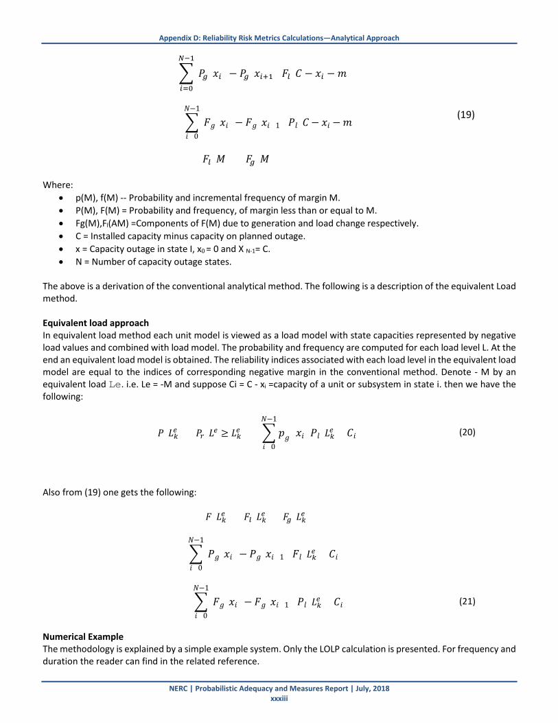
Appendix D: Reliability Risk Metrics Calculations—Analytical Approach
NERC | Probabilistic Adequacy and Measures Report | July, 2018 xxxiii
= �[𝐿𝐿𝑔𝑔(𝑚𝑚𝑘𝑘)𝑁𝑁−1
𝑘𝑘=0
− 𝐿𝐿𝑔𝑔(𝑚𝑚𝑘𝑘+1)]𝐹𝐹𝑙𝑙(𝐶𝐶 − 𝑚𝑚𝑘𝑘 − 𝑚𝑚)
+ � [𝐹𝐹𝑔𝑔(𝑚𝑚𝑖𝑖)𝐷𝐷−1
𝑖𝑖=0− 𝐹𝐹𝑔𝑔(𝑚𝑚𝑖𝑖+1)]𝐿𝐿𝑙𝑙(𝐶𝐶− 𝑚𝑚𝑖𝑖 −𝑚𝑚)
= 𝐹𝐹𝑙𝑙(𝑀𝑀) + 𝐹𝐹𝑔𝑔(𝑀𝑀)
(19)
Where:
• p(M), f(M) -- Probability and incremental frequency of margin M. • P(M), F(M) = Probability and frequency, of margin less than or equal to M. • Fg(M),Fl(AM) =Components of F(M) due to generation and load change respectively. • C = Installed capacity minus capacity on planned outage. • x = Capacity outage in state I, x0 = 0 and X N-1= C. • N = Number of capacity outage states.
The above is a derivation of the conventional analytical method. The following is a description of the equivalent Load method. Equivalent load approach In equivalent load method each unit model is viewed as a load model with state capacities represented by negative load values and combined with load model. The probability and frequency are computed for each load level L. At the end an equivalent load model is obtained. The reliability indices associated with each load level in the equivalent load model are equal to the indices of corresponding negative margin in the conventional method. Denote - M by an equivalent load Le. i.e. Le = -M and suppose Ci = C - xi =capacity of a unit or subsystem in state i. then we have the following:
𝐿𝐿(𝐿𝐿𝑘𝑘𝑒𝑒 ) = 𝐿𝐿𝑟𝑟(𝐿𝐿𝑒𝑒 ≥ 𝐿𝐿𝑘𝑘𝑒𝑒 ) = �𝑝𝑝𝑔𝑔 (𝑚𝑚𝑖𝑖)
𝐷𝐷−1
𝑖𝑖=0𝐿𝐿𝑙𝑙(𝐿𝐿𝑘𝑘𝑒𝑒 + 𝐶𝐶𝑖𝑖) (20)
Also from (19) one gets the following:
𝐹𝐹(𝐿𝐿𝑘𝑘𝑒𝑒 ) = 𝐹𝐹𝑙𝑙(𝐿𝐿𝑘𝑘𝑒𝑒 ) + 𝐹𝐹𝑔𝑔(𝐿𝐿𝑘𝑘𝑒𝑒 )
= � [𝐿𝐿𝑔𝑔(𝑚𝑚𝑖𝑖)𝐷𝐷−1
𝑖𝑖=0−𝐿𝐿𝑔𝑔(𝑚𝑚𝑖𝑖+1)]𝐹𝐹𝑙𝑙(𝐿𝐿𝑘𝑘𝑒𝑒 + 𝐶𝐶𝑖𝑖)
+ � [𝐹𝐹𝑔𝑔(𝑚𝑚𝑖𝑖)𝐷𝐷−1
𝑖𝑖=0−𝐹𝐹𝑔𝑔(𝑚𝑚𝑖𝑖+1)]𝐿𝐿𝑙𝑙(𝐿𝐿𝑘𝑘𝑒𝑒 + 𝐶𝐶𝑖𝑖)
(21)
Numerical Example The methodology is explained by a simple example system. Only the LOLP calculation is presented. For frequency and duration the reader can find in the related reference.
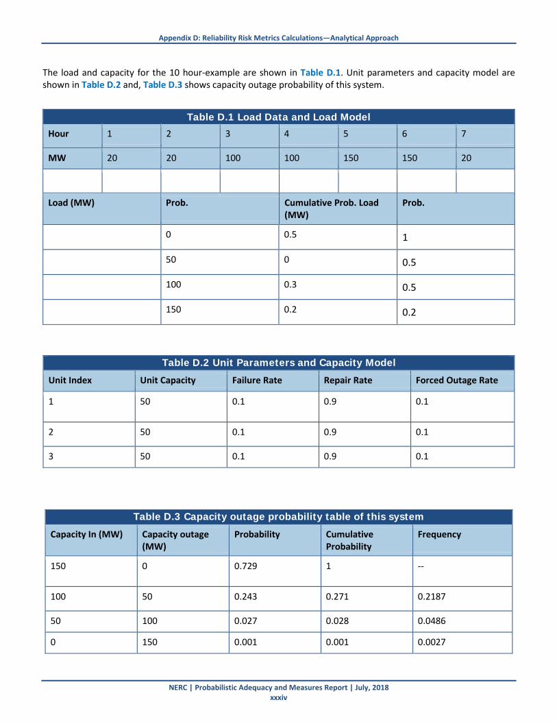
Appendix D: Reliability Risk Metrics Calculations—Analytical Approach
NERC | Probabilistic Adequacy and Measures Report | July, 2018 xxxiv
The load and capacity for the 10 hour-example are shown in Table D.1. Unit parameters and capacity model are shown in Table D.2 and, Table D.3 shows capacity outage probability of this system.
Table D.1 Load Data and Load Model
Hour 1 2 3 4 5 6 7
MW 20 20 100 100 150 150 20
Load (MW) Prob. Cumulative Prob. Load (MW)
Prob.
0 0.5 1
50 0 0.5
100 0.3 0.5
150 0.2 0.2
Table D.2 Unit Parameters and Capacity Model
Unit Index Unit Capacity Failure Rate Repair Rate Forced Outage Rate
1 50 0.1 0.9 0.1
2 50 0.1 0.9 0.1
3 50 0.1 0.9 0.1
Table D.3 Capacity outage probability table of this system
Capacity In (MW) Capacity outage (MW)
Probability Cumulative Probability
Frequency
150 0 0.729 1 --
100 50 0.243 0.271 0.2187
50 100 0.027 0.028 0.0486
0 150 0.001 0.001 0.0027

Appendix D: Reliability Risk Metrics Calculations—Analytical Approach
NERC | Probabilistic Adequacy and Measures Report | July, 2018 xxxv
System Margin The density function of system available capacity C(Y) where Y is a random variable representing the system available capacity in MW. If we define generation margin as the amount by which the system available capacity exceed the system peak load on any day, then the following:
(Generation) Margin = Available Capacity – (Daily peak) Load
The Generation margin is also a random variable, Z, in MW with the relationship as follows:
Z= Y- X The probability density of system margin, M(Z), must be determined from the densities of load and capacity. The System Margin can be a discrete or continuous random variable. One can discretize the load density by dividing it into a number of discrete intervals. This results in a discrete approximation to the continuous margin density. The accuracy of the discrete margin approximation is improved by selecting a large number of intervals of small MW size. Discrete System Margin Density A full Binomial Capacity model is used for illustration. Since the load and available capacity random variables are independent, the Margin density is given by the following relationship:
𝑀𝑀(𝑍𝑍) = �𝐶𝐶(𝑌𝑌)𝐿𝐿(𝑌𝑌 − 𝑍𝑍)𝑌𝑌
Where for each value of Z the summation is taken over all values of available capacity, Y. As describe in previous Equations Reliability Indices Computation is performed by combining the capacity model with the load model to obtain a probabilistic model of system capacity adequacy. Using Conventional Analytical Method We can get the Marginal distribution based on the load and capacity distribution previously calculated. This is the marginal state matrix. See Table D.4.
Table D.4 Marginal State Matrix
Load 0 MW Prob. 0.5
Load 100 MW Prob. 0.3
Load 150 MW Prob. 0.2
Cap In 150 MW Cap Out 0 MW , Prob. 0.729 150 MW 50 MW 0 MW Cap In 100 MW Cap Out 50 MW, Prob. 0.243 100 MW 0 MW -50 MW Cap In 50 MW Cap out 100 MW, Prob. 0.027 50 MW -50 MW -100 MW Cap In 0 MW Cap Out 150 MW, Prob. 0.001 0 MW -100 MW -150 MW
The probability associated with each marginal state is shown in Table D.5.

Appendix D: Reliability Risk Metrics Calculations—Analytical Approach
NERC | Probabilistic Adequacy and Measures Report | July, 2018 xxxvi
Table D.5 Marginal State Probability Matrix Load 0 MW Load 100 MW Load 150 MW 0.5 0.3 0.2
Cap In 150 MW 0.729 0.3645 0.2187 0.1458 Cap In 100 MW 0.243 0.1215 0.0729 0.0486 Cap In 50 MW 0.027 0.0135 0.0081 0.0054 Cap In 0 MW 0.001 0.0005 0.0003 0.0002
The marginal distribution is calculated in Table D.6.
Table D.6 Marginal Distribution Margin (MW) (Cap in , Load) Pair Prob. Cumulative Prob.
150 (150, 0) 0.3645 1 100 (100,0) 0.1215 0.6355 50 (50, 0), (150, 100) 0.2322 0.5140 0 (0, 0), (100, 100), (150, 150) 0.2192 0.2818 -50 (50, 100), (100, 150) 0.0567 0.0626 -100 (0, 100), (50, 150) 0.0057 0.0059 -150 (0, 150) 0.0002 0.0002
Using Equivalent Load Method In a large system the number of state of both load model and capacity model usually are large. So the marginal state matrix is a large two dimensional matrix. In the equivalent load method we can avoid to calculate the each element of this large two Dimension matrix. Instead the marginal distribution is calculated by convolving one unit capacity mode at a time. This successive updating of marginal distribution started with the original load distribution. The right three columns in the Table D.7 show the marginal distribution after adding each unit.
Table D.7 Equivalent Load Distribution Equivalent Load Cumulative of
Original Load Cumulative Prob. After Unit #1
Cumulative Prob. After Unit #2
Cumulative Prob. After Unit #3
-150 1 1 1 1 -100 1 1 1 0.6355 -50 1 1 0.595 0.514 0 1 0.55 0.505 0.2818 50 0.5 0.5 0.257 0.0626 100 0.5 0.23 0.041 0.0059 150 0.2 0.02 0.002 0.0002
The last column in Table D.6 shows the margin state distribution calculated by using the conventional method. The last column in Table D.7 shows the margin state distribution calculated by using the equivalent load approach. They produce identical results. But the computation time in conventional method increases exponentially with the size of the system, while the computation time increases linearly in the equivalent load approach [1].
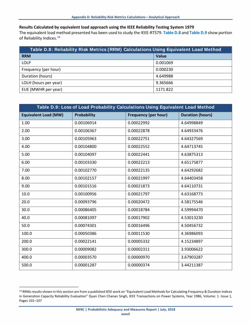
Appendix D: Reliability Risk Metrics Calculations—Analytical Approach
NERC | Probabilistic Adequacy and Measures Report | July, 2018 xxxvii
Results Calculated by equivalent load approach using the IEEE Reliability Testing System 1979 The equivalent load method presented has been used to study the IEEE-RTS79. Table D.8 and Table D.9 show portion of Reliability Indices.14
Table D.8: Reliability Risk Metrics (RRM) Calculations Using Equivalent Load Method RRM Value LOLP 0.001069 Frequency (per hour) 0.000230 Duration (hours) 4.649988 LOLH (hours per year) 9.365666 EUE (MWHR per year) 1171.822
Table D.9: Loss of Load Probability Calculations Using Equivalent Load Method
Equivalent Load (MW) Probability Frequency (per hour) Duration (hours)
1.00 0.00106914 0.00022992 4.64998849
2.00 0.00106367 0.00022878 4.64933476
3.00 0.00105963 0.00022751 4.64327569
4.00 0.00104800 0.00022552 4.64713745
5.00 0.00104097 0.00022441 4.63875313
6.00 0.00103330 0.00022213 4.65175877
7.00 0.00102770 0.00022135 4.64292682
8.00 0.00102157 0.00021997 4.64403458
9.00 0.00101516 0.00021873 4.64110731
10.0 0.00100956 0.00021797 4.63168773
20.0 0.00093796 0.00020472 4.58175546
30.0 0.00086405 0.00018784 4.59994470
40.0 0.00081097 0.00017902 4.53013230
50.0 0.00074301 0.00016496 4.50456732
100.0 0.00050386 0.00011530 4.36986093
200.0 0.00022141 0.00005332 4.15234897
300.0 0.00009082 0.00002311 3.93006622
400.0 0.00003570 0.00000970 3.67903287
500.0 0.00001287 0.00000374 3.44211387
14 RRMs results shown in this section are from a published IEEE work on “Equivalent Load Methods for Calculating Frequency & Duration Indices in Generation Capacity Reliability Evaluation” Quan Chen Chanan Singh, IEEE Transactions on Power Systems, Year 1986, Volume: 1. Issue 1, Pages 101–107

NERC | Probabilistic Adequacy and Measures Report| July, 2018 38
Appendix E: Additional Resource Adequacy Metric Conditional Value at Risk (CVaR) Conditional Value at Risk (CVaR) measures the expected (weighted average) outcome of tail-end events. It is commonly used in the financial sector to minimize economic risk when developing investment portfolios. For power system applications, CVaRα is used to assess the expected value of the α-percent worst outcomes. For example, the CVaR95 metric measures the expected curtailment magnitude over the worst five percent of potential outcomes. It has a very desirable mathematical property, namely that it is coherent,15 which means that it satisfies the properties of monotonicity, sub-additivity, homogeneity, and translational invariance. As a continuous function it is readily incorporated into convex and linear programing optimization models, e.g. the objective function minimizes CVaR (risk). CVaR is currently used by Power Systems Research, Inc. in Brazil.16 The Northwest Power and Conservation Council also uses this variable as a cost risk measure in its system expansion model.17 Viable system expansion plans for the Pacific Northwest are those with the lowest expected cost over the 10 percent highest cost years (CVaR90). The Council is currently considering using CVaR as a potential adequacy metric.18 Definition Conditional Value at Risk (CVaRα), as a power supply adequacy metric, is the probability-weighted average value of the lowest surplus (capacity minus load) over the (100 – α) percentile of possible outcomes (where α typically ranges from 90 to 99). Generally, it is defined as the conditional expected surplus of all outcomes less than or equal to the Value at Risk (VaRα), which is defined as the surplus value at the (100 – α) percentile. CVaR can be assessed using either Monte-Carlo or Probability-Convolution methods, depending on which is more appropriate.
Simple Numeric Example Suppose a Monte-Carlo simulation produces the following 100 sorted results: {-100, -99, -98… -1}, with each result being equally likely. For an α-threshold of 95 percent, the results of interest are the lowest 5 percent, namely {-100, -99, -98, -97, -96}. For this α-threshold, there is a 5 percent chance that a result will be equal to or less than -96, thus the corresponding VaR95 value is -96. CVaR95 then is the average of all of the values from this distribution that are equal to or less than VaR95. Thus, for this example, CVaR95 = (– 100 – 99 – 98 – 97 – 96) / 5 = – 98. CVaR Calculation for a Monte-Carlo approach For a Monte-Carlo approach, the lowest peak-hour surplus from each simulation is recorded. These surplus values are then sorted from lowest to highest. CVaRα is the average of the surplus values that are less than or equal to VaRα, that is, those that fall into the (100 – α) percentile. Therefore, see the following:
𝐿𝐿𝑚𝑚𝑅𝑅𝛼𝛼 = �𝐸𝐸𝑘𝑘𝐷𝐷𝛼𝛼
𝑁𝑁𝛼𝛼
𝑘𝑘=1
15 “Optimization of Conditional Value at Risk,” R. Tyrrell Rockafellar, Stanislav Uryasev https://sites.math.washington.edu/~rtr/papers/rtr179-CVaR1.pdf 16 “Stochastic Programming Models for Energy Planning,” PSR, Mario Veiga Pereira, June 27, 2016 https://icsp2016.sciencesconf.org/file/251300 17 Seventh Northwest Conservation and Electric Power Plan, February 10, 2016, https://www.nwcouncil.org/media/7149906/7thplanfinal_appdixl_rpm.pdf 18 “Review of Supply Adequacy Criteria in the Northwest,” Power Systems Research, Inc., August 2011 https://www.nwcouncil.org/media/10358/vfinal_Review_of_Power_SupplyAdequacy_Criteria_in_the_Northwest_Region.pdf

Appendix E: Additional Resource Adequacy Metric
NERC | Probabilistic Adequacy and Measures Report | July, 2018 xxxix
where:
• α = Percentage used to define the values at risk, e.g. those in the (100 – α) percentile,
• Si = Surplus (capacity minus load) for the ith simulation,
• N = Number of Simulations,
• Nα = Simulation number of the (100 – α) percentile of N.
Table E.1 below shows sorted surplus values from a created 100-simulation data set that includes the NERC sample data (containing only five simulations). The VaR95 is the surplus value for the 5th percentile of the sorted simulations. For this example Nα is 5. Thus, VaR95 is –2458 megawatts and CVaR95 is –2528 megawatts (the average surplus of simulations 1 through 5). Figure E.1 illustrates VaR95 and CVaR95 graphically.
Table E.1: Surplus Outcomes for a Monte-Carlo Simulation
Simulation Surplus
1 -2598 2 -2563 3 -2528 4 -2493 5 -2458 VaR95 6 -2423 7 -2388 : :
13 -2166 NERC Data : :
16 -2066 NERC Data : :
28 -1660 NERC Data : :
32 -1522 NERC Data : :
37 -1344 NERC Data : :
99 843 100 878

Appendix E: Additional Resource Adequacy Metric
NERC | Probabilistic Adequacy and Measures Report | July, 2018 xl
Figure E.1: Sorted Surplus Values from a Monte-Carlo Simulation
For a Probability-Convolution approach, CVaRα is calculated as the probability-weighted average surplus for those values equal to or less than VaRα (see Figure E.2 for an example of α = 95 percent).
Figure E.2: VaR95 and CVaR95 for a Probability Density Distribution
CVaR Calculation for a Probability-Convolution Approach The general expression for CVaR using a Probability-Convolution method is provided below. This method works well if the probability density distribution for surplus is well defined. CVaRα is the definite integral evaluated from minus infinity to VaRα of the surplus S times the probability density function P(S), divided by the definite integral of the probability density function over the same limits.
-4000
-3000
-2000
-1000
00 5 10 15 20 25 30 35 40
Meg
awat
tsSimulation Index (First 40)
VaR95-2458
CVaR95-2528
NERC Data

Appendix E: Additional Resource Adequacy Metric
NERC | Probabilistic Adequacy and Measures Report | July, 2018 xli
𝐶𝐶𝐿𝐿𝑚𝑚𝑅𝑅𝛼𝛼 = 𝐿𝐿[𝐸𝐸 | 𝐸𝐸 ≤ 𝐿𝐿𝑚𝑚𝑅𝑅𝛼𝛼 ] = ∫ 𝐸𝐸 ∙ 𝑝𝑝(𝐸𝐸) 𝑑𝑑𝐸𝐸𝑉𝑉𝑎𝑎𝑅𝑅𝛼𝛼−∞Pr[ 𝐸𝐸 ≤ 𝐿𝐿𝑚𝑚𝑅𝑅𝛼𝛼] =
1
1 − � 𝛼𝛼100�
� 𝐸𝐸 ∙ 𝑝𝑝(𝐸𝐸) 𝑑𝑑𝐸𝐸
𝑉𝑉𝑎𝑎𝑅𝑅𝛼𝛼
−∞
where: S = Surplus (capacity minus load), P(S) = Probability density distribution for surplus, VaRα = Surplus for which the area under the probability curve from minus infinity to VaR is α. From the load and generation sample data provided by NERC, the highest hourly deficit for each day is selected from the 5-day hourly surplus/deficit data. The collected daily data are sorted as follows (-2,166, -2,056, -1,660, -1,522, -1344) and their populations are calculated using a 500-MW bin, which are listed in Table E.2.
Table E.2: Surplus Population Distribution Left Bin Boundary (MW) Right Bin Boundary (MW) Population
-2,600 -2,100 1 -2,100 -1,600 2 -1,600 -1,100 2
However, CVaR analysis requires more than three data points and ideally should include a few hundred data points. Therefore, a Gaussian function has been derived
𝑖𝑖(𝐸𝐸) = 𝐴𝐴 exp �−(𝐸𝐸 − �̅�𝐸)2
2𝜎𝜎2 �
where A = 2.2, s-bar = -1350 and σ = 570 to closely fit these three points and provide enough data to properly calculate CVaR. The Gaussian function and the three data points are plotted in Figure E.3 below.
Figure E.3: Gaussian Function Fit (red curve) to the NERC Surplus Data Bins (blue squares)
To enable further CVaR analysis, the Gaussian f(s) is transformed into a probability density p(s) by normalization,
0
0.5
1
1.5
2
2.5
-4000 -3000 -2000 -1000 0 1000 2000Popu
latio
n in
Sur
plus
Bin
Surplus (MW)
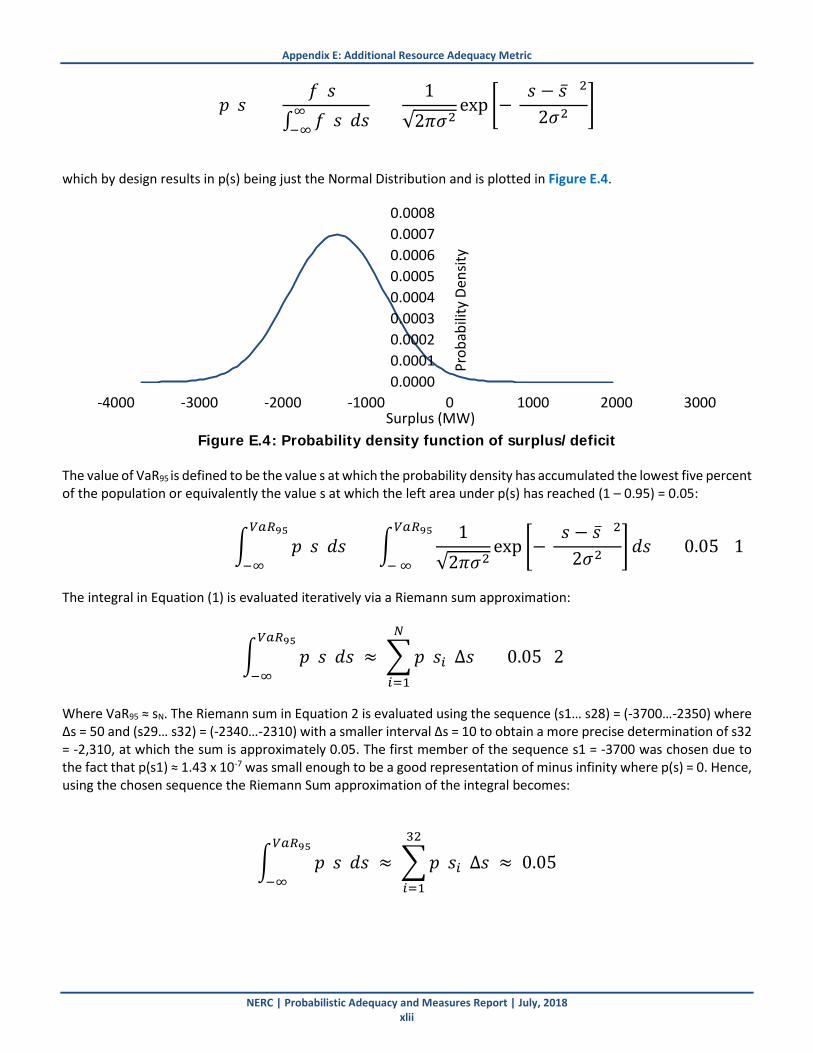
Appendix E: Additional Resource Adequacy Metric
NERC | Probabilistic Adequacy and Measures Report | July, 2018 xlii
𝑝𝑝(𝐸𝐸) = 𝑖𝑖(𝐸𝐸)
∫ 𝑖𝑖(𝐸𝐸)𝑑𝑑𝐸𝐸∞−∞
= 1
√2𝜋𝜋𝜎𝜎2exp �−
(𝐸𝐸 − �̅�𝐸 )2
2𝜎𝜎2 �
which by design results in p(s) being just the Normal Distribution and is plotted in Figure E.4.
Figure E.4: Probability density function of surplus/deficit
The value of VaR95 is defined to be the value s at which the probability density has accumulated the lowest five percent of the population or equivalently the value s at which the left area under p(s) has reached (1 – 0.95) = 0.05:
� 𝑝𝑝(𝐸𝐸)𝑑𝑑𝐸𝐸 = �1
√2𝜋𝜋𝜎𝜎2exp �−
(𝐸𝐸 − �̅�𝐸 )2
2𝜎𝜎2 �𝑉𝑉𝑎𝑎𝑅𝑅95
− ∞𝑑𝑑𝐸𝐸 = 0.05
𝑉𝑉𝑎𝑎𝑅𝑅95
−∞(1)
The integral in Equation (1) is evaluated iteratively via a Riemann sum approximation:
� 𝑝𝑝(𝐸𝐸)𝑑𝑑𝐸𝐸 ≈ �𝑝𝑝(𝐸𝐸𝑘𝑘)∆𝐸𝐸𝑁𝑁
𝑘𝑘=1
= 0.05 (2)𝑉𝑉𝑎𝑎𝑅𝑅95
−∞
Where VaR95 ≈ sN. The Riemann sum in Equation 2 is evaluated using the sequence (s1… s28) = (-3700…-2350) where ∆s = 50 and (s29… s32) = (-2340…-2310) with a smaller interval ∆s = 10 to obtain a more precise determination of s32 = -2,310, at which the sum is approximately 0.05. The first member of the sequence s1 = -3700 was chosen due to the fact that p(s1) ≈ 1.43 x 10⁻⁷ was small enough to be a good representation of minus infinity where p(s) = 0. Hence, using the chosen sequence the Riemann Sum approximation of the integral becomes:
� 𝑝𝑝(𝐸𝐸)𝑑𝑑𝐸𝐸 ≈ �𝑝𝑝(𝐸𝐸𝑘𝑘)∆𝐸𝐸32
𝑘𝑘=1
≈ 0.05𝑉𝑉𝑎𝑎𝑅𝑅95
−∞
0.00000.00010.00020.00030.00040.00050.00060.00070.0008
-4000 -3000 -2000 -1000 0 1000 2000 3000
Prob
abili
ty D
ensit
y
Surplus (MW)

Appendix E: Additional Resource Adequacy Metric
NERC | Probabilistic Adequacy and Measures Report | July, 2018 xliii
Then VaR95 ≈ 0.05, then Var95 ≈ s32 = -2310. Finally, CVaR95 is just the p(s)-weighted average of s in the interval from minus infinity to VaR95 and is calculated as follows:
𝐶𝐶𝐿𝐿𝑚𝑚𝑅𝑅95 = ∫ 𝐸𝐸 ∙ 𝑝𝑝(𝐸𝐸)𝑑𝑑𝐸𝐸𝑉𝑉𝑎𝑎𝑅𝑅95−∞
∫ 𝑝𝑝(𝐸𝐸)𝑑𝑑𝐸𝐸𝑉𝑉𝑎𝑎𝑅𝑅95−∞
= ∫ 𝐸𝐸 ∙ 𝑝𝑝(𝐸𝐸)𝑑𝑑𝐸𝐸−2310−∞
0.05 ≈ −2528 (3)