Private Labels and Retailer Profitability:

Bilateral Bargaining in the Grocery Channel∗

Paul B. Ellicksona, Pianpian Konga, and Mitchell J. Lovetta

aSimon Business School, University of Rochester

May 19, 2017

Abstract

We examine the role of store branded “private label” products in determining bargaining outcomesbetween retailers and manufacturers in the brew-at-home coffee category. Exploiting a novel setting inwhich the dominant, single-serve technology was protected by a patent preventing private label entry,we develop a structural model of demand and supply-side bargaining and seek to quantify the impact ofprivate labels on retailer profits. To quantify the benefits of private label introduction, we decomposetheir impact into the direct profits (from adding an additional product type) and the bargaining benefiton branded products (from increasing bargaining leverage), netting out the business stealing effects onincumbent branded products. We find that bargaining outcomes are driven primarily by bargainingleverage, while bargaining ability is relatively symmetric between retailer and manufacturer. Moreover,the impact of bargaining leverage is substantial: bargaining benefits account for roughly 20% of the over-all benefit of private label introduction, which is itself on the order of 10% of pre-introduction profits.Finally, we find that private labels are beneficial to all retailers, but some retailers gain much more thanothers.

Keywords: Retail Grocery, Bargaining Models, Private Labels, Store Brands, Demand Estimation.

∗We thank Guy Arie, Greg Crawford, Ron Goettler, Paul Grieco and Ali Yurukoglu for valuable comments.We also thank seminar participants at Arizona State Carey, Duke Fuqua, Goethe Universitat, Houston, North-western Kellogg, Penn State economics, Yale SOM and the University of Zurich for helpful feedback. Sendany correspondence to paul.ellickson@simon.rochester.edu (Ellickson), mitch.lovett@simon.rochester.edu (Lovett) orpianpian.kong@simon.rochester.edu (Kong).

1

1 Introduction

Store brands are a key source of profits for many retailers. Unlike their nationally branded counterparts,

the price and positioning of store brands (also referred to as “private labels”) are entirely controlled by the

retailer. This gives store brands a unique strategic role in negotiations with manufacturers, helping determine

the split of overall channel profits (Scott Morton and Zettelmeyer, 2004). In this paper, we examine the

role of private label products in the growth and profitability of the single-cup coffee category. We exploit

a unique setting in which the dominant branded product, Keurig/GMCR’s ‘K-Cup’ technology, was patent

protected, effectively preventing entry by private label products prior to patent expiration. Therefore,

we are able to observe how retailers and manufacturers behave both with and without competition from

private label products, and isolate the factors that change this conduct. To leverage this unique source of

exogenous variation, we build a model of consumer demand and supply-side bargaining in the brew-at-home

coffee category. We estimate the model using weekly, chain-level data from 72 retail market areas. We then

conduct counterfactual exercises aimed at quantifying the impact of private label products on overall channel

profits.

Private labels occupy an important position in the retail landscape. In 2012, private labels accounted for

$98 billion in U.S. food and grocery revenues and 17.1% of total sales (Schultz, 2012; Nielsen Global Survey,

2012). The success of private label programs varies across retailers and categories, with some retailers

(e.g. Wegmans, Whole Foods) making store brands a centerpiece of their overall positioning strategy and

others choosing to focus more intensively on branded goods (e.g. Gelson’s). Heterogeneity in the quality

of private label programs across retailers creates an additional source of variation that is useful in pinning

down the impact of private label entry on bargaining outcomes. Better private labels give retailers a stronger

bargaining position.

Private label products create value along four distinct dimensions. First, they typically offer higher

margins (to the retailer), as they can often be procured in relatively competitive upstream markets (where

manufacturers cannot extract as much rent from the value of their brands). Second, since private labels are

typically priced low relative to their national counterparts, they may expand the overall category by bringing

in consumers with lower willingness to pay. Third, store brands may be important in building store loyalty

and increasing overall traffic by shifting the value proposition from what is on the shelves, to the brand of

the store itself (i.e. changing the scarce resource from the brand of the product to the banner of the store).

Fourth, they can provide the retailer with a stronger bargaining position vis a vis the manufacturers of the

national brands. By giving the retailer a stronger threat point (replacing the national brand with their own

store brand), private labels increase the retailer’s disagreement payoff. This then allows them to extract a

2

larger share of the surplus, especially for the branded products that compete most directly with the store

brand. In this study, we control econometrically for the first two motives, and focus our analysis on the

fourth (bargaining outcomes), while our data requires us to abstract away from the third (increased traffic).

We seek to quantify the factors that influence the retailer-manufacturer bargaining outcome, and understand

how channel profits adjust to the introduction of private label competition.

Our empirical strategy involves exploiting a unique setting that unfolded in the brew-at-home coffee

market over our sample period. A previously mature product category, the brew-at-home coffee market

was disrupted in the mid-to-late 2000s by a new product offering: single-serving coffee pods. The new

technology offered convenience, and a standardized, high-quality brewing experience, to a growing segment

of coffee connoisseurs. While single-serve coffee had existed both in the U.S. and abroad for many years,

Keurig/GMCR was able to position itself as the de facto U.S. standard by offering a wide range of sub-brands

and licensed/partner products, alongside a design that was superior to its rivals and much wider product

distribution.1 Moreover, since both the brewers and K-Cups were patented, competitive entry (to this

particular design) was effectively foreclosed until 2012, creating a unique “before and after experiment”. To

exploit this unique source of variation, we develop a structural model of demand and supply that can control

for confounding factors in the competitive environment (e.g. cost changes, new product entries, continued

market expansion, and evolving substitution patterns) and reveal how private labels changed bargaining

outcomes.

While providing a unique setting for analyzing private label competition, the single-serve coffee category

creates some challenges on the demand side. First, a central aspect of the Keurig/GMCR strategy was

product variety, so it will be important to include the full set of brands they offered. Second, since this was a

new product launch (that we observe almost from inception), K-Cups simply weren’t available in all stores in

all periods. The rollout of products occurred slowly at first, and was focused on particular markets. Finally,

brewing single-cup pods requires owning relatively expensive and specialized hardware. Consumers that did

not own the brewer were not in the market for single-cup pods. Ignoring these market features could lead to

large biases in our demand estimates. Getting the demand system right is critical, as it drives all subsequent

inference. We address all three concerns by developing a random-coefficient, discrete-choice demand system

that accounts for availability and machine ownership by simulating individual consumers and aggregating

up to observable shares (availability and ownership are tied to the data via aggregate moments of each). We

are also able to include the full set of products. We demonstrate that the model yields flexible substitution

patterns that match the evolution of the market.

1Keurig/GMCR is also the “category captain” in many retailers, adding to its dominant position (Nijs et al., 2013). Thecategory captain coordinates with the retailer to manage the selection and display of a given product category. It is typicallyone of the leading national brands.

3

Turning to the supply side, we must first recover wholesale prices, which are not observed in the data.

To do so, we use the first order conditions from the retailer’s profit maximization problem to solve for

the wholesale prices that rationalize retailer decisions (Bresnahan, 1987; Werden and Froeb, 1994). These

inferred wholesale prices are the focus of our bargaining model. We assume that retailers and manufacturers

bargain over linear contracts that determine these “transfer prices.” Following the recent literature on applied

bargaining, we model the retailer-manufacturer vertical contracting relationship as a ‘Nash in Nash’ bargain,

focused on determining the wholesale price that effectively splits the gains from trade. Using the inferred

wholesale prices, we then recover the bargaining parameters and supplier cost parameters that rationalize the

data. To do so, we compute both the profits that each party achieves under agreement and the profits that

would obtain should they fail to reach agreement. Private label products provide a key source of variation

in the disagreement payoffs. We find that, while bargaining ability is relatively symmetric across retailers

and manufacturers, the addition of private labels can change the retailer’s bargaining leverage dramatically,

thereby improving the retailer’s bargaining outcome. In particular, the introduction of a private label product

increases segment profits by about 10% on average, though some firms gain substantially more. Roughly

20% of this lift is due to better terms of trade on the incumbent branded products, a significant indirect

benefit of introducing the new product line.

Our research relates to several streams of literature in both marketing and economics. First, we contribute

to the literature on private labels, which includes the seminal papers by Hoch and Banerji (1993) and Dhar

and Hoch (1997) that identified and cataloged the determinants of private label success, and sought to

explain why their penetration varied across retailers. Pauwels and Srinivasan (2004) examine the impact of

store brands on the relative profitability of retailers and suppliers, as well as their role in shifting consumer

demand, whereas Sayman et al. (2002) study how private labels are positioned vis a vis national brands.

Hansen et al. (2006) investigate whether consumer tastes for store brands are correlated across categories, or

are driven more by category-specific factors. They find strong evidence of the former relative to the latter.

Chintagunta et al. (2002) empirically analyze how private labels change conduct in the channel, as well as

how this conduct translates through to retailer pricing decisions. In the paper most closely related to ours,

Draganska et al. (2010) empirically model the bargaining problem between retailers and manufactures in

the German market for ground coffee, seeking to quantify the sources of heterogeneous bargaining power

and determine whether they have shifted over time. Similarly, Noton and Elberg (2016) model bargaining

between retailers and manufacturers in the Chilean market for instant and ground coffee, focusing on the

impact of supplier size on the split of channel profits. Contrary to conventional wisdom, they find that

small suppliers often attain shares of the channel surplus on par with the largest supplier. Meza and Sudhir

(2010) also examine how private labels change bargaining power (in the breakfast cereal market), and ask

4

whether and how retailers can use prices to strategically influence this negotiation. Finally, Scott Morton

and Zettelmeyer (2004) show how private labels can influence disagreement payoffs, and argue that the

endogenous determination of these quantities can explain the relative positioning decisions of branded firms.

We draw upon the theoretical literature on bilateral Nash bargaining (Nash, 1950; Rubinstein, 1982),

which includes the theoretical development of the ‘Nash in Nash’ bargaining solution by Horn and Wolinsky

(1988), the workhorse model for most applied work.2 In doing so, we contribute to the growing stream of

empirical literature on bargaining models, which includes papers by Misra and Mohanty (2006), Ho (2009),

Draganska et al. (2010), Crawford and Yurukoglu (2012), Grennan (2013), Ho and Lee (2013), Gowrisankaran

et al. (2014), and Crawford et al. (2015). We draw most closely upon the empirical methods proposed by

Grennan (2013). Finally, this work is also related to a broader empirical literature on vertical contracting,

which includes important contributions by Villas-Boas (2007) and Bonnet and Dubois (2010), among several

others. Our central contribution lies in bringing together the two literatures on private labels and bargaining

models, using the bargaining framework to unpack the role of private labels in shaping channel profits. The

natural experiment afforded by the presence, and then expiration, of patent protection allows us to uncover

the causal impact of private labels on bargaining outcomes.

The paper is organized as follows. In section 2, we describe the data used in our empirical study and

provide an overview of the at home coffee market and the role of the single serve (K-Cup) segment in driving

its expansion. The model and estimation are described in section 3. We present the results of our estimation

in section 4 and conduct counterfactual exercises in section 5. Section 6 concludes.

2 Data and Setting

The data are drawn from IRI’s point of sale (POS) database for the period January 2008 to March 2014. The

data cover 72 U.S. retailer-market areas (RMAs) and include over 50 distinct retail banners (e.g. Safeway,

Kroger).3 For each RMA, we observe weekly, SKU-level data on sales, price per serving and merchandising

variables, each aggregated up from the individual store level to the RMA. In addition, we observe the

standard volume (ACV) weighted product distribution measure, our key proxy for product availability at

the store-level. Rather than working with individual SKUs, we aggregate up to the segment-brand level,

so that, for example, all Starbuck’s K-Cup products (e.g. Dark Sumatra, Breakfast Blend) are rolled up

to a single choice. Note that this is done by segment, so that, for example, Starbucks premium drip coffee

(whole bean and ground) is treated as a separate product from the Starbucks K-Cup offering. We include

2The ‘Nash in Nash’ framework has been further micro-founded in recent work by Collard-Wexler et al. (2014)3A retailer-market area is a geographic trading area defined by IRI, which roughly correspond to retailer divisions. Retailer

divisions are usually organized around regional distribution centers, which typically serve a few hundred individual stores.

5

four coffee segments: instant (e.g. Nescafe), main (e.g. Folgers), premium (e.g. Starbucks) and single-cup

(e.g. Keurig). The four segments are vertically differentiated, with instant and main offering the cheapest

alternatives and single-cup the costliest.

In addition to the aggregate POS data, we include cross-tabulations drawn from the IRI individual

panelist data. We use the panelist cross-tabs in two ways. First, the panel provides an estimate of the

number of shoppers in each RMA. We use this to construct our measure of market size. We define the size

of the market to be the number of shoppers times the number of days per week (7) times a scaling factor

related to coffee use in that RMA, which we obtain from the average daily coffee purchases in that market

per shopper. Second, we develop a proxy for the installed base of K-Cup machine owners. We extract K-Cup

penetration data that reports, at the yearly level, the percent of shoppers (in each RMA) who have consumed

K-Cup coffee brands in the previous 12 months. We use these yearly values from the panelist data, along

with weekly machine sales data from the POS data, to impute weekly observations of installed base at the

RMA-weekly level. The details of this imputation are available in the appendix.

Finally, we obtain information on coffee bean commodity prices from the International Coffee Organiza-

tion (http://www.ico.org). These bean prices are available at the monthly level for the four primary coffee

bean types: Colombian milds, other milds, Brazilian naturals, and Robustas. The prices are in US cents

per pound, which we convert to US dollars per pound for our analysis. The prices for all the bean types,

except the Robustas, are closely correlated. The Robustas are priced slightly lower than the other bean

types. During the observation period, the bean prices increase and then fall, with the peak prices occurring

in early 2011.

Our final sample is selected to include RMA-week-segment-brand cases with a reasonable level of distri-

bution. First, we drop cases with less than 10% ACV distribution in the week. We found these observations

to be relatively unreliable. Second, we drop any segment-brand in an RMA if it fails to ever achieve a 50%

median percent ACV distribution (after dropping the cases below 10%). These segment-brands represent rel-

atively small share cases and, with this selection criteria, we retain 87.1% of the total potential observations

and 98.3% of the dollar sales.

2.1 The Brew-At-Home Coffee Market

The previously mature category of coffee for ‘at home’ brewing was disrupted in the mid to late 2000s

by the creation and expansion of the single serving ‘K-Cup’ technology pioneered by Keurig and Green

Mountain Coffee Roasters (GMCR). While a variety of single serve coffee technologies have existed in the

U.S. for quite some time (primarily in the commercial office setting), they did not achieve widespread

6

adoption in the at-home market until Keurig effectively created the de facto standard with its proprietary

K-Cup technology.4 Keurig started by focusing on the commercial office market, utilizing a direct sales

force distribution system that relied on partnerships with five primary coffee roasters, who also handled the

production and distribution of the cups. They shifted focus to the much larger at-home market in the early

2000s, at which point GMCR acquired Keurig (they had earlier been separate companies) and brought the

main coffee roasters in house as well. The popularity of the Keurig system leveraged the growing demand for

premium coffee resulting from the rapid expansion of Starbucks cafes and other premium coffee shops in the

U.S. throughout the 1990s, which also drove the growth of the premium ground and whole bean segment in

the grocery channel in the late 1990s and early 2000s. The Keurig system offered the convenience of a ‘mess-

free’ single-serve brewing experience, while standardizing the quality of the delivered coffee (by precisely

controlling the portion size, brewing time and temperature). A key factor in their positioning strategy

was the wide array of flavors, styles and brands they offered, which GMCR achieved through an aggressive

licensing and partnership strategy with household brands. This positioning differentiated GMCR’s K-Cups

from competing single-serve products like Senseo, Flavia and Tassimo. Moreover, by becoming the de facto

standard for single-serve at-home brewing, they were effectively the only single-cup option available (in wide

distribution) at grocery stores, mass merchandisers and clubs, which created a network effect.

Figure 1a shows the evolution of the four main coffee segments over time. The horizontal axis is delineated

in weeks since the first week of 2008 and ending at the end of the first quarter of 2014. The vertical axis

is national dollar sales of coffee. While there is clear seasonality in sales over the course of any given year,

the stability of the three traditional segments (premium, instant and main) is clear. Main and premium

command relatively equal dollar shares of the overall market, while instant lags far behind. The most

dramatic feature of the graph is the meteoric rise of the single-cup segment, which starts essentially from

scratch in 2008, yet becomes the largest overall segment by the end of the sample period.

Figure 1b focuses on the single-cup segment alone, revealing Keurig’s dominant sales position relative to

its other partners and licensees (before patent expiration) as well as the sharp growth of the private label

brands that entered when the patents expired in September of 2012 (week 246 in the figure).

Figure 2 illustrates how product availability (in all four segments) and installed base (for the single cup

segment) evolved over the sample period. Figure 2a shows the sales weighted percent ACV over time for

all four categories. From the figure, it is clear that the dominant brands in main and instant are essentially

carried everywhere, whereas premium, with its more regionally-focused local brands (Bronnenberg et al.,

2012), is more heterogeneous (the lower level of average availability in the premium segment mainly reflects

4In Europe, the capsule-based single-cup espresso brewing system developed by Nespresso has become the standard there.Nespresso machines are available in the U.S. as well, but have had more limited success in this market than Keurig due to theirfocus on espresso-based beverages and their far more limited capsule distribution, which is still primarily through online sites.

7

0e+00

1e+07

2e+07

3e+07

100 200 300week

sale

s($)

segmentmainpremiuminstantsingle cup

National Sales ($) 2009−2014Q1

(a) National Coffee Sales by Segment

0e+00

1e+07

2e+07

3e+07

0 100 200 300week

sale

s(cu

p)

brandFOLGERS GOURMETKEURIGMILLSTONEPRIVATE LABELSTARBUCKS

National Sales(Cup) Top Single Cup Brands 2008−2014Q1

(b) Single Cup Product Shares

Figure 1: Coffee Sales

80

90

100

0 26 52 78 104 130 156 182 208 234 260 286 312week

%A

CV

segmentmainpremiuminstantsingle cup

Sales Weighted %ACV trend 2008−2014Q1

(a) Availability (b) Installed base

Figure 2: Availability and Installed Base

variation across chains in what brands they carry, not variation within chains in the products that are carried

in particular stores). Note that, even in premium, availability is clearly quite stable over time. In single cup,

however, availability increases sharply for roughly the first third of the sample, but stabilizes by the end.

This is due to the progressive nature of the K-Cup roll-out and the large number of new product entries

(mainly through partnerships and licensing) that occurred over this period. Our demand model (presented in

section 3.1) has been constructed to account for these features. Figure 2b shows the evolution of our imputed

measure of installed base (percent of the population that own Keurig-compatible brewers) aggregated to the

regional level. As the figure makes clear, the installed base continued to grow over the sample period, and

exhibited substantial geographic variation. These patterns will also be accounted for in our demand analysis.

In total our data contain 72 retail market areas and 53 unique grocery banners. The data span 326 weeks,

but some RMAs are missing data in the first year. As a result, we have 22,116 weekly RMA observations.

The number of segment-brands varies across weeks from 16 to 57 and generally increases over time, as

single-cup brands are added to the product mix. In total, we have 615,424 observations at the RMA-week-

segment-brand level.

8

Table 1 presents summary statistics for the coffee dataset, after aggregating to the RMA-week level. The

first set of columns correspond to the pre-patent expiration period and the second set of columns corresponds

to the post-patent expiration period. The vertical structure of these products (as revealed by their prices)

is clear from this table, as are the relative sizes of the segments (presented here in units; note that dollar

sales were used in figure 1a). Over the sample period, the single-cup segment triples in unit share, while its

average price increases modestly. The distribution (availability, measured using ACV) of all brands grows

over time, but single-cup grows slightly faster. The use of display also increases for the single-cup segment.

The number of brands is relatively constant for the main, premium, and instant segments, but it increases

for the single-cup segment. The reason for the apparent increase includes both the broader distribution of

existing national brands and the introduction of a number of smaller brands into the category, particularly

very late in the time period.

Pre-patent Expiration Post-patent ExpirationSegment Main Premium Instant Single-Cup Main Premium Instant Single-CupFirst Q Price 0.12 0.24 0.14 0.58 0.14 0.26 0.14 0.66Third Q Price 0.16 0.3 0.16 0.7 0.15 0.3 0.16 0.72Avg. Price 0.14 0.28 0.15 0.64 0.15 0.28 0.15 0.69Avg. Share 0.0183 0.00456 0.00447 0.00095 0.01762 0.0047 0.00447 0.00153Segment Share 0.1195 0.0439 0.026 0.0041 0.1111 0.0487 0.0239 0.0169Avg. ACV 84 77 89 70 86 79 93 79Avg. %Display 11.3 9.5 1.3 5.8 13.4 10.7 1.6 10.7First Q NBrands 6 8 5 2 6 9 5 9Third Q NBrands 7 12 6 5 7 13 6 13Avg. #Brands 6.7 10 5.9 3.7 6.5 10.9 5.4 11.2

Table 1: Summary Statistics

2.2 Descriptive Evidence

In this section, we present some descriptive evidence aimed at demonstrating the impact of Keurig’s patent

expiration on prices and market outcomes. The goal is to help demonstrate the scope for identifying shifts

in the determinants of bargaining power, which is the focus of our structural model. Since our main interest

lies in identifying the wholesale price that results from negotiations between retailers and manufacturers, we

focus on regular price as our primary outcome variable.5 Since the POS data do not distinguish between

regular and promotional prices, we proxy for the regular “shelf” price by computing the 90th moving quantile

of quarterly prices and treating this as the regular price. We then ask whether prices fall post-patent. Figure

3a shows the regular price series for the leading brand in each of the three primary segments (single-cup,

5See Nijs et al. (2010) on the role of manufacturer trade promotions.

9

(a) Regular Prices of Leading Brand

Weekly Number of Private Label Entries

Week

Fre

quency

100 150 200 250 300

02

46

810

(b) Private Label Entry Timing

Figure 3: Descriptive Results

premium and main). There is a single price series for each retailer (RMA) in each category. By comparing

across segments, we are able to partly control for changes in the competitive environment that would impact

all three segments equally (e.g. changes in costs, seasonality, and so forth). It is clear from the figure that

prices in the single cup segment decreased after patent expiration (quarter 19 in the figure, corresponding

to the vertical line). Moreover, they continue to fall for the remainder of the sample, as additional private

label and independent (e.g. non-GMCR-affiliated) brands continue to enter the market. We formalize this

by conducting a difference-in-difference analysis between the single-cup segment and the other segments for

the pre- versus post-patent expiration periods. We include controls for time trends, quarter of year dummies

and RMA fixed effects. We find that the interaction representing the diff-in-diff for the immediate decrease

from quarter 19 to 20 is significant (coef=-0.034, se=0.006, n=432), and so is the total decrease in the post

patent expiration (coef=-0.024, se=0.003, n=2592).

The timing of entry by private label brands is shown in Figure 3b, which contains a histogram character-

izing the timing of private label entries over the sample period. Note that while the vast majority of entries

occurred within plus or minus four weeks of patent expiration, there is another group of private label brands

that chose to launch about a year later instead.6

6There are also three entries that occurred long before patent expiration, apparently in violation of the patent. Ourunderstanding is that at least one of these firms was threatened with a lawsuit and subsequently withdrew the related products.

10

3 Model and Estimation

On the demand side, we specify a relatively standard discrete choice, random coefficient model of consumer

demand (aggregated to the market share level) using the framework developed by Berry et al. (1995). To

accommodate the rapid expansion of the single-cup segment (particularly the limited early availability in

many grocery chains) and also to account for the costly hardware requirement of owning a Keurig brewing

system, we employ methods developed by Bruno and Vilcassim (2008) to simulate choice sets that are

consistent with these market features.

On the supply side, we assume that retailers set monopoly prices at the retail level (abstracting away

from retailer to retailer competition).7 Using the first order conditions (FOCs) of the monopoly pricing

problem, we then ‘back out’ the implied marginal costs the retailer pays for each coffee product (Werden and

Froeb (1994); Nevo (2000a)). These costs are assumed to be the wholesale prices charged by manufacturers

to the retailers that carry their products. Note that we do not have any additional data on the wholesale

prices themselves. For all products carried by a given retailer, we assume that these wholesale prices are

negotiated via the ‘Nash in Nash’ bilateral bargaining (with passive beliefs) protocol proposed by Horn and

Wolinsky (1988). In particular, we assume that the parties bargain bilaterally over a purely linear transfer

price, enforcing the assumption that firms do not believe that other contracts will be renegotiated should

they fail to reach agreement in this bargain. Note that we are directly ruling out the existence of more

complex nonlinear contracts, slotting fees, quantity discounts or full-line forcing arrangements that may be

empirically relevant (O’Brien and Shaffer, 2005).8

3.1 Demand Model

We assume that consumers are in the market for coffee every week, though we set the market size to account

for the population of coffee drinkers and the number of cups they drink per week. Consumer i is characterized

by a vector of taste parameters, vi, which includes price sensitivity and segment specific taste parameters,

as well as a vector of local product availabilities, ait, and an ownership indicator for the hardware required

for the Keurig system, mit. The hardware and availability variables determine which products are in the

current choice set of a given consumer, as will be precisely detailed below. For consumer i in market r at

7Given our full estimation set-up, this is not as restrictive as it might seem. We include six-month product intercepts for allproducts, so that the outside good is effectively able to change every half year. Hence, the only cross-store effects we do notcapture with our demand system are short term price promotions and merchandizing.

8Although these are admittedly strong assumptions (albeit ones that are maintained throughout almost the entire empiricalbargaining literature), we have some ability to test their restrictiveness by focusing on the small set of firms (e.g. Wegmans)that publicly and categorically refuse to enter into such arrangements.

11

time t, the utility for product j is then given by

uijrt = αilog (pjrt) + γitXjrt + ξjrt + εijrt (1)

The individual level utilities are defined as follows: αi

γit

=

α

γt

+ vi (2)

where v is assumed to be distributed multivariate normal with mean zero and diagonal covariance matrix.

Following Nevo (2001), utility can be re-written parsimoniously as uijrt = δjrt + µijrt + εijrt. The first

term, δjrt ≡ αlog (pjrt) + γtXjrt + ξjrt, represents the common component of utility that is shared by all

individuals, while the two remaining terms, µijrt and εijrt are heterogeneous across them. The µijrt is

simply vi (log (pjrt) , Xjrt)′, in which vi are often referred to as the ‘nonlinear parameters’. Finally, following

the standard literature on structural demand estimation, we assume the εijrt are distributed according to a

type-I extreme value error distribution.

The availability and ownership variables constrain choices by excluding or including options from the

consumer’s choice set. The availability vector contains a binary variable for each time period for each brand.

These variables take the values 1 or 0, indicating whether the product is available in the store in which

that individual shopped in that week. The machine ownership variable, mi has elements for each week, for

each individual, taking values 1 if the individual owns the machine and 0 otherwise. When mit = 0, the

availability for all single-cup products are then set to 0; we denote this modified availability vector ait. Note

that none of these variables are observed to us, but will instead be simulated from the aggregate distribution,

from which we are able to extract moments.

We normalize the outside good utility to 0, so that the individual probability of purchase can then be

computed as

sijrt =aijrte

δjrt+µijrt

1 +∑k aikrte

δkrt+µikrt. (3)

Estimation proceeds via the generalized method of moments (GMM) as described by Nevo (2000b) with

the main distinction being the additional simulation over the availability and ownership terms (based on

Bruno and Vilcassim (2008) and Tenn and Yun (2008)). To help identify the nonlinear parameters (associated

with price and tastes for each segment), we use the instrumenting strategy proposed by Gandhi and Houde

(2015), which generalizes and extends the methods originally suggested by Bresnahan et al. (1997). Note that

12

we are not instrumenting for price; we treat prices as conditionally exogenous.9 The instruments are needed

here to identify the nonlinear parameters that characterize individual heterogeneity. The design of these

instruments is intended to capture how isolated a product is in product space, which should, in principle,

give it more market power. The particular instruments we employ are 1) the number of brands in a set of

price-difference bins, 2) the number of brands in the various price-difference bins within the product’s own

segment, and 3) the sum of the price differences in the product’s own segment.

3.2 Supply Model: ‘Nash in Nash’ Bargaining

The supply-side model is formulated as a ‘Nash in Nash’ bargaining problem. The bilateral bargains between

the manufacturers and the retailer occur simultaneously and without knowledge of the other bargains, but

with the participants maintaining passive beliefs regarding the outcomes of those bargains. Note that

renegotiation is ruled out here, which greatly reduces the computational complexity of the problem.

A central quantity of interest in the bargaining outcomes are the disagreement payoffs, which determine

the outside option of each participant in the bargain (and therefore the strength of their bargaining position).

For the retailer, the disagreement payoff is the profit obtained without the manufacturer’s products on the

shelf. This disagreement payoff reflects how much of the demand would be diverted to other products,

how the retailer would adjust the prices, and what the margins of those products would then be. For the

manufacturer, we assume that bargaining takes place separately for each brand, so the disagreement payoff

is the profit made by the manufacturer (from that retailer) for the remaining brands (with the passive beliefs

implying that the wholesale prices of those remaining products would not change).

Note that we formulate these bargains as brand specific, so that a given manufacturer bargains with the

retailer separately for each brand within their portfolio, taking the other bargains as given.10 As a result,

the Nash product for the bilateral bargaining game between manufacturer f and retailer r over brand k

is represented as a function of the wholesale price involved in the current bargain, wr,kt, as well as the

remaining wholesale prices, wr,−kt, which are assumed known under the passive beliefs assumption. The

relevant Nash product is given by

(ΠJrtr (wr,kt, wr,−kt)−ΠJrt−k

r (wr,−kt))βrkt

(ΠJrtf (wr,kt, wr,−kt)−ΠJrt−k

f (wr,−kt))1−βrkt

(4)

9We believe this to be a reasonable assumption, given the large number of time-varying product dummies already includedin the demand system.

10Note that an alternative would be for the manufacturer to bargain over all products in their portfolio at once. Withour model set-up, this alternative would imply that the retailers would be forced to carry all or none of the brands in themanufacturer’s product set. In practice, we in fact observe retailers carrying subsets of the products and find the currentassumption preferable. A similar argument (and assumption) is made in Grennan (2013), for similar reasons.

13

where Πmh (wr,kt, wr,−kt) represents the profits for player h ∈ Retailer = r, Manufacturer = f and for

retailer product set m, which is specific to time period t. These retailer product sets are Jrt, denoting the

full set of products available in retailer r, Jrt − k, denoting the same set less brand k. The corresponding

manufacturer product sets are frt, denoting the set of products in retailer r owned by firm f , which includes

brand k, and frt − k, denoting the set of products in retailer r owned by firm f , excluding brand k.

We rewrite the bargaining parameters, βrkt, as the ratio, φrkt = βrkt

1−βrkt. Following Grennan (2013), we

assume these to take the following form:

φrkt = φrk ∗ εrkt, (5)

where εrkt is referred to as the bargaining residual and represents the econometric error in the model that

we will interact with the instruments during estimation.

3.2.1 Retailer and Manufacturer Profits

Retailer and manufacturer profits take the standard multi-product form (e.g. Goldfarb et al. (2009)), with

retailer profits for the full set of products given by

ΠJrtr (·) =

∑j∈Jrt

(prjt − wrjt) sJrtrjt (prjt)Mrt, (6)

where Mrt is the size of the market. Note that, by solving the FOCs of the retailer’s (monopoly) profit

maximization problem, we can solve directly for wholesale prices as w = p− Ω(p)−1s(p), where Ω(p) is the

relevant matrix of share derivatives (see, e.g., Nevo (2000a)).

For the restricted set of products, retailer profit is instead given by

ΠJrt−kr (·) =

∑j∈Jrt−k

(prjt − wrjt) sJrt−krjt (prjt)Mrt, (7)

where p is the optimal price for the restricted set of products Jrt − k.

Manufacturer profits are then given by

ΠJrtf (·) =

∑j∈frt

(wrjt − crjt) sJrtrjt (prjt)Mrt, (8)

for the full set of products, and by

ΠJrt−kf (·) =

∑j∈frt−k

(wrjt − crjt) sJrt−krjt (prjt)Mrt, (9)

14

for the restricted set of products. Note that the shares, shrjt, are calculated for product j in retailer r at time

t by including the set of products h as the feasible set of options and using the implied optimal prices.

3.2.2 Modifications for Private Label and Partnership Contracts

To this basic profit set up, we add two additional contractual details that are unique to our setting. First, in

both the pre- and post-patent periods, Keurig had partnering and licensing relationships with many existing

national brands. In the pre-patent period, this was the only legal avenue by which these national brands

could enter the market. In the post-patent period, these firms could enter and produce on their own. In

both cases, these contractual relationships influence the bargaining outcomes through the construction of

the agreement and disagreement payoffs, which are detailed below. Second, in the post-patent period, some

retailers contracted directly with Keurig to produce their private label products, while others utilized an

independent third-party manufacturer. This also has important implications for bargaining leverage.

To address the first issue, we develop a representation of these contractual relationships (partners and

licensees) directly in the model. First, Keurig’s partners took the product to market themselves (i.e. nego-

tiated directly with the retailers) and paid Keurig for accrued sales. Abstracting from the details of these

unobserved contracts, we model these contracts as offering revenue sharing back to Keurig net of Keurig’s

costs. Hence, while a given partner, say Starbucks, bargains with the retailers directly in our framework,

they must pay a fraction of the wholesale price to Keurig. Correspondingly, when Keurig bargains for its

wholesale prices (on the products it owns), it considers the side payment it receives from its partners when

constructing its agreement and disagreement payoffs.

The modified profits for the partner brands are

ΠJrtf (·) =

∑j∈frt

(wrjt(1− κ)− crjt) sJrtrjt (prjt)Mrt, (10)

where κ is the net revenue sharing paid to Keurig per unit. Keurig’s profit is then,

ΠJrtf (·) =

∑j∈frt

(wrjt − crjt) sJrtrjt (prjt)Mrt +∑

j∈Jp,rt

wrjtκsJrtrjt (prjt)Mrt, (11)

where Jp,rt is the set of partner brands in retailer r in period t.

In addition to partners, Keurig also managed K-cup products that held licensed brand names. These

licensee brands (e.g., Eight O’Clock and Newman’s Own Organic) are manufactured and brought to market

by Keurig. Keurig paid a licensing fee back to the licensor for each cup sold. In our model, these licensing

fees appear as part of the costs (to Keurig) for licensing brands.

15

The second contractual issue noted above concerns the manufacturing relationships for the private label

products (post-patent expiration). Note that private label brands are owned by the retailer rather than the

manufacturer, so that the retailer can chose amongst multiple manufacturers for the purpose of producing

the product. During our study time frame, the set of coffee pod manufacturers was relatively limited. We

abstract to two manufacturers–Keurig and another player that has no national brands in the marketplace

(a third party manufacturer). For retailers that have Keurig as the manufacturer, the bargain is between

Keurig and the retailer, where that bargain internalizes all of the profits from Keurig’s other products. In

contrast, the third party manufacturer has no other products that it internalizes (making its disagreement

payoff zero should it fail to reach agreement with the retailer).

3.3 FOCs of the Supply-side Bargain Problems

The solution to the aforementioned supply-side bargains requires solving for the optimal wholesale prices

that maximize the Nash product given in equation (4). To do so, we differentiate (4) with respect to

wr,kt. To simplify notation let Rfkt = ΠJrtr (wr,kt, wr,−kt)−ΠJrt−k

r (wr,−kt) and Frkt = ΠJrtf (wr,kt, wr,−kt)−

ΠJrt−kf (wr,−kt).

This leads to the following expression:

dRfktdwr,kt

Frktβrkt +dFrktdwr,kt

Rfkt (1− βrkt) = 0 (12)

Note that this first order condition is invariant to constant factors (as are Nash Products in general). In

this case, the market size is common to both profit equations, so we drop it going forward. To illustrate how

we use the bargaining FOC in our empirical analysis, we rewrite this expression as

φk = −dFk

dwkRk

FkdRk

dwk

. (13)

To complete the computations, the full calculations for the derivatives included in equation (13) are

presented in Appendix B.

3.4 Estimation Procedure

To compute supply side parameter estimates, we use a non-linear generalized method of moments procedure,

where the moments are E (log(εrkt) ∗ Zrkt). We note that the econometric error is calculated by substituting

equation (13) into (5).

We separate the parameters into two groups–those corresponding to the marginal costs, θc and those

16

corresponding to the bargaining power parameters, θβ . We note that equation (13) can be written as

βrkt (θc), and equation (5) can be written as εrkt (βrkt (θc) , θβ). This naturally gives rise to a simplified

computational approach that is reminiscent of the BLP inner-loop/outer-loop algorithm. Specifically, we use

a non-linear optimization routine that optimizes over the parameters θc. For any value of θc, we can calculate

the (linear) parameters θβ that minimize the objective function analytically. In this way, we concentrate

these parameters out, which allows us to include a large number of parameters in θβ . In our setting, θβ

includes one bargaining power parameter for each retailer-manufacturer brand pair, leading to over 500 such

pairs.

To illustrate how the actual estimation works, we first rewrite equation (13) (dropping the subscripts for

f , r, and t) as

φk = −dFk

dwk(θc)Rk

Fk (θc)dRk

dwk

. (14)

Calculating the βk at each iteration of the optimizer would be computationally challenging. However, given

the structure of the problem, and leveraging the information set of the researcher, many of the computa-

tionally difficult quantities in equation (13) can be pre-calculated. For these calculations, we take as given

the w that we recover from the demand estimates, regular prices (90th quantile of quarterly prices), and

the monopolist retailer pricing equations. As a result, of the quantities in equation (13), we can completely

pre-calculate the Rft anddRft

dwr,ft. Further, the quantities Frt and dFrt

dwr,ftcan be pre-calculated up to the cost

parameters θc.

Note that these pre-calculations involve several steps. First, to calculate the quantities related to the

retailer profits, we need to compute the disagreement payoffs. Because these payoffs involve counterfactual

sets of products, we need to solve for the optimal prices with the reduced product set Jrt− k. Since we have

assumed a monopolist retailer, this problem has a unique solution and we find it by successive approximation

(e.g., see Judd (1998)). Second, for each bargain, we need to simulate the shares for both the agreement and

disagreement product sets, as well as their prices. Third, for each agreement payoff, we need to simulate the

first and second derivatives of the shares. Finally, we need to compute the solution to the system of total

derivatives of optimal price by wholesale prices based on equation (33), provided in Appendix B.

Once these pre-computations are complete, we proceed as follows:

1. Guess θc

2. Calculate φrkt (θc)

3. Calculate θβ and log(εrkt)

4. Calculate the GMM objective function

17

5. Use non-linear optimizer repeating steps 1 to 4

3.5 Sketch of Identification Argument

The θc enters the objective function non-linearly and as an interactive function of the agreement payoffs

and the substitution patterns estimated from the demand system. In this sense, it is variation in demand

characteristics, prices, and wholesale prices across markets (including time) that identify the estimates of

costs. In contrast, the bargaining power parameters capture the average ratio of the relative bargaining

outcomes for a retailer-manufacturer pair. The estimation approach concentrates out the bargaining power

parameters, which effectively introduces dummy variables for each retailer-manufacturer pair as instruments.

If the cost functions include dummy variables that operate on the same level (or sum up to the same

level), then instruments can be formed taking advantage of demand shifters that are uncorrelated with the

bargaining shocks. In our setting, the key identifying variation comes from the time-varying brand equities

(the six-month product dummies from the demand system). Thus, we interact the cost function variables,

Xc, with the brand equities, the exponent of the brand equities, and the percent of total retailer brand equity

for each brand. In addition, we include the brand equity instruments and the time varying cost variable

(coffee commodity price for Colombian Milds) as additional instruments.

4 Empirical Results

In this section, we discuss results from the structural demand estimation and then the structural supply

model.

4.1 Demand Model Estimates

Table 2 presents parameter estimates for the main parameters of interest, namely those relating to price and

heterogeneous substitution effects. Recall that the model includes many additional controls, which are not

reported here for brevity. The price coefficient is negative and significant, and yields an average elasticity

of -2.89, which is in line with other CPG categories. The model reveals substantial heterogeneity in taste

for three of the segments, namely single-cup, main and instant, whereas tastes for the premium segment are

relatively homogeneous. The model reveals significant, but modest heterogeneity in price sensitivity. This

modest heterogeneity may be due to the presence of segment heterogeneity, since these segments exhibit a

sharp degree of vertical differentiation.

Figure 4 shows how the ‘brand intercepts’ compare between private label products and the leading

national brand for each category in each of the 72 RMAs. The figures contain the average (over all of the

18

(a) Private Labels vs. Nationals

(b) Differences

Figure 4: Private Label Brand Qualities

six month time periods) brand intercept coefficients for the corresponding brands in each RMA. To present

these values on a single graph, all brand intercepts are normalized to have the mean of each segment’s leading

national brand intercept be zero. Looking first at figure 4a, we can see that, while the average brand intercept

of the national brand is greater than that of the private label, the distributions do overlap, particularly in

the premium and single-cup segments. This suggests that the products do share similar positions in vertical

quality space (for at least some retailers), and as a result, compete for the same consumers. Moreover, it

also demonstrates that there is heterogeneity (across retailers) in the degree to which they do so, providing

a source of useful variation for the supply-side bargaining problem. Figure 4b, which presents the same

comparison, using differences instead of levels, illustrates that the overlap seen earlier is not simply due to

common market shifts, but rather due to some private labels achieving brand equity levels at or above those

of the national brands. For instance, for the single-cup segment, most of Safeway’s divisions are towards

the top, and Wegmans is at the very top, whereas most Kroger divisions are located in the middle of the

distribution.

Variable Estimate Std. Err. Signif.Mean Price -3.006 (0.001) **SD Price 0.109 (0.022) **SD Main 1.472 (0.020) **SD Premium 0.012 (0.099)SD Instant 4.693 (0.028) **SD Single cup 1.218 (0.033) **

Table 2: Estimates of Non-linear parameters

19

4.2 Supply-side Estimates

The supply-side estimation aims to recover two different sets of parameters, θc, which contains the parameters

of the cost function, and θβ , which contains the bargaining power parameters for each retailer-brand pair.

We first discuss the cost parameter estimates and then turn to the bargaining power parameters.

We allow costs to vary as a function of the relationship that each brand has with GMCR (either owned,

licensed, partnered, or unlicensed, which serves as the excluded category), the brand’s vertical positioning

in quality space (either a premium or value offering, which correspond to the highest priced and lowest

priced product types), as well as commodity prices for the four primary coffee beans used to produce at-

home packaged coffee products (Columbian milds, other milds, Brazilian naturals, and Robustas). Table 3

presents the point estimates for the full set of cost parameters.

Variable Estimate Std. Err. Signif.Constant 0.050 0.009 *Owned 0.071 0.009 *Licensee -0.004 0.011Partner 0.027 0.014Value Offering -0.067 0.016 *Premium Offering -0.075 0.025 *Colombian Milds (/100) 0.010 0.004 *partner:Colombian.Milds (/100) -0.007 0.004owned:Colombian.Milds (/100) -0.005 0.004licensee:Colombian.Milds (/100) 0.006 0.004premium:Colombian.Milds (/100) 0.088 0.007 *value:Colombian.Milds (/100) 0.026 0.007 *

Table 3: Estimates of Cost Parameters- *: p-value<.01

The constant is 5 cents, suggesting a modest per-cup cost for single-cup coffee. We find that costs are

influenced by the product’s relationship with Keurig and the commodity prices for the primary coffee bean

used in single-cup products, namely Colombian Milds. The coffee beans increase costs approximately one

cent per 100 index points for 3rd party, mid-range products, which is the excluded product group. Partner,

owned, and licensee brands do not differ significantly from this cost. However, the costs of premium brands

and value brands both increase with the costs of the coffee beans, with premium increasing faster than

value brands. Finally, the cost intercepts are highest for owned brands, second highest for partner brands,

and lowest for licensee’s. However, only the difference between owned and 3rd party brands is significantly

different from zero.

Overall, costs have meaningful variation, with the standard deviation being 3.4 cents, the interquartile

range covering 6 cents, and the total range covering almost 20 cents. Premium products exhibit the largest

20

amount of cost variation, but the other brands don’t seem to vary much by the coffee bean costs. The small

influence of coffee bean costs could reflect low importance of coffee beans to the total cost of coffee products,

or manufacturers switching between beans types in response to price changes. This modest level of response

by manufacturers to costs is consistent with the results of McShane et al. (2016), who found that pass-

through by retailers is quite limited.11 Beyond the premium prices, costs also vary meaningfully between

classes of products. Based on figures characterizing cost functions for the different product classes plotted

over the interquartile range, the premium partners cost the most, then the premium 3rd party brands, the

mid range products all fall in the next band of prices, and, as expected, value products are in the lowest

band.

The bargaining power (ability) parameters include a large number of parameters (over 500), one for each

retailer-brand pair in the single-cup segment. Our estimates for these parameters range from 0.391 to 0.827,

with a mean of 0.482, median of 0.475, and a standard deviation of 0.052. For the level of uncertainty

estimated from the supply side, all of the estimates are significantly different from both 0 and 1. Most

notably, only 4.6% differ from 0.5, which would imply equal weight to the retailer and manufacturer. These

estimates suggest a large degree of homogeneity across both retailers and brands in how much bargaining

power their behavior reflects. Further, the retailer and the brands appear to have similar levels of bargaining

power, consistent with the original symmetric formulation proposed by Nash (1950). This seems quite

reasonable in our context, as the asymmetric bargaining parameter itself is intended to reflect differences

in patience, tolerance for risk and the negotiating skills of each party. It is hard to see why these should

vary across the two sides in this setting, given that, in most cases, both parties are large, often publicly

traded corporations with extensive experience in this market. In this case, large variation in the estimated

bargaining parameters would suggest that our measures of bargaining leverage were incomplete, and there

were other sizable determinants of these bargaining outcomes left unaccounted for. This does not appear

to be case here. Instead, our findings suggest that much of the variation in outcomes is instead due to the

bargaining leverage of the two parties. This bargaining leverage is determined by the nature of demand and

the brand equities (intercepts) for the products each retailer carries. In particular, for our investigation into

the influence of private brand entry on bargaining outcomes, the private brand equity should be a central

determinant. As noted in section 4.1, we find considerable variation in these brand intercepts across RMAs.

11In their analysis of cost pass-through in the U.S. coffee industry, Leibtag et al. (2007) find that, when commodity pricesare relatively stable, manufacturers tend to change wholesale prices less than once per year.

21

5 Counterfactual Experiments

In this section, we use counterfactual simulations to isolate and explore the impact of private label entry on

bargaining outcomes. Recall that much was changing in the single-cup market over this period. The market

for k-cup coffee was continuing to expand with machine ownership, branded firms that were unaffiliated with

Keurig were entering the market (post-patent expiration), while new affiliated brands were entering in both

periods, and most retailers were launching new private label products (just after patent expiration). To

control for these factors and focus directly on the impact of private label entry, we consider a period directly

after patent expiration and construct counterfactual outcomes for settings both with and without private

label products.

In particular, for each RMA where a private label was actually introduced, we simulate a counterfactual

outcome in which the private label product is removed from the market. We compute the equilibrium

(bargained) wholesale prices, the corresponding optimal retail prices, and the resulting market shares. We

then compare these to the “factual” bargained wholesale prices, optimal retailer prices and equilibrium

market shares, computed with the private label in the market. Note that both constructs are simulations,

with the latter corresponding to the “treatment” that actually occurred (i.e. private label entry) and the

former corresponding to the counterfactual “control” condition. We present comparative statics reflecting

the change in direct profits of the private label, the total change in retailer profits due to the private label

entry, and the margins the retailer obtains under the factual and counterfactual scenarios. We use percentage

changes throughout to maintain a common scale. In all cases, we consider a setting in which all firms choose

to have their products manufactured by a third-party supplier, as this corresponds to a case in which retailers

have the strongest bargaining leverage.

We begin by quantifying the magnitude of the direct profits provided by the introduction of the private

label products themselves (ignoring their impact on overall category profits, which will be offset by business

stealing effects from competing products; we turn to this next). In particular, we examine how large the

profits from private labels are in the single-cup segment, as a fraction of the total segment profits. These

“direct profits” are calculated as (pPL − wPL) shPL, where pPL is the retail price of the private label product,

wPL is the wholesales price the retailer pays to the manufacturer, and shPL is the equilibrium share of the

PL product. To form a percentage, we divide by the total retailer profits from the single-cup segment (with

the private label in the market). The distribution of these profits across retailers is displayed in figure 5.

Each observation underlying the density plot is an RMA-quarter. Note that retailers vary quite substantially

in this measure of direct benefit. For the average firm, there is about an 14% lift, though some firms earn

considerably more. At the extreme, Wegman’s (which relies heavily on private label products), obtains a

22

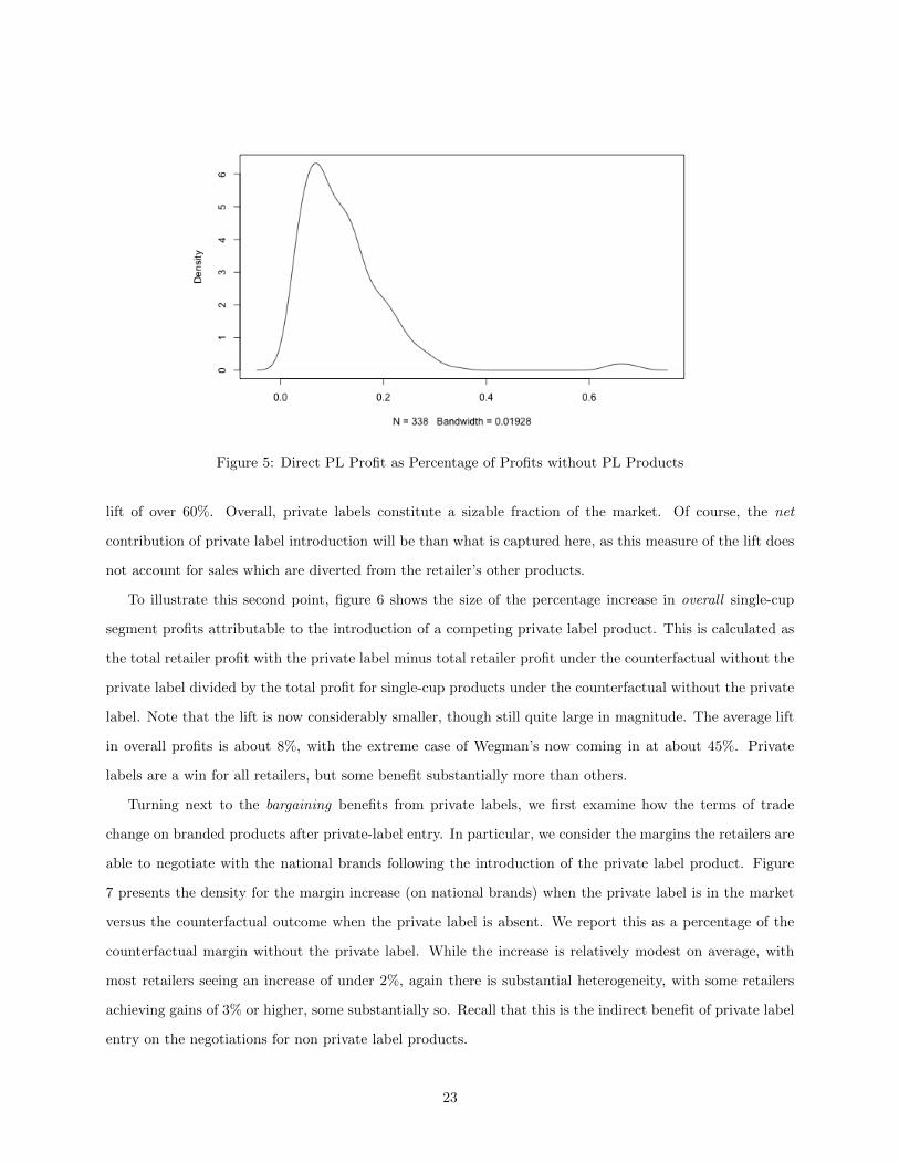
Figure 5: Direct PL Profit as Percentage of Profits without PL Products

lift of over 60%. Overall, private labels constitute a sizable fraction of the market. Of course, the net

contribution of private label introduction will be than what is captured here, as this measure of the lift does

not account for sales which are diverted from the retailer’s other products.

To illustrate this second point, figure 6 shows the size of the percentage increase in overall single-cup

segment profits attributable to the introduction of a competing private label product. This is calculated as

the total retailer profit with the private label minus total retailer profit under the counterfactual without the

private label divided by the total profit for single-cup products under the counterfactual without the private

label. Note that the lift is now considerably smaller, though still quite large in magnitude. The average lift

in overall profits is about 8%, with the extreme case of Wegman’s now coming in at about 45%. Private

labels are a win for all retailers, but some benefit substantially more than others.

Turning next to the bargaining benefits from private labels, we first examine how the terms of trade

change on branded products after private-label entry. In particular, we consider the margins the retailers are

able to negotiate with the national brands following the introduction of the private label product. Figure

7 presents the density for the margin increase (on national brands) when the private label is in the market

versus the counterfactual outcome when the private label is absent. We report this as a percentage of the

counterfactual margin without the private label. While the increase is relatively modest on average, with

most retailers seeing an increase of under 2%, again there is substantial heterogeneity, with some retailers

achieving gains of 3% or higher, some substantially so. Recall that this is the indirect benefit of private label

entry on the negotiations for non private label products.

23

Figure 6: Percentage Increase in Overall Segment Profit Due to PL Entry

Of course, introducing a private label product cannibalizes sales of these same national brands, which

has an offsetting effect on overall profits. Our final set of computations aim to decompose the overall effect

into its constituent parts: the portion arising from competitive stealing (a loss) and the portion arising from

bargaining benefits. In particular, the bargaining benefit is measured as

∑Jrt−PL

((pPLj − wPLj

)−(p−PLj − w−PLj

))s−PLj (15)

while the competitive stealing effect is measured as

∑Jrt−PL

(sPLj − s−PLj

) (pPLj − wPLj

)(16)

Note that the competitive stealing is negative, whereas the bargaining benefit is positive. We present

the distributions of these quantities as a percent of the counterfactual (no private label) single-cup profits

in figures 8 and 9 respectively. Focusing first on figure 8, we note that the bargaining benefit is quite

heterogenous. Most firms derivate a benefit (due to better margins on branded products) that is on the order

of 2% of single-cup segment profits, some firms do substantially better than this (due to the strength of their

private label’s positioning in the marketplace). Figure 9 reveals the offsetting loss due to cannibalization of

sales of branded products. Note that the percentage is larger here (on the order of 6% on average), with

seeing greater than 10% drops in branded profits (recall that these losses are more than offset by the direct

24

Figure 7: Percentage Increase in Margin on National Brands

private label sales that these consumers are diverted to). Finally, figure 10 reveals the magnitude of the

bargaining benefits as percentage of the overall profit increase (i.e. direct profits less cannibalization plus

the increase in margin). We find that the bargaining benefit is quite large, amounting to 20% of the overall

lift on average. Again, there is significant heterogeneity around the mean. The next set of exercises will

explore the source of this heterogeneity, connecting it directly to the strength of the private label programs

in place at the existing retailers.

6 Conclusion

We examine the role of private labels in determining bargaining outcomes in the brew-at-home coffee category.

We exploit a natural experiment in which private label entry was prevented by patent protection, to reveal

how firms behave in the absence of private label competition and how their strategies adapt when entry

occurs. We find that bargaining outcomes are driven primarily by bargaining leverage, while bargaining

ability is relatively symmetric. Moreover, the impact of bargaining leverage is substantial: bargaining

benefits account for roughly 20% of the overall benefit of private label introduction, which is itself on the

order of 10% of pre-introduction profits. Ongoing work is focused on exploring the heterogeneity in these

outcomes.

Note that we have abstracted away from competition between rival retailers. Extending the analysis

to include these effects is the subject of future research. Future work could also consider how lump-sum

25

Figure 8: Bargaining Benefit as Percentage of Profit without PL

transfers (e.g. slotting allowances and other non-linear contracts) or alternative vertical arrangements (e.g.

non-cooperative vertical games) would change the analysis.

26

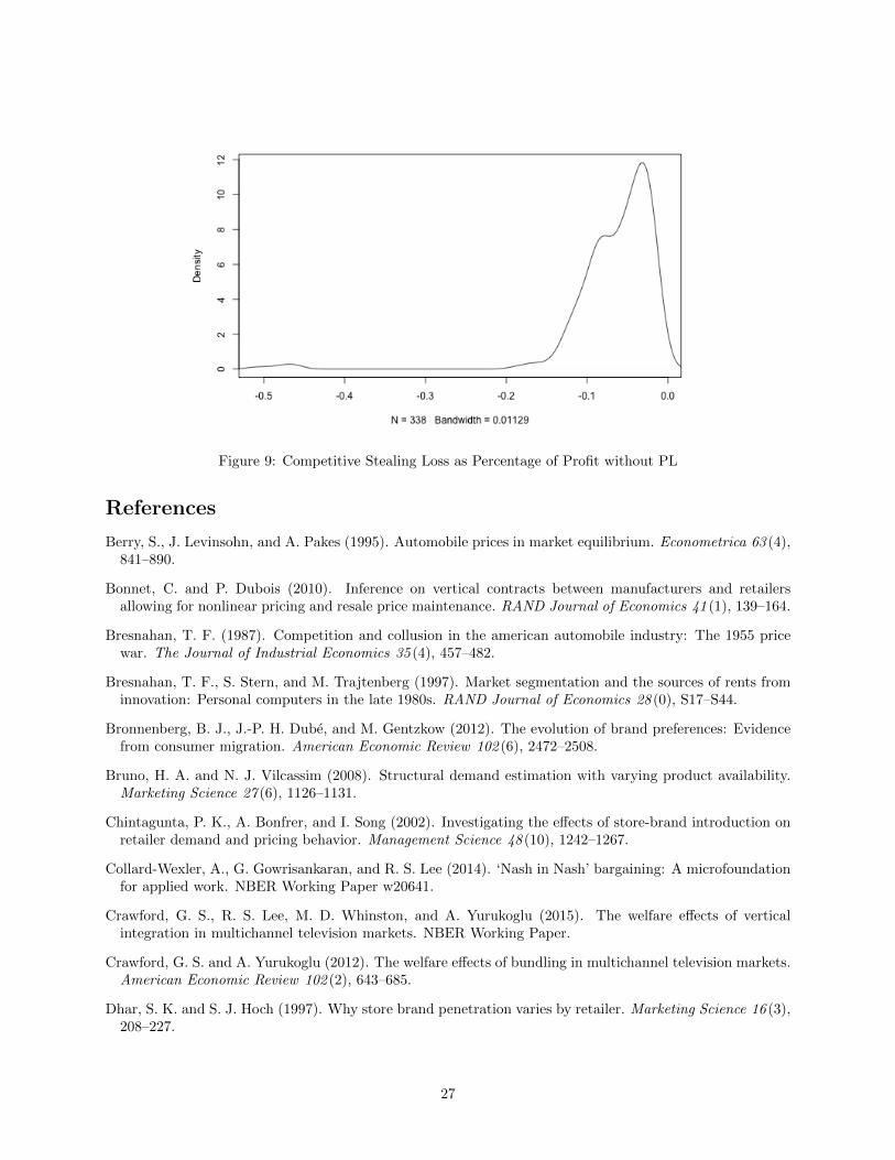
Figure 9: Competitive Stealing Loss as Percentage of Profit without PL

References

Berry, S., J. Levinsohn, and A. Pakes (1995). Automobile prices in market equilibrium. Econometrica 63 (4),841–890.

Bonnet, C. and P. Dubois (2010). Inference on vertical contracts between manufacturers and retailersallowing for nonlinear pricing and resale price maintenance. RAND Journal of Economics 41 (1), 139–164.

Bresnahan, T. F. (1987). Competition and collusion in the american automobile industry: The 1955 pricewar. The Journal of Industrial Economics 35 (4), 457–482.

Bresnahan, T. F., S. Stern, and M. Trajtenberg (1997). Market segmentation and the sources of rents frominnovation: Personal computers in the late 1980s. RAND Journal of Economics 28 (0), S17–S44.

Bronnenberg, B. J., J.-P. H. Dube, and M. Gentzkow (2012). The evolution of brand preferences: Evidencefrom consumer migration. American Economic Review 102 (6), 2472–2508.

Bruno, H. A. and N. J. Vilcassim (2008). Structural demand estimation with varying product availability.Marketing Science 27 (6), 1126–1131.

Chintagunta, P. K., A. Bonfrer, and I. Song (2002). Investigating the effects of store-brand introduction onretailer demand and pricing behavior. Management Science 48 (10), 1242–1267.

Collard-Wexler, A., G. Gowrisankaran, and R. S. Lee (2014). ‘Nash in Nash’ bargaining: A microfoundationfor applied work. NBER Working Paper w20641.

Crawford, G. S., R. S. Lee, M. D. Whinston, and A. Yurukoglu (2015). The welfare effects of verticalintegration in multichannel television markets. NBER Working Paper.

Crawford, G. S. and A. Yurukoglu (2012). The welfare effects of bundling in multichannel television markets.American Economic Review 102 (2), 643–685.

Dhar, S. K. and S. J. Hoch (1997). Why store brand penetration varies by retailer. Marketing Science 16 (3),208–227.

27

Figure 10: Bargaining Benefits as Percentage of Profit Increase

Draganska, M., D. Klapper, and S. B. Villas-Boas (2010). A larger slice or a larger pie? An empiricalinvestigation of bargaining power in the distribution channel. Marketing Science 29 (1), 57–74.

Gandhi, A. and J. Houde (2015). Measuring substitution patterns in differentiated products industries: Themissing instruments. Working Paper (University of Pennsylvania).

Goldfarb, A., Q. Lu, and S. Moorthy (2009). Measuring brand value in an equilibrium framework. MarketingScience 28 (1), 69–86.

Gowrisankaran, G., A. Nevo, and R. Town (2014). Mergers when prices are negotiated: Evidence from thehospital industry. American Economic Review 105 (1), 172–203.

Grennan, M. (2013). Price discrimination and bargaining: Empirical evidence from medical devices. Amer-ican Economic Review 103 (1), 145–177.

Hansen, K., V. Singh, and P. Chintagunta (2006). Understanding store-brand purchase behavior acrosscategories. Marketing Science 25 (1), 75–90.

Ho, K. (2009). Insurer-provider networks in the medical care market. American Economic Review 99 (1),393–430.

Ho, K. and R. S. Lee (2013). Insurer competition in health care markets. NBER Working Paper.

Hoch, S. J. and S. Banerji (1993). When do private labels succeed? Sloan management review 34 (4), 57–67.

Horn, H. and A. Wolinsky (1988). Bilateral monopolies and incentives for merger. RAND Journal ofEconomics 19 (3), 408–419.

Judd, K. L. (1998). Numerical methods in economics. Cambridge, MA: MIT press.

Leibtag, E., A. O. Nakamura, E. Nakamura, and D. Zerom (2007). Cost pass-through in the US coffeeindustry. USDA-ERS Economic Research Report (38), 1–22.

McShane, B. B., C. Chen, E. T. Anderson, and D. I. Simester (2016). Decision stages and asymmetries inregular retail price pass-through. Marketing Science, Forthcoming.

28

Meza, S. and K. Sudhir (2010). Do private labels increase retailer bargaining power? Quantitative Marketingand Economics 8 (3), 333–363.

Misra, S. and S. K. Mohanty (2006). Estimating bargaining games in distribution channels. Working Paper(University of Rochester).

Nash, J. F. (1950). The bargaining problem. Econometrica 18 (2), 155–162.

Nevo, A. (2000a). Mergers with differentiated products: The case of the ready-to-eat cereal industry. RANDJournal of Economics 31 (3), 395–421.

Nevo, A. (2000b). A practitioner’s guide to estimation of random-coefficients logit models of demand. Journalof Economics & Management Strategy 9 (4), 513–548.

Nevo, A. (2001). Measuring market power in the ready-to-eat cereal industry. Econometrica 69 (2), 307–342.

Nielsen Global Survey (2012). The State of private label around the world. The Nielsen Company.

Nijs, V., K. Misra, E. T. Anderson, K. Hansen, and L. Krishnamurthi (2010). Channel pass-through of tradepromotions. Marketing Science 29 (2), 250–267.

Nijs, V. R., K. Misra, and K. Hansen (2013). Outsourcing retail pricing to a category captain: The role ofinformation firewalls. Marketing Science 33 (1), 66–81.

Noton, C. and A. Elberg (2016). Are supermarkets squeezing small suppliers? Evidence from negotiatedwholesale prices. Working Paper (University of Chile).

O’Brien, D. P. and G. Shaffer (2005). Bargaining, bundling, and clout: The portfolio effects of horizontalmergers. RAND Journal of Economics 36 (3), 573–595.

Pauwels, K. and S. Srinivasan (2004). Who benefits from store brand entry? Marketing Science 23 (3),364–390.

Rubinstein, A. (1982). Perfect equilibrium in a bargaining model. Econometrica 50 (1), 97–109.

Sayman, S., S. J. Hoch, and J. S. Raju (2002). Positioning of store brands. Marketing Science 21 (4),378–397.

Schultz, H. (2012). Private labels sales hit $98 billion on 6% growth, report says. Food Navigator USA.

Scott Morton, F. and F. Zettelmeyer (2004). The strategic positioning of store brands in retailer–manufacturer negotiations. Review of Industrial Organization 24 (2), 161–194.

Tenn, S. and J. M. Yun (2008). Biases in demand analysis due to variation in retail distribution. InternationalJournal of Industrial Organization 26 (4), 984–997.

Villas-Boas, S. B. (2007). Vertical relationships between manufacturers and retailers: Inference with limiteddata. Review of Economic Studies 74 (2), 625–652.

Werden, G. J. and L. M. Froeb (1994). The effects of mergers in differentiated products industries: Logitdemand and merger policy. Journal of Law, Economics, & Organization 10 (2), 407–426.

29

A Installed Base Imputation

In this paper we use the single cup category penetration rate (percent households ever purchased in a year)as a proxy for Keurig installed base of retailer shoppers. The point-of-sale data starts from 2008 yet thepenetration rate data are only available starting from 2011.12 In order to obtain installed base prior to 2011,we fit a bass diffusion curve for each individual RMA with initial year being 2004, in which the first Keurigat-home single cup brewer was introduced. The bass diffusion process is given by the following equation,and is estimated using nonlinear least squares for each RMA.

IBjt = mj ∗1− exp (−(pj + qj) ∗ (t− t0))

1 +qjpj

exp (−(pj + qj) ∗ (t− t0))(17)

where j represents retailers, t represents year, and t0 = 2004. We then use the fitted value as the end ofyear installed base throughout the sample to smooth out noises from the penetration rate data. In addition,recognizing that the penetration rate likely captures a subset of the actual Keurig owners among the retailershoppers (namely, leaving out those who own a Keurig but never buy single cup from that retailer), weincrease the fitted value by three percentage points.13 Finally, we interpolate the end of year installed baseto end of quarter ones by assigning 13%, 14%, 25%, and 48% increment to each calendar quarter respectivelybased on Keurig’s quarterly national sales reported in Keurig Green Mountain 2013 10Q. Weekly installedbase levels are interpolated linearly from these quarterly levels.

B Additional Calculations

For simplicity, we drop the krt subscripts and letting wf and cf represent the vector of wholesale pricesand marginal costs for brands owned by manufacturer f . To accommodate the partner revenue sharing wedevelop the notation µ1j and µ2j . We let µ1j to be 1 − κ for the profits for partner brands, κ for Keurigprofits, and 1 otherwise. We let µ2j to be 0 for Keurig profits and 1 otherwise. With this notation, themanufacturer profits in matrix notation are∑

j∈frt

(wjµ1j − cjµ2j) sJrtj (p) (18)

We denote the vector of µ1j containing all terms relevant for manufacturer f to be µf1 and likewise for

µf2 . The derivatives in terms of the wholesale price are then

dF

dwk=

∑j∈f

(wjµ1j − cjµ2j)dsjdwk

+ skµ1k (19)

=(wf · µf1 − cf · µ

f2

)′ dsdwk

+ skµ1k (20)

dR

dwk=

∑j∈J

((pj − wj)

dsjdwk

+dpjdwk

sj

)− sk (21)

= (p− w)′ ds

dwk+

(dp

dwk

)′s− sk. (22)

(23)

We now consider the calculation of the two total derivatives contained in these expressions,dsjdwk

anddpjdwk

.

12Some RMA-years had too few buyers in the IRI panel data to make a projection to the shopper population for that specificRMA-year of the percentage of shoppers that buy any single-cup products. We use the fitted values of a multiple regressionto impute the missing values, where the regression includes independent variables the (raw, not projected) observed numberof buyers divided by the raw number of shoppers, the share of the K-cup sales out of coffee sales, total K-cup and total coffeesales, average dollar sales weighted ACV for K-cup products, the average, minimum, and maximum number of K-cup brands(and polynomials of these), and a cubic function of the year dummies interacted with the coffee penetration rate.

13We determined the 3% value by analyzing the category share out of total coffee to infer a lower bound of the installed base.

30

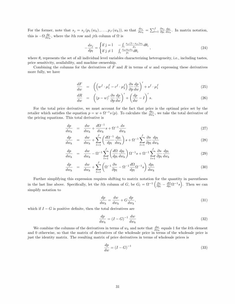
For the former, note that sj = sj (p1 (wk) , . . . , pJ (wk)), so thatdsjdwk

=∑Jl=1

∂sj∂pl

dpldwk

. In matrix notation,

this is −Ω dpdwk

, where the lth row and jth column of Ω is

−dsjdpl

=

if j = l −

∫isji(1−sji)αi

pjdθi

if j 6= l∫isjisliαi

pldθi

, (24)

where θi represents the set of all individual level variables characterizing heterogeneity, i.e., including tastes,price sensitivity, availability, and machine ownership.

Combining the columns for the derivatives of F and R in terms of w and expressing these derivativesmore fully, we have

dF

dw=

((wf · µf1 − cf · µ

f2

) ∂s∂p

dp

dw

)′+ sf · µf1 (25)

dR

dw=

((p− w)

′ ∂s

∂p

dp

dw

)′+

(dp

dw− I)′s. (26)

For the total price derivative, we must account for the fact that price is the optimal price set by theretailer which satisfies the equation p = w + Ω−1s (p). To calculate the

dpjdwk

, we take the total derivative ofthe pricing equations. This total derivative is

dp

dwk=

dw

dwk+dΩ−1

dwks+ Ω−1 ds

dwk(27)

dp

dwk=

dw

dwk+

J∑l=1

(dΩ−1

dpl

dpldwk

)s+ Ω−1

J∑l=1

∂s

∂pl

dpldwk

(28)

dp

dwk=

dw

dwk− Ω−1

J∑l=1

(dΩ

dpl

dpldwk

)Ω−1s+ Ω−1

J∑l=1

∂s

∂pl

dpldwk

(29)

dp

dwk=

dw

dwk+

J∑l=1

(Ω−1 ∂s

∂pl− Ω−1 dΩ

dplΩ−1s

)dpldwk

(30)

Further simplifying this expression requires shifting to matrix notation for the quantity in parentheses

in the last line above. Specifically, let the lth column of G, be Gl = Ω−1(∂s∂pl− dΩ

dplΩ−1s

). Then we can

simplify notation to

dp

dwk=

dw

dwk+G

dp

dwk, (31)

which if I −G is positive definite, then the total derivatives are

dp

dwk= (I −G)

−1 dw

dwk(32)

We combine the columns of the derivatives in terms of wk and note that dwdwk

equals 1 for the kth elementand 0 otherwise, so that the matrix of derivatives of the wholesale price in terms of the wholesale price isjust the identity matrix. The resulting matrix of price derivatives in terms of wholesale prices is

dp

dw= (I −G)

−1(33)

31

Finally, letting Ωjh be the element in the jth row and hth column, the ∂Ω/∂pl derivatives are defined by

∂Ωjh∂pl

=

if l = h = j −∫isli(1−sli)αi((1−2sli)αi−1)

p2ldθi

if l = j 6= h∫islishiαi((1−2sli)αi−1)

p2ldθi

if l = h 6= j∫islisji(1−2sli)α

2i

pjpldθi

if l 6= h = j∫islisji(1−2sji)α

2i

pjpldθi

if l 6= h 6= j −2∫isjislishiα

2i

pjpldθi

(34)

B.1 Approximating wjt for counterfactual PL manufacturers

In most cases, the Retailer’s disagreement payoffs as defined in section 3.2.2 are mostly the counterfactualprofits without the presence of the brand that is bargained over. However, for the private label bargains thedisagreement payoffs can involve counterfactual payoffs for an alternative manufacturer. Unlike in the mainsupply-side estimation, here we can’t recover wholesale prices from observed prices, since the price is notobserved for the counterfactual private label brand. Yet we need the wholesale price of the counterfactualprivate label brand in order to determine the prices and shares necessary to construct the disagreementpayoff.

Intuitively, what this disagreement payoff represents the beliefs or expectations of the retailer aboutprofits if the bargain fails. We approximate these beliefs via a parametric policy function conditioningon the states. Specifically, we approximate the percentage discount from the Keurig wholesale price as afunction of the type of actual private label manufacturer (with Keurig vs. with non-Keurig manufacturer),the number of single-cup competing brands, the presence of Eight O’Clock single-cup, and the retail pricedifference between Keurig and the actual private label brand. The relationship type captures potentialdifferences in the product quality and manufacturing costs of the two types of manufacturers. The numberof brands is aimed at focusing on the degree of competition and saturation of the market. The presence ofEight O’Clock captures the presences of the closest national brand competitor to the private label in pricespace. The retail price difference captures the relative quality of the private label in that retailer.

We estimate this parametric policy function using the observed data and project to the counterfactualcases during estimation.

B.2 Standard Errors

Current standard errors are calculated assuming homoskedastic errors under the non-linear 2SLS (Camererand Trivedi 2005). The formula is

V(β)

= s2(D′Z(Z ′Z)−1Z ′D

)−1

, (35)

where s2 is the consistent estimate of the variance of the (logged) residuals and D is the matrix derivativesof the (logged) residual in terms of the parameters. These derivatives are characterized by

∂ (φrkt (θc)− φrk)

∂φrk= −1rk (36)

∂ (φrkt (θc)− φrk)

∂θc= − Rk

∂Rk

∂wkFk

(∂ ∂Fk

∂wk

∂θc−

∂Fk

∂wk

∂Fk

∂θc

Fk

)(37)

∂Fk∂θc

= X′

c,f (sf−k − sf ) · µf2 (38)

∂ ∂Fk

∂wk

∂θc= −X

′

c,f

dsfdwk

· µf2 , (39)

and where the remaining quantities are defined in the main text.

32

We note that whereas for obtaining the point estimates we concentrate out the parameters φrk for thestandard errors, we reincorporate the appropriate dummy variables as instruments. This allows estimationof the standard errors for those values as well.

B.3 Gradient for optimization

The gradient is passed to the optimizer during optimization. The gradient that is used is

∆Qn (θ) = 2u′Z(Z ′Z)−1Z ′D, (40)

where u is the vector of logged residuals, D is the matrix of derivatives of the (logged) residuals in terms of theparameters excluding the bargaining parameters. We note here that because we use the within transformationto simplify the non-linear optimization, the D does not include the derivatives in terms of φrk. Likewise, theinstrument matrix, Z, does not include the corresponding within transformation instruments. However, theformulas for the derivatives in terms of the cost parameters are still denoted as above in the section B.2.

B.4 Jacobian of the constraint for constrained optimization

For the optimization, we need to ensure that the costs, c, margins, manufacturer’s difference between theagreement and disagreement payoff (i.e., Fk), and the ratio of βs (i.e., φ) are all positive. This imposes a setof inequality constraints that must be satisfied for the estimation to reach a parameter vector that is feasibleunder the structural model.

During the constrained optimization routine, we calculate the Jacobian of the constraints, which is astacked matrix of derivatives with number of rows equal to the total number of constraints and numberof columns equal to the number of cost parameters in θc. The derivatives for Fk and φ are presented inequations (38) and (37) above. The remaining calculations are presented below, noting that this is for asingle manufacturer:

∂c (θ)

∂θm= Xc,m, for all µ2j > 0 (41)

∂ (wµ1 − c (θ)µ2)

∂θm= −Xc,mµ2 (42)

B.5 Counterfactuals and simulating data

The counterfactuals rely on our ability to simulate data from the bargaining problem. We do so withknowledge of the parameters of the demand and supply side model as well as knowledge of the predeterminedvariables in the model. Our main task is to calculate the w and p vectors for each period and market.

The optimal p vector can be calculated for any given w by successive approximation on the price firstorder conditions, p = w+Ω (p)

−1s (p). With the monopolist retailer assumptions, these conditions represent

a unique equilibrium.Our counterfactuals are calculated by proposing the set of products in the bargaining setting and then

guessing at the wholesale price, w, and solving for p. With these quantities in hand, we use the firstorder conditions of the bargaining problem to solve for the w via successive approximation. The successiveapproximation takes the following form:

wh+1 = cµ2

µ1−s(wh)

+ V(wh)

Ψ (wh) · µ1, (43)

where h indexes the iterations, w, c, and s are the respective Jx1 vectors of wholesale prices, costs, andshares, V is a Jx1 vector that represents the internalization of the profit impact of this bargain on otherproducts the manufacturer controls, and Ψ is Jx1 vector related to a ”mark-up” term. The jth element ofΨ is

Ψ(j) =dsjdwj

+ ρjsj , (44)

33

where ρj is defined by

ρj =βj

1− βj

dRj

dwj

Rj, (45)

and the diagonal matrix with ρj on the (j, j)th element is ρ. V is defined by

V =

(M ∗ (1− I) ∗

(ds

dw+ ρs

))· (w · µ1 − c · µ2) , (46)

where s is a JxJ matrix with the (j, k) element containing the difference between the share of product kwith all products versus the share without product j, where the retail prices are set optimally given thewholesale price and the set of products in the market. The matrices M ∗ (1− I) are element-wise multipliedand represent the ownership structure with the diagonal elements containing zeros.

The derivation of equation (43) relies on separating the jth (bargained) product from dFj/dwj and Fj ,moving that to the lefthand side and separating wj from the other terms.

We note that we have no proof that the bargaining problem has a unique equilibrium. We try multiplestarting points in order to evaluate whether multiple equilibria are obtained.

34