Pricing and Trading European Options by Combining

Artificial Neural Networks and Parametric Models with

Implied Parameters

Citation for published item:

Andreou, P. C., Charalambous, C., Martzoukos, S. H. (2008). Pricing and

trading European options by combining artificial neural networks and

parametric models with implied parameters. European Journal of Operational

Research 185, 1415-1433.

View online & further information on publisher’s website:

http://dx.doi.org/10.1016/j.ejor.2005.03.081

Pricing and Trading European Options by Combining Artificial Neural Networks

and Parametric Models with Implied Parameters

Panayiotis C. Andreou1, Chris Charalambous2, and Spiros H. Martzoukos*3

University of Cyprus – Department of Public and Business Administration

This version: March 2005

Keywords: Finance, neural networks, empirical option pricing Acknowledgements: This work has been partly funded by the Hermes European Center of Excellence in Computational Finance and Economics, and a University of Cyprus grant for research in ANNs and Derivatives. We are thankful to Paul Lajbcygier for comments and discussions. We appreciate comments on earlier drafts by participants at the 9th Annual Conference of the Multinational Finance Society (Paphos, July 2002), the International Conference of Artificial Neural Networks (Madrid, August 2002), the International Workshop on Computational Management Science (Limassol, March 2003), the joint EURO/INFORMS Meeting (Istanbul, July 2003), the European Union Workshop series on Mathematical Optimization Models for Financial Institutions (Ayia Nappa, November 2003), and the FMA International/Europe Conference (Zurich, June 2004). 1,2,3 PhD Candidate, Professor of Management Science, and Assistant Professor of Finance respectively * Corresponding author: Spiros H. Martzoukos, Assistant Professor of Finance University of Cyprus, Department of Public and Business Administration P.O. Box 20537, CY 1678 Nicosia – Cyprus Fax: +357-22 89 24 60, Tel.: +357-22 89 24 74 email: baspiros@ucy.ac.cy

1

Pricing and Trading European Options by Combining

Artificial Neural Networks and Parametric Models with Implied Parameters

Abstract

We compare the ability of the parametric Black and Scholes, Corrado and Su models, and Artificial Neural Networks to price European call options on the S&P 500 using daily data for the period January 1998 to August 2001. We use several historical and implied parameter measures. Beyond the standard neural networks, in our analysis we include hybrid networks that incorporate information from the parametric models. Our results are significant and differ from previous literature. We show that the Black and Scholes based hybrid artificial neural network models outperform the standard neural networks and the parametric ones. We also investigate the economic significance of the best models using trading strategies (extended with the Chen and Johnson modified hedging approach). We find that there exist profitable opportunities even in the presence of transaction costs.

2

1. Introduction

In this paper we compare parametric option pricing models (OPMs) -- Black

and Scholes (1973) (BS) and the semi-parametric Corrado and Su (1996) (CS) -- with

several artificial neural network (ANN) configurations. We compare them with respect

to pricing the S&P 500 European call options, and trading strategies are

implemented in the presence of transaction costs.

Black and Scholes introduced in 1973 their milestone OPM. Despite the fact

that BS and its variants are considered as the most prominent achievements in

financial theory in the last three decades, empirical research has shown that the

formula suffers from systematic biases (see Black and Scholes, 1975, MacBeth and

Merville, 1980, Gultekin et al., 1982, Rubinstein, 1985, Bates, 1991 and 2003,

Bakshi et al., 1997, Andersen et al., 2002, and Cont and Fonseca, 2002). The BS

bias stems from the fact that the model has been developed under a set of simplified

assumptions such as geometric Brownian motion of stock price movements,

constant variance of the underlying returns, continuous trading on the underlying

asset, constant interest rates, etc.

Post-BS research (e.g. stochastic volatility, jump-diffusion, stochastic interest

rates, etc.) has not managed to either generalize all the assumptions of BS or provide

results truly consistent with the observed market data. These models are often too

complex to implement, have poor out-of-sample pricing performance and have

implausible and sometimes inconsistent implied parameters (see Bakshi et al.,

1997). This justifies the severe time endurance of BS1. Together with the BS model,

we also consider the semi-parametric CS model that allows for excess skewness and

kurtosis, as a model that can proxy for other more complex parametric ones.

Nonparametric techniques such as Artificial Neural Networks are promising

alternatives to the parametric OPMs. ANNs do not necessarily involve directly any

financial theory because the option’s price is estimated inductively using historical

or implied input variables and option transactions data. Option-pricing functions are

multivariate and highly nonlinear, so ANNs are desirable approximators of the

empirical option pricing function. Parametric models describe a stationary nonlinear

relationship between a theoretical option price and various variables. Since it is

known that market participants change their option pricing attitudes from time to

time (i.e. Rubinstein, 1985) a stationary model may fail to adjust to such rapidly

changing market behavior (see also Cont and Fonseca, 2002, for evidence of

noticeable variation in daily implied parameters). ANNs if frequently trained can

1 According to Andersen et al., (2002), “the option pricing formula associated with the Black and Scholes diffusion is routinely used to price European options, although it is known to produce systematic biases”.

3

adapt to changing market conditions, and can potentially correct the aforementioned

BS bias (Hutchison et al., 1994, Lajbcygier et al., 1996, Garcia and Gencay, 2000,

Yao and Tan, 2000).

Beyond the standard ANN target function we further examine the hybrid ANN

target function suggested by Watson and Gupta (1996) and used for pricing options

with ANNs in Lajbcygier et al. (1997). In the hybrid models the target function is the

residual between the actual call market price and the parametric option price

estimate. In previous studies the standard steepest descent backpropagation

algorithm is (mostly) used for training the feedforward ANNs. It is shown in

Charalambous (1992) that this learning algorithm is often unable to converge rapidly

to the optimal solution. Here we utilize the modified Levenberg-Marquardt (LM) algorithm which is much more sophisticated and efficient in terms of time capacity

and accuracy (Hagan and Menhaj, 1994). In contrast to most previous studies,

thorough cross-validation allows us to use a different network configuration in

different testing periods.

The data for this research come from two dominant world markets, the New

York Stock Exchange (NYSE) for the S&P 500 equity index and the Chicago Board of

Options Exchange (CBOE) for call option contracts, spanning a period from January

1998 to August 2001. To our knowledge, the resulting dataset is larger than the ones

used in other published studies. We also (similarly to Rubinstein, 1985, Bates, 1996,

Bakshi et al., 1997; see discussion in Bates, 2003) reserve option datapoints that in

several ANN studies were dropped out of the analysis. Note that in order to check the

robustness of the results we repeated the analysis using a reduced dataset following

Hutchison et al. (1994). We examine more explanatory variables including historical,

weighted average implied and pure implied parameters. Also, instead of constant

maturity riskless interest rate, we use nonlinear interpolation for extracting a

continuous rate according to each option’s time to maturity.

Lastly, although previous researchers have exploited BS or ANNs, little has

been reported for the case of CS2 and nothing for the hybrid ANNs that use

information derived by CS. To investigate the economic significance of the alternative

option pricing approaches, trading strategies without and with the inclusion of

transaction costs are utilized. These trading strategies are implemented with the

standard delta-hedging values implied by each model, but also with the corrected

values according to the (widely neglected) Chen and Johnson (1985) methodology.

In the following we first review the BS and CS models, and the standard and

hybrid ANN model configuration. Then we discuss the dataset, the historical and

2 An exception is the paper by Sami Vahamaa (2003) that examined the hedging performance of the CS model without including transaction costs.

4

implied parameter estimates we derive, and we define the parametric and ANN

models according to the parameters used. Subsequently we review the numerical

results with respect to the in- and out-of-sample pricing errors; and we discuss the

economic significance of dynamic trading strategies both in the absence and in the

presence of transaction costs. The final section concludes. In general, our results

are novel and significant. We identify the best hybrid ANN models, and we provide

evidence that (even in the presence of transaction costs), profitable trading

opportunities still exist.

2. Option pricing: BS, CS and ANNs

2.1. The parametric models

The Black Scholes formula for European call options modified for dividend-

paying underlying asset is:

1 2( ) ( )BS T rTc Se N d Xe N dδ− −= − , (1)

where,

- 2

1ln( / ) ( ) ( ) /2S X r T Td δ σ

σ+ +

=Τ

, (1.a)

and

2 1d d Tσ= − . (1.b)

BSc ≡premium paid for the European call option; S ≡ spot price of the underlying asset;

X ≡ exercise price of the option; r ≡ continuously compounded riskless interest rate;

δ ≡ continuous dividend yield paid by the underlying asset; T ≡ time left until the

option expiration; 2σ ≡yearly variance rate of return for the underlying asset; (.)N ≡ the

standard normal cumulative distribution.

The standard deviation of continuous returns (σ) is the only variable in

Equations 1.a and 1.b that cannot be directly observed in the market. For this study,

we use both historical and implied volatility forecasts. For the Historical Volatility we

use the past 60 days. The Implied Volatility (IVL) calculation involves solving

Equation 1 iteratively for σ given the values of the observable mrkc (the most

recently observed market price of a call option), and the relevant values of S, X, T, r and δ . Contrary to historical volatility, IVL has desirable properties that make it

5

attractive to practitioners: it is forward looking, and avoids the assumption that past

volatility will be repeated.

If BS is a well-specified model, then all IVLs on the same underlying asset

should be the same, or at least deterministic functions of time. Unfortunately, many

researchers have reported systematic biases. For example, Rubinstein (1985) has

shown that IVL derived via BS as a function of the moneyness ratio (S/X) and time to

expiration (T) often exhibits a U shape, the well known volatility smile. Bakshi et al.

(1997) report that implicit stock returns’ distributions are negatively skewed with

more excess kurtosis than allowable in the BS lognormal distribution. This is why we

usually refer to BS as being a misspecified model with an inherent source of bias

(see also Latane and Rendleman, 1976, Bates, 1991, Canica and Figlewski, 1993,

Bakshi et al., 2000, and Andersen et al., 2002). For the aforementioned reason we

include in our analysis the Corrado and Su (1996) (see also the correction in Brown

and Robinson, 2002) model that explicitly allows for excess skewness and kurtosis.

The CS model is a semi-parametric model since it does not rely on specific

assumptions about the underlying stochastic process. Corrado and Su define their

model as:

3 3 4 4( 3)CS BSc c Q Qμ μ= + + − , (2)

23 1 1 1

1 ((2 ) ( ) ( ))3!

TQ Se T T d n d T dδ σ σ σ−= − − Ν , (2.a)

2 3 3/24 1 1 1 1

1 (( 1 3 ( )) ( ) ( ))4!

TQ Se T d T d T n d T N dδ σ σ σ σ−= − − − + , (2.b)

)2/exp(21)( 2zπ

zn −= , (2.c)

where cBS is the BS value for the European call option adjusted for dividends, and 3μ

and 4μ are the coefficients of skewness and kurtosis of the returns.

2.2. Neural networks

A Neural Network is a collection of interconnected simple processing elements

structured in successive layers and can be depicted as a network of

arcs/connections and nodes/neurons. Fig. 1 depicts a fully-connected ANN

architecture similar to the one applied in this study. This network has three layers:

an input layer with N input variables, a hidden layer with H neurons, and a single

6

neuron output layer. Each connection is associated with a weight, kiw , and a bias,

kb , in the hidden layer and a weight, kv , and a bias, 0v , for the output layer (k =

1,2,…,H, i = 1,2,…,N). A particular neuron node is composed of: i) the vector of input signals, ii) the vector weights and the associated bias, iii) the neuron itself that sums

the product of the input signal with the corresponding weights and bias, and finally,

iv) the neuron transfer function. In addition, the outputs of the hidden layer

( (1) (1) (1)1 2, ... Hy y y ) are the inputs for the output layer. Since we want to approximate the

market options pricing function, ANNs operate as a non-linear regression tool:

( ) ANNY G x ε= +% , (3)

that maps the unknown relation, G(.), between the input variable vector,

1 2[ , ,..., ]Nx x x x=% , the target function, Y , and the error term, ANNε . Inputs are set up

in feature vectors, 1 2[ , ..., ]q q q Nqx x x x=% for which there is an associated and known

target, qY t≡ (in our case, /mrkq q qt c X≡ ), with 1,2,...,q P≡ , where P is the number of

the available sample features. According to Fig. 1, the operation carried out for

estimating output y (in our case, /qANN

q qy c X≡ ), is the following:

0 01 1

[ ( )]H N

k H k ki ik i

y f v v f b w x= =

= + +∑ ∑ . (4)

[Figure 1 here]

For the purpose of this study, the hidden layer always uses the hyperbolic tangent

sigmoid transfer function, while the output layer uses a linear transfer function. In

addition, ANN architectures with only one hidden layer are considered since they

operate as a nonlinear regression tool and can be trained to approximate most

functions arbitrarily well (Cybenko, 1989). High accuracy can be obtained by

including enough processing nodes in the hidden layer.

To train the ANNs, we utilized the modified LM algorithm. According to LM,

the weights and the biases of the network are updated in such a way so as to

minimize the following sum of squares performance function:

2 2 20 0

1 1 1 1 1( ) ( ) ( [ ( )] )

P P P H N

q q q k H k ki iq qq q q k i

F W e y t f v v f b w x t= = = = =

= ≡ − ≡ + + −∑ ∑ ∑ ∑ ∑ , (5)

7

where, W is an n-dimensional column vector containing the weights and biases:

1 11 0[ ,..., , ,..., , ,..., ]TH HN HW b b w w v v= . Then, at each iteration τ of LM, the weights

vector W is updated as follows:

)()(])()([ τττττττ μ WeWJIWJWJWW TT 11

−+ +−= , (6)

where I is an n n identity matrix, ( )J W is the P n Jacobian matrix of the P-

dimensional output error column vector ( )e W , and τμ is like a learning parameter

that is adjusted in each iteration in order to secure convergence. Further technical

details about the implementation of LM can be found in Hagan and Menhaj (1994)

and Hagan et al. (1996). In addition to the standard use of ANNs where /mrkq q qt c X≡ ,

we also try hybrid ANNs in which the target function is the residual between the

actual call market price and the BS or CS call option estimation:

/ /mrk kq q q q qt c X c X≡ − , (7)

with k defining inputs from a parametric model. To avoid neuron saturation, we

scale input variables using the mean-variance transformation (z-score) defined as

follows:

( )/i i i iz x sμ= −% % , (8)

where ix% is the vector containing all of the available observations related to a certain

input/output variable for a specific training period, iμ is the mean and is the

standard deviation of this vector. Moreover, we also utilize the network initialization

technique proposed by Nguyen and Windrow (see Hagan et al., 1996) that generates

initial weights and bias values for a nonlinear transfer function so that the active

regions of the layer’s neurons are distributed roughly evenly over the input space.

In this study for each input variable set of each training sample, all the

available networks having two to ten hidden neurons are cross-validated (in total

nine). Moreover, since the initial network weights affect the final network

performance, for a specific number of hidden neurons the network is initialized,

trained and validated many times. Each network is estimated and optimized using

the Mean Square Error (MSE) criterion shown in Equation 5 for no more than two-

hundred iterations. The dataset is divided into three sub-sets. The first is the

training (estimation) set. The second is the validation set where the ANN model’s error

8

is monitored and the optimal number of hidden neurons and their weights are

defined, via an early stopping procedure (MSE fails to decrease in 10 consecutive

iterations). Given the optimal ANN structure, its pricing capability is tested in a third

separate testing dataset.

3. Data, parameter estimates (historical and implied), and model implementation

Our dataset covers the period January 1998 to August 2001. To our

knowledge, the resulting dataset is larger than the one used in other published

studies and reserves option data points that in most of the previous studies were

dropped out of the analysis. After implementing the filtering rules, our dataset

consists of 76,401 data points, with an average of 35,000 data points per

(overlapping rolling training-validation-testing) sub-period (see Fig. 2). Hutchison et

al. (1994) have an average of 6,246 data points per sub-period. Lajbcygier et al.

(1996) include 3,308 data points, Yao et al. (2000) include 17,790 data points, and

Schittenkopf and Dorffner (2001) include 33,633 data points. The S&P 500 Index call

options are considered because this option market is extremely liquid and one of the

most popular index options traded on the CBOE. This market is the closest to the

theoretical setting of the parametric models. Along with the index, we have collected a daily dividend yield, δ , provided online by Datastream.

3.1. Observed and historically estimated parameters Moneyness Ratio (S/X): The moneyness ratio may explicitly allow the ANNs to

learn the moneyness bias associated with the BS (see also Garcia and Gencay,

2000). The dividend adjusted moneyness ratio ( )/TSe Xδ− is used in this study with

ANNs because it is more informative. The simple moneyness ratio S/X is used in

order to tabulate results as in Hutchison et al. (1994). We adopt the following

terminology: very deep out of the money (VDOTM) when S/X<0.85, deep out the

money (DOTM) when 0.85≤S/X<0.90, out the money (OTM) when 0.90≤S/X<0.95, just

out the money (JOTM) when 0.95≤S/X<0.99, at the money (ATM) when

0.99≤S/X<1.01, just in the money (JITM) when 1.01≤ S/X <1.05, in the money (ITM)

when 1.05≤S/X<1.10, deep in the money (DITM) when 1.10≤S/X<1.35, and very deep

in the money (VDITM) when S/X≥1.35.

Time to maturity (T ): For each option contract, trading days are computed

assuming 252 days in a year. In terms of time length, an option contract is classified

9

as short term maturity when its maturity is less than 60 days, as medium term maturity when its maturity is between 60 and 180 days and as long term maturity when it has maturity longer than (or equal to) 180 days.

Riskless interest rate (r ): Most of the studies use 90-day T-bill rates (or

similar when this is unavailable) as approximation of the interest rate. We use

nonlinear cubic spline interpolation for matching each option contract with a

continuous interest rate, r , that corresponds to the option’s maturity, by utilizing

the 3-month, 6-month and one-year T-bill rates collected from the U.S. Federal

Reserve Bank Statistical Releases. Historical Volatilities (σ ): The 60-day historical volatility is calculated using all

the past 60 log-relative index returns and is symbolized as 60σ .

CBOE VIX Volatility Index: It was developed by CBOE in 1993 and is a

measure of the volatility of the S&P 100 Index3. VIX is calculated by taking the

weighted average of the implied volatilities of eight S&P 100 Index call and put

options with an average time to maturity of 30 days. This volatility measure can only

be used with BS and is symbolized as BSvixσ .

Skewness and Kurtosis: The 60-day skewness ( 3,60CSμ ) and kurtosis ( 4,60

CSμ )

needed for the CS model are approximated from the sixty most recent log-returns of

the S&P 500.

3.2. Implied parameters We adopt the Whaley’s (1982) simultaneous equation procedure to minimize a

price deviation function with respect to the unobserved parameters. As with Bates

(1991), market option prices (cmrk) are assumed to be the corresponding model prices

(ck, k defining input from a parametric model) plus a random additive disturbance

term. For any option set of size Nt (Nt refers to the number of different call option

transaction datapoints available on a specific day), the difference:

kN

mrkN

kN ttt

cc −=ε (9)

between the market and the model value of a certain option is a function of the

values taken by the unknown parameters. To find optimal implied parameter values

we solve an unconstrained optimization problem that has the following form:

3 The S&P 100 Index and S&P 500 Index exhibit 30 day log-return average correlations for the period January 1998 to August 2002 of about 0.98.

10

∑=

=t

k

N

l

kl )(min)t(SSE

1

2εθ

, (10)

where t represents the time instance, and kθ the unknown parameters associated

with a specific parametric OPM ( { }BSθ σ= , 3 4{ , , }CSθ σ μ μ= ). The SSE is minimized via

a non-linear least squares optimization based on the LM algorithm. To minimize the

possibility to obtain implied parameters that correspond to a local minimum of the

error surface (see also Bates, 1991, and Bakshi et al., 1997), with each model we use

three different starting values for the unknown parameters based on reported

average values in Corrado and Su (1996).

A difference of our approach compared to previous studies is that the above

minimization procedure is used daily to derive four different sets of implied

parameters for each parametric model. The first optimization is performed by

including all available options transaction data in a day to obtain daily average

implied structural parameters. Alternatively, for a certain day we minimize the SSE

of Equation 10 by fitting the BS and CS for options that share the same maturity

date as long as four different available call options exist. We thus get daily average

per maturity parameters. In a third step, for every maturity each available option

contract is grouped with its three nearest options in terms of the moneyness ratio in

order to minimize the above SSE function, deriving thus parameters average per the

4 closest contracts; such estimates are ignored in previous research. We finally

calibrate the implied structural parameters, by focusing on the Brownian volatility

for each contract so as to drive the residual error to zero or to a negligible value. In

the case of BS this is quite simple and we can easily obtain a contract specific

volatility estimate. For CS we need three structural parameters, so for each call

option we minimize Equation 10 with respect to the Brownian volatility after fixing

the skewness and kurtosis coefficients to the values obtained from the previous

procedure that gave the average per the 4 closest implied parameters. Two kinds of

constraints are included in the optimization process for practical reasons:

nonnegative implied volatility parameters are obtained by using an exponential

transformation; and the skewness of CS4 is permitted to vary in the range [–10, 5]

whereas kurtosis is constrained to be less than 30. Unlike previous studies, we 4 If not somehow constrained, skewness and kurtosis can take implausible values (i.e. Bates, 1991) due to model overfitting that will lead to enormous pricing errors on the next day (especially for deep in the money options). In our case these constraints were binding in less than 2% of the whole dataset.

11

include contract specific implied parameters since these are widely used by market

practitioners (i.e. Bakshi et al., 1997, pg. 2019).

For notational reasons, implied parameters obtained from the first step are

denoted by the subscript av, from the second step by the subscript avT, from the

third step by the subscript avT4, and from the fourth step by the subscript con. The

four different implied BS volatility estimates are symbolized as: BSjσ ,

},4,,{ conavTavTavj = , whilst the four different sets of CS parameters as:

3, 4,{ , }CS CS CSj j jσ μ μ . For pricing and trading reasons at time instant t, the implied

structural parameters derived at day t-1 are used together with all other needed information (S, T, X, r, and δ ).

It is known that ANN input variables should be presented in a way that

maximizes their information content. When we price options, the parametric OPM

formulas adjust those values to represent the appropriate value that corresponds to

an option’s expiration period. According to this rationale, volatility measures for use

with the ANNs are transformed by multiplying each of the yearly volatility forecast

with the square root of each option’s time to maturity ( j j Tσ σ=% , where j={60, vix,

av, avT, avT4, con}). We denote these volatility measures as BSjσ% and CS

jσ% ; and we

name them as maturity (or expiration) adjusted volatilities. Additionally, for the case

of CS, skewness 3,CSjμ , {60, , , 4, }j av avT avT con= , is transformed by multiplication

with Q3 that represents the marginal effect of nonnormal skewness. Similarly, 4,CSjμ

is multiplied with Q4. We denote these adjusted parameters as 3,CS

jμ% (adjusted

skewness), and 4,CS

jμ% (adjusted kurtosis).

3.3. Output variables, filtering and processing

The BS ( BSqc ) and CS ( CS

qc ) outputs, are used as an estimate for the market

call option, mrkqc . For training ANNs, the call standardized by the striking price,

/mrkq qc X , is used as the target function to be approximated. In addition, we

implement the hybrid structure where the target function represents the pricing

error between the option’s market price and the parametric models estimate,

/ /mrk kq q q qc X c X− .

Before filtering, more than 100,000 observations were included for the period

January 1998 – August 2001. The filtering rules we adopt are: i) eliminate an

12

observation if the call contract price, mrkt,mc , m defining each traded contract, is greater

than the underlying asset value, tS ; ii) exclude an observation if the call moneyness

ratio is larger than unity, St/Xm>1, and the call price, mrkt,mc , is less than its lower

bound, , , , ,m t m t m t m tT r Tt mS e X eδ− −− ; iii) eliminate all the options observations with time to

maturity less than 6 trading days. The latter filtering rule is adopted to avoid extreme

option prices that are observed due to potential illiquidity problems; iv) price quotes lower than 0.5 index points are not included; v) maturities with less than four call option observations are also eliminated, vi) in addition, to remove impact from thin

trading we eliminate observations according to the following rule: eliminate an

observation if the mrkt,mc is equal to mrk

1t,mc − and if the open interest for these days stays

unchanged and if the underlying asset S has changed. [Table 1, here]

Our final dataset consists of 76,401 datapoints. Table 1 exhibits some of the

properties of our sample tabulated according to moneyness ratio and time to

maturity forming 27 different moneyness/maturity classes. We provide the average

values for cmrk and BSconσ , and the number of observations within each moneyness and

maturity class. The implied volatility, BSconσ , presents a non-flat moneyness structure

when fixing the time to maturity and vice versa revealing the bias associated with

BS. Moreover, we should notice that DITM and VDITM options dominate in number

of datapoints all other classes, so unlike studies that ignore these options we choose

to include them in the dataset. For the training sub-periods, the observations vary

between: 19,852-22,545; for the validation sub-periods between: 10,372-10,916; and

for the testing sub-periods between: 3,797-4,264. In order to check the robustness of the results, in addition to the full dataset

just described, we repeat the analysis using a reduced dataset. In this reduced

dataset we follow Hutchison et al. (1994), and we neither use long maturity (longer

than 180 trading days) options, nor the VDOTM (S/X<0.85) or the VDITM (S/X≥1.35)

options. The excluded observations (because of considerations of thin trading)

comprise about 21% of the full dataset resulting in a total of 60,402 observations.

The training-validation-testing splitting dates are the same as in the original dataset.

For the training sub-periods, the observations vary between: 15,851-18,053; for the

validation sub-periods: 7,728-9,638; and for the testing sub-periods: 2,689-3,983.

To be consistent with Hutchison et al. (1994), in using the reduced dataset we

13

retrain the ANNs. Our discussion will focus on the full dataset. In order to save

space, we will only show selected results using the reduced dataset.

3.4. Validation and testing, and pricing performance measures

Since a practitioner is faced with time-series data, it was decided to partition

the available data into training, validation and testing datasets using a chronological

manner, and via a rolling-forward procedure. Our dataset is divided into ten different

overlapping training (Tr) and validation (Vd) sets, each followed by separate and non-

overlapping testing (Ts) sets as exhibited by Fig. 2. The ten sequential testing sub-

periods cover the last 25 months of the complete dataset.

[Figure 2, here]

There are M available call option contracts, for each of which there exist mΞ

observations taken in consecutive time instances t, resulting in a total of P

(1

M

mm

P=

= Ξ∑ ) available call option datapoints. To determine the pricing accuracy of

each model’s estimates kc (k defining the model), we examine the Root Mean Square

Error (RMSE) and the Mean Absolute Error (MAE):

2

1(1/ ) ( )

pmrk kv v

vRMSE p c c

== −∑ , (11)

1(1/ )

pmrk kv v

vMAE p c c

== −∑ , (12)

where p indicates the number of observations. The error measures are computed for

an aggregate testing period (AggTs) with 39,831 datapoints by pooling together the

pricing estimates of all ten testing periods. For AggTs we also compute the Median of

the Absolute Error (MeAE). Of course, since ANNs are effectively optimized with

respect to the mean square error, the out-of-sample pricing performance should be

similarly based on RMSE and in a lesser degree on MAE and MeAE.

3.5. The alternative BS, CS and ANN models With the BS models we use as input S, X, T, r, δ , and any of the six different

volatility measures: 60σ , BSvixσ , BS

avσ , BSavTσ , 4

BSavTσ and BS

conσ . Using P in the superscript

14

to denote the parametric version of BS, the six different models are symbolized as:

60PBS , P

vixBS , PavBS , P

avTBS , 4PavTBS , and P

conBS . In a similar way there are five different

CS models according to the kind of parameters used: 60PCS , P

avCS , PavTCS , 4

PavTCS , and

PconCS .

With ANNs, we also use three standard input variables/parameters:

( )/TSe Xδ− , T and r . Additional input parameters depend on the parametric model

considered. There are six ANN models that use as an additional input the above BS

volatility measures to map the standard target function cmrk/X. There are six more

versions that utilize the maturity adjusted parameters. Each of the previous input

parameter sets is also used with the hybrid target function. The ANNs that use the

untransformed BS volatility forecast are denoted by N in the superscript, the

transformed versions by N*, while the corresponding hybrid versions by Nh and Nh*

respectively. For instance, NconBS ( Nh

conBS ) is the ANN model that uses as additional

input BSconσ and maps the standard (hybrid) target function, whilst *N

conBS ( *NhconBS ) the

ANN model that uses as additional input BSconσ% and maps the standard (hybrid) target

function. In total there are 24 different versions of ANNs related to the BS and 20

related to the CS model.

5. Pricing results and discussion

We briefly review the observed in-sample fit of the parametric models as well

as the in-sample characteristics of the various implied parameters. Then we discuss

the out-of-sample performance of the alternative OPMs. When we do not explicitly

refer to the dataset, we imply the full one. The insights derived were not affected by

the choice of dataset. When noteworthy differences exist, we state them explicitly.

5.1. BS and CS in-sample fitting performance and implied parameters Based on our (not reported in detail for brevity) statistics for the whole period

(1998-2001) we have observed that CS is producing smaller fitting errors than the

BS. The contract specific fitting procedure reduces the fitting errors so as to almost

eliminate the residuals and obtain fully calibrated implied parameters. The in sample

RMSE measures using the overall average set of implied parameters (av), the average

per maturity (avT), and the closest four contracts (avT4), are: 11.63, 11.31, and 7.00

15

for the BS model; and 9.52, 8.52, and 5.35 for the CS model5. From unreported

statistics we can also attest that the S&P 500 average BSconσ in 1998 was about 33%,

in 1999 about 30%, in 2000 about 26% and in 2001 about 27%. It seems that the

in-sample fitting error of the models (diminishing in time) is positively correlated

with the market volatility. We can also provide some statistics about the implied parameter values for

the whole period. The Brownian volatility varies between 22% and 30% in BS and

between 27% and 31% in CS. For the BS model, the average implied volatility ( BSavσ )

estimates are smaller in magnitude (both in mean and in median values) from the

contract specific implied volatility, BSconσ , although similar volatility estimates do not

necessarily lead to similar pricing and hedging values (Bakshi et al., 1997).

Regarding implied skewness and kurtosis, the implicit distributions are negatively

skewed with excess kurtosis in almost all days, something that is probably

attributed to the crash fears of the market participants after the Black Monday of

1987. Implied average skewness does not change significantly (from -1.19 to -1.20) if

we move from {av} to {avT} but there is a shift in implied average kurtosis (from 6.91

to 6.19).

5.2. Out-of-sample pricing results

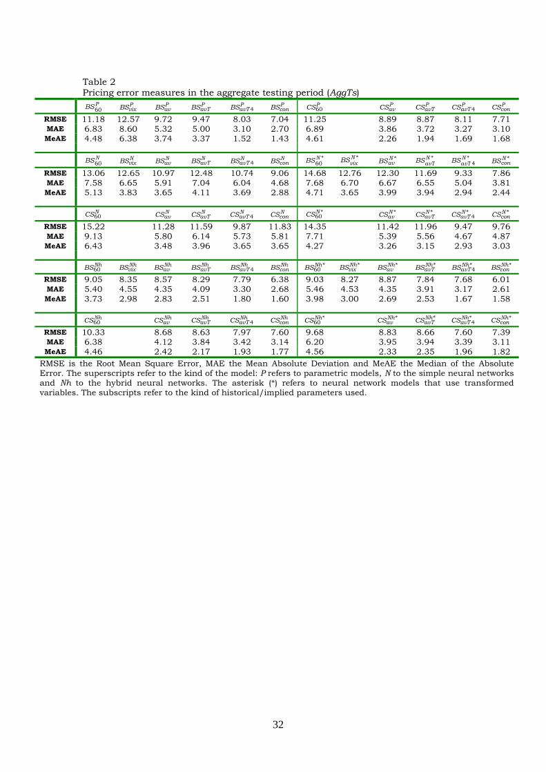
Table 2, exhibits the performance of all parametric and ANN models

considered in this study in terms of RMSE, MAE and MeAE for the AggTs (aggregate)

period. In Table 3 we tabulate statistics for a pairwise comparison of the (statistical

significance of) pricing performance of a selection of models. Since the ten testing periods are disjoint and because we have pricing estimates coming from different

OPMs we can assume (similarly to Hutchison et al, 1994 and Schittenkopf and

Dorffner, 2001) that the pricing errors are independent and standard t-test can be

applied. Similarly to the previous authors we need to report that these tests should

be interpreted with caution. The upper diagonal of Table 3 reports the t-values taken

by a two-tail matched-pair test about the MAE of the alternative models whilst the

lower diagonal exhibits the two-tail matched-pair t-test values about the MSE of the

compared OPMs. Table 4 provides (as a robustness check) the performance of the

models when using the reduced dataset.

[Table 2, 3 and 4, here]

5 The RMSE for CS in the fourth step (con) is 1.82 (caused by a tiny part of the dataset less than 0.1%) due to binding constraints on skewness and kurtosis. For this step, the MeAE is more appropriate, and is effectively zero. The RMSE and the MeAE for BS in the fourth step are effectively zero.

16

By looking at Tables 2 and 4 we can see that the use of implied instead of

historical parameters improves performance, both for parametric and ANN models

(in both datasets). Note that the 60-day historical volatility performed better than

VIX with the parametric BS model, but the VIX volatility measure performed better

with the ANN models. Using time adjusted parameters in the ANNs or using contract

specific parameters {avT4, con} usually improves performance. The combination of

time adjusted parameters and contract specific parameters always provided the best

model within each class of ANNs (standard or hybrid, BS or CS based) in both

datasets.

In comparing the parametric models and again looking at Tables 2 and 4, it is

noteworthy that CS outperforms BS when average implied parameters are used. BS

still works better with contract specific parameters. The overall best among the

parametric models is the contract specific BS model. In other more complex

parametric models that include jumps and stochastic volatility components (i.e.

Bakshi et al., 1997), deriving implied parameters may lead to model overfitting. The

contract specific approach we adopt in this study seems not to lead to model

overfitting, retaining thus good out-of-sample properties. For the ANN models, the

CS based may outperform the BS based in some cases, but when the best

combinations are used (time adjusted parameters and contract specific parameters),

the best model always is BS based in both the standard and hybrid networks.

In comparing the parametric models with the standard ANNs, in the full

dataset the ANNs never outperform the equivalent parametric ones. Apparently, the

standard ANNs cannot perform well in the extreme data regions. In the reduced

dataset (see Table 4), we observe the opposite since the standard ANNs always

outperform the equivalent parametric ones.

In comparing the hybrid with the standard ANNs, in the full dataset the

hybrid are always better. In the reduced dataset this may not always be the case, but

the best combinations (time adjusted parameters and contract specific parameters)

give as the best model always a hybrid one.

In both the full and the reduced dataset, the hybrid always outperform the

equivalent parametric ones. Finally, in both the full and the reduced dataset, the

overall best model is the BS based hybrid with time adjusted and contract specific

volatility.

From Table 3, we can confirm the statistical significance of the best models.

The comparative results we discuss with tests using the full dataset, and they also

hold for the reduced dataset (statistics not reported for brevity). We can see that

17

*NhconBS outperforms all other models. Specifically, *Nh

conBS is producing a RMSE equal

to 6.01 and a MAE equal to 2.61, pricing measures that are smaller that any other

model at the 5% significance level.

The BS based hybrid ANNs even with historical or the VIX volatility measure

are considerably better than the equivalent parametric alternatives at a statistically

significant level. Specifically, *60NhBS is producing 1.23 (1.25) times smaller MSE

(MAE) compared to 60PBS . Also *Nh

vixBS produces 1.52 (1.90) times smaller MSE (MAE)

compared to PvixBS .

Comparing the out-of-sample pricing performance of *NhconBS to *Nh

conCS we

observe that the extra ANN flexibility of the latter due to the two additional input

parameters does not lead to increased accuracy. The *NhconBS is better than the *Nh

conCS

model at 1% significance level.

We can similarly see the statistical significance of the superiority of the BS

based models with contract specific volatility versus the equivalent CS based models

(both parametric and hybrid); and the superiority of the models using the implied

volatility versus the equivalent ones using the historical volatility measures.

5.3. Other statistics

We tabulate in Table 5 the MSE of a selective (but representative) choice of

models, according to the various moneyness and maturity classes for the aggregate

(AggTs) period. We demonstrate results for the two best performing parametric

models which serve as benchmark ( PconBS , P

conCS ,) and the two best performing (in

their respective class) hybrid ANN models ( *NhconBS , *Nh

conCS ). We also demonstrate

results for the reduced dataset ( *NhconBS , *Nh

conCS ). The relevant information for the

parametric models in the reduced dataset can be taken from the information

concerning the full if we ignore the long maturities, and the VDOTM and the VDITM

classes. Very briefly, what can be seen is that PconBS has a smaller RMSE in all data

classes compared to PconCS . The same holds for *Nh

conBS over *NhconCS . If we compare the

BS and CS based hybrid models with the equivalent parametric ones, the hybrid

ANN models rarely underperform the parametric ones, and they do so only in some

classes far away from ATM. This we attribute to the scarcity of such call option

datapoints in the training samples compared to other moneyness and maturity

classes.

[Table 5, here]

18

We should finally comment on the complexity of each neural network

configuration. Since we have a constant number of inputs within each model class,

the larger the number of hidden neurons the more complex the ANN model

architecture, and the more complex the target function to be approximated. Firstly,

we observe that the number of hidden neurons changes significantly between sub-

periods. This contradicts many previous studies that employ the assumption that

the market’s options pricing mechanism is the same for all periods examined and

that a constant ANN structure is sufficient. Secondly, the standard target function is

more complex compared to the hybrid one, hence this hybrid category of networks

can perform better in out-of-sample pricing. Thus, it is not surprising that the best

performing ANN model, *NhconBS , demonstrates the simplest structure with an average

of 3.2 hidden layer neurons, compared to the 8 hidden layer neurons in the case of

the equivalent standard ANN ( *NconBS ). Similarly for the CS-based ANNs, we have 4.9

(for *NhconCS ) and 7.7 (for *N

conCS ) hidden layer neurons respectively. Similar network

complexities (not reported) were observed in the reduced dataset.

6. Delta neutral trading strategies

We now investigate the economic significance of the best performing models in

options trading. In order to save space we discuss the parametric versions of BS and

CS which are usually the benchmark, and the hybrid ANN models which provided

the overall best performance. Other studies usually restrict their analysis only to a

hedging investigation of various alternative OPM models (i.e. Hutchison et al., 1994,

Garcia and Gencay, 2000, Schittenkopf and Dorffner, 2001) and avoid exploiting

trading strategies. It is known from previous studies that the best OPM in terms of

out-of-sample pricing performance does not always prove to be the best solution

when we consider delta hedging, since ANNs are optimized based on a pricing error

criterion. Instead, and following the spirit of Black and Scholes (1972), Galai (1977),

and Whaley (1982), we investigate the economic significance of the OPMs by

implementing trading strategies. “A model that consistently achieves to identify

mispriced options and within a time period produces an amount of trading profits

will always be preferred by a practitioner” (Black and Scholes, 1972). The trading

profitability that we will document, indirectly also hints to potential option market

inefficiencies, although testing market efficiency is beyond the scope of our study.

We implement trading strategies based on single instrument hedging, as for example

in Bakshi et al. (1997). In addition, we consider various levels of transaction costs,

19

and we focus on dynamic strategies that are cost-effective. We later extend the

analysis by implementing a modified approach for trading using hedging ratios

obtained via the (widely neglected) Chen and Johnson (1985) method. To our

knowledge, this is the first effort to validate this modified trading strategy using both

parametric and ANN OPMs.

In the trading strategy we implement, we create portfolios by buying (selling)

options undervalued (overvalued) relative to a model’s prediction and taking a delta

hedging position in the underlying asset. This (single-instrument) delta hedging

follows the no-arbitrage strategy of Black and Scholes (1973), where a portfolio

including a short (long) position in a call is hedged via a long (short) position in the

underlying asset, and the hedged portfolio rebalancing takes place in discrete time

intervals (in an optimal manner, not necessarily daily). At time t, if according to the

model the mth call option contract is overvalued (undervalued) relative to its market

value, ,mrkm tc , we go short (long) in this contract and we go long (short) in ,

km tΔ “index

shares6”, where k denotes the relevant model. Then we invest the residual, ,m tB , in a

riskless bond. Note that ,km tΔ is the partial derivative of the option price with respect

to the underlying asset, , /km t tc S∂ ∂ , depending on the OPM under consideration. ,

ANNm tΔ

can be calculated by differentiating Equation 4 via the chain rule. The expression for

,BSm tΔ is 1( )Te N dδ− and is derived from Equation 2.1. The expression for ,

CSm tΔ includes

,BSm tΔ and is:

, , 3 3 4 4( 3)CS BSm t m t μ μΔ = Δ + Φ + − Φ , (13)

where 33

QS

∂Φ =

∂ and 4

4QS

∂Φ =

∂ are given below:

3 2 23 1 1 1 1

1 (( ) ( ) ( )[3( ) 3 ( ) 1])3!

e d n d T d T dδ σ σ σ− ΤΦ = Τ Ν + − + − , (13.a)

4 3 24 1 1 1 1 1

2 31 1 1 1 1 1

1 (( ) ( ) 4 ( )(( ) 6( ) ( )( ) 4 ( )( )4!

4( ) ( )( ) 3( ) ( ) ( ) ( )).

e T N d n d T d n d T n d T

d n d T d n d d n d

δ σ σ σ σ

σ

− ΤΦ = + − − +

+ − (13.b)

In general we avoid a naive (expensive) trading strategy with daily rebalancing,

since in the presence of transaction costs this would become prohibitively expensive. 6 Similarly to Bakshi et al. (1997) we assume that the spot S&P 500 index is a traded security.

20

Instead, the position is held as long as the call is undervalued (overvalued) without

necessarily daily rebalancing. Then the position is liquidated and the profit or loss is

computed, tabulated separately and a new position is generated according to the

prevailing conditions in the options market. This procedure is carried out for all

contracts included in the dataset. We rebalance our position in the underlying asset

to keep the appropriate hedge ratio. Rebalanced positions in the index, ,m t tV +Δ , and

the bond, ,m t tB +Δ , are according to:

, , ,( )m t t t t m t t m tV S+Δ +Δ +Δ= ± Δ − Δ , and , , ,r t

m t t m t m t tB B e VΔ+Δ +Δ= + , (14)

where the positive sign is considered when we treat undervalued and the negative

sign when we treat overvalued options. Note that in all trading strategies, when we

need to invest money we borrow and pay the riskless rate; similarly we do for as long

as a strategy provides losses. Thus, when we present profits they are always above

the dollar return on the riskless rate.

Computed statistics include the total profit or loss (P&L), the number of

trades (# Trades), the total profit or loss at 0.2% transaction costs, P&L (0.2%), and

0.4% transaction costs, P&L (0.4%). The (proportional) transaction costs are paid for

both positions (in the call option and in the “index shares”)7. We also implement

strategies with enhanced cost-effectiveness by ignoring trades that involve call

options whose absolute percentage mispricing error, | |/k mrk kc c c− , is less than a

mispricing margin d = 15%, found as P&L (d = 15%). In addition, for these strategies,

we also calculate P&L under aggregate transaction costs for the “index shares”. With

such aggregation, transactions in the underlying assets are paid on the net

(aggregate) exposure of ,m t tV +Δ and not on each position individually. Under this

strategy, we expect additional cost savings that may provide profits even at rather

high transaction cost levels. We use the prefix Agg. in front of P&L to indicate this

strategy. The following observations refer to the full dataset, but they also hold for

the reduced one (unreported due to brevity considerations).

The results for the parametric BS and CS models are tabulated in Panel A of

Tables 6 and 7 respectively. We observe that all models before transaction costs

produce significant profits, implying that both BS and CS can successfully identify

mispriced options. Within BS models the magnitude of P&L is larger for PconBS that

7 For example, assume that the index is at 1300 and a call option has a market price equal to 25 index points and a delta value of 0.60. Under 0.4% transaction costs the total commissions paid (for a single trade) will be 3.22 index points. In the AggTs period the S&P 500 was in a range from about 1100 to 1500. This level of transaction costs is low but attainable by professional traders and market makers.

21

employs a more sophisticated implied volatility forecast. Note though that the more

sophisticated volatility forecast that is used with BS, the larger the number of trades.

So, when 0.2% transaction costs are taken into consideration, all models produce

significant losses and the previous profit dominance of PconBS over 60

PBS reverts

because the latter model incurs less transaction costs (since it engages in a smaller

number of trades). Similar results hold for the CS models although 4PavTCS generates

slightly higher profits compared to PconCS . Realizing that our simpler trading strategy

does not discriminate between high or low expected trading profits, we compute P&L

when trades occur only when an expected profit of at least d = 15% is expected. Now

we observe that all models can be profitable even under 0.4% transaction costs.

Overall we may conclude the following. First, without transaction costs, the

CS models produce higher P&L than their counterpart BS models. This is expected

since the delta values generated by CS models are consistently higher than those of

BS models (for example the median delta values of PconBS for AggTs is 0.632 whilst

for PconCS is 0.697), making CS based trading more aggressive. Moreover, CS with {av}

and {avT} volatility measures, outperforms significantly the equivalent BS models

since it generates more than twice the number of trades; this may happen because

unlike the BS models whose implied volatility changes more smoothly, CS models

implied skewness and kurtosis can change more erratically. Secondly, and for the

same reason, CS models under 0.2% or 0.4% transaction costs become inferior to

their BS counterparts. Thirdly, from unreported calculations we have seen that as d increases we generally observe P&L to increase in a diminishing fashion indicating

that there is an optimal d for maximizing trading profits. Finally, trading “in

aggregate” positions leads to significant further savings on transaction costs.

[Tables 6-8, here]

In Table 8 we present results for the trading strategies based on ANNs (only

for the hybrid models with time adjusted parameters). In general we observe similar

results to those of the parametric models. Contrary though to the parametric OPMs,

the ANNs offer significant improvement in the cases of less sophisticated parameter

estimates. For example, *NhavBS produces a P&L equal to 32,908 compared to a P&L

equal to 14,088 in the case of PavBS . The best models provide profits in 77%-82% of

transactions (detailed figures not reported for brevity) using both the full and the

reduced dataset. Finally, in the presence of transaction costs the BS based hybrid

model with contract specific volatility is not only the best performing ANN model, but

also the overall best. A final observation is that the ability to generate profits even

22

under a considerable level of transaction costs (we do not report here, but the best

strategies retained profitability even up to a level of 0.5% of transaction costs)

provides some evidence of inefficiency in these options markets. Our study however

is not intended to be a test of market efficiency.

6.1. Improving trading performance with the Chen and Johnson (1985) modified hedging approach

We now extend the trading strategies by utilizing with all models the improved

hedging scheme suggested by Chen and Johnson (1985). This is a widely neglected

(see Roon et al., 1998 for a rare exception in the use of parametric models) approach

that deals with deriving hedge parameters under the assumption of mispriced

options. According to this hedging scheme and when an option is mispriced, the

delta hedge parameter, ,km tΔ , should be derived in a different way. If a mispriced

option has been identified, then the riskless hedge will not earn r, the riskless rate,

but some other rate, r*. Chen and Johnson obtain the expression for a European call

option that is the same as BS presented in Equations 1, 1.a and 1.b, by replacing r with r*. In order to derive the correct hedge ratio, Equation 1 must be solved

numerically for r* using the observed market price of cmrk (like retrieving the implied

interest rate). We implement this approach with the parametric BS and CS models,

and the ANNs.

Finding the implied interest rate, r*, for the case of BS or CS is a simple

numerical task and we employ the repeated cubic interpolation technique according

to Charalambous (1992). Finding the implied interest rate, r*, for ANNs is a more

involved task, since in the case of hybrid models we need to jointly optimize with

respect to the interest rate input to the neural networks and to the interest rate in

the parametric model that is used to create the hybrid target function; this

introduces many jagged ridge regions in the optimization surface. Thus, in the case

of hybrid ANNs we adopt a more computationally intensive methodology according to

which we again use the cubic interpolation technique with ten different initial

starting points.

After finding r* for all models considered we rerun the trading strategies.

Results for the parametric BS and CS models appear in Panel B of Tables 6 and 7.

The most important observation is that before transaction costs are accounted for, in

all BS models under consideration there is a slight (only) improvement in their

profitability (P&L). Under aggregate 0.4% transaction costs and for d = 15%, the

improvement in 60PBS is about 19%, in P

vixBS is surprisingly about 164% and for the

23

more sophisticated PconBS model only 1.67%. We remind that P

vixBS exhibited both,

the poorest out-of-sample pricing performance and only a modest profitability (under

0.4% transaction costs) among the BS models. Under the adjusted deltas, this seems

to be partly alleviated. Somewhat similar results we observe for the semi-parametric

CS model. For both parametric models, the modified hedging approach under

transaction costs gave the best results when using the average (not contract specific)

parameters. In the case of ANNs (results unreported for brevity) and under no

transaction costs, we also observe a slight tendency for increased performance, but

the results are mixed. With transaction costs the technique was unable to improve

the profitability of ANNs. The above observations refer to the full dataset, but they

also hold for the reduced one (again not reported due to brevity).

A general observation for the use of the modified hedging approach in trading

strategies is that it significantly improves trading performance when it is applied

with OPM models under assumptions consistent with the assumptions under which

this approach was developed. Thus, it performs well with the parametric models

when either historical, or average implied parameters are used. The use of this

approach did not reverse our previous findings about the best performing models

when trading in the presence of transaction costs. Still, it demonstrated that simple

models can be efficient alternatives to the more sophisticated and computationally

intensive hybrid ANN methods.

6.2. Delta hedging

We have also considered hedging as a testing tool. Our results here coincide

with previous literature – model ranking may differ if testing is based on hedging

instead of pricing. Bakshi et al. (1997) compare alternative parametric models and

state that the hedging-based ranking of the models is in sharp contrast with that

obtained based on out-of-sample pricing. They also state that (delta-hedging)

performance is virtually indistinguishable among models. Quite similar results are

reported in papers where non-parametric methods were used, like Garcia and

Gencay (2000), and Gencay and Qi (2001). Schittenkopf and Dorffner (2001) find the

results (marginally) better for the parametric models, but practically

indistinguishable. Hutchison et al. (1994) also report that the learning networks they

use have a better hedging performance compared to BS but they find it difficult to

infer which network type performs best. We attribute this difference of model ranking

to the fact that models are usually optimized with respect to pricing. An exception is

Carverhill and Cheuk (2003) who focus more on hedging performance by optimizing

24

with respect to the hedge parameters. Optimizing the “hedging performance” is

beyond the scope of our paper. Furthermore, hedging performance is not a

substitute for trading performance, since hedging tests fail to account for the

difference between overpriced and underpriced options.

We have calculated the mean hedging error (MHE) and the mean absolute

hedging error (MAHE) of a standard hedging strategy with daily rebalancing. For

brevity we do not report the full results here, but we have found according to MHE

that the best parametric model is the PconCS . Among the ANN models the best

performing one is *NhconCS , with an identical error for the parametric CS model (equal for

both models to 0.26). In addition, the error equals 0.30 for both the PconBS and the

*NhconBS models. In general, from the MHE we cannot tell which OPM is the best since

their difference in this measure is practically indistinguishable. Continuing with the

MAHE we have the same picture, and we find it hard to observe a certain OPM that

dominates in this measure since many models have “almost identical” MAHE values.

It is true that PconBS and P

avTBS 4 are the overall best models (with MAHE equal to

2.57 for both) and perform relatively better than the ANN models (their hybrid ANN

counterparts both having an error equal to 2.63).

In general, we can conclude that the hedging error performance is not in line

with the models’ pricing performance. That is, our best model in pricing accuracy, *Nh

conBS , does not produce the smallest hedging errors. But again, it is truly hard to

differentiate among models. The above discussion pertains to the full dataset, but we

have observed that ranking models using hedging performance is not affected by the

choice of dataset.

7. Conclusions

Our effort has focused in developing European option pricing and trading

tools by combining the use of ANN methodology and information provided by

parametric OPMs (the BS and the CS model). For our empirical tests we have used

European call options on the S&P 500 Index from January 1998 to August 2001. In

our analysis we have included historical parameters, a VIX volatility proxy derived by

weighting implied volatilities (for the case of BS only), and implied parameters (an

overall average, an average per maturity, the 4-point closest in moneyness, and a

contract-specific parameter set). Neural networks are optimized using a modified

Levenberg-Marquardt training algorithm. We include in the analysis simple ANNs

(with input supplemented by historical or implied parameters specific either to BS or

25

the CS model), and hybrid ANNs that in addition use pricing information derived by

any of the two parametric models. In order to check the robustness of the results, in

addition to our full dataset we repeat the analysis using a reduced dataset (following

Hutchison et al., 1994). The economic significance of the models is investigated

through trading strategies with transaction costs. Instead of naive trading strategies

we implement improved (dynamic and cost-effective) ones. Furthermore, we also

refine these strategies with the Chen and Johnson (1985) modified hedging

approach. Our results can be synopsized as follows:

Regarding the in-sample pricing, CS performs better than the BS model (with

the exception of the case of the contract specific implied parameters that practically

eliminate the pricing error).

Regarding out-of-sample pricing, CS outperforms BS with the use of average

implied parameters, but BS is still a better model when the contract specific implied

parameters are used; in general, implied parameters lead to better performance than

the historical ones or the VIX volatility proxy; the simple neural networks cannot

outperform the parametric models in the full range of data, but we verified

allegations to the contrary found in the literature with the use of a reduced data set;

hybrid neural networks that combine both neural network technology and the

parametric models provide the best performance, especially when contract specific

and adjusted parameters are used. The BS based hybrid ANN (with contract specific

parameters) is the overall best performer, and the equivalent CS hybrid often a good

alternative.

In trading and before transaction costs, models using contract specific implied

parameters provide the best performance. But they also lead to the highest number

of trades. In trading when transaction costs are accounted for in a naive manner,

profits practically in all cases disappear. In trading and even with 0.4% transaction

costs, when dynamic cost-efficient strategies are implemented, profits are still

feasible hinting thus to potential market inefficiencies. The parametric BS with

contract specific volatility is the best among the parametric models. The hybrid ANN

based on BS with contract specific volatility is the overall best.

Implementing the widely neglected Chen and Johnson (1985) modified

hedging approach, improves significantly the profitability of trading strategies that

are based on the parametric models with average implied parameters (the models

more consistent with the assumptions behind the modified hedging approach). This

approach did not affect the choice of the overall best model in terms of trading with

transaction costs. But it did demonstrate that reasonable alternatives for trading do

exist without the need to resort to the extra sophistication of ANN technology.

26

References

Andersen, T.G., Benzoni, L., Lund, J., 2002. An empirical investigation of

continuous-time equity return models, Journal of Finance 57 (3) 1239-1276.

Bakshi, G., Cao, C., Chen, Z., 1997. Empirical performance of alternative options

pricing models, Journal of Finance 52 (5) 2003-2049.

Bakshi, G., Cao, C., Chen, Z., 2000. Pricing and hedging long-term options, Journal

of Econometrics 94 (1-2) 277-318.

Bates, D.S., 1991. The Crash of ’87: Was it expected? The evidence from options

markets, Journal of Finance 46 (3) 1009-1044.

Bates, D.S., 1996. Jumps and stochastic volatility: Exchange rate processes implicit

in Deutsche mark options, The Review of Financial Studies 9 (1) 69-107.

Bates, D.S., 2003. Empirical option pricing: A retrospection, Journal of

Econometrics 116 (1-2) 387-404.

Black, F., Scholes, M., 1972. The valuation of option contracts and a test of market

efficiency, The Journal of Finance 27 (2) 399-417.

Black, F., Scholes, M., 1973. The pricing of options and corporate liabilities, Journal of

Political Economy 81 (3) 637-654.

Black, F., Scholes, M., 1975. Fact and fantasy in the use of options, The Financial

Analysts Journal 31, 36-41 and 61-72.

Brown, C., Robinson, D., 2002. Skewness and kurtosis implied by option prices: A

correction, Journal of Financial Research 25 (2) 279-282.

Canica, L., Figlewski, S., 1993. The informational content of implied volatility, The

Review of Financial Studies 6 (3) 659-681.

Carverhill, A., Cheuk, T.H.F., 2003. Alternative neural network approach for option

pricing and hedging, Working paper, School of Business, University of Hong Kong.

Charalambous, C., 1992. A conjugate gradient algorithm for efficient training of

artificial neural networks, IEE Proceedings – G, 139, 301-310.

Chen, N., Johnson, H., 1985. Hedging options, Journal of Financial Economics 14

(2) 317-321.

Cont, R., Fonseca, J., 2002. Dynamics of implied volatility surfaces, Quantitative

Finance 2 (1) 45-60.

Corrado, C.J., Su, T., 1996. Skewness and kurtosis in S&P 500 index returns

implied by option prices, Journal of Financial Research 19 (2) 175-192.

Cybenko, G., 1989. Approximation by superpositions of a sigmoidal function,

Mathematics of Control, Signal and Systems 2, 303-314. Galai, D., 1977. Tests of market efficiency of the Chicago Board Options Exchange,

The Journal of Business 50 (2) 167-197.

27

Garcia, R., Gencay, R., 2000. Pricing and hedging derivative securities with neural

networks and a homogeneity hint, Journal of Econometrics 94 (1-2) 93-115.

Gencay, R., and Qi, M., 2001. Pricing and hedging derivative securities with neural

networks: Bayesian regularization, early stopping and bagging, IEEE Transactions

on Neural Networks 12 (4) 726-734.

Gultekin, N.B., Rogalski, R.J., Tinic S.M., 1982. Option pricing models estimates:

some empirical results, Financial Management 11, 58-69.

Hagan, M., Demuth, H., Beale, M., 1996. Neural Network Design, PWS Publishing

Company.

Hagan, M.T., Menhaj, M., 1994. Training feedforward networks with the Marquardt

algorithm, IEEE Transactions on Neural Networks 5 (6) 989-993.

Hull, C.J., 1999. Options Futures and Other Derivatives, Prentice-Hall (4th edition).

Hutchison, J.M., Lo, A.W., Poggio, T., 1994. A nonparametric approach to pricing

and hedging derivative securities via learning networks, Journal of Finance 49 (3)

851-889.

Lajbcygier P., Boek C., Palaniswami M., Flitman A., 1996. Comparing conventional

and artificial neural network models for the pricing of options on futures, Neurovest

Journal 4 (5) 16-24.

Lajbcygier, P., Flitman, A., Swan, A., Hyndman, R., 1997. The pricing and trading of

options using a hybrid neural network model with historical volatility, Neurovest

Journal 5 (1) 27-41.

Latane, H.A., Rendleman, R.J. Jr., 1976. Standard deviations of stock price ratios

implied in option prices, The Journal of Finance 31 (2) 369-381.

MacBeth, J.D., Merville, L.J., 1980. Tests of the Black-Scholes and Cox call option

valuation models, Journal of Finance 35 (2) 285-301.

Merton, R.C., 1973, Theory of rational option pricing, Bell Journal of Economics and

Management Science 4 (Spring) 141-183.

Roon, De F., Veld C., Wei, J., 1998. A study on the efficiency of the market for Dutch

long-term call options, European Journal of Finance 4 (2) 93-111.

Rubinstein, M., 1985. Nonparametric tests of alternative option pricing models using

all reported trades and quotes on the 30 most active CBOE option classes from

August 23, 1976 through August 31, 1978, The Journal of Finance 40 (2) 455-480.

Schittenkopf C., Dorffner, G., 2001. Risk-neutral density extraction from option

prices: Improved pricing with mixture density networks, IEEE Transactions on

Neural Networks 12 (4) 716-725.

Vahamaa, S., 2003. Skewness and kurtosis adjusted Black-Scholes model: A note on

hedging performance, Finance Letters 1(5).

28

Watson, P., Gupta, K.C., 1996. EM-ANN models for microstript vias and

interconnects in dataset circuits, IEEE Transactions on Microwave Theory and

Techniques 44 (12) 2495-2503.

Whaley, R.E., 1982. Valuation of American Call Options on dividend-paying stocks,

The Journal of Financial Economics 10 (1) 29-58.

Yao, J., Li, Y., Tan, C.L., 2000. Option price forecasting using neural networks, The

International Journal of Management Science 28 (4) 455-466.

29

Fig. 1. A single hidden layer feedforward neural network

H

2

fH(.)

fH(.)

fH(.)

1 f0(.)

1

Input Layer Hidden Layer Output Layer

)1(1ψ

)1(2ψ

)1(Hψ

)1(1y

)1(2y

)1(Hy

ψ y

1x0 ≡

1x

2x

Nx

1b

2b

Hb

11w12w

12w Nw1

N2w

1Hw

HNw

N1w

2Hw

22w

1y )1(0 ≡

1v

2v

Hv

0v

30

Tr1 Vd1 Ts1 Tr2 Vd2 Ts2

… … … … … … … … … … … … Tr10 Vd10 Ts10

Fig. 2. The rolling-over training/validation/testing procedure

Training set Validation set Testing set

Period under examination

31

Table 1 Sample descriptive statistics

VDOTM DOTM OTM JOTM ATM JITM ITM DITM VDITM

S/X <0.85 0.85-0.95

0.90-0.95

0.95-0.99

0.99-1.01

1.01-1.05

1.05-1.10

1.10-1.35 ≥1.35

Short Term Options <60 Days Call 3.61 1.63 5.15 15.70 32.40 56.58 99.55 199.77 470.38

volatility 0.36 0.21 0.19 0.19 0.20 0.22 0.27 0.38 0.99 # obs 399 1,361 4,815 7,483 3,964 6,548 4,970 7,990 2,103

Medium Term Options 60-180 Days Call 4.38 8.29 23.58 46.06 64.51 90.35 131.10 227.41 493.18

volatility 0.22 0.18 0.20 0.21 0.21 0.23 0.25 0.30 0.54 # obs 1,412 1,727 2,578 3,147 1,780 2,901 3,038 8,100 3,999

Long Term Options ≥ 180 Days Call 9.65 42.09 74.03 106.24 126.03 150.99 185.87 267.12 495.82

Volatility 0.18 0.21 0.22 0.23 0.24 0.25 0.26 0.28 0.40 # obs 332 333 575 603 343 660 812 2,695 1,733

Sample characteristics for the period January 5, 1998 to August 24, 2001 concerning the average call option value, the average Black and Scholes contract specific implied volatility and the number of observations in each moneyness/maturity class.

32

Table 2 Pricing error measures in the aggregate testing period (AggTs)

PBS60 P

vixBS PavBS P

avTBS PavTBS 4

PconBS PCS60

PavCS P

avTCS PavTCS 4

PconCS

RMSE 11.18 12.57 9.72 9.47 8.03 7.04 11.25 8.89 8.87 8.11 7.71 MAE 6.83 8.60 5.32 5.00 3.10 2.70 6.89 3.86 3.72 3.27 3.10 MeAE 4.48 6.38 3.74 3.37 1.52 1.43 4.61 2.26 1.94 1.69 1.68

NBS60 N

vixBS NavBS N

avTBS NavTBS 4

NconBS *NBS60

*NvixBS *N

avBS *NavTBS *N

avTBS 4 *N

conBS RMSE 13.06 12.65 10.97 12.48 10.74 9.06 14.68 12.76 12.30 11.69 9.33 7.86 MAE 7.58 6.65 5.91 7.04 6.04 4.68 7.68 6.70 6.67 6.55 5.04 3.81 MeAE 5.13 3.83 3.65 4.11 3.69 2.88 4.71 3.65 3.99 3.94 2.94 2.44

NCS60 N

avCS NavTCS N

avTCS 4 N

conCS *NCS60 *N

avCS *NavTCS *N

avTCS 4 *N

conCS RMSE 15.22 11.28 11.59 9.87 11.83 14.35 11.42 11.96 9.47 9.76 MAE 9.13 5.80 6.14 5.73 5.81 7.71 5.39 5.56 4.67 4.87 MeAE 6.43 3.48 3.96 3.65 3.65 4.27 3.26 3.15 2.93 3.03

NhBS60

NhvixBS Nh

avBS NhavTBS Nh

avTBS 4 Nh

conBS *NhBS60 *Nh

vixBS *NhavBS *Nh

avTBS *NhavTBS 4

*NhconBS

RMSE 9.05 8.35 8.57 8.29 7.79 6.38 9.03 8.27 8.87 7.84 7.68 6.01 MAE 5.40 4.55 4.35 4.09 3.30 2.68 5.46 4.53 4.35 3.91 3.17 2.61 MeAE 3.73 2.98 2.83 2.51 1.80 1.60 3.98 3.00 2.69 2.53 1.67 1.58

NhCS60

NhavCS Nh

avTCS NhavTCS 4

NhconCS *NhCS60

*NhavCS *Nh

avTCS *NhavTCS 4

*NhconCS

RMSE 10.33 8.68 8.63 7.97 7.60 9.68 8.83 8.66 7.60 7.39 MAE 6.38 4.12 3.84 3.42 3.14 6.20 3.95 3.94 3.39 3.11 MeAE 4.46 2.42 2.17 1.93 1.77 4.56 2.33 2.35 1.96 1.82

RMSE is the Root Mean Square Error, MAE the Mean Absolute Deviation and MeAE the Median of the Absolute Error. The superscripts refer to the kind of the model: P refers to parametric models, N to the simple neural networks and Nh to the hybrid neural networks. The asterisk (*) refers to neural network models that use transformed variables. The subscripts refer to the kind of historical/implied parameters used.

33

Table 3 Matched-pair student t-tests for square and absolute differences

PBS60 P

vixBS PconBS PCS60

PconCS *NBS60

*NCS60 *NhBS60

*NhvixBS *Nh

conBS *NhCS60 *Nh

conCS PBS60

-27.74 75.12 -0.94 65.72 -11.07 -11.72 23.90 40.83 81.22 10.80 66.92 PvixBS 7.17 104.84 26.74 94.84 11.84 11.71 53.72 70.71 112.32 40.52 96.53 PconBS -16.13 -25.08 -75.91 -8.43 -70.51 -72.82 -56.94 -38.56 2.12 -70.87 -8.76 PCS60

0.34 -6.72 16.31 66.53 -10.28 -10.91 24.85 41.74 82.02 11.78 67.74 PconCS -13.38 -21.60 2.14 -13.58 -63.58 -65.63 -46.76 -28.85 11.11 -60.38 -0.10

*NBS60 7.24 4.64 13.37 7.09 12.48 -0.34 30.64 43.94 74.23 20.23 64.28

*NCS60 7.77 4.67 15.19 7.59 14.09 -0.62 31.84 45.50 76.80 21.15 66.39

*NhBS60 -9.55 -18.30 7.57 -9.81 4.95 -10.83 -12.15 18.64 63.30 -14.28 47.82

*NhvixBS -12.54 -21.61 4.48 -12.75 2.02 -11.91 -13.46 -3.25 43.70 -32.87 29.50

*NhconBS -21.16 -32.03 -3.45 -21.26 -5.62 -14.65 -16.83 -12.27 -8.78 -78.03 -11.58

*NhCS60 -6.86 -15.36 10.42 -7.15 7.65 -9.84 -10.96 2.97 6.24 15.52 61.73

*NhconCS -14.98 -23.78 1.15 -15.16 -1.04 -12.95 -14.69 -6.34 -3.26 4.73 -9.18

Reported matched-pair t-tests concerning the absolute differences are in the upper diagonal, whilst the matched-pair t-tests concerning the square differences in the lower diagonal. Both tests compare the MAE and MSE between models in the vertical heading versus models in the horizontal heading. In general, a positive t-value larger than 1.645 (2.325) means that the model in the vertical heading has a larger MAE or MSE than the model in the horizontal heading at 5% (1%) significance level.

34

Table 4 Pricing error measures in the aggregate testing period (AggTs) for the reduced dataset

PBS60 P

vixBS PavBS P

avTBS PavTBS 4

PconBS PCS60

PavCS P

avTCS PavTCS 4

PconCS

RMSE 9.83 11.82 8.41 8.25 7.08 7.06 9.74 7.56 7.55 7.55 7.52 MAE 6.35 8.43 4.82 4.54 2.65 2.65 6.32 3.38 3.12 2.99 3.04 MeAE 4.50 6.57 3.63 3.27 1.48 1.46 4.59 2.17 1.83 1.69 1.71

NBS60 N

vixBS NavBS N

avTBS NavTBS 4

NconBS *NBS60

*NvixBS *N

avBS *NavTBS *N

avTBS 4 *N

conBS RMSE 8.05 6.56 7.34 6.94 6.64 6.69 7.14 6.60 6.82 6.91 6.25 6.12 MAE 5.07 3.34 4.02 3.72 3.42 3.37 4.11 3.43 3.46 3.59 3.01 3.00 MeAE 3.80 2.32 2.99 2.56 2.33 2.24 3.09 2.41 2.44 2.56 1.99 2.02

NCS60 N

avCS NavTCS N

avTCS 4 N

conCS *NCS60 *N

avCS *NavTCS *N

avTCS 4 *N

conCS RMSE 9.05 7.18 6.93 6.94 6.88 8.35 6.97 6.59 6.50 6.77 MAE 5.74 3.95 3.61 3.73 3.62 4.94 3.68 3.26 3.23 3.45 MeAE 4.25 2.74 2.41 2.60 2.55 3.43 2.62 2.22 2.25 2.36

NhBS60 Nh

vixBS NhavBS Nh

avTBS NhavTBS 4

NhconBS *NhBS60

*NhvixBS *Nh

avBS *NhavTBS *Nh

avTBS 4 *Nh

conBS

RMSE 8.45 6.70 7.29 7.01 6.58 6.78 7.35 6.40 7.05 6.83 5.94 5.64 MAE 5.11 3.58 3.62 3.38 2.62 2.69 4.27 3.21 3.32 3.30 2.45 2.44 MeAE 3.44 2.59 2.55 2.35 1.55 1.65 3.13 2.26 2.30 2.33 1.51 1.54

NhCS60

NhavCS Nh

avTCS NhavTCS 4

NhconCS *NhCS60

*NhavCS *Nh

avTCS *NhavTCS 4

*NhconCS

RMSE 7.80 7.29 6.83 7.31 7.35 7.69 6.90 6.80 6.51 6.46 MAE 4.65 3.20 3.08 3.03 3.03 4.58 3.13 2.92 2.83 2.87 MeAE 3.41 2.13 2.02 1.82 1.80 3.23 2.03 1.80 1.79 1.81

RMSE is the Root Mean Square Error, MAE the Mean Absolute Error and MeAE the Median of the Absolute Error. The superscripts refer to the kind of the model: P refers to parametric models, N to the simple neural networks and Nh to the hybrid neural networks. The asterisk (*) refers to neural network models that use the transformed variables. The subscripts refer to the kind of historical/implied parameters used.

35

Table 5 Root Mean Square Errors for selected models (clustered by moneyness and maturity)

Short Medium Long Short Medium Long Results for the full dataset P

conBS PconCS

VDOTM 3.60 4.91 0.56 8.34 10.61 0.66 DOTM 2.27 4.50 2.82 3.02 5.24 4.47 OTM 5.78 8.37 3.97 6.29 9.68 5.08 JOTM 7.81 6.68 6.15 8.13 7.64 7.65 ATM 6.67 9.46 5.86 7.30 10.14 7.29 JITM 6.71 9.41 4.34 7.29 9.21 5.97 ITM 7.70 7.13 4.43 8.24 7.59 5.18

DITM 7.07 7.93 7.27 7.20 8.50 7.50 VDITM 8.26 9.46 8.74 8.29 10.05 9.05

*NhconBS *Nh

conCS

VDOTM 3.60 4.97 1.15 6.13 10.22 6.04 DOTM 2.46 4.83 2.32 2.96 5.28 5.03 OTM 5.50 7.75 3.98 6.19 9.41 5.36 JOTM 5.89 5.36 5.78 7.83 7.30 7.66 ATM 4.73 8.18 5.38 6.94 9.86 7.13 JITM 5.59 7.39 4.10 6.89 8.68 6.64 ITM 6.24 6.05 3.95 7.58 7.16 5.69

DITM 5.80 7.15 6.74 6.64 8.04 7.17 VDITM 8.03 9.29 8.46 8.96 10.33 9.26

Results for the reduced dataset *Nh

conBS *NhconCS

VDOTM n.a. n.a. n.a. n.a. n.a. n.a. DOTM 2.36 4.07 n.a. 2.54 5.22 n.a. OTM 5.08 7.25 n.a. 5.69 8.74 n.a. JOTM 5.82 5.59 n.a. 6.76 7.09 n.a. ATM 4.65 8.37 n.a. 5.68 9.53 n.a. JITM 5.50 7.68 n.a. 6.20 8.16 n.a. ITM 5.98 5.84 n.a. 6.73 6.75 n.a.

DITM 5.45 6.59 n.a. 5.95 7.67 n.a. VDITM n.a. n.a. n.a. n.a. n.a. n.a.

36

Table 6 Trading strategies for the Black and Scholes models

PBS60 P

vixBS PavBS P

avTBS PavTBS 4

PconBS

Panel A: Black and Scholes trading strategy with standard delta values P&L 7,447 13,518 14,088 13,069 32,040 35,026

# Trades 3,361 3,878 4,858 5,477 13,539 15,644 P&L 0.2% (d=0%) -6,829 -6,847 -5,348 -7,512 -17,911 -23,307

Agg P&L 0.2% (d=0%) -1,861 -266 737 -1,394 -5,638 -8,437 P&L 0.2% (d=15%) 3,320 4,134 7,527 6,841 7,907 7,369

Agg P&L 0.2% (d=15%) 5,003 5,019 8,344 7,657 8,384 7,873 P&L 0.4% (d=0%) -21,105 -27,211 -24,785 -28,093 -67,863 -81,640

Agg P&L 0.4% (d=0%) -11,170 -14,049 -12,614 -15,858 -43,316 -51,899 P&L 0.4% (d=15%) -1,468 -508 3,241 2,269 4,691 4,212

Agg P&L 0.4% (d=15%) 1,897 1,262 4,875 3,901 5,645 5,221 Panel B: Black and Scholes trading strategy with modified delta values

P&L 7,916 14,367 14,232 13,441 32,281 35,229 # Trades -6,169 -5,599 -4,958 -6,946 -17,788 -23,080

P&L 0.2% (d=0%) -1,392 1,342 1,225 -778 -5,534 -8,259 Agg P&L 0.2% (d=0%) 4,044 5,534 8,182 7,546 8,306 7,713

P&L 0.2% (d=15%) 5,515 6,558 9,115 8,524 8,815 8,198 Agg P&L 0.2% (d=15%) -20,254 -25,564 -24,148 -27,334 -67,858 -81,390

P&L 0.4% (d=0%) -10,700 -11,682 -11,782 -14,998 -43,348 -51,748 Agg P&L 0.4% (d=0%) -685 1,284 4,143 3,180 4,883 4,339

P&L 0.4% (d=15%) 2,257 3,333 6,007 5,137 5,900 5,308 P&L is the total profit and loss without transaction costs; # Trades is the number of trades. P&L (d=0 and 15%) represents the P&L at 0.2% or 0.4% transaction costs when we ignore trades whose absolute percentage of mispricing error between model estimates and market values is at least 0% and 15% respectively. Agg. refers to aggregating the position on the underlying asset to reduce transaction costs. Panel A tabulates results with standard delta values whilst Panel B tabulates results with Chen and Johnson modified delta values.

37

Table 7 Trading strategies for the Corrado and Su models

PCS60 P

avCS PavTCS P

avTCS 4 P

conCS

Panel A: Corrado and Su trading strategy with standard delta values P&L 7,603 28,816 32,803 37,072 36,777

# Trades 3,430 11,178 13,306 14,911 15,219 P&L 0.2% (d=0%) -7,658 -15,867 -19,045 -22,750 -24,414

Agg P&L 0.2% (d=0%) -2,532 -4,495 -5,641 -6,685 -6,909 P&L 0.2% (d=15%) 2,868 7,960 6,791 6,606 6,422

Agg P&L 0.2% (d=15%) 4,533 8,739 7,483 7,418 7,311 P&L 0.4% (d=0%) -22,919 -60,550 -70,894 -82,572 -85,604

Agg P&L 0.4% (d=0%) -12,667 -37,805 -44,085 -50,441 -50,595 P&L 0.4% (d=15%) -1,949 2,797 1,935 1,371 1,124

Agg P&L 0.4% (d=15%) 1,383 4,355 3,319 2,993 2,901 Panel B: Corrado and Su trading strategy with modified delta values

P&L 7,837 29,208 33,219 37,044 37,097 # Trades 3,430 11,178 13,306 14,911 15,219

P&L 0.2% (d=0%) -7,209 -15,317 -18,610 -22,828 -24,203 Agg P&L 0.2% (d=0%) -2,332 -3,843 -5,186 -6,708 -6,615

P&L 0.2% (d=15%) 3,512 8,685 7,322 6,740 6,778 Agg P&L 0.2% (d=15%) 4,943 9,539 8,024 7,594 7,720

P&L 0.4% (d=0%) -22,255 -59,841 -70,439 -82,700 -85,503 Agg P&L 0.4% (d=0%) -12,501 -36,893 -43,590 -50,460 -50,328

P&L 0.4% (d=15%) -1,218 3,521 2,303 1,172 1,074 Agg P&L 0.4% (d=15%) 1,646 5,229 3,707 2,881 2,958

P&L is the total profit and loss without transaction costs; # Trades is the number of trades. P&L (d=0 and 15%) represents the P&L at 0.2% or 0.4% transaction costs when we ignore trades whose absolute percentage of mispricing error between model estimates and market values is at least 0% and 15% respectively. Agg. refers to aggregating the position on the underlying asset to reduce transaction costs. Panel A tabulates results with standard delta values whilst Panel B tabulates results with Chen and Johnson modified delta values.

38

Table 8 Trading strategies for the hybrid ANN models

*NhBS60 *Nh

vixBS *NhavBS *Nh

avTBS *NhavTBS 4

*NhconBS

Panel A: Black and Scholes based hybrid ANNs P&L 27,024 29,529 32,908 33,514 35,774 37,281

# Trades 5,675 8,246 8,907 9,457 11,995 12,650 P&L 0.2% (d=0%) 1,694 -4,193 -2,435 -4,134 -11,484 -12,939

Agg P&L 0.2% (d=0%) 10,552 6,053 7,871 7,086 837 1,066 P&L 0.2% (d=15%) 6,593 5,147 8,162 8,579 7,910 8,427

Agg P&L 0.2% (d=15%) 8,247 6,977 9,890 9,957 8,689 9,237 P&L 0.4% (d=0%) -23,637 -37,914 -37,778 -41,782 -58,741 -63,158

Agg P&L 0.4% (d=0%) -5,920 -17,424 -17,166 -19,343 -34,100 -35,148 P&L 0.4% (d=15%) 1,804 -277 2,232 3,156 4,364 4,812

Agg P&L 0.4% (d=15%) 5,112 3,382 5,687 5,911 5,922 6,432

*NhCS60 *Nh

avCS *NhavTCS *Nh

avTCS 4 *Nh

conCS

Panel B: Corrado and Su based hybrid ANNs P&L 26,691 32,915 31,943 34,907 37,975

# Trades 5,140 10,043 10,377 12,537 12,947 P&L 0.2% (d=0%) 3,590 -8,721 -12,019 -17,527 -16,084

Agg P&L 0.2% (d=0%) 11,032 3,734 898 -1,586 735 P&L 0.2% (d=15%) 7,337 6,653 5,601 6,052 7,826

Agg P&L 0.2% (d=15%) 8,861 8,231 7,114 7,439 8,960 P&L 0.4% (d=0%) -19,511 -50,356 -55,980 -69,962 -70,143

Agg P&L 0.4% (d=0%) -4,626 -25,446 -30,146 -38,078 -36,505 P&L 0.4% (d=15%) 2,433 724 457 612 2,605

Agg P&L 0.4% (d=15%) 5,481 3,879 3,484 3,387 4,873 P&L is the total profit and loss without transaction costs; # Trades is the number of trades. P&L (d=0 and 15%) represents the P&L at 0.2% or 0.4% transaction costs when we ignore trades whose absolute percentage of mispricing error between model estimates and market values is at least 0% and 15% respectively. Agg. refers to aggregating the position on the underlying asset to reduce transaction costs. Panel A tabulates results for the hybrid BS based ANN model whilst Panel B tabulates results for the hybrid CS based ANN models.