price setting and competition with search frictions
TRANSCRIPT

Instructions for use
Title Price setting and competition with search frictions
Author(s) Kudoh, Noritaka
Citation Discussion Paper, Series A, 203, 1-29
Issue Date 2009-02
Doc URL http://hdl.handle.net/2115/35514
Type bulletin (article)
File Information DPA203.pdf
Hokkaido University Collection of Scholarly and Academic Papers : HUSCAP

Discussion Paper, Series A, No. 2009-203
Price Setting and Competition
with Search Frictions
Noritaka Kudoh
February, 2009
Graduate School of Economics & Business Administration Hokkaido University
Kita 9 Nishi 7, Kita-Ku, Sapporo 060-0809, JAPAN

Price Setting and Competition with Search Frictions∗
Noritaka Kudoh†
Hokkaido University
Abstract
This paper investigates price determination in a decentralized economy in which buyers’
valuations are stochastic and unobservable. In such a market, each buyer’s reservation utility
depends both on the prevailing price and on the price he actually encounters. The buyer’s
willingness to trade is shown to be decreasing in the price, and this creates the trade-off for
the sellers’ price setting. Even though the sellers have incentives to manipulate the buyer’s
willingness to trade, the economy is not fully competitive; it does not converge to the Walrasian
outcome as search frictions disappear. The model is used to study various market structures
to explore the nature of market power in search equilibrium. It is shown that price dispersion
arises as a result of search frictions and oligopolistic price setting.
JEL classification: C78, D40
Keywords: random search, price setting, competition, oligopoly.
∗I wish to thank Takeshi Yamazaki, Masaru Sasaki, Hiroyuki Adachi, Ryoichi Imai, Shingo Ishiguro, Hideo
Konishi, and the participants of seminars at Hokkaido University, Kansai University, Osaka University (ISER) and
Otaru University of Commerce, and the decentralization conferences at Hosei University and Kinki University for
helpful comments.†Department of Economics, Kita 9 Nishi 7, Kita-ku, Sapporo 060-0809, JAPAN; Email: [email protected]
1

1 Introduction
In textbook microeconomics, buyers behave as price takers. They submit their entire demand
schedules to the Walrasian auctioneer, who aggregates them to produce a single downward-sloping
demand schedule. If firms have some market power, then the demand schedule defines the trade-
off they face between price and quantity. In other words, sellers can (potentially) manipulate the
buyers’ willingness to trade through their prices. In many of the search-matching models, on the
other hand, the terms of trade are determined by bilateral bargaining (Rubinstein and Wolinsky,
1985; Mortensen and Wright, 2002) or by price posting (Acemoglu and Shimer, 1999; Curtis and
Wright, 2004), and the demand manipulation has not been considered.
This paper investigates the sellers’ price setting in search equilibrium in which there is room
for manipulating the buyers’ willingness to trade through their prices. In a random search model,
it is not trivial to obtain a trade-off that is similar to the textbook demand curve.1 As the
analysis in Wolinsky (1986) suggests, the buyers’ willingness to trade is independent of the prices
of commodities if the cost of search is a sampling cost rather than discounting of future utility.2
This paper develops a simple random search model in which discounting captures the degree of
search frictions, and finds an exploitable trade-off between price and the acceptability of trade.
The structure of the model is related to other random search models such as Burdett and
Wright (1998) and in particular Mortensen and Wright (2002). In terms of price setting, this
paper is closely related to Albrecht and Jovanovic (1986) and in particular Masters (1999). The
key features of this paper are: (i) it studies a random two-sided search model of the product market;
(ii) the buyers’ willingness to trade are stochastic and unobservable; (iii) each seller maximizes her
value taking the buyer’s reservation strategy as a constraint ; and (iv) the basic model is extended
to study other market structures such as monopoly and oligopoly.
Throughout this paper, search is two-sided and random. Although the recent development of1There is a growing literature on directed search, where sellers post prices. The tradeoff in that literature is
between price and the queue length. See Acemoglu and Shimer (1999) and Rogerson, Shimer, and Wright (2005) for
expositions.2This point is discussed in Section 4.2 in detail.
2

directed search models is important and to some extent relevant to this paper, I focus on random
search. Part of the reason for this is that the trade-off in the directed search model is between
price and the queue length of buyers. In fact, the key issue in the directed search literature is to
endogenize the matching frictions. The purpose of this paper is to explore how the sellers use the
prices to manipulate the buyers’ willingness to trade in the presence of search frictions.
In many models of decentralized trading, bilateral bargaining is used as the pricing institution.
In particular, either the Nash solution or strategic bargaining (Rubinstein and Wolinsky, 1985)
with observable match surplus is assumed in the literature. With observable valuations, the sellers
would set their prices so that each buyer is just indifferent between accepting and rejecting a
trade. This paper assumes that the buyers’ valuations (or the maximum willingness to pay) are
unobservable. With this realistic assumption, it is shown that each buyer’s search strategy depends
on the prices. In particular, a buyer’s reservation utility depends on the prevailing price of the
commodity and the price he actually faces. The reservation utility is shown to be decreasing in
the price he faces.
This suggests that each seller believes that she can increase the probability that her customer,
who will arrive at the seller’s store at random, will purchase her commodity by cutting her price.
That is, the seller faces an exploitable trade-off between price and acceptability. Technically,
each seller maximizes her value of search, taking the buyer’s reservation strategy as a constraint
(Albrecht and Jovanovic, 1986; Masters, 1999). It is shown that there is a unique search equilibrium
under this pricing scheme.
An important issue in the theory of decentralized trading is to explore the strategic foundation
of general equilibrium (Rubinstein and Wolinsky, 1985; Gale, 1987; Wilson, 1987; Wolinsky, 1988;
De Fraja and Sákovics, 2001; Mortensen and Wright, 2002).3 The present study also intends to
contribute to this important literature. Following the literature, I study the properties of the
basic model in the limit as search frictions disappear. Because of the constant measure of traders
in the steady state (Gale, 1987), the decentralized economy does not converge to the Walrasian
outcome, and the limit price depends on the relative measure of traders (Rubinstein and Wolinsky,3For reviews, see Osborne and Rubinstein (1990) and Gale (2000).
3

1985). It is important to emphasize that the price posting game is not responsible for the non-
Walrasian outcome; the model with observable valuations and bilateral bargaining also leads to
the non-Walrasian outcome.4
As applications of the basic model, this paper considers various forms of market structure. In
the basic model, each seller ignores how her price will influence the buyers’ willingness to trade
through its impact on their values of search (or, the values of their options to wait). The failure
to take into account the equilibrium relationship between price and the willingness to trade has a
profound implication for the competitiveness of the economy. To see this, a monopoly version of
the model is developed, in which all sellers form a single coalition called firm and the firm chooses
the price. From a buyer’s point of view, there are many sellers, but there are no competing sellers.
It is shown that the firm sets a higher price. However, this is not the monopoly price in the
sense of Diamond (1971); the buyers’ values of search are positive because their valuations of the
commodity are unobservable.
The Bertrand Paradox and the Diamond Paradox offer insightful angles to understanding the
nature of competition. The former states that two firms are enough to generate the perfectly
competitive outcome in an oligopoly model with price competition. The latter states that even
with a large number of firms, the monopoly price will result as long as each buyer faces a small
search cost. If there are two firms in a decentralized economy with search frictions, how competitive
will the prices be? I characterize a duopoly version of the model and show that the prices are
strategic substitutes, suggesting that there is no undercutting. In addition, price dispersion arises
as a result of search frictions and oligopolistic price setting, which is new to the literature on price
dispersion. Interestingly, the equilibrium is of the Cournot-type even though the firms compete by
setting prices.
The organization of this paper is as follows. Section 2 presents the basic model and the equi-
librium is studied in Section 3. Some of the results are related to the existing literature in Section
4. Section 5 extends the basic model to study the cases with monopoly and oligopoly. Section 64 In a closely related environment, Mortensen and Wright (2002) showed that their economy generates the Wal-
rasian outcome if potential entrants possess the options to stay out of the market.
4

concludes. All proofs of the main results are presented in the Appendix.
2 The Model
2.1 Environment
Time is continuous, and the time horizon is infinite. There is a continuum of buyers and sellers,
and each individual is atomless. Let r denote the common discount rate. Search is undirected. In
addition, there is no recall. After a trade, the buyer and seller leave the market, and their clones
will replace them (Rubinstein and Wolinsky, 1985; De Fraja and Sákovics, 2001). This assumption
maintains the stationarity of this economy. Thus, although the number of traders at each instant
is finite, it accumulates over time without bound, leading to a non-Walrasian result (Gale, 1987).5
This paper follows Mortensen and Wright (2002) to adopt a general meeting technology. Let
B and S denote the measure of buyers and sellers, respectively. The aggregate pairs made at each
instant are determined by a constant-returns-to-scale function m(B,S), which is increasing in both
arguments. For a buyer, the arrival rate of a trade opportunity is given by m/B ≡ αb, and for a
seller it is m/S ≡ αs. It is easy to verify that αb is decreasing in the buyer—seller ratio B/S ≡ qand αs is increasing. With constant returns, it is easy to verity that αs = q ·αb. It is also assumedthat limq→0 αs = limq→∞ αb = 0 and limq→∞ αs = limq→0 αb =∞.
Each seller produces a common consumption good. It is assumed that the cost of producing
a unit of the commodity is c > 0 and is common to all sellers. All goods are perishable and
indivisible. I assume that production is instantaneous. A buyer’s willingness to trade is stochastic.
Upon meeting, a buyer finds the maximum willingness to pay for a commodity denoted by v. It is
assumed that v is a random draw from distribution F (v), with support [0, v]. It is assumed that
v > c, 0 < F 0 (v) < ∞, and F 00(v) < ∞. A critical assumption is that each realization of v is
unobservable. However, sellers know the distribution F as well as the structure of the economy.5Mortensen and Wright (2002) followed Gale (1987) in assuming stochastic entry of traders and showed that their
economy leads to the Walrasian outcome. De Fraja and Sákovics (2001) obtained the Walrasian outcome even with
the clone assumption by introducing local (or instantaneous) market competition.
5

A possible interpretation of this specification is that consumers’ “mood” changes over time.
The key, however, is that from a seller’s viewpoint, the willingness to pay differs from one buyer to
another. A related assumption is adopted by Wolinsky (1988) and Wang (1995). Alternatively, one
could assume product differentiation (Wolinsky, 1986; Arbatskaya and Konishi, 2005). With this
interpretation, v measures how much a buyer likes a certain commodity, and the market structure
should be interpreted as monopolistic competition. The two specifications are identical as long as
each seller is treated symmetrically.6
The price of a commodity is denoted by p. It should be considered as a utility transfer rather
than a monetary exchange.7 Thus, the instantaneous payoff to a buyer who accepts a trade at
price p is v−p. To simplify the analysis, I focus on a symmetric steady state equilibrium, in whichall sellers follow the same strategy, so there is no price dispersion.
2.2 Buyers
Consider the choice of a typical buyer. Let Vb(p) denote the value of search when the prevailing
price is p.8 Then, the Bellman equation for the buyer is
rVb(p) = αb
Z Z v
0max v − pi − Vb(p), 0 dF (v)dG(pi), (1)
where G(·) is the cumulative distribution function of the price, which is degenerate in equilibrium.Note that v and pi are independent, since a seller, who cannot observe v, cannot condition her
price on v. The reservation strategy requires that the buyer accepts a trade as soon as v ≥ R
holds, where the reservation utility R is given by
R = pi + Vb(p) (2)
for each pi. Thus, the reservation utility is influenced by the prevailing price p and the price posted
by the seller in front of the buyer, pi. In equilibrium, pi = p. It is important to note that, for6The reader who is familiar with Wolinsky (1986) will find it more appropriate to call each seller a monopolistically
competitive firm. Since this paper redefines the term firm later, I shall call individual traders either buyers or sellers.7See Curtis and Wright (2004) for a monetary exchange model with price setting.8 I follow Masters (1999) for this exposition. To be more precise, the value function depends on the entire price
distribution G(p).
6

a given value of search, the reservation utility R increases with pi. This implies that a seller has
an incentive to reduce her price to induce buyers to purchase the commodity from her. This is
somewhat similar to textbook microeconomics, where a seller with some market power faces a
trade-off between price and quantity sold, and the trade-off comes from the consumers’ demand
schedule. Although limited, each seller in this economy has some market power to the extent that
buyers cannot walk away from a seller so easily, because of search frictions.
2.3 Sellers
Each seller is assumed to post a price when searching for a buyer. It is also assumed that sellers
commit to their prices, and price commitment is costless.9 The value to a seller of posting pi when
the prevailing price posted by all other sellers is p, is given by
rVs(pi, p) = αs[1− F (R)][pi − c− Vs(pi, p)], (3)
where 1−F (R) is the probability that a buyer is willing to trade at the posted price pi. If a tradeoccurs, then the seller receives pi, paying the production cost c, and exits the market after the trade.
The key feature of the model is that the arrival rate of a successful trade may be manipulated by
each seller. To see this, the acceptability is written as 1 − F (R) = 1 − F (pi + Vb(p)). Substitutethis into (3) to obtain
rVs(pi, p) = αs[1− F (pi + Vb(p))][pi − c− Vs(pi, p)]. (4)
The seller faces a trade-off in an intuitive manner. If the price is high, her instantaneous utility is
high given that the commodity is sold. On the other hand, a higher price reduces the chance that
the commodity is sold. Facing this trade-off, the seller chooses p to maximize her value of search,
taking all other sellers’ price strategies as given. This is where competition (potentially) comes in.
It is important to emphasize that although a seller can manipulate the acceptability of her
commodity by posting a lower price, search is undirected. This contrasts with the recent directed9Bester (1994) considered a model in which price commitment is costly, and showed that equilibrium with haggling
is possible.
7

search models, in which buyers can quote all prices at no cost and choose (and compete for) a seller
(Acemoglu and Shimer, 1999). In this economy, buyers cannot either choose which sellers to visit
or negotiate the terms of trade; they can only choose whether to accept a trade at the posted price
or to walk away. In this sense, this economy is closer to the one considered by Diamond (1971).
However, here, a seller cannot observe the buyer’s willingness to trade, which effectively prevents
the well-known Diamond Paradox from occurring.
Each seller’s problem is: maxpi Vs(pi, p) subject to R = pi+Vb(p), taking p and therefore Vb as
given. From the seller’s perspective, cutting pi directly improves the buyer’s willingness to trade.
However, the seller fails to take into account how her choice will affect the equilibrium price and
hence the buyer’s value of search.
Proposition 1 Each seller posts
pi = c+[1− F (R)] + (αs/r)[1− F (R)]2
F 0 (R)≡ P (R) , (5)
where P (R) is decreasing if
−1 < F 00(R)F 0(R)2
[1− F (R)] < 2. (6)
Proof. In the Appendix.
The first inequality of condition (6) holds if and only if the survival function 1− F is strictly
log-concave.10 If the density function F 0 is log-concave, then the distribution function F and the
survival function 1−F are log-concave. See Burdett and Wright (1998) and Bagnoli and Bergstrom(2005) for details. Proposition 1 states that the price posting curve is downward sloping if the
density function F 0 is log-concave. The second inequality in (6) is derived from the second-order
condition for the maximization problem. In what follows, I will focus on the economy where (6) is
satisfied.
In what follows, P (R) is referred to as the price posting function. With log-concavity, the
price posting function is decreasing, as shown in Figure 1. Note that a seller perceives r/αs as
the measure of market frictions. It is interesting to observe that as search frictions increase, the10 In general, a function f is log-concave if and only if ff 00 − (f 0)2 ≤ 0.
8

price posting function shifts downward. This suggests that ceteris paribus, greater search frictions
induce each seller to post a lower price.
3 Equilibrium
3.1 Characterization
In any symmetric steady-state equilibrium, all sellers set the same price: pi = p. Thus, distribution
G(·) is degenerate. Use the reservation strategy to rewrite the buyer’s value (1) as
rVb(p) = αb
Z v
R(v −R)dF (v) = αb
Z v
R[1− F (v)]dv. (7)
Substitute (7) into (2) to obtain the equilibrium relationship between p and R as follows:
p = R− αbr
Z v
R[1− F (v)]dv ≡ H(R). (8)
Since H 0(R) = 1 + (αb/r)[1 − F (R)] and H 00(R) = −(αb/r)F 0(R) hold, it is easy to establish thefollowing.
Lemma 2 (a) H 0(R) > 1; (b) H 00(R) < 0; (c) H(0) < 0 and H(v) = v; and (d) H 0(0) = 1+αb/r
and H 0(v) = 1.
Figure 1 depicts the shape of function H(R). This summarizes the equilibrium relationship be-
tween the price and the reservation utility. The steady-state equilibrium is completely characterized
by a pair (p,R) that satisfies (5) and (8), as depicted in the Figure.
Proposition 3 There exists a unique symmetric steady-state equilibrium.
Proof. In the Appendix.
The following reports some results on comparative statics.
Proposition 4 (a) The equilibrium willingness to trade increases with search frictions. (b) The
equilibrium price increases with frictions if and only if
αbαs
[r + αs[1− F (R)]] [1 + C(R)] + αs[1− F (R)]r + αb[1− F (R)] >
[1− F (R)]2F 0 (R)
R vR[1− F (v)]dv
, (9)
9
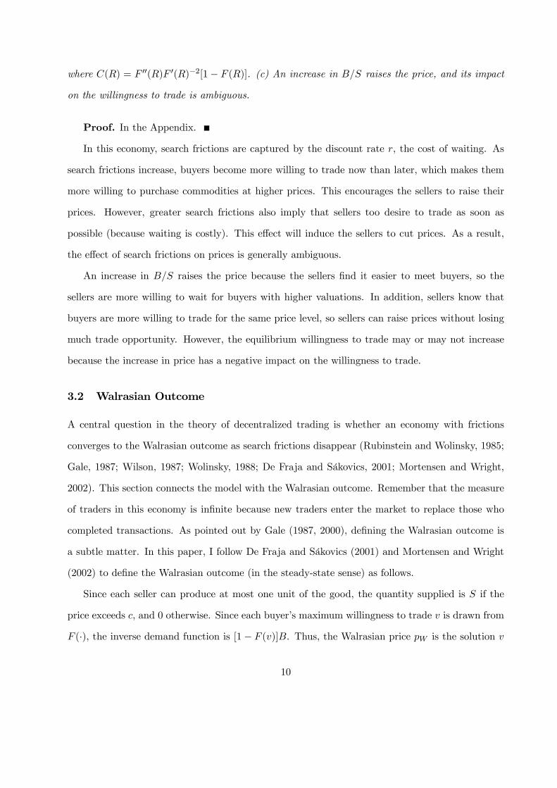
where C(R) = F 00(R)F 0(R)−2[1− F (R)]. (c) An increase in B/S raises the price, and its impacton the willingness to trade is ambiguous.
Proof. In the Appendix.
In this economy, search frictions are captured by the discount rate r, the cost of waiting. As
search frictions increase, buyers become more willing to trade now than later, which makes them
more willing to purchase commodities at higher prices. This encourages the sellers to raise their
prices. However, greater search frictions also imply that sellers too desire to trade as soon as
possible (because waiting is costly). This effect will induce the sellers to cut prices. As a result,
the effect of search frictions on prices is generally ambiguous.
An increase in B/S raises the price because the sellers find it easier to meet buyers, so the
sellers are more willing to wait for buyers with higher valuations. In addition, sellers know that
buyers are more willing to trade for the same price level, so sellers can raise prices without losing
much trade opportunity. However, the equilibrium willingness to trade may or may not increase
because the increase in price has a negative impact on the willingness to trade.
3.2 Walrasian Outcome
A central question in the theory of decentralized trading is whether an economy with frictions
converges to the Walrasian outcome as search frictions disappear (Rubinstein and Wolinsky, 1985;
Gale, 1987; Wilson, 1987; Wolinsky, 1988; De Fraja and Sákovics, 2001; Mortensen and Wright,
2002). This section connects the model with the Walrasian outcome. Remember that the measure
of traders in this economy is infinite because new traders enter the market to replace those who
completed transactions. As pointed out by Gale (1987, 2000), defining the Walrasian outcome is
a subtle matter. In this paper, I follow De Fraja and Sákovics (2001) and Mortensen and Wright
(2002) to define the Walrasian outcome (in the steady-state sense) as follows.
Since each seller can produce at most one unit of the good, the quantity supplied is S if the
price exceeds c, and 0 otherwise. Since each buyer’s maximum willingness to trade v is drawn from
F (·), the inverse demand function is [1− F (v)]B. Thus, the Walrasian price pW is the solution v
10

that satisfies [1− F (v)]B = S for v ≥ c, from which
pW =
F−1
h1− S
B
ifor B ≥ S
c for B < S,
where F−1 is the inverse of F . Note that this definition of the Walrasian price requires market
clearing at each moment, and the short side of the market gets all the trade surplus. Since this
paper is concerned with competition among sellers, unless I state otherwise, I focus on the case
with B < S so that pW = c.
Consider the decentralized economy. Does the equilibrium outcome get closer to the Walrasian
outcome as search frictions disappear?
Proposition 5 In the limit as r → 0, R→ v and
p→ Sc+ 2Bv
S + 2B≡ p∗. (10)
Proof. In the Appendix.
As search frictions disappear, buyers become extremely choosy, and the price posted by the
sellers depends on the relative measure of buyers and sellers. Interestingly, the decentralized
equilibrium does not converge to the Walrasian equilibrium. The intuition for the result is as
follows. Proposition 4 implies that removing search frictions induces both buyers and sellers to be
choosy because there are more opportunities. Buyers will accept less for the same price, and this
induces the sellers to cut their prices. However, the sellers also expect more trade opportunities,
and this induces the sellers to raise their prices. The latter force continues to present even in the
limit because the sellers are the price setters. Thus, sellers do not entirely lose their bargaining
power in the frictionless limit.11 Similarly, the famous Diamond paradox does not arise either
because the buyers’ valuations are unobservable, so buyers do not lose their bargaining power.
Proposition 6 In the limit as B/S → 0, p→ c. In the limit as B/S →∞, p→ v.11The term “bargaining power” is loosely used here even though prices are not negotiable. In this paper, bargaining
power is referred to as the determinant of the division of trade surplus.
11
Proof. In the Appendix.
Instead of removing search frictions, Proposition 6 considers the cases where the relative mea-
sure of sellers is infinite and zero. Even with search frictions and price posting, the decentralized
equilibrium price becomes the unit cost of the product when the relative number of sellers is infinite.
The reason is easily understood. From a buyer’s point of view, the rate at which an acceptable offer
arrives is infinite, so he can be extremely choosy. A seller, on the other hand, faces a ridiculously
small rate of arrival of a buyer, and this drives her bargaining power to zero. The other result is
understood in the same manner.
Finally, it is worth commenting on the implication of free entry. With free entry of sellers, the
measure of sellers S is determined so that Vs = 0 holds. This immediately implies pi = c for all
sellers. This point is somewhat related to the well-known result found in Gale (1987). One of the
keys to obtaining the Walrasian outcome in the frictionless limit of search models is that potential
traders can choose not to enter the market.
4 Discussion
4.1 Ex-Post Bargaining with Observable Valuations
In a related framework, Mortensen and Wright (2002) showed that their decentralized model con-
verges to the Walrasian outcome as frictions disappear. They assumed ex-post bargaining with
observable trade surplus.
Suppose the buyers’ valuations are observable in the model developed in Section 2. With
observable valuations and price setting, no seller has an incentive to set a price ex-ante. The price
is determined ex-post such that the buyer is just indifferent between accepting and rejecting the
trade. This would generate Diamond’s (1971) result.
Now consider a more general case in which the buyer’s valuations are observable and prices are
determined by ex-post bilateral bargaining. I follow Mortensen and Wright (2002) to adopt the
generalized Nash bargaining.12 The total net surplus of a certain pair is given by v− c−Vb−Vs ≡12To be more precise, they adopt a generalized Nash demand game (Osbourne and Rubinstein, 1990), in which
12

Y (v). Thus, the generalized Nash solution requires
pi = (1− β) [c+ Vs] + β [v − Vb] , (11)
where β is the seller’s (exogenous) share of total surplus. Note that pi depends on v. In other
words, with observability of v, the price will be determined conditional on the realization of the
buyer’s valuation. With this pricing rule, the buyer obtains the net surplus of (1−β)Y (v) and the
seller obtains βY (v). Given a meeting, the buyer and seller agree a trade if and only if Y (v) ≥ 0.Let R be the reservation level of v. Thus, the Bellman equations for the buyer and seller are:
rVb = (1 − β)αbR vR[1 − F (v)]dv and rVs = βαs
R vR[1 − F (v)]dv, where R = c + Vb + Vs. Combine
these equations to obtain (R− c)r = [(1−β)αb+βαs]R vR[1−F (v)]dv, which determines the unique
R. The prices are generally dispersed because of the observable valuations and ex-post bargaining.
What happens to the prices as search frictions disappear?
Proposition 7 In the limit as r → 0, R→ v and
p→ (1− β)Sc+ βBv
(1− β)S + βB≡ pb.
Proof. In the Appendix.
It is interesting to observe that although the law of one price is obtained as in Mortensen and
Wright (2002), the price is not Walrasian. According to this expression, the price in the limit equals
the Walrasian (p = c) only if β = 0 or B → 0. In other words, removing search frictions is not
enough to obtain the Walrasian outcome even in the model with observable valuations and ex-post
bargaining. This suggests therefore that the key to the Walrasian outcome in this environment
is the (potential) traders’ exit option that is present in Mortensen and Wright (2002). Since the
model developed in this paper rules out such an option, the model falls into the class of Rubinstein
and Wolinsky (1985) rather than Gale (1987, 2000).
It is interesting to compare the prices p∗ and pb obtained above. It is easy to establish that
p∗ − pb = (2− 3β) q (v − v)(1 + 2q) (1− β + βq)
,
the seller makes a take-it-or-leave-it offer with probability β.
13

where q ≡ B/S. Thus, p∗ ≥ pb holds if and only if β ≤ 2/3. In other words, the price postingwith unobservable valuations amounts to the generalized Nash solution with the seller’s bargaining
power of 2/3.
4.2 Explicit Search Costs
This paper regards the common discount rate r as the (implicit) measure of search frictions.
This interpretation, adopted in many models of decentralized trading, makes sense because the
traders being perfectly patient amounts to saying that the traders make contact with each other
at an infinite rate. However, in the literature of industrial organization with search frictions, it is
common to adopt explicit search costs (Wolinsky, 1986; Stahl, 1989, 1996; Arbatskaya and Konishi,
2005).
Here, I briefly present a model in which the assumption of discounting is replaced with explicit
search costs. The discrete-time versions of the Bellman equations (1) and (3) are
δ = αb
Z Z v
0max v − pi − Vb(p), 0 dF (v)dG(pi), (12)
δ = αs[1− F (R)][pi − c− Vs(pi, p)], (13)
respectively, and all notations should be reinterpreted accordingly. There is no discounting and
traders must pay δ > 0 in each period instead. The reservation utility R is given by R = pi+Vb(p).
Then, (12) reduces to
δ = αb
Z v
R[1− F (v)]dv, (14)
from which it is easy to verify that there is no room for manipulating the acceptability through
prices; R is pinned down by Equation (14).
5 Market Share and Market Power
5.1 Monopoly
In the previous sections, a seller is assumed to ignore how her price will affect the buyers’ willingness
to trade through its impact on their values of search. With this setup, it is evident that the seller
14

faces a trade-off between price and acceptability. However, in equilibrium, higher prices induce the
buyers to be less willing to purchase a commodity because they correctly believe that their values
of search are higher. The key observation is that the failures to take into account the equilibrium
impact of the prevailing price level on the buyers’ values of search are a source of competition in
this environment. If the sellers take into account this effect, will the sellers continue to face the
trade-off between price and acceptability? Will equilibrium exist, and be unique? Will the sellers
set higher prices than when they fail to take into account this effect?
To address the questions above, this section considers an environment in which there is a single
monopolist consisting of a continuum of sellers.13 Note that this is different from an economy with
S → 0, in which a buyer rarely finds a potential trade partner. Here, a buyer can find a seller as
easily as in the previous economy, but it is impossible to find competing sellers. In addition, the
monopolist takes into account how the price influences the buyers’ values of search because the
monopolist regards the equilibrium price and each seller’s price as the same thing.
In this economy, a buyer’s value satisfies
rVb(p) = αb
Z v
0max v − p− Vb(p), 0 dF (v).
Note that from the buyer’s perspective, all sellers are the same.14 The reservation strategy is to
accept a trade if and only if v ≥ R, where R = p+ Vb(p). Given the reservation strategy, it is easyto rewrite the buyer’s value as rVb(p) = αb
R vR[1− F (v)]dv. Substitute it back into R = p+ Vb(p)
to obtain the equilibrium relationship between p and R: p = R − (αb/r)R vR[1 − F (v)]dv ≡ H(R),
which is identical to (8).
Consider the firm. The value of posting p is given by rVs (p) = αs[1 − F (R)][p − c − Vs (p)].The firm chooses p to maximize the value of search, taking into account the buyer’s equilibrium
reservation strategy. To be precise, the firm’s problem is: maxp Vs(p) subject to p = H(R).
13Early contributions on monopoly pricing with search frictions are found in Albrecht and Jovanovic (1986) and
Wang (1995).14This is the consequence of the buyers’ beliefs that no seller will deviate from what the firm has decided. In this
sense, it will be helpful to regard each seller as a vending machine.
15

Proposition 8 The firm posts
p = c+[1− F (R)] + (αs/r)[1− F (R)]2
F 0(R)H 0(R) ≡M(R). (15)
Proof. In the Appendix.
Lemma 9 M(R) is decreasing if the distribution function satisfies (6).
Proof. In the Appendix.
A steady-state equilibrium with monopoly pricing is a set of posted price p and reservation
utility R that satisfies p = H(R) and p = M(R). Then the price posting curve is downward
sloping, and there is a unique steady state equilibrium. Since H 0(R) > 1, it is easy to verify that
M(R) > P (R) holds for all R, as depicted in Figure 2. In this equilibrium, the price is higher and
the buyers are choosier than in the model with a continuum of negligible sellers.
From a seller’s perspective, if a buyer walks away, then this buyer will trade with someone else
for sure. Thus, sellers become “myopic” (Reinganum, 1982). This introduces some competition
among sellers, and a seller has an incentive to reduce the price. On the other hand, in the monopoly
case, all sellers belong to a single firm, and the firm knows that even though a buyer walks away
from a particular seller, this buyer will have to trade with another seller from the same firm. This
gives the firm more bargaining power, leading to a higher price. However, the buyers do not entirely
lose their bargaining power because their valuations are unobservable and they always have the
options to postpone consumption.
5.2 Oligopoly
An important issue in price theory is to explain the Bertrand Paradox and the Diamond Paradox.
The former states that two firms are enough to generate the perfectly competitive outcome in
the Bertrand price competition model. The latter states that even with a large number of firms,
there will be no price competition among firms as long as each buyer faces a small search cost. As
pointed out by Gale (1988), the difference in the two models is, in principle, the order of play: in
the former, buyers choose which store to go to after observing the prices; in the latter, buyers visit
16

sellers before their prices are quoted. The question addressed in this section is therefore as follows.
If there is a finite (countable) number of firms in this decentralized economy with search frictions,
how competitive will the prices be?
Suppose there are N firms, each consisting of a continuum of sellers. Each firm is considered
to be a coalition of sellers that pools the values of all members, and it sets the price on behalf of
the members.15 Let j = 1, ..., N index each firm. The basic idea behind this formulation is that
the market power of a certain firm is captured by the size of the coalition; as the size of coalition
approaches 1, the firm becomes more monopolistic (in the sense of the model in the previous
section). The fraction of sellers belonging to firm j is denoted by θj , and is conveniently referred
to as the “market share” or the degree of dominance. Evidently,PNj=1 θj = 1. I assume that all
sellers of firm j follow the same strategy and therefore set the same price pj .
Consider a buyer’s decision. A buyer meets a seller with probability αb, and this seller happens
to belong to firm j with probability θj . The buyer observes v, and agrees to a trade if and only if
the gains from the trade exceed the value of continuing the search. Thus, the value of search Vb
satisfies
rVb(p1, ..., pN ) = αb
NXj=1
θj
Z v
0max v − pj − Vb(p1, ..., pN), 0 dF (v).
The buyer accepts a trade if and only if v ≥ Rj holds, where Rj = pj + Vb(p1, ..., pN). In other
words, the buyer forms a reservation utility for each firm. Given these reservation strategies,
Vb(p1, ..., pN) =αbr
NXj=1
θj
Z v
Rj
[1− F (v)] dv ≡ Ω (R1, ..., RN ) .
Substitute this back into the cutoff condition to obtain
pj = Rj − Ω(R1, ..., RN) (16)
for j = 1, ..., N . This summarizes the trade-off that each firm faces. It is easy to show that
∂pj/∂Rj = 1+(αb/r)θj [1−F (Rj)] < H 0(Rj) because θj ∈ (0, 1). This implies that an oligopolisticfirm internalizes partially the effect of a price change on the equilibrium price.15As in the previous section, it is appropriate to regard each seller as a vending machine. The idea that each trader
belongs to a coalition in a search environment first appears in Shi (1997). In Shi (1998), prices are determined in a
decentralized manner.
17

The value of a seller belonging to firm j satisfies
rV js (pj) = αs[1− F (Rj)][pj − c− V js (pj)]. (17)
Thus, the pricing problem for firm j is maxpj Vjs (pj) subject to (16), taking all other firms’ prices
as given.
Proposition 10 Each firm j (j = 1, ..., N) posts
pj = c+[1− F (Rj)] + (αs/r)[1− F (Rj)]2
F 0(Rj)[1 + (αb/r)θj [1− F (Rj)]] ≡ Lj (Rj) . (18)
The problem can be solved similarly as in Proposition 8. H 0(R) in (15) is replaced with 1 +
(αb/r)θj [1−F (Rj)], which captures the degree of market power: if θj = 0 then the pricing behaviorcoincides with a single (infinitesimal) seller in the basic model; if θj = 1 then this corresponds to
the monopoly case. From (18), it is easy to show that ∂pj/∂θj > 0, which suggests that larger
firms (in terms of the market share) have incentives to set higher prices.
Market equilibrium is defined as a set of prices and reservation strategies such that (16) and (18)
are satisfied. Consider the symmetric equilibrium in which all firms have the same size (θj = S/N
for all j). As N → ∞, the equilibrium approaches the one with a continuum of negligible sellers.
As N → S, the equilibrium approaches the one with a monopolist.
In what follows, I focus on the duopoly case (N = 2). An equilibrium is given by pj =
Rj − Ω(R1, R2) and pj = Lj (Rj) for j = 1, 2. From (16),
p1 − p2 = R1 −R2, (19)
which implies p1 > p2 ⇔ R1 > R2. Since Lj (Rj) is monotone-decreasing, pj = Lj (Rj) implies
Rj = L−1j (pj), where L
−1j is the inverse of Lj . Substitute this into the other equation to obtain
p1 = L−11 (p1)− Ω(L−11 (p1), L−12 (p2)), (20)
p2 = L−12 (p2)− Ω(L−11 (p1), L−12 (p2)). (21)
The equilibrium is given by a pair (p1, p2) that solves (20) and (21). These expressions implicitly
define p1 = µ1(p2) and p2 = µ2(p1), from which it is possible to show the following:
18

Lemma 11 µ01(p2) < 0 and µ02(p1) < 0.
Proof. In the Appendix.
It is now evident that the firms’ actions are strategic substitutes. The intuition for the result is
as follows. Suppose firm 1 reduces its price. The direct effect is that buyers become more willing
to purchase from sellers of firm 1. The indirect effect is that a decrease in p1 increases the buyers’
values of search. This makes the buyers less willing to purchase from sellers of both firms. Firm
2’s optimal reaction to this is to raise the price slightly to offset the increase in the buyers’ values
of search.
Proposition 12 An increase in the size of a firm raises its price and reduces the rival’s price.
Proof. In the Appendix.
Corollary 13 There is price dispersion unless θ1 = θ2 = 1/2.
As a firm gets larger, its market power increases and it sets a higher price than its rival
firm. Accordingly, two different prices are possible in the search equilibrium. This suggests a new
explanation for price dispersion, namely, search frictions combined with oligopolistic competition.
Interestingly, the property of the equilibrium is closer to the one of the Cournot model than that
of the Bertrand model, even though the firms compete by choosing their prices. An important
lesson here is that price competition per se is not the key. Rather, as clarified by Gale (1988), what
matters is whether the buyers can choose which firm to go to after the prices are quoted.
6 Conclusion
This paper developed a simple random search model with price posting in which the sellers face a
trade-off between price and the buyer’s willingness to trade, and the trade-off is derived naturally
from the basics of the model. The trade-off between price and the willingness to trade has not been
observed in the consumer search models without discounting. In this sense, the trade-off found
in this paper is dynamic in nature. To demonstrate the usefulness of the model, monopoly and
19
oligopoly have been studied. It has been shown that price dispersion arises as a result of search
frictions and price setting, and this is new to the literature.
This paper has focused on a stationary equilibrium by assuming that a buyer who completed a
transaction is replaced with a clone. Although this is a fairly standard assumption in search theory,
it introduces some nontrivial implications into the analysis. One is that the framework becomes
non-Walrasian even in the limit as search frictions disappear. Another important implication is
that supply creates its own demand in the sense that if sellers cut prices then they can expect
the aggregate demand to increase without reducing the future demand. In other words, there
is assumed to be no intertemporal trade-off of demands. A possible extension of this analysis
is to consider a nonstationary environment in the spirit of Fershtman and Fishman (1992) so as
to introduce the mechanism where the future aggregate demand decreases if the buyers’ current
consumptions are high.
This paper has maintained the assumption of random search. As stated briefly in the Intro-
duction, an important development has been observed in the field of directed search theory, which
is by construction more competitive than a random search environment. It will be worthwhile to
explore whether the Cournot outcome continues to hold in the duopoly model with directed search
using the model developed in this paper.
20

Appendix
A Proof of Proposition 1
The first-order condition for the maximization problem of the right-hand side (4) is given by
αs[1− F (R)][1− ∂Vs(pi, p)/∂pi]− αsF0(R)[pi − c− Vs(pi, p)] = 0. The Envelope Theorem implies
∂Vs(pi, p)/∂pi = 0, so
[1− F (R)] = F 0 (R) [pi − c− Vs(pi, p)]. (22)
Solve (3) for Vs and substitute it into (22) to obtain the price pi as a function of R. The second-
order condition is −2F 0(R)−F 00(R)[pi− c−Vs(pi, p)] < 0. Use the first-order condition to rewriteit as C(R) < 2, where C(R) = F 00(R)F 0(R)−2[1−F (R)]. To verify that this function is decreasing,differentiate (5) to obtain
P 0(R) = − [1 + (αs/r)[1− F (R)]] [1 + C(R)]− (αs/r)[1− F (R)]. (23)
Thus, it is evident that a sufficient condition for the existence of decreasing P (R) is −1 < C(R) < 2.
B Proof of Proposition 3
Lemma 2 establishes that H(R) is increasing. From Proposition 1, P (R) is decreasing if (6) holds.
From (8) and (5), P (0) > H(0) because c + [1 + (αs/r)]F 0(0)−1 > −(αb/r)R v0 [1 − F (v)]dv holds
for F 0(0) ≥ 0. That is, P (0) > H(0) holds under any density F 0(v) > 0. Finally, P (v) −H(v) =c+ 0/F 0(v)− v < 0 holds if F 0(v) > 0 and c < v. The term 0/F 0(v) is not well-defined in the case
of F 0(v) = 0. Applying l’Hopital’s rule, it is easy to verify that
P (v)−H(v) = c+ limR→v
−F 0(R)− 2(αs/r)[1− F (R)]F 00(R)F 00(R)
− v = c− v < 0.
This establishes the existence and uniqueness of equilibrium under the maintained assumptions
c < v and (6).
21

C Proof of Proposition 4
From (5), ∂P/∂r = −αs[1 − F (R)]2/[r2F 0(R)] < 0 and P 0(R) is given by (23). Similarly, from
(8),∂H/∂r = (αb/r2)R vR[1−F (v)]dv > 0 and H 0(R) = 1+ (αb/r)[1−F (R)] > 0. (a) From (5) and
(8), it is easy to verify that an increase in r will shift the p = P (R) locus downward and p = H(R)
locus upward in Figure 1. Thus, R will unambiguously decrease. (b) Totally differentiate (5) and
(8) to obtain dp = P 0(R)dR+ [∂P (R)/∂r]dr and dp = H 0(R)dR+ [∂H(R)/∂r]dr. Thus,·1− P
0(R)H 0(R)
¸dp
dr=
∂P (R)
∂r− P
0(R)H 0(R)
∂H(R)
∂r.
Since P 0(R) < 0 < H 0(R), the left-hand side of this expression is positive. Thus, dp/dr > 0 holds
if and only if its right-hand side is positive, or [∂P (R)/∂r]/[∂H(R)/∂r] > P 0(R)/H 0(R), or
−[1− F (R)]2F 0 (R)
R vR[1− F (v)]dv
>αbαs
− [r + αs[1− F (R)]] [1 + C(R)]− αs[1− F (R)]r + αb[1− F (R)] .
Thus, the effect is ambiguous. (c) Let q ≡ B/S for convenience. From (5) and (8), it is easy to
obtain∂P
∂q=[1− F (R)]2rF 0 (R)
∂αs∂q
> 0,∂H
∂q= −1
r
µZ v
R[1− F (v)]dv
¶∂αb∂q
> 0.
From Figure 1 it is easy to establish that dp/dq > 0. Totally differentiate (5) and (8) to obtain
[P 0(R)−H 0(R)]dR/dq = ∂H(R)/∂q−∂P (R)/∂q. Since P 0(R)−H 0(R) < 0, dR/dq > 0 if and only
if
−µZ v
R[1− F (v)]dv
¶∂αb∂q
<[1− F (R)]2F 0 (R)
∂αs∂q.
Thus, the effect is ambiguous.
D Proof of Proposition 5
From (7), Vb = (αb/r)R vR[1−F (v)]dv. Since Vb is bounded, as r → 0,
R vR[1−F (v)]dv must converge
to zero. This implies R→ v ad r→ 0. In what follows I denote R = R(r). Consider (5). Take the
limit on the right-hand side:
limr→0P (R) = c+
1− F (v)F 0 (v)
+ limr→0
αs[1− F (R(r))]2rF 0 (R(r))
. (24)
22

Since F 0 (v) > 0, the second term on the right-hand side of (24) is zero. Apply l’Hopital’s rule to
the third term and obtain
limr→0P (R(r)) = c+ αs lim
r→0
(−2[1− F (R(r))][F 0(R(r))]2 − [1− F (R(r))]2F 00(R(r))
[F 0 (R(r))]2R0(r)
)= c− αs lim
r→0 [2 + C(R(r))] [1− F (R(r))]R0(r),
where C(R) = F 00(R)[1− F (R)]/F 0(R)2 > −1 and R0(r) < 0. Similarly, from (8),
limr→0H(R(r)) = v − αb lim
r→0
R vR(r)[1− F (v)]dv
r= v − αb lim
r→0−[1− F (R(r))]R0(r)
1.
Thus, the posted price in the limit, denoted by p∗, satisfies
p∗ = c− αs limr→0 [2 + C(R(r))] [1− F (R(r))]R
0(r), (25)
p∗ = v + αb limr→0[1− F (R(r))]R
0(r). (26)
Suppose that limr→0[1 − F (R(r))]R0(r) = 0. Then (25) and (26) imply p∗ = c and p∗ = v,
a contradiction. Similarly, it cannot be −∞. Thus, [1 − F (R(r))]R0(r) must converge to somenumber k ∈ (−∞, 0). Note that limr→0 [2 + C(R(r))] = 2. With convergence, (25) may be writtenas p∗ = c−αs limr→0[2+C(R(r))] limr→0[1−F (R(r))]R0(r). Thus, p∗ must satisfy p∗ = c−αs2k =c− qαb2k and p∗ = v + αbk. Eliminate k from these expressions to obtain the desired result.
E Proof of Proposition 6
Note that as B/S → 0, αb → ∞ and αs → 0. From (7), Vb = (αb/r)R vR[1 − F (v)]dv. Since Vb is
bounded, as αb →∞,R vR[1− F (v)]dv must converge to zero. This implies R→ v. From (5)
pi → c+1− F (v)F 0 (v)
= c.
Similarly, as B/S →∞, αb → 0 and αs →∞. Then, (7) implies that Vb → 0 and R→ pi. In other
words, a buyer will accept a trade if the value of the good exceeds its price. Since the seller’s value
of search must be bounded, (3) implies that as αs →∞, pi → v. In other words, each seller posts
the price at the buyer’s maximum willingness to pay, since the seller faces no frictions in this limit.
23

F Proof of Proposition 7
The equilibrium is characterized by rVb = (1− β)αbR vR [1− F (v)] dv, rVs = βαs
R vR [1− F (v)] dv,
and (R − c)r = [(1 − β)αb + βαs]R vR[1 − F (v)]dv. It is evident from the Bellman equations that
as r → 0, R→ v. That is, traders become extremely choosy. Thus, trades are possible only when
v = v, implying from (11) that there will be no price dispersion. Let (1/r)R vR [1− F (v)] dv ≡ K
and eliminate K from the expressions above to obtain
limr→0Vb =
(1− β)αb (v − c)(1− β)αb + βαs
, limr→0Vs =
βαs (v − c)(1− β)αb + βαs
.
Substitute these into (11) to obtain
limr→0 pi =
c (1− β)αb + βvαs(1− β)αb + βαs
=c (1− β)S + βvB
(1− β)S + βB.
G Proof of Proposition 8
The Lagrangian for this problem is αs[1 − F (R)][p − c − Vs (p)] + λ[H(R) − p], where λ is the
Lagrangian multiplier. The first-order conditions with respect to p and R are αs[1 − F (R)][1 −V 0s (p)] = λ and αsF
0(R)[p− c− Vs (p)] = λH 0(R), respectively. Thus,
F 0 (R)1− F (R) [p− c− Vs (p)] = H
0(R). (27)
Solve rVs (p) = αs[1− F (R)][p− c− Vs (p)] for Vs(p) and substitute it into (27) to obtainF 0 (R)1− F (R)
r (p− c)r + αs[1− F (R)] = H
0(R).
Solve this equation for p to obtain the desired result.
H Proof of Lemma 9
Consider p =M(R) = c+T (R)H 0(R), where T (R) ≡ [1−F (R)]+(αs/r)[1−F (R)]2/F 0(R) > 0.Since M 0(R) = T 0(R)H 0(R) + T (R)H 00(R), Lemma 2 implies that M 0(R) < 0 holds if T 0(R) < 0.
From the argument in Proposition 1, a sufficient condition for T 0(R) < 0 is −[1−F (R)]−1[F 0(R)]2 <F 00(R).
24

I Proof of Lemma 11
The steady-state equilibrium is characterized by (20) and (21). To be more precise,
p1 = L−11 (p1)−αbrθ1
Z v
L−11 (p1)[1− F (v)] dv − αb
rθ2
Z v
L−12 (p2)[1− F (v)] dv,
p2 = L−12 (p2)−αbrθ1
Z v
L−11 (p1)[1− F (v)] dv − αb
rθ2
Z v
L−12 (p2)[1− F (v)] dv.
Totally differentiate these equations to obtain
dp1dp2
=
αbr θ2
h1− F (L−12 (p2))
i∂L−12 (p2)
∂p2
1−n1 + αb
r θ1h1− F (L−11 (p1))
io∂L−11 (p1)
∂p1
,
dp2dp1
=
αbr θ1
h1− F (L−11 (p1))
i∂L−11 (p1)
∂p1
1−n1 + αb
r θ2h1− F (L−12 (p2))
io∂L−12 (p2)
∂p2
,
where∂L−11 (p1)
∂p1=
1
L01(L−11 (p1))
< 0,∂L−12 (p2)
∂p2=
1
L02(L−12 (p2))
< 0.
Thus, dp1/dp2 < 0 and dp2/dp1 < 0.
J Proof of Proposition 12
Instead of working directly with prices, I shall work with R1 and R2. Then the equilibrium is
characterized by a pair (R1, R2) such that
Rj − αbrθ1
Z v
R1[1− F (v)] dv − αb
r(1− θ1)
Z v
R2[1− F (v)] dv
= c+ P (Rj) [1 + (αb/r)θj [1− F (Rj)]]
for j = 1, 2, where
P (Rj) =[1− F (Rj)] + (αs/r)[1− F (Rj)]2
F 0(Rj)= P (Rj)− c, P 0(Rj) < 0.
Totally differentiate these expressions and arrange terms to obtain
αbr(1− θ1) [1− F (R2)] dR2 = P 0(R1) [1 + (αb/r)θ1[1− F (R1)]] dR1
−P (R1)(αb/r)θ1F 0(R1)dR1 − dR1 − αbrθ1 [1− F (R1)] dR1
+P (R1)(αb/r)[1− F (R1)]dθ1 + αbr
Z R2
R1[1− F (v)] dvdθ1,
25
and
αbrθ1 [1− F (R1)] dR1 = P 0(R2) [1 + (αb/r) (1− θ1) [1− F (R2)]] dR2
−P (R2)(αb/r) (1− θ1)F0(R2)dR2 − dR2 − αb
r(1− θ1) [1− F (R2)] dR2
−P (R2)(αb/r)[1− F (R2)]dθ1 + αbr
Z R2
R1[1− F (v)] dvdθ1,
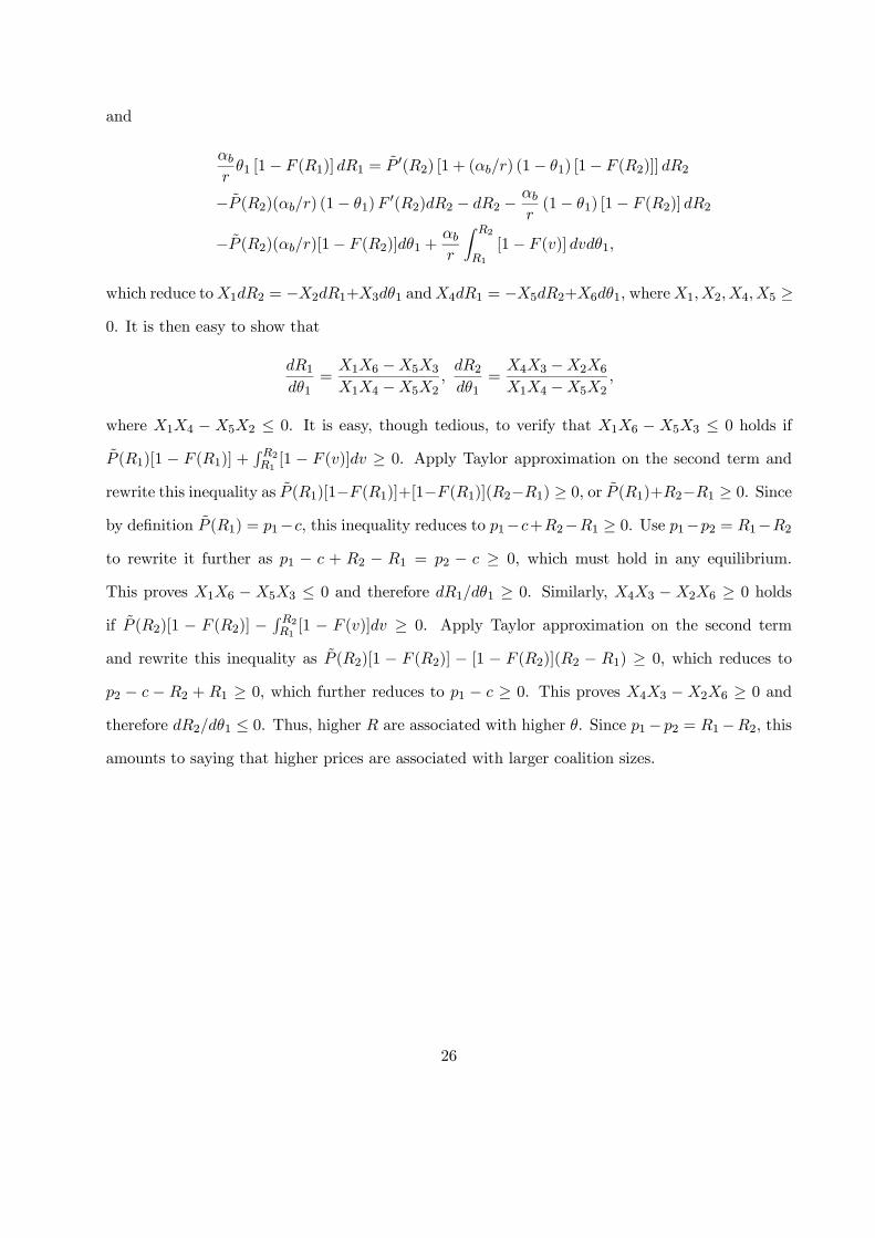
which reduce toX1dR2 = −X2dR1+X3dθ1 andX4dR1 = −X5dR2+X6dθ1, whereX1,X2,X4,X5 ≥0. It is then easy to show that
dR1dθ1
=X1X6 −X5X3X1X4 −X5X2 ,
dR2dθ1
=X4X3 −X2X6X1X4 −X5X2 ,
where X1X4 − X5X2 ≤ 0. It is easy, though tedious, to verify that X1X6 − X5X3 ≤ 0 holds ifP (R1)[1 − F (R1)] +
RR2R1[1 − F (v)]dv ≥ 0. Apply Taylor approximation on the second term and
rewrite this inequality as P (R1)[1−F (R1)]+[1−F (R1)](R2−R1) ≥ 0, or P (R1)+R2−R1 ≥ 0. Sinceby definition P (R1) = p1−c, this inequality reduces to p1−c+R2−R1 ≥ 0. Use p1−p2 = R1−R2to rewrite it further as p1 − c + R2 − R1 = p2 − c ≥ 0, which must hold in any equilibrium.
This proves X1X6 − X5X3 ≤ 0 and therefore dR1/dθ1 ≥ 0. Similarly, X4X3 − X2X6 ≥ 0 holdsif P (R2)[1 − F (R2)] −
R R2R1[1 − F (v)]dv ≥ 0. Apply Taylor approximation on the second term
and rewrite this inequality as P (R2)[1 − F (R2)] − [1 − F (R2)](R2 − R1) ≥ 0, which reduces top2 − c − R2 + R1 ≥ 0, which further reduces to p1 − c ≥ 0. This proves X4X3 − X2X6 ≥ 0 andtherefore dR2/dθ1 ≤ 0. Thus, higher R are associated with higher θ. Since p1− p2 = R1−R2, thisamounts to saying that higher prices are associated with larger coalition sizes.
26

References
[1] Acemoglu, Daron, and Robert Shimer. “Holdups and Efficiency with Search Frictions”, Inter-
national Economic Review 40 (1999) 827—849.
[2] Albrecht, James, and Boyan Jovanovic. “The Efficiency of Search under Competition and
Monopsony”, Journal of Political Economy 94 (1986) 1246—1257.
[3] Arbatskaya, Maria, and Hideo Konishi. “Referrals in Search Markets,” mimeo, 2005.
[4] Bagnoli, Mark, and Ted Bergstrom. “Log-concave Probability and Its Applications”, Economic
Theory 26 (2005) 445—469.
[5] Bester, Helmut. “Price Commitment in Search Markets”, Journal of Economic Behavior and
Organization 25 (1994) 109—120.
[6] Burdett, Kenneth, and Randall Wright. “Two-Sided Search with Nontransferable Utility”,
Review of Economic Dynamics 1 (1998) 220—45.
[7] Curtis, Elisabeth, and Randall Wright. “Price Setting, Price Dispersion, and the Value of
Money: or, the Law of Two Prices”, Journal of Monetary Economics 51 (2004) 1599—1621.
[8] De Fraja, Gianni, and József Sákovics. “Walras Retrouvé: Decentralized Trading Mechanisms
and the Competitive Price”, Journal of Political Economy 109 (2001) 842—863.
[9] Diamond, Peter A. “A Model of Price Adjustment”, Journal of Economic Theory 3 (1971)
156—168.
[10] Fershtman, Chaim, and Arthur Fishman. “Price Cycles and Booms: Dynamic Search Equi-
librium”, American Economic Review 82 (1992) 1221—1233.
[11] Gale, Douglas. “Limit Theorems for Markets with Sequential Bargaining”, Journal of Eco-
nomic Theory 43 (1987) 20—54.
27

[12] Gale, Douglas. “Price Setting and Competition in a Simple Duopoly Model”, Quarterly Jour-
nal of Economics 103 (1988) 729—739.
[13] Gale, Douglas. Strategic Foundations of General Equilibrium: Dynamic Matching and Bar-
gaining Games, Cambridge University Press, Cambridge, 2000.
[14] Masters, Adrian M. “Wage Posting in Two-Sided Search and the Minimum Wage”, Interna-
tional Economic Review 40 (1999) 809—26.
[15] Mortensen, Dale T. and Randall Wright. “Competitive Pricing and Efficiency in Search Equi-
librium”, International Economic Review 43 (2002) 1—20.
[16] Osborne, Martin J., and Ariel Rubinstein. Bargaining and Markets. Academic Press, San
Diego, 1990.
[17] Reingnum, Jennifer F. “Strategic Search Theory”, International Economic Review 23 (1982)
1—17.
[18] Rogerson, Richard, Robert Shimer, and Randall Wright. “Search-Theoretic Models of the
Labor Market: A Survey,” Journal of Economic Literature 18 (2005) 959—988.
[19] Rubinstein, Ariel, and Asher Wolinsky. “Equilibrium in a Market with Sequential Bargaining”,
Econometrica 53 (1985) 1133—1150.
[20] Shi, Shouyong. “A Divisible Search Model of Fiat Money,” Econometrica 65 (1997) 75—102.
[21] Stahl, Dale O. “Oligopolistic Pricing with Sequential Consumer Search”, American Economic
Review 79 (1989) 700—712.
[22] Stahl, Dale O. “Oligopolistic Pricing with Heterogeneous Consumer Search”, International
Journal of Industrial Organization 14 (1996) 243—268.
[23] Wang, Ruqu. “Bargaining versus Posted-price Selling”, European Economic Review 39 (1995)
1747—1764.
28

[24] Wilson, Robert. “Game-theoretic Analyses of Trading Processes”, in, Truman F. Bewley (edi-
tor) Advances in Economic Theory: Fifth World Congress, Cambridge University Press, Cam-
bridge, 1987.
[25] Wolinsky, Asher. “True Monopolistic Competition as a Result of Imperfect Information”,
Quarterly Journal of Economics 101 (1986) 493—512.
[26] Wolinsky, Asher. “Dynamic Markets with Competitive Bidding”, Review of Economic Studies
55 (1988) 71—84.
29

Figure 1
)(RH
)(RP
R
p
Figure 2
)(RP)(RM
)(RH
R
p
c