Parent-Child Information Frictions and Human Capital Investment:Evidence from a Field Experiment∗

Peter Bergman†

This paper uses a field experiment to answer how information frictions between parentsand their children affect human capital investment and how much reducing these frictionscan improve student achievement. A random sample of parents was provided additionalinformation about their child’s missing assignments, grades and upcoming exams. As ina standard principal-agent model, more information allowed parents to induce more effortfrom their children, which translated into gains in achievement. Importantly however, ad-ditional information also changed parents’ beliefs and spurred demand for information fromthe school. Relative to other interventions, additional information to parents potentiallyproduces gains in achievement at a low cost.

JEL Codes: I20, I21, I24.

∗I am extremely grateful to Adriana Lleras-Muney, Pascaline Dupas and Karen Quartz fortheir advice and support. I thank Sandra Black, Jon Guryan, Day Manoli and Sarah Reberfor their detailed feedback. I also thank seminar participants at Case Western University,the CFPB, Mathematica, RAND, UC Berkeley, the University of Chicago Becker FriedmanInstitute and UCLA for their comments and suggestions. All errors are my own.†Economics Department, UCLA 8283 Bunche Hall, Los Angeles CA 90095 E-mail:

peterlsb@ucla.edu.

I Introduction

When asked what would improve education in the United States the most, Americans cite

more parental involvement twice as often as anything else (Time, 2010). Numerous papers

reinforce the importance of parental investments in their child’s human capital (e.g. Cunha

et al., 2006; Houtenville and Smith Conway, 2007; Todd and Wolpin, 2007). However, if

children hide information about their academic progress from their parents, a principal-agent

problem might arise that impedes these investments. Providing parents more information

about their child’s academic progress is potentially a cost-effective way to increase student

effort and to improve academic outcomes. This paper uses a field experiment to answer how

information frictions impede parental investments and if reducing these frictions can improve

student effort and achievement.

At the outset it is uncertain whether additional information to parents can improve out-

comes. There is an association between the quality of information schools provide and school

performance: In schools where most students go on to college, 83% of parents are satisfied

with the school’s ability to communicate information about their child’s academic perfor-

mance, but in schools where most students do not go on to college, 43% of the parents are

satisfied with this communication (Civic Enterprises, 2004). However it is not clear what

underlies this association. Parents of students who are performing well might be receiving

better information or they might require less information because their children have greater

academic ability. Even if more information does increase parental investment in their child’s

education, it is not obvious this will improve academic outcomes. More information might

help parents induce more effort from their children, but complementary inputs of the educa-

tion production function, such as teacher instruction, also determine if this effort translates

into measurable gains in achievement.

To measure the causal effect of additional information on parents’ investments in their

children and student outcomes, I conducted an experiment at a low-performing school near

downtown Los Angeles. Out of all 462 students in grades six through eleven, 242 students’

parents or guardians were randomly selected to receive additional information about their

child’s academic progress. This information consisted of emails, text messages and phone

calls listing students’ missing assignments and grades several times a month over a six-month

period. The information provided was detailed. Messages contained the class, assignment

names, problems and page numbers of the missing work whenever possible. Course grades

were sent to families every five to eight weeks.1 To quantify the effects on student effort,

achievement and parental investments, I gathered administrative data on assignment com-

1This is in addition to the report cards sent by mail to all families in the treatment and control groups.

1

pletion, work habits, cooperation, attendance and test scores. Parent and student surveys

were conducted immediately after the school year ended to provide additional data about

each family’s response.

The results for high school students suggest there are significant information frictions be-

tween parents and their children. As in a standard principal-agent model, more information

increased the intensity of parents’ incentives and improved their child’s effort. Importantly

however, some parents were not fully aware of these frictions. Parents in the high school

treatment group were twice as likely as the control group to believe that their child does not

tell them enough about their schoolwork and grades. This change in beliefs coincides with

an increase in parents’ demand for information from the school about their child’s academic

progress. Parents in the treatment group contacted the school about this information 83%

more often than the control group, and parent-teacher conference attendance increased by

53%. Unfortunately, the middle-school teachers replicated the treatment for all students in

their grades, contaminating the results for those families. There was no estimated effect on

middle school parent or student outcomes.

In terms of achievement, additional information potentially can produce gains on par

with education reforms such as high-quality charter schools. For high school students, GPA

increased by .21 standard deviations. There is evidence that test scores for math increased

by .21 standard deviations, though there was no gain for English scores (.04 standard devia-

tions). These effects are driven by a 25% increase in assignment completion and a 24% and

25% decrease in the likelihood of unsatisfactory work habits and cooperation, respectively.

Classes missed by students decreased by 28%. For comparison, the Harlem Children’s Zone

increased math scores and English scores by .23 and .05 standard deviations and KIPP Lynn

charter schools increased these scores .35 and .12 standard deviations (Dobbie and Fryer,

2010; Angrist et al., 2010).

Relative to other interventions, providing information could be a cost effective way to

address sub-optimal student effort and reduce the achievement gap.2 Interventions aimed at

adolescents’ achievement are often costly because they rely on financial incentives, either for

teachers (Springer et al., 2010; Fryer, 2011), for students (Angrist and Lavy, 2002; Bettinger,

2008; Fryer, 2011) or for parents (Miller, Riccio and Smith, 2010). Providing financial

incentives for high school students cost $538 per .10 standard-deviation increase, excluding

administrative costs (Fryer, 2011). If teachers were to provide additional information to

parents as in this study, the cost per student per .10 standard-deviation increase in GPA or

2Examples of other information-based interventions in education include providing families information describing studentachievement at surrounding schools (Hastings and Weinstein, 2008; Andrabi, Das and Khwaja 2009), parent outreach programs(Avvisati et al., 2010), providing principals information on teacher effectiveness (Rockoff et al., 2010) and helping parents fillout financial aid forms (Bettinger et al., 2009).

2

math scores would be $156 per child per year. Automated messages could reduce this cost

further.

These costs raise an important related question, which is how much parents might be

willing to pay to reduce these information problems. This study does not address this

question, but Bursztyn and Coffman (2011) use a lab experiment with low-income families

in Brazil to show parents are willing to pay substantial amounts of money for information

on their child’s attendance.

While this paper shows that an intensive information-to-parents service potentially can

produce gains to student effort and achievement, its policy relevance depends on how well

it translates to other contexts and scales up. Large school districts such as Los Angeles,

Chicago, and San Diego have purchased systems that make it easier for teachers to improve

communication with parents by posting grades online, sending automated emails regarding

grades, or text messaging parents regarding schoolwork. The availability of these services

prompts questions about their usage, whether teachers update their grade books often enough

to provide information, and parental demand for this information. This paper discusses but

does not address these questions empirically.

The rest of the paper proceeds as follows. Sections II and III describe the experimental

design and the estimation strategy. Sections IV and V present the results for the high school

students and middle school students, respectively. Section VI concludes with a discussion of

external validity and cost-effectiveness.

Section II outlines a basic framework to interpret the empirical analysis.

II Framework

Typically, models of human capital investment do not incorporate information frictions be-

tween parents and their children.3 Students may wish to hide information from their parents

about their human capital investment due to higher discount rates or difficulty planning for

the future (Bettinger and Slonim, 2007; Steinberg et al., 2009; Levitt, List, Neckermann and

Sadoff, 2011).

The framework below posits a simple non-cooperative interaction between parents and

their children to show how additional information can affect student achievement. Student

achievement A is a function of student effort e and teacher quality T . Effort e is also

a function of a vector z and a vector of parental investments I. z includes a student’s

ability, peers, discount rate, and value of education. A child takes I as given and maximizes

3Several important exceptions in the context of human-capital investment are Weinberg (2001), Berry (2009), and Bursztynand Coffman (2011).

3

maxe {u(A(e; I, z, T ))− e}. Solving, the best response to I is e(I, z, T ).

Parents choose I at a cost of c(I; ε, t). The cost function represents, in a reduced form, the

cost of parental monitoring, helping with schoolwork directly, or providing incentives. The

vector ε captures parental heterogeneity such as their value of education, work schedule,

and parenting skills. t is an indicator variable for receiving the information treatment.

Parents take their child’s best response as given and maximize the utility they get from their

achievement (normalized to A): A(e(I; z, T ))− c(I; ε, t). The first-order condition yields

∂A(e(I; z, T ))

∂e× ∂e(I; z, T )

∂I=∂c(I; ε, t)

∂I(1)

The right-hand side of equation (1) is the marginal cost of parents’ investments. The

information treatment t could reduce this marginal cost, for instance, by lowering monitoring

costs for parents. In a standard moral hazard problem, this lower monitoring cost could

increase the intensity of incentives, and in turn, improve student effort. I examine this

implication using survey and administrative data.

Equation (1) also highlights several complementarities. The treatment effect depends on

parents’ valuation of education (part of ε). Parents who place little value on education are

likely to ignore information regarding their child’s academic progress. Even if the implication

of the standard principal-agent model holds such that investment increases and student effort

increases (∂e(I; z, T )/∂I > 0), this does not imply a positive effect on student achievement,

which depends on the quality of teacher inputs T in the achievement function. If teachers

provide students work that is either unproductive or that does not translate into higher test

scores, then there will be no measured effect on achievement. The effect size of additional

information on investments and achievement is uncertain ex ante.

III Background and Experimental Design

A Background

The experiment took place at a K-12 school during the 2010-2011 school year. This school is

part of Los Angeles Unified School District (LAUSD), which is the second largest district in

the United States. The district has graduation rates similar to other large urban areas and is

low performing according to its own proficiency standards: 55% of LAUSD students graduate

high school within four years, 25% of students graduate with the minimum requirements to

attend California’s public colleges, 37% of students are proficient in English-Language Arts

and 17% are proficient in math.4

4This information and school-level report cards can be found online at http://getreportcard.lausd.net/reportcards/reports.jsp.

4

The school is in a low-income area with a high percentage of minority students. 90% of

students receive free or reduced-price lunch, 74% are Hispanic and 21% are Asian. Compared

to the average district scores above, the school performs less well on math and English state

exams; 8% and 27% scored proficient or better in math and English respectively. 68%

of teachers at the school are highly qualified, which is defined as being fully accredited

and demonstrating subject-area competence.5 In LAUSD, the average high school is 73%

Hispanic, 4% Asian and 89% of teachers are highly qualified.6

The school context has several features that are distinct from a typical LAUSD school.

The school is located in a large building complex designed to house six schools and to serve

4,000 students living within a nine block radius. These schools are all new, and grades

K-5 opened in 2009. The following year, grades six through eleven opened. Thus in the

2010-2011 school year the sixth graders had attended the school in the previous year while

students in grades seven and above spent their previous year at different schools. Families

living within the nine-block radius were designated to attend one of the six new schools but

were allowed to rank their preferences for each. These schools are all pilot schools, which

implies they have greater autonomy over their budget allocation, staffing, and curriculum

than the typical district school.7

B Experimental Design

The sample frame consisted of all 462 students in grades six through eleven enrolled at the

school in December of 2010. Of those, 242 students’ families were randomly selected to

receive the additional information treatment. This sample was stratified along indicators for

being in high school, having had a least one D or F on their mid-semester grades, having a

teacher think the service would helpful for that student, and having a valid phone number.8

Students were not informed of their family’s treatment status nor were they told that the

treatment was being introduced. Teachers knew about the experiment but were not told

which families received the additional information. Interviews with students suggest that

students discussed the messages with each other. It is possible that students in the treatment

group and teachers could infer who was regularly receiving messages and who was not as

time went on.5Several papers have shown that observable teacher characteristics are uncorrelated with a teacher’s effect on test scores

(Aaronson et al., 2008; Jacob and Lefgren, 2008; Rivken et al., 2005). Buddin (2010) shows this result applies to LAUSD aswell.

6This information is drawn from the district-level report card mentioned in the footnote above.7The smaller pilot school system in Los Angeles is similar to the system in Boston. Abdulkadiroglu et al.

(2011) find that the effects of pilot schools on standardized test scores in Boston are generally small and not sig-nificantly different from traditional Boston public schools. For more information on LAUSD pilot schools, seehttp://publicschoolchoice.lausd.net/sites/default/files/Los%20Angeles%20Pilot%20Schools%20Agreement%20%28Signed%29.pdf.

8The validity of the phone number was determined by the school’s automated-caller records.

5

The focus of the information treatment was missing assignments, which included home-

work, classwork, projects, essays and missing exams. Each message contained the assignment

name or exam date and the class it was for whenever possible. For some classes, this name

included page and problem numbers; for other classes it was the title of a project, worksheet

or science lab. Overwhelmingly, the information provided to parents was negative—nearly

all about work students did not do. The treatment rule was such that a single missing as-

signment in one class was sufficient to receive a message home about. All but one teacher

accepted late work for at least partial credit. Parents also received current-grades informa-

tion three times and a notification about upcoming final exams.

The information provided to parents came from teacher grade books gathered weekly

from teachers. 14 teachers in the middle school and high school were asked to participate

by sharing their grade books so that this information could be messaged to parents. The

goal was to provide additional information to parents twice a month if students missed work.

The primary constraint on provision was the frequency at which grade books were updated.

Updated information about assignments could be gathered every two-to-four weeks from

nine of the fourteen teachers. Therefore these nine teachers’ courses were the source of

information for the messages and the remaining teachers’ courses could not be included in

the treatment. These nine teachers were sufficient to have grade-book level information on

every student.

The control group received the default amount of information the school provided. This

included grade-related information from the school and from teachers. Following LAUSD

policy, the school mailed home four report cards per semester. One of these reports was

optional—teachers did not have to submit grades for the first report card of the semester. The

report cards contained grades, a teacher’s comment for each class, and each teacher’s marks

for cooperation and work habits. Parent-teacher conferences were held once a semester.

Attendance for these conferences was very low for the high school (roughly 15% participation)

but higher for the 7th and 8th grade (roughly 50%) and higher still for the 6th grade (100%).

Teachers could also provide information to parents directly. At baseline, many teachers had

not contacted any parents, and the median number of calls made to parents regarding their

child’s grades was one. No teacher had posted grades on the Internet though two teachers

had posted assignments.

Figure 1 shows the timeline of the experiment and data collection. Baseline data was

collected in December of 2010. That same month, contact numbers were culled from emer-

gency cards, administrative data and the phone records of the school’s automated-calling

system. In January 2011, parents in the treatment group were called to inform them that

6

the school was piloting an information service provided by a volunteer from the school for

half the parents at the school. Parents were asked if they would like to participate, and all

parents consented. These conversations included questions about language preference, pre-

ferred method of contact—phone call, text message or email—and parents’ understanding

of the A-F grading system. Most parents requested text messages (79%), followed by emails

(13%) and phone calls (8%).9

The four mandatory grading periods after the treatment began are also shown, which

includes first-semester grades. Before the last progress report in May, students took the Cal-

ifornia Standards Test (CST), which is a state-mandated test that all students are supposed

to take.10 Surveys of parents and students were conducted over the summer in July and

August.

Notifications began in early January of 2011 and were sent to parents of middle school

students and high school students on alternating weeks. This continued until the end of

June, 2011. A bar graph above the timeline charts the frequency of contact with families

over six months. The first gap in messages in mid February reflects the start of the new

semester and another gap occurs in early April during spring vacation. This graph shows

there was a high frequency of contact with families.

C Contamination

The most severe, documented form of contamination occurred when middle school teachers

had a school employee replicate the treatment for all students, treatment and control. This

employee called parents regarding missing assignments and set up parent-teacher conferences

additional to school-wide conferences. This contamination began four-to-five weeks after the

treatment started and makes interpreting the results for the middle school sample difficult.

For the high-school sample, a math teacher threatened his classes (treatment and con-

trol students) with a notification via the information treatment if they did not do their

assignments. These sources of contamination likely bias the results toward zero.

Due to the degree of contamination in the middle school, I analyze the results for the

stratified subgroups of middle school and high school students separately.

9A voicemail message containing the assignment-related information was left if no one picked up the phone.10Students with special needs can be exempted from this exam.

7

IV Data and Empirical Strategy

A Baseline Data

Baseline data include administrative records on student grades, courses, attendance, race,

free-lunch status, English-language skills, language spoken at home, parents’ education levels

and contact information. There are two measures of GPA at baseline. For 82% of high

school students, their cumulative GPA prior to entering the school is also available, but

this variable is missing for the majority of middle school students. The second measure

of GPA is calculated from their mid-semester report card, which was two months before

the treatment began. At the time of randomization only mid-semester GPA was available.

Report cards contain class-level grades and teacher-reported marks on students’ work habits

and cooperation. As stated above, there is an optional second-semester report card, however

the data in this paper uses mandatory report cards to avoid issues of selective reporting of

grades by teachers. Lastly, high school students were surveyed by the school during the first

semester and were asked about whom they lived with and whether they have Internet access.

73% of students responded to the school’s survey.

Teachers were surveyed about their contact with parents and which students they thought

the information treatment would be helpful for. The latter is coded into an indicator for at

least one teacher saying the treatment would be helpful for that student.

B Achievement-Related Outcomes

Achievement-related outcomes are students’ grades, standardized test scores and final exam

or project scores from courses. Course grades and GPA are drawn from administrative data

on report cards. There are four mandatory report cards available after the treatment began,

but only end-of-semester GPA and grades remain on a student’s transcript. Final exam and

project grades come from teacher grade books and are standardized by class.

The standardized test scores are scores from the California Standards Tests. These tests

are high-stakes exams for schools but are low stakes for students. The math exam is sub-

divided by topic: geometry, algebra I, algebra II and a separate comprehensive exam for

students who have completed these courses. The English test is different for each grade.

Test scores are standardized to be mean zero and standard deviation one for each different

test within the sample.

8

C Effort-Related Outcomes

Measures of student effort are student work habits, cooperation, attendance and assignment

completion. Work habits and cooperation have three ordered outcomes: excellent, satisfac-

tory and unsatisfactory. There is a mark for cooperation and work habits for each class and

each grading period, and students typically take seven to eight classes per semester. Assign-

ment completion is coded from the nine available teacher grade books. Missing assignments

are coded into indicators for missing or not.

There are three attendance outcomes. Full-day attendance rate is how often a child

attended the majority of the school day. Days absent is a class-level measure showing how

many days a child missed a particular class. The class attendance rate measure divides this

number by the total days enrolled in a class.

D Parental Investments and Family Responses to Information

Telephone surveys were conducted to examine parent and student responses to the inter-

vention not captured by administrative data. For parents, the survey asked about their

communication with the school, how they motivated their child to get good grades, and

their perceptions of information problems with their child about schoolwork. Parent-teacher

conference attendance was obtained from the school’s parent sign-in sheets. The student

survey asked about their time use after school, their communication with their parents and

their valuations of schooling.11

The parent and student surveys were conducted after the experiment ended by telephone.

52% of middle-school students’ families and 61% of high-school students’ families responded

to the telephone survey.12 These response rates are analyzed in further detail below.

To reduce potential social-desirability bias—respondents’ desire to answer questions as

they believe surveyors would want—the person who sent messages regarding missing assign-

ments and grades did not conduct any surveys. No explicit mention about the information

service was made until the very end of the survey.

E Attrition, Non Response, Missing CST Scores

Of the original of 462 students in the sample, 32 students left the school, 8% of whom were

in the treatment group and 6% of whom were in the control group. The most frequent cause

of attrition is transferring to a different school or moving away. Students who left the school11Students were also asked to gauge how important graduating college and high school is to their parents, but there was very

little variation in the responses across students so these questions are omitted from the analysis.12The school issued a paper-based survey to parents at the start of the year and the response rate was under 15%. An

employee of LAUSD stated that the response rates for their paper-based surveys is 30%.

9

are lower performing than the average student. The former have significantly lower baseline

GPA and attendance as well as poorer work habits and cooperation. Table A.1 shows these

correlates in further detail for middle school and high school students separately.

Just over one third of high-school parents did not respond to the survey.13 Table A.2

shows nonresponse for families of high school students. Nonresponse is uncorrelated with

treatment status for both children and parents. However, if those who did not respond differ

from the typical family, then results based on the surveys may not be representative of the

school population. This is true, as a regression of an indicator for non response on baseline

characteristics shows the latter are jointly significant (results not shown). Nonetheless, the

majority of families responded and provide insight into how they responded to the additional

information.

Lastly, many students did not take the California Standards Test. 8% of scores are missing

for math and 7% of scores are missing for English. These tests were taken on different days.

Table A.3 in the appendix shows the correlates of missing scores for high school students.

Baseline controls are added for each of the first three columns with an indicator for missing

math scores as the dependent variable. The remaining three columns perform the same

exercise for missing English scores. The treatment is negatively and significantly associated

with missing scores. The potential bias caused by these missing scores is analyzed in the

results section on test scores.

F Descriptive Statistics

In practice, the median treatment-group family was contacted 10 times over six months.

Mostly mothers were contacted (62%), followed by fathers (24%) and other guardians or

family members (14%). 60% of parents asked to be contacted in Spanish, 32% said English

was acceptable, and 8% wanted Korean translation.

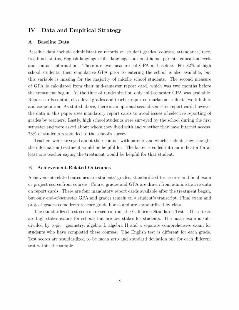
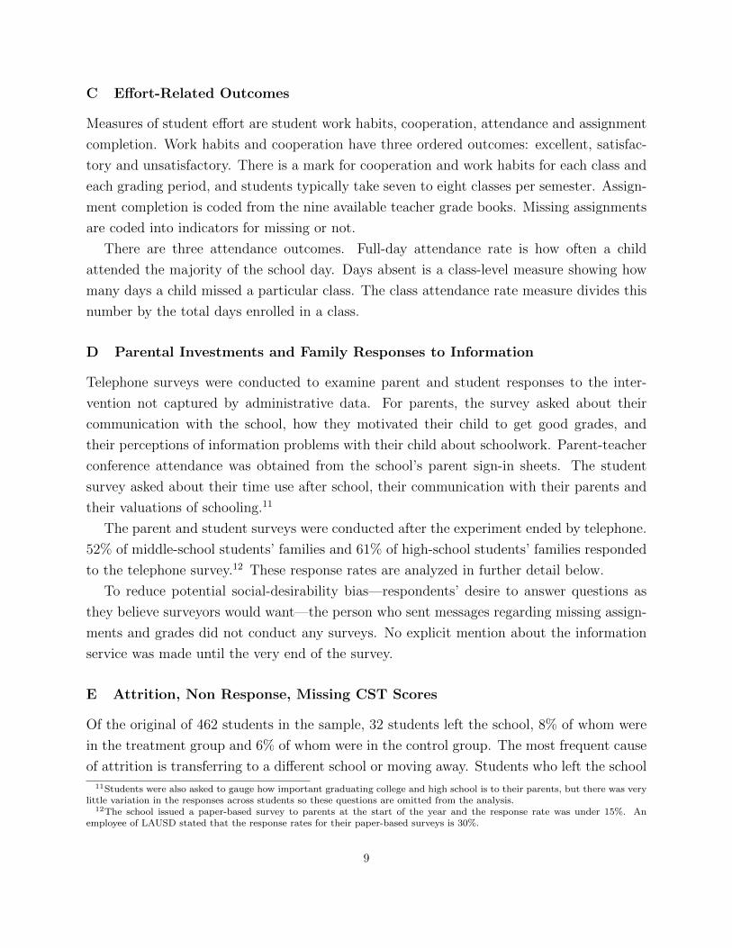
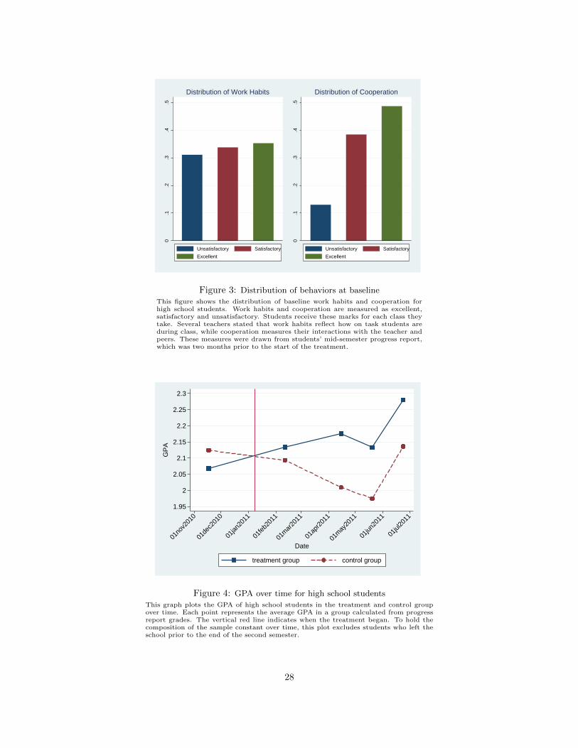
Figures 2 and 3 depict GPA and teacher-marked behavior distributions from the manda-

tory report card at baseline for all students.14 For every report card, work habits and

cooperation are graded as excellent, satisfactory or unsatisfactory for each student’s class.

Teachers describe the work habits grade as measuring how on task a student is while co-

operation reflects how respectful their classroom behavior is. Figure 3 shows the majority

of students receive satisfactory or excellent marks for class cooperation and only 10% of

students receive an unsatisfactory mark. Work-habit grades are more uniformly distributed

across the three possible marks.

13For comparison, LAUSD has said their non-response rate for parent surveys is roughly double this number.14For high school students, 22% of students have a baseline GPA of 1.00 or below, while 19% of students have 3.00 or above.

10

Table 1 presents baseline-summary statistics across the treatment group and the control

group for high school students. Panel A contains these statistics for the original sample

while Panel B excludes attriters to show the balance of the sample used for estimations.

Measures of works habits and cooperation are coded into indicators for unsatisfactory or not

and excellent or not. Of the 13 measures, one difference—the fraction of female students—is

significantly different (p-value of .078) between the treatment and control group in Panel A.

All results are robust to adding gender as a control. Work habits and students’ cumulative

GPA from their prior grades are better (but not significantly) for the control group than the

treatment group. Panel B shows that baseline GPA is .06 points higher for the control group

than the treatment group in the sample used for analysis, and as shown below, results are

sensitive to this control. One concern with this baseline difference is mean reversion, however

students’ prior GPA, which is a cumulative measure of their GPA over several years, also

shows the treatment group is lower achieving than the control group. In addition, GPA for

the control group is highly persistent from the end of the first semester to the end of the

second semester. A regression of the latter on the former yields a coefficient near one.15

G Empirical Strategy

The empirical analyses estimate intent-to-treat effects. Families in the treatment group may

have received fewer or no notifications because their child has special needs (13 families); the

guidance counselor requested them removed from the list due to family instability (two fam-

ilies); or the family speaks a language other than Spanish, English or Korean (two families).

All of these families are included in the treatment group.

To measure the effect of additional information on various outcomes, I estimate the fol-

lowing

yi = α + β ∗ Treatmenti +X ′iγ + εi (2)

Control variables in X include baseline GPA and cumulative GPA from each student’s prior

school, grade indicators and strata indicators. The results are robust to various specifications

so long as a baseline measure of GPA is controlled for, which most likely makes a difference

due to the .06 point difference at baseline.

I estimate equation 2 with GPA as a dependent variable. To discern whether there were

any differential effects by subject or for “targeted” classes—those classes for which a teacher

shared a grade book to participate in the information treatment—I also use class grades as

15Mean reversion does occur between students’ prior GPA and their baseline GPA, however this reversion does not differ bytreatment status (results available on request).

11

a dependent variable.16 This regression uses the same controls as 2 above but the standard

errors are clustered at the student level.17 End-of-semester grades are coded on a four-point

scale to match GPA calculations.18

Similar to class grades, there is a work habit mark and a cooperation mark for each

student’s class as well. I estimate the effect of additional information on these marks using

an ordered Probit model that pools together observations across grading periods and clusters

standard errors at the student level. The controls are the same as above with additional

grading-period fixed effects. I report marginal effects at the means, but the average of the

marginal effects yields similar results.

Effects on full-day attendance and attendance at the classroom level use the same speci-

fication and controls as the specifications for GPA and class grades, respectively.

V Results

The Effect of the Treatment on School-to-Parent Contact

Table 2 assesses the effect of the treatment on survey measures of school-to-parent contact.

Parents were asked how often the school contacted them during the last month of school

regarding their child’s grades or schoolwork. During this time all parents had been sent a

progress report about their child’s grades. The first column shows how much more often the

treatment group in high school was contacted by the school than the control group, control-

ling for baseline GPA and cumulative GPA from students’ prior schools.19 The treatment

increased contact from the school regarding their child’s grades and schoolwork by 187%

relative to the control group. The dependent variable in the second column measures the

fraction of people that were contacted by the school more than once. This fraction increases

by 158% relative to the control group. The treatment had large effects on both the extensive

margin of contact and the intensive margin of contact from the school regarding student

grades.

Recall that the experiment was contaminated when the middle school teachers had an

employee call their students regarding missing assignments. Mechanically, there should be

a positive effect for middle school families since parents did receive messages via the treat-

ment. The employee who contacted families regarding missing work did so for all students—

16Recall that only nine of the 14 teachers updated their grade books often enough so that assignment-related information couldbe provided to parents. The class-grades regression estimates whether those nine teachers’ classes showed greater achievementgains than the classes of teachers who did not update grades often enough to participate.

17Clustering at the teacher level or two-way clustering by teacher and student yield marginally smaller standard errors.18A is coded as 4, B as 3, C as 2, D as 1 and F as 0.19The results without controls are extremely similar.

12

treatment and control—likely resulting in parents being contacted more than once regarding

the same missing assignment. While there is no measure of how often parents were contacted

with new information, if the contamination were significant, we would expect school-contact

effects to be smaller for the middle school sample. The results are considerably weaker for

the middle school students. Contact increased by 106% and the fraction contacted increased

by 69%.

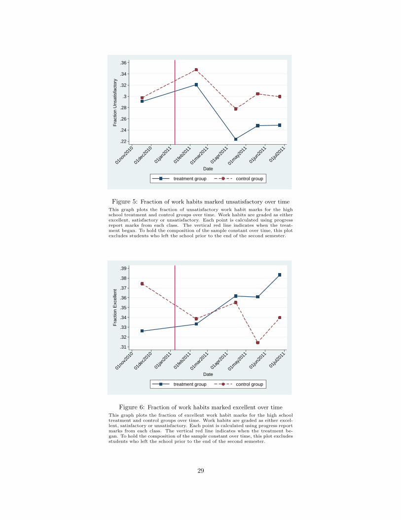
A Effects on GPA

Figure 4 tracks average GPA in the treatment and control groups over time. The red vertical

line indicates when the treatment began, which is about one month before the first semester

ended in mid February. There is a steady decrease in GPA for the control group after

the first semester ends in February followed by a spike upward during the final grading

period. The treatment group does not experience this decline and still improves in the final

grading period. Teachers reported that students work less in the beginning and middle of

the semester and “cram” during the last grading period to bring up their GPA, which may

negatively affect learning (Donovan, Figlio and Rush, 2006).

The regressions in Table 3 reinforce the conclusions drawn from the graphs described

above. Column (1) shows the effect on GPA with no controls. The increase is .15 and is

not significant, however the treatment group had a .06 point lower GPA at baseline. Adding

a control for baseline GPA raises the effect to .20 points and is significant at the 5% level

(column (2)). The standard errors decrease by 35%. The third column adds controls for

GPA from students’ prior schools and grade level indicators. The treatment effect increases

slightly to .23 points. The latter converts to a .19 standard deviation increase in GPA over

the control group. The results in Table 4 show that grades for classes Table 4 shows estimates

of the treatment effect on class grades. Column (1) shows this effect is nearly identical to

the effect on final GPA.20 Column (2) shows the effect on targeted classes—those classes for

which a teacher was asked to participate and that teacher provided a grade book so that

messages could be sent home regarding missing work. This analysis is underpowered, but

the interaction term is positive and not significant (p-value equals .16). Columns (3) and

(4) show that math classes had greater gains than English classes (p-values equal .11 and

.85, respectively). This effect disparity coincides with the difference in effects shown later

for standardized tests scores.

The last column shows the effects for students in which at least one teacher thought

additional information would be especially helpful for them. The treatment effect is negative20The similarity in effects between this unweighted regression and the regression on GPA is because there is small variation

in the number of classes students take.

13

but not significant (p-value equals .24). Most likely there was no differential effect for these

students, and if anything the effect appears negative. Teachers appear to have no additional

information about whom the treatment would be most helpful for. While teachers generally

take in new students every year, the teachers in this sample had known students for three

months at the time this variable was measured at baseline.

Even though grading standards are school specific, the impact on GPA is important.

In the short run, course grades in required classes determine high school graduation and

higher education eligibility. In the longer run, several studies find that high school GPA is

the best predictor of college performance and attainment (for instance Geiser and Santelices,

2007). GPA is also significantly correlated with earnings even after controlling for test scores

(Rosenbaum, 1998; French et al., 2010). 21

B Effects on Final Exams and Projects and Standardized Test scores

Additional information causes exam and final project scores to improve by .16 standard

deviations (significant at the 5% level, Table 5). However, teachers enter missing finals as

zeros into the grade book. On average, 18% percent of final exams and projects were not

submitted by the control group. The effect on the fraction of students turning in their final

exam or project is large and significant. Additional information reduces this fraction missing

by 42%, or 7.5 percentage points.

Ideally, state-mandated tests are administered to all students, which would help separate

out the treatment effect on participation from the effect on their score. Unfortunately,

many students did not take these tests, and as shown above, missing a score is correlated

with treatment status and treatment-control imbalance—prior test scores of treatment-group

students are .26 lower and baseline GPA .13 points lower (results not shown). To see whether

those who did not take the test responded to the treatment differently than those who did

take the test, I compare the GPA results of those who took the standardized tests with those

who did not. Specifically, the indicator for treatment is interacted with an indicator for

having a math test score or English test score as follows.

GPAi = β0 + β1 ∗ Treatmenti + β2 ∗ Treatmenti ∗ 1(HasScorei) +X ′iγ + εi

Where the variable HasScorei is an indicator for either having an English test score or

having a math test score. The coefficient on the interaction term, β2, indicates whether

21One caveat, however, is that the mechanisms that generate these correlations may differ from the mechanisms underlyingthe impact of additional information on GPA.

14

those who have a test score experienced different effects on GPA than those who do not have

a test score. This achievement effect might correlate with the achievement effect on test

scores. If β2 is large, it suggests how the test-score results might be biased—upwards if β2

is positive and downwards is β2 is negative.

Table A.4 shows the results of this analysis. The coefficients on the interaction term for

having a score is insignificant (p-value equals .14) but is large and negative. Thus there is

some evidence that the treatment effect is smaller for those with test scores compared to

those without, which may bias the estimates on test scores downward.

To account for this potential bias, the effects on math and English test scores are shown

with a varying number of controls. The first and fourth columns in Table 6 control only for

baseline GPA. The effect on math and English scores are .08 and -.04 standard deviations

respectively. Columns (2) and (5) add controls for prior test scores, demographic charac-

teristics and test subject. The treatment effect on math scores is .21 standard deviations,

but remains near zero for English scores. Finally, if the treatment induces lower performing

students to take the test, then those with higher baseline GPA might be less affected by this

selection. This means we might see a positive coefficient on the interaction term between

baseline GPA and the treatment. Columns (3) and (6) add this interaction term. While the

interaction term is small for English scores, for math scores it implies that someone with the

average GPA of 2.01 has a .20 standard deviations higher math score due to the additional

information provided to their parents.22

This disparity between math and English gains is not uncommon. Bettinger (2010) finds

financial incentives increase math scores but not English scores and discusses several previous

studies (Reardon, Cheadle, and Robinson, 2008; Rouse, 1998) on educational interventions

that exhibit this difference as well. There are three apparent reasons the information inter-

vention may have had a stronger effect on math than English. First, the math teachers in

this sample provided more frequent information on assignments that allowed more messages

to be sent to parents. Potentially, this frequency might mean students fall less behind.23

Second, 30% of students are classified as “limited-English proficient,” which means they are

English-language learners and need to pass a proficiency test three years in a row to be

reclassified. Looking at class grades, these students tend to actually perform better in En-

glish classes, though interacting the treatment with indicators for language proficiency and

English classes yields a large and negative coefficient (results not shown). In contrast, this

coefficient is negative but 75% smaller when the interaction term includes an indicator for

22This marginal effect at the mean is significant at the 5% level.23This theory is difficult to test since there is no within-class variation in grade-book upkeep or message frequency conditional

on missing an assignment.

15

math classes rather than English classes. This means that the treatment effect for students

with limited English skills is associated with smaller gains for English than math, which

may in part drive the disparity in effects. Lastly, math assignments might provide better

preparation for the standardized tests compared to English assignments if they more closely

approximate the problems on the test.

C Effects on Behaviors and Assignment Completion

The effects on work habits and cooperation are consistent with the effects on GPA. Figure 5

shows that the treatment group exhibits less unsatisfactory work habits than control group,

on average. Figure 6 shows that excellent work habits increase steadily for the treatment

group over time. Excellent cooperation, shown in Figure 8, dips in the middle of the semester

but rises at the end. The average levels of uncooperative behavior exhibit a similar pattern

to unsatisfactory work habits (Figures 7).

Table 7 provides the ordered-Probit estimates for work habits and cooperation (Panel

A). Additional information reduces the probability of unsatisfactory work habits by 24%,

or a six-percentage point reduction from the overall probability at the mean. This result

mirrors the effect on excellent work habits for high school students, which increases by seven-

percentage points at the mean. The probability of unsatisfactory cooperation is reduced by

25% and the probability of excellent cooperation improves by 13%.

Panel B shows OLS estimates of the effects on attendance. The effect on full-day atten-

dance is positive though not significant, however full-day attendance rates are already above

90% and students are more likely to skip a class than a full day. Analysis at the class level

shows positive and significant effects. The treatment reduces classes missed by 28%. The

final column of Panel B contains the estimated probability of missing an assignment. At

the mean, 20% of assignments are not turned in. Assignments include all work, classwork

and homework, and the grade books do not provide enough detail to discern one from the

other.24 At the mean, the treatment decreases the probability of missing an assignment by

25%.

The behavior effects indicate that one mechanism the additional information operates

through is increased productivity during school hours. Assignments may be started in class

but might have to be completed at home if they are not finished during class (e.g. a lab

report for biology or chemistry, or worksheets and writing assignments in history and English

classes). If students do not complete this work in class due to poor attendance or a slow work

pace, they may not do it at home. The information treatment discourages low attendance

24Several teachers said that classwork is much more likely to be completed than work assigned to be done at home.

16

and in-class productivity, which in turn may increase assignment completion.

D Mechanisms

The goal of this is section is to understand how parents used the additional information pro-

vided by the treatment, how students responded outside of school, and how the information

affected parents.

How Parents Used the Additional Information

Panel A of Table 8 shows how parents used the information. Parents were asked how many

privileges they took away from their child in the last month of school, which increased by

nearly 100% for the treatment group (column (1)). The most common privilege revoked by

parents involved electronic devices—cell phones, television, Internet use and video games—

followed by seeing friends.25 Parents also spoke about college more often to their child,

perhaps emphasizing the future returns to schooling in addition to the threat of punishment.

Interestingly, parents in the treatment group asked about homework less during the last

month of school, though the coefficient is not significant. The negative sign could be due to

parents’ interpretation of the question in that they exclude messages from the school from

their count. Or, parents might substitute away from asking about this from their children

if they realize the information provided via the treatment is more reliable. Lastly, children

were asked how often they received help with their homework from their parents on a three

point scale (“never,” “sometimes,” or “always,” coded from zero to two). The final column

of Panel A shows the coefficient is positive but not significant. Overall, more information

appears to facilitate parents ability to incentivize their children to do well in school.

How Students Responded

The first three columns of Panel B show how students’ work habits changed outside of

school. Tutoring attendance over the semester increased 42%. The coefficient is marginally

insignificant at standard levels (p-value equals .11). Tutoring was offered by teachers after

school for free. The positive effect on tutoring is at least partially due to several teachers’

requirement that missing work be made up during their after school tutoring to prevent

cheating. The second column shows the effect on whether students did their homework at

the last minute, which was coded from zero to two for “never,” “sometimes” or “always.”

25An open-ended question also asked students how their parents respond when they receive good grades. 41% said theirparents take them out or buy them something, 50% said their parents are happy, proud or congratulate them, and 9% saidtheir parents do not do anything.

17

Students in the treatment group were significantly less likely to do their homework at the

last minute. Nonetheless, student study hours at home did not significantly increase, which

implies that most of the gains in achievement are due to improved work habits at school.

The remaining two columns of Panel B show students’ valuations of schooling on a four-point

scale. Students in the treatment group are more likely to say grades are important, but no

more likely to say that college is important. One interpretation of these results is that grades

are important because students will be punished if they do not do well, but their intrinsic

valuation of schooling has not changed.

Information Problems and Information Demand

Panel C shows that some parents lacked awareness of the information problems with their

child regarding school work. Column (1) reports the answers to the question, “Does your

child not tell you enough about his or her school work or grades?” Parents in the treatment

group are almost twice as likely to say yes as parents in the control group. This answer

may reflect parents’ about their understanding of the A–F grading system. 11% of parents

responded that they did not understand it or were unsure of the meaning of the scale. 40%

of parents did not graduate high school and many are not from the United States. Other

countries use different grading scales, which might contribute to parents’ unfamiliarity and

their reliance on their children for information.26

Coinciding with the awareness of information problems, the second and third columns

show that parents increased their demand for information regarding their child’s school-

work and progress. Over the last semester, parents in the treatment group were much more

likely to contact the school regarding the latter (85% more), and this is corroborated by the

school’s data on parent-teacher conference attendance, which increased by 53%. The guid-

ance counselor reported that parents arranged meetings with her because of the additional

information. This increased contact could partly be due to the limited nature of the addi-

tional information in the messages home and the conflict it created in the household. The

information came directly from the grade book and no further details could be provided. If a

child denied missing an assignment, provided an excuse or parents otherwise needed further

information, parents might have wanted to speak directly to the counselor or teacher. The

treatment appears to make parents aware of communication problems between themselves

and their children, which in turns spurs demand for information from the school.

Finally, the last column reports answers to whether parents agree they can help their

child do their best at school. Parents in the treatment group are 16 percentage points more

26This knowledge deficit is salient enough to LAUSD that they have begun to offer free classes to parents to teach them aboutthe school system, graduation requirements, what to ask during conferences and other school-related information.

18

likely to say yes.

Confounding Mechanisms and Spillovers

One concern with the student level, within-classroom randomization is that additional in-

formation may have had no effect on student effort, and in turn learning, because teachers

artificially raised treatment-group student grades to reduce any hassle from parental contact.

A second concern is that teachers paid more attention to treatment-group students at the

expense of attention for control-group students, biasing effects away from zero. While these

are potential issues, several results undermine support for these interpretations.

The most definitive results contradicting these interpretations are the significant effects on

measures of student effort and parental investments that are less likely to be manipulated by

teachers. The treatment group has higher attendance rates, higher levels of student-reported

effort such as tutoring attendance and timely work completion, and a greater fraction of

completed assignments. These results suggest that students indeed exerted more effort as a

result of the information treatment. Consistent with this interpretation, the survey evidence

from parents suggests that treatment-group parents took steps to motivate their children in

response to the additional information beyond those of control-group parents, such as more

intensive use of incentives.

It is also plausible that teachers who did not participate in the information intervention

were less aware of who is in the treatment group versus the control group and therefore less

likely to change their behavior as a result of the experiment. Consistent with the results

above, the class-level analysis shows that students’ grades also improved in the classes of

these non-participating teachers (see Table 4, column two).

Third, an analysis of treatment effects on control group students provides some evidence

on whether the control group’s grades increased or decreased as a result of the treatment.

Though the experiment was not designed to examine peer effects, random assignment at the

student level generates classroom-level variation in the fraction of students treated. Table A.5

shows the results from a regression of control students’ class grades on the fraction of students

treated in each respective class. While not statistically significant (p-value equals .27), the

point estimate implies that a 25 percentage point increase in the fraction of students treated

in a given classroom causes control group students’ grades to increase by .14 points (.09

standard deviations). This provides some evidence that improved behaviors of treatment-

group students may have had positive spillovers onto control-group students’ achievement

such that the overall effects are likely biased toward zero.

19

VI Middle School Results

Table 9 summarizes the effects on achievement and effort-related outcomes for middle school

students, which are mostly small and not significantly different from zero. These results

are consistent with the effects on how parents used the additional information, how children

responded, and parents’ awareness and demand for information (Table 10). Based on these

results and the contamination, it is difficult to discern what effect the treatment would have

had on younger students.

There are several reasons the additional information may have had less effect on younger

children. First, the middle school students have less margin to improve: Their GPA is

almost a full standard deviation higher than high school students’ GPA, middle school stu-

dents miss 7.5% of their assignments compared to high school students who miss 20% of

their assignments, and attendance and behavior are also better for middle school students.

However if this were the only cause for small effects, there could still be an impact on stu-

dents who were lower-performing at baseline. Unfortunately the study is underpowered to

examine subgroups in the middle school, however if anything students with higher GPA re-

spond more positively to additional information (results not shown). A second reason there

might be smaller effects for middle school students is that parents might be able to control

younger children better than older children. It might be less costly for parents to motivate

their children or information problems arise less frequently. There is some support for this

hypothesis since teacher-measured behavior at baseline is better for middle school students

than high school students, which might correlate with parents’ ability to control their child.

Third, the repeated messages to middle school parents through the information treatment

and the contamination by the school employee may have annoyed them. If they had already

resolved an issue such as a missing assignment, receiving a second message regarding that

work might have been confusing and frustrating. Parents could have viewed the informa-

tion treatment as less reliable given the lack of coordination about school-to-parent contact

and started ignoring it, which might explain the small negative coefficients on several middle

school outcomes. Lastly, parents of middle-school students might already obtain information

about their child’s education more actively, which is reflected in the higher parent-teacher

conference attendance. In addition, a comparison of the control groups in the high school

and middle school shows that parents of middle school students are more likely to take away

privileges from their children, be aware of information problems, contact the school about

their child’s grades, and feel that they can help their child try their best than parents of

high school students in the control group.27 It is possible that the contamination caused

27Results available upon request.

20

this higher level of involvement—meaning messages home did affect middle school parents—

or it could be that these parents were already more involved than high school parents. If

the latter, it leaves open the question of why this involvement wanes as children get older;

perhaps parents perceive they have less control of their child’s effort or that they no longer

know how to help them. In short, the effect of additional information on younger children

is inconclusive.

VII Conclusion and Cost effectiveness

This paper uses an experiment to answer how information asymmetries between parents and

their children affect human capital investment and achievement. The results show these

problems can be significant and their effect on achievement large. Additional information

to parents about their child’s missing assignments and grades helps parents motivate their

children more effectively, but also changes parents’ beliefs about the quality of information

they receive from their child. Parents become more aware that their child does not tell them

enough about their academic progress. These mechanisms drive an almost .20 standard

deviation improvement in math standardized test scores and GPA for high school students.

There is no estimated effect on middle-school family outcomes, however there was severe

contamination in the middle school sample. One positive aspect of this contamination is

that it reflects teachers’ perceptions of the intervention. In response to this experiment,

the school and a grade-book company collaborated to develop a feature that automatically

text messages parents about their child’s missing assignments directly from teachers’ grade

books.

Importantly, this paper demonstrates a potentially cost-effective way to bolster student

achievement: Provide parents frequent and detailed grade-book information. Contacting

parents via text message, phone call or email took approximately three minutes per student.

Gathering and maintaining contact numbers adds five minutes of time per child, on average.

The time to generate a missing-work report can be almost instantaneous or take several

minutes depending on the grade book used and the coordination across teachers.28 For

this experiment it was roughly five minutes. Teacher overtime pay varies across districts

and teacher characteristics, but a reasonable estimate prices their time at $40 per hour. If

teachers were paid to coordinate and provide information, the total cost per child per .10

standard-deviation increase in GPA or math scores would be $156. Automating aspects of

this process through a grade book could reduce this costs further. Relative to other effective

28Some grade book programs can produce a missing assignment report for all of a student’s classes.

21

interventions targeting adolescent achievement, this cost is quite low.

However it is important to consider how well these results extrapolate to other contexts.

While the student population is fairly representative of a large, urban school district like

Los Angeles Unified, there are several parameters of the education-production function that

determine the effectiveness of increasing information to parents. The framework in Section

II illustrates this point. Two salient factors are teacher and parent characteristics. Teacher

quality affects both the capability of the school to provide information and the impact of

student effort on achievement. If teachers do not frequently grade assignments, it is difficult

to increase the amount of information to parents. Nine of the fourteen teachers in the sample

maintained their grade books often enough to effectively participate in the experiment. It is

not known whether this is a typical amount or not. In this experiment, the positive effects

spilled over to classes for which there was little grade book information. Also, teachers

at this school generally accepted work after the requested due date. Parents were notified

about missing assignments that they could still help their child complete. This scheme

might allow parents to overcome a child’s high discount rate by immediately monitoring

and incentivizing the work they must make up. The results may be weaker if parents are

only notified about work prior to the due date or about work students can no longer turn

in. Even if information can be provided, and this engenders greater effort from students,

the effects on achievement depend on the quality of the work teachers supply. Students may

work harder but show no gains in measures of learning. For parents, the effects may differ by

demographic characteristics as well. Information changes parental beliefs, and this effect may

apply less to parents who know the school system well and have greater resources to invest

in their children. Finally, the treatment lasted six months. The negative information about

academic performance could create tension at home that might impact outcomes differently

over the long run. 29

Overall, the results support a model of human capital investment that incorporates infor-

mation asymmetries between parents and their children. This experiment suggests providing

information lowered monitoring costs for parents, which increased incentives and improved

student effort and achievement. More broadly, parental monitoring is positively linked to

number of behavioral outcomes, such as crime and health behaviors (Kerr and Stattin, 2000).

Future research could examine how parent-child information frictions affect other parental

investments in their children as well.

29The cost-effectiveness analysis excludes this potential cost to parents and children.

22

References

[1] Aaronson, Daniel, Lisa Barrow and William Sander (2007). “Teachers and Student

Achievement in the Chicago Public High Schools,” Journal of Labor Economics, vol

25(1), 95-135.

[2] Abdulkadiroglu, Atila, Joshua D. Angrist, Susan M. Dynarski, Thomas J. Kane and

Parag A. Pathak (2011). “Accountability and Flexibility in Public Schools: Evidence

from Boston’s Charters and Pilots,” The Quarterly Journal of Economics, 126, 699-748.

[3] Andrabi, Tahir, Jishnu Das and Asim Ijaz Khwaja (2009). “Report Cards: The Impact

of Providing School and Child Test-Scores on Educational Markets,” Mimeo, Harvard

University.

[4] Angrist, Joshua D., Susan M. Dynarski, Thomas J. Kane, Parag A. Pathak, Christopher

R. Walters (2010). “Inputs and Impacts in Charter Schools: KIPP Lynn,” American

Economic Review: Papers and Proceedings, vol 100(2), 239-243.

[5] Angrist, Joshua D. and Victor Lavy (2002). “The Effects of High Stakes High School

Achievement Awards: Evidence from a Randomized Trial,” American Economic Review,

vol 99(4), 1384-1414.

[6] Avvisati, Francesco, Marc Gurgand, Nina Guyon and Eric Maurin (2010). “The Influence

of Parents and Peers on Pupils: A Randomized Experiment,” Mimeo, Paris School of

Economics.

[7] Berry, James (2011). “Child Control in Education Decisions: An Evaluation of Targeted

Incentives to Learn in India,” Mimeo, Cornell University.

[8] Bettinger, Eric P. (2010). “Paying to Learn: The Effect of Financial Incentives on Ele-

mentary School Test Scores,” NBER Working Paper No. 16333.

[9] Bettinger, Eric, Bridget T. Long, Philip Oreopoulos and Lisa Sanbonmatsu (2009). “The

Role of Simplification and Information in College Decisions: Results from the H&R Block

FAFSA Experiment,” NBER Working Paper No. 15361.

[10] Bettinger, Eric and Robert Slonim (2007). “Patience in Children: Evidence from Ex-

perimental Economics,” Journal of Public Economics, vol 91(1-2): 343-363.

[11] Bridgeland, John M., John J. Dilulio, Ryan T. Streeter, and James R. Mason (2008).

One Dream, Two Realities: Perspectives of Parents on America’s High Schools, Civic

Enterprises and Peter D. Hart Research Associates.

23

[12] Buddin, Richard (2010). “How Effective Are Los Angeles Elemen-

tary Teachers and Schools?” Retrieved online on April 2011, from

http://s3.documentcloud.org/documents/19505/how-effective-are-los-angeles-

elementary-teachers-and-schools.pdf.

[13] Bursztyn, Leonardo and Lucas Coffman (2011). “The Schooling Decision: Family Pref-

erences, Intergenerational Conflict, and Moral Hazard in the Brazilian Favelas,” Mimeo,

UCLA Anderson.

[14] Cameron, Colin, Jonah Gelbach and Douglas Miller (2008). “Bootstrap-Based Improve-

ments for Inference with Clustered Standard Errors,” The Review of Economics and

Statistics, vol 90(3): 414-427.

[15] Cunha, F., James J. Heckman, Lance Lochner and Dimitriy V. Masterov (2006), “Chap-

ter 12 Interpreting the Evidence on Life Cycle Skill Formation,” Handbook of the Eco-

nomics of Education, vol 1: 697-812.

[16] Dobbie, Will and Roland G. Fryer (2011). “Are High Quality Schools Enough to Close

the Achievement Gap? Evidence from the Harlem Children’s Zone,” American Journal:

Applied Economics, vol 3(3), 158-187.

[17] French, Michael, Jenny Homer and Philip K. Robins (2010). “What You Do in High

School Matters: The Effects of High School GPA on Educational Attainment and Labor

Market Earnings in Adulthood.” Mimeo, University of Miami, Department of Economics.

[18] Fryer, Roland G. (2010). “Financial Incentives and Student Achievement: Evidence

from Randomized Trials,” NBER Working Paper No. 15898.

[19] Fryer, Roland G. (2011). “Teacher Incentives and Student Achievement: Evidence from

New York City Public Schools,” NBER Working Paper No. 16850.

[20] Gelser, Saul and Marla V. Santelices (2007). “Validity of High-School Grades in Predict-

ing Student Success Beyond the Freshman Year: High-School Record vs. Standardized

Tests as Indicators of Four-Year College Outcomes,” Research & Occasional Paper Series:

CSHE.6.07.

[21] Hastings, Justine S. and Jeffrey M. Weinstein (2008). “Information, School Choice, and

Academic Achievement: Evidence from two Experiments” Quarterly Journal of Eco-

nomics, vol 123(4) 1373-1414.

[22] Houtenville, Andrew J. and Karen Smith Conway (2008), “Parental Effort, School Re-

sources and Student Achievement,” Journal of Human Resources, vol 43(2): 437-453.

24

[23] Jacob, Brian and Lars Lefgren (2008). “Can Principals identify Effective Teachers? Evi-

dence on Subjective Performance Evaluation in Education,” Journal of Labor Economics,

vol 26(1), 101-136.

[24] Kerr, Margaret and Hakan Stattin (2000). “Parental Monitoring: A Reinterpretation,”

Child Development, vol 71(4), 1072-1085.

[25] Levitt, Steven D., John A. List, Susanne Neckermann and Sally Sadoff (2011). “The

Impact of Short-Term Incentives on Student Perofrmance” Mimeo, University of Chicago,

Becker Friedman Institute.

[26] Los Angeles Unified School District (2009). “Memorandum of Un-

derstanding Between Los Angeles Unified School District and United

Teachers Los Angeles.” Retrieved on January 10, 2011, from

http://publicschoolchoice.lausd.net/sites/default/files/Los%20Angeles%20Pilot%

20Schools%20Agreement%20%28Signed%29.pdf.

[27] Los Angeles Unified School District (2011). School Report Cards. Retrieved on January

10, 2011, from http://getreportcard.lausd.net/reportcards/reports.jsp.

[28] Miller, Cynthia, James Riccio and Jared Smith (2009). “A Preliminary Look at Early

Educational Results of the Opportunity NYC-Family Rewards Program” MDRC.

[29] Rivkin, Steven G., Eric A. Hanushek and John F. Kain (2005). “Teachers, Schools, and

Academic Achievement,” Econometrica, vol 73(2), 417-458.

[30] Rockoff, Jonah E., Douglas O. Staiger, Thomas J. Kane and Eric S. Taylor (2010).

“Information and Employee Evaluation: Evidence from a Randomized Intervention in

Public Schools,” NBER Working Paper No. 16240.

[31] Rosenbaum, James E. (1998). “College-for-All: Do Students Understand What College

Demands?” Social Pyschology of Education, vol 2(1) 55-80.

[32] SFGate.com (2010). Poll Finds Most Blame Parents for School Woes. Retrieved on

January 10, 2011, from http://articles.sfgate.com/2010-12-12/news/25188015 1 parents-

united-responsible-education-student-discipline.

[33] Springer, Matthew G., D. Ballou, L. Hamilton, V. Le, J.R. Lockwood, D. McCaffrey,

M. Pepper and B. Stecher (2010). “Teacher Pay for Performance: Experimental Evi-

dence from the Project on Incentives in Teacher,” Nashville, TN: National Center on

Performance Incentives at Vanderbilt University.

25

[34] Steinberg, Laurence, Lia O’Brien, Elizabeth Cauffman, Sandra Graham, Jennifer

Woolard and Marie Banich (2009). “Age Differences in Future Orientation and Delay

Discounting” Child Development, vol 80(1): 28-44.

[35] Time Magazine (2010). TIME Poll Results: Americans’ Views on Teacher Tenure,

Merit Pay and Other Education Reforms. Retrieved online on January 10, 2011, from

http://www.time.com/time/nation/article/0,8599,2016994,00.html#ixzz1dFb1oSwE.

[36] Todd, Petra and Kenneth I. Wolpin (2007), “The Production of Cognitive Achievement

in Children: Home, School and Racial Test Score Gaps,” Journal of Human Capital, vol

1(1): 91-136.

[37] Weinberg, Bruce (2001), “An Incentive Model of the Effect of Parental Income on Chil-

dren,” Journal of Political Economy, vol 109(2): 266-280.

26

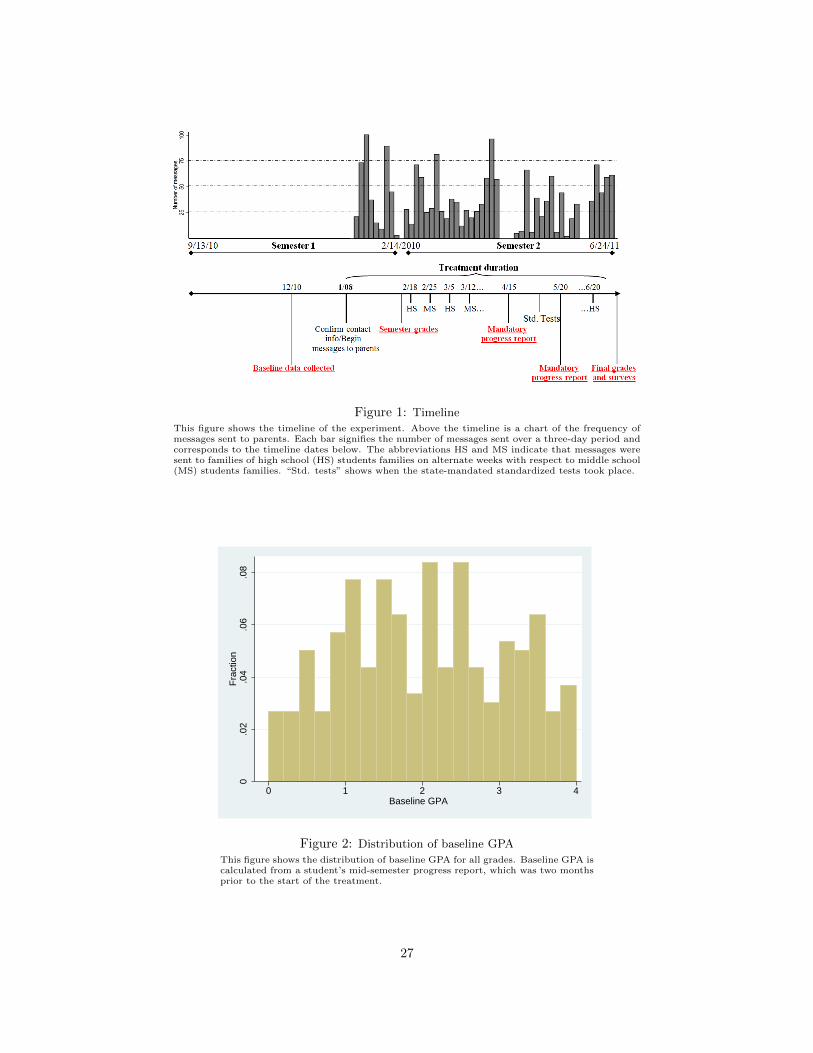
Figure 1: Timeline

This figure shows the timeline of the experiment. Above the timeline is a chart of the frequency ofmessages sent to parents. Each bar signifies the number of messages sent over a three-day period andcorresponds to the timeline dates below. The abbreviations HS and MS indicate that messages weresent to families of high school (HS) students families on alternate weeks with respect to middle school(MS) students families. “Std. tests” shows when the state-mandated standardized tests took place.

0.0

2.0

4.0

6.0

8F

ract

ion

0 1 2 3 4Baseline GPA

Figure 2: Distribution of baseline GPA

This figure shows the distribution of baseline GPA for all grades. Baseline GPA iscalculated from a student’s mid-semester progress report, which was two monthsprior to the start of the treatment.

27

0.1

.2.3

.4.5

Distribution of Work Habits

Unsatisfactory Satisfactory

Excellent

0.1

.2.3

.4.5

Distribution of Cooperation

Unsatisfactory Satisfactory

Excellent

Figure 3: Distribution of behaviors at baseline

This figure shows the distribution of baseline work habits and cooperation forhigh school students. Work habits and cooperation are measured as excellent,satisfactory and unsatisfactory. Students receive these marks for each class theytake. Several teachers stated that work habits reflect how on task students areduring class, while cooperation measures their interactions with the teacher andpeers. These measures were drawn from students’ mid-semester progress report,which was two months prior to the start of the treatment.

1.95

2

2.05

2.1

2.15

2.2

2.25

2.3

GP

A

01no

v201

0

01de

c201

0

01jan

2011

01fe

b201

1

01m

ar20

11

01ap

r201

1

01m

ay20

11

01jun

2011

01jul

2011

Date

treatment group control group

Figure 4: GPA over time for high school students

This graph plots the GPA of high school students in the treatment and control groupover time. Each point represents the average GPA in a group calculated from progressreport grades. The vertical red line indicates when the treatment began. To hold thecomposition of the sample constant over time, this plot excludes students who left theschool prior to the end of the second semester.

28

.22

.24

.26

.28

.3

.32

.34

.36

Fra

ctio

n U

nsat

isfa

ctor

y

01no

v201

0

01de

c201

0

01jan

2011

01fe

b201

1

01m

ar20

11

01ap

r201

1

01m

ay20

11

01jun

2011

01jul

2011

Date

treatment group control group

Figure 5: Fraction of work habits marked unsatisfactory over time

This graph plots the fraction of unsatisfactory work habit marks for the highschool treatment and control groups over time. Work habits are graded as eitherexcellent, satisfactory or unsatisfactory. Each point is calculated using progressreport marks from each class. The vertical red line indicates when the treat-ment began. To hold the composition of the sample constant over time, this plotexcludes students who left the school prior to the end of the second semester.

.31

.32

.33

.34

.35

.36

.37

.38

.39

Fra

ctio

n E

xcel

lent

01no

v201

0

01de

c201

0

01jan

2011

01fe

b201

1

01m

ar20

11

01ap

r201

1

01m

ay20

11

01jun

2011

01jul

2011

Date

treatment group control group

Figure 6: Fraction of work habits marked excellent over time

This graph plots the fraction of excellent work habit marks for the high schooltreatment and control groups over time. Work habits are graded as either excel-lent, satisfactory or unsatisfactory. Each point is calculated using progress reportmarks from each class. The vertical red line indicates when the treatment be-gan. To hold the composition of the sample constant over time, this plot excludesstudents who left the school prior to the end of the second semester.

29

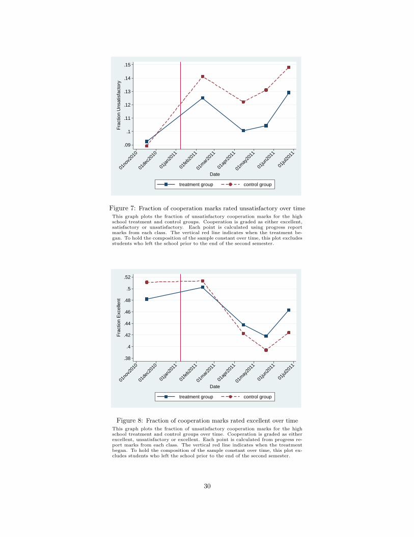
.09

.1

.11

.12

.13

.14

.15

Fra

ctio

n U

nsat

isfa

ctor

y

01no

v201

0

01de

c201

0

01jan

2011

01fe

b201

1

01m

ar20

11

01ap

r201

1

01m

ay20

11

01jun

2011

01jul

2011

Date

treatment group control group

Figure 7: Fraction of cooperation marks rated unsatisfactory over time

This graph plots the fraction of unsatisfactory cooperation marks for the highschool treatment and control groups. Cooperation is graded as either excellent,satisfactory or unsatisfactory. Each point is calculated using progress reportmarks from each class. The vertical red line indicates when the treatment be-gan. To hold the composition of the sample constant over time, this plot excludesstudents who left the school prior to the end of the second semester.

.38

.4

.42

.44

.46

.48

.5

.52

Fra

ctio

n E

xcel

lent

01no

v201

0

01de

c201

0

01jan

2011

01fe

b201

1

01m

ar20

11

01ap

r201

1

01m

ay20

11

01jun

2011

01jul

2011

Date

treatment group control group

Figure 8: Fraction of cooperation marks rated excellent over time

This graph plots the fraction of unsatisfactory cooperation marks for the highschool treatment and control groups over time. Cooperation is graded as eitherexcellent, unsatisfactory or excellent. Each point is calculated from progress re-port marks from each class. The vertical red line indicates when the treatmentbegan. To hold the composition of the sample constant over time, this plot ex-cludes students who left the school prior to the end of the second semester.

30

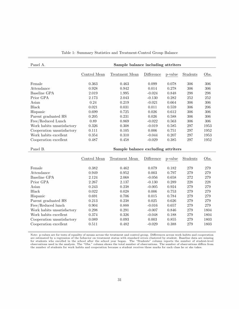
Table 1: Summary Statistics and Treatment-Control Group Balance

Panel A. Sample balance including attriters

Control Mean Treatment Mean Difference p-value Students Obs.

Female 0.363 0.463 0.099 0.078 306 306Attendance 0.928 0.942 0.014 0.278 306 306Baseline GPA 2.019 1.995 -0.024 0.848 298 298Prior GPA 2.173 2.043 -0.130 0.282 252 252Asian 0.24 0.219 -0.021 0.664 306 306Black 0.021 0.031 0.011 0.559 306 206Hispanic 0.699 0.725 0.026 0.612 306 306Parent graduated HS 0.205 0.231 0.026 0.588 306 306Free/Reduced Lunch 0.89 0.869 -0.022 0.563 306 306Work habits unsatisfactory 0.326 0.308 -0.019 0.585 297 1953Cooperation unsatisfactory 0.111 0.105 0.006 0.751 297 1952Work habits excellent 0.354 0.310 -0.044 0.207 297 1953Cooperation excellent 0.487 0.458 -0.029 0.385 297 1952

Panel B. Sample balance excluding attriters

Control Mean Treatment Mean Difference p-value Students Obs.

Female 0.382 0.462 0.079 0.182 279 279Attendance 0.949 0.952 0.003 0.797 279 279Baseline GPA 2.124 2.068 -0.056 0.658 272 279Prior GPA 2.267 2.137 -0.130 0.289 228 228Asian 0.243 0.238 -0.005 0.924 279 279Black 0.022 0.028 0.006 0.753 279 279Hispanic 0.691 0.706 0.015 0.784 279 279Parent graduated HS 0.213 0.238 0.025 0.626 279 279Free/Reduced lunch 0.904 0.888 -0.016 0.657 279 279Work habits unsatisfactory 0.298 0.291 -0.007 0.846 279 1804Work habits excellent 0.374 0.326 -0.048 0.188 279 1804Cooperation unsatisfactory 0.089 0.093 0.003 0.855 279 1803Cooperation excellent 0.511 0.482 -0.029 0.388 279 1803

Note: p-values are for tests of equality of means across the treatment and control group. Differences across work habits and cooperationare estimated by a regression of the behavior on treatment status with standard errors clustered by student. Baseline data are missingfor students who enrolled in the school after the school year began. The “Students” column reports the number of student-levelobservations used in the analysis. The “Obs.” column shows the total number of observations. The number of observations differs fromthe number of students for work habits and cooperation because a student receives these marks for each class he or she takes.

31

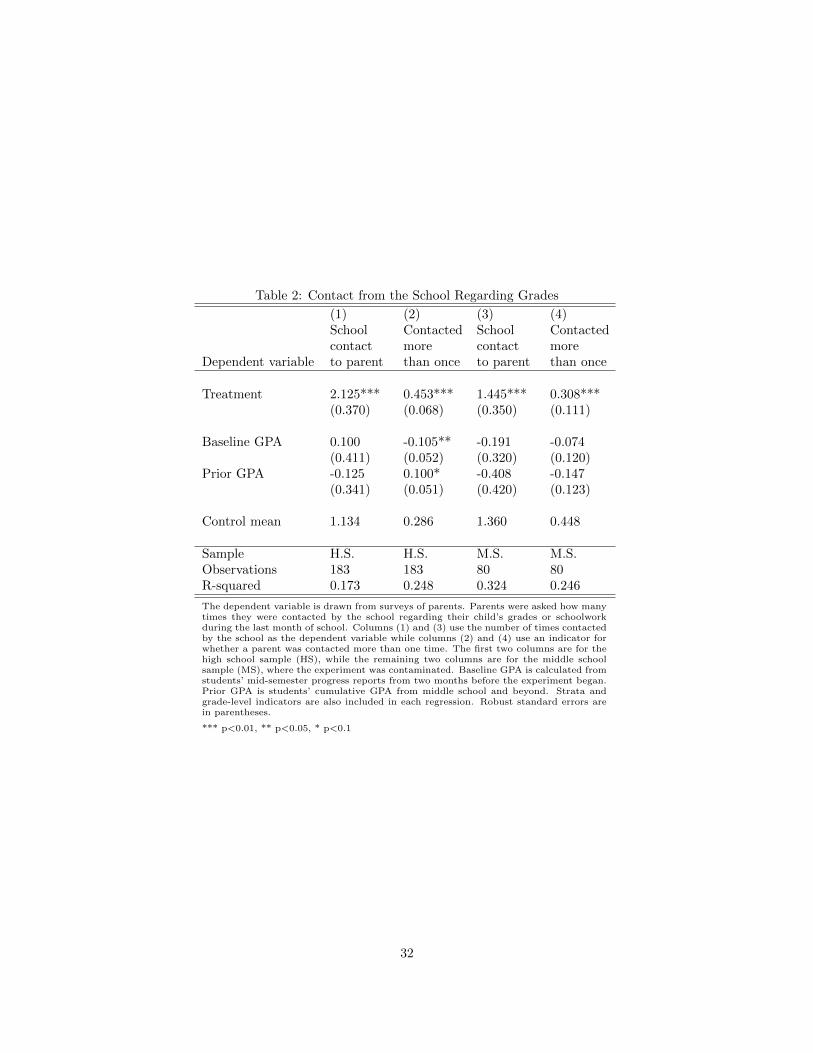
Table 2: Contact from the School Regarding Grades

(1) (2) (3) (4)

Dependent variable

Schoolcontactto parent

Contactedmorethan once

Schoolcontactto parent

Contactedmorethan once

Treatment 2.125*** 0.453*** 1.445*** 0.308***(0.370) (0.068) (0.350) (0.111)

Baseline GPA 0.100 -0.105** -0.191 -0.074(0.411) (0.052) (0.320) (0.120)

Prior GPA -0.125 0.100* -0.408 -0.147(0.341) (0.051) (0.420) (0.123)

Control mean 1.134 0.286 1.360 0.448

Sample H.S. H.S. M.S. M.S.Observations 183 183 80 80R-squared 0.173 0.248 0.324 0.246

The dependent variable is drawn from surveys of parents. Parents were asked how manytimes they were contacted by the school regarding their child’s grades or schoolworkduring the last month of school. Columns (1) and (3) use the number of times contactedby the school as the dependent variable while columns (2) and (4) use an indicator forwhether a parent was contacted more than one time. The first two columns are for thehigh school sample (HS), while the remaining two columns are for the middle schoolsample (MS), where the experiment was contaminated. Baseline GPA is calculated fromstudents’ mid-semester progress reports from two months before the experiment began.Prior GPA is students’ cumulative GPA from middle school and beyond. Strata andgrade-level indicators are also included in each regression. Robust standard errors arein parentheses.

*** p<0.01, ** p<0.05, * p<0.1

32

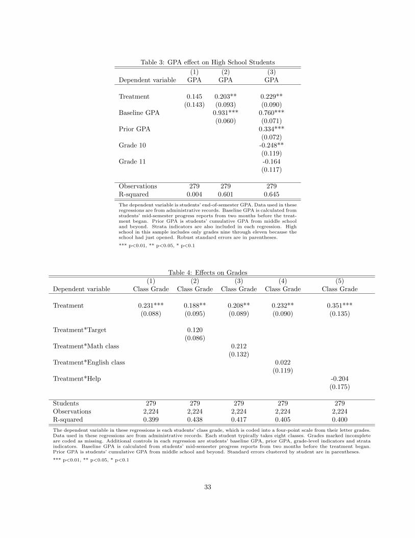
Table 3: GPA effect on High School Students

(1) (2) (3)Dependent variable GPA GPA GPA

Treatment 0.145 0.203** 0.229**(0.143) (0.093) (0.090)

Baseline GPA 0.931*** 0.760***(0.060) (0.071)

Prior GPA 0.334***(0.072)

Grade 10 -0.248**(0.119)

Grade 11 -0.164(0.117)

Observations 279 279 279R-squared 0.004 0.601 0.645

The dependent variable is students’ end-of-semester GPA. Data used in theseregressions are from administrative records. Baseline GPA is calculated fromstudents’ mid-semester progress reports from two months before the treat-ment began. Prior GPA is students’ cumulative GPA from middle schooland beyond. Strata indicators are also included in each regression. Highschool in this sample includes only grades nine through eleven because theschool had just opened. Robust standard errors are in parentheses.

*** p<0.01, ** p<0.05, * p<0.1

Table 4: Effects on Grades(1) (2) (3) (4) (5)

Dependent variable Class Grade Class Grade Class Grade Class Grade Class Grade

Treatment 0.231*** 0.188** 0.208** 0.232** 0.351***(0.088) (0.095) (0.089) (0.090) (0.135)

Treatment*Target 0.120(0.086)

Treatment*Math class 0.212(0.132)

Treatment*English class 0.022(0.119)

Treatment*Help -0.204(0.175)

Students 279 279 279 279 279Observations 2,224 2,224 2,224 2,224 2,224R-squared 0.399 0.438 0.417 0.405 0.400

The dependent variable in these regressions is each students’ class grade, which is coded into a four-point scale from their letter grades.Data used in these regressions are from administrative records. Each student typically takes eight classes. Grades marked incompleteare coded as missing. Additional controls in each regression are students’ baseline GPA, prior GPA, grade-level indicators and strataindicators. Baseline GPA is calculated from students’ mid-semester progress reports from two months before the treatment began.Prior GPA is students’ cumulative GPA from middle school and beyond. Standard errors clustered by student are in parentheses.

*** p<0.01, ** p<0.05, * p<0.1

33

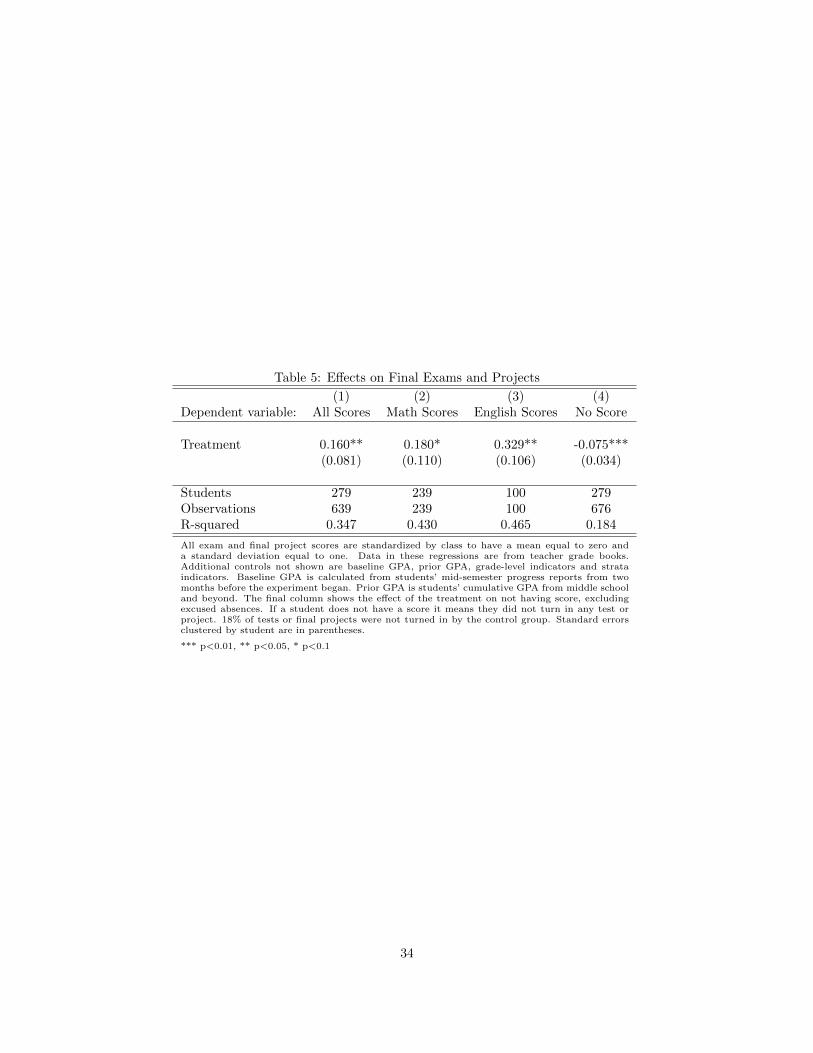
Table 5: Effects on Final Exams and Projects

(1) (2) (3) (4)Dependent variable: All Scores Math Scores English Scores No Score

Treatment 0.160** 0.180* 0.329** -0.075***(0.081) (0.110) (0.106) (0.034)

Students 279 239 100 279Observations 639 239 100 676R-squared 0.347 0.430 0.465 0.184

All exam and final project scores are standardized by class to have a mean equal to zero anda standard deviation equal to one. Data in these regressions are from teacher grade books.Additional controls not shown are baseline GPA, prior GPA, grade-level indicators and strataindicators. Baseline GPA is calculated from students’ mid-semester progress reports from twomonths before the experiment began. Prior GPA is students’ cumulative GPA from middle schooland beyond. The final column shows the effect of the treatment on not having score, excludingexcused absences. If a student does not have a score it means they did not turn in any test orproject. 18% of tests or final projects were not turned in by the control group. Standard errorsclustered by student are in parentheses.

*** p<0.01, ** p<0.05, * p<0.1

34

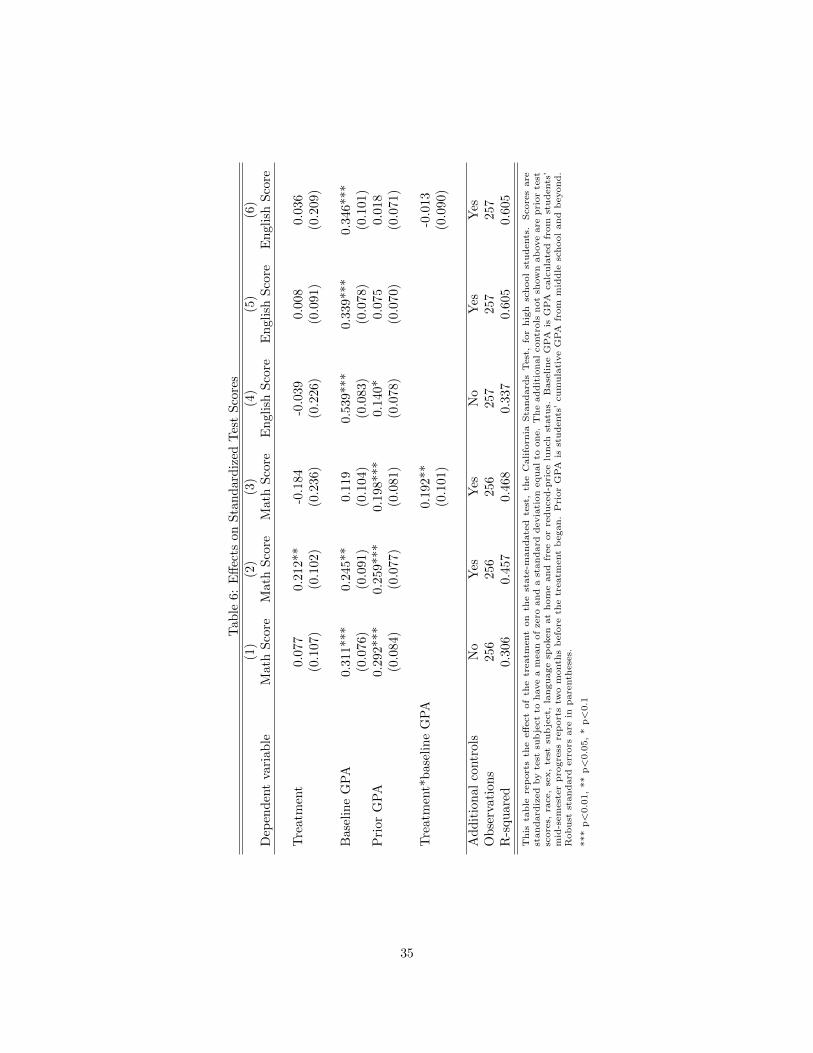
Tab

le6:

Eff

ects

on

Sta

nd

ard

ized

Tes

tS

core

s(1

)(2

)(3

)(4

)(5

)(6

)D

epen

den

tva

riab

leM

ath

Sco

reM

ath

Sco

reM

ath

Sco

reE

ngli

shS

core

En

gli

shS

core

En

gli

shS

core

Tre

atm

ent

0.07

70.2

12**

-0.1

84

-0.0

39

0.0

08

0.0

36

(0.1

07)

(0.1

02)

(0.2

36)

(0.2

26)

(0.0

91)

(0.2

09)

Bas

elin

eG

PA

0.31

1***

0.2

45**

0.1

19

0.5

39***

0.3

39***

0.3

46***

(0.0

76)

(0.0

91)

(0.1

04)

(0.0

83)

(0.0

78)

(0.1

01)

Pri

orG

PA

0.29

2***

0.2

59***

0.1

98***

0.1

40*

0.0

75

0.0

18

(0.0

84)

(0.0

77)

(0.0

81)

(0.0

78)

(0.0

70)

(0.0

71)

Tre

atm

ent*

bas

elin

eG

PA

0.1

92**

-0.0

13

(0.1

01)

(0.0

90)

Ad

dit

ion

alco

ntr

ols

No

Yes

Yes

No

Yes

Yes

Ob

serv

atio

ns

256

256

256

257

257

257

R-s

qu

ared

0.30

60.4

57

0.4

68

0.3

37

0.6

05

0.6

05

This

table

rep

ort

sth

eeff

ect

of

the

treatm

ent

on

the

state

-mandate

dte

st,

the

Califo

rnia

Sta

ndard

sT

est

,fo

rhig

hsc

hool

students

.Score

sare

standard

ized

by

test

sub

ject

tohave

am

ean

of

zero

and

ast

andard

devia

tion

equal

toone.

The

addit

ional

contr

ols

not

show

nab

ove

are

pri

or

test

score

s,ra

ce,

sex,

test

sub

ject,

language

spoken

at

hom

eand

free

or

reduced-p

rice

lunch

statu

s.B

ase

line

GP

Ais

GP

Acalc

ula

ted

from

students

’m

id-s

em

est

er

pro

gre

ssre

port

stw

om

onth

sb

efo

reth

etr

eatm

ent

began.

Pri

or

GP

Ais

students

’cum

ula

tive

GP

Afr

om

mid

dle

school

and

beyond.

Robust

standard

err

ors

are

inpare

nth

ese

s.

***

p<

0.0

1,

**

p<

0.0

5,

*p<

0.1

35

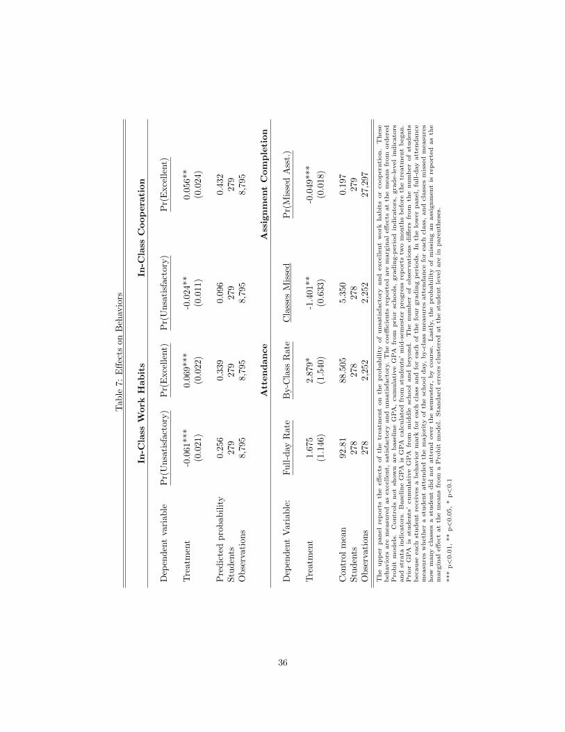
Tab

le7:

Eff

ects

on

Beh

avio

rs

In-C

lass

Work

Habits

In-C

lass

Coopera

tion

Dep

end

ent

vari

able

Pr(

Un

sati

sfact

ory

)P

r(E

xce

llen

t)P

r(U

nsa

tisf

act

ory

)P

r(E

xce

llen

t)

Tre

atm

ent

-0.0

61***

0.0

69***

-0.0

24**

0.0

56**

(0.0

21)

(0.0

22)

(0.0

11)

(0.0

24)

Pre

dic

ted

pro

bab

ilit

y0.

256

0.3

39

0.0

96

0.4

32

Stu

den

ts27

9279

279

279

Ob

serv

atio

ns

8,795

8,7

95

8,7

95

8,7

95

Attendance

AssignmentCompletion

Dep

end

ent

Var

iab

le:

Fu

ll-d

ayR

ate

By-C

lass

Rate

Cla

sses

Mis

sed

Pr(

Mis

sed

Ass

t.)

Tre

atm

ent

1.67

52.8

79*

-1.4

01**

-0.0

49***

(1.1

46)

(1.5

40)

(0.6

33)

(0.0

18)

Con

trol

mea

n92

.81

88.5

05

5.3

50

0.1

97

Stu

den

ts27

8278

278

279

Ob

serv

atio

ns

278

2,2

52

2,2

52

27,2

97

The

upp

er

panel

rep

ort

sth

eeff

ects

of

the

treatm

ent

on

the

pro

babilit

yof

unsa

tisf

acto

ryand

excellent

work

habit

sor

coop

era

tion.

These

behavio

rsare

measu

red

as

excellent,

sati

sfacto

ryand

unsa

tisf

acto

ry.

The

coeffi

cie

nts

rep

ort

ed

are

marg

inal

eff

ects

at

the

means

from

ord

ere

dP

robit

models

.C

ontr

ols

not

show

nare

base

line

GP

A,

cum

ula

tive

GP

Afr

om

pri

or

schools

,gra

din

g-p

eri

od

indic

ato

rs,

gra

de-l

evel

indic

ato

rsand

stra

tain

dic

ato

rs.

Base

line

GP

Ais

GP

Acalc

ula

ted

from

students

’m

id-s

em

est

er

pro

gre

ssre

port

stw

om

onth

sb

efo

reth

etr

eatm

ent

began.

Pri

or

GP

Ais

students

’cum

ula

tive

GP

Afr

om

mid

dle

school

and

beyond.

The

num

ber

of

obse

rvati

ons

diff

ers

from

the

num

ber

of

students

because

each

student

receiv

es

ab

ehavio

rm

ark

for

each

cla

ssand

for

each

of

the

four

gra

din

gp

eri

ods.

Inth

elo

wer

panel,

full-d

ay

att

endance

measu

res

wheth

er

ast

udent

att

ended

the

majo

rity

of

the

school

day,

by-c

lass

measu

res

att

endance

for

each

cla

ss,

and

cla

sses

mis

sed

measu

res

how

many

cla

sses

ast

udent

did

not

att

end

over

the

sem

est

er,

by

cours

e.

Last

ly,

the

pro

babilit

yof

mis

sing

an

ass

ignm

ent

isre

port

ed

as

the

marg

inal

eff

ect

at

the

means

from

aP

robit

model.

Sta

ndard

err

ors

clu

stere

dat

the

student

level

are

inpare

nth

ese

s.

***

p<

0.0

1,

**

p<

0.0

5,

*p<

0.1

36

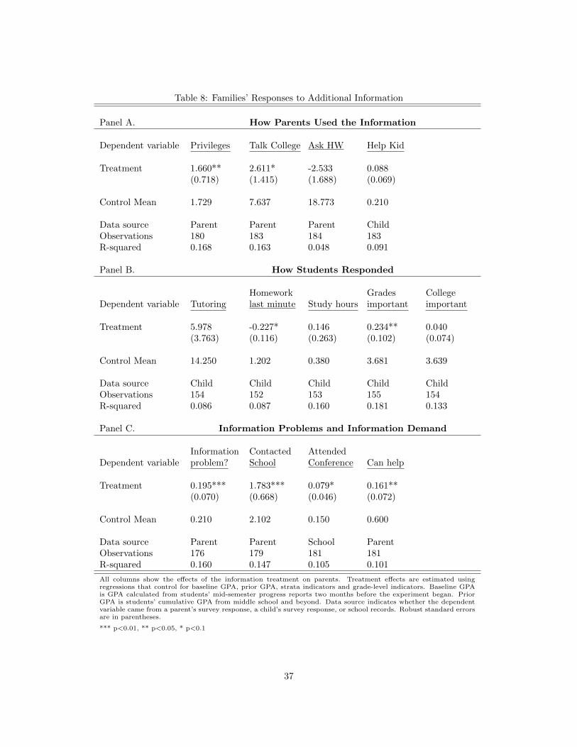
Table 8: Families’ Responses to Additional Information

Panel A. How Parents Used the Information

Dependent variable Privileges Talk College Ask HW Help Kid

Treatment 1.660** 2.611* -2.533 0.088(0.718) (1.415) (1.688) (0.069)

Control Mean 1.729 7.637 18.773 0.210

Data source Parent Parent Parent ChildObservations 180 183 184 183R-squared 0.168 0.163 0.048 0.091

Panel B. How Students Responded

Dependent variable TutoringHomeworklast minute Study hours

Gradesimportant

Collegeimportant

Treatment 5.978 -0.227* 0.146 0.234** 0.040(3.763) (0.116) (0.263) (0.102) (0.074)

Control Mean 14.250 1.202 0.380 3.681 3.639

Data source Child Child Child Child ChildObservations 154 152 153 155 154R-squared 0.086 0.087 0.160 0.181 0.133

Panel C. Information Problems and Information Demand

Dependent variableInformationproblem?

ContactedSchool

AttendedConference Can help

Treatment 0.195*** 1.783*** 0.079* 0.161**(0.070) (0.668) (0.046) (0.072)

Control Mean 0.210 2.102 0.150 0.600

Data source Parent Parent School ParentObservations 176 179 181 181R-squared 0.160 0.147 0.105 0.101

All columns show the effects of the information treatment on parents. Treatment effects are estimated usingregressions that control for baseline GPA, prior GPA, strata indicators and grade-level indicators. Baseline GPAis GPA calculated from students’ mid-semester progress reports two months before the experiment began. PriorGPA is students’ cumulative GPA from middle school and beyond. Data source indicates whether the dependentvariable came from a parent’s survey response, a child’s survey response, or school records. Robust standard errorsare in parentheses.

*** p<0.01, ** p<0.05, * p<0.1

37

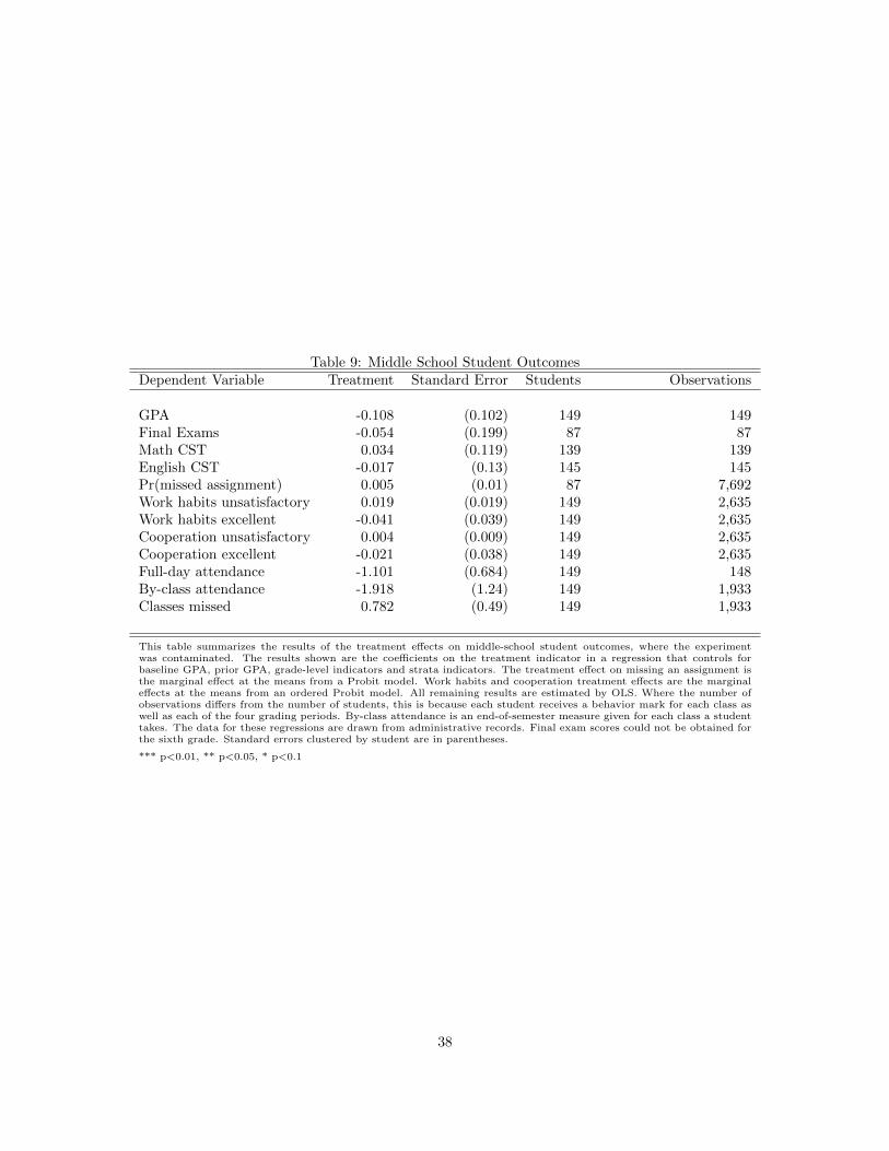
Table 9: Middle School Student OutcomesDependent Variable Treatment Standard Error Students Observations

GPA -0.108 (0.102) 149 149Final Exams -0.054 (0.199) 87 87Math CST 0.034 (0.119) 139 139English CST -0.017 (0.13) 145 145Pr(missed assignment) 0.005 (0.01) 87 7,692Work habits unsatisfactory 0.019 (0.019) 149 2,635Work habits excellent -0.041 (0.039) 149 2,635Cooperation unsatisfactory 0.004 (0.009) 149 2,635Cooperation excellent -0.021 (0.038) 149 2,635Full-day attendance -1.101 (0.684) 149 148By-class attendance -1.918 (1.24) 149 1,933Classes missed 0.782 (0.49) 149 1,933

This table summarizes the results of the treatment effects on middle-school student outcomes, where the experimentwas contaminated. The results shown are the coefficients on the treatment indicator in a regression that controls forbaseline GPA, prior GPA, grade-level indicators and strata indicators. The treatment effect on missing an assignment isthe marginal effect at the means from a Probit model. Work habits and cooperation treatment effects are the marginaleffects at the means from an ordered Probit model. All remaining results are estimated by OLS. Where the number ofobservations differs from the number of students, this is because each student receives a behavior mark for each class aswell as each of the four grading periods. By-class attendance is an end-of-semester measure given for each class a studenttakes. The data for these regressions are drawn from administrative records. Final exam scores could not be obtained forthe sixth grade. Standard errors clustered by student are in parentheses.

*** p<0.01, ** p<0.05, * p<0.1

38

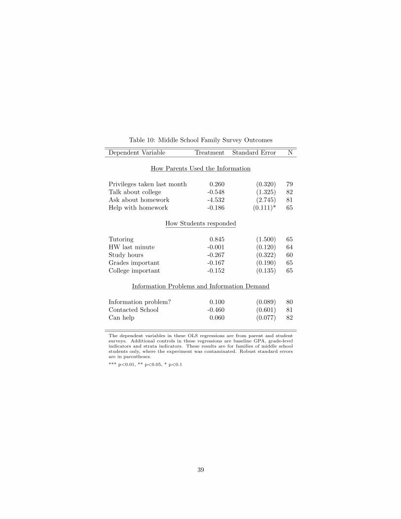
Table 10: Middle School Family Survey Outcomes

Dependent Variable Treatment Standard Error N

How Parents Used the Information

Privileges taken last month 0.260 (0.320) 79Talk about college -0.548 (1.325) 82Ask about homework -4.532 (2.745) 81Help with homework -0.186 (0.111)* 65

How Students responded

Tutoring 0.845 (1.500) 65HW last minute -0.001 (0.120) 64Study hours -0.267 (0.322) 60Grades important -0.167 (0.190) 65College important -0.152 (0.135) 65

Information Problems and Information Demand

Information problem? 0.100 (0.089) 80Contacted School -0.460 (0.601) 81Can help 0.060 (0.077) 82

The dependent variables in these OLS regressions are from parent and studentsurveys. Additional controls in these regressions are baseline GPA, grade-levelindicators and strata indicators. These results are for families of middle schoolstudents only, where the experiment was contaminated. Robust standard errorsare in parentheses.

*** p<0.01, ** p<0.05, * p<0.1

39

Appendix for Online Publication

Table A.1: Attrition(1) (2) (3) (4) (5) (6)

Dependent variable Left the Sample

Treatment -0.016 -0.012 0.008 0.026 0.020 0.025(0.029) (0.026) (0.018) (0.031) (0.031) (0.027)

7th grade 0.005 -0.032(0.025) (0.026)

8th grade 0.061 -0.017(0.046) (0.027)

Baseline GPA -0.058 -0.001(0.037) (0.022)

Prior GPA 0.007 -0.047*(0.036) (0.027)

Full-day attendance 0.496 -0.838***(0.306) (0.255)

Female -0.012 -0.003(0.022) (0.029)

Black 0.937*** 0.160(0.115) (0.121)

Hispanic -0.160 0.067(0.133) (0.044)

Asian -0.107 0.099**(0.132) (0.045)

Free/Reduced Lunch 0.027 -0.026(0.018) (0.040)

10th grade 0.089** 0.042(0.041) (0.034)

11th grade 0.039 0.036(0.036) (0.038)

Control mean 0.041 0.068

Sample MS MS MS H.S. H.S. H.S.Observations 156 156 156 306 306 306R-squared 0.031 0.050 0.500 0.037 0.050 0.243

The dependent variable in these regressions is an indicator for having left the school. Columns (1)-(3) show thecorrelates of leaving for the middle school (MS). Baseline GPA is from mid-semester report cards two months beforethe treatment began and prior GPA is students’ cumulative GPA from previous grades. Columns (4)-(6) show thesecorrelates for the high school (HS) sample only. Robust standard errors are in parentheses.

*** p<0.01, ** p<0.05, * p<0.1

40

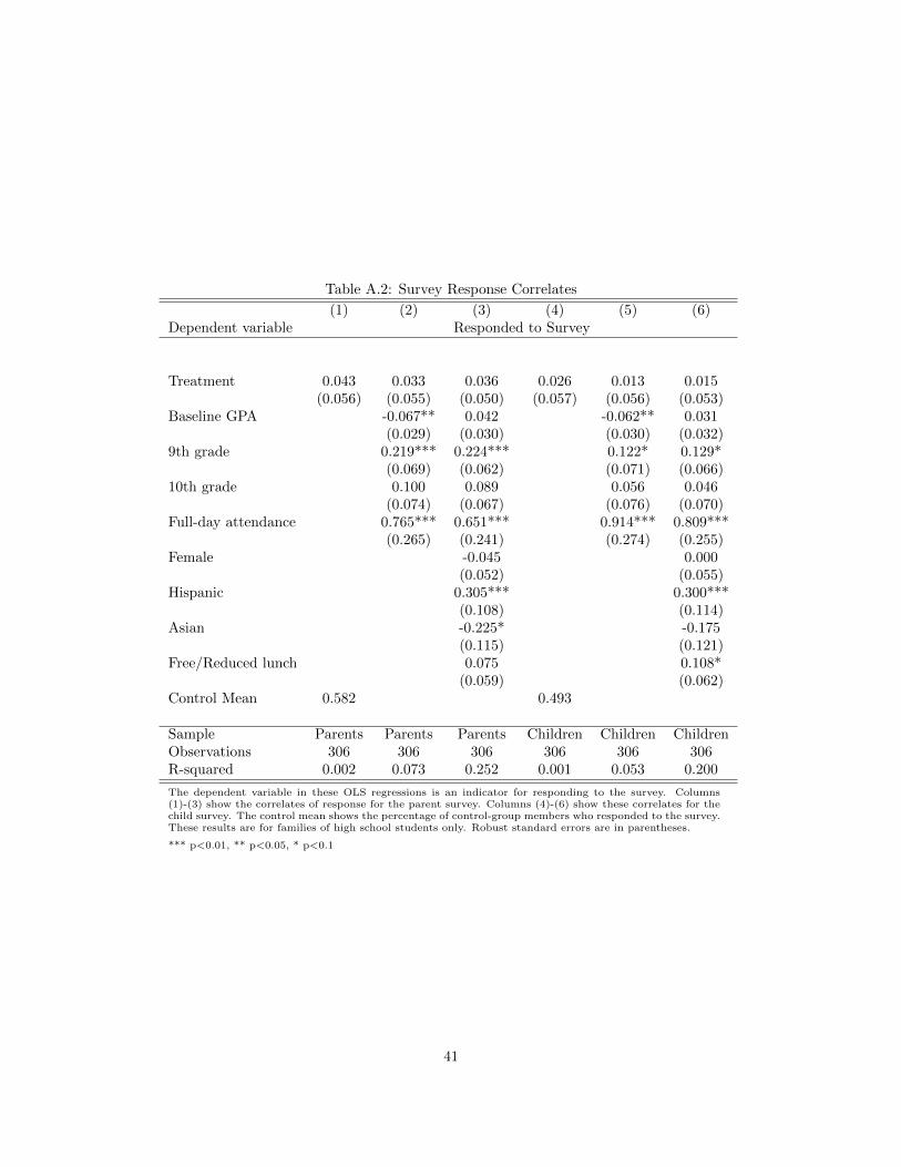
Table A.2: Survey Response Correlates

(1) (2) (3) (4) (5) (6)Dependent variable Responded to Survey

Treatment 0.043 0.033 0.036 0.026 0.013 0.015(0.056) (0.055) (0.050) (0.057) (0.056) (0.053)

Baseline GPA -0.067** 0.042 -0.062** 0.031(0.029) (0.030) (0.030) (0.032)

9th grade 0.219*** 0.224*** 0.122* 0.129*(0.069) (0.062) (0.071) (0.066)

10th grade 0.100 0.089 0.056 0.046(0.074) (0.067) (0.076) (0.070)

Full-day attendance 0.765*** 0.651*** 0.914*** 0.809***(0.265) (0.241) (0.274) (0.255)

Female -0.045 0.000(0.052) (0.055)

Hispanic 0.305*** 0.300***(0.108) (0.114)

Asian -0.225* -0.175(0.115) (0.121)

Free/Reduced lunch 0.075 0.108*(0.059) (0.062)

Control Mean 0.582 0.493

Sample Parents Parents Parents Children Children ChildrenObservations 306 306 306 306 306 306R-squared 0.002 0.073 0.252 0.001 0.053 0.200

The dependent variable in these OLS regressions is an indicator for responding to the survey. Columns(1)-(3) show the correlates of response for the parent survey. Columns (4)-(6) show these correlates for thechild survey. The control mean shows the percentage of control-group members who responded to the survey.These results are for families of high school students only. Robust standard errors are in parentheses.

*** p<0.01, ** p<0.05, * p<0.1

41

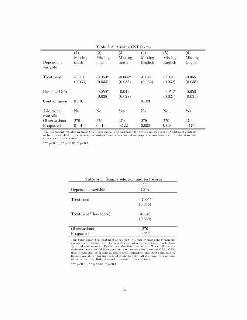
Table A.3: Missing CST Scores

(1) (2) (3) (4) (5) (6)

Dependentvariable

Missingmath

Missingmath

Missingmath

MissingEnglish

MissingEnglish

MissingEnglish

Treatment -0.054 -0.060* -0.065* -0.047 -0.051 -0.056(0.033) (0.033) (0.035) (0.032) (0.032) (0.035)

Baseline GPA -0.050* -0.041 -0.053* -0.050(0.028) (0.028) (0.021) (0.031)

Control mean 0.110 0.103

Additionalcontrols

No No Yes No No Yes

Observations 279 279 279 279 279 279R-squared 0 .010 0.010 0.122 0.008 0.090 0.173

The dependent variable in these OLS regressions is an indicator for having no test score. Additional controlsinclude prior GPA, prior scores, test-subject indicators and demographic characteristics. Robust standarderrors are in parentheses.

*** p<0.01, ** p<0.05, * p<0.1

Table A.4: Sample selection and test scores

(1)Dependent variable GPA

Treatment 0.700**(0.356)

Treatment*(has score) -0.546(0.369)

Observations 279R-squared 0.653

This table shows the treatment effect on GPA, and interacts the treatmentvariable with an indicator for whether or not a student has a math stan-dardized test score an English standardized test score. These effects areestimated with an OLS regression that controls for baseline GPA, GPAfrom a students prior school, grade-level indicators and strata indicators.Results are shown for high school students only. All data are from admin-istrative records. Robust standard errors in parentheses.

*** p<0.01, ** p<0.05, * p<0.1

42

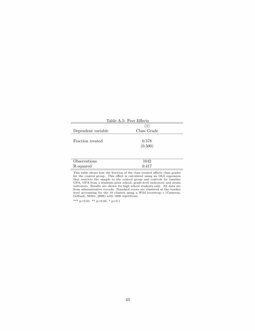
Table A.5: Peer Effects(1)

Dependent variable Class Grade

Fraction treated 0.578(0.500)

Observations 1042R-squared 0.417

This table shows how the fraction of the class treated affects class gradesfor the control group. This effect is calculated using an OLS regressionthat restricts the sample to the control group and controls for baselineGPA, GPA from a students prior school, grade-level indicators and strataindicators. Results are shown for high school students only. All data arefrom administrative records. Standard errors are clustered at the teacherlevel accounting for the 19 clusters using a Wild bootstrap t (Cameron,Gelbach, Miller, 2008) with 1000 repetitions.

*** p<0.01, ** p<0.05, * p<0.1

43