Price of Long-Run Temperature Shifts in Capital Markets

Ravi Bansal, Dana Kiku and Marcelo Ochoa∗

November 18, 2016

Abstract

We use the forward-looking information from the US and global capital markets to estimate

the economic impact of global warming, specifically, long-run temperature shifts. We find that

global warming carries a positive risk premium that increases with the level of temperature

and that has almost doubled over the last 80 years. Consistent with our model, virtually all

US equity portfolios have negative exposure (beta) to long-run temperature fluctuations. The

elasticity of equity prices to temperature risks across global markets is significantly negative

and has been increasing in magnitude over time along with the rise in temperature. We use

our empirical evidence to calibrate a long-run risks model with temperature-induced disasters in

distant output growth to quantify the social cost of carbon emissions. The model simultaneously

matches the projected temperature path, the observed consumption growth dynamics, discount

rates provided by the risk-free rate and equity market returns, and the estimated temperature

elasticity of equity prices. We find that the long-run impact of temperature on growth implies a

significant social cost of carbon emissions.

∗Ravi Bansal is affiliated with the Fuqua School of Business at Duke University and NBER, Dana Kiku is at theUniversity of Illinois at Urbana-Champaign, and Marcelo Ochoa is at the Federal Reserve Board. The analysis andconclusions set forth are those of the authors and do not indicate concurrence by other members of the research staffor the Board of Governors. We would like to thank Lars Hansen, Geoffrey Heal, Christian Traeger, Ricardo Colacito,Tony Smith, Thomas Maurer, Juhani Linnainmaa, Holger Kraft, and seminar participants at Duke University, theHong Kong University of Science and Technology, the University of Hong Kong, and the 2016 SED meeting for theirhelpful comments. The usual disclaimer applies.

Introduction

Global warming and its impact on the macro-economy is a matter of considerable importance (see

Stern (2007) and Nordhaus (2008)). However, measuring the economic costs of global warming

pose significant empirical challenges. This article shows that forward-looking equity prices that are

determined by the discounted value of future growth rates provide important information about the

cost of long-horizon temperature fluctuations. Using data from the US and global equity markets, we

document that persistent temperature shifts have a significant negative effect on aggregate wealth

and carry a positive risk premium in equity markets. We find that the risk premium for low-

frequency (i.e, long-run) temperature fluctuations has been increasing over time along with the rise

in temperature. To interpret our empirical evidence and to quantify the social cost of carbon, we

provide a temperature-augmented long-run risk model. Our model, calibrated to match financial

market data and our empirical evidence, implies that the social cost of carbon is quite large.

Our temperature-augmented long-run risks (LRR-T) model builds on the long-run risks

framework of Bansal and Yaron (2004) and accounts for the interaction between climate change,

economic growth and risk. To account for the potentially severe consequences of global warming,

the model features temperature-induced natural disasters in future output and growth.1 Disasters

are triggered when temperature breaches a threshold level (tipping point) and capture the idea of

tail risk related to global warming as discussed in Pindyck (2012). Different from the standard

integrated assessment (IAM) models, in which climate change is assumed to cause a deterministic

loss in output, in the LRR-T model, temperature is a source of economic risk — a persistent increase

in temperature rises the likelihood of breaching the temperature tipping point and causing economic

disasters. Temperature risks in our model affect aggregate wealth and asset valuations through the

variation in expected growth rates and discount rates. In particular, a rise in temperature raises

the marginal utility and lowers the current wealth to consumption ratio. Thus, temperature risks

carry a positive premium, which is reflected in prices of forward-looking assets such as equities. The

LRR-T model makes several predictions that guide our empirical work. First, consistent with the

consensus view, in the model, the most significant effects of global warming unfold in the relatively

1Earlier work on economic disasters includes Rietz (1988), Barro (2009), Gourio (2012), and Bansal, Kiku, andYaron (2010), among others.

1

distant future and, therefore, they are difficult to assess from the current and historical output

data. However, temperature risks have a measurable impact on current equity valuations. We

exploit this implication in our empirical work and use capital market data to estimate the price of

temperature risks. Second, the model predicts that the price of low-frequency temperature risks

and their risk premia increase with temperature. We test this implication using a conditional factor

model specification that allows for variation in the market price of long-run temperature risks.

Using a cross-section of 25 book-to-market and size sorted portfolios from the US capital markets,

we find that controlling for market and consumption growth risks, with only few exceptions, equities

have negative exposure to temperature fluctuations. That is, higher temperature lowers equity

valuations. Exploiting the pricing restriction for a cross-section of book-to-market, size and industry

sorted portfolios, we find that the price of low-frequency temperature risks is significantly negative

as predicted by our LRR-T model. For example, the price of variations in ten-year temperature

trend is estimated at −0.46 with the robust t-statistic of −3.19. The negative price of temperature

risks implies that a long-run increase in temperature is a bad economic state. Given that, on

average, equity temperature betas are negative, temperature risks carry a positive premium in

equity markets. Further, consistent with the model’s prediction, we document that the premium for

long-run temperature risks associated with global warming has increased significantly along with

the rise in temperature.

We confirm our US-based evidence using a panel of 39 countries over the 1970-2012 time period.

We find that after controlling for global and local risk factors, temperature has a significantly

negative impact on equity valuations. We also find that temperature elasticity has become more

negative over time; for example, the elasticity of equity prices to temperature fluctuations changes

from about −1.6% in the early pre-2000 sample to −7.6% over the entire sample period. This

evidence suggests that during the period over which temperature has risen, its impact on the

economy has amplified. Importantly, we show that the negative impact of temperature on equity

valuations is mostly driven by its low-frequency (i.e., trend) fluctuations that most closely correspond

to global warming. Earlier empirical works by Dell, Jones, and Olken (2012), and Bansal and Ochoa

(2012) examine the effect of temperature variations on gross domestic product. In contrast, we focus

on forward-looking equity valuations — this allows us to learn about both long-term growth and

2

risk effects of temperature, which past income data do not provide.

We use our empirical estimates and the LRR-T model to quantify the social cost of carbon

(SCC) that has become an important concept in the economic analysis of global warming and

policy decision making. Intuitively, SCC measures the present value of damages due to a marginal

increase in carbon emissions and as such, it allows us to assess the incentive to curb industrial

emissions. To provide the estimate of SCC, we calibrate our model to match the projected trend

in global temperature, consumption dynamics, our estimates of temperature elasticity of equity

valuations and the observed discount rates from capital markets.2 The latter is important as the

social cost of carbon can be highly sensitive to discount rates as highlighted in Nordhaus (2008),

Gollier (2012) and Golosov, Hassler, Krusell, and Tsyvinski (2014). We find that with a preference

for early resolution of uncertainty, the social cost of carbon is quite significant. In our baseline LRR-

T model, SCC is measured at about 100 dollars of world consumption per metric ton of carbon,

which is equivalent to a tax of about 20 cent per gallon of gas. It declines to a still sizable $40 when

temperature is assumed to affect only the level of output but not the long-term growth. Thus, when

distant risks matter, carbon emissions and rising temperature carry a significant price. In sharp

contrast, we show that in a power-utility setting, long-run temperature is not perceived as sufficiently

risky because its impact is deferred to the future. Consequently, the social cost of carbon under

power-utility preferences is very small, of merely 1 cent per metric ton of carbon. We also show that

a power-utility specification, which is the standard assumption in the integrated assessment models,

fails to explain the empirical finding of negative elasticity of wealth valuations to temperature risks

— in contrast to the data, under power utility (with risk aversion above one), aggregate wealth

increases in states of high temperature and high likelihood of disasters. In all, this evidence shows

that the social cost of carbon emissions and, hence, the incentive to abate global warming depend

critically on the attitude towards long-run risks. The implications of risk preferences for the optimal

policy response to climate change are explored in a companion paper (see Bansal, Kiku, and Ochoa

(2015)).

The rest of the paper is organized as follows. In the next section, we set up the LRR-T model.

Section 2 provides specifics of our calibration. In Section 3, we present the quantitative solution to

2 We focus on the exchange economy to maintain tractability and ensure that the model is able to match the assetmarket data. This is quantitatively difficult to achieve in a production-based setting.

3

the model and discuss its implications. In Section 4 we provide empirical evidence of the impact of

temperature risks using the US data. In Section 5, we document the impact of long-run temperature

fluctuations on equity prices using data from global capital markets. Section 6 concludes.

1 LRR–T Model

In this section, we set up a unified general equilibrium model of the world economy and global

climate. Our LRR-T model accounts for the interaction between current and future economic

growth and climate change in a framework that features elements of Epstein and Zin (1989),

Bansal and Yaron (2004), Hansen and Sargent (2006), Rietz (1988) and Barro (2009) models. A

unique dimension of our model is that it incorporates temperature-induced natural disasters that

are expected to have a long-run effect on future well-being. This feature is consistent with by now

the consensus view that global warming will have a long-lasting negative effect on ecological systems

and human society (IPCC (2007, 2013)).3

1.1 Climate-Change Dynamics

We assume that industrial carbon emissions are driven by technologies that are used to produce

consumption or output. Let Ct denote the total amount of consumption goods, then the level of

CO2 emissions is given by:

Et = Cλtt , (1)

where λt ≥ 0 is carbon intensity of consumption. The (log) growth rate of emissions is, therefore,

∆et+1 = λt+1∆ct+1 +∆λt+1ct , (2)

where et ≡ logEt, ct ≡ logCt, and ∆ is the first difference operator.

Carbon intensity is assumed to be exogenous and we calibrate it to match the projected path

3While climate change has a broader meaning, we use it to refer to anthropogenic global warming due to thecontinuing buildup of carbon dioxide in the atmosphere caused by the combustion of fossil fuels, manufacturing ofcement and land use change.

4

of CO2 emissions under the business-as-usual (BAU) scenario of Nordhaus (2010). We assume

that in the long-run limit, both intensity and emissions decline to zero to capture the eventual

replacement of current production technologies with carbon-free technologies as fossil fuel resources

become depleted. We will discuss our calibration in more details below.

The accumulation of greenhouse gasses, of which carbon dioxide is the most significant

anthropogenic source, leads to global warming due to an increase in radiative forcing. The

geophysical equation linking CO2 emissions and global temperature is a modified version of that in

Nordhaus (2008)’s DICE model.4 In particular, we assume that global temperature relative to its

pre-industrial level follows:

Tt = νtTt−1 + χet , (3)

where Tt is temperature anomaly (i.e., temperature above the pre-industrial level), et is the log of

CO2 emissions, νt ∈ (0, 1) is the rate of carbon retention in the atmosphere and, hence, the degree

of persistence of temperature variations, and χ > 0 is temperature sensitivity to CO2 emissions.5

Note that, effectively, Equation (3) describes a stock of man-made emissions in the atmosphere (i.e.,

CO2 concentration), and temperature anomaly is assumed to be proportional to the level of carbon

concentration. These dynamics are consistent with the conclusions of the Fifth Assessment Report

of the Intergovernmental Panel on Climate Change (IPCC) that establishes an unequivocal link

between the increase in the atmospheric concentration of greenhouse gasses and the rise in global

temperature (IPCC (2013)).

We assume that climate change due to global warming has a damaging effect on the economy.

Once temperature crosses a tipping point, Tt ≥ T ∗, the economy becomes subject to natural disasters

that result in a significant reduction of economic growth. The probability of natural disasters and

the loss function are described next.

4Nordhaus (2008) models carbon-cycle dynamics using a three-reservoir system that accounts for interactionsbetween the atmosphere, the upper and the lower levels of the ocean. The dynamics of temperature that we use isqualitatively consistent with the implications of his structural specification. Also, quantitatively, our calibration isdesigned to match temperature dynamics under the BAU policy as predicted by Nordhaus (2010).

5We assume that νt is increasing in carbon intensity. This feature implies a more persistent effect of emissions athigh levels of CO2 concentration and temperature and is designed to capture re-inforcing feedbacks of global warmingdue to melting ice and show that increases absorbtion of sunlight, an increase in water vapor that causes temperatureto climb further, a more intensive release of carbon dioxide and other greenhouse gases from soils as temperature rises,a reduced absorbtion of carbon by warmer oceans, etc.

5

1.2 Consumption Growth Dynamics

Consumption growth follows the dynamics as in Bansal and Yaron (2004) augmented by the impact

of natural disasters caused by global warming. The log growth rate of consumption is given by:

∆ct+1 = µ+ xt + σηt+1 −Dt+1 , (4)

xt+1 = ρxxt + φxσϵt+1 − ϕxDt+1 , (5)

where µ is the unconditional mean of gross consumption growth; xt is the expected growth

component; ηt+1 and ϵt+1 are standard Gaussian innovations that capture short-run and long-

run risks, respectively; and −Dt+1 is a decline in consumption growth due to temperature-induced

disasters.

We assume that natural disasters are triggered when temperature reaches a tipping point T ∗

and model their impact using a compensated compound Poisson process,

Dt+1 =

Nt+1∑i=1

ζi,t+1 − dtπt , (6)

where Nt+1 is a Poisson random variable with time-varying intensity πt, and ζi,t+1 ∼ Γ(1, dt) are

gamma distributed jumps with a time-varying mean of dt. We assume that both occurrence of

natural disasters and their damages are increasing in temperature. In particular, the expected size

of disasters is given by:

dt =

q1Tt + q2T2t , if Tt ≥ T ∗

0 , otherwise(7)

and disaster intensity follows:

πt ≡ Et[Nt+1] =

l0 + l1Tt , if Tt ≥ T ∗

0 , otherwise,(8)

where parameters q1, q2, l0 and l1 are greater than zero. Quadratic loss functions are commonly

used in the climate-change literature, e.g., Nordhaus (2008), Weitzman (2010), Lemoine and Traeger

(2012), Golosov, Hassler, Krusell, and Tsyvinski (2014), and Heutel (2012).

6

Note that in our specification, climate-change disasters affect consumption growth rate and,

therefore, have a permanent effect on the economy. We focus on potentially catastrophic

consequences of climate change that might not be possible to reverse or easily adapt to, and as

such they are expected to have a long-lasting impact on human well-being. These include but not

limited to rising sea levels and drowning of currently populated coastlines and islands, intensified

heat waves, severe droughts, storms and floods, destruction of ecosystems and wildlife, spreading

of contagious tropical diseases, shortages of food and fresh water supply, significant destruction

of property and human losses. To incorporate these types of large-scale and permanent effects

we assume that disasters affect the growth rate of the economy instead of just the current level of

output as is typically assumed in the integrated assessment models.6 A permanent impact of climate

change and its implications for policy decisions are also analyzed in Pindyck (2012). We consider

a more general specification in which global warming may affect not only current but also future

consumption growth. While uncertainty over adaptation to global warming is well recognized, the

assumption that rising temperature will have a negative effect on human welfare and global economy

is standard in the climate-change literature (eg., Nordhaus (2010), Weitzman (2010), Anthoff and

Tol (2012), Pindyck (2012)).7

1.3 Preferences

Following the long-run risk literature, we define preferences recursively as in Kreps and Porteus

(1978), Epstein and Zin (1989), and Weil (1990). We use Ut to denote the continuation utility at

time t, which is given by:

Ut =

{(1− δ)C

1− 1ψ

t + δ(Et

[U1−γt+1

]) 1− 1ψ

1−γ} 1

1− 1ψ , (9)

where δ is the time-discount rate, γ is the coefficient of risk aversion, and ψ is the intertemporal

elasticity of substitution (IES). When γ = 1ψ , than preferences collapse to the power utility

specification, in which the timing of the resolution of uncertainty is irrelevant. When risk aversion

6For example, the DICE/RICE models of Nordhaus (2008, 2010), the FUND model of Tol (2002a, 2002b) andAnthoff and Tol (2013), and the PAGE model of Hope (2011).

7The implications of tail risks in the presence of uncertainty about climate-change impact are analyzed in Weitzman(2009).

7

exceeds the reciprocal of IES, γ ≥ 1ψ , early resolution of uncertainty about future consumption

path is preferred. Power utility is the standard assumption in the integrated assessment models

of climate change. Preferences for early resolution of uncertainty are the benchmark in the long-

run risks literature and, as emphasized in Bansal and Yaron (2004), are critical for explaining the

dynamics of financial markets. We consider both specifications and highlight the importance of

preferences to risks and to temporal resolution of risks for the welfare analysis of global warming.

Note that the maximized life-time utility is proportional to the wealth to consumption ratio and

as such it is determined by the present value of expected consumption growth from now to infinity.

Specifically, the value function normalized by current consumption is given by:

UtCt

=[(1− δ)Zt

] ψψ−1 , (10)

where Zt ≡ WtCt

is the aggregate wealth-consumption ratio. Aggregate wealth can be represented by

a portfolio of consumption strips:

Wt =∞∑j=0

P(j)t , (11)

where P(j)t is the price of the consumption strip that matures at time t + j (i.e., the price of the

asset that pays aggregate consumption at time t+ j). Consequently, the wealth-consumption ratio

can be expressed as:

Zt =

∞∑j=0

Et[Ct+j/Ct

]EtRj,t+j

, (12)

where EtRj,t+j ≡ EtCt+j

P(j)t

is the discount rate of the consumption strip with j-periods to maturity.

The prices (hence, discount rates) of consumption strips are determined by the standard Euler

equation:

P(j)t = Et

[Mt+jCt+j

], (13)

where the j-period stochastic discount factor (SDF) is given by:

Mt+j =

j∏i=1

δθG−θ/ψt+i Rθ−1

t+i , (14)

where Gt+i ≡ Ct+iCt+i−1

, Rt+i is the endogenous return on wealth, and θ = 1−γ1− 1

ψ

.

8

Equation (12) highlights the forward-looking nature of aggregate wealth and asset prices — the

current price of the consumption claim carries information about agents’ expectations about future

economic growth (Ct+j/Ct) and risk (EtRj,t+j). If climate change is expected to have a significant

impact of either future growth or risk, it will be reflected in current wealth and asset prices. Also,

as Equation (10) shows, the agent’s utility is affected by climate change through the impact of

temperature risk on the wealth-consumption ratio. Hence, the elasticity of aggregate wealth and

asset prices to temperature risk determines the economic impact of climate change on the life-time

utility.

1.4 Social Cost of Carbon

The social cost of carbon (SCC) has become an important concept in the cost-benefit analysis of

global warming. SCC measures the present value of damages due to a marginal increase in carbon

emissions. Formally, it is defined as marginal utility of carbon emissions:

SCCt = −∂Ut∂Et

/∂Ut∂Ct

(15)

The scaling by marginal utility of consumption allows us to express the cost in units of consumption

goods (time-t dollars), which makes SCC easy to interpret. Using Equation (10), we can express

the social cost of carbon at time 0 as:

SCC0 =ψ

ψ − 1

−∂Z0/∂E0

Z0C0 . (16)

That is, SCC is equal to the (appropriately scaled) monetized value of a percentage change in wealth

due to an additional unit of emissions. Intuitively, the social cost of carbon measures an increase in

current consumption that is required to compensate for damages caused by a marginal increase in

date-0 emissions.

As Equation (16) shows, the social cost of carbon emissions is determined by the elasticity of the

valuation ratio to carbon emissions. An increase in current emissions leads to higher temperature

and affects asset prices through two channels — the cash-flow channel that carries the impact of

temperature variations on future consumption, and the discount-rate channel that carries the impact

9

of temperature on future risk. Note that while the cash-flow effect depends on the temperature-

induced damages and is invariant to agents’ preferences, the discount rate effect is determined

importantly by risk preferences. For example, in an economy, where agents do not care about

distant risks including climate risks that are expected to unfold in the future, the discount rate

effect and, therefore, the social cost of carbon might be quite small. In contrast, in an economy,

where agents are concerned about future risks, the discount-rate effect of rising temperature on asset

prices might be quite significant and carbon emissions might carry sizable risk premia.8 Equation

(16) implies that discount rates from capital markets provide very useful information about the

magnitude of the social cost of carbon and the economic importance of temperature risks.

2 Calibration and Model Implications for Temperature Risk

We calibrate the path of carbon intensity (λt) and temperature (Tt) to match the business-as-usual

forecasts of CO2 emissions and global warming in Nordhaus (2010) and IPCC (2007, 2013). Time

in the model is measured in decades and we assume that the steady state in the BAU case will

be reached in 60 periods or 600 years from now. The steady state corresponds to the state in

which anthropogenic emissions decline to zero and the temperature anomaly disappears due to the

ultimate de-carbonization of the economy. The first two panels of Figure 1 show the calibrated

path of carbon intensity and the amount of emissions along the transitional path. Under the BAU

policy, carbon intensity is expected to remain relatively high over the next two centuries and carbon

emissions are expected to accelerate.

As more and more CO2 emissions are released, the concentration of carbon in the atmosphere

increases and temperature anomaly escalates. The projected BAU path of temperature is shown in

Panel (c) of Figure 1. Calibration of global warming dynamics and the impact of climate change on

consumption growth are presented in Table I.9 To capture re-enforcing feedback effects of emissions,

we allow the retention of carbon in the atmosphere, νt, to increase in carbon intensity. We assume

that about 80% of current CO2 emissions will remain in the atmosphere for another century, their

8Hansen and Scheinkman (2012), and Borovicka and Hansen (2014) develop a rigorous analysis of how priceelasticities relate to growth and discount-rate elasticities to exogenous shocks.

9To facilitate interpretation of the calibrated parameters, we report and discuss them in annualized terms.

10

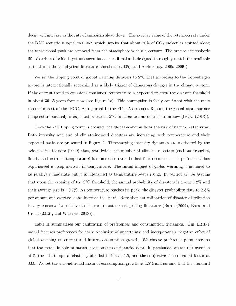
decay will increase as the rate of emissions slows down. The average value of the retention rate under

the BAU scenario is equal to 0.962, which implies that about 70% of CO2 molecules emitted along

the transitional path are removed from the atmosphere within a century. The precise atmospheric

life of carbon dioxide is yet unknown but our calibration is designed to roughly match the available

estimates in the geophysical literature (Jacobson (2005), and Archer (eg., 2005, 2009)).

We set the tipping point of global warming disasters to 2◦C that according to the Copenhagen

accord is internationally recognized as a likely trigger of dangerous changes in the climate system.

If the current trend in emissions continues, temperature is expected to cross the disaster threshold

in about 30-35 years from now (see Figure 1c). This assumption is fairly consistent with the most

recent forecast of the IPCC. As reported in the Fifth Assessment Report, the global mean surface

temperature anomaly is expected to exceed 2◦C in three to four decades from now (IPCC (2013)).

Once the 2◦C tipping point is crossed, the global economy faces the risk of natural cataclysms.

Both intensity and size of climate-induced disasters are increasing with temperature and their

expected paths are presented in Figure 2. Time-varying intensity dynamics are motivated by the

evidence in Raddatz (2009) that, worldwide, the number of climatic disasters (such as droughts,

floods, and extreme temperature) has increased over the last four decades — the period that has

experienced a steep increase in temperature. The initial impact of global warming is assumed to

be relatively moderate but it is intensified as temperature keeps rising. In particular, we assume

that upon the crossing of the 2◦C threshold, the annual probability of disasters is about 1.2% and

their average size is −0.7%. As temperature reaches its peak, the disaster probability rises to 2.8%

per annum and average losses increase to −6.0%. Note that our calibration of disaster distribution

is very conservative relative to the rare disaster asset pricing literature (Barro (2009), Barro and

Ursua (2012), and Wachter (2013)).

Table II summarizes our calibration of preferences and consumption dynamics. Our LRR-T

model features preferences for early resolution of uncertainty and incorporates a negative effect of

global warming on current and future consumption growth. We choose preference parameters so

that the model is able to match key moments of financial data. In particular, we set risk aversion

at 5, the intertemporal elasticity of substitution at 1.5, and the subjective time-discount factor at

0.99. We set the unconditional mean of consumption growth at 1.8% and assume that the standard

11

deviation of i.i.d. gaussian shocks is 1.6% per annum. We calibrate the dynamics of the long-run risk

component to match persistence of consumption growth in normal times. Consistent with the US

consumption data, in our specification the first-order autocorrelation of consumption growth absent

climate disasters is equal to 0.44. Exposure of the expected consumption growth to disaster risks is

set at 0.05. Note that while the average size of climate disasters in the expected growth component

is assumed to be quite modest, their effect on consumption is propagated due to persistence of

long-run risks. That is, upon a disaster, consumption growth does not immediately bounce back to

its normal level but is expected to remain low for a relatively long while.

The dynamics of future climate changes and their economic consequences are highly uncertain

and not yet well-understood. Pindyck (2007), and Heal and Millner (2014) provide a comprehensive

discussion of various sources of uncertainty in environmental economics. While some empirical

evidence on the impact of rising temperature and climatic disasters does exist (for example, Tol

(2002a, 2002b)), it is based on human experiences that have not yet been subjected to catastrophic

climate changes that we consider. Therefore, we can use it only as a guidance rather than a target.

Whenever possible, we calibrate the model parameters to be broadly consistent with assumptions

of the standard integrated assessment models and consensus forecasts outlined by the IPCC. With

this in mind, we do not intend to claim that our calibrated dynamics represent the future better

than others. We consider plausible dynamics and focus on highlighting the channels through which

beliefs about climate-change risks and risk preferences affect aggregate wealth. To discriminate

across the LRR-T model and alternative specifications, we confront each with financial market data

and empirical evidence on the impact of rising temperature on equity prices.

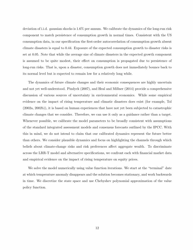
We solve the model numerically using value function iterations. We start at the “terminal” date

at which temperature anomaly disappears and the solution becomes stationary, and work backwards

in time. We discretize the state space and use Chebyshev polynomial approximation of the value

policy function.

12

3 Asset Pricing Implications of Temperature Risks

Different from the standard integrated assessment models, in which climate change is assumed to

cause a deterministic loss in future output or consumption, in our model, global warming affects

the economy through a risk channel. That is, climate change is a source of economic risk. Figure 3

displays the implications of global warming for the distribution of consumption growth. Notice that

because temperature-induced disasters are compensated, they have no effect on the ex-ante mean

of log consumption growth. This is similar to gaussian i.i.d. and long-run risks — ex-ante, global

warming does not affect the log level of future consumption path but does affect its variation, i.e.,

risk. As Panel (a) shows, climate-change driven disasters increase the ex-ante variation of future

growth. In our calibration, at the peak of temperature anomaly, the ex-ante annualized volatility

of cumulative consumption growth is about 0.18% higher compared with a no-disaster economy

(in relative terms this corresponds to more than ten percent increase in volatility). Also, because

global-warming disasters represent tail risks, the distribution of future consumption growth is both

negatively skewed and fat-tailed. Panel (b) of Figure 3 presents a side-by-side comparison of the

distribution of the normalized consumption growth at the peak of climate-driven disasters and the

corresponding distribution in the economy with no disasters.

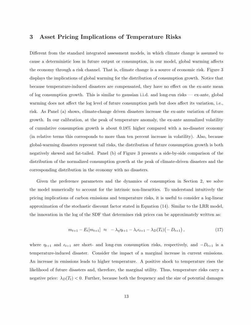
Given the preference parameters and the dynamics of consumption in Section 2, we solve

the model numerically to account for the intrinsic non-linearities. To understand intuitively the

pricing implications of carbon emissions and temperature risks, it is useful to consider a log-linear

approximation of the stochastic discount factor stated in Equation (14). Similar to the LRR model,

the innovation in the log of the SDF that determines risk prices can be approximately written as:

mt+1 − Et[mt+1] ≈ − ληηt+1 − λϵϵt+1 − λD(Tt)(−Dt+1

), (17)

where ηt+1 and ϵt+1 are short- and long-run consumption risks, respectively, and −Dt+1 is a

temperature-induced disaster. Consider the impact of a marginal increase in current emissions.

An increase in emissions leads to higher temperature. A positive shock to temperature rises the

likelihood of future disasters and, therefore, the marginal utility. Thus, temperature risks carry a

negative price: λD(Tt) < 0. Further, because both the frequency and the size of potential damages

13

depend on the level of temperature, so does the magnitude of the price of temperature risks. That

is, the price of temperature risk rises as temperature climbs up: ∂λD(Tt)∂Tt

< 0. Panel (a) of Figure 4

shows the elasticity of the stochastic discount factor to a one-percent increase in time-0 emissions.

As the figure shows, the marginal utility increases in response to higher emissions, and the increase

in marginal utility is amplified with temperature — the higher the temperature, the larger the

response of the marginal utility, i.e., the larger the price of temperature risks.

The premium for temperature risks is determined by their price and an asset exposure to

temperature fluctuations. Consider the return on aggregate wealth. Using log-linearization, we

can write the innovation in the log return, rt+1, as a sum of innovations in consumption growth and

the wealth to consumption ratio, i.e.,

rt+1 − Et[rt+1] ≈(∆ct+1 − Et[∆ct+1]

)+

(zt+1 − Et[zt+1]

), (18)

where zt+1 ≡ log(Zt) is the log of the aggregate wealth-consumption ratio.10 As Equation (18) shows,

exposure of wealth return to temperature risks depends on the impact of temperature fluctuations

on consumption growth and aggregate wealth. In our model, climate change is assumed to cause

disasters in consumption that become more severe as temperature keeps rising (see Equation (4)).

Under a preference for early resolution of uncertainty, that is, when risk aversion is larger than

the reciprocal of intertemporal elasticity of substitution, the impact of temperature fluctuations on

aggregate wealth is also negative. The elasticity of the wealth-consumption ratio to a marginal

increase in current emissions and and temperature is presented in Panel (b) of Figure 4. As the

figure shows, the wealth-consumption ratio falls in response to an increase in temperature. Thus, the

temperature beta of the aggregate wealth return (i.e., the projection coefficient of the asset return

on temperature shock) is negative and is increasing in magnitude with temperature. Recall that

temperature risk has a negative market price; hence, the product of the temperature beta and its

price that determines the temperature risk premium is positive. Higher emissions and temperature

raise temperature risk premia and future discount rates and lead to a decline in the wealth to

consumption ratio and asset valuations.

10This is similar to the innovation in an equity return, which is approximately equal to a sum of innovations individend growth and the price to dividend ratio.

14

To explore the implications of risk preferences for the joint dynamics of asset prices and

temperature, we consider two alternative specifications: (1) preferences for early resolution of

uncertainty, which we refer to as “Pref for ERU”, and (2) constant relative risk aversion preferences

that we refer to as “Power Utility”. To facilitate the comparison, we simplify consumption dynamics

by shutting off the long-run risk component and assuming that global warming affects only realized

consumption growth. Under these dynamics, climate risks continue to have a permanent negative

impact on consumption level but are assumed to have no effect on future economic growth. The

calibration of the two alternative specifications is summarized in Table II.

Figure 5 shows the response of aggregate wealth-consumption ratio to a one-percent increase in

current emissions under the two preference specifications. Similar to our baseline LRR-T model,

under preferences for early resolution of uncertainty, higher emissions lead to an increase in discount

rates and a fall in asset valuations. In contrast, in the power-utility economy with risk aversion larger

than one, discount rates decline in response to higher emissions and higher temperature (due to a

significant decline in risk-free rates) and asset prices feature a positive elasticity to temperature risks.

That is, under power utility, the wealth-consumption ratio rises when disasters are expected to be

more frequent and economic losses are expected to be larger.11 The implications of temperature

for the wealth to consumption ratio and equity valuations (price-dividend ratios) are important in

identifying the role of temperature risks.

The response of asset prices to temperature fluctuations in our baseline LRR-T model and

under the two alternative specifications is summarized in Table III. For each specification, we

simulate 50,000 paths of emissions, temperature and consumption and solve for the price of the

consumption claim. Temperature elasticities of asset prices are estimated by regressing the log of

the price-consumption ratio on temperature controlling for the relevant state variables. As the table

shows, under recursive preferences, asset valuations fall in response to an increase in temperature. In

particular, in the LRR-T model, a 0.5◦C increase in temperature (which corresponds to one standard

deviation of the empirical distribution) lowers the price of the consumption claim by about 0.87%. If

we account for market leverage of around three, the response of equity prices to temperature shocks

11The power-utility agents are still worse off since their utility is inversely related to wealth, but because the elasticityof utility to wealth is quite low, the decline in utility is very tiny, more than three orders of magnitude smaller thanthe corresponding decline under recursive preferences.

15

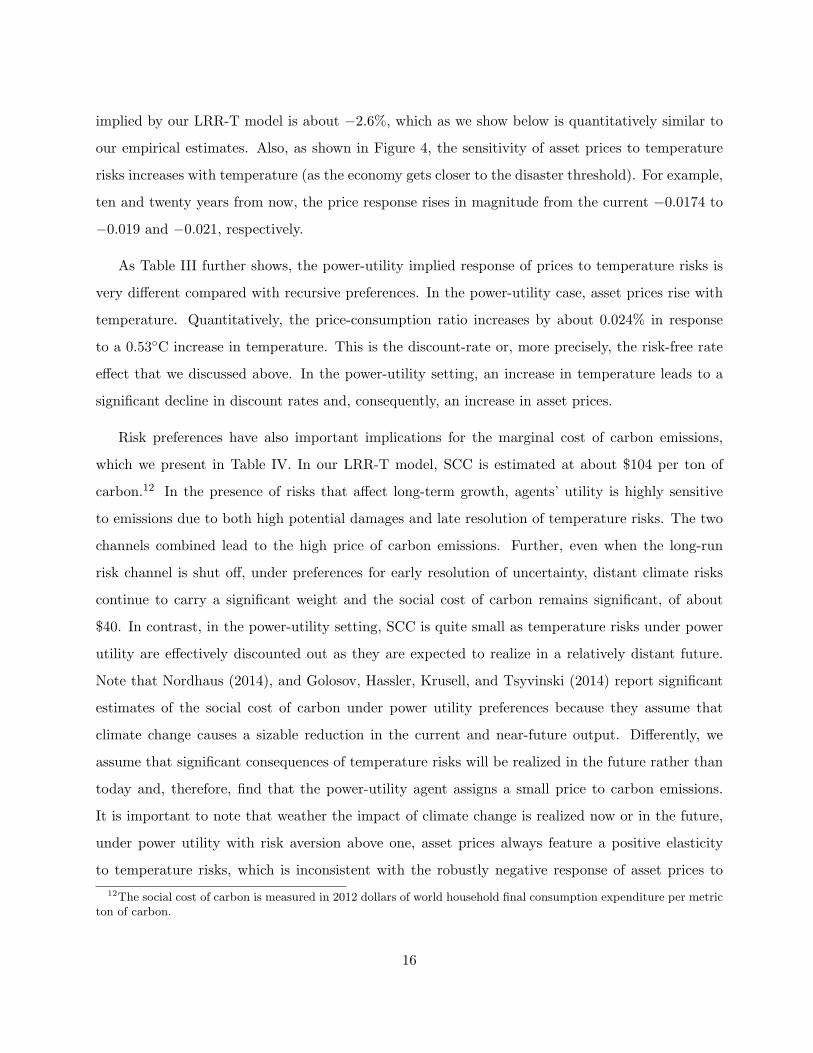
implied by our LRR-T model is about −2.6%, which as we show below is quantitatively similar to

our empirical estimates. Also, as shown in Figure 4, the sensitivity of asset prices to temperature

risks increases with temperature (as the economy gets closer to the disaster threshold). For example,

ten and twenty years from now, the price response rises in magnitude from the current −0.0174 to

−0.019 and −0.021, respectively.

As Table III further shows, the power-utility implied response of prices to temperature risks is

very different compared with recursive preferences. In the power-utility case, asset prices rise with

temperature. Quantitatively, the price-consumption ratio increases by about 0.024% in response

to a 0.53◦C increase in temperature. This is the discount-rate or, more precisely, the risk-free rate

effect that we discussed above. In the power-utility setting, an increase in temperature leads to a

significant decline in discount rates and, consequently, an increase in asset prices.

Risk preferences have also important implications for the marginal cost of carbon emissions,

which we present in Table IV. In our LRR-T model, SCC is estimated at about $104 per ton of

carbon.12 In the presence of risks that affect long-term growth, agents’ utility is highly sensitive

to emissions due to both high potential damages and late resolution of temperature risks. The two

channels combined lead to the high price of carbon emissions. Further, even when the long-run

risk channel is shut off, under preferences for early resolution of uncertainty, distant climate risks

continue to carry a significant weight and the social cost of carbon remains significant, of about

$40. In contrast, in the power-utility setting, SCC is quite small as temperature risks under power

utility are effectively discounted out as they are expected to realize in a relatively distant future.

Note that Nordhaus (2014), and Golosov, Hassler, Krusell, and Tsyvinski (2014) report significant

estimates of the social cost of carbon under power utility preferences because they assume that

climate change causes a sizable reduction in the current and near-future output. Differently, we

assume that significant consequences of temperature risks will be realized in the future rather than

today and, therefore, find that the power-utility agent assigns a small price to carbon emissions.

It is important to note that weather the impact of climate change is realized now or in the future,

under power utility with risk aversion above one, asset prices always feature a positive elasticity

to temperature risks, which is inconsistent with the robustly negative response of asset prices to

12The social cost of carbon is measured in 2012 dollars of world household final consumption expenditure per metricton of carbon.

16

temperature fluctuations in the data that we document and discuss below.

Temperature risks aside, our LRR-T model corresponds to the long-run risks model of Bansal

and Yaron (2004). As they show, with preferences for early resolution of uncertainty, risks that

matter for the long run carry high risk premia and are able to account for the dynamics of equity

prices and asset returns. Our calibration of the gaussian part of consumption dynamics is similar

to theirs and, therefore, is consistent with financial market data. As Table IV shows, the average

risk-free rate in the LRR-T specification is 0.9%, and the risk premium on consumption claim is

about 1.7%. Hence, the implied equity premium, assuming leverage of 3, is about 5% per annum. It

is important to emphasize that most of the risk premium is the compensation for long-run gaussian

risks, and only a relatively modest fraction of the overall premium is due to temperature risks.

4 Temperature and Asset Prices: Evidence from the US Markets

In our model, rising temperature increases economic risk and thus has a negative effect on the

macro-economy. Further, with a preference for early resolution of uncertainty, higher temperature

leads to a decline in aggregate wealth and asset prices. The empirical research on the impact of

global warming on the macro-economy has primarily focused on the effect of temperature on growth.

For example, Dell, Jones, and Olken (2012) analyze the impact of rising temperature on output and

find evidence that current output and short-term future growth tend to decrease with temperature,

although the negative effect seems to be entirely concentrated in low-income countries. Motivated

by our model, we take a different approach and measure the impact of temperature on the macro-

economy using forward-looking equity prices rather than past growth rates. Long-horizon equity

prices reflect information about future expected growth rates and future risks. If temperature is

expected to affect future growth and/or risk, these expectations ought to be reflected in capital

markets provided that agents care about the future. Note that if past and current growths have not

yet been exposed to catastrophic temperature risks, it would not be possible to detect the impact of

temperature from the available output data. In contrast to backward-looking output growth rates,

equity prices reveal agents’ expectations about the future and, thus, contain information about a

potential impact of temperature on the economy. This is the idea that we pursue in our empirical

17

analysis of equity prices and temperature fluctuations.

Although, for simplicity, in the theory section we consider the economy in aggregate without

explicitly modeling its sectors or markets, the cross-sectional implications of our model are

straightforward. Assets that are highly exposed to temperature risks should carry higher risk

premia relative to assets with lower sensitivity. We exploit this prediction to measure the impact of

temperature fluctuations on equity prices and to estimate the price of temperature risks.

4.1 US Data

We use two data sets from the US equity markets: the standard set of 25 portfolios sorted by market

capitalization and book-to-market ratio and a set of industry portfolios.13 Following the classification

of the National Institute for Occupational Safety and Health (NIOSH) and Graff Zivin and Neidell

(2014), we construct ten industry portfolios that represent high and low heat-exposed sectors of the

US economy. The first group comprises mining, oil and gas extraction, construction, transportation,

and utilities — industries that operate in hot and humid environments. The remaining sectors:

manufacturing, wholesale, retail trade, services, and communications, are classified as sectors with

low exposure to heat.14 To control for market and consumption risks, we use the CRSP value-

weighted portfolio of all stocks traded on the NYSE, AMEX, and NASDAQ and per-capita series

of real consumption expenditure on non-durables and services from the NIPA tables available from

the Bureau of Economic Analysis. Excess returns are constructed by subtracting the CRSP risk-

free rate series from portfolio returns. Temperature data for the contiguous US are measured in

degrees Fahrenheit and come from the National Oceanic and Atmospheric Administration of the

US Department of Commerce. The data are sampled at the annual frequency and span the period

from 1934 to 2014.

13Book-to-market and size sorted portfolio data are obtained from Kenneth French’s online data library.14We are unable to consider the agricultural sector because a portfolio of public agricultural firms is extremely thin

— on average, it contains about 9 firms and in the first part of the sample it comprises only 1-2 firms. Firms in thefinancial section are excluded.

18

4.2 Temperature Betas

We measure equity exposure to temperature risks by regressing portfolio excess returns on

temperature variations controlling for market and economic growth risks, specifically:

Rei,t = ai + βi,∆T ∆TKt + βi,MReM,t + βi,CξC,t + ui,t , (19)

where Rei,t is the excess return of portfolio i, ∆TKt is the K-year change in temperature, ReM,t is

the excess return of the market portfolio, and ξC,t is the innovation in the two-year moving-average

of aggregate consumption growth that proxies for persistent variations in macro-economic growth

(as in Parker and Julliard (2005), Bansal, Dittmar, and Lundblad (2005)). Our controls for market

and consumption risks are motivated by our theoretical model, and the equilibrium CAPM and

consumption-based CAPM frameworks of Sharpe (1964), Lucas (1978), and Breeden (1979).

To differentiate between low-frequency temperature shocks that contribute to global warming

and short-term fluctuations in temperature that correspond to variations in weather, we consider

different horizons K’s ranging from one to ten years. Note that when K = 1, ∆TKt ≡ ∆T , which

corresponds to annual (short-run) fluctuations in weather. When K ≫ 1, ∆TKt represents long-run

temperature risks that are associated with global warming. In essence, by averaging temperature

variations over time, we filter out short-run weather fluctuations and isolate shocks to the low-

frequency component (i.e., temperature trend). Our empirical evidence is similar if, instead, we

construct temperature trend using the Hodrick and Prescott (1997) filter.15 Also, our evidence

remains virtually the same if we use innovations in the long-run change of temperature instead of

first differences. The advantage of using first differences is that they are observable and, thus, are

not subject to estimation errors.

Figure 6 presents a scatter plot of average excess returns and temperature betas, βi,∆T , for 25

book-to-market and size sorted portfolios and ten industry portfolios. Panel (a) shows exposure to

annual change in temperature, and Panel (b) presents betas with respect to variations in the five-

year change in temperature. Note that with only few exceptions, equity portfolios have negative

15Note that the Hodrick and Prescott (1997) filter is a two-sided filter and, hence, it is constructed using futuretemperature data. The first differences that we use are not subject to look-ahead biases because they are measuredusing the already available, current and past, temperature data.

19

elasticity to temperature fluctuations. That is, equity prices tend to decline in response to an

increase in temperature. Notice also that portfolios that carry high premia feature high sensitivity

to low-frequency temperature risks, which suggests that temperature risks carry a negative price.

The magnitudes of long-run temperature betas corresponding to the five-year horizon are

reported Table V. As Panel A shows, while almost all book-to-market and size sorted portfolios

feature a negative response to long-run temperature risks, their exposure is not homogenous. In

particular, high book-to-market firms tend to have much higher (i.e., more negative) exposure

to temperature fluctuations relative to low book-to-market firms. Empirical evidence in Bansal,

Dittmar, and Lundblad (2005), Hansen, Heaton, and Li (2008), and Bansal, Kiku, Shaliastovich,

and Yaron (2014) shows that high book-to-market firms are much more sensitive to persistent growth

risks compared with low book-to-market firms, which accounts for the cross-sectional differences

in temperature exposure that we document. According to our LRR-T model, an increase in

temperature trend raises the likelihood of growth diasters in the long run; therefore, assets that

are highly exposed to persistent growth risks also feature high sensitivity to long-run temperature

risks.

The variation in temperature betas across industry portfolios, presented in Panel B of Table V,

is fairly consistent with NIOSH classification. Only with the exception of wholesale, industries that

are classified as low heat-exposure sectors have small positive sensitivity to temperature variation,

whereas firms in high heat-exposure sectors have negative elasticity to temperature risks. In

unreported results, we confirm that the differences between the two industry groups are strongly

significant particularly when temperature risks are measured at low frequencies (i.e., beyond one-

year horizon). In the next section, we explore the pricing implications of temperature risks.

4.3 Price of Temperature Risk

We estimate the price of temperature risks using efficient GMM of Hansen (1982) by exploiting

the Euler condition for a cross-section of equity returns. We consider the following linear SDF

20

specification:

E[Rei,t

(1− E[Mt] +Mt

)]= 0, for i = 1, .., N , (20)

Mt = −λ∆T∆TKt − λMreM,t − λCξC,t , (21)

where λ∆T , λM and λC denote prices of temperature, market and consumption growth risks,

respectively. We remove the mean of the SDF as it is not identified because equity portfolios

are measured in excess returns. Note that our estimation approach is equivalent to a GLS cross-

sectional regression of equity premia on the covariance between returns and factors that imposes a

zero intercept. To keep the number of portfolios manageable, we estimate risk prices using industry

portfolios and a subset of book-to-market and size sorted portfolios. In particular, for each size

cohort, we use three portfolios with low, median and high book-to-market characteristic. Thus, in

total, the cross-section comprises 15 book-to-market/size and 10 industry sorted portfolios.

Table VI reports the GMM estimates of the price of temperature risks, λ∆T , across different

horizons varying from one to ten years. Consistent with the prediction of our model, we find that

the price of temperature risks is significantly negative, particularly when temperature risks are

measured at low frequencies. For example, variations in three- and ten-year temperature trends are

priced at −0.51 and −0.46, respectively, with the corresponding t-statistics of −2.25 and −3.19.

Because equity portfolios, on average, have negative temperature exposure, temperature risks carry

positive premium in equity markets. Further, assets that are more exposed to temperature risks,

such as value firms and firms in high heat-exposure industries, have higher premia relative to their

counterparts. For example, our estimates suggest that value firms, on average, provide a 1.2%

premium as a compensation for their exposure to long-run temperature risks, whereas growth firms

carry about −0.9% temperature premium because they provide insurance against low-frequency

temperature fluctuations. The average long-run temperature premium in high and low heat-exposed

sectors are 1% and −0.5%, respectively. As the bottom panel of Table VI shows, our linear model

specification is not rejected by the χ2-test of overidentifying restrictions.

It is important to note that temperature fluctuations are exogenous relative to a long list of

reduced-form return-based factors that are popular in empirical asset pricing. Therefore, while we

21

control for market and economic growth risks (as motivated by the model), we do not include any

ad-hoc empirical factors in our regression specifications. Further, to ensure that our evidence is not

simply due to a lucky draw, we run the following simulation experiment. We generate temperature

series of the sample size that matches the data and replace the observed temperature with the

simulated draw. We then estimate the price of temperature risks using simulated temperature

series as we do in the actual data. We repeat this simulation exercise 10,000 times and construct a

Monte Carlo distribution of t-statistics under the null that temperature variations carry a zero price.

We find that across virtually all horizons, t-statistics for the estimate of the price of low-frequency

temperature risks are in the bottom fifth percentile of the null distribution. That is, if temperature

risks had no impact on equity valuations, it would be highly unlikely to observe the evidence that

we document.

4.4 Time-Varying Price of Temperature Risk

As discussed in Section 3, our model predicts that the risk premium for temperature fluctuations

increases with temperature as the impact of climate change on the economy intensifies. Motivated by

the model’s implications, we take into account potential variation in the conditional risk premium

and parameterize the dynamics of the price of temperature risks to be a linear function of the

temperature trend. That is, we consider the following specification of the stochastic discount factor:

Mt = −(λ∆T + λT ·∆TT

Kt−1

)∆TKt − λMr

eM,t − λCξC,t , (22)

where TK

is the K-year moving average trend in temperature.

The GMM estimates of λ∆T and λT ·∆T are presented Table VII. Our evidence reveals that the

price of long-run temperature risks that contribute to global warming has risen over time along with

the rise in temperature. As the table shows, the estimates of the time-varying component of the

price of temperature risks are negative and strongly significant at long horizons. For example, at

the ten-year horizon, λT ·∆T is −0.77 with the t-statistics of −2.97.

The negative coefficient on the scaled temperature factor implies that the premium for

temperature risks has been increasing with the level of temperature as predicted by our model. The

22

magnitude and the dynamics of the risk premium for low-frequency temperature fluctuations are

presented in Figure 7. The figure shows the temperature premium of an average equity portfolio with

median size and book-to-market characteristics based on the estimates reported in Table VII that

correspond to the ten-year horizon. A median equity exposure to low-frequency temperature risks

carries a premium of around 0.4%, on average, which as the figure shows, has increased significantly

since mid-80’s reaching about 1% at the end of the sample.

5 Temperature and Asset Prices: Evidence from Global Markets

In this section, we evaluate the impact of temperature risks on equity valuations using panel data

from global financial markets. Because the span of the available international data is relatively

short, we measure the impact of temperature fluctuations by pooling the data and simultaneously

exploiting time-series and cross-sectional variation in country-level temperature and equity prices.

Also, because historically international markets are not fully integrated and different countries

feature different degrees of segmentation and frictions, we limit our attention on understanding the

overall impact of temperature fluctuations on asset valuations.

5.1 Data

We use country-level panel data that cover 39 countries and span the time period from 1970 and

2012. Country-level and global temperature that correspond to land-surface temperature anomaly

are taken from the Berkeley Earth open database. Temperature anomaly is measured in degrees

Celsius and is defined relative to the 1951-1980 average. The price-dividend data come from the

Global Financial Data and provide a market proxy for the wealth-to-consumption ratio. We also

collect market equity returns for each country in our sample. Country-specific macro data (such

as gross domestic product, inflation, unemployment, real interest rates) are taken from the World

Bank database and are available for the 1980-2009 period. The list of 39 countries is provided in

Table VIII. This is the most exhaustive set with reliable capital market data that we could find, as

such, it is tilted towards developed economies as they are more likely to have a history of equity

markets.

23

In our sample, 38 out of 39 countries have experienced a significant increase in temperature

over the sample period. The median temperature anomaly across countries is about 0.38◦C and

over the last decade, between 2003 and 2012, the anomaly averages 0.73◦C . Figure 8 shows the

histogram of the temperature anomaly in the most recent decade in our sample. We find that

local temperature series have a strong common component that is highly correlated with variation

in global temperature. Using the cross-section of countries we carry out a principal component

analysis on the country-level temperature data. We find that the first principal component of annual

temperature series accounts for about 53% of the total variation in temperature across countries

and has a 71% correlation with global temperature anomaly. At low frequencies, the co-movement

in local temperature becomes much stronger. For example, using five-year moving-averages of local

temperature, we find that the first principal component explains about 81% of the overall variation

in local temperature trends. This evidence suggests that systematic climate risk is most likely

driven by low-frequency temperature risks (i.e., risks associated with global warming) rather than

by weather or short-run temperature fluctuations.

Our analysis of equity prices reveals a strong low dimensional factor structure also in price-

dividend ratios. We find that the first principal component extracted from the cross-section of

price-dividend ratios accounts for about 69% of the total variation in prices across countries and

the second component explains an additional 10%. This suggests that the cross-country variation

in equity valuations is influenced by common global macro-economic factors. Jagannathan and

Marakani (2015) show that the first two price-dividend ratio factors provide robust proxies for

future economic growth and variation in macro-economic uncertainty. Guided by their evidence, we

use the first two principal components to control for global macro-economic risks in our regression

analysis. Our empirical approach is conservative as we ask if, after controlling for global and local

macro-risk factors, long-run fluctuations in temperature have any effect on equity valuations.

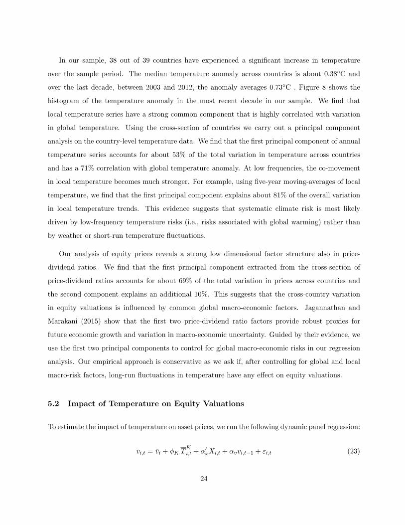
5.2 Impact of Temperature on Equity Valuations

To estimate the impact of temperature on asset prices, we run the following dynamic panel regression:

vi,t = vi + ϕK TKi,t + α′

xXi,t + αvvi,t−1 + εi,t (23)

24

where vi,t is the log of the equity price-dividend ratio of country i at date t, vi is the country-specific

fixed effect, TKi,t is a K-year moving-average of local temperature, and Xi,t is a set of controls

that captures the effect of global and local risks on asset prices, i.e., macro-economic risks that

are distinct from temperature. We vary K between one and five years and do not consider longer

horizons because of a relatively short span of panel data.16 We control for common global macro-

economic variations using two price-dividend ratio factors.17 The set of local controls comprises

country-specific inflation, unemployment, real interest rate, and growth in gross domestic product

(gdp). The remaining persistence in asset prices is absorbed by the lagged country-specific price-

dividend ratio. We estimate the parameters using the Arellano and Bond (1991)’s GMM estimator

applied to the first-differenced data and use the White (1980)’s robust estimator of the variance-

covariance matrix.

Our focus is on parameter ϕK that measures sensitivity of equity prices to local temperature

variations. The estimates of temperature elasticities for the full sample are reported in “1980-2009”

rows of Table IX. We find that at both short and long horizons, temperature risks have a significant

negative effect on equity valuations. The estimated elasticities vary between −0.076 (t-stat = −4.41)

at the short horizon and −0.105 (t-stat = −3.33) at the long horizon. To interpret the magnitude

of the estimates, note that ϕK measures semi-elasticity of asset prices to temperature fluctuations.

Hence, a one standard-deviation increase in annual temperature anomaly of around 0.5◦C leads to

about 3.8% decline in equity valuations. The impact of low-frequency temperature risks is similar;

for example, a one standard-deviation increase in the five-year temperature trend lowers equity

valuations by about 3.4%.

In Table IX we also explore if the effect of temperature on the economy has changed across time.

Ideally, to uncover such changes, we would want to compare temperature elasticities measured over

earlier and more recent sample periods. This, however, is not entirely feasible given the fairly short

span of the available data. Therefore, to explore time-variation in elasticities we estimate them using

overlapping samples. We start with the early 1980-2000 sample and then progressively increase the

16Given the limited availability of the country-specific controls, the panel regression is estimated on a subsample of34 countries over the 1980-2009 period.

17To allow global macro risks have differential effect across countries, we also include the interaction of the twoprincipal components with country-income dummies. While the estimates on the interaction terms are mostlysignificant, their inclusion has virtually no effect on the estimated elasticity of equity prices to temperature risksand its significance. Therefore, for parsimony, we report evidence based on the specification with no interaction terms.

25

sample end to 2005 and 2009 by adding more recent data. Our estimates show that the effect of

temperature on equity valuations has risen considerably over time. At the one-year horizon, the

point estimates change from −0.016 in the early sample to −0.076 in the full sample. Similarly, the

price impact of temperature risks measured at lower frequencies (i.e., for K>1) more than doubles

when more recent data are incorporated in estimation. This evidence suggests that as temperature

rises, global warming imposes higher risks on the economy and, therefore, leads to a larger decline

in wealth. As discussed above, our model is consistent with this evidence — in the model, rising

temperature increases the size and the probability of disasters over time, leading to a steeper decline

in aggregate wealth.

In our panel regression setting we measure the economic impact of temperature risks by exploiting

both time-series and cross-sectional variation in temperature. Local temperature series, especially

their low-frequency fluctuations, feature a strong common (global) component. Replacing local

temperature series in regression specification in Equation (23) with global temperature, we find

that global temperature risks have also a strongly significant negative effect of equity prices. This

evidence (which is available upon request) suggests that the negative elasticity of equity valuations

to local temperature risks is largely due to common time-series variation in temperature across

countries.

5.3 Long-Run vs. Short-Run Temperature Risks

To better understand which risks, short-run (i.e., weather-type) risks or long-run temperature

variations associated with global warming, matter more we consider the following panel regression:

vi,t = vi + ϕLR LRKi,t + ϕSR SRi,t + α′

xXi,t + αvvi,t−1 + εi,t , (24)

where LRKi,t proxies for low-frequency temperature risks and is measured by the K-year moving-

average of local temperature, for K = {3, 5}, and SRi,t is annual temperature orthogonalized with

respect to long-run fluctuations. We orthogonalize short- and long-run temperature variations in

order to identify their separate effects. The estimates of long- and short-run elasticities, ϕLR and

ϕSR, are presented in Table X.

26

Consistent with the evidence discussed above, we find a negative and statistically significant

response of equity valuations to low-frequency variations in temperature. We also find that once

we control for long-run fluctuations in temperature, short-run temperature risks tend to also have a

negative effect on equity prices, however, its magnitude is generally small and not as significant. In

unreported results, we also estimate exposure of equity returns to long- and short-run temperature

risks and similarly find statistically negative betas with respect to low-frequency risks and generally

insignificant exposure to short-run variations in temperature. Our evidence thus suggests that the

negative impact of temperature on the economy is mostly driven by its low-frequency (i.e., trend)

risks that correspond to global warming.

To further examine the impact of long- and short-run temperature risks on equity prices, we

estimate their joint dynamics using a first-order vector-autoregression (VAR). Specifically, we exploit

the following panel VAR specification:

Yi,t = ai +AYi,t−1 + bXt + ui,t (25)

where Yi,t = (T8i,t, Ti,t, vi,t)

′ is a vector of the eight-year moving-average of local temperature, the

annual temperature series and the price-dividend ratio of country i. We include country fixed effects

(ai) and use the two price-dividend ratio factors to control for global risks (Xt denotes the vector

of global controls). We estimate the VAR using the full sample of panel data from 1970 until 2012

and, therefore, we able to consider a relatively long horizon of eight years to measure low-frequency

temperature risks. The VAR-regression output is reported in Table XI, and in Figure 9 we plot

the implied impulse responses of equity prices to a one-standard deviation shock in temperature

trend (T8i,t) and a one-standard deviation innovation in annual temperature (Ti,t). The shaded area

around the estimated responses represents the two standard-error band. As Panel (a) shows, the

VAR-based response of equity prices to low-frequency temperature risks is significantly negative.

Notice also that the effect of trend shocks is quite persistent — an increase in temperature trend

leads to a decline in equity prices on impact and in the long run. Similar to the evidence presented

above, short-run temperature fluctuations do not seem to have a sizable effect. In all, our empirical

evidence suggests that climate change measured by a long-term increase in temperature has a

significant negative impact on the world economies.

27

6 Conclusion

Using capital market data, we show that temperature risks have a significant negative effect on

wealth. An increase in temperature, especially at low frequencies, lowers equity valuations around

the globe and in the US markets. To understand the implications of persistent temperature risks and

to guide our empirical analysis, we model the dynamic interaction between economic growth and

climate change. We show that even if the real effect of rising temperature is deferred into the future,

its wealth effect is realized today. That is, even if global warming increases uncertainty or lowers

expectations about growth in a relatively distant future, under preferences for early resolution of

uncertainty, it leads to an immediate decline in wealth and equity valuations. Hence, forward-looking

capital markets might provide valuable information about the economic impact of temperature risks

— information that might not be possible to learn from the past (backward-looking) income growth

data. We explore this idea in our empirical work. Consistent with our model’s predications, we

find that low-frequency temperature risks have a significant negative effect on equity valuations and

carry a positive premium in equity markets. We also show that the premium for low-frequency

temperature risks that contribute to global warming has been increasing over time along with the

rise in temperature.

28

References

Anthoff, David, and Richard S.J. Tol, 2012, The Climate Framework for Uncertainty, Negotiation

and Distribution (FUND), Working paper, Technical Description, Version 3.6.

Anthoff, David, and Richard S.J. Tol, 2013, The Uncertainty about the Social Cost of Carbon: A

Decomposition Analysis using FUND, Climatic Change 117, 515–530.

Archer, David, 2005, Fate of Fossil Fuel CO2 in Geologic Time, Journal of Geophysical Research:

Oceans 110, C09S05.

Archer, David, 2009, Atmospheric Lifetime of Fossil Fuel Carbon Dioxide, Annual Review of Earth

and Planetary Sciences 37, 117–134.

Arellano, Manuel, and Stephen Bond, 1991, Some Tests of Specification for Panel Data: Monte

Carlo Evidence and an Application to Employment Equations, Review of Economic Studies 58,

277–297.

Bansal, Ravi, Robert Dittmar, and Christian Lundblad, 2005, Consumption, Dividends, and the

Cross-Section of Equity Returns, Journal of Finance 60, 1639–1672.

Bansal, Ravi, Dana Kiku, and Marcelo Ochoa, 2015, Climate Change and Growth Risks, Working

paper, Duke University.

Bansal, Ravi, Dana Kiku, Ivan Shaliastovich, and Amir Yaron, 2014, Volatility, the Macroeconomy

and Asset Prices, Journal of Finance 69, 2471–2511.

Bansal, Ravi, Dana Kiku, and Amir Yaron, 2010, Long-Run Risks, the Macroeconomy, and Asset

Prices, American Economic Review: Paper & Proceedings 100, 542–546.

Bansal, Ravi, and Marcelo Ochoa, 2012, Temperature, Aggregate Risk, and Expected Returns,

Working paper, Duke University.

Bansal, Ravi, and Amir Yaron, 2004, Risks for the Long Run: A Potential Resolution of Asset

Pricing Puzzles, Journal of Finance 59, 1481–1509.

29

Barro, Robert J., 2009, Rare Disasters, Asset Prices, and Welfare Costs, American Economic Review

99, 243–264.

Barro, Robert J., and Jose F. Ursua, 2012, Rare Macroeconomic Disasters, Annual Review of

Economics 4, 83–109.

Borovicka, Jaroslav, and Lars P. Hansen, 2014, Examining Macroeconomic Models through the Lens

of Asset Pricing, Journal of Econometrics 183, 67–90.

Breeden, Douglas T., 1979, An intertemporal asset pricing model with stochastic consumption and

investment opportunities, Journal of Financial Economics 7, 265–296.

Dell, Melissa, Benjamin F. Jones, and Benjamin A. Olken, 2012, Temperature Shocks and Economic

Growth: Evidence from the Last Half Century, American Economic Journal: Macroeconomics

4(3), 66–95.

Epstein, Larry G., and Stanley E. Zin, 1989, Substitution, Risk Aversion, and the Intertemporal

Behavior of Consumption and Asset Returns: A Theoretical Framework, Econometrica 57, 937–

969.

Gollier, Christian, 2012, Pricing the Planet’s Future: The Economics of Discounting in an Uncertain

World. (Princeton University Press).

Golosov, Mikhail, John Hassler, Per Krusell, and Aleh Tsyvinski, 2014, Optimal Taxes on Fossil

Fuel in General Equilibrium, Econometrica 82, 41–88.

Gourio, Francois, 2012, Disaster Risk and Business Cycles, American Economic Review 106, 2734–

2766.

Graff Zivin, Joshua, and Matthew Neidell, 2014, Temperature and the Allocation of Time:

Implications for Climate Change, Journal of Labor Economics 32, 126.

Hansen, Lars, 1982, Large Sample Properties of Generalized Methods of Moments Estimators,

Econometrica 50, 1009–1054.

Hansen, Lars Peter, John C. Heaton, and Nan Li, 2008, Consumption Strikes Back? Measuring

Long-Run Risk, Journal of Political Economy 116, 260–302.

30

Hansen, Lars P., and Thomas J. Sargent, 2006, Robust Control and Model Misspecification, Journal

of Economic Theory 128, 45–90.

Hansen, Lars P., and Jose A. Scheinkman, 2012, Pricing Growth-Rate Risk, Finance and Stochastics

16, 1–15.

Heal, Geoffrey, and Antony Millner, 2014, Uncertainty and Decision Making in Climate Change

Economics, Review of Environmental Economics and Policy.

Heutel, Garth, 2012, How Should Environmental Policy Respond to Business Cycles? Optimal

Policy Under Persistent Productivity Shocks, Review of Economic Dynamics 15, 244–264.

Hodrick, Robert J., and Edward C. Prescott, 1997, Postwar U.S. Business Cycles: An Empirical

Investigation Journal of Money, Credit, and Banking, Journal of Money, Credit, and Banking 29,

1–16.

Hope, Chris, 2011, The PAGE09 Integrated Assessment Model: A Technical Description, Working

paper, Cambridge Judge Business School.

IPCC, 2007, Climate Change 2007: Synthesis Report. (Geneva, Switzerland).

IPCC, 2013, Working Group I Contribution to the IPCC Fifth Assessment Report. Climate Change

2013: The Physical Science Basis. (Geneva, Switzerland).

Jacobson, Mark Z., 2005, Correction to “Control of Fossil-Fuel Particulate Black Carbon and

Organic Matter, Possibly the Most Effective Method of Slowing Global Warming”, Journal of

Geophysical Research: Atmospheres 110, D14105.

Jagannathan, Ravi, and Srikant Marakani, 2015, Price Dividend Ratio Factor Proxies for Long Run

Risks, Review of Asset Pricing Studies, forthcoming.

Kreps, David M., and Evon L. Porteus, 1978, Temporal Resolution of Uncertainty and Dynamic

Choice, Econometrica 46, 185–200.

Lemoine, Derek M., and Christian Traeger, 2012, Tipping Points and Ambiguity in the Integrated

Assessment of Climate Change, Working paper, National Bureau of Economic Research, #18230.

31

Lucas, Robert, 1978, Asset prices in an exchange economy, Econometrica 46, 1429–1446.

Nordhaus, William, 2014, Estimates of the Social Cost of Carbon: Concepts and Results from the

DICE-2013R model and Alternative Approaches, Journal of the Association of Environmental

and Resource Economists.

Nordhaus, William D., 2008, A Question of Balance: Weighing the Options on Global Warming

Policies. (Yale University Press).

Nordhaus, William D., 2010, Economic Aspects of Global Warming in a Post-Copenhagen

Environment, Proceedings of the National Academy of Sciences 107, 11721–11726.

Parker, Jonathan A., and Christian Julliard, 2005, Consumption risk and the cross-section of

expected returns, Journal of Political Economy 113, 185–222.

Pindyck, Robert S., 2007, Review of Environmental Economics and Policy, Uncertainty in

Environmental Economics 1, 45–65.

Pindyck, Robert S., 2012, Uncertain Outcomes and Climate Change Policy, Journal of

Environmental Economics and Management 63, 289–303.

Raddatz, Claudio, 2009, The Wrath of God: Macroeconomic Costs of Natural Disasters, Working

paper, World Bank Policy Research.

Rietz, Thomas A., 1988, The Equity Risk Premium: A Solution, Journal of Monetary Economics

22, 117131.

Sharpe, William, 1964, Capital asset prices: A theory of market equilibrium under conditions of

risk, Journal of Finance 19, 425–442.

Stern, Nicholas H., 2007, The Economics of Climate Change: The Stern Review. (Cambridge

University Press.).

Tol, Richard S.J., 2002a, New Estimates of the Damage Costs of Climate Change, Part I: Benchmark

Estimates, Environmental and Resource Economics 21, 47–73.

Tol, Richard S.J., 2002b, New Estimates of the Damage Costs of Climate Change, Part II: Dynamic

Estimates, Environmental and Resource Economics 21, 135–160.

32

Wachter, Jessica A., 2013, Can Time-Varying Risk of Rare Disasters Explain Aggregate Stock

Market Volatility?, Journal of Finance 68, 987–1035.

Weil, Philippe, 1990, Nonexpected Utility in Macroeconomics, Quarterly Journal of Economics 105,

29–42.

Weitzman, Martin L., 2009, On Modeling and Interpreting the Economics of Catastrophic Climate

Change, Review of Economics and Statistics 91, 1–19.

Weitzman, Martin L., 2010, What is the “Damages Function” for Global Warming – And What

Difference Might It Make?, Climate Change Economics 1, 57–69.

White, Halbert, 1980, A Heteroskedasticity-Consistent Covariance Matrix and a Direct Test for

Heteroskedasticity, Econometrica 48, 817838.

33

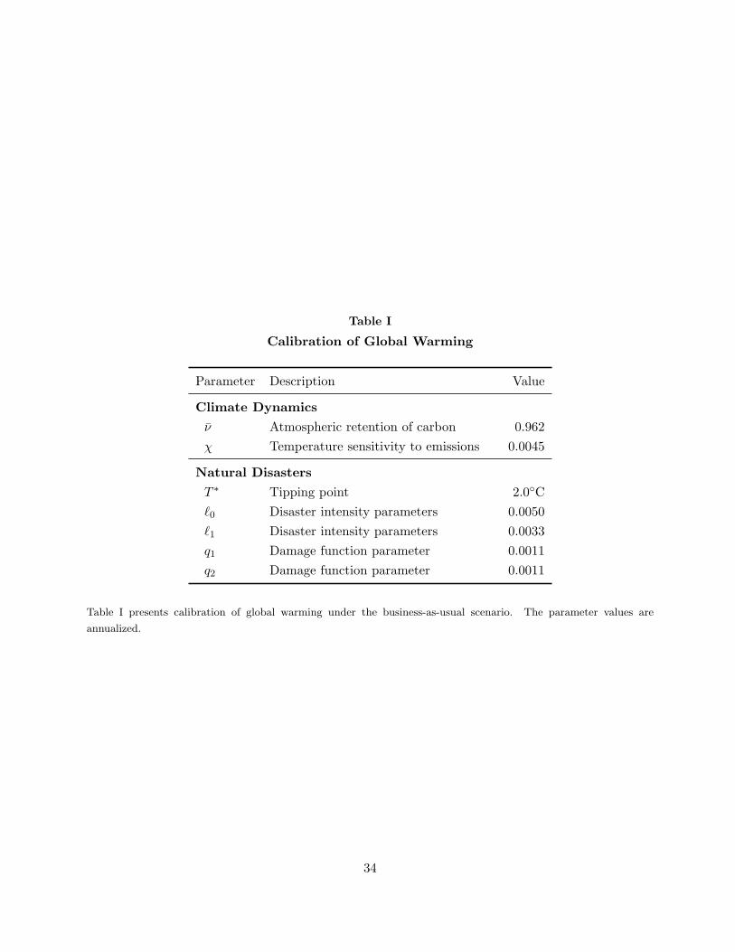
Table I

Calibration of Global Warming

Parameter Description Value

Climate Dynamics

ν Atmospheric retention of carbon 0.962

χ Temperature sensitivity to emissions 0.0045

Natural Disasters

T ∗ Tipping point 2.0◦C

ℓ0 Disaster intensity parameters 0.0050

ℓ1 Disaster intensity parameters 0.0033

q1 Damage function parameter 0.0011

q2 Damage function parameter 0.0011

Table I presents calibration of global warming under the business-as-usual scenario. The parameter values are

annualized.

34

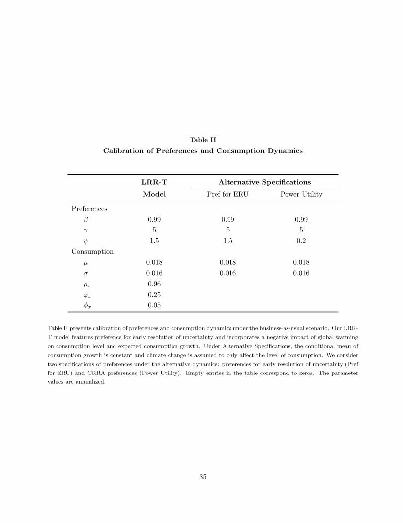
Table II

Calibration of Preferences and Consumption Dynamics

LRR-T Alternative Specifications

Model Pref for ERU Power Utility

Preferences

β 0.99 0.99 0.99

γ 5 5 5

ψ 1.5 1.5 0.2

Consumption

µ 0.018 0.018 0.018

σ 0.016 0.016 0.016

ρx 0.96

φx 0.25

ϕx 0.05

Table II presents calibration of preferences and consumption dynamics under the business-as-usual scenario. Our LRR-

T model features preference for early resolution of uncertainty and incorporates a negative impact of global warming

on consumption level and expected consumption growth. Under Alternative Specifications, the conditional mean of

consumption growth is constant and climate change is assumed to only affect the level of consumption. We consider

two specifications of preferences under the alternative dynamics: preferences for early resolution of uncertainty (Pref

for ERU) and CRRA preferences (Power Utility). Empty entries in the table correspond to zeros. The parameter

values are annualized.

35

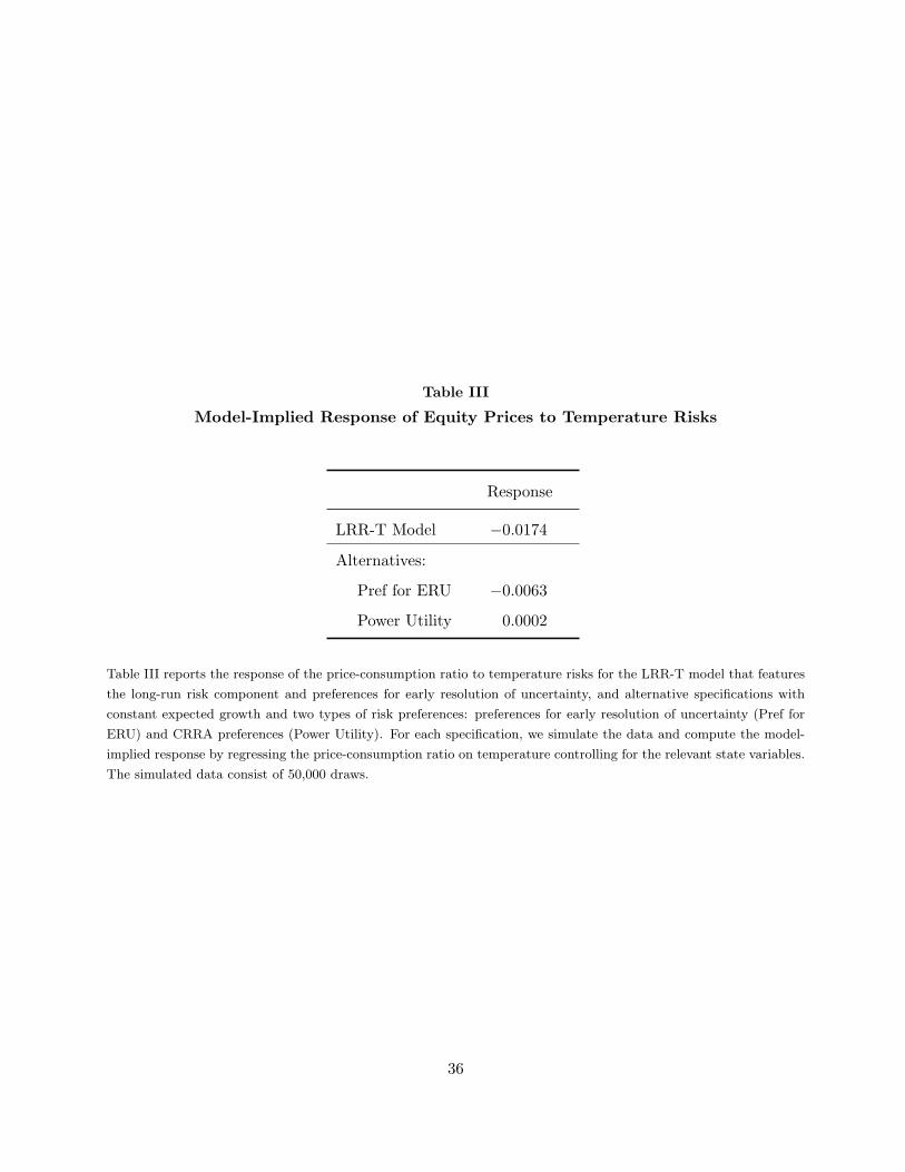
Table III

Model-Implied Response of Equity Prices to Temperature Risks

Response

LRR-T Model −0.0174

Alternatives:

Pref for ERU −0.0063

Power Utility 0.0002

Table III reports the response of the price-consumption ratio to temperature risks for the LRR-T model that features

the long-run risk component and preferences for early resolution of uncertainty, and alternative specifications with

constant expected growth and two types of risk preferences: preferences for early resolution of uncertainty (Pref for

ERU) and CRRA preferences (Power Utility). For each specification, we simulate the data and compute the model-

implied response by regressing the price-consumption ratio on temperature controlling for the relevant state variables.

The simulated data consist of 50,000 draws.

36

Table IV

Capital Market Implications

LRR-T Alternative Specifications

Model Pref for ERU Power Utility

SCC 103.6 39.01 0.01

Risk-Free Rate 0.91 2.11 10.08

Risk Premia 1.70 0.16 0.17

Discount Rates:

10yr Strip 1.51 2.28 10.33

100yr Strip 2.41 2.29 10.31

Table IV presents the social cost of carbon (SCC) and asset pricing implications of the LRR-T Model that features

the long-run risk component and preferences for early resolution of uncertainty, and alternative specifications with

constant expected growth and two types of risk preferences: preferences for early resolution of uncertainty (Pref for

ERU) and CRRA preferences (Power Utility). SCC is measured in 2012 dollars of world consumption per metric ton

of carbon. The risk-free rate and risk premia on consumption claim are averaged over the transitional path, discount

rates represent expected rates of returns on consumption strips with 10- and 100-year maturities. Returns and premia

are expressed in annualized percentage terms.

37

Table V

Long-Run Temperature Betas

Panel A: 25 BM/Size Sorted Portfolios

Small 2 3 4 Large

Growth −0.027 −0.016 0.014 0.009 0.024

2 −0.015 −0.012 −0.012 −0.002 −0.001

3 −0.014 −0.014 −0.015 −0.005 −0.016

4 −0.018 −0.024 −0.021 −0.027 −0.006

Value −0.038 −0.041 −0.055 −0.016 −0.010

Panel B: Industry Portfolios

High Heat-Exposed Low Heat-Exposed

MINE −0.014 MANU 0.006

OILG −0.024 WHOS −0.009

CNST −0.037 RETS 0.005

TRAN −0.023 SERV 0.014

UTIL −0.026 COMM 0.010

Table V shows long-run temperature betas of 25 book-to-market and size sorted portfolios (Panel A) and 10 industry

portfolios (Panel B) estimated by regressing portfolio excess returns on the five-year change in temperature controlling

for market and consumption growth risks. Industry classification of high and low heat-exposed sectors is according to

the National Institute for Occupational Safety and Health. The data are annual and cover the 1934-2014 period.

38

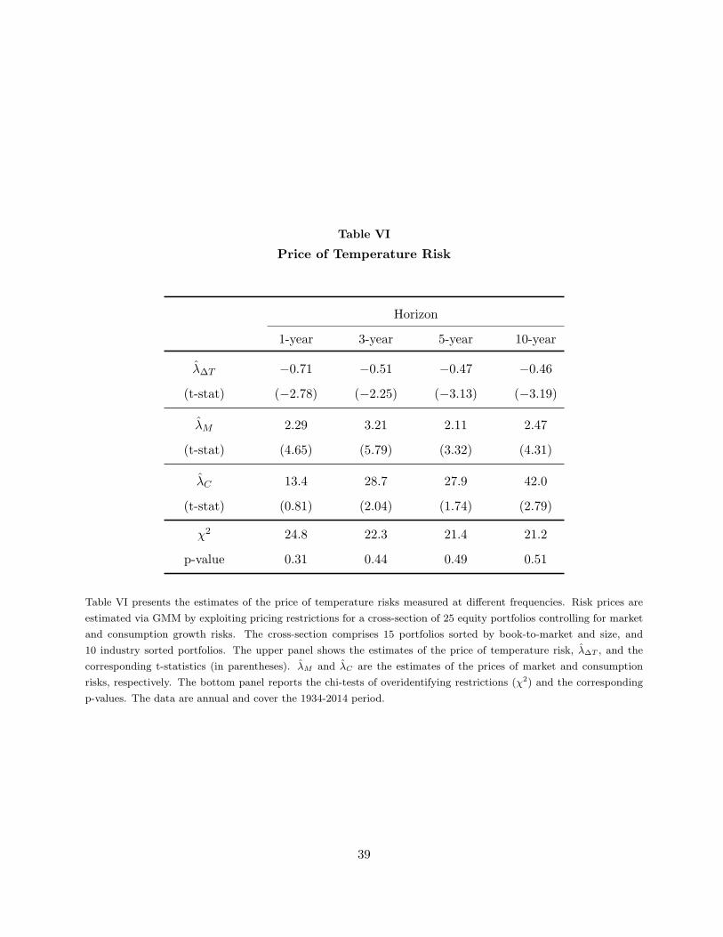
Table VI

Price of Temperature Risk

Horizon

1-year 3-year 5-year 10-year

λ∆T −0.71 −0.51 −0.47 −0.46

(t-stat) (−2.78) (−2.25) (−3.13) (−3.19)

λM 2.29 3.21 2.11 2.47

(t-stat) (4.65) (5.79) (3.32) (4.31)

λC 13.4 28.7 27.9 42.0

(t-stat) (0.81) (2.04) (1.74) (2.79)

χ2 24.8 22.3 21.4 21.2

p-value 0.31 0.44 0.49 0.51

Table VI presents the estimates of the price of temperature risks measured at different frequencies. Risk prices are

estimated via GMM by exploiting pricing restrictions for a cross-section of 25 equity portfolios controlling for market

and consumption growth risks. The cross-section comprises 15 portfolios sorted by book-to-market and size, and

10 industry sorted portfolios. The upper panel shows the estimates of the price of temperature risk, λ∆T , and the

corresponding t-statistics (in parentheses). λM and λC are the estimates of the prices of market and consumption

risks, respectively. The bottom panel reports the chi-tests of overidentifying restrictions (χ2) and the corresponding

p-values. The data are annual and cover the 1934-2014 period.

39

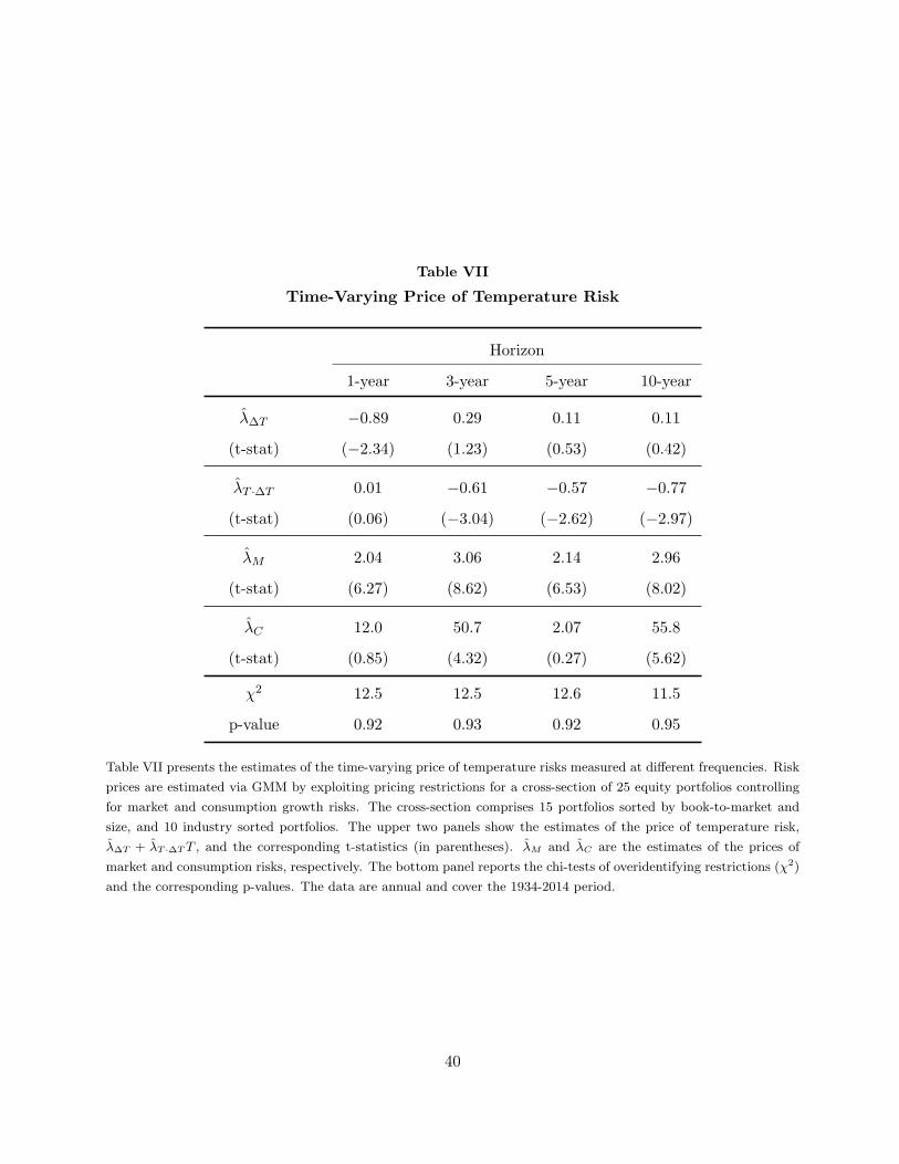
Table VII

Time-Varying Price of Temperature Risk

Horizon

1-year 3-year 5-year 10-year

λ∆T −0.89 0.29 0.11 0.11

(t-stat) (−2.34) (1.23) (0.53) (0.42)

λT ·∆T 0.01 −0.61 −0.57 −0.77

(t-stat) (0.06) (−3.04) (−2.62) (−2.97)

λM 2.04 3.06 2.14 2.96

(t-stat) (6.27) (8.62) (6.53) (8.02)

λC 12.0 50.7 2.07 55.8

(t-stat) (0.85) (4.32) (0.27) (5.62)

χ2 12.5 12.5 12.6 11.5

p-value 0.92 0.93 0.92 0.95

Table VII presents the estimates of the time-varying price of temperature risks measured at different frequencies. Risk

prices are estimated via GMM by exploiting pricing restrictions for a cross-section of 25 equity portfolios controlling

for market and consumption growth risks. The cross-section comprises 15 portfolios sorted by book-to-market and

size, and 10 industry sorted portfolios. The upper two panels show the estimates of the price of temperature risk,

λ∆T + λT ·∆TT , and the corresponding t-statistics (in parentheses). λM and λC are the estimates of the prices of

market and consumption risks, respectively. The bottom panel reports the chi-tests of overidentifying restrictions (χ2)

and the corresponding p-values. The data are annual and cover the 1934-2014 period.

40

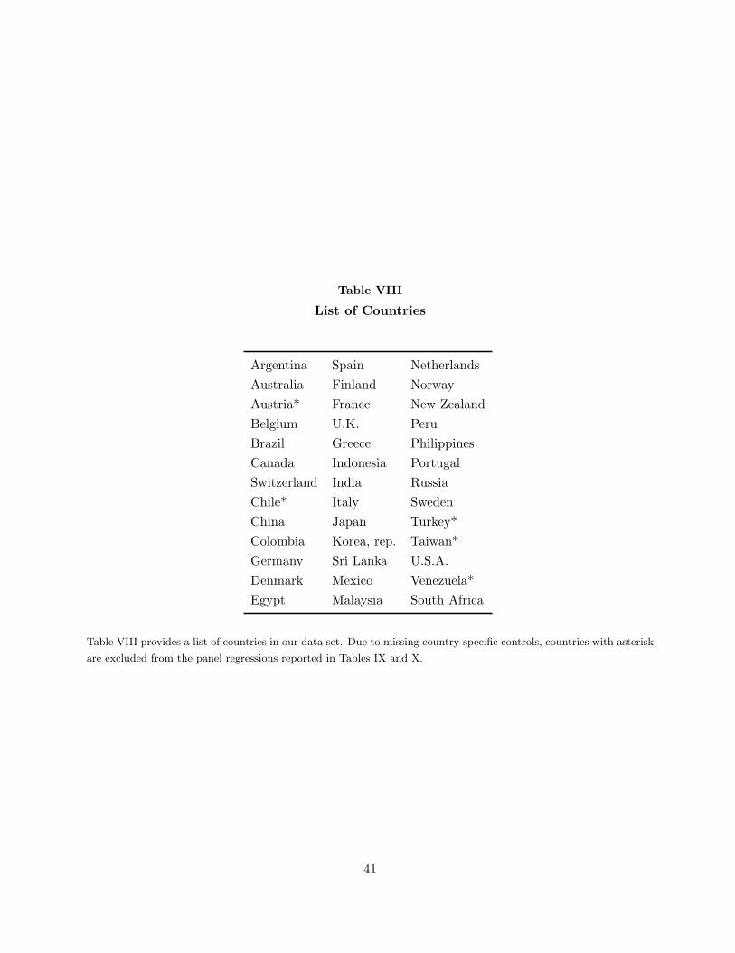
Table VIII

List of Countries

Argentina Spain Netherlands

Australia Finland Norway

Austria* France New Zealand

Belgium U.K. Peru

Brazil Greece Philippines

Canada Indonesia Portugal

Switzerland India Russia

Chile* Italy Sweden

China Japan Turkey*

Colombia Korea, rep. Taiwan*

Germany Sri Lanka U.S.A.

Denmark Mexico Venezuela*

Egypt Malaysia South Africa

Table VIII provides a list of countries in our data set. Due to missing country-specific controls, countries with asterisk

are excluded from the panel regressions reported in Tables IX and X.

41

Table IX

Elasticity of Equity Prices to Temperature Variations

Horizon Sample ϕK t-stat

1980−2000 −0.016 −1.51

K = 1yr 1980−2005 −0.043 −3.21

1980−2009 −0.076 −4.41

1980−2000 −0.040 −1.48

K = 3yr 1980−2005 −0.094 −3.40

1980−2009 −0.138 −5.59

1980−2000 0.058 1.79

K = 5yr 1980−2005 −0.023 −0.56

1980−2009 −0.105 −3.33

Table IX reports the response of equity prices to temperature risks estimated in the following panel regression:

vi,t = vi + ϕK TKi,t + α′

xXi,t + αvvi,t−1 + εi,t ,

where vi,t is the log of the price-dividend ratio of country i, vi is the country-specific fixed effect, TKi,t is a K-year

moving-average of local temperature, and Xi,t is a set of global and local controls. The set of controls includes two

common price-dividend ratio-based factors and country-specific inflation, unemployment, real interest rate, and gdp

growth. The parameters are estimated using the Arellano and Bond (1991)’s GMM estimator applied to the first-

differenced data. The table presents the estimates of the slope coefficient, ϕK , and the corresponding t-statistics based

on the White (1980)’s robust estimator of the variance-covariance matrix. The panel comprises 34 countries over the

1980-2009 period.

42

Table X

Equity Response to Long- and Short-Run Temperature Risks

Estimate t-stat

K = 3yr

ϕLR −0.138 −4.78

ϕSR −0.026 −1.00

K = 5yr

ϕLR −0.135 −3.37

ϕSR −0.028 −1.05

Table X reports the response of equity valuations to long- and short-run temperature risks estimated in the followingpanel regression:

vi,t = vi + ϕLR LRKi,t + ϕSR SRi,t + α′xXi,t + αvvi,t−1 + εi,t ,

where vi,t is the log of the price-dividend ratio of country i, vi is the country-specific fixed effect, LRKi,t proxies

for low-frequency temperature risks and is measured by the three- or five-year moving-average of local temperature,

SRi,t is annual temperature orthogonalized with respect to long-run fluctuations, and Xi,t is a set of global and local

controls. The set of controls includes two common price-dividend ratio-based factors and country-specific inflation,

unemployment, real interest rate, and gdp growth. The parameters are estimated using the Arellano and Bond (1991)’s

GMM estimator applied to the first-differenced data. The table presents the estimates of the slope coefficients, ϕLR

and ϕSR, and the corresponding t-statistics based on the White (1980)’s robust estimator of the variance-covariance

matrix. The panel comprises 34 countries over the 1980-2009 period.

43

Table XI

VAR Dynamics of Equity Prices and Temperature

T8i,t Ti,t vi,t

T8i,t−1 0.921 0.385 −0.093

[ 107.1 ] [ 7.06 ] [−2.29 ]

Ti,t−1 0.026 0.158 −0.017

[ 5.44 ] [ 5.19 ] [−0.73 ]

vi,t−1 0.014 0.076 0.520

[ 3.15 ] [ 2.65 ] [ 24.41 ]

R2 0.96 0.31 0.67

Table XI shows the estimates of the first-order panel VAR for equity prices and temperature. T8i,t denotes the eight-

year moving-average of local temperature, Ti,t is annual temperature series, and vi,t is the log of the price-dividend

ratio of country i. The exogenous variables included in the VAR comprise two price-dividend ratio factors that control

for common macro-economic risks and country-specific fixed effects. T-statistics are reported in brackets. The panel

consists of 39 countries over the 1970-2012 period.

44

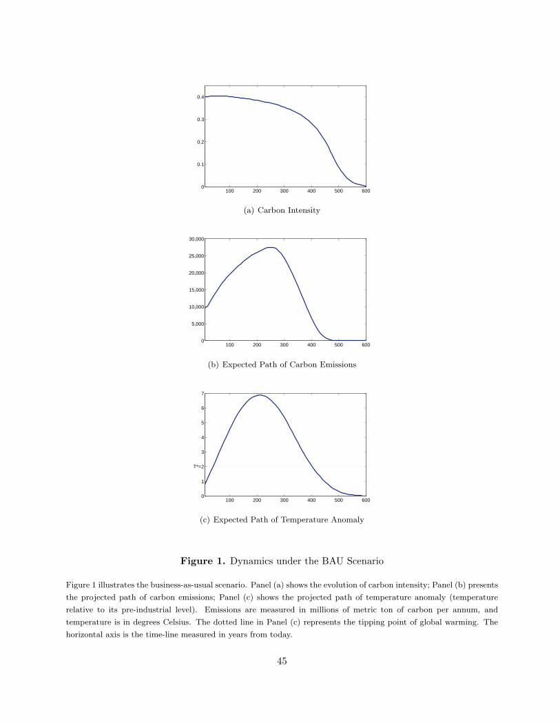
100 200 300 400 500 6000

0.1

0.2

0.3

0.4

(a) Carbon Intensity

100 200 300 400 500 6000

5,000

10,000

15,000

20,000

25,000

30,000

(b) Expected Path of Carbon Emissions

100 200 300 400 500 6000

1

2

3

4

5

6

7

T*=

(c) Expected Path of Temperature Anomaly

Figure 1. Dynamics under the BAU Scenario

Figure 1 illustrates the business-as-usual scenario. Panel (a) shows the evolution of carbon intensity; Panel (b) presents

the projected path of carbon emissions; Panel (c) shows the projected path of temperature anomaly (temperature

relative to its pre-industrial level). Emissions are measured in millions of metric ton of carbon per annum, and

temperature is in degrees Celsius. The dotted line in Panel (c) represents the tipping point of global warming. The

horizontal axis is the time-line measured in years from today.

45

100 200 300 400 500 6000

0.005

0.010

0.015

0.020

0.025

0.030

(a) Disaster Intensity

100 200 300 400 500 600−0.07

−0.06

−0.05

−0.04

−0.03

−0.02

−0.01

0

(b) Disaster Size

Figure 2. Global Warming Disasters under the BAU policy

Figure 2 shows the consequences of global warming in the business-as-usual case. Panel (a) plots the expected intensity

of climate change disasters per annum; Panel (b) shows the average annual size of disasters (−dt). The horizontal axis

is the time-line measured in years from today.

46

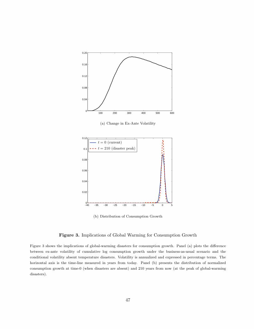
100 200 300 400 500 6000

0.04

0.08

0.12

0.16

0.20

(a) Change in Ex-Ante Volatility

−40 −35 −30 −25 −20 −15 −10 −5 0 50

0.02

0.04

0.06

0.08

0.1

0.12

t = 0 (current)

t = 210 (disaster peak)

(b) Distribution of Consumption Growth

Figure 3. Implications of Global Warming for Consumption Growth

Figure 3 shows the implications of global-warming disasters for consumption growth. Panel (a) plots the difference

between ex-ante volatility of cumulative log consumption growth under the business-as-usual scenario and the

conditional volatility absent temperature disasters. Volatility is annualized and expressed in percentage terms. The

horizontal axis is the time-line measured in years from today. Panel (b) presents the distribution of normalized

consumption growth at time-0 (when disasters are absent) and 210 years from now (at the peak of global-warming

disasters).

47

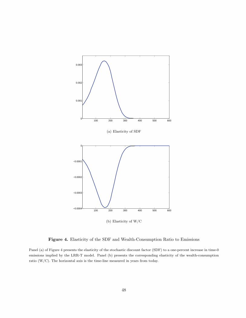
100 200 300 400 500 6000

0.001

0.002

0.003

(a) Elasticity of SDF

100 200 300 400 500 600−0.0004

−0.0003

−0.0002

−0.0001

0

(b) Elasticity of W/C

Figure 4. Elasticity of the SDF and Wealth-Consumption Ratio to Emissions

Panel (a) of Figure 4 presents the elasticity of the stochastic discount factor (SDF) to a one-percent increase in time-0

emissions implied by the LRR-T model. Panel (b) presents the corresponding elasticity of the wealth-consumption

ratio (W/C). The horizontal axis is the time-line measured in years from today.

48

100 200 300 400 500 600

−0.00006

−0.00004

−0.00002

0

0.00002

0.00004

0.00006

0.00008

Pref for ERUPower Utility

Figure 5. Sensitivity to Emissions

Figure 5 shows the elasticity of the wealth-consumption ratio to a one-percent increase in time-0 emissions for two

alternative specifications of preferences: preferences for early resolution of uncertainty (Pref for ERU) and CRRA

preferences (Power Utility). The horizontal axis is the time-line measured in years from today.

49

−0.05 −0.04 −0.03 −0.02 −0.01 0 0.01 0.02

0.08

0.1

0.12

0.14

0.16

0.18

Temperature Betas

Ave

rage

Exc

ess

Ret

urns

(a) Short-Run Temperature Betas

−0.05 −0.04 −0.03 −0.02 −0.01 0 0.01 0.02

0.08

0.1

0.12

0.14

0.16

0.18

Temperature Betas

Ave

rage

Exc

ess

Ret

urns

(b) Long-Run Temperature Betas

Figure 6. Temperature Betas

Figure 6 presents scatter plots of average excess returns and temperature betas of 25 book-to-market and size sorted

portfolios and 10 industry portfolios. Temperature betas are estimated by regressing portfolio excess returns on the

annual change in temperature (Panel A) and five-year change in temperature (Panel B) controlling for market and

consumption growth risks. Circles represent BM/size sorted portfolios; squares and asterisks correspond to high and

low heat-exposed industries, respectively, classified according to the National Institute for Occupational Safety and

Health. The data are annual and cover the 1934-2014 period.

50

1940 1950 1960 1970 1980 1990 2000 2010

0

0.004

0.008

0.012

Figure 7. Temperature Premium

Figure 7 plots the temperature risk premium of an equity portfolio with median size and book-to-market characteristics

based on the estimates reported in Table VII that correspond to the ten-year horizon.

51

0.4 0.6 0.8 1 1.2 1.40

1

2

3

4

5

6

7

Figure 8. Histogram of the Trend in Local Temperature

Figure 8 shows the histogram of the trend in local temperature measured by the change in average temperature over

the 2003-2012 period relative to the 1951-1980 average. The cross-sectional data comprise 39 countries; temperature

is measured in degrees Celsius.

52

1 2 3 4 5 6 7 8 9 10−0.05

−0.04

−0.03

−0.02

−0.01

0

0.01

0.02

(a) Response to Long-Run Shock

1 2 3 4 5 6 7 8 9 10−0.05

−0.04

−0.03

−0.02

−0.01

0

0.01

0.02

(b) Response to Short-Run Shock

Figure 9. Impulse Responses of Equity Prices to Long- and Short-Run Temperature Risks

Figure 9 presents impulse responses of the price-dividend ratio to long- and short-run temperature risks implied

by a first-order VAR. The estimated responses are represented by the solid lines, the shaded areas show the two

standard-error bands. Time-horizon on the horizontal axes is measured in years.

53