Learning and Shifts in Long-Run Productivity Growth

Rochelle M. Edge, Thomas Laubach, and John C. Williams∗

April 2, 2004

∗Board of Governors of the Federal Reserve System, rochelle.m.edge@frb.gov; Board of Governors of the

Federal Reserve System and OECD, thomas.laubach@oecd.org; and Federal Reserve Bank of San Francisco,

john.c.williams@sf.frb.org (corresponding author). We thank Michael Dotsey, John Fernald, Andreas Horn-

stein, Spencer Krane, Eric Leeper, Ed Nelson, Dave Reifschneider, Glenn Rudebusch, Tom Sargent, Argia

Sbordone, Stephanie Schmitt-Grohe, Michael Woodford, Raf Wouters, and participants at numerous pre-

sentations for comments on earlier versions of this paper. We also thank Kirk Moore for excellent research

assistance and Judith Goff for editorial assistance. The views expressed herein are those of the authors and

do not necessarily reflect those of the Board of Governors of the Federal Reserve System or their staff, the

management of the Federal Reserve Bank of San Francisco, or the OECD.

Abstract

Shifts in the long-run rate of productivity growth—such as those experienced by the

U.S. economy in the 1970s and 1990s—are difficult, in real time, to distinguish from

transitory fluctuations. In this paper, we analyze the evolution of forecasts of long-

run productivity growth during the 1970s and 1990s and examine in the context of

a dynamic general equilibrium model the consequences of gradual real-time learning

on the responses to shifts in the long-run productivity growth rate. We find that a

simple updating rule based on an estimated Kalman filter model using real-time data

describes economists’ long-run productivity growth forecasts during these periods ex-

tremely well. We then show that incorporating this process of learning has profound

implications for the effects of shifts in trend productivity growth and can dramatically

improve the model’s ability to generate responses that resemble historical experience.

If immediately recognized, an increase in the long-run growth rate causes long-term

interest rates to rise and produces a sharp decline in employment and investment, con-

trary to the experiences of the 1970s and 1990s. In contrast, with learning, a rise in

the long-run rate of productivity growth sets off a sustained boom in employment and

investment, with long-term interest rates rising only gradually. We find the character-

ization of learning to be crucial regardless of whether shifts in long-run productivity

growth owe to movements in TFP growth concentrated in the investment goods sector

or economy-wide TFP.

JEL Codes: E13, E32, D83, O40.

Keywords: DGE models, Kalman-filter, Real-time data, Learning, Productivity growth.

1 Introduction

An extensive literature has studied the effects of shocks to the level of productivity in

dynamic general equilibrium models. Surprisingly, despite the attention that has been

paid to documenting and understanding the 1970s productivity slowdown and the 1990s

acceleration, there has been relatively little formal analysis in the DGE framework on the

effects of a sustained shift in the rate of growth of productivity.1 A notable exception is

Campbell (1994), who found that in a real business cycle model a highly persistent reduction

in the productivity growth rate yielded the “perverse” response of a rise in employment

and output (see also the recent paper by Pakko, 2002).2 This result seems at odds with the

conventional wisdom that the productivity slowdown in the 1970s contributed to the woeful

macroeconomic performance of that decade and that the productivity acceleration of the

1990s was a central factor behind the remarkable performance in the late 1990s (Blinder

and Yellen 2002).

Research on the effects of a shift in long-run productivity growth has tended to assume

that agents immediately recognize the nature of such a shock and modify their expectations

and actions accordingly. In practice, sizable transitory fluctuations in productivity growth

obscure one’s view of the underlying trend growth rate. As a result, it takes years for even

professional economists to recognize that a shift has occurred, as evidenced by the debate

about the nature of the productivity slowdown during the 1970s and the acceleration in

the 1990s. In 1997, for example, Blinder (1997) placed the trend rate of labor productivity

growth at 1.1 percent, consistent with the average pace of productivity growth over the

preceding 23 years. Two years later, Gordon (1999) estimated trend productivity growth

to be 1.85 percent, a figure that he revised up to 2.25 percent in 2000 (in part due to

methodological changes in the national income accounts), and again to 2.5 percent in 20031Studies that provide early analysis of the causes of the productivity slowdown in the 1970s include

Denison (1979) and Norsworthy, Harper, and Kunze (1979), and the references cited therein. Jorgenson and

Stiroh (2000), Oliner and Sichel (2000), Basu, Fernald, and Shapiro (2001), and Gordon (2003) examine the

sources of the pickup in productivity growth in the 1990s.

2Other exceptions include include Brayton and Reifschneider (2001), who study the effects of a shift in

the long-run rate of productivity growth using the Federal Reserve Board’s large-scale macroeconometric

model, and Braun (1984) and Ball and Moffitt (2001), who study the effects on inflation in reduced-form

models.

1

(see Gordon 1999, 2000, 2003). As shown in this paper, this pattern of gradual learning

about shifts in long-run growth rate applies to both the 1970s and 1990s episodes.

In this paper we examine real-time estimates of trend productivity growth and compare

these to the predictions of a simple linear updating rule based on an estimated Kalman filter

model. We document that projections of long-run growth by economists and professional

forecasters adjust only gradually to this type of structural change: In the 1990s, for example,

the long-run productivity growth rate picked up significantly around the middle of the

decade, however, as noted above and documented below, the corresponding estimates by

economists and professional forecasters changed little until 1999 and shot up dramatically

in 2000.

We find that the real-time predictions of an estimated Kalman filter model track closely

the year-to-year movements in long-run expectations during both the 1970s and the 1990s.

Although economists use a wide variety of methods to estimate long-run trends, as discussed

by Lansing (2000), a simple linear updating rule approximates these methods extremely well.

Our model forecasts are constructed using a real-time dataset of labor productivity that we

collected. We show that the use of real-time data is crucial for understanding the historical

evolution of long-run expectations.3 Data revisions were especially pronounced during the

late 1990s, and they shaped the pattern of long-run expectations at the time.

We then examine the effects of learning regarding long-run productivity growth on the

responses to shifts in the trend growth rate in a standard optimization-based dynamic

general equilibrium model. Following on the results of Cummins and Violante (2002),

who emphasize the importance in the 1990s of shifts in the growth rate of productivity in

the investment-goods sector, we analyze shifts both to aggregate total factor productivity

(TFP) and to TFP in the investment goods sector alone. We calibrate the learning rate to be

consistent with the Kalman filter estimates and the survey evidence of long-run expectations.

We assume that agents in the model economy use the same Kalman filter updating formula

for long-run productivity growth that we found fits the survey data. One criticism of this

assumption is that agents may have greater information regarding their own idiosyncratic

economic prospects than the macroeconomic forecasters have about the aggregate rate of

productivity. Nonetheless, the expected future trajectory of any individual’s wages and rates3Our results are similar in spirit to those of Orphanides (2001) who examined the role of data revisions

in analyzing historical monetary policy.

2

of return depend on the aggregate level of wages and rates of return. Thus, in forecasting

the common component of wages and rates of return, agents face the same signal extraction

problem as macroeconomic forecasters.

We find that gradual recognition through learning has profoundly different implications

from immediate recognition for the economic effects of a shift in trend productivity growth.4

With gradual recognition through learning, we find that a permanent increase in the rate

of productivity growth boosts hours and investment at the onset of the shock and leads to

a sustained boom in employment and output growth. Under these learning assumptions,

agents initially believe that the shock is mainly transitory in nature and therefore has

minimal long-run implications for interest rates and the capital stock. As a result, the

stimulative effects of high productivity on employment and investment dominate and a

sustained boom ensues. In addition, with learning, long-term real bond rates rise only

gradually in response to a productivity acceleration, consistent with the evidence from

the late 1990s. In contrast, with immediate recognition, we obtain Campbell’s “perverse”

effects; specifically, a rise in long-run productivity growth elicits a rise in the natural rate

of interest. The resulting rise in real rates reduces the optimal ratio of capital to output,

implying that the existing stock of capital is too high. The productivity acceleration and

the implied capital overhang then generate a sharp decline in investment and employment.

The paper is organized as follows. Section 2 examines the evidence on real-time estimates

of long-run productivity growth during the 1970s and 1990s. Section 3 describes a simple

Kalman filter model and compares its real-time predictions of long-run productivity to evi-

dence from surveys and other documents. Section 4 describes both our optimization-based

dynamic general equilibrium model and the nonlinear model solution method. Section 5

analyzes the steady-state and dynamic implications of shifts in the growth rates of aggregate

and investment goods sector TFP. Section 6 concludes.

2 Real-time Estimates of Long-Run Productivity Growth

In this section, we document the real-time evolution of expectations of long-run productivity

growth during the 1970s and the 1990s, two periods during which the actual trend shifted4This paper focusses on the implications for the real side of the economy. In Edge, Laubach, and

Williams (2003), we further examine the implications of gradual recognition of a shift in long-run productivity

growth on prices and monetary policy.

3

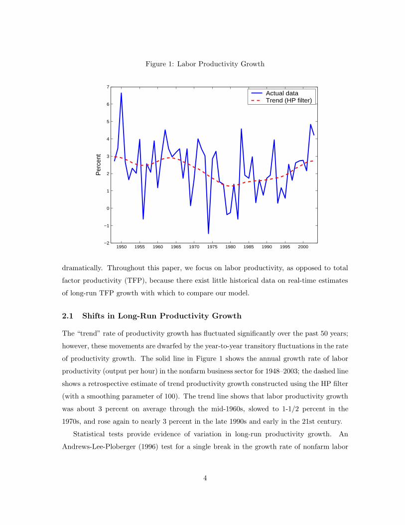
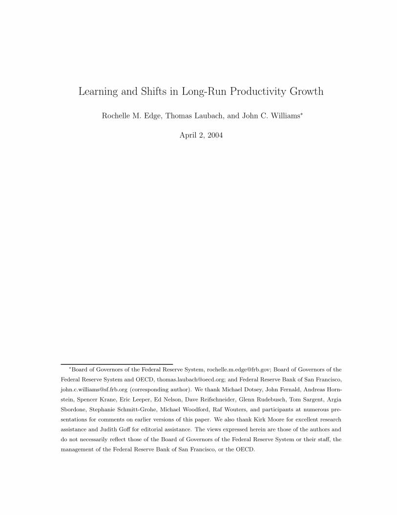
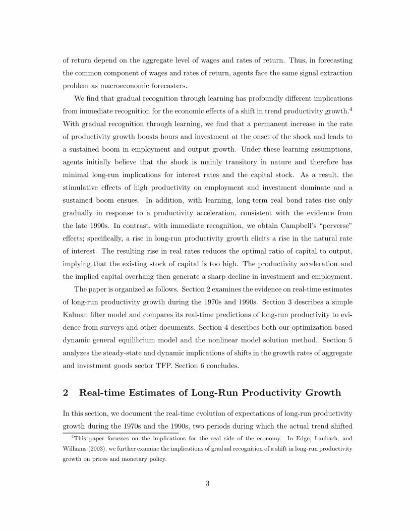
Figure 1: Labor Productivity Growth

1950 1955 1960 1965 1970 1975 1980 1985 1990 1995 2000−2

−1

0

1

2

3

4

5

6

7

Per

cent

Actual dataTrend (HP filter)

dramatically. Throughout this paper, we focus on labor productivity, as opposed to total

factor productivity (TFP), because there exist little historical data on real-time estimates

of long-run TFP growth with which to compare our model.

2.1 Shifts in Long-Run Productivity Growth

The “trend” rate of productivity growth has fluctuated significantly over the past 50 years;

however, these movements are dwarfed by the year-to-year transitory fluctuations in the rate

of productivity growth. The solid line in Figure 1 shows the annual growth rate of labor

productivity (output per hour) in the nonfarm business sector for 1948–2003; the dashed line

shows a retrospective estimate of trend productivity growth constructed using the HP filter

(with a smoothing parameter of 100). The trend line shows that labor productivity growth

was about 3 percent on average through the mid-1960s, slowed to 1-1/2 percent in the

1970s, and rose again to nearly 3 percent in the late 1990s and early in the 21st century.

Statistical tests provide evidence of variation in long-run productivity growth. An

Andrews-Lee-Ploberger (1996) test for a single break in the growth rate of nonfarm labor

4

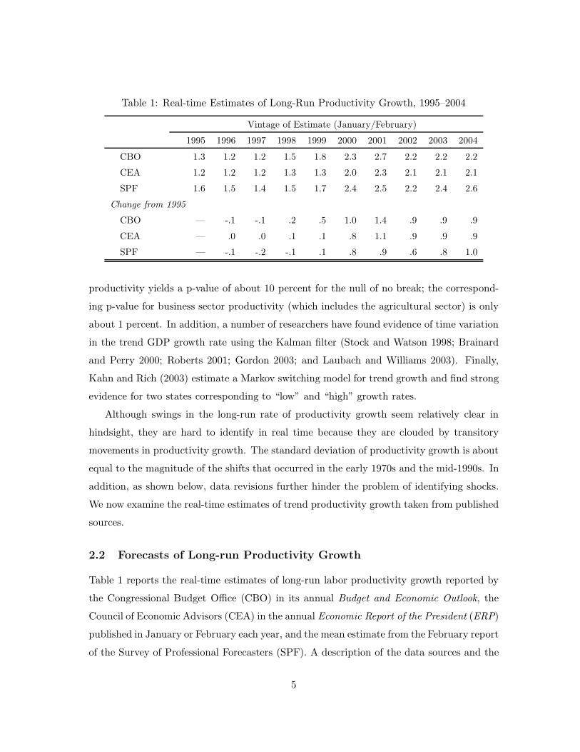
Table 1: Real-time Estimates of Long-Run Productivity Growth, 1995–2004

Vintage of Estimate (January/February)

1995 1996 1997 1998 1999 2000 2001 2002 2003 2004

CBO 1.3 1.2 1.2 1.5 1.8 2.3 2.7 2.2 2.2 2.2

CEA 1.2 1.2 1.2 1.3 1.3 2.0 2.3 2.1 2.1 2.1

SPF 1.6 1.5 1.4 1.5 1.7 2.4 2.5 2.2 2.4 2.6

Change from 1995

CBO — -.1 -.1 .2 .5 1.0 1.4 .9 .9 .9

CEA — .0 .0 .1 .1 .8 1.1 .9 .9 .9

SPF — -.1 -.2 -.1 .1 .8 .9 .6 .8 1.0

productivity yields a p-value of about 10 percent for the null of no break; the correspond-

ing p-value for business sector productivity (which includes the agricultural sector) is only

about 1 percent. In addition, a number of researchers have found evidence of time variation

in the trend GDP growth rate using the Kalman filter (Stock and Watson 1998; Brainard

and Perry 2000; Roberts 2001; Gordon 2003; and Laubach and Williams 2003). Finally,

Kahn and Rich (2003) estimate a Markov switching model for trend growth and find strong

evidence for two states corresponding to “low” and “high” growth rates.

Although swings in the long-run rate of productivity growth seem relatively clear in

hindsight, they are hard to identify in real time because they are clouded by transitory

movements in productivity growth. The standard deviation of productivity growth is about

equal to the magnitude of the shifts that occurred in the early 1970s and the mid-1990s. In

addition, as shown below, data revisions further hinder the problem of identifying shocks.

We now examine the real-time estimates of trend productivity growth taken from published

sources.

2.2 Forecasts of Long-run Productivity Growth

Table 1 reports the real-time estimates of long-run labor productivity growth reported by

the Congressional Budget Office (CBO) in its annual Budget and Economic Outlook, the

Council of Economic Advisors (CEA) in the annual Economic Report of the President (ERP)

published in January or February each year, and the mean estimate from the February report

of the Survey of Professional Forecasters (SPF). A description of the data sources and the

5

data series themselves are provided in the Appendix.5 The three series follow the same

pattern over this period. The differences in levels across the surveys may in part reflect

differences in concepts of labor productivity.6

Real-time estimates of long-run productivity growth adjusted only gradually to the

shift in underlying trend productivity growth during the 1990s. They dipped a bit in 1997,

and edged up in each of the next two years. Then, in 2000, they shot up, increasing by

0.5 percentage point (CBO) and 0.7 percentage point (CEA and SPF), after which they fell

following the 2001 recession. Compared to real-time estimates in 1995, the 2004 vintage

real-time estimates were up about 1 percentage point.

Hard data on real-time estimates of long-run productivity growth during the 1970s

are more difficult to come by; still, the available evidence indicates that economists only

gradually recognized the occurrence of the slowdown and only after five years or so fully

appreciated its magnitude. The CEA is the single source that approaches that of a consistent

time series. Table 2 reports real-time estimates of trend productivity growth from the ERP

for those years between 1970 and 1980 that such estimates were reported or could be directly

inferred from the text of the Report and supporting documents.

During the 1970s, the CEA revised down its forecasts of trend productivity growth in a

series of steps. In early 1970, its estimate of trend productivity growth in the entire economy

was 2.8 percent; in 1974, it revised the estimate down 0.4 percentage point; in 1977 the

estimate was revised down another 0.3 percentage point and then a further 0.6 percentage

point in 1979. The revisions in 1977 and 1979 were accompanied by detailed discussions in

the ERP outlining the CEA’s reassessments of long-run productivity and output trends.7

5As noted in the Appendix, only the CEA provides a reasonably consistent time series of medium-run

productivity projections that starts before the early 1990s. Explicit estimates from the CBO first appear in

the mid-1990s, and the SPF first started asking a question on long-run productivity growth in 1992.

6The projections reported by the CBO and CEA during this period explicitly refer to output per hour

in the nonfarm business sector, while the SPF survey simply refers to productivity growth. Productivity

growth can differ according to the measure used; for example, output per hour in the overall business sector

averaged 0.2 percentage points higher than that in the nonfarm business sector during 1973-1995 (according

to data available in early 1996), which is about the difference between the SPF and CBO estimates of

long-run productivity growth in 1996.

7See also Clark (1978), a staff member at the CEA at the time, who provides a detailed analysis of

the evidence for and causes of the productivity slowdown. By comparison, Perry (1977) remained very

optimistic about productivity’s trend growth rate in 1977. It was not until the late 1970s that a consensus

6

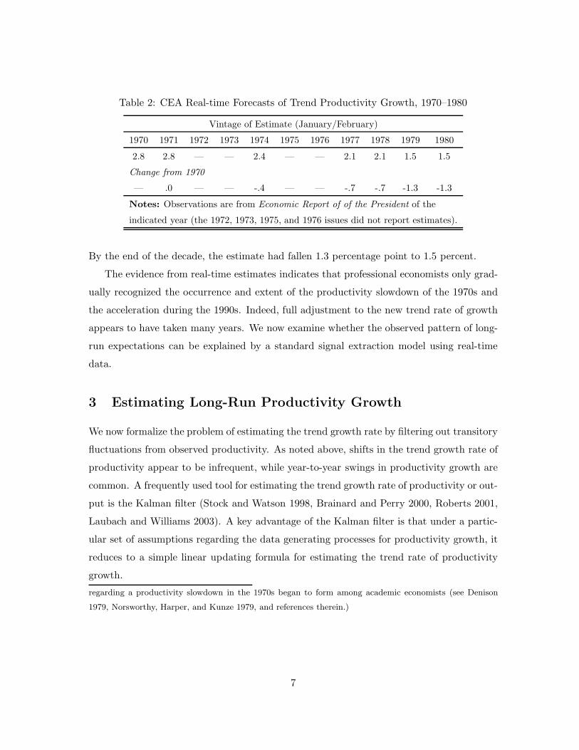
Table 2: CEA Real-time Forecasts of Trend Productivity Growth, 1970–1980

Vintage of Estimate (January/February)

1970 1971 1972 1973 1974 1975 1976 1977 1978 1979 1980

2.8 2.8 — — 2.4 — — 2.1 2.1 1.5 1.5

Change from 1970

— .0 — — -.4 — — -.7 -.7 -1.3 -1.3

Notes: Observations are from Economic Report of of the President of the

indicated year (the 1972, 1973, 1975, and 1976 issues did not report estimates).

By the end of the decade, the estimate had fallen 1.3 percentage point to 1.5 percent.

The evidence from real-time estimates indicates that professional economists only grad-

ually recognized the occurrence and extent of the productivity slowdown of the 1970s and

the acceleration during the 1990s. Indeed, full adjustment to the new trend rate of growth

appears to have taken many years. We now examine whether the observed pattern of long-

run expectations can be explained by a standard signal extraction model using real-time

data.

3 Estimating Long-Run Productivity Growth

We now formalize the problem of estimating the trend growth rate by filtering out transitory

fluctuations from observed productivity. As noted above, shifts in the trend growth rate of

productivity appear to be infrequent, while year-to-year swings in productivity growth are

common. A frequently used tool for estimating the trend growth rate of productivity or out-

put is the Kalman filter (Stock and Watson 1998, Brainard and Perry 2000, Roberts 2001,

Laubach and Williams 2003). A key advantage of the Kalman filter is that under a partic-

ular set of assumptions regarding the data generating processes for productivity growth, it

reduces to a simple linear updating formula for estimating the trend rate of productivity

growth.

regarding a productivity slowdown in the 1970s began to form among academic economists (see Denison

1979, Norsworthy, Harper, and Kunze 1979, and references therein.)

7

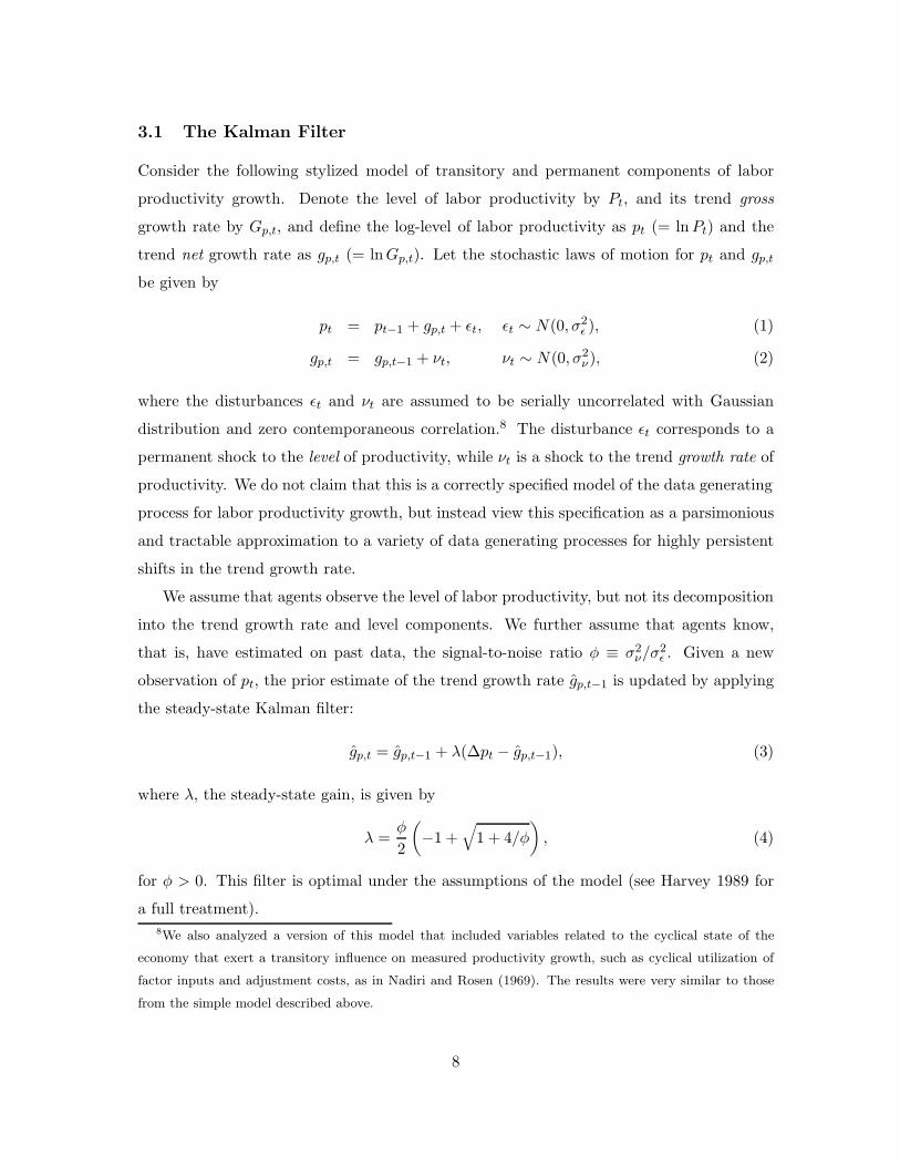
3.1 The Kalman Filter

Consider the following stylized model of transitory and permanent components of labor

productivity growth. Denote the level of labor productivity by Pt, and its trend gross

growth rate by Gp,t, and define the log-level of labor productivity as pt (= ln Pt) and the

trend net growth rate as gp,t (= ln Gp,t). Let the stochastic laws of motion for pt and gp,t

be given by

pt = pt−1 + gp,t + εt, εt ∼ N(0, σ2ε ), (1)

gp,t = gp,t−1 + νt, νt ∼ N(0, σ2ν), (2)

where the disturbances εt and νt are assumed to be serially uncorrelated with Gaussian

distribution and zero contemporaneous correlation.8 The disturbance εt corresponds to a

permanent shock to the level of productivity, while νt is a shock to the trend growth rate of

productivity. We do not claim that this is a correctly specified model of the data generating

process for labor productivity growth, but instead view this specification as a parsimonious

and tractable approximation to a variety of data generating processes for highly persistent

shifts in the trend growth rate.

We assume that agents observe the level of labor productivity, but not its decomposition

into the trend growth rate and level components. We further assume that agents know,

that is, have estimated on past data, the signal-to-noise ratio φ ≡ σ2ν/σ

2ε . Given a new

observation of pt, the prior estimate of the trend growth rate gp,t−1 is updated by applying

the steady-state Kalman filter:

gp,t = gp,t−1 + λ(∆pt − gp,t−1), (3)

where λ, the steady-state gain, is given by

λ =φ

2

(−1 +

√1 + 4/φ

), (4)

for φ > 0. This filter is optimal under the assumptions of the model (see Harvey 1989 for

a full treatment).8We also analyzed a version of this model that included variables related to the cyclical state of the

economy that exert a transitory influence on measured productivity growth, such as cyclical utilization of

factor inputs and adjustment costs, as in Nadiri and Rosen (1969). The results were very similar to those

from the simple model described above.

8

The key parameter for the Kalman filter is the gain λ that translates surprise movements

in the level of technology into perceived movements in the trend growth rate. Stock and

Watson (1998) estimate a quarterly model of GDP growth similar to that described above

with data through 1995, and their estimate implies a value of λ of 0.03 (per quarter).

Estimates by Roberts (2001) and Laubach and Williams (2003) that are based on data

through the end of the 1990s imply somewhat higher values for the gain.9 In each case, the

confidence bands around these estimates of the gain are very wide; for example, Laubach

and Williams (2003) find that the 90 percent confidence interval for their estimate of λ

includes zero.

Based on the Stock and Watson (1998) estimate, for our model of annual data, we take

0.115 as our benchmark value of λ. Given the uncertainty regarding estimates of λ, we also

consider two alternative values of λ: a lower value of 0.08 and a higher value of 0.22, where

the latter is equal to the value reported by Roberts (2001).

3.2 Real-time Kalman Filter Estimates

To compute real-time Kalman filter estimates, we first construct a set of real-time historical

annual data series of labor productivity, where each vintage of data corresponds to the data

available to economists at the end of January, about the time when estimates from the

CBO, CEA, and the SPF are reported. Throughout, the data source for a vintage is the

ERP, which is published near the beginning of the year.10

As we show in detail below, the use of real-time data is crucial for understanding the

evolution of historical long-run forecasts of productivity growth, especially during the late9Note that all of these estimates are based on final, revised data, and therefore they ignore real-time

measurement error noise that should damp the response of estimates of trend growth to unrevised data on

productivity. As a result, these estimates of the gain are likely biased upwards relative to the optimal gain.

The Kalman filter can be extended to include measurement error, which would yield a more complicated

updating rule. We leave that for future research.

10Fourth-quarter data for the preceding year is not yet published in early January. Therefore, we construct

a proxy for the fourth-quarter rate of productivity growth equal to the rate of productivity growth over the

preceding three quarters. We then compute the annual growth rate using the published data for the first

three quarters and our proxy for fourth-quarter growth. As a check on our method, we constructed alter-

native estimates using the real-time estimate of fourth-quarter productivity from the January or February

Greenbook prepared by the staff of the Board of Governors for years that data is publicly available (through

1999). The resulting Kalman filter estimates were nearly identical to those reported in the paper.

9

Table 3: Real-time Productivity Growth Data

Data Vintage (January)

Year 1995 1996 1997 1998 1999 2000 2001 2002 2003 2004

1990 0.5 0.5 0.5 0.5 0.5 1.2 1.2 1.2 1.2 1.3

1991 1.5 0.6 0.7 0.7 0.7 1.6 1.2 1.2 1.2 1.3

1992 2.7 3.2 3.2 3.2 3.1 4.1 3.7 3.7 3.7 3.6

1993 1.5 0.2 0.2 0.1 0.1 0.1 0.5 0.5 0.5 0.5

1994 2.2 0.5 0.5 0.4 0.5 1.3 1.3 1.3 1.3 1.3

1995 1.1 0.2 0.2 0.6 1.0 1.0 1.0 1.0 0.6

1996 0.7 1.3 2.5 2.7 2.5 2.5 2.5 2.5

1997 1.9 1.4 1.9 1.8 2.0 2.0 1.6

1998 2.1 2.8 2.7 2.6 2.6 2.6

1999 2.8 2.9 2.4 2.4 2.7

2000 4.4 3.3 2.9 2.8

2001 1.7 1.1 2.2

2002 4.9 4.8

2003 4.2

1990s when data revisions were substantial.11 Table 3 reports the published rates of growth

of labor productivity in the nonfarm business sector for each vintage of data from 1995

through 2004 (as described above). Published figures for productivity growth, especially

for 1995 and 1996, changed dramatically as the data were revised. According to the 1997

vintage, productivity growth actually slowed in 1995 and 1996 relative to its average over

the previous 20 years. The 1999 vintage exhibits upward revisions to productivity growth

for 1995 and 1996, along with a strong figure for 1998. A portion of the upward revision

in the 2000 vintage of productivity data reflects changes in the way that gross domestic

output is measured in the national income accounts. According to analysis in the 2000

ERP, methodological changes boosted measured real GDP growth by 0.4 percentage point

in 1987–1994, and by 0.2 percentage point in 1995–1998.

We next compute annual real-time Kalman filter estimates of trend productivity growth

using our real-time data sets and the estimated value of the Kalman gain. For each vintage11Gordon (2000) also emphasizes the importance of data revisions and changes in methodology in account-

ing for revisions to his estimates of trend productivity growth.

10

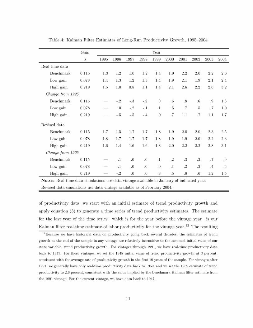
Table 4: Kalman Filter Estimates of Long-Run Productivity Growth, 1995–2004

Gain Year

λ 1995 1996 1997 1998 1999 2000 2001 2002 2003 2004

Real-time data

Benchmark 0.115 1.3 1.2 1.0 1.2 1.4 1.9 2.2 2.0 2.2 2.6

Low gain 0.078 1.4 1.3 1.2 1.3 1.4 1.9 2.1 1.9 2.1 2.4

High gain 0.219 1.5 1.0 0.8 1.1 1.4 2.1 2.6 2.2 2.6 3.2

Change from 1995

Benchmark 0.115 — -.2 -.3 -.2 .0 .6 .8 .6 .9 1.3

Low gain 0.078 — .0 -.2 -.1 .1 .5 .7 .5 .7 1.0

High gain 0.219 — -.5 -.5 -.4 .0 .7 1.1 .7 1.1 1.7

Revised data

Benchmark 0.115 1.7 1.5 1.7 1.7 1.8 1.9 2.0 2.0 2.3 2.5

Low gain 0.078 1.8 1.7 1.7 1.7 1.8 1.9 1.9 2.0 2.2 2.3

High gain 0.219 1.6 1.4 1.6 1.6 1.8 2.0 2.2 2.2 2.8 3.1

Change from 1995

Benchmark 0.115 — -.1 .0 .0 .1 .2 .3 .3 .7 .9

Low gain 0.078 — -.1 .0 .0 .0 .1 .2 .2 .4 .6

High gain 0.219 — -.2 .0 .0 .3 .5 .6 .6 1.2 1.5

Notes: Real-time data simulations use data vintage available in January of indicated year.

Revised data simulations use data vintage available as of February 2004.

of productivity data, we start with an initial estimate of trend productivity growth and

apply equation (3) to generate a time series of trend productivity estimates. The estimate

for the last year of the time series—which is for the year before the vintage year—is our

Kalman filter real-time estimate of labor productivity for the vintage year.12 The resulting12Because we have historical data on productivity going back several decades, the estimates of trend

growth at the end of the sample in any vintage are relatively insensitive to the assumed initial value of our

state variable, trend productivity growth. For vintages through 1991, we have real-time productivity data

back to 1947. For these vintages, we set the 1948 initial value of trend productivity growth at 3 percent,

consistent with the average rate of productivity growth in the first 10 years of the sample. For vintages after

1991, we generally have only real-time productivity data back to 1959, and we set the 1959 estimate of trend

productivity to 2.6 percent, consistent with the value implied by the benchmark Kalman filter estimate from

the 1991 vintage. For the current vintage, we have data back to 1947.

11

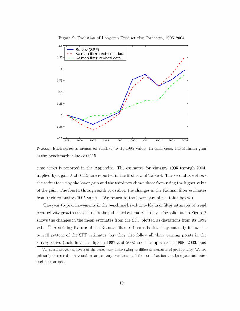
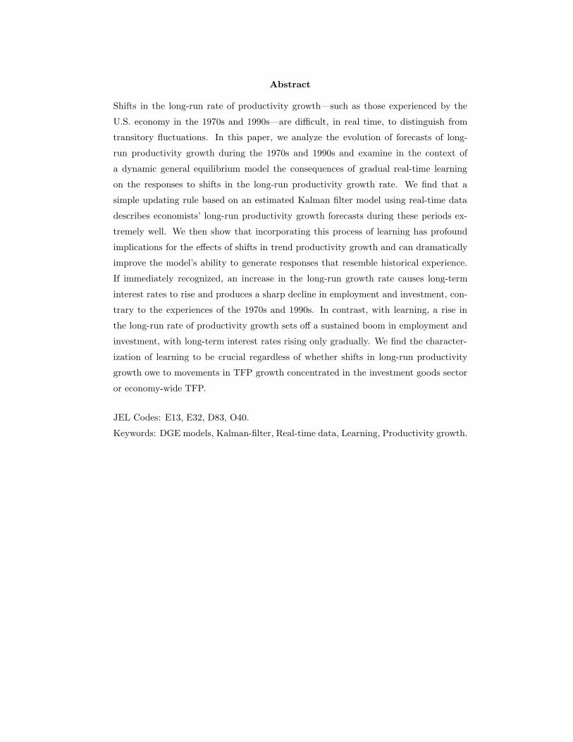
Figure 2: Evolution of Long-run Productivity Forecasts, 1996–2004

1995 1996 1997 1998 1999 2000 2001 2002 2003 2004−0.5

−0.25

0

0.25

0.5

0.75

1

1.25

1.5

Survey (SPF)Kalman filter: real−time dataKalman filter: revised data

Notes: Each series is measured relative to its 1995 value. In each case, the Kalman gain

is the benchmark value of 0.115.

time series is reported in the Appendix. The estimates for vintages 1995 through 2004,

implied by a gain λ of 0.115, are reported in the first row of Table 4. The second row shows

the estimates using the lower gain and the third row shows those from using the higher value

of the gain. The fourth through sixth rows show the changes in the Kalman filter estimates

from their respective 1995 values. (We return to the lower part of the table below.)

The year-to-year movements in the benchmark real-time Kalman filter estimates of trend

productivity growth track those in the published estimates closely. The solid line in Figure 2

shows the changes in the mean estimates from the SPF plotted as deviations from its 1995

value.13 A striking feature of the Kalman filter estimates is that they not only follow the

overall pattern of the SPF estimates, but they also follow all three turning points in the

survey series (including the dips in 1997 and 2002 and the upturns in 1998, 2003, and13As noted above, the levels of the series may differ owing to different measures of productivity. We are

primarily interested in how such measures vary over time, and the normalization to a base year facilitates

such comparisons.

12

2004). Although not shown in the figure, the Kalman filter estimates also track well the

estimates from the CBO and the CEA reported in Table 1. In addition, the benchmark

Kalman filter estimates line up well with the real-time estimates reported by Blinder (1997)

and Gordon (1999, 2000, 2003) in the introduction of the paper. Note that since only past

data on productivity growth are used in constructing the Kalman filter estimates, the close

correspondence between these estimates and the published real-time estimates cannot be

attributed to some auxiliary assumptions or data.

The Kalman filter estimates that use the higher value of the gain are more volatile

than those in the SPF and those from the CBO, and the CEA. As seen in Table 4, the

Kalman filter estimate using the high value of the gain is 1.7 percentage points above its

1995 level in 2004, while the published estimates rose only about 1 percentage point over the

same period. The Kalman filter estimates based on a lower value of the gain of 0.078, also

reported in Table 4, are smoother than the benchmark estimate, and track the changes in

the SPF over the 1996-2004 period about as well as the benchmark Kalman filter estimates.

Indeed, a value of λ of about of 0.10 yields Kalman filter estimates that best fit the changes

in the SPF over this sample.

The close fit of the Kalman filter estimates of trend productivity growth to the pub-

lished estimates in the recent episode depends critically on the use of real-time data. The

lower portion of Table 4 reports Kalman filter estimates using revised data from February

2004. Unlike the real-time published estimates, the Kalman filter estimates using revised

data show a steady rise during the second half of the 1990s, reflecting the rapid pace of

productivity gains during that period. Comparing the two Kalman filter estimates in Fig-

ure 2 illustrates the critical importance of using real-time data in empirically analyzing the

evolution of expectations.

Economists did not substantially revise upwards their views on trend growth earlier be-

cause the real-time productivity data through 1998 showed no evidence of any acceleration.

As shown in Table 3, according to the data available in early 1997, productivity growth had

actually slowed relative to its previous trend. This dip in productivity growth explains the

drop in the real-time Kalman filter estimates and is consistent with the fall in the CBO and

SPF estimates that year.

Upward revisions to past data and the robust pace of productivity growth in 1998

drive up the Kalman filter estimate in 1999, again consistent with the pattern seen in

13

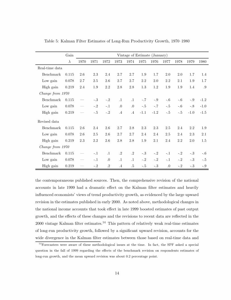
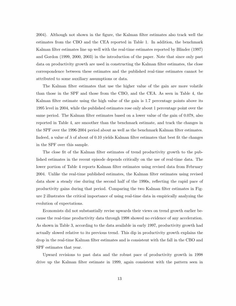
Table 5: Kalman Filter Estimates of Long-Run Productivity Growth, 1970–1980

Gain Vintage of Estimate (January)

λ 1970 1971 1972 1973 1974 1975 1976 1977 1978 1979 1980

Real-time data

Benchmark 0.115 2.6 2.3 2.4 2.7 2.7 1.9 1.7 2.0 2.0 1.7 1.4

Low gain 0.078 2.7 2.5 2.6 2.7 2.7 2.2 2.0 2.2 2.1 1.9 1.7

High gain 0.219 2.4 1.9 2.2 2.8 2.8 1.3 1.2 1.9 1.9 1.4 .9

Change from 1970

Benchmark 0.115 — -.3 -.2 .1 .1 -.7 -.9 -.6 -.6 -.9 -1.2

Low gain 0.078 — -.2 -.1 .0 .0 -.5 -.7 -.5 -.6 -.8 -1.0

High gain 0.219 — -.5 -.2 .4 .4 -1.1 -1.2 -.5 -.5 -1.0 -1.5

Revised data

Benchmark 0.115 2.6 2.4 2.6 2.7 2.8 2.3 2.3 2.5 2.4 2.2 1.9

Low gain 0.078 2.6 2.5 2.6 2.7 2.7 2.4 2.4 2.5 2.4 2.3 2.1

High gain 0.219 2.3 2.2 2.6 2.8 2.8 1.9 2.1 2.4 2.2 2.0 1.5

Change from 1970

Benchmark 0.115 — -.1 .1 .2 .2 -.3 -.2 -.1 -.2 -.3 -.6

Low gain 0.078 — -.1 .0 .1 .1 -.2 -.2 -.1 -.2 -.3 -.5

High gain 0.219 — -.2 .2 .4 .5 -.5 -.3 .0 -.2 -.3 -.9

the contemporaneous published sources. Then, the comprehensive revision of the national

accounts in late 1999 had a dramatic effect on the Kalman filter estimates and heavily

influenced economists’ views of trend productivity growth, as evidenced by the large upward

revision in the estimates published in early 2000. As noted above, methodological changes in

the national income accounts that took effect in late 1999 boosted estimates of past output

growth, and the effects of these changes and the revisions to recent data are reflected in the

2000 vintage Kalman filter estimates.14 This pattern of relatively weak real-time estimates

of long-run productivity growth, followed by a significant upward revision, accounts for the

wide divergence in the Kalman filter estimates between those based on real-time data and14Forecasters were aware of these methodological issues at the time. In fact, the SPF asked a special

question in the fall of 1999 regarding the effects of the benchmark revision on respondents estimates of

long-run growth, and the mean upward revision was about 0.2 percentage point.

14

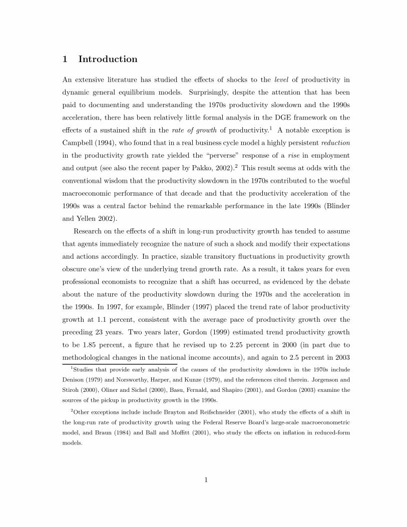
Figure 3: Evolution of Long-run Productivity Expectations in the 1970s

1970 1971 1972 1973 1974 1975 1976 1977 1978 1979 1980−1.5

−1.25

−1

−0.75

−0.5

−0.25

0

0.25

CEAKalman filter: real−time dataKalman filter: revised data

Notes: All series are relative to the respective 1970 value. The squares indicate the available

observations. The Kalman filter estimates are based on an annual gain of 0.115.

those based on revised data.

Kalman filter estimates from the 1970s track the implicit estimates of trend productivity

growth from the CEA during the late 1970s reasonably well. The solid line in Figure 3 shows

the CEA estimates (the squares indicate years for which we have readings from the ERP).

The dashed line shows the benchmark Kalman filter estimates. The estimates for the three

values of the gain are reported in the upper part of Table 5. As before, the Kalman filter

estimates with the high value of the gain are excessively volatile relative to the real-time

published estimates.

Overall, the benchmark Kalman filter estimates do a remarkable job of matching the

real-time estimates of long-run productivity growth during the periods of the productivity

slowdown in the 1970s and following the acceleration in the 1990s. We now turn to the

implications of gradual recognition on the dynamic responses of the economy to a shift in

the trend rate of productivity growth.

15

4 The Model Economy

We illustrate the effects of the gradual recognition of a shift in productivity growth using

a standard two-sector neoclassical growth model with endogenous labor supply. In this

section, we describe a standard real business cycle model and the solution method. In

the following section, we analyze the effects of permanent shocks to the growth rate of

productivity.

4.1 Production Technology and Preferences

Let Ct and It denote the output of the consumption and investment goods sectors in period t.

The technologies to produce consumption and investment are assumed to be identical except

for a scale factor reflecting the different levels of TFP in the two sectors. Specifically, the

production of consumption and investment goods are given by:

Ct = A1−αt Kα

c,tL1−αc,t (5)

It = (ZtAt)1−α Kα

i,tL1−αi,t (6)

where Kj,t and Lj,t denote the quantities of capital and labor employed in each sector j, At

represents the aggregate technology process that affects both sectors equally, and Zt is the

technology process that is specific to the investment-goods producing sector.

The aggregate capital accumulation technology is given by:

Kt+1 = (1 − δ)Kt + It, (7)

where δ is the rate of physical depreciation. We assume that capital is freely mobile across

the two sectors, where the sum of the two capital stocks used in production is restricted

not to exceed the aggregate capital stock; specifically, Kc,t + Ki,t ≤ Kt.

The representative household’s welfare at time 0 is given by:

E0

∞∑t=0

βtUt, (8)

where β is the household’s rate of time preference and Ut denotes the momentary utility in

period t. Utility is given by:

Ut =

ln CtHt

+ ζ ln(1 − Lt

Ht

)for γ = 1,

11−γ

[CtHt

(1 − Lt

Ht

)ζ]1−γ

otherwise,(9)

16

where Ht denotes the size of the household, Lt represents total labor input from the house-

hold, γ is the inverse of the household’s intertemporal elasticity of consumption, and ζ is

a parameter that governs the household’s elasticity of labor supply. We assume that la-

bor is freely mobile across the two sectors, where the sum of the labor inputs in the two

sectors cannot exceed the aggregate labor input that period: Lc,t + Li,t ≤ Lt, which itself

may not exceed the aggregate time endowment. Since we normalize the time endowment of

each member of the household to unity, the aggregate time endowment is equal to Ht. We

assume that the population grows at a constant gross rate Gh, specifically, Ht+1 = GhHt.

4.2 The Decentralized Competitive Equilibrium

Given the assumptions regarding technology and preferences and the absence of distortions

in the model economy, the decentralized competitive equilibrium is equivalent to the solu-

tion of the social planning problem that maximizes the welfare of the representative agent.

We start by characterizing the solution to the social planner’s problem with complete in-

formation about all shocks. In the next section, we turn to the solution where expectations

are based on an estimate of long-run productivity growth computed using a version of the

Kalman filter.

The planner’s problem in period t is to maximize household welfare (equation 8) subject

to the consumption and investment sector production functions (equations 5 and 6), the

accumulation equation (equation 7), and the two factor market constraints. The resulting

first-order conditions to the social planner’s problem are given by:

Ct

Kc,t=

ItZ−(1−α)t

Ki,t, (10)

Ct

Lc,t=

ItZ−(1−α)t

Li,t, (11)

U ′c,tZ

−(1−α)t = βEtU

′c,t+1

(α

Ct+1

Kc,t+1+ (1 − δ)Z−(1−α)

t+1

), (12)

ζLc,t

Ht= (1 − α)

(1 − Lt

Ht

), (13)

where U ′c,t denotes the marginal utility of consumption. Equations (10) and (11) equate

the marginal product of capital and labor across the two sectors. Because the production

functions are identical up to a multiplicative term, the two sectors employ labor and capital

in the same proportions in both sectors. Equation (12) is the standard intertemporal Euler

17

equation, augmented to include changes in the relative productivity of the investment goods

sector. Equation (13) is the within period condition for the choice of labor input. The

marginal rate of transformation between investment goods and consumption, that is, the

relative “price” of investment goods, is given by Z−(1−α)t .

It is useful to construct a real output measure consistent with the current use of chain-

weighted aggregation in the U.S. national income accounts. Correspondingly, we define real

aggregate output, Yt, as the Divisia index sum of real consumption and real investment:

∆ ln Yt =Ct

Y Nt

∆ lnCt +INt

Y Nt

∆ ln It,

where INt

(≡ ItZ

−(1−α)t

)represents nominal investment and Y N

t

(≡ Ct + IN

t

)denotes

nominal output. Again for comparison to the data, we construct a synthetic real 10-year

bond rate, Rb, determined according to an approximation of the expectations theory of the

term structure:

Rbt =

111

(Rt + Et10Rb

t+1

), (14)

where Rt = Z(1−α)t Et

(α Ct+1

Kc,t+1+ (1 − δ)Z−(1−α)

t+1

)is the ex ante real return to capital.

4.3 The Deterministic Steady State

To characterize the deterministic balanced growth steady state of the model, we assume that

A and Z increase at constant gross growth rates Ga and Gz , respectively. The steady-state

growth rates of consumption, investment, and output are then given by:

Gc = GhGaGαz , (15)

Gi = GhGaGz, (16)

Gy = Gscc G1−sc

i , . (17)

where Gx denotes the steady-state gross growth rate of variable X, and sc denotes the

steady-state ratio of labor employed producing consumption goods. Along the balanced

growth path, labor input increases at a gross rate Gh, and the aggregate capital stock

increases at the same rate as investment. In the steady-state, hours per person is constant.

Thus, the steady-state rate of growth of labor productivity equals the ratio of the steady-

state growth rate of output to that of population. Nominal investment and nominal output

increase at the same rate as real consumption.

18

To solve and simulate the model, it is useful to work with normalized variables, which are

denoted by lower case letters. In particular, the following normalizations yield stationary

variables along the balanced growth path: l = LH , c = C

HAZα , i = IHAZ , k = K

HAZ .

The first-order condition for the consumption-saving choice (equation 12) yields the

following steady-state relationship between the gross real rate of return on capital, R, and

the growth rate of per capita consumption:

R = β−1(

Gc

Gh

)γ

. (18)

The steady-state ratio of the normalized capital stock to normalized output, denoted by κ,

is given by:

κ =αG

−(1−α)z

R − (1 − δ)G−(1−α)z

(19)

The steady-state share of labor used to produce consumption goods is given by:

sc = 1 − (Gi − 1 + δ)κ. (20)

The labor-leisure choice yields the steady-state per capita labor supply, denoted by l,

l =1 − α

ζsc + 1 − α. (21)

4.4 Calibration

For the simulations, we calibrate the model to annual data using standard parameter values

taken from the literature. In particular, we set α = 0.36, β = 0.98, γ = 1, ζ = 3, and

δ = 0.10. We calibrate the steady-state growth rates from long-run post-war averages: Gz =

1.014, Ga = 1.014 and Gh = 1.014. Together these imply annual steady-state per capita

growth rates of 1.9 percent for consumption, 2.8 percent for investment, and 2.2 percent for

chain-weighted output (and labor productivity).

4.5 Solution Method

The model simulations consider permanent shocks to the trend growth rates of technology.

Unlike shocks to the level of technology typically studied in the literature, these shocks

imply permanent changes in the levels of normalized variables. For example, the steady-

state consumption share and labor input both depend on the steady-state growth rates Ga

and Gz. Therefore, log-linear approximations around a particular steady-state may provide

19

relatively poor approximations to the dynamic response to growth shocks. For this reason,

we use nonlinear methods to compute the dynamic responses to the shocks. Following

Judd (1992), we use higher-order polynomial approximations to the decision rules describing

the behavior of the economy.15

We use orthogonal collocation, which is an application of Galerkin methods described

in Fletcher (1984), to compute the approximate decision rules. In particular, the decision

rules for labor input and consumption are approximated by fifth-order polynomial functions

of the three state variables: the normalized capital stock, the trend growth rate of aggre-

gate technology, and the trend growth rate of investment-goods technology. A Chebyshev

polynomial basis is used to represent the decision rules; tensor products of the states are

used in the polynomial representations. A nonlinear equation solver is used to find the

coefficients of the decision rules that satisfy the stochastic first-order equations at a fixed

set of points in the three states, where the points are the roots of the Chebyshev polyno-

mial basis. Expectations in the first-order equations are approximated using an eight-point

Gauss-Hermite quadrature rule. This method is extremely efficient and accurate.16 Using

these approximate decision rules and the law of motion of the economy, we compute impulse

responses to shocks to the technology processes, with each impulse response starting at the

balanced-growth steady state.

5 Effects of Shifts in the Trend Growth Rate

In this section, we consider simulations of permanent shocks to the growth rate of technol-

ogy. We consider two alterative sources for the shift in productivity growth. In one, the

change affects both the consumption and investment goods sectors equally, roughly consis-

tent with the evidence from the productivity slowdown in the 1970s. In the second, the15We compared the simulation results using the nonlinear method to those obtained using a log-

linearization of the system. The log-linear simulations were generally reasonably close to those using the

nonlinear method; the largest deviation occurs in the response of labor input.

16It takes 20 seconds on a 1.2Mhz Pentium III computer to solve for the fifth-order polynomial decision

rules of this model. One metric for approximation error used by Judd (1992) is the maximum absolute error

in the first-order equations, normalized to be in terms of consumption units, computed over a wide range of

points for the state variables. For the model in this paper, the maximum absolute error is less than 0.001

percent.

20

shift occurs only in the investment goods sector, consistent with the evidence of Cummins

and Violante (2002) regarding the productivity acceleration in the 1990s. We first examine

the long-run implications of such shocks and then analyze the dynamic path via which the

model economy arrives at the new long-run equilibrium.

5.1 Steady-state Effects

Consider first the steady-state effects of a permanent increase in the growth rate of the

aggregate technology process, Ga. From the steady-state conditions we see that a percent-

age point increase in the growth rate of aggregate technology implies an increase of the

same magnitude in the steady-state growth rates of per capita consumption, investment,

and output (equation 15 and 17). The implied faster rate of decline in marginal utility

implies a higher real return on capital (equation 18), as consumers demand a higher return

on savings to forgo consumption today. The higher real return in turn implies a lower

steady-state normalized capital-to-output ratio (equation 19). The consumption-to-output

ratio (equation 20) may rise or fall depending on two opposing effects: Faster growth ne-

cessitates greater investment to hold the normalized capital-to-output ratio constant; but,

the higher rate of return implies a lower optimal capital-to-output ratio. It is not possible

to sign a priori the net effect on the consumption-to-output ratio. In addition, it is not

possible to sign the steady-state effect on labor supply (equation 21), since labor supply is

a decreasing function of the consumption-to-output ratio. For our calibration, the former

effect dominates, and the steady-state consumption-to-output ratio falls in response to an

increase in the rate of growth of aggregate TFP. As a result, labor supply rises slightly with

an increase in Ga.

Now consider the effects of a permanent increase in the growth rate of the investment-

specific technology process Gz. A percentage point increase in the growth rate of investment-

sector TFP has a smaller effect on consumption growth than a change in aggregate TFP

growth of the same magnitude (equation 15), since the former increases consumption growth

only through the capital-deepening channel. We therefore consider a slightly larger increase

in the growth rate of Gz; specifically, one which yields a percentage point increase in the

growth rate of consumption and hence an increase in the real interest rate equal to that

implied by our aggregate TFP growth-rate shock (equation 18). Despite generating the

same-sized increase in real interest rates, the investment sector productivity acceleration—

21

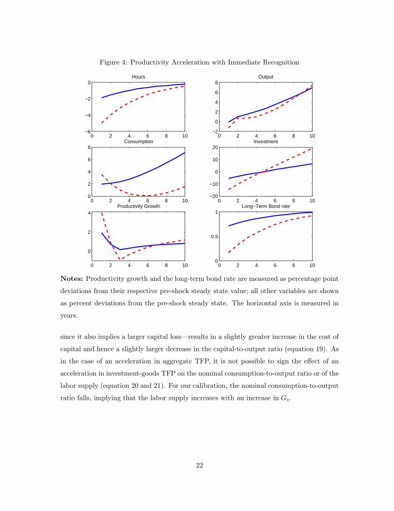
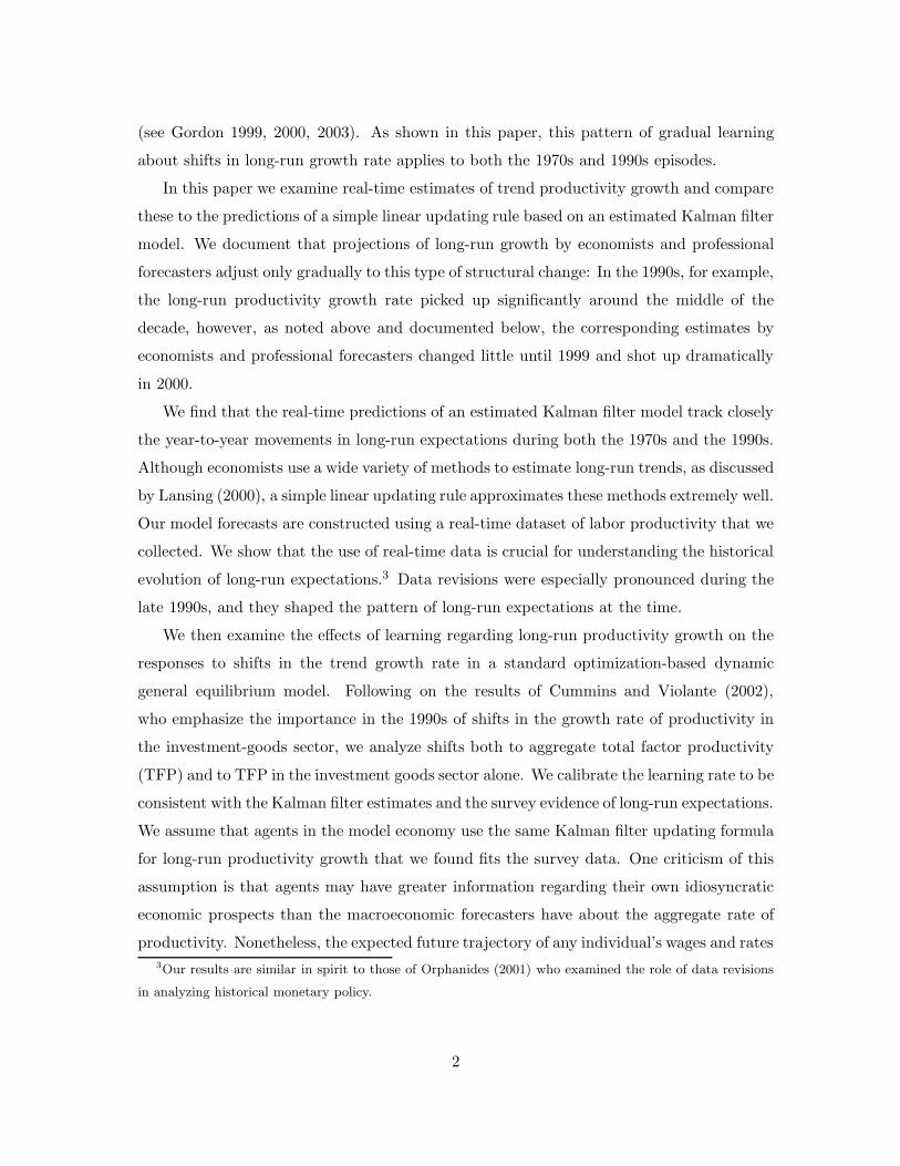
Figure 4: Productivity Acceleration with Immediate Recognition

0 2 4 6 8 10−6

−4

−2

0Hours

0 2 4 6 8 10−2

0

2

4

6

8Output

0 2 4 6 8 100

2

4

6

8Consumption

0 2 4 6 8 10−20

−10

0

10

20Investment

0 2 4 6 8 10

0

2

4Productivity Growth

0 2 4 6 8 100

0.5

1Long−Term Bond rate

Notes: Productivity growth and the long-term bond rate are measured as percentage point

deviations from their respective pre-shock steady state value; all other variables are shown

as percent deviations from the pre-shock steady state. The horizontal axis is measured in

years.

since it also implies a larger capital loss—results in a slightly greater increase in the cost of

capital and hence a slightly larger decrease in the capital-to-output ratio (equation 19). As

in the case of an acceleration in aggregate TFP, it is not possible to sign the effect of an

acceleration in investment-goods TFP on the nominal consumption-to-output ratio or of the

labor supply (equation 20 and 21). For our calibration, the nominal consumption-to-output

ratio falls, implying that the labor supply increases with an increase in Gz.

22

5.2 Dynamic Responses to an Observed Productivity Acceleration

We now consider the effects of an unanticipated increase in the rate of growth of aggregate

TFP that is immediately observed, where the shock is scaled to yield a one percentage point

long-run increase in the growth rates of consumption. The solid lines in Figure 4 show the

results of this experiment.

At the onset of an increase in the rate of trend aggregate TFP growth, the existing

capital-to-output ratio exceeds its new steady-state level, since, as just discussed, the higher

rate of long-run growth implies a higher long-run rate of return, as seen by the response

of the long-term bond rate. The equilibrium response to the resulting capital overhang is

a sharp decline in investment, which generates the required liquidation of capital. Con-

sumption increases immediately following the shock, offsetting the decline in investment

and leaving output about unchanged, and hours decline.17 These negative responses of

investment and hours following a positive shock to aggregate TFP growth are consistent

with the “perverse” pattern noted by Campbell (1994).18 After the initial phase during

which capital stocks are run down, investment growth picks up again and attains its new

balanced growth path. In the long run, consumption, investment, and output increase one

percentage point faster than before the shock to aggregate TFP growth.

Qualitatively, the responses to an unanticipated permanent increase in the growth rate

of investment-specific TFP—shown by the dashed lines in Figure 4—are similar to those of

an upward shift in the growth rate of economy-wide TFP. The shock is scaled to yield the

same one percentage point increase in the growth rate of consumption and nominal output

as the previous experiment. Real investment initially falls following the shock as do hours

and real output.

5.3 Dynamic Responses with Learning

We now modify the model to allow for imperfect information about whether the shock to

productivity growth is transitory or permanent. As noted in the introduction, we assume17In this model, hours rise in response to a productivity acceleration only if labor supply is highly inelastic

and households have a very high rate of intertemporal substitution.

18Campbell (1994) simulated a highly persistent negative shock to the rate of productivity growth, while

we simulate a permanent positive one. The distinction between a highly persistent shock and a permanent

one is not important, as the two experiments yield qualitatively similar results.

23

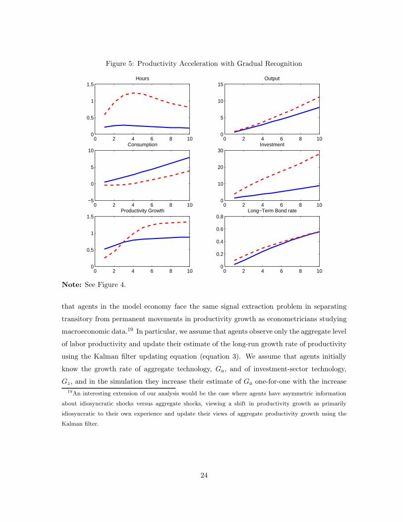
Figure 5: Productivity Acceleration with Gradual Recognition

0 2 4 6 8 100

0.5

1

1.5Hours

0 2 4 6 8 100

5

10

15Output

0 2 4 6 8 10−5

0

5

10Consumption

0 2 4 6 8 100

10

20

30Investment

0 2 4 6 8 100

0.5

1

1.5Productivity Growth

0 2 4 6 8 100

0.2

0.4

0.6

0.8Long−Term Bond rate

Note: See Figure 4.

that agents in the model economy face the same signal extraction problem in separating

transitory from permanent movements in productivity growth as econometricians studying

macroeconomic data.19 In particular, we assume that agents observe only the aggregate level

of labor productivity and update their estimate of the long-run growth rate of productivity

using the Kalman filter updating equation (equation 3). We assume that agents initially

know the growth rate of aggregate technology, Ga, and of investment-sector technology,

Gz, and in the simulation they increase their estimate of Ga one-for-one with the increase19An interesting extension of our analysis would be the case where agents have asymmetric information

about idiosyncratic shocks versus aggregate shocks, viewing a shift in productivity growth as primarily

idiosyncratic to their own experience and update their views of aggregate productivity growth using the

Kalman filter.

24

in the estimate of trend labor productivity generated by Kalman filter updating.20 Note

that for this experiment the updating of trend productivity growth is applied only to the

perceived trend growth rate of aggregate TFP; we assume that the perceived trend growth

rate of investment-specific TFP is not affected. We set the gain λ for updating estimates of

trend labor productivity growth equal to 0.115, consistent with the evidence from Kalman

filter estimation and from economists’ real-time estimates of trend productivity growth, as

discussed above. (Later, we examine the sensitivity of our results to the choice of the gain.)

In an economy where agents filter incoming information to estimate the trend productiv-

ity growth rate, hours, output, and investment all rise in response to a permanent increase

in aggregate TFP growth, and, as a result, the economy experiences a prolonged boom.

The solid line in Figure 5 reports the results from the same experiment of a permanent

increase in the growth rate of aggregate TFP as before but with gradual recognition of the

source of the shock. In the first few years after the onset of the shock, agents believe that

the trend growth rate has risen only very modestly and attribute most of the higher level

of productivity to a sequence of positive shocks to the level of productivity (εt shocks in

terms of our notation in equations 1 and 2). In this model, such level shocks boost hours,

output, and investment, with only relatively small effects on the real interest rate.21 Only

when the perceived long-run rate of productivity growth rises do rates on long-term bonds

rise significantly as well.22

20We also have conducted these experiments assuming that agents directly update their expectations of

trend TFP growth based on observations of TFP instead of indirectly through their observations of labor

productivity growth. The results are very similar to those reported here.

21Our model predicts hours to increase following a positive permanent shock to the level of technology and

is in this respect consistent with the empirical responses reported by Altig, Christiano, Eichenbaum, and

Linde (2002) and Christiano, Eichenbaum, and Vigfusson (2003a, 2003b). In contrast, Basu, Fernald, and

Kimball (1998), Galı (1999), and Francis and Ramey (2001) find that hours initially decline in response to

a positive permanent shock to the level of TFP, although this decline is generally only transitory such that

a rise in employment eventually transpires. Thus, even in a model that generates an hours response similar

to the those found by these authors, a string of positive shocks still leads to a lagged boom in employment.

Thus, our conclusions as to the importance of agents initially mistaking an acceleration in TFP growth as a

sequence of TFP level shocks do not rely on sign of the impact response of hours to a permanent shock to

the level of productivity.

22Brayton and Reifschneider (2001) examine shifts in long-run productivity using the Federal Reserve’s

large-scale macroeconomic model, and also find that an increase in the long-run rate of productivity growth

generates a sustained boom in employment and investment. Importantly, in their model simulations, interest

25

The effects of an acceleration in productivity in the investment-goods sector alone is

shown by the dashed lines of Figure 5. For this experiment, we assume that agents under-

stand that the shock is specific to the investment-goods sector but do not know whether

the increase in productivity growth is transitory or permanent. We use the same gain λ

as before but adjust the updating formula to reflect the fact that an increase in Gz has a

proportionally smaller effect on aggregate labor productivity growth than a similar-sized

increase in Ga. In the calibrated model, Gz must increase by 0.018 to raise the steady-state

growth of output by 0.01. Thus, we multiply an increase in estimated trend aggregate labor

productivity growth by a factor of 1.8 to compute the implied increase in the perceived

value of Gz .

As before, the productivity acceleration generates a prolonged rise in hours and a mono-

tonic increase in the rate of labor productivity growth and the long-term bond rate. One

interesting distinction between the two shocks is that the dynamics of the investment-goods

sector productivity acceleration are more drawn out.

Learning has important implications for the response of long-term bond rates to shifts

in trend productivity. If an increase in the long-run rate of productivity growth were

immediately recognized, the model predicts a significant rise in real long-term yields within

a few years of the onset of the shock. With learning, real-long terms yields rise very

gradually during the decade following the shock. The evidence from SPF expectations of

future real interest rates during the late 1990s provides some support for the model with

learning. SPF long-run expectations of real interest rates changed relatively little during

the late 1990s, before declining during the recession of 2001. Similarly, yields on inflation-

indexed securities (TIIS) increased gradually during the late 1990s.23 Of course, other

factors, including fiscal policy and the state of the business cycle, influenced expectations of

real interest rates during this period, making a sharp comparison of the model predictions

and the data difficult.

In summary, the model with learning predicts that a productivity acceleration leads to

a prolonged boom in hours and a steady increase in the rate of output and productivity

growth. The implied rise in long-term real rates occurs very gradually. These results are

rates rise only gradually in response to the faster rate of growth.

23TIIS securities were first issued in early 1997. See Bomfim (2001) for a discussion of the use of TIIS

yields in measuring real rate expectations.

26

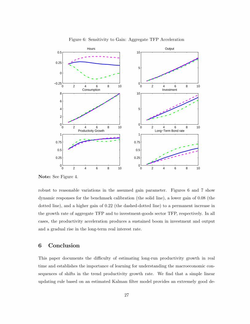
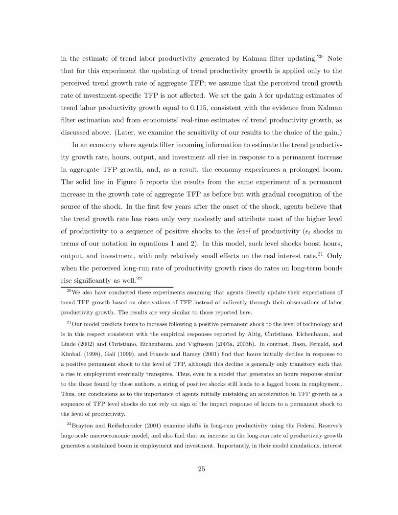
Figure 6: Sensitivity to Gain: Aggregate TFP Acceleration

0 2 4 6 8 10−0.25

0

0.25

0.5Hours

0 2 4 6 8 100

5

10Output

0 2 4 6 8 100

2

4

6

8Consumption

0 2 4 6 8 100

5

10Investment

0 2 4 6 8 100

0.25

0.5

0.75

1Productivity Growth

0 2 4 6 8 100

0.25

0.5

0.75

1Long−Term Bond rate

Note: See Figure 4.

robust to reasonable variations in the assumed gain parameter. Figures 6 and 7 show

dynamic responses for the benchmark calibration (the solid line), a lower gain of 0.08 (the

dotted line), and a higher gain of 0.22 (the dashed-dotted line) to a permanent increase in

the growth rate of aggregate TFP and to investment-goods sector TFP, respectively. In all

cases, the productivity acceleration produces a sustained boom in investment and output

and a gradual rise in the long-term real interest rate.

6 Conclusion

This paper documents the difficulty of estimating long-run productivity growth in real

time and establishes the importance of learning for understanding the macroeconomic con-

sequences of shifts in the trend productivity growth rate. We find that a simple linear

updating rule based on an estimated Kalman filter model provides an extremely good de-

27

Figure 7: Sensitivity to Gain: Investment-Goods Sector TFP Acceleration

0 2 4 6 8 100

0.5

1

1.5Hours

0 2 4 6 8 100

5

10

15Output

0 2 4 6 8 10−2

0

2

4Consumption

0 2 4 6 8 100

10

20

30

40Investment

0 2 4 6 8 100

0.5

1

1.5Productivity Growth

0 2 4 6 8 100

0.2

0.4

0.6

0.8Long−Term Bond rate

Note: See Figure 4.

scription of the evolution of economists’ real-time estimates of long-run productivity growth

over both the 1970s and 1990s. We then show that incorporating the gradual recognition

of shifts in trend growth rate has considerable implications for the dynamic responses to

such shocks: If immediately recognized, an increase in the long-run productivity growth

rate—in what is markedly at odds with historical experience—causes long-term interest

rates to rise and generates a sharp decline in employment and investment. By contrast, an

identical model that differs only in that it allows for the gradual recognition of shifts in the

trend growth rate of TFP can, following a sustained rise in the rate of productivity growth,

generate positive and prolonged responses for hours and investment, and a more gradual

increase in long-term interest rates. Moreover, for our preferred calibration of the pace of

learning about productivity growth rate shifts—which equals the learning rate consistent

with published real time estimates of long-run productivity growth—an increase (decrease)

28

in the long-run growth rate of productivity generates a sustained employment and invest-

ment boom (slump). This prediction represents a dramatic improvement in our model’s

ability to generate responses to long-run productivity growth rate shifts that resemble the

experiences of the 1970s and 1990s.

References

[1] Altig, David, Lawrence J. Christiano, Martin Eichenbaum, and Jesper Linde. “Tech-

nology Shocks and Aggregate Fluctuations.” Federal Reserve Bank of Chicago,

manuscript, June 2002.

[2] Andrews, Donald, Inpyo Lee, and Werner Ploberger. “Optimal Changepoint Tests for

Normal Linear Regression.” Journal of Econometrics 70(1), January 1996, 9–38.

[3] Ball, Laurence and Robert Moffitt. “Productivity Growth and the Phillips Curve.”

Johns Hopkins University, manuscript, June 2001.

[4] Basu, Susanto, John Fernald, and Miles S. Kimball. “Are Technology Improvements

Contractionary?” Federal Reserve Board, International Finance Discussion Papers 625,

September 1998.

[5] Basu, Susanto, John Fernald, and Matthew D. Shapiro. “Productivity Growth in the

1990s: Technology, Utilization, or Adjustment?” Federal Reserve Bank of Chicago

Working Paper 2001-4, June 2001.

[6] Blinder, Alan S. “The Speed Limit: Fact and Fancy in the Growth Debate.” The

American Prospect 8(34) September-October 1997.

[7] Blinder, Alan S., and Janet L. Yellen. “The Fabulous Decade: Macreconomic Lessons

from the 1990s.” In: Alan B. Krueger and Robert M. Solow (eds.) The Roaring 1990s:

Can Full Employment Be Sustained? New York: Russel Sage Foundation, 2002.

[8] Bomfim, Antulio N. “Measuring Equilibrium Real Interest Rates: What Can We Learn

from Yields on Indexed Bonds?” Federal Reserve Board, FEDS working paper 2001-53,

November 2001.

29

[9] Brainard, William C., and George L. Perry. “Making Policy in a Changing World.” In:

George L. Perry and James Tobin (eds.) Economic Events, Ideas, and Policies : The

1960’s and After Washington, DC: Brookings Institution Press, 2000, 43–82.

[10] Braun, Steven. “Productivity and the NIIRU (and Other Phillips Curve Issues).” Board

of Governors of the Federal Reserve System, Working Paper 34, 1984.

[11] Brayton, Flint and David Reifschneider. “U.S. Macroeconomic Performance Since the

Mid-1990s: The FRB/US View,” Manuscript, Federal Reserve Board, April 2001.

[12] Campbell, John Y. “Inspecting the Mechanism: An Analytical Approach to the

Stochastic Growth Model.” Journal of Monetary Economics 33(3), June 1994, 463–

506.

[13] Christiano, Lawrence J., Martin Eichenbaum, and Robert Vigfusson. “What Happens

After a Technology Shock?” Board of Governors of the Federal Reserve, International

Finance Discussion Papers 768, June 2003a.

[14] Christiano, Lawrence J., Martin Eichenbaum, and Robert Vigfusson. “The Response

of Hours to a Technology Shock: Evidence Based on Direct Measures of Technology.”

Board of Governors of the Federal Reserve, International Finance Discussion Papers

790, June 2003b.

[15] Clark, Peter K. “Capital Formation and the Recent Productivity Slowdown.” The

Journal of Finance 33(3) June 1978, 965–975.

[16] Congressional Budget Office. The Budget and Economic Outlook. Washington DC:

Government Printing Office, various years.

[17] Congressional Budget Office. “CBO’s Method for Estimating Potential Output.” CBO

Memorandum, October 1995.

[18] Council of Economic Advisors. it Economic Report of the President. Washington, DC:

Government Printing Office, various years.

[19] Croushore, Dean. “Introducing: The Survey of Professional Forecasters.” Federal Re-

serve Bank of Philadelphia Business Review November/December 1993, 3–13.

30

[20] Cummins, Jason G., and Giovanni L. Violante. “Investment-Specific Technological

Change (1947-2000).” Review of Economic Dynamics 5(2) April 2002, 243–284.

[21] Denison, Edward F. Accounting for Slower Economic Growth: The United States in

the 1970s. Washington, DC: The Brookings Institution, 1979.

[22] Edge, Rochelle, Thomas Laubach, and John C. Williams. “Monetary Policy and the

Effects of a Shift in the Growth Rate of Technology.” Federal Reserve Bank of San

Francisco, manuscript, 2003.

[23] Fletcher, C. A. J. Computational Galerkin Methods . New York: Springer-Verlag, 1984.

[24] Francis, Neville, and Valerie A. Ramey. “Is the Technology-Driven Real Business Cy-

cle Hypothesis Dead? Shocks and Aggregate Fluctuations Revisited.” University of

California, San Diego, manuscript, December 2001.

[25] Galı, Jordi. “Technology, Employment, and the Business Cycle: Do Technology Shocks

Explain Aggregate Fluctuations?” American Economic Review 89(1) March 1999, 249-

271.

[26] Gordon, Robert J. “Has the ’New Economy’ Rendered the Productivity Slowdown

Obsolete?” Northwestern University, mimeo, June 1999.

[27] Gordon, Robert J. “Does the ‘New Economy’ Measure up to the Great Inventions of

the Past?” Journal of Economic Perspectives 14(4) Fall 2000, 49–74.

[28] Gordon, Robert J. “Exploding Productivity Growth: Context, Causes, and Implica-

tions.” Brookings Papers on Economic Activity (2) 2003.

[29] Harvey, Andrew C. Forecasting, Structural Time Series Models and the Kalman Filter.

Cambridge, UK: Cambridge University Press, 1989.

[30] Jorgenson, Dale W. and Kevin J. Stiroh “Raising the Speed Limit: U.S. Economiuc

Growth in the Information Age.” Brookings Papers on Economic Activity (1) 2000,

125–211.

[31] Judd, Kenneth L. “Projection Methods for Solving Aggregate Growth Models,” Journal

of Economic Theory 58(2) December 1992, 410–452.

31

[32] Kahn, James A, and Robert W. Rich. “Tracking the New Economy: Using Growth

Theory to Detect Changes in Trend Productivity,” Federal Reserve Bank of New York,

mimeo, October 2003.

[33] Lansing, Kevin. “Learning about a Shift in Trend Output: Implications for Monetary

Policy and Inflation.” Federal Reserve Bank of San Francisco Working Paper 2000-16,

January 2000.

[34] Laubach, Thomas, and John C. Williams. “Measuring the Natural Rate of Interest.”

The Review of Economics and Statistics 85(4) November 2003, 1063–1070.

[35] Nadiri, M. Ishag, and Sherwin Rosen. “Interrelated Factor Demand Functions.” Amer-

ican Economic Review 59(4) September 1969, 457–471.

[36] Norsworthy, J. R., Michael J. Harper, and Kent Kunze. “The Slowdown in Productiv-

ity Growth: Analysis of Some Contributing Factors.” Brookings Papers on Economic

Activity (2) 1979, Washington, DC: The Brookings Institution, 387–421.

[37] Oliner, Stephen D., and Daniel E. Sichel “The Resurgence of Growth in the Late 1990s:

Is Information Technology the Story?” Journal of Economic Perspectives 14(4) Fall

2000, 3–22.

[38] Orphanides, Athanasios. “Monetary Policy Rules Based on Real-Time Data.” Ameri-

can Economic Review, 91(4) September 2001, 964–85.

[39] Pakko, Michael R. “Transition Dynamics and Capital Growth.” Review of Economic

Dynamics 5(2) April 2002, 376–407.

[40] Perry, George L. “Potential Output and Productivity.” Brookings Papers on Economic

Activity, (1) 1977, Washington, DC: The Brookings Institution, 11–60.

[41] Roberts, John M. “Estimates of the Productivity Trend Using Time-Varying Parameter

Techniques.” Contributions to Macroeconomics, 1(1) 2001, 1–27.

[42] Stock, James, and Mark Watson. “Median Unbiased Estimation of Coefficient Variance

in a Time-Varying Parameter Model.” Journal of the American Statistical Association,

93(441), March 1998, 349–358.

32

Appendix

Table A1 reports the time series of the real-time Kalman filter estimates of trend labor

productivity growth, as well as estimates from the CBO, CEA, and the median and mean

values from the SPF. The first three columns show the real-time Kalman filter estimates

using output per hour in the nonfarm business sector as the measure of labor productiv-

ity; columns four through six show the corresponding results for the total business sector

(including farms). In each case, the value of the gain λ is indicated at the top of the col-

umn. The real-time data set of output per hour in the nonfarm and total business sectors

is available from the authors.

Starting with the 1997 Budget and Economic Outlook report, the CBO has each year

reported their long-run projection for output per hour in the nonfarm business sector.

These reports are generally published in January. We take the average projected rate of

productivity growth over the next 11 years to be the trend rate. In year prior to 1997,

generally no explicit figure for projected nonfarm labor productivity is given. For the 1995

and 1996 vintages, we inferred values of projected long-run productivity growth from the

reported assumptions regarding projected total factor productivity growth and the pace of

capital accumulation included in January 1995 and December 1995 reports, respectively,

using the formula given in the Congressional Budget Office (1995) memo.

The CEA reported estimates of trend output per hour in the entire economy economy

during the 1970s. Starting in 1983, the ERP regularly reported medium-run projections of

output per hour in the nonfarm business sector in each Economic Report of the President.

The horizon for these projections varies between six and nine years, typically shorter than

those of the CBO projections and the Survey of Professional Forecasters and are therefore

not directly comparable.

The SPF started asking a question regarding the average rate of productivity growth

over the next ten years in February, 1992. The question is asked in each February survey.

The SPF is described in Croushore (1993). The SPF reports both the median and mean

response from the surveys, as well as the number of respondents. The data are available at

the web site: http:\\www.phil.frb.org \econ \spf \index.html.

33

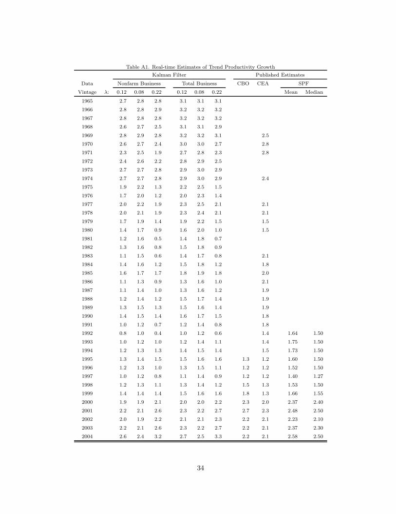
Table A1. Real-time Estimates of Trend Productivity Growth

Kalman Filter Published Estimates

Data Nonfarm Business Total Business CBO CEA SPF

Vintage λ: 0.12 0.08 0.22 0.12 0.08 0.22 Mean Median

1965 2.7 2.8 2.8 3.1 3.1 3.1

1966 2.8 2.8 2.9 3.2 3.2 3.2

1967 2.8 2.8 2.8 3.2 3.2 3.2

1968 2.6 2.7 2.5 3.1 3.1 2.9

1969 2.8 2.9 2.8 3.2 3.2 3.1 2.5

1970 2.6 2.7 2.4 3.0 3.0 2.7 2.8

1971 2.3 2.5 1.9 2.7 2.8 2.3 2.8

1972 2.4 2.6 2.2 2.8 2.9 2.5

1973 2.7 2.7 2.8 2.9 3.0 2.9

1974 2.7 2.7 2.8 2.9 3.0 2.9 2.4

1975 1.9 2.2 1.3 2.2 2.5 1.5

1976 1.7 2.0 1.2 2.0 2.3 1.4

1977 2.0 2.2 1.9 2.3 2.5 2.1 2.1

1978 2.0 2.1 1.9 2.3 2.4 2.1 2.1

1979 1.7 1.9 1.4 1.9 2.2 1.5 1.5

1980 1.4 1.7 0.9 1.6 2.0 1.0 1.5

1981 1.2 1.6 0.5 1.4 1.8 0.7

1982 1.3 1.6 0.8 1.5 1.8 0.9

1983 1.1 1.5 0.6 1.4 1.7 0.8 2.1

1984 1.4 1.6 1.2 1.5 1.8 1.2 1.8

1985 1.6 1.7 1.7 1.8 1.9 1.8 2.0

1986 1.1 1.3 0.9 1.3 1.6 1.0 2.1

1987 1.1 1.4 1.0 1.3 1.6 1.2 1.9

1988 1.2 1.4 1.2 1.5 1.7 1.4 1.9

1989 1.3 1.5 1.3 1.5 1.6 1.4 1.9

1990 1.4 1.5 1.4 1.6 1.7 1.5 1.8

1991 1.0 1.2 0.7 1.2 1.4 0.8 1.8

1992 0.8 1.0 0.4 1.0 1.2 0.6 1.4 1.64 1.50

1993 1.0 1.2 1.0 1.2 1.4 1.1 1.4 1.75 1.50

1994 1.2 1.3 1.3 1.4 1.5 1.4 1.5 1.73 1.50

1995 1.3 1.4 1.5 1.5 1.6 1.6 1.3 1.2 1.60 1.50

1996 1.2 1.3 1.0 1.3 1.5 1.1 1.2 1.2 1.52 1.50

1997 1.0 1.2 0.8 1.1 1.4 0.9 1.2 1.2 1.40 1.27

1998 1.2 1.3 1.1 1.3 1.4 1.2 1.5 1.3 1.53 1.50

1999 1.4 1.4 1.4 1.5 1.6 1.6 1.8 1.3 1.66 1.55

2000 1.9 1.9 2.1 2.0 2.0 2.2 2.3 2.0 2.37 2.40

2001 2.2 2.1 2.6 2.3 2.2 2.7 2.7 2.3 2.48 2.50

2002 2.0 1.9 2.2 2.1 2.1 2.3 2.2 2.1 2.23 2.10

2003 2.2 2.1 2.6 2.3 2.2 2.7 2.2 2.1 2.37 2.30

2004 2.6 2.4 3.2 2.7 2.5 3.3 2.2 2.1 2.58 2.50

34