price of liquidity in the reinsurance of fund returns

arX

iv:2

011.

1326

8v1

[q-

fin.

MF]

26

Nov

202

0

Working

pape

r

Price of liquidity in the reinsurance offund returns

David Saunders

Department of Statistics and Actuarial Science, University of Waterloo, Waterloo, Canada

[email protected]

Luis Seco

CEO Sigma Analysis & Management and Department of Mathematics, University of Toronto,

Toronto, Canada

[email protected]

Markus Senn

Department of Mathematical Finance, Technical University Munich, Munich, Germany

[email protected]

Abstract

This paper aims to extend downside protection to a hedge fund investment portfolio based on

shared loss fee structures that have become increasing popular in the market. In particular, we

consider a second tranche and suggest the purchase of an upfront reinsurance contract for any

losses on the fund beyond the threshold covered by the first tranche, i.e. gaining full portfolio

protection. We identify a fund’s underlying liquidity as a key parameter and study the pricing of

this additional reinsurance using two approaches: First, an analytic closed-form solution based

on the Black-Scholes framework and second, a numerical simulation using a Markov-switching

model. In addition, a simplified backtesting method is implemented to evaluate the practical

application of the concept.

Keywords: first-loss, hedge funds, liquidation barrier, portfolio downside protection, port-

folio reinsurance

http://arxiv.org/abs/2011.13268v1

Working

pape

r

Price of liquidity in the reinsurance of fund returns –1–

1 Introduction

The low interest rate environment, uncertain and fragile political climate and cost pressure

are main drivers for today’s challenging market environment. It is increasingly difficult for

hedge fund managers to justify high fees for return performances that tend not to be superior

to alternative low-cost investment opportunities, e.g. ETFs. A hedge fund’s capability of

deliberately incorporating more risk by either adding new risk sources or including riskier

positions poses an attractive alternative for investors to diversify their existing investment

portfolio. Nonetheless, weak performance, more difficult and volatile markets, and pressure to

raise assets combined with the investor’s call for better alignment of interest have resulted in

new fee structures in the hedge fund industry. Managers offer downside protection by insuring

investments in the hedge fund in return for a bigger share in generated profits. These fee

structures are commonly referred to as ‘first-loss’, ‘shared-loss’ or ‘shared-profit’.

In traditional fee structures the manager receives a flat 2% management fee and a perfor-

mance fee of 20% of net profits (known as ‘2 and 20’). Even though the ‘2 and 20’ concept is

commonly applied, other fixed and variable fee combinations are possible, e.g. Escobar et al.

(2017) suggest an optimal equilibrium in management and performance fees by optimizing the

commonly used Sharpe-Ratio to maximize the utility of both the manager and investor alike.

Nonetheless new fee structures in the form of first-loss schemes are emerging. There are several

versions of the first-loss principle, but the basic framework has the following features in com-

mon: the manager provides downside protection by covering the first tranche of portfolio losses

in return for a higher participation rate in case of a positive fund performance. In contrast to

traditional fee structures, a first-loss structure might allow a manager to raise the performance

fee to 50% by insuring losses up to 10% of the initial investment, i.e. providing protection for

the first tranche of portfolio losses. He and Kou (2018) derive trading strategies with a first-loss

structure based on cumulative prospect theory and conclude that certain parameter combina-

tions result in increasing utility for both the manager and the investor while reducing the risk of

an investment portfolio. However, in other cases, the traditional fee structure produces higher

investor utility. Djerroud et al. (2016) price the contract using risk-neutral valuation, thereby

obtaining the ‘fair’ level of the performance fee. Bhaduri et al. (2018) extend the traditional

first-loss principle by introducing a minimum return guarantee in addition to covering the first

tranche of losses in a portfolio. The investment resembles a coupon bond, with a guaranteed

minimum return (fixed part) and performance dependent return net of accrued fees (variable

part).

Working

pape

r


Independent of applied fee structures, hedge funds are often subject to so-called liquidation

barriers. These barriers can be introduced exogenously, i.e. they are investor demanded or

endogenously, i.e. the manager sets an internal barrier. They represent a commonly known

option to protect investors from negative fund performances. Once poorly performing funds

breach the liquidation barrier, their operations shut down to prevent further losses for the

investors. Hodder and Jackwerth (2007) analyze the effects of a shutdown or liquidation barrier

on the risk-taking behavior of the manager as another option to provide downside protection

for the investor. They find a significant change in the willingness to take on riskier positions

when the fund performance is close to the barrier.

Our approach aims to extend the protection beyond the first tranche of losses by considering

a second one that insures the investor against all losses, not just the first level. The interest

in this second layer of protection is manifold. On the one hand, investors may have a different

appetite for the second layer of losses from a third-party reinsurer, therefore creating a financial

transaction between investor and reinsurer. On the other hand, even if investors’ risk appetites

lead them to accept this second tranche of losses, or if reinsurance cost is deemed too high, there

may be regulatory reasons for this tranche to be outsourced to a third party, e.g., if the investor

is an insurance company subject to capital ratios linked to a loss profile that regulators may

penalize in excess of the external reinsurance cost. In any case, whilst most related research

focuses on optimizing fee structures in a first-loss framework, little work has been done on

protecting losses greater than the first tranche. We address the subject of providing additional

downside protection that goes beyond the insurance of the first tranche of losses.1

Theoretically, by introducing a liquidation barrier at the lower end of the first tranche, the

investor gains full portfolio protection. In this setting, the liquidation is triggered as soon as

the portfolio value breaches the barrier, in which case the manager compensates for all resulting

losses. In practice however, the investor is exposed to gap risk, arising from the inability of

the manager of the investment structure to liquidate the portfolio before losses exceed the

protection level of the first tranche. The risk premium that is relevant in the valuation of the

second loss tranche, i.e. pricing further downside protection, should reflect this exposure to

gap risk. Two related market events can give rise to this exposure; first, a situation where loss

momentum is higher than the manager’s ability to liquidate the portfolio in a timely manner.

The fund is exposed to price fluctuations from the moment when the fund value first hits the

1A similar payoff in a different financial contract is afforded to investors in variable annuities, who may receivea minimum guaranteed rate of return, together with fractional participation in the upside of an investmentportfolio managed by an insurance company.

Working

pape

r


barrier, at which point the manager is aware of the situation and starts the liquidation of all

assets, through to the end of the liquidation process. Second, a situation where the liquidity

of the underlying assets is low, to the point that an orderly liquidation of the portfolio extends

in time beyond the liquidation barrier and assets can continue to lose value. Whereas highly

liquid assets (e.g. most stocks, futures or certain bonds) can be liquidated within seconds or

minutes to minimize the gap risk, illiquid assets (e.g. real estate or certain OTC products) take

time to liquidate and are exposed to market risk over a longer period of time. As the manager

only covers losses up to the barrier in both cases, the investor is exposed to the gap risk and

losses can exceed the first tranche.

We analyze a contract in which an investor pays an upfront premium to a reinsurance party

and in exchange gains full portfolio protection net of fees. The contribution of this paper

is a method of computing the premium for the reinsurance as a function of the liquidity of

the underlying portfolio. Assuming risk-neutral valuation and a geometric Brownian motion

for the value of the underlying portfolio, we derive a closed-form expression for the premium.

In addition to the analytical approach, we conduct a numerical simulation using a Markov-

switching model as an alternative. Furthermore, we provide some sensitivity analysis with

respect to certain market parameters and variations of the initial setting.

The remainder of the paper is structured as follows. Section two elaborates on established

first-loss concepts and introduces our modifications. In section three, we consider the analytical

model using a geometric Brownian motion and derive a closed-form solution. The fourth section

contains a simulation in a Markov-Switching model. In section five, we present numerical

results. Section six is dedicated to backtesting the introduced models. Section seven concludes.

We wish to express our gratitude to Michael Ege for some very useful insights on the business

aspects of this paper as well as for interesting comments of earlier drafts

2 Hedge fund fee structures

2.1 Established first-loss framework

First-loss schemes were established several years ago but have found rising interest in recent

years2. Especially in the aftermath of the financial crisis, managers lacked investor confidence.

2https://www.marketwatch.com/story/more-hedge-funds-lured-to-new-source-of-capital-2011-05-23?pagenumber=1 for an article on Dow Jones & Company’s MarketWatch about rising interest infirst-loss schemes in recent years from May 23, 2011 and https://www.bloomberg.com/news/articles/2018-04-23/paulson-levers-up-bets-seeking-big-fees-while-risking-his-money for a Bloomberg article on recent first-loss

Working

pape

r


The first-loss principles not only signal a manager’s dedication, as his own funds are at stake,

but also allow smaller funds and those without a long track record to attract new investors

and quickly grow assets in the early seeding phase. However, the first-loss scheme comes with

a price. The manager provides downside protection by covering the first tranche of portfolio

losses in return for a higher participation rate in the event of a positive fund performance.

Whereas in traditional fee structures the manager receives a flat 2% management fee and a

20% performance-dependent fee on net profits (known as ‘2 and 20’), a first-loss structure

might allow a manager to raise the performance fee to 50% by insuring losses up to 10% of the

initial investment.

There exists a variety of first-loss variations. In this paper, we are closely following the

framework of Djerroud et al. (2016). The fund value Xt consists of two parts, the manager’s

part VM(t) and the investor’s part VI(t), where Xt = VI(t)+VM(t). The payoffs at the terminal

time T are defined as follows:

VI(T ) =

XT −mMX0 − αM(XT −mmX0 −X0)+

(1−mM)X0

XT + (cM −mM )X0

whenXT ≥ X0

when (1− cM)X0 ≤ XT ≤ X0

whenXT ≤ (1− cM)X0

VM(T ) =

mMX0 + αM(XT −mmX0 −X0)+

mMX0 − (X0 −XT )

mMX0 − cMX0

whenXT ≥ X0

when (1− cM)X0 ≤ XT ≤ X0

whenXT ≤ (1− cM)X0

or, in more condensed form:

VI(T ) = XT −mMX0 − αM [XT −mmX0 −X0]+ + [X0 −XT ]

+ − [(1− cM)X0 −XT ]+ (1)

VM(T ) = mMX0 + αM [XT −mmX0 −X0]+ − [X0 −XT ]

+ + [(1− cM)X0 −XT ]+ (2)

where X0 is the initial investment, αM is the performance dependent fee, mM is the flat manage-

ment fee and cM the managerial deposit, i.e. (1 − cM)X0 is the lower level of the first tranche

insurance. In other words, the manager compensates the investor in the event of negative

performance with up to cM of the initial investment.

The payoff functions form the base case of our derivative-pricing framework. The investor

holds a long position representing her investment, i.e. the fund’s assets net fees (XT −mMX0),

related news from April 23, 2018.

Working

pape

r


a short position in a call option on the fund’s assets with strike mMX0 + X0 representing

potential performance dependent fees, a long position in a put option on the fund’s assets with

strike X0 representing first-loss insurance by the manager and a short position in a put option

on the fund’s assets with strike (1− cM)X0 representing the cap on the manager’s deposit, i.e.

the manager’s limited liability in the event of a negative fund performance beyond the first-loss

protection. The manager holds the respective counterparts, i.e. a long call option, a long put

option and a short put option.

2.2 Modified framework: Reinsurance

Theoretically, by introducing a liquidation barrier at the level of the lower end of the man-

agerial deposit (or first tranche of losses), i.e. at K = (1 − cM)X0 the investor gains full

portfolio protection. In this setting, the liquidation is triggered as soon as the portfolio value

breaches the barrier, in which case the manager compensates for all resulting losses. As noted

above, however, in practice the investor is exposed to gap risk owing to potential delays when

liquidating the portfolio, e.g. due to market conditions or the illiquid nature of the instruments

in the investment portfolio.

Consider the situation in which the investor pays a premium to a third party reinsurer, in

return for protection from losses not covered by the manager. Denote the value of the reinsurer’s

position by VR(t). The fund value now follows Xt = VI(t) + VM(t) + VR(t), where the payoff

functions are defined as follows:

VI(T ) =

XT − (mM +mR · erT )X0 − αM (XT −mMX0 −X0)+

(1−mM −mR · erT )X0

whenXT ≥ X0

whenXT ≤ X0

VM (T ) =

mMX0 + αM (XT −mMX0 −X0)+

mMX0 − (X0 −XT )

mMX0 − cMX0

whenXT ≥ X0

when (1− cM )X0 ≤ XT ≤ X0

whenXT ≤ (1− cM )X0

VR(T ) =

mR · erT ·X0

mR · erT ·X0 − ((1 − cM )X0 −XT )

whenXT ≥ (1− cM )X0

whenXT ≤ (1− cM )X0

where X0 is the initial investment, αM is the performance dependent fee, mM is the flat

management fee and cM the managerial deposit, i.e. (1 − cM)X0 is the lower level of the first

tranche insurance, mR is the upfront premium for the full portfolio insurance and r is the

Working

pape

r


risk-free interest rate. Written more compactly:

VI(T ) = XT − (mM +mR · erT )X0 − αM [XT −mMX0 −X0]+ + [X0 −XT ]

+ (3)

VM(T ) = mMX0 + αM [XT −mMX0 −X0]+ − [X0 −XT ]

+ + [(1− cM)X0 −XT ]+ (4)

VR(T ) = mR · erT ·X0 − [(1− cM)X0 −XT ]+ (5)

Note we assume that the investor cannot redeem her investment during the investment horizon,

e.g. due to an imposed lock-up period even though it might be optimal to prematurely withdraw

from the arrangement from the point of view of the investor (see Chen et al. (2016) and Meng

and Saunders (2018), who analyze optimal stopping times). The payoff functions (3) to (5)

extend the functions in (1) and (2). The short position representing the cap on the manager’s

deposit is transferred from the investor to the reinsurer, i.e. the investor gains full portfolio

protection net of fees. However, the investor is subject to another future liability representing

the premium (mR · erT ·X0). Despite the full portfolio protection, the investor is now facing a

certain credit risk, as she now relies on the financial solvency of the reinsurance in the event of

a negative fund performance. We assume no default and thus neglect the credit risk. Note that,

from the manager’s perspective, nothing changes, as (2)=(4). The transaction only involves

the investor and reinsurer.

As this paper focuses on the upfront premium paid by the investor, we will be placing the

emphasis on the payoff of the reinsurance in (5) hereafter. Note that the payoff function in

(5) is defined assuming no liquidation barrier, i.e. computed using the terminal fund value at

the end of the investment horizon T . In order to incorporate the aforementioned gap risk and

thus reflect a fund’s level of liquidity, we need some alterations of the payoff function of the

reinsurance stated in (5). We set a liquidation barrier at the lower end of the first tranche,

i.e. at K = (1 − cM)X0. If the fund value breaches this barrier at any time τ ∈ (0, T ), all

operations stop and the remaining assets are fully liquidated. Reflecting a fund’s underlying

level of liquidity, we introduce the parameter Θ. As a measure of liquidity, Θ is defined as the

time a fund needs to liquidate its assets. The payoff function is defined as follows:

VR(τ +Θ) = mR · er(τ+Θ)X0 − [K −Xτ+Θ]+ τ ∈ (0, T ) (6)

where τ = inf{t > 0;Xt ≤ K}. In the event, that the fund value does not breach the liquidation

barrier, we have [K −X ]+X>K= 0, i.e. the reinsurer receives and keeps the full premium. The

benchmark value that we use is Θ = 1252

, i.e. one day until full liquidation of the fund. In

Working

pape

r


practice, the liquidation process of a fund heavily depends on the composition of its financial

assets and the liquidation time is different for each asset. In the following sections we derive

the price of the upfront premium depending on the fund’s liquidity.

3 Analytic Valuation using Geometric Brownian Motion

Let the hedge fund performance X = {Xt}t∈[0,T ] follow a geometric Brownian motion. Under

the risk-neutral measure Q, we have

dXt = Xt · (rdt+ σdW̃t)

⇒ Xt = X0 · e(r−12σ2)t+σW̃t (7)

where r is the risk-free rate, σ > 0 is the fund’s volatility and W̃t is a Q-Brownian motion. As

above, let τ := inf{0 < t ≤ T : Xt = K} be the stopping time at which the fund value hits the

barrier K = (1 − cm) · X0. At time τ , the fund is shut down and all its assets are liquidated.

Using (7), we have

τ := inf{0 < t ≤ T : Xt = K} = inf{0 < t ≤ T : Yt = a} (8)

where Yt = (r − 1

2σ2)

︸︷︷︸

µ

t+σW̃t and a = ln(

KX0

)

. For fixed a, the first hitting time τ in (8) follows

an inverse Gaussian distribution (see Kwok (2008)) τ ∼ IG(µ∗, λ∗) where µ∗ = aµ, λ∗ = a2

σ2 and

the density function f is:

f(τ, µ∗, λ∗) =

√

λ∗

2πτ 3exp

(

−λ∗(τ − µ∗)2

2(µ∗)2τ

)

⇔ f(τ, a, µ) =|a|

σ√2πτ 3

exp

(

−(a− µτ)2

2σ2τ

)

(9)

We derive the value of the upfront premium mR as a function of a fund’s liquidity by using

the fair value approach stated in Djerroud et al. (2016), where the fair value for the premium

is obtained by setting the present value of the expected payoff equal to the initial investment,

i.e. VR(0) = 0. In our setting we have:

VR(0) = EQ[e−r(τ+Θ)VR(τ +Θ)] = 0 (10)

Working

pape

r


The payoff made by the reinsurer is that of a put option issued at time τ with strike

K = (1− cM)X0 and exercise time τ +Θ. For simplicity and without loss of generality, we set

the initial investment to X0 = 1. From (6), the terminal value of the reinsurer at time τ + Θ

is thus:

VR(τ +Θ) = mR · er(τ+Θ)X0 − [K −Xτ+Θ]+ = mR · er(τ+Θ) − [K −Xτ+Θ]

+ (11)

At time τ , the time of issuance of the put option, the value of the reinsurer’s position is:

VR(τ) = EQ[e−rΘ · VR(τ +Θ)|Fτ ] = mR · erτ − V1(Θ)

By definition K = Xτ , as the option is issued when the fund breaches the barrier. Thus,

V1(Θ) follows the well-known Black-Scholes option formula:

V1(Θ) = EQ[e−rΘ[K −Xτ+Θ]

+|Fτ ] = K(e−rΘ ·N(−d2)−N(−d1))

with d1 =(r + 1

2σ2)

√Θ

σ, d2 = d1 − σ

√Θ (12)

where N(·) is the standard normal cumulative distribution function. Note that V1(Θ) does not

depend on τ , but solely on Θ, i.e. V1(Θ) is a function of liquidity. At time t = 0, the initial

value of the reinsurer is:

VR(0) = EQ[e−rτ · VR(τ)|F0] = mR − V1(Θ) · EQ[e

−rτ |F0] = mR − V1(Θ) · V2(T ) (13)

where

V2(T ) = EQ[e−rτ |F0] =

∫ T

0

e−rtf(t) dt (14)

The above integral can be evaluated analytically (see Kwok (2008)):

V2(T ) =

(K

X0

)α+

N

δln(

KX0

)

+ βT )

σ√T

+

(K

X0

)α−

N

δln(

KX0

)

− βT )

σ√T

with β =

√

(r − σ2

2)2 + 2rσ2, α± =

r − σ2

2± β

σ2and δ = sign

(

ln

(X0

K

))

. (15)

Working

pape

r


We thus obtain:

mR = V1(Θ) · V2(T ) (16)

The premium is composed of two parts: V1(Θ) represents the value of the issued option and

V2(T ) incorporates the (discounted) probability of breaching the liquidation barrier throughout

the entire investment horizon T .

Note, some practitioners might prefer results for a model which is fitted to historical data.

Hence, we replace the risk-free drift with an empirical drift b, which implies that log(Xt+∆

Xt) ∼

N((b − 12σ2)∆, σ2∆) = N(µemp∆, σ2

emp∆) for a daily setting with ∆ = 1252

as log-returns are

normally distributed. Best estimates for drift and volatility are σ̂ = σemp and b̂ = µemp+12σ2emp,

where µemp = 252 · 1N

N∑

n=1

Rn and σemp =

√

252 · 1N−1

N∑

n=1

(Rn − µemp) with daily log-return

Rn. The empirical yearly returns µemp and volatility σemp for selected hedge fund indices (see

details in section 4) can be found in table 13. We would like to point out that we are not

pricing the contract using the risk-neutral measure Q in the following. The crucial assumptions

needed to justify the replication arguments that underlie risk-neutral valuation might not hold

in the hedge fund context, e.g. as we specifically allow illiquid asset classes, the arbitrage-free

dynamic hedging strategy underlying the classic Black-Scholes framework is hardly attainable.

Therefore, we evaluate the present value of the expected payoff (represented by V P1 (Θ) in

equation (17)). Investors might be interested in this value, which is still available in closed-

form. For equation (12) we have:

V P1 (Θ) = EP[e

−rΘ[K −Xτ+Θ]+|Fτ ] = K(e−rΘ ·N(−d2)− e(b−r)Θ ·N(−d1))

with d1 =(b+ σ2

2)√Θ

σ, d2 = d1 − σ

√Θ (17)

and for equation (15) we have:

V P2 (T ) =

(K

X0

)α+

N

δln(

KX0

)

+ βT )

σ√T

+

(K

X0

)α−

N

δln(

KX0

)

− βT )

σ√T

with β =

√

(b− σ2

2)2 + 2rσ2, α± =

(b− σ2

2)± β

σ2and δ = sign

(

ln

(X0

K

))

. (18)

3Estimating drift rates is notoriously difficult and nearly impossible to do in practice (see Merton (1980)for the original paper on the problem). We follow a simple approach and use mean and standard deviation oflog-returns.

Working

pape

r


We thus obtain:

mPR = V P

1 (Θ) · V P2 (T ) (19)

4 Valuation in a Markov-switching framework

We consider a Markov-switching model and evaluate the payoff of the reinsurance to com-

pute the premium mR. Markov-switching or regime-switching models were first introduced by

Hamilton (1989) and have since found regular application in the financial world. These models

create returns similar to actual hedge fund returns and show typical hedge fund characteristics,

i.e. skewness, volatility clusters and fat tails. We assume a two state Markov-switching model

with state space S = {1, 2} for the continuous-time Markov chain ε(t), where state 1 represents

the ‘normal’ market and state 2 the ‘stressed’ market. ε(t) is generated by the intensity matrix

Q =

−λ1 λ1

λ2 −λ2

,

where λ1 and λ2 are the transition rates for switching states. The fund value satisfies the

following stochastic differential equation:

dXt = Xt · (µε(t)dt+ σε(t)dWt) , X0 > 0

where ε(t) ∈ {1, 2} and µε(t) and σε(t) represent the respective state’s return rate and volatility.

In order to use the risk-neutral martingale pricing methodology, we need an equivalent martin-

gale measure Q. We follow the approach in Henriksen (2011) by using the Girsanov theorem

and assume unchanged transition probabilities under the risk-neutral measure Q (see Bollen

(1998) and Hardy (2001) for the same approach). The resulting price process for constant r is

given by:

Xt = X0 · exp{∫ t

0

r − 1

2σ2ε(u))du+

∫ t

0

σε(u)dW̃u

}

, X0 > 0.

For another approach see Elliott et al. (2005), where a regime switching Esscher transform

is applied to obtain an equivalent measure. Note, the Markov-switching modeled market is

incomplete, as there is an additional stochastic dimension in form of the regime switching and

Working

pape

r


a unique Q measure cannot be determined (for a proof see for example Elliott and Swishchuk

(2007)).

When performing simulations, we implement the following discretized version of the regime-

switching Markov process on an equidistant grid:

Xti = X0 · eRti , ∀i ∈ {0, ..., k}, X0 > 0

Rti = Rti−1+

(

(r − 1

2σ2ε̃(ti)

)∆ + σε̃(ti)

√∆ · ηti

)

, Rt0 = 0

where 0 = t0 < t1 < ... < tk = T , ∆ ≡ ∆tj := tj+1 − tj = T/k, ηti are i.i.d. standard normal

random variables and ε̃(t) is a discretization of the continuous-state Markov-chain ε(t) with

transition matrix:

P =

(1− p) p

q (1− q)

,

where p and q are the transition probabilities for switching from one state to the other:

p = P(ε̃(ti+1) = 1|ε̃(ti) = 2)

q = P(ε̃(ti+1) = 2|ε̃(ti) = 1)

The time-homogeneous Markov chain ε̃ has stationary distribution π1 =q

q+pand π2 =

pq+p

. We

assume daily time steps and consider one year to be made up of 252 trading days, i.e. ∆ = 1252

.

For the numerical approach, we simulate N = 100, 000 paths of the discretized Markov-

switching process4. For each sample path Xnt , n = 1, ..., N , the reinsurer’s value at time

t = τ +Θ is given by:

V nR (τ

n +Θ) = mnR · er(τn+Θ)X0 − [K −Xn

τn+Θ]+. (20)

At time t = 0 the reinsurer’s value is thus:

V nR (0) = mn

RX0 − e−r(τn+Θ)[K −Xnτn+Θ]

+. (21)

Similar to the analytical valuation, we use the fair value approach stated in Djerroud et al.

(2016) to derive the upfront premium mR and set the present value of the expected payoff

4Simulations were conducted using MatLab and R.

Working

pape

r


equal to zero such that:

1

N

N∑

n=1

V nR (0) = 0 (22)

i.e. using equation (21) and X0 = 1 we find

1

N

N∑

n=1

(mRX0 − e−r(τn+Θ)[K −Xnτn+Θ]

+) = 0 (23)

We thus obtain:

mR =1

N

N∑

n=1

e−r(τn+Θ)[K −Xnτn+Θ]

+ (24)

The following illustrates the employed algorithm:

1) Simulate the (discretized) Markov chain ε̃n(t) for path n with state space S = {1, 2} for

t ∈ { 1252

, 2252

, ..., T } in a daily setting with 252 trading days where T = 1, i.e. one year.

2) Simulate the daily trajectory Xnt = X0 · eRn

t with Rnt = Rn

t−1+1

252· (r− 1

2σ2i )+

√1

252·σi ·η

where R0 = 0, η ∼ N(0, 1) and i ∈ {1, 2} denotes the state of the market.

3) If Xnt < 0.9X0 for any 0 < t < T , set the stopping time τn = inf{0 < t < T : Xn

t < 0.9X0}and use Xn

τn+Θ to evaluate the respective payoff and τn +Θ to discount the payoff.

4) Repeat step 1 to 3 a sufficient number of times (here N = 100, 000) and apply (24) to

find the expected upfront premium mR.

As it is preferable to decrease an estimate’s variance, we also apply the antithetic variates

method in our simulation. This method exploits the symmetry of the randomly generated

i.i.d. standard normal variables η ∼ N(0, 1) in step 1) of our algorithm above. It holds for

η ∼ N(0, 1), that ηd= −η and thus we can replace η by −η in step 1) without changing

the trajectory’s distribution. For the estimated trajectory Xnantithetic :=

Xnη +Xn

−η

2it holds, that

var(Xnantithetic) ≤ var(Xn) (see Kroese et al. (2013) for details).

Again, some practitioners might be interested in the actual discounted expected payoff of

their investment. Analogously to the previous section (GBM model), we replace the risk-free

drift with empirical yearly returns µ1,µ2 and volatility σ1,σ2 for selected hedge fund indices

(see details below), which can be found in Table 1. Note, the same arguments on the difficulty

of estimating empirical drifts and risk-neutral pricing from the previous section hold in the

Working

pape

r


Markov-switching model. We do not price the contract but evaluate the present value of the

expected payoff.

We fit the parameters of the Markov-switching model to real world historical data. To

obtain reasonable parameters and to cover most of the hedge fund universe, we analyze five

main hedge fund strategies: Equity Hedge, Equity Market Global, Neutral, Macro and Merger

Arbitrage. Saunders et al. (2013) use these strategies as proxies for all available strategies.

Our primary source of data was the open source database for daily fund returns operated by

Chicago based company Hedge Fund Research (HFR). The observation period started April 1,

2003 and ended December 28, 2018. Parameter values for µ1, µ2, p and q are estimated using

the well-known Baum-Welch algorithm (Baum et al. (1970)) in the R-routine ‘Baum-Welch’

from the package ‘HiddenMarkov’. As initial values for this maximum likelihood estimation, we

employ a heuristic proposed in Ernst et al. (2009). Finally, we use Viterbi’s algorithm to create

the most likely sequence of states (see Viterbi (1967) for details) and compute respective mean

returns and average all five strategies’ returns and transition probabilities. Another approach

to obtain the required parameters is the estimation by moment matching (see Höcht et al.

(2009) for details).

Figure 1 illustrates the resulting crisis periods for the exemplary HFRXEH index using the

heuristic and the Baum-Welch algorithm. Table 1 contains all analyzed HFRX indices and their

respective numerical parameters values and historical data for a single-regime (Black-Scholes)

market.

Working

pape

r


This figure illustrates the HFRXEH Equity Hedge Index between April 1, 2003 and December28, 2018. The top graph shows crisis periods in black using the crisis detection heuristic andthe bottom graph shows crisis periods using the Baum-Welch algorithm.

Figure 1: HFRXEH

Ticker HFRX Index Name Strategy p [in %] q [in %] µ1 [in %] µ2 [in %] σ1 [in %] σ2 [in %] µemp [in %] σemp [in %]HFRXGL Global Hedge Fund Global 1.67 7.49 8.54 -32.40 2.57 6.44 1.08 3.73HFRXM Macro\CTA Macro 1.87 7.79 4.84 -15.36 4.55 10.93 0.75 6.33HFRXEMN EH: Equity Market Neutral Neutral 1.13 6.09 1.12 -6.87 2.88 7.08 -0.20 3.85HFRXEH Equity Hedge Equity Hedge 2.02 6.19 11.25 -30.36 4.28 10.12 0.87 6.35HFRXMA ED: Merger Arbitrage Merger Arbitrage 2.07 15.70 5.46 -8.27 2.16 10.17 3.79 4.02mean 1.75 8.65 6.24 -18.65 3.29 8.95 1.26 4.86max 2.07 15.70 11.25 -6.87 4.55 10.93 3.79 6.35min 1.13 6.09 1.12 -32.40 2.16 6.44 -0.20 3.73

This table shows an overview of all HFRX indices for the period April 1, 2003 to December 28,2018. Parameters p, q, µ1/2, σ1/2 were obtained from the Baum-Welch algorithm. µemp and σemp

represent empirical returns and volatility for a single-regime (Black-Scholes) market.

Table 1: Overview HFRX

5 Results

We set the initial parameters for both approaches to the following values:

• T = 1 (one-year investment horizon)

• X0 = 1 (initial investment)

• K = (1-cM)X0 = 0.9 (liquidation barrier)

• r = 0.01 (risk free rate)

In the following the unit of the liquidity measure Θ is one day, i.e. Θ = 1 represents a daily

liquidation window and was implemented in the model as 1252

.

Working

pape

r


5.1 Analytical results using GBM approach

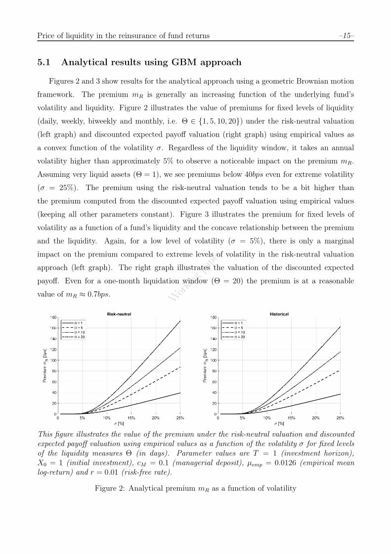
Figures 2 and 3 show results for the analytical approach using a geometric Brownian motion

framework. The premium mR is generally an increasing function of the underlying fund’s

volatility and liquidity. Figure 2 illustrates the value of premiums for fixed levels of liquidity

(daily, weekly, biweekly and monthly, i.e. Θ ∈ {1, 5, 10, 20}) under the risk-neutral valuation

(left graph) and discounted expected payoff valuation (right graph) using empirical values as

a convex function of the volatility σ. Regardless of the liquidity window, it takes an annual

volatility higher than approximately 5% to observe a noticeable impact on the premium mR.

Assuming very liquid assets (Θ = 1), we see premiums below 40bps even for extreme volatility

(σ = 25%). The premium using the risk-neutral valuation tends to be a bit higher than

the premium computed from the discounted expected payoff valuation using empirical values

(keeping all other parameters constant). Figure 3 illustrates the premium for fixed levels of

volatility as a function of a fund’s liquidity and the concave relationship between the premium

and the liquidity. Again, for a low level of volatility (σ = 5%), there is only a marginal

impact on the premium compared to extreme levels of volatility in the risk-neutral valuation

approach (left graph). The right graph illustrates the valuation of the discounted expected

payoff. Even for a one-month liquidation window (Θ = 20) the premium is at a reasonable

value of mR ≈ 0.7bps.

This figure illustrates the value of the premium under the risk-neutral valuation and discountedexpected payoff valuation using empirical values as a function of the volatility σ for fixed levelsof the liquidity measures Θ (in days). Parameter values are T = 1 (investment horizon),X0 = 1 (initial investment), cM = 0.1 (managerial deposit), µemp = 0.0126 (empirical meanlog-return) and r = 0.01 (risk-free rate).

Figure 2: Analytical premium mR as a function of volatility

Working

pape

r


This figure illustrates the value of the premium under the risk-neutral valuation and discountedexpected payoff valuation using empirical values as a function of the liquidity measure Θ (indays) for fixed levels of volatility σ and the empirical volatility σemp = 0.0486. Parametervalues are T = 1 (investment horizon), X0 = 1 (initial investment), cM = 0.1 (managerialdeposit), µemp = 0.0126 (empirical mean log-return) and r = 0.01 (risk-free rate).

Figure 3: Analytical premium mR as a function of liquidity

5.2 Numerical results using Markov-switching approach

Figures 4 to 6 show results for the numerical approach using a simulation with a Markov-

switching model as underlying framework. The stationary distribution π = (π1, π2) = ( qp+q

, pp+q

) =

(0.8317, 0.1683) for p = 0.0175 and q = 0.0865 indicates a high probability of the market being

governed by state 1, i.e. the ‘good’ market environment. Hence, Figures 4 and 5 illustrate the

value of the premium depending on σ1 for fixed levels of σ2 and different levels of liquidity (Θ

in days). Similar to results in the GBM section, figure 4 (initial state is ‘good’) illustrates the

premium as a convex function of a fund’s volatility. For low levels of volatility in both states

(σ1/2 ≤ 5%) we find a marginal impact on the premium. However, assuming very liquid assets

(Θ = 1) even for extreme values in both states, i.e. σ1/2 = 25% the premium is significantly

lower (mR ≈ 74bps) than in the single-regime model (for σ = 25% we find mR ≈ 170bps). For

lower levels of volatility in state 1 (σ1 ≤ 10%), the volatility of state 2 has much higher impact

on the premium compared to a high volatility in state 1 (σ1 ≈ 25%). Figure 5 illustrates results

for a market with initial state ‘stressed’. As expected, the premiums are higher than when as-

suming a ‘good’ initial market. In figure 6, we see the premium using the discounted expected

payoff valuation for empirical values depending on the initial state of the market. Assuming a

‘stressed’ initial market, the premium is roughly twice as high as for a ‘good’ initial market.

Working

pape

r


Except for a daily liquidation window, even for ‘stressed’ market, the premium is below the the

premium using a single-regime model (see figure 3). For a one-month liquidation window, pre-

miums are approx. 0.3bps for a ‘good’ market and approx. 0.5bps for a ‘stressed’ market. For

comparison: the premium for the same level of liquidity in the single-regime model is approx.

0.7bps. The results indicate, that the selection of the applied model matters substantially for

an investor. As the actual state of the market is not an observable variable, we also include

a ‘weighted average’. The Baum-Welch algorithm indicates that the HFRX indices in table 1

spent an average of 84.27% in the ‘good’ state during the period between April 1, 2003 and

December 28, 2018. Using this number as a proxy for the probability, that the market is in a

‘good’ state, we compute a ‘weighted average premium’.

Working

pape

r


This figure illustrates the value of the premium under risk-neutral valuation as a function of thevolatility σ1 for fixed levels of volatility σ2 for different liquidation windows (Θ in days), whenthe state of the initial market is ‘good’, i.e. ε̃(0) = 1. Parameter values are T = 1 (investmenthorizon), X0 = 1 (initial investment), cM = 0.1 (managerial deposit), r = 0.01 (risk-free rate),p = 0.0175 (probability of switching from ‘good’ to ’stressed’ state) and q = 0.0865 (probabilityof switching from ‘stressed’ to ‘good’ state).

Figure 4: Numerical premium mR as a function of volatility - initial market ‘good’

Working

pape

r


This figure illustrates the value of the premium under risk-neutral valuation as a functionof the volatility σ1 for fixed levels of volatility σ2 for different liquidation windows (Θ indays), when the state of the initial market is ‘stressed’, i.e. ε̃(0) = 2. Parameter values areT = 1 (investment horizon), X0 = 1 (initial investment), cM = 0.1 (managerial deposit),r = 0.01 (risk-free rate), p = 0.0175 (probability of switching from ‘good’ to ‘stressed’ state)and q = 0.0865 (probability of switching from ‘stressed’ to ‘good’ state).

Figure 5: Numerical premium mR as a function of volatility - initial market ‘stressed’

Working

pape

rThis figure illustrates the value of the premium under the discounted expected payoff valuationusing empirical values as a function of the liquidity measure Θ (in days) for the empiricalvolatility σ1 = 0.0329 and σ2 = 0.0895 for both ‘good’ initial market, i.e. ε̃(0) = 1, and‘stressed’ initial market, i.e. ε̃(0) = 2. The ‘weighted average’ uses a probability of 0.8427, thatthe market is in a ‘good’ state. Parameter values are T = 1 (investment horizon), X0 = 1(initial investment), cM = 0.1 (managerial deposit), r = 0.01 (risk-free rate), µ1 = 0.0624(return ‘good’ state), µ2 = −0.1865 (return ‘stressed’ state), p = 0.0175 (probability of switchingfrom ‘good’ to ‘stressed’ state) and q = 0.0865 (probability of switching from ‘stressed’ to ‘good’state).

Figure 6: Numerical premium mR as a function of volatility

6 Backtesting

6.1 Setup and assumptions

This Section elaborates on the backtesting of the suggested premium in the previous Sec-

tions. It aims to evaluate the practical application of the concept and how it would have

performed in recent years. As the concept of insuring hedge fund portfolio losses beyond the

first-loss tranche is completely new and no work has been done so far, there exist no prede-

fined ways to evaluate the backtest or benchmark our results of the proposed premium to other

approaches. Hence, this Section serves as a first starting point in improving the practical appli-

cation of the concepts mentioned in this paper. The general idea of backtesting in this context

Working

pape

r


is the evaluation of the computed premium using real world historical data. In order to obtain

valid results, the look-ahead bias has to be avoided. This bias occurs when at certain times

data or information, which was not available at the actual point in time of the event, is used

for a simulation or evaluation of those events. The HFRX data set used for table 1 is the main

source of data used here. It contains daily returns from April 1, 2003 until December 28, 2018.

Fund-depending parameters, e.g. returns, volatility and transition probabilities are determined

using the HFRX data set. The annualized risk-free rates r are extracted from the Kenneth R.

French website5, which provides 1-month TBill returns starting in July, 1926. The following

list describes the backtesting approach implement in this Section:

1) Define a starting point, investment target (e.g. HFRXGL) and crucial parameters (i.e.

liquidity measure Θ, fees, managerial deposit cM ,initial investment X0,...).

2) Estimate all parameters needed to compute the premium for a one-year insurance at the

specific point in time depending on the predefined valuation approach, i.e. geometric

Brownian motion framework or Markov-switching framework.

3) Determine the premium and thus the initial values for the investor, the manager and the

reinsurer at the specific point in time.

4) Let the hedge fund performance develop according to the historical data.

5a) In the event that the fund value breaches the barrier at any time during the one-year

investment horizon, all assets are liquidated and the payoff is evaluated using the final

value depending on the underlying liquidity.

5b) In the event of no breach, evaluate the one-year performance at the end of the period.

6) (Only following step 5b)) Start a new investment period until the liquidation event occurs

or a predefined stopping criterion is reached, e.g. when no historical data is available

anymore.

Note, we are using the risk-neutral approach. The following elaborates how the specific param-

eters at a certain point in time are obtained and how the fund performance is evaluated. First,

we illustrate the implemented algorithm: Let the initial investments for the investor XI(i), the

5See http://mba.tuck.dartmouth.edu/pages/faculty/ken.french/data_library.html for details

Working

pape

r


manager XM(i) and the reinsurer XR(i) for investment period i, i = 1, 2, ..., T − 1 be given by

XI(i) = V̂I(i− 1) = Xi,

XM(i) = V̂M(i− 1),

XR(i) = V̂R(i− 1),

where for i = 0, the following values are set: XI(0) = X0, XM(0) = 0 and XR(0) = 0. Note, in

this paper X0 = 1. At the beginning of the investment period i the premium mRiis computed

and the initial values for the investor VI(i), the manager VM(i) and the reinsurer VR(i) for

investment period i, i = 0, 1, ..., T − 1 are given by

VI(i) = (1−mRi)XI(i),

VM(i) = XM(i),

VR(i) = XR(i) +mRiXI(i).

The final values for the investor V̂I(i), the manager V̂M(i) and the reinsurer V̂R(i) for investment

period i, i = 0, 1, ..., T − 1 are given by

V̂I(i) = Xi,i+1 −mRierXI(i)− αM [Xi,i+1 −XI(i)]

+ + [XI(i)−Xi,i+1]+,

V̂M(i) = erVM(i) + αM [Xi,i+1 −XI(i)]+ − [XI(i)−Xi,i+1]

+ + [(1− cM)XI(i)−Xi,i+1]+,

V̂R(i) = erVR(i)− [(1− cM)XI(i)−Xi,i+1]+,

where Xi,i+1 denotes the one-year price development of the initial investment XI(i) in period i,

hence it is the final value of the initial investment XI(i) for this period, which is used as initial

investment in period (i+1). Note, for a one-period investment horizon and no flat management

fee (mM = 0), the equations above yield equations (3) to (5). Now, if for any τ ∈ [0, 1] it holds

that Xi,i+τ ≤ (1− cM)Xi = (1− cm)XI(i) the hedge fund is liquidated depending on Θ, e.g. in

this paper Θ ∈ { 1252

, 5252

, 10252

, 20252

}, and the final value is set to the following:

V̂I(i) =Xi,i+τ+Θ −mRier(τ+Θ)XI(i)− αM [Xi,i+τ+Θ −XI(i)]

+ + [XI(i)−Xi,i+τ+Θ]+,

V̂M(i) = er(τ+Θ)VM(i) + αM [Xi,i+τ+Θ −XI(i)]+ − [XI(i)−Xi,i+τ+Θ]

+

+ [(1− cM)XI(i)−Xi,i+τ+Θ]+,

V̂R(i) = er(τ+Θ)VR(i)− [(1− cM)XI(i)−Xi,i+τ+Θ]+.

Working

pape

r


Note, we employ daily time steps in our backtest. This allows for a smoother performance

graph.

As already mentioned, the approach is a simplification and several assumptions and speci-

fications are made:

- Rolling windows: Premiums are computed based on parameters obtained from a two-year

rolling window. In the geometric Brownian motion approach, the estimated volatility is

simply the sample volatility. For the Markov-switching approach, we use the Baum-Welch

algorithm according to Section 4 to estimate volatility and transition probabilities.

- No reinvestment: This applies to the manager and reinsurer only. All premiums and per-

formance fees are not reinvested in the hedge fund but transferred to a riskless investment

account. In other words, the upfront premiums are compounded using the risk-free rate

at the time of occurrence. Premiums from following investment periods are added to the

account and compounded until either the liquidation event is triggered or the ultimate

investment horizon is reached. We are aware of the fact that in practice the premiums

collected by an insurance company are subject to individual asset/liability management

(ALM) processes. In some cases it is even plausible to reinvest parts or the entire pre-

mium in the fund and participate in upside performance. As this would overly complicate

inter-party relationships, we implement the simpler approach. The value of the manager

follows similar assumptions. In practice it is common that the manager owns a stake of

the fund and reinvests performance fees. In our approach, all performance fees are paid

at the end of the investment period and are transferred to a riskless investment account

and compounded.

- No consumption: The investor is reinvesting all available funds in the following investment

period, i.e. the final value of investment period t is the initial investment of period t+ 1.

During the investment period, the investor cannot redeem her stake. In practice, this

is enforced by lock-up periods, however, they usually only last up to two years. The

manager’s value is not subject to any consumption either. In practice, the manager is

taking out funds according to either a predefined schedule or at will (e.g. to pay staff

salaries, etc.). In our approach, the manager does not own a personal stake in the initial

fund and compounded performance fees are even used to offset potential losses in the

liquidation event. The same argument holds for the reinsurer and is linked to the no

reinvestment assumption above.

Working

pape

r


- Investment horizon: We implement consecutive independent one-year investment periods.

All fees are paid annually: the premium is paid upfront and the performance fee is paid at

the end of the respective investment period. The performance fee is obtained according

to a predefined schedule and in the course of the one-year period. The investment periods

are independent from each other, i.e. every year is implemented as if it was a standalone

investment and results are accumulated.

- Hurdle rates: The liquidation barrier is reset at the beginning of each period and is only

valid for this period. With the beginning of the following period, the liquidation barrier

is reset depending on the new initial investment. In practice, many hedge funds have

hurdle rates or high watermarks in place, which we ignore in this simplified approach.

- Buy and hold strategy: In case a portfolio is made up of multiple indices, we implement a

simple buy and hold strategy. A fictitious initial portfolio with equally weighted indices is

the basis for the calculation of the portfolio’s (weighted) returns and volatility, i.e. during

the investment periods, weights are adjusted depending on the individual performance

of the underlying indices when calculating returns and not kept constant. There is no

dynamic rebalancing at any time.

- Time schedule: The starting date for any portfolio is April 1, 2005. This allows for two

complete years of daily return data for the first rolling window. Each year on April 1 a

new premium is computed and the last trading day (and the evaluation of the portfolio)

for this period is March 31. If no liquidation process is triggered, April 1, 2017 is the

last start date for a one-year period. In total this allows a maximum overall investment

horizon of 13 years (April 1, 2005 until March 31, 2018).

6.2 Results

Note that in the following we refer to the units of Θ in days, i.e. Θ = 1 represents a one-day

liquidation window, which is implemented in the simulation using Θ = 1252

. Figures 7 to 12

show results of the implemented backtesting using the geometric Brownian motion valuation

according to Section 3. Figures 7 and 8 illustrate the HFRX Equity Hedge Index (HFRXEH)

for Θ = 1 and Θ = 20. Whereas in figure 7 the reinsurer shows a profit for Θ = 1, the

reinsurer shows a massive deficit for Θ = 20. After breaching the liquidation barrier, the price

of the underlying fund shortly increased but heavily decreased over the following period. In

Working

pape

r


this figure, two features are graphically visible: First, during any investment period (illustrated

by the area between two ticks on the time-axis), the investor’s value never drops below the

respective period’s initial value. In other words, the initial value is the lower limit for the

investor’s value in any period. This is illustrated by the flat parts in the top graph. Second,

note the cap on the manager’s obligations, illustrated by the flat line in the second graph at

the end. Here, the reinsurance is triggered. Figures 9 and 10 illustrate the HFRX Macro\CTA

Index (HFRXM) and represent examples, where the reinsurer is able to cover losses beyond

the first-loss tranche using the collected premiums. In figure 9 (Θ = 1), all losses are offset

by the premium. In figure 10 (Θ = 20) the fund value actually rises above the level of the

managerial deposit, i.e. the reinsurance is not held liable, however, the collected premiums

would have offset occurring losses at any time between the barrier breach and full liquidation.

Also, note the difference in the multiplier due to the increase in Θ: for Θ = 1 the value of

the reinsurer reaches a maximum of VR ≈ 18 · 10−4 = 18bps and for Θ = 20 a maximum of

VR ≈ 7.5 · 10−3 = 75bps. Figure 11 shows the HFRX ED: Merger Arbitrage Index (HFRXMA),

where during the entire investment horizon the liquidation process is not triggered. Here, the

investor steadily builds up her value. Note the jump in the premium for the reinsurance, when

markets are very volatile (illustrated by rising volatility in the bottom graph) in April 2009

and 2010. In figure 12 we implemented an equally weighted portfolio of all five HFRX indices

listed in table 1. Due to the diversification, there is no liquidation breach even though some

indices show a massive negative performance during the financial crisis.

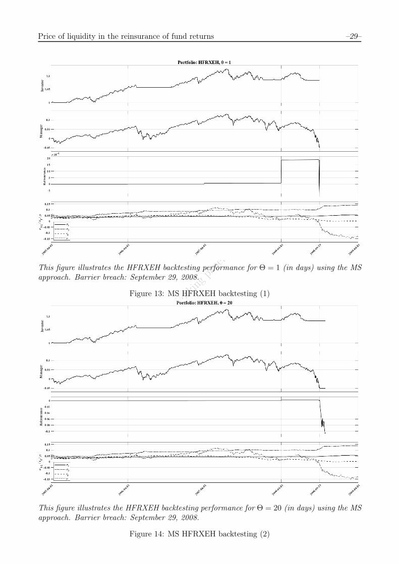
Figures 13 to 16 show results for the Markov-switching approach according to Chapter 4.

Figures 13 and 14 show roughly the same results for the HFRXEH Index as figures 7 and 8

(GBM approach) except that the amount of the premium is higher for the Markov-switching

approach. Figures 16 (MS) and 10 (GBM) yield similar results for the HFRXM Index. However,

the maximum value of the reinsurer in the Markov-switching model is more than twice as high

(VR ≈ 16 · 10−3 = 160bps), due to higher premiums.

Summing up the above: We obtain mixed results for both the geometric Brownian motion

and the Markov-switching approach. In some cases, losses can be absorbed by the paid pre-

mium. However, especially during the financial crisis, when sudden crashes caused funds to

suffer heavy losses, the premium was by far not high enough.

Working

pape

r


This figure illustrates the HFRXEH backtesting performance for Θ = 1 (in days) using theGBM approach. Barrier breach: September 29, 2008.

Figure 7: GBM HFRXEH backtesting (1)

This figure illustrates the HFRXEH backtesting performance for Θ = 20 (in days) using theGBM approach. Barrier breach: September 29, 2008.

Figure 8: GBM HFRXEH backtesting (2)

Working

pape

r


This figure illustrates the HFRXM backtesting performance for Θ = 1 (in days) using the GBMapproach. Barrier breach: January 28, 2010.

Figure 9: GBM HFRXM backtesting (1)

This figure illustrates the HFRXM backtesting performance for Θ = 20 (in days) using theGBM approach. Barrier breach: January 28, 2010.

Figure 10: GBM HFRXM backtesting (2)

Working

pape

r


This figure illustrates the HFRXGL backtesting performance for Θ = 20 (in days) using theGBM approach. No barrier breach occurred.

Figure 11: GBM HFRXGL backtesting

This figure illustrates the backtesting performance for an equally weighted (all HFRX indices)portfolio for Θ = 20 (in days) using the GBM approach. No barrier breach occurred.

Figure 12: GBM HFRX portfolio backtesting

Working

pape

r


This figure illustrates the HFRXEH backtesting performance for Θ = 1 (in days) using the MSapproach. Barrier breach: September 29, 2008.

Figure 13: MS HFRXEH backtesting (1)

This figure illustrates the HFRXEH backtesting performance for Θ = 20 (in days) using the MSapproach. Barrier breach: September 29, 2008.

Figure 14: MS HFRXEH backtesting (2)

Working

pape

r


This figure illustrates the HFRXM backtesting performance for Θ = 1 (in days) using the MSapproach. Barrier breach: January 28, 2010.

Figure 15: MS HFRXM backtesting (1)

This figure illustrates the HFRXM backtesting performance for Θ = 20 (in days) using the MSapproach. Barrier breach: January 28, 2010.

Figure 16: MS HFRXM backtesting (2)

Working

pape

r


7 Conclusion

We suggest an upfront premium to a reinsurance party in exchange for full portfolio protec-

tion, which goes beyond the insurance of the first tranche of losses by a first-loss scheme. The

additional downside protection extends the first tranche by considering a second one, that will

insure the investor against all losses, not just the first level. In this paper we propose both an

analytical closed-form solution based on a derivative-pricing approach with a geometric Brow-

nian motion as underlying framework and a numerical solution using a simulation based on a

Markov-switching model. In both approaches, we assume liquidity to be the key parameter and

thus, the premium is derived as a function of the underlying fund’s liquidity. A simplified back-

testing method delivers mixed results: for some hedge fund indices, historical losses especially

during the financial crisis were too high to be covered by the calculated premium. However, in

some cases the reinsurer was able to offset losses by collected premiums.

There are several extensions and questions that could be subject to future research. In

this paper, we suggest a total of two tranches. This framework could be extended, creating

a fund structure similar to an asset-backed security containing several tranches, each with a

different risk and return profile. The parameters could also be altered to a point where both

the reinsurance and the manager earn a fixed fee and a performance dependent fee. Finally,

the fund’s underlying liquidity is assumed to be homogeneous with daily liquidation steps

in our approach. Combining our approach with certain liquidation time distributions, e.g. an

exponential or Weibull distribution as suggested in Bordagand et al. (2014) and the optimization

of the liquidation process that comes along with the issue could be considered.

References

Baum, L., T. Petrie, G. Soules, and N. Weiss (1970). “A Maximization Technique Occurring

in the Statistical Analysis of Probabilistic Functions of Markov Chains”. The Annals of

Mathematical Statistics 41.1, pp. 164–171.

Bhaduri, R., B. Djerroud, F. Meng, D. Saunders, L. Seco, and M. Shakourifar (2018). “Fixed-

Income Returns from Hedge Funds with Negative Fee Structures: Valuation and Risk Analy-

sis”. In: Innovations in Insurance, Risk, and Asset Management. World Scientific Publishing,

pp. 217–238.

Bollen, N. (1998). “Valuing Options in Regime-Switching Models”. Journal of Derivatives 6,

pp. 38–50.

Working

pape

r


Bordagand, L., I. Yamshchikov, and D. Zhelezov (2014). “Portfolio Optimization in the Case

of an Asset with a given Liquidation Time Distribution”. arXiv preprint arXiv:1407.3154.

Chen, X., D. Saunders, and J. Chadam (2016). “Analysis of an Optimal Stopping Problem

Arising from Hedge Fund Investing”. Submitted to Journal of Mathematical Analysis and

Applications.

Djerroud, B., D. Saunders, L. Seco, and M. Shakourifar (2016). “Pricing Shared-Loss Hedge

Fund Fee Structures”. In: Innovations in Derivatives Markets. Springer, pp. 369–383.

Elliott, R., L. Chan, and T. Siu (2005). “Option Pricing and Esscher Transform under Regime

Switching”. Annals of Finance 1.4, pp. 423–432.

Elliott, R. and A. Swishchuk (2007). “Pricing Options and Variance Swaps in Markov-Modulated

Brownian Markets”. In: Hidden Markov Models in Finance. Springer, pp. 45–68.

Ernst, C., M. Grossmann, S. Höcht, S. Minden, M. Scherer, and R. Zagst (2009). “Portfolio

Selection under Changing Market Conditions”. International Journal of Financial Services

Management 4.1, pp. 48–63.

Escobar, M., V. Höhn, L. Seco, and R. Zagst (2017). “Optimal Fee Structures in Hedge Funds”.

Working paper, submitted for publication.

Hamilton, J. (1989). “A new Approach to the Economic Analysis of Nonstationary Time Series

and the Business Cycle”. Econometrica: Journal of the Econometric Society, pp. 357–384.

Hardy, M. (2001). “A Regime-Switching Model of Long-Term Stock Returns”. North American

Actuarial Journal 5.2, pp. 41–53.

He, X. and S. Kou (2018). “Profit Sharing in Hedge Funds”. Mathematical Finance 28.1, pp. 50–

81.

Henriksen, P. (2011). “Pricing Barrier Options by a Regime Switching Model”. Quantitative

Finance 11.8, pp. 1221–1231.

Höcht, S., K. Ng, J. Wiesent, and R. Zagst (2009). “Fit for Leverage-Modelling of Hedge Fund

Returns in View of Risk Management Purposes”. International Journal of Contemporary

Mathematical Sciences 4.19, pp. 895–916.

Hodder, J. and J. Jackwerth (2007). “Incentive Contracts and Hedge Fund Management”. Jour-

nal of Financial and Quantitative Analysis 42.4, pp. 811–826.

Kroese, D., T. Taimre, and Z. Botev (2013). Handbook of Monte Carlo Methods. John Wiley &

Sons.

Kwok, Y. (2008). Mathematical Models of Financial Derivatives. Springer.

Working

pape

r


Meng, F. and D. Saunders (2018). “Optimal Stopping and Variational Inequalities Arising from

Hedge Fund Fee Structures: Solutions and Asymptotic Analysis”. Working paper.

Merton, R. (1980). “On Estimating the Expected Return on the Market: An Exploratory In-

vestigation”. Journal of Financial Economics 8.4, pp. 323–361.

Saunders, D., L. Seco, C. Vogt, and R. Zagst (2013). “A Fund of Hedge Funds Under Regime

Switching”. The Journal of Alternative Investments 15.4, p. 8.

Viterbi, A. (1967). “Error Bounds for Convolutional Codes and an Asymptotically Optimum

Decoding Algorithm”. IEEE Transactions on Information Theory 13.2, pp. 260–269.

price of liquidity in the reinsurance of fund returns

Documents