price elasticities of key agricultural commodities …2 price elasticities of key agricultural...

1

Price Elasticities of Key Agricultural Commodities in China

Renan Zhuang and Philip Abbott1

July, 2005

Copyright 2005 by Renan Zhuang and Philip Abbott. All rights reserved. Readers may make verbatim copies of this document for non-commercial purposes by any means, provided that this copyright notice appears on all such copies.

1 Selected paper to be presented at the AAEA Annual Meeting, Providence Rhode Island, July 24-47, 2005. Zhuang is was Research Assistant and Abbott is Professor in the Department of Agricultural Economics, Purdue University, Krannert Building, 403 W State Street, West Lafayette, IN 47907-2056.Zhuang is now with Center for Agricultural Policy and Trade Studies, North Dakota State University, 209 Morrill Hall, Fargo, North Dakota 58105. Email addresses are [email protected] and [email protected].

2


Renan Zhuang and Philip Abbott

July, 2005

SHORT SUMMARY

We estimate a simultaneous equations model of Chinese markets for wheat, rice, corn,

pork, and poultry. Elasticities for consumption, feed demand, production, stocks demand, and

foreign trade fall within the range of results from previous studies, and are reasonable

magnitudes. China has market power in the trade for all commodities.

ABSTRACT We estimate a simultaneous equations model of Chinese agricultural markets which treats China

as a large trading country, and is built around supply-utilization tables for Chinese wheat, rice,

corn, pork, and poultry meat. Elasticities are estimated for consumption, feed demand,

production, stocks demand, and foreign demand or supply faced in China. While commodity

models are estimated using ITSUR in a single commodity simultaneous equations framework, an

LA/AIDS model of food demand is estimated using ITSUR as a system covering all

commodities. Results fall within the wide range of results from previous studies, and are quite

reasonable magnitudes. China has market power in the trade for all five commodities under

study.

3


INTRODUCTION

Both market events of the mid-1990s and China’s entry into the WTO have sparked a

lively debate on the future role of China in agricultural markets. Widely divergent opinions on

whether China would emerge as a significant grain or meat importer have been voiced, based on

forecasts by USDA, IFPRI, the Chinese government, and many others (Carter and Rozelle; Han

and Hertel). Lester Brown’s projections in 1995 suggested China could need imports close to the

current volume of international grain trade (200-370 million metric tons). Western influenced

forecasts (Rozelle et al 1996; Huang 1998; Wang et al 1998; Geng et al 1998; ERS, USDA 1997,

2002, and 2004 ) have been much lower, and highly variable, both across forecasters and over

time, but tend to suggest grain imports by China could reach 20-40 million metric tons in the

next decade. Chinese government forecasts (Song 1997, Lin 1998, IOSC 1996) have indicated

China would remain relatively self-sufficient. Market outcomes since 1995 have been more

consistent with the Chinese forecasts, in spite of Chinese entry into the WTO in 2002.

While some of the differences in forecasts stem from differences in assumptions on

future Chinese production, population and income growth, differences in estimated and assumed

supply and demand elasticities, and treatment of price effects (or lack thereof) on trade, also help

account for these widely divergent projections. Better understanding of Chinese commodity

markets, and specifically better estimates of supply and demand elasticties, would permit

construction of better models to predict trade flows, to analyze agricultural policies, and to test

hypotheses on the structure and performance of those markets.

4

One particular problem is that China may be a large country in world agricultural markets

(Carter and Schmitz, 1979), yet virtually all studies treat China as a small country (e.g. Chern et

al 1999, Mitchell and Ingco 1993). If China is a large country in international markets, not only

must simultaneous equation methods be used to estimate supply and demand parameters, but also

assessment of Chinese policy must take into account this potential market power in trade. For

example, Chinese restriction of imports following the 1995 world grain price increases may be

explained within an optimal tariff framework. Chinese limitations on imports may have helped to

keep world prices lower than they would have otherwise been after 1996, reducing Chinese

import costs. Hence, self-sufficiency may be defended not only on political economy grounds,

but also for reasons of trade policy efficacy. To analyze this, we must know better the relevant

domestic and trade elasticities for the Chinese market.

In this study we estimate a simultaneous equations model of Chinese agricultural markets

which treats China as a large trading country. The model structure is built around China’s

supply-utilization tables for Chinese grains and meats. Elasticities are estimated for domestic

consumption, feed demand, domestic production, stocks demand, and foreign demand or supply

faced in China. Chinese behavior in foreign markets may then be derived from the domestic

market parameters and trade policy assumptions.

The commodities under study include wheat, rice, corn, pork, and poultry meat. China’s

domestically produced wheat, rice, and corn and the corresponding foreign commodity

(regardless of origin) are assumed to be homogenous goods or perfect substitutes. While

imported pork and poultry meat are assumed to be differentiated from China’s domestically

produced pork and poultry meat, China’s exported pork and poultry meat are assumed to be

similar to its domestically produced goods.

5

An LA/AIDS model is used to estimate consumption covering all commodities as a sub-

system, so that constraints from demand theory may be imposed in estimation. Variables for

household income, per capita consumption, and prices are all at the national level, and are

estimated using time series data. Previous studies have used either rural or urban household

survey data or household survey data from a province covering a period of 2 to 5 years (Lewis

and Andrews; He and Tian).

Supply and feed demand equations are specified within a profit maximization structure

for farms. A single commodity simultaneous equations model is then estimated as another sub-

system (hereinafter refers to as the supply sub-system) for all equations except for food

consumption.

Instrumental variables estimation methods are used to correct for simultaneity bias in the

demand sub-system and in each commodity sub-system. Potential instrumental variables are the

exogenous variables that appear in the whole system of supply and demand equations. ITSUR is

used to correct for cross equation error correlation in both the LA/AIDS sub-system and the

supply sub-system for each commodity model.

MODELS AND ESTIMATION METHOD

In this study it is assumed that there are two regions in the world, China and the rest of

the world (ROW). Substantial two way trade is observed for poultry meat, and must be

accounted for in estimating a trade model. A CES nest of demand for poultry meat is used to

help explain the substantial two-way trade observed in China. While there is now also two way

trade in pork, no CES nest will be estimated since there were virtually no observations for pork

imports prior to 1998, and the imports afterwards are very small relative to China’s domestic

6

demand. Thus, the imported pork is treated as a substitute for China’s domestic pork

consumption. Exports of both pork and poultry meat are assumed homogenous substitutes for

the domestic goods.

While supply sub-system is estimated in a single commodity simultaneous equations

model, an LA/AIDS model with a CES nest for poultry meat is estimated as a food demand sub-

system covering all commodities. Figure 1 depicts our LA/AIDS model with a CES nest for

poultry meat.

Utility (LA/AIDS)

Figure 1: LA/AIDS Model with a CES Nest for Poultry Meat

What follows is a discussion of the LA/AIDS model for the estimation of food demand

sub-system equations and the single commodity simultaneous equations model for the estimation

of supply sub-system of all other equations.

Model Specification for Estimation of Food Demand Elasticities

The Almost Ideal Demand System (AIDS) of Deaton and Muellbauer (1980) is one of the

most widely used flexible demand system specifications. It gives an arbitrary first order

Wheat Rice Corn Pork Poultry (CES)

Domestic Imported

Other

7

approximation to any demand system and satisfies the axioms of choices exactly. It aggregates

perfectly over consumers and has a functional form that is consistent with known household-

budget data. The AIDS demand functions in budget share form is as follows:

∑=

⎟⎠⎞

⎜⎝⎛++=

n

jijijii P

Ypw

1

lnln βγα (1)

Where iw is the budget share for good i, and Y is the total expenditure or income, and lnP is a

price index defined by ∑ ∑∑= ==

++=n

k

n

jjkkj

n

kkk pppP

1 110 lnln

2

1lnln γαα .

Because the AIDS model constitutes a non-linear system of equations, and it is tedious to

estimate the constant term in the price index, many previous studies (Deaton and Muellbauer

1980, Alston et al 1994, Halbrendt et al 1994) have used ∑=

=n

kkk pwP

1

* lnln (Stone’s price

index) instead of lnP. The model that uses Stone’s index is called the “linear approximate AIDS”

or LA/AIDS model. If prices are highly collinear, P may be well approximated as proportional to

P*, i.e. PP φ≅* , and the LA/AIDS model is a good approximation to the AIDS model.

Empirically, LA/AIDS is often used in the existing literature to estimate China’s agricultural

commodity demand functions (e.g. Lewis et al 1989, Cai et al 1998, Liu et al 2001, Wu et al

1995).

After incorporating dummy variables and other demographic variables, the LA/AIDS

model looks as follows:

∑=

⎟⎠⎞

⎜⎝⎛++=

n

jijijii P

Mpw

1*

* lnln βγα + ∑=

m

kkik D

1

λ + iε (2)

Where φβαα ln*iii −= , ∑

=

=n

kkk pwP

1

* lnln , sDk ' (k = 1, 2, …m) are dummy and/or

8

demographic variables, sik 'λ are parameters to be estimated, and iε is the error term associated

with equation i. In this study, kD ’s include an urbanization index and two dummy variables that

capture the effects of the rationing system. SinceiIn 1993, China further liberalized the grain

market and abolished the 40-year old grain rationing system (Fan and Cohen, 1999).

For the LA/AIDS model to be consistent with consumer theory, the parameters in the

demand system must satisfy the following restrictions:

11

* =∑=

n

iiα 0

1

=∑=

n

iiβ 0

1

=∑=

n

iijγ (Adding up)

01

=∑=

n

jijγ (Homogeneity)

jiij γγ = (Symmetry)

The income and price elasticities derived based on this model are:

i

ii w

βη += 1 (Expenditure or income elasticity)

[ ] [ ] IIAIBCE −++= −1 (Price elasticities in matrix form)

Where i

ji

i

ijijij w

w

wa β

γδ −+−= in A (a nn × matrix, here n = 6), and ijδ =1 if i =j, ijδ = 0 if i≠ j;

i

ii w

bβ

= in B (a 1×n vector); jjj Pwc ln= in C (a n×1 vector) (Green and Alston, 1990).

As depicted in the above Figure 1, per capita household income is assumed to be spent on

six commodities, namely, wheat, rice, corn, pork, poultry meat, and other goods. Commodity

‘Other’ represents all other goods aggregated, excluding pork, poultry, wheat, rice, and corn.

This ‘Other’ good is included so that all income (expenditure) is exhausted. Note that poultry

9

meat in the LA/AIDS layer is an aggregated good in the sense that it includes differentiated

imported and domestically produced poultry meat, respectively.

The CES utility function for poultry meat is as follows:

U = 11

2

1

1 )1(−−−

⎟⎟⎠

⎞⎜⎜⎝

⎛−+

σσ

σσ

σσ

αα XX (3)

Where 1X is the quantity of domestic poultry meat consumed and 2X is imported poultry meat

consumed, α and (1-α ) are the share parameters and σ is the constant elasticity of substitution

between the two goods. Note that 0< α <1 and σ >0.

Maximizing (1) subject to the budget constraint C = P1X1 + P2X2 results in the following

demand functions:

iX = σα ( )Xσ−

⎟⎠⎞

⎜⎝⎛

P

P1 i = 1, 2 (4)

Where P = ⎟⎟⎠

⎞⎜⎜⎝

⎛++

21

2211

XX

XPXP is the weighted average price and X is aggregate demand (i.e. X =

X1 +X2) from the LA/AIDS model. Note that C = PX.

Taking the natural logarithm form of (4), we get:

ln iX = σ lnα + ln X - σ (ln iP -LnP) i =1, 2 (5)

Note thatσ lnα and σ ln(1-α ) are constants since both α and σ are constant parameters.

Thus, equation (5) can be readily used in regression to determine the magnitude ofσ .

Model Specification for Estimation of Other Elasticities

Other elasticities to be estimated include China’s domestic supply, feed demand, stocks

demand, and foreign import demand (or export supply) elasticities. The following single

10

commodity simultaneous equations model is used for estimation of these other elasticities:

),( sd

ss ZpQQ = (6)

),( dd

dd ZpQQ = (7)

),( feedd

feedfeed ZpQQ = (8)

),( std

stst ZpQQ = (9)

mQ = dQ + feedQ + stQ - sQ - 1−stQ (10)

),( xf

xf

ww ZQpp = (11)

mQ = xfQ (12)

tpp wd += (13)

Equation (6) is China’s domestic supply function. It is a function of domestic

price dp and a vector of supply shifters sZ . The potential supply shifters include labor input, land

input, fertilizer input, pesticides input, and capital.

Equation (7) is China’s domestic demand function. It is a function of domestic

price dp and a vector of demand shifters dZ . The potential demand shifters include income and

population. Note that demand functions are estimated using the LA/AIDS model. The food

demand equation is included here to identify other equations.

Equation (8) is China’s domestic feed demand equation. It is a function of China’s

domestic price dp and a vector of feed demand shifters feedZ . The potential feed demand shifters

include production of pork and poultry. For corn, feed demand is estimated using the pork

model, while this equation is directly estimated for wheat.

Equation (9) is China’s domestic stocks demand function. It is a function of domestic

consumer price dp and a vector of stock shifters stZ . The potential stock shifters include

beginning stocks and production.

11

Equation (10) is an identity yielding China’s import demand (or export supply if mQ < 0).

It simply states that China’s net import demand equals to China’s excess demand ( dQ + feedQ -

sQ ) plus the change of its stocks ( tstQ - 1−t

stQ ). Equation (10) implies that all shifters sZ , dZ , feedZ ,

and stZ would affect China’s import demand through equations (6), (7), (8), and (9).

Equation (11) is the foreign inverse export supply (or inverse import demand if xfQ < 0)

function. It represents the behavior of ROW. It is assumed that the world price faced by

China wp is a function of foreign exports xfQ (to China) and a vector of foreign export

shifters xfZ . The potential foreign export shifters include foreign production and beginning

stocks. This equation is estimated in the inverse form so that hypotheses on Chinese market

power in trade can be formally tested.

Equation (12) is an identity, which states that China’s net import demand or export

supply is equal to foreign net export supply or import demand. This condition implies that the

world markets for wheat, rice, corn, pork, and poultry meat clear at the Chinese border. Equation

(13) is another identity, which states that China’s domestic price dp equals to world price wp

plus the equivalent specific tariff imposed on imported good.

While a simultaneous equations model has been used in previous studies to estimate

China’s agricultural commodity supply function (e.g. Seale 1999, Wang 2000), they only look at

the supply side and ignore the demand side. Simultaneity problems could arise in that case.

Moreover, the specifications of each equation in their simultaneous equation system do not

follow strictly production theory.

In this study, producers are assumed to behave as profit maximizers and price takers.

Thus, a neo-classical economic profit maximization approach will be used to

12

derive a supply specification for each commodity under study. That is, producers

Max Π(p, w) = py – r’x subject to (y,x) ∈ Ω

Where y is output, p is the output price, x is a vector of inputs, r is a vector of input prices, and Ω

represents technology. Suppose the profit function is well defined, and its first derivatives exist

everywhere. Then, according to Hotelling’s lemma, the supply function is p

rp

∂Π∂ ),(

= S(p, r).

It is assumed that producers have full information about the prices and their expectations

about prices are rational and are assumed to be realized. In other words, all the prices

determining supply are current prices rather than lagged prices. The reasons behind this include:

a) We are using procurement prices as proxy variables for China’s domestic producer and

consumer prices. b) The procurement prices and farm input prices are in fact set by the Chinese

government and are typically announced in advance (before sowing and planting). c) While the

Chinese government has adjusted its procurement prices and farm input prices over time,

farmers’ expectations for prices do not vary much from the officially promulgated prices for a

specific year.

A Cobb-Douglas production function is assumed for the technology. However, since data

on input quantities such as labor, fertilizers, and pesticide are not available by crop, the following

Cobb-Douglas restricted profit function is often used empirically to derive output supply and

input demand functions (Lau and Yotopoulos 1971, 1972).

Zrp ii

i lnlnlnln 10 γβααπ +++= ∑ (14)

Where π is the profit, p is the output price, ir is the price of input i, (i = labor, fertilizers,

pesticides, capital), and Z is the fixed input of land (i.e. cultivated acreage) in use for the crop

under study.

13

Homogeneity of degree one in prices for the profit function implies that 1α =1-∑i

iβ . By

(14), taking partial differentiation with respect to pln and irln , respectively, we get,

pln

ln

∂∂ π

=π

π p

p∂∂

=1-∑i

iβ and

irln

ln

∂∂ π

=π

π i

i

r

r∂∂

= iβ

By Hotellings Lemma, ),( rpQp s=

∂∂π

and ),( rpXr i

i

−=∂∂π

. Thus, the output supply function is

),( rpQs = (1-∑i

iβ ) p

π

Hence, ln ),( rpQs = ln(1-∑i

iβ ) + lnπ - ln p

Taking partial differentiation with respect to pln , we get

p

Qs

ln

ln

∂∂

= pln

ln

∂∂ π

- p

p

ln

ln

∂∂

= -∑i

iβ

Thus, the own price elasticity of output supply function is -∑i

iβ , where iβ are the parameters to

be estimated in the Cobb-Douglas restricted profit function (14).

Similarly, the factor demand function for each i is,

),( rpX i = - iβir

π

Hence, ln ),( rpX i = ln(- iβ ) + πln - irln

Taking partial differentiation with respect to irln , we get

i

i

r

X

ln

ln

∂∂

= irln

ln

∂∂ π

- i

i

r

r

ln

ln

∂∂

= iβ - 1.

14

Thus, the own price demand elasticity for factor i is iβ - 1. Note that corn feed is used as a proxy

variable for feed input in pork production in China. Formula iβ - 1 (i = corn) will give us the feed

demand elasticity for corn in China.

The following illustrates the specific commodity model to be estimated for the case of

wheat:

πln = a0+a1lnPd + a2lnWage + a3lnPfert + a4lnPpesti + a5lnP1tool

+ a6lnPoil +a7lnA + a8year ------ Cobb-Douglas restricted profit function

sQ = (1- a2 - a2 – a4- a5 – a6 )dP

π ------ Wheat output supply

dQ = b0 + b1 dP + b2Pop + b3M + b4urban ------ Food demand equation

feedQ = c0 + c1Pd + c2QSpk + c3QSpy ------ Feed demand equation

stQ = d0+d1Pd +d2 sQ ------ Stocks demand equation

mQ = dQ + feedQ + stQ - sQ - 1−stQ ------ China’s import demand

wp = e0 + e1 xfQ + e2BSfp+e3Qsfp+e4Rer ------ Inverse foreign export supply

mQ = xfQ ------ World market clearing condition

tepp wd += ------ Price linkage

Note that food demand equation will not be estimated here (it is estimated in the

LA/AIDS model). It is included to identify other functions in the system. A is planted acreage

for wheat, and Wage is farmers’ annual wage. Pop, M, and urban represent China’s population,

household income, and urbanization index, respectively. Pfert, Ppesti, P1tool, and Poil are prices for

fertilizers, pesticides, small farm tools, and farm machinery oil, respectively. All prices are in

real terms and are deflated by China’s national CPI. Year is a trending variable. QSpk and QSpy

15

represent China’s pork and poultry meat production, respectively. BSfp and Qsfp represent the

ROW’s per capita beginning stocks and per capita production, respectively. Rer and e are the

real exchange rate and nominal exchange rate in Chinese Yuan per US dollar.

The expected sign for a2 is negative since a higher wage means higher labor cost for the

production. The expected signs for a3, a4, a5, and a6 are negative. This is straightforward since an

input demand function typically slopes downward. The expected sign for a7 is positive since

higher planted acreage leads to higher production, ceteris paribus. The expected sign for a8 is

positive since the production of wheat trends upward over the time. The expected sign for c1 is

negative since a demand function slopes downward. The expected signs for c2 and c3 are

positive since higher production of pork and poultry lead to higher demand for feed. The

expected sign for d1 is negative since people tend to sell more and hold lower stocks when the

market price is high. The expected sign for d2 is positive since higher production leads to higher

stocks, ceteris paribus. The expected sign for e1 is positive since the higher the world price, the

more the foreign exporter tends to supply. The expected signs for both e2 and e3 are positive

since higher per capita foreign beginning stocks and production induce the foreign country to

export more, ceteris paribus. The expected sign for e4 is negative since a higher real exchange

rate implies devaluation of Chinese Yuan, which leads to lower imports into China.

The above commodity model is used with minor modifications for the cases of rice, corn,

pork, and poultry meat. The feed demand equation will be ignored in the case of rice (since there

is no statistics for feed use of rice). The stocks demand equations will be ignored in the cases of

pork and poultry meat since there are no statistics for stocks. Also, two-way trade is taken into

consideration in the case of poultry meat. That is, there are two foreign behavioral equations.

One is inverse foreign export supply function, and the other is an inverse foreign import demand

16

function. Corn is used as a factor input in pork production, and the expected sign for a factor

input is negative.

Data

Time series data are obtained from various database sources, including FAOSTAT,

USDA PS&D and various issues of China Statistical Yearbook. The data covers a period of 24

years from 1978 to 2001. Production, consumption, stocks, and feed demand data for wheat, rice,

corn, and pork are obtained from the USDA PS&D database2. For poultry meat, USDA PS&D

does not report China’s poultry production until 1987. Moreover, data from PS&D and

FAOSTAT databases do no match each other. Data from FAOSTAT are used here.

Border prices of all commodities under study are unit value obtained from the FAOSTAT

database. China’s domestic prices are producer prices. Domestic prices of wheat, rice, and corn

in 1991 -2001 are obtained from the FAOSTAT database, and those for the other years are

estimated using a regression method based on the purchasing price indices in 1978 -2001 from

China Statistical Yearbook. Domestic prices for poultry meat and pork for 1991 – 2001 are

obtained from the FAOSTAT database. Domestic prices for pork in 1978 – 1990 and domestic

prices for poultry meat in1978 - 1987 are obtained from various issues of China Statistical

Yearbook. Domestic prices of poultry meat for 1988-1990 are estimated using extrapolation. All

other variables including wages, price indices of fertilizers, pesticides, and farm tools are

obtained from various issues of China Statistical Yearbook. All prices are deflated by China

national CPI obtained from various issues of China Statistical Yearbook.

2 The data from the USDA PS&D and FAOSTAT databases are essentially the same for these commodities.

17

Estimation Method

Two-stage least squares (2SLS) or instrumental variables estimation has been widely

used to address the simultaneity problem in trade models since the late 1970s. Regardless of the

number of equations in a simultaneous equations model, each identified equation can be

estimated by 2SLS. The instruments for a particular endogenous variable consist of the

exogenous variables appearing anywhere else in the system. However, when a system with more

than two equations is correctly specified, system estimation methods such as 3SLS are generally

more efficient than estimating each equation by 2SLS. This is because 2SLS estimator does not

take into account the cross-equation correlation of the errors.

The most commonly used system estimation method in the context of simultaneous

equations model is three stage least squares (3SLS). The 2SLS estimates are used to estimate the

error covariance matrix for the system of equations required for 3SLS. The 3SLS estimator is

computed by applying the GLS-SUR (generalized least squares and seemingly unrelated

regression) transformation to the simultaneous equation model.

In this research, demand equations and supply equations are estimated separately, as

discussed earlier. 3SLS estimation method cannot be used directly in this case. Equivalently,

instrumental variables estimation will be used to address the simultaneity problem while the

iterative seemingly unrelated regression (ITSUR) method will be used to take into account the

cross-equation correlations within the two sub-systems estimated in the study. The instrumental

variables are virtually the exogenous variables that appear in the whole system of supply and

demand equations.

The supply and demand framework approach has been widely used for predicting future

trade of agricultural commodities. All other long term models are more or less patterned after

18

USDA or FAPRI baseline models (Baumel, 2001), which utilizes the supply and demand

framework approach. A country’s domestic supply and demand for a commodity are typically

estimated separately, and the difference between supply and demand is taken to obtain the excess

supply or excess demand for the commodity. For this study, if we estimate systematically the

whole supply and demand equations system for all the five commodities under study, there

would involve more than 22 equations. Since we have only 24 observations for the supply sub-

system and 20 observations for the food demand sub-system (there were no statistics for China’s

imports of poultry meat until 1982), it does not allow us to estimate the whole system at one

time. Therefore, like previous studies, we also estimate the supply (supply sub-system) and

demand (food demand sub-system) separately.

We believe that cross equation error correlations are most likely within food demand,

since that is a behavioral representation for consumers, and then across equations of a single

commodity system, capturing within market effects, as modeled here. A much more cumbersome

estimation approach would have been required to capture less likely cross commodity error

correlations in relationships other than food demand.

ESTIMATION RESULTS AND DISCUSSION

First, estimation results for the LA/AIDS model of food demand are discussed. Second,

estimation results for each single commodity simultaneous equations model are presented.

Finally, our estimated elasticites are compared to those reported in the previous studies

19

Food Demand Elasticities in China

The estimation results for the LA/AIDS model using mean prices to convert estimated

parameters to elasticity form are summarized in Table 1. Parameter estimation results including t

statistics and p-values are summarized in Table 2.

As shown in Table 1, all the own price elasticities have expected negative signs and all

income elasticities have expected positive signs. The mean price elasticities of demand for

wheat, rice, corn, pork, and poultry meat are -0.298, -0.352, -0.477, -0.266, and – 0.438,

respectively. While the own price elasticities for all three goods are inelastic, the elasticity for

corn is relatively high. The income elasticities of demand for wheat, rice, corn, pork, and poultry

meat are about 0.519, 0.136, 0.852, 0.01, and 0.78, respectively.

The demand elasticity for poultry meat is the aggregate demand elasticity because of the

CES nest used for poultry meat. That is, poultry meat consumed in the LA/AIDS model

aggregates both China’s domestically produced poultry meat and imported poultry meat. The

CES nest is estimated to determine the elasticity of substitution between domestic and imported

poultry meat.

Before estimating the CES nest, the estimated prices for domestically produced and

imported poultry meat are obtained by regression of observed prices on the instrumental

variables, respectively. The instrumental variables are the same as those used in the estimation of

the LA/AIDS model. Using the ITSUR estimation method, the estimation results for the CES

nest are summarized in Table 3:

The constant elasticity of substitution between China’s domestically produced poultry

and imported poultry is σ = 0.810 and is statistically significant at 10% alpha level. By (5)

iiε = ptiaaεε - σ + σ ptiε i = 1, 2 (15)

20

Where 11ε and 22ε are own price demand elasticities for X1 and X2, respectively. aaε is

demand elasticity for the aggregated poultry commodity obtained from the LA/AIDS model;

1ptε and 2ptε relate the responsiveness of aggregated price to the change of domestic price and

imported price, respectively; And σ is the constant elasticity of substitution between domestic

and imported poultry.

It can be shown that

iiε = σε

σε+− aai

aai

a

a

)1( i = 1, 2 (16)

Where 1a and 2a are the estimated parameters for lnX that appear in (5).

Plugging aaε = 0.4383, σ = 0.810, a1 = 0.9809, and b1 = 3.0863 into (16), we get the price

demand elasticity for domestically produced poultry meat 11ε = 0.434, and China’s import

demand elasticity for poultry meat 22ε = 0.636. The elasticities for both domestic and imported

poultry meat are inelastic.

The above results imply that poultry meat is relatively more a “luxury” good (note that

both poultry meat and pork are not luxury goods because of inelastic demand elasticities) as

compared to pork for two reasons: first, the demand elasticity for poultry meat is higher than that

for pork. Second, the substitution elasticity between domestic and imported poultry meat is low.

In fact, most of the modern poultry factories are located in the suburbs of big cities and the

poultry products are primarily sold to urban residents who have higher income than rural

residents.

21

China’s Supply, Stocks Demand, Feed Demand, and Trade Elasticities

This section presents the estimation results for the supply sub-system for wheat, rice,

corn, pork, and poultry meat, respectively. As discussed earlier, the supply sub-system for each

commodity under study is estimated using a single commodity simultaneous equations model.

Wheat

The estimation results for wheat are summarized in Table 3. All the estimated

parameters except a2, a3, c2 and e3 have expected signs. China’s supply elasticity is –(a2+ a3+a4 +

a5 + a6 ) = 0.311. The slope of feed demand equation c1 = -0.01567 has the expected negative

sign and is statistically significant at a 5% alpha level. The corresponding mean price elasticity is

about -1.493 using mean price and mean quantity for 1978 – 2001. The slope of the stocks

demand equation d1 = -0.20398 has expected negative sign and is statistically significant at a 1%

alpha level. The corresponding mean price elasticity is about -1.214. The slope of inverse foreign

export supply equation e1 = 3.664 has expected positive sign and is statistically significant at a

1% alpha level. The corresponding mean price elasticity is about 3.183.

Does China have market power in wheat trade? A one-tail t test at a predetermined 5%

significance level is conducted to test this hypothesis. The calculated t is 2.850 as shown in Table

3, which is greater than the critical t value, 23,05.0t = 1.714. Thus, we reject the null hypothesis.

We are 95% confident that the slope of foreign export supply of wheat is strictly greater than

zero. This implies that China has market power in wheat trade.

Rice

The estimation results for rice are summarized in Table 4. All the estimated parameters

except a2, a4, a7, and e4 have expected signs. China’s domestic output supply elasticity is –(a2+

a3+a4 + a5 + a6 ) = 0.273. The slope of stocks demand equation, d1 = -0.2422, has the expected

22

negative sign. The corresponding mean price elasticity is -1.102. The slope of the inverse

foreign import demand equation, e1 = -23.43 has the expected negative sign and is statistically

significant at a 5% alpha level. Thus, we are 95% confident that China has market power in rice

trade. The corresponding mean price elasticity is about -8.240.

Corn

As discussed earlier, feed demand for corn is derived from pork producer’s profit

maximization problem. The estimation results for corn are summarized in Table 5. All the

estimated key parameters have expected signs. The output supply elasticity is about 0.230. The

slope of the stocks demand equation d1 = -0.1924 has expected negative sign and is statistically

significant at a 10% alpha level. The corresponding mean price elasticity is about -0.612. The

slope of the inverse foreign import demand equation e1 = -5.120 has expected negative sign and

is statistically significant at a 1% alpha level. This implies that China has market power on corn

trade. The corresponding mean price elasticity of foreign import demand is about -3.781. The

elasticity of feed demand for corn is -0.761 (from the pork model).

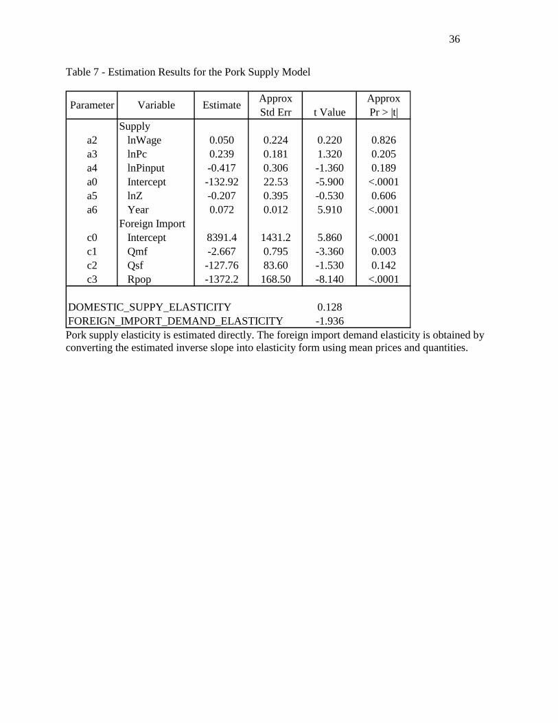
Pork

The estimation results for pork are summarized in Table 6. While not all the estimated

parameters have the expected signs, all the key parameters have expected signs. The elasticity for

China’s domestic production function is -(a2+a3+a4) = 0.128. The slope for the inverse foreign

import demand function is c1 = -2.667 and is statistically significant at 1% alpha level. This

indicates that China has market power in its pork exports. The corresponding mean price

elasticity for the foreign import demand curve is about -1.936. The own price factor demand

elasticity for corn is (a3 – 1) = -0.761.

23

China’s domestic supply response to pork price is quite low. If the domestic pork price

increases by 1%, the domestic supply will increase by only 0.13%. The foreign import demand

elasticity that China faces is elastic.

Poultry

The estimation results for poultry meat are summarized in Table 7. While not all the

estimated parameters have the expected signs, all the key parameters have expected signs. The

elasticity for China’s domestic production function is -(a2+a3) = 0.306. The slope for the inverse

foreign import demand function is b1 = -0.593 and is statistically significant at a 1% alpha level.

This implies that China has market power in its exports of poultry meat. The slope for inverse

foreign export supply function is c1 = 0.694 and is statistically significant at a 5% alpha level.

This suggests that China has market power in its imports of differentiated foreign poultry meat,

as well. The corresponding mean price foreign import demand and foreign export supply

elasticities are about -8.440 and 2.566, respectively.

We have also estimated the above models for each commodity with foreign export supply

and/or foreign import demand equations specified ordinarily (i.e. Q = Q(p, Z)). Key estimation

results for each commodity model estimated in ordinary form are summarized in Table 9. For

wheat, foreign export supply elasticity becomes inelastic (0.785). For pork, foreign import

demand elasticity becomes inelastic as well (-0.751). For poultry meat, foreign export supply

elasticity becomes inelastic (0.668).

It is clear that foreign import demand or export supply elasticity tends to be more elastic

when foreign behavior equation is specified inversely in each commodity model.

24

Moreover, the inverse specification not only allows directly testing for market power, but also

yields greater statistical significance (or lower standard errors) on the trade elasticities. Other

parameters change only slightly with variation in specific demand.

Our Estimates versus the Estimates in Previous Studies

This section compares our estimated elasticities to those reported in previous studies. The

elasticities for grain commodities are discussed first, and then the elasticities for meat products

are explored.

Grain

Rozelle and Huang (2000) estimated that the short-run output supply elasticities for

wheat and corn in China were 0.049 and 0.343, respectively, and the long-run output supply

elasticities were 0.043 and 0.289, respectively. Our estimated output supply elasticities as shown

in Table 9 are 0.311, 0.273, and 0.230 for wheat, rice, and corn, respectively. These estimates are

very close to the estimate by Rozelle and Huang in the case for corn, and their wheat elasticities

are very low.

Huang and Rozelle (1995) estimated that the own price elasticity for grain in China was -

0.52 and income elasticity for grain was 0.86. Hus et al (2002) estimated that the own price

elasticity of demand for grain was -0.16 and – 0.37 for China’s urban consumers and China’s

rural consumers, respectively. Their estimates for income elasticities for urban and rural

consumers were 0.11 and 0.32, respectively. Halbrendt et al (1994) estimated that the own price

demand elasticity and for grain in Guangdong Province, China was -0.233, and the expenditure

elasticity for grain was 0.575. Liu and Chern (2001) used different models to estimated food

consumption in China’s Jiangsu Province. Their estimates for the own price elasticity for rice

25

ranged from -0.894 to – 1.203. And their expenditure elasticities for rice ranged from 1.107 to

1.345. Gao et al (1996) also estimated food demand using data for Jiangsu Province. Their

estimated own price elasticity for grain was -0.988, and the expenditure elasticity was 0.516.

As shown in Table 9, our estimated own price demand elasticity for wheat, rice, and corn

are -0.298, -0.352, and – 0.476, respectively. And our estimated income elasticities for wheat,

rice, and corn are 0.519, 0.136, and 0.852, respectively. It is clear that our estimated elasticities

fall within the wide ranges of elasticity estimates in these previous studies.

Meat

Pudney and Wang (1991) estimated that the own price elasticities of demand for pork and

poultry in China were -0.04 and -0.005, respectively. Their estimated income elasticities for pork

and poultry were 0.923 and 0.716, respectively.

Hsu et al (2002) estimated that the own price demand elasticities for pork and poultry for

urban residents were -1.59 and -1.28, respectively, and those for rural residents were -0.66 and -

0.50, respectively. Their estimated income elasticities for pork and poultry for urban residents

were 1.68 and 3.12, respectively, and those for rural residents were 0.67 and 0.70, respectively.

He and Tian (2000) reported that many other studies have estimated own price elasticities

of demand for pork and poultry in China were within the above range. That is, own price demand

elasticity for pork fell between -0.04 and -1.59. And the own price elasticity for poultry fell

between -0.005 and -1.28. As shown earlier, our estimated demand elasticities for pork and

poultry meat were about -0.27 and -0.44, respectively, which also fell in the range for elasticity

estimates of previous studies.

26

CONCLUSION

Estimated elasticities for wheat, rice, corn, pork, and poultry meat are summarized in

Table 8. These results fall within the wide range of results from prior studies, and are quite

reasonable magnitudes relative to those earlier results. Foreign import demand or export supply

elasticity tends to be more elastic and more significant statistically when the foreign behavioral

equation is specified inversely in each commodity model. That specification also allows us to

directly test the hypothesis on China’s market power in trade, a motivating concern in this paper.

Previous studies showed that the own price demand elasticity for grain in China ranged

from -0.16 to -1.203. While China’s pork demand elasticity ranged from -0.04 to -1.59, its

poultry meat demand elasticity ranged from -0.005 to -1.28. Our estimated own price demand

elasticities for wheat, rice, corn, pork, and poultry meat are -0.298, -0.352, -0.476, -0.27, and -

0.44, respectively. While our estimated income elasticities for wheat, rice, corn, and poultry meat

fall within the range of estimated income (or expenditure) elaticities in previous studies, our

estimated income elasticity for pork is only 0.01, which is extremely low. Other income

elasticities are at more reasonable levels.

Trade elasticities faced by China range from 3.183 to -8.440, and are significantly

different from what would be expected for a small trader. The estimation results show that

China has market power in the trade for all five commodities under study. Hence, the approach

taken in this study is needed both for estimation and for subsequent policy analysis.

27

REFERENCES Alston J. M., K. A. Foster, and R. D. Green. “Estimating Elasticities with the Linear

Approximate Almost Ideal Demand System: Some Monte Carlo Results”, The Review of Economics and Statistics 76 (1994): 351 -356.

Brown, L. R. Who Will Feed China? The Worldwatch Environmental Alert Series,

W.W. Norton & Company, 1995.

Baumel, C.P. “How U.S. Grain Export Projections from Large Scale Agricultural Sector Models Compare with Reality”, May 15, 2001. www.iatp.org/enviroObs/library/uploadedfiles/How_US_Grain_Export_Projections_from_Large_Sca.pdf

Cai H.O., Brown, C., Wan, G. H., and J. Longworth. “Income Strata and Meat Demand

in Urban China”, 1998. http://www.agribusiness.asn.au/review/1998v6/chinameat.htm

Carter, C., and S. Rozelle. “Will China Become a Major Force in World Food Markets?” Review of Agricultural Economics 23(2001): 319-331.

Carter, C., and A. Schmitz. “Import Tariffs and Price Formation in the World Wheat

Market”, American Journal of Agricultural Economics 61(1979):517-522. Chern, W. S. and S. Yu, “Econometric Analysis of China’s Agricultural Trade Behavior”,

Feb. 1999, http://www.china.wsu.edu/pubs/pdf-98/chern-6.pdf Deaton A., and J. Muellbauer. “An Almost Ideal Demand System”, American Economic

Review 70 (1980): 312-326. ERS/USDA, “International Agriculture Baseline Projections to 2005”, Agricultural

Economic Report No.750, 1997. ERS/USDA, “Agricultural Baseline Projections: baseline presentation, 2002-2011”,

March 11, 2002, http://www.ers.usda./gov/briefing/baseline/present2002.htm ERS/USDA, “USDA Agricultural Baseline Projections to 2013”, Staff Report WAOB-

2004-1, February 2004, http://www.ers.usda.gov/Publications/waob041 Fan, S. G., and M. J. Cohen. “Critical Choices for China’s Agricultural Policy”, 2020

Brief No. 60, IFPRI. http://www.ifpri.org/2020/briefs/number60.htm Gao, X. M., E .J. Wailes, and G. L. Cramer. “A Two-State Rural Household Demand

Analysis: Microdata Evidence from Jiangsu Province, China”, American Journal of Agricultural Economics 78(1996):604 – 613.

28

Geng S., C. Carter, and Y. Y. Guo. “Food Demand and Supply in China”, Agriculture in China 1949 -2030, IDEALS, Inc. USA, 1998. pp.643 -665.

Green, R., and J. M. Alston. “Elasticities in AIDS Models”, American Journal of

Agricultural Economics 72(1990):442-445. Halbrendt C., F. Tuan, C. Gempesaw, and D. D. Etz. “Rural Chinese Food Consumption:

The Case of Guangdong”, American Journal of Agricultural Economics 76(1994): 794 – 799.

Han, Y., and T. Hertel. “Will China Become a Net Importer of Meat Products?” Purdue

Agricultural Economics Reports, May 2003, pp. 1- 5. He, X. R., and W. M. Tian. “Livestock Consumption: Diverse and Changing

Preferences”, China’s Agriculture at the Crossroads, St. Martin’s Press, Inc.,175 Fifth Avenue, New York, N.Y. 10010, USA, 2000, pp.78-97,

Hsu, H. H., W. S. Chern and F. Gale, “How Will Rising Income Affect the Structure of

Food Demand?”, China’s Food and Agriculture: Issues for the 21st Century/AIB-775, ERS/USDA, Washington, D.C., USA, 2002, pp.10-13.

Huang, J.K. “Agricultural Policy, Development and Food Security in China”, Agriculture

in China 1949 -2030, IDEALS, Inc. USA, 1998. pp. 209 -257. Huang, J. K., and S. Rozelle. “Market Development and Food Demand in Rural China”,

FCND Discussion Paper No. 4, IFPRI, June 1995. Huang J. K. and S. Rozelle, “China’s Accession to WTO and Shifts in the Agricultural

Policy”, Proceedings of WCC-101, April 2002, Washington, D.C. pp.1-25. http://www.china.wsu.edu/pubs/2002_China_Proceedings.pdf

Information Office of the State Council of the People’s Republic of China (IOSC).

“White Paper- The Grain Issue in China”, October 1996, Beijing. http://english.peopledaily.com.cn/whitepaper/home.html

Lau, L .J., and P. A. Yotopoulos. “Profit, Supply, and Factor Demand Functions”,

American Journal of Agricultural Economics 54(1972):11 -18. Lau, L .J., and P. A. Yotopoulos. “A Test for Relative Efficiency and Application to

Indian Agriculture”, American Economic Review 61(1971): 94 -109. Lewis, P., and N. Andrews, “Household Demand in China,” Applied Economics 21(1989):793-

807. Lin, J. Y.F. “China’s Grain Economy: Past Achievements and Future Prospect”,

Agriculture in China 1949 -2030, IDEALS, Inc. USA, 1998, pp. 127-158.

29

Liu, K. E. and W.S. Chern, “Food demand in Urban China and its Implications for

Agricultural Trade”, Department of Agricultural, Environmental, and Development Economics, The Ohio State University, 2001, http://www.china.wsu.edu/pubs/pdf-2001/7_KLiu.pdf

Mitchell, D. O., and M. D. Ingco “The World Food Outlook”, International Economics

Department, the World Bank, Washington, D.C., November 1993. Pudney, S. and L. Wang, “Rationing and Consumer Demand in China: Simulating Effects

of A Reform of the Urban Food Pricing System”, Development Economics Research Programme, Working Paper CP No.15, London School of Economics, London, 1991.

Rozelle, S. and J. K. Huang. “Why China will not starve the world”, Choices, 1996 1st Quarter,

11(1):18-23. Rozelle, S. and J. K. Huang. “Transition, Development, and the Supply of Wheat in

China”, Australian Journal of Agricultural and Resource Economics 44 (2000):543-571. Seale, J. L. and S. Ghatak, “Supply Response, Risk, and Institutional Change in China’s

Agriculture”, Feb. 1999, http://www.china.wsu.edu/pubs/pdf-98/seale.pdf Song, J. “No Impasse for China’s Development” Agriculture in China 1949 -2030,

IDEALS, Inc. USA, 1998. pp. 117-125. Wang, X. L. “Grain Market Fluctuations and Government Intervention in China”,

http://eprints.anu.edu.au/archive/00000614/00/carp_wp16.pdf Wang, L. M., and J. Davis. “Can China Feed Its People into the Next Millennium?

Projections for China’s Grain Supply and Demand to 2010”, International Review of Applied Economics 12(1998): 53-67.

Wu Y., Li, E., and S. N. Samuel. “Food Consumption in Urban China: An Empirical

Analysis,” Applied Economics 27(1995):509-515.

30

Table 1 - Estimation Results for the LA/AIDS Model

WHEAT RICE CORN PORK POULTRY OTHER

WHEAT -0.2978 -0.1853 -0.0289 0.0628 0.0641 -0.1610RICE -0.1444 -0.3524 -0.0099 0.1486 0.1625 0.0108CORN -0.1472 -0.0672 -0.4766 0.3765 -0.4326 -0.1133PORK 0.0680 0.1807 0.0766 -0.2662 0.0249 -0.1503POULTRY 0.2152 0.6796 -0.3040 0.0612 -0.4383 -1.0065OTHER -0.0296 -0.0461 -0.0025 -0.0505 -0.0172 -0.9714

WHEAT 0.5187RICE 0.1357CORN 0.8520PORK 0.0100POULTRY 0.7803OTHER 1.1243

Marshallian Price Elasticities of Demand

Income Elasticities

31

Table 2 – Parameter Estimation Results for the LA/AIDS Model

Parameter Variable Estimates Approx Std Err t Value Approx Pr > |t|Wheat

aw intercept 0.22235 0.0758 2.930 0.0125gww lnPw 0.02798 0.0103 2.720 0.0187gwr lnPr -0.00808 0.0039 -2.080 0.0594gwc lnPc -0.00120 0.0059 -0.200 0.8427gwk lnPk 0.00190 0.0041 0.460 0.6530gwy lnPy 0.00241 0.0035 0.690 0.5004bw ln(Y/P*) -0.01945 0.0132 -1.470 0.1665

wdel urbanization index -0.11402 0.0679 -1.680 0.1189wd dummy 1 -0.00624 0.0020 -3.060 0.0098

wd2 dummy 2 0.00408 0.0036 1.130 0.2820Rice

ar intercept 0.36230 0.0924 3.920 0.0020grr lnPr 0.03097 0.0041 7.570 <.0001grc lnPc -0.00057 0.0026 -0.230 0.8254grk lnPk 0.00600 0.0038 1.590 0.1370gry lnPy 0.00769 0.0015 5.310 0.0002br ln(Y/P*) -0.04308 0.0165 -2.620 0.0225

rdel urbanization index -0.02436 0.0792 -0.310 0.7635rd dummy 1 -0.00572 0.0026 -2.180 0.0501

rd2 dummy 2 0.00839 0.0035 2.420 0.0321Corn

ac intercept 0.04270 0.0416 1.030 0.3244gcc lnPc 0.00419 0.0042 1.000 0.3359gck lnPk 0.00298 0.0023 1.300 0.2180gcy lnPy -0.00348 0.0020 -1.780 0.0997bc ln(Y/P*) -0.00119 0.0071 -0.170 0.8709

cdel urbanization index -0.08018 0.0355 -2.260 0.0433cd dummy 1 -0.00001 0.0011 -0.010 0.9894

cd2 dummy 2 0.00334 0.0019 1.810 0.0960Pork

ak intercept 0.22827 0.1166 1.960 0.0738gkk lnPk 0.02796 0.0065 4.310 0.0010gky lnPy 0.00062 0.0016 0.380 0.7089bk ln(Y/P*) -0.03947 0.0206 -1.910 0.0801

kdel urbanization index 0.31180 0.0967 3.220 0.0073kd dummy 1 -0.00262 0.0033 -0.810 0.4362

kd2 dummy 2 -0.00934 0.0047 -1.990 0.0694Poultry Meat

ay intercept (poultry) 0.00898 0.0264 0.340 0.7400gyy lnPy 0.00639 0.0017 3.680 0.0031by ln(Y/P*) -0.00251 0.0046 -0.550 0.5933

ydel urbanization index 0.06901 0.0233 2.960 0.0120yd dummy 1 0.00223 0.0007 3.210 0.0074

yd2 dummy 2 0.00106 0.0014 0.760 0.4602 Note: Dummy 1 equals to 0 for years <1990 and equals to 1 for years > 1990. Dummy 2 equals to 0 for years <1994 and equals to 1 for years > 1994. The two dummy variables were introduced to capture the effects of China starting to abolish its rationing system beginning around 1990 and ending around 1994.

32

Table 3 – Estimation Results for the CES Nest for Poultry Meat

Approx ApproxStd Err Pr > |t|

b2 ln(P2/P) -0.8103 0.453 -1.79 0.092a0 Intercept 0.0091 0.006 1.61 0.126a1 lnX 0.9809 0.005 183.8 <.0001b1 lnX 3.0863 0.296 10.41 <.0001b0 Intercept -7.7767 0.486 -16.00 <.0001

Parameter Variable Estimate t Value

The parameter b2 corresponds to -σ . X is aggregated poultry meat including both imported poultry meat and China’s domestically produced poultry meat.

33

Table 4 – Estimation Results for the Wheat Commodity Supply Model

Approx ApproxStd Err t Value Pr > |t|

Supplya2 lnWage 0.159 0.137 1.160 0.261a3 lnPfert -0.015 0.127 -0.120 0.906a4 lnPpesti -0.245 0.075 -3.280 0.004a5 lnP1tool -0.180 0.158 -1.140 0.269a6 lnPoil -0.029 0.072 -0.410 0.689a0 Intercept -37.52 11.576 -3.240 0.005a7 lnA 0.870 0.248 3.500 0.003a8 Year 0.019 0.006 3.200 0.005

Feed Demandc0 Intercept 6.883 2.533 2.720 0.013c1 Pd -0.016 0.006 -2.590 0.017c2 Qspk -0.019 0.080 -0.230 0.819c3 Qspy 0.430 0.215 2.000 0.060

Stocks Demandd0 Intercept -7.915 21.619 -0.370 0.719d1 Pd -0.204 0.054 -3.790 0.001d2 Qs 1.095 0.156 7.000 <.0001

Foreign Export e0 Intercept -449.2 99.139 -4.530 0.0002e1 Qxf 3.664 1.287 2.850 0.010e2 BSfp 0.399 1.058 0.380 0.710e3 Qsfp 4.724 0.895 5.280 <.0001

SUPPLY_ELASTICITY 0.311FEED_DEMAND_ELASTICITY -1.493STOCK_DEMAND_ELASTICITY -1.214FOREIGN_EXPORT_SUPPLY_ELASTICITY 3.183

Parameter Variable Estimate

The supply elasticity is estimated directly. The feed demand, stocks demand, and foreign export supply elasticities are derived using the corresponding estimated slopes and mean prices and quantities.

34

Table 5 – Estimation Results for Rice Commodity Supply Model

Approx ApproxStd Err Pr > |t|

Supplya2 lnWage 0.1703 0.384 0.44 0.673a3 lnPfert -0.0318 0.322 -0.10 0.924a4 lnPpesti 0.0642 0.144 0.45 0.672a5 lnP1tool -0.2756 0.449 -0.61 0.562a6 lnPoil -0.1997 0.195 -1.03 0.345a0 Intercept -6.553 30.203 -0.22 0.835a7 lnA -0.0079 0.026 -0.31 0.771a8 Year 0.0054 0.016 0.35 0.741

Stocks Demandd0 Intercept -138.0 69.774 -1.98 0.095d1 Pd -0.2422 0.131 -1.85 0.114d2 Qs 1.748 0.526 3.32 0.016

Foreign Import e0 Intercept 1639.6 197.100 8.32 <.0001e1 Qmf -23.43 9.381 -2.50 0.041e2 BSfp -4.991 6.362 -0.78 0.458e3 Qsfp -23.81 4.085 -5.83 0.001e4 Rer -95.97 37.569 -2.55 0.038

SUPPLY_ELASTICITY 0.273STOCKS_DEMAND_ELASTICITY -1.102FOREIGN_IMPORT_DEMAND_ELASTICITY -8.240

Parameter Variable Estimate t Value

The supply elasticity is estimated directly. The stocks demand and foreign import demand elasticities are obtained by converting the estimated slopes into elasticity form using mean prices and quantities.

35

Table 6 – Estimation Results for the Corn Commodity Supply Model


Supplya2 lnWage -0.049 0.195 -0.250 0.805a3 lnPfert 0.308 0.190 1.620 0.122a4 lnPpesti -0.169 0.101 -1.670 0.111a5 lnP1tool -0.048 0.231 -0.210 0.837a6 lnPoil -0.272 0.117 -2.330 0.032a0 Intercept -76.085 16.472 -4.620 0.000a7 lnA 0.654 0.224 2.910 0.009a8 Year 0.039 0.009 4.610 0.0002

Stocks Demandd0 Intercept 17.367 23.309 0.750 0.466d1 Pd -0.192 0.097 -1.980 0.063d2 Qs 0.919 0.134 6.870 <.0001

Foreign Importe0 Intercept -1.868 59.153 -0.030 0.975e1 Qmf -5.120 0.893 -5.730 <.0001e2 BSfp 0.769 0.677 1.140 0.270e3 Qsfp 1.659 0.512 3.240 0.004e4 Rer -42.479 13.386 -3.170 0.005

SUPPLY_ELASTICITY 0.230STOCK_DEMAND_ELASTICITY -0.612FOREIGN_IMPORT_DEMAND_ELASTICITY -3.781


Note: The corn supply elasticity is estimated directly. The stocks demand and foreign import demand elasticities are obtained by converting the estimated slopes into elasticity form using mean prices and quantities.

36

Table 7 - Estimation Results for the Pork Supply Model


Supplya2 lnWage 0.050 0.224 0.220 0.826a3 lnPc 0.239 0.181 1.320 0.205a4 lnPinput -0.417 0.306 -1.360 0.189a0 Intercept -132.92 22.53 -5.900 <.0001a5 lnZ -0.207 0.395 -0.530 0.606a6 Year 0.072 0.012 5.910 <.0001

Foreign Importc0 Intercept 8391.4 1431.2 5.860 <.0001c1 Qmf -2.667 0.795 -3.360 0.003c2 Qsf -127.76 83.60 -1.530 0.142c3 Rpop -1372.2 168.50 -8.140 <.0001

DOMESTIC_SUPPY_ELASTICITY 0.128FOREIGN_IMPORT_DEMAND_ELASTICITY -1.936


Pork supply elasticity is estimated directly. The foreign import demand elasticity is obtained by converting the estimated inverse slope into elasticity form using mean prices and quantities.

37

Table 8 - Estimation Results for Poultry Meat Supply Model


Supplya2 lnWage -0.018 0.181 -0.100 0.923a3 lnRir -0.288 0.14 -2.08 0.055a0 Intercept -156.4 64.07 -2.44 0.028a4 lnZ 0.472 0.268 1.760 0.099a5 Year 0.080 0.033 2.400 0.030

Foreign Importb0 Intercept 3038.1 485.2 6.260 <.0001b1 Qmf -0.593 0.180 -3.300 0.005b2 Qsf 152.3 96.35 1.580 0.134b3 Rpop -867.4 314.5 -2.760 0.014

Foreign Exprotc0 Intercept 2628.4 1283.8 2.050 0.057c1 Qxf 0.694 0.267 2.600 0.020c2 Qsf -284.8 273.8 -1.040 0.314c3 Rpop 72.4 895.8 0.080 0.937

DOMESTIC_SUPPY_ELASTICITY 0.306FOREIGN_IMPORT_DEMAND_ELASTICITY -8.440FOREIGN_EXPORT_SUPPLY_ELASTICITY 2.566


The poultry meat supply elasticity is estimated directly. The foreign import demand and foreign export supply elasticities are obtained by converting the estimated inverse slopes into elasticity form using mean prices and quantities.

38

Table 9 - Elasticities for Wheat, Rice, Corn, Pork, and Poultry in China

Wheat Rice Corn Pork Poultry

Consumption Own Price Income China’s import demand Feed demand

-0.298 0.519

na -1.493

-0.352 0.136

na na

-0.476 0.852

na -0.805

-0.266 0.010

na na

-0.438 0.780 -0.635

na

Commodity Model Using Inverse Form for Foreign Trade Behavior Output supply Stock demand Foreign export supply Foreign import demand

0.311 -1.214

3.183 na

0.273 -1.102

na -8.240

0.230 -0.612

na -3.781

0.128 na na

-1.936

0.306 na

2.566 -8.440

Commodity Model Using Ordinary Form for Foreign Trade Behavior Output supply Stock demand Foreign export supply Foreign import demand

0.341 -0.870 0.785

na

0.244 -1.210

na -3.133

0.235 -0.595

na -1.633

0.140 na na

-0.751

0.275 na

0.668 -3.503

.

price elasticities of key agricultural commodities …2 price elasticities of key agricultural...

Documents