short-term acreage forecasting and supply elasticities … · short-term acreage forecasting and...

RESEARCH Open Access

Short-term acreage forecasting and supplyelasticities for staple food commodities inmajor producer countriesMekbib G. Haile*, Jan Brockhaus and Matthias Kalkuhl

* Correspondence:[email protected] for Development Research(ZEF), Bonn University,Walter-Flex-Str. 3, 53113 Bonn,Germany

Abstract

Forecasting food production is important to identify possible shortages in supplyand, thus, food security risks. Such forecasts may improve input allocation decisionsthat affect agribusiness and the input supply industry. This paper explains methodsand data used to forecast acreage of four crops that are particularly important staplecommodities in the world, namely wheat, corn, rice, and soybeans for major globalproducer countries. It focuses on forecasting acreage—one of the two majordeterminants of grain production—3 months before planting starts with publiclyavailable data. To this end, we use data from the period 1991 to 2013 and perform anout-of-sample forecast for the year 2014. A particular characteristic of this study is thatthe respective acreage determinants for each country and each crop are identified andused for forecasting separately. This allows accounting for the heterogeneity in thecountries’ agricultural, political, and economic systems through a country-specificmodel specification. The performance of the resulting forecasting tool is validated withex-post prediction of acreage against historical data.

Keywords: Acreage forecasting, Supply response, International prices, Staple crops,Price expectations

JEL: Q11, Q18, Q13

BackgroundFood insecurity remains to be a critical challenge to the world’s poor today. According

to recent estimates by the Food and Agriculture organization (FAO), one in nine

people in the world and about a quarter of those in Sub-Saharan Africa are unable to

meet their dietary energy requirements in 2014–2015 (FAO 2015). The focus of this

study is not food insecurity and hunger per se. It instead addresses one major compo-

nent of food security, that is, food production. Although a range of factors influence

global food security (FAO 1996), food production plays a major role (Parry et al. 2009).

In this paper, we seek to analyze the extent to which production of staple crops in

major producer countries can respond to changes in output and input prices. Our

focus is on production of the world’s principal staple crops, namely wheat, rice, maize,

and corn. These crops are crucial for the fight against global food insecurity since they

are major sources of food in several parts of the world, comprising three quarters of

the food calories in global food production. Maize, wheat, and rice, respectively, are

Agricultural and FoodEconomics

© 2016 The Author(s). Open Access This article is distributed under the terms of the Creative Commons Attribution 4.0 InternationalLicense (http://creativecommons.org/licenses/by/4.0/), which permits unrestricted use, distribution, and reproduction in any medium,provided you give appropriate credit to the original author(s) and the source, provide a link to the Creative Commons license, andindicate if changes were made.

Haile et al. Agricultural and Food Economics (2016) 4:17 DOI 10.1186/s40100-016-0061-x

http://crossmark.crossref.org/dialog/?doi=10.1186/s40100-016-0061-x&domain=pdf

mailto:[email protected]

http://creativecommons.org/licenses/by/4.0/

the three largest cereal crops cultivated around the world. According to data from FAO

(2012), they make up more than 75 and 85 % of global cereal area and production in

2010, respectively. Our analysis focuses on data from 11 major crop producer countries

for the 1991–2013 period. Our study countries account for greater than 90 % of global

production for soybeans, above 60 % for each of wheat and maize, and nearly half of

the global rice production during this period.

Given this backdrop, we develop a short-term acreage response model for the afore-

mentioned key staple crops for major producing countries. In general, agricultural pro-

ducers respond to own and competing output prices, input prices, price volatility, and

other variables (Chavas and Holt 1990; Coyle 1993). Some variables such as rainfall and

unexpected policy changes may not be available before planting. Thus, our estimations

include the most important variables that are observable about 3 months before the

planting season starts. Producers respond to prices and other factors in terms of their

land allocation for different crops at planting time (Just and Pope 2001). Since harvest

prices are not realized at the time of planting, producers rely on their price expecta-

tions for their production decisions. Depending on the crop calendars of each country,

we use planting time cash prices and futures prices in order to proxy producers’ expec-

tations in the respective acreage response models. These prices contain more recent

price information for producers, and they are also closer to the previous harvest period,

conveying possibly new information about the future supply situation. Besides own and

competing crop prices, we include fertilizer prices, oil prices, and other variables that

are relevant for the specific country.

Because global agricultural markets exhibit high frequency volatility, an annual model

would do little to capture intra-annual price dynamics and shocks. Thus, we develop an

econometric model that enables us to forecast the cultivated area of each crop using

intra-annual data. To this end, we develop country- and crop-specific acreage response

models. This allows us to account for the large heterogeneity in the countries’ agricultural,

political, and economic systems in a country-specific model specification. While a panel

data fixed effects model also enables to capture time invariant heterogeneity across coun-

tries, it only yields average effect sizes of the variables of interests on acreage.

Forecasting acreage before the start of planting is crucial for several reasons. First, it

serves as an indication of how much food will be available in the subsequent harvest sea-

son in the respective countries and for the respective crops. The selected countries in our

acreage forecasting models are major players in the global food market, as are the four

crops key staple crops in many countries. In other words, forecasting the amount of area

allocated to these crops in these countries can be a sound signal to availability of food (a

shortfall or an excess) in the international market. This has significant implications for

global food security situations, in particular in food deficit (food importing) countries. For

a given yield per hectare of land, forecasting acreage is an important first step in under-

standing and forecasting the entire production of the major crops. Second, the crop acre-

age elasticities indicate the extent to which food production (through acreage

adjustments) responds to scarcity. Having country-specific estimates, the findings inform

which countries can respond to prices more strongly. Third, it provides key information

for input and crop protection supply industries to adapt their productions accordingly.

Our short-term models are validated using historical data. As will be discussed later,

in nearly all cases our estimations have the expected directional changes, and the

Haile et al. Agricultural and Food Economics (2016) 4:17 of 23

estimated confidence intervals provide an additional risk assessment of the likely range

of area allocation.

MethodsAcreage response model

A basic econometric supply model explaining acreage of a certain crop is formulated as a

function of its own and competing crops’ harvest-time prices, input prices, and other ex-

ogenous factors. The producer makes his or her crop acreage choices subject to output

prices that are not known at the time of planting. Thus, expected rather than realized out-

put prices are used for decision making. Information and expectations change rapidly in

the course of a year and models that proxy expectations on previous annual average prices

may not capture short-term effects. We instead consider intra-annual price information

in order to proxy producers’ price expectations in our empirical acreage response models.

For example, having information about winter wheat harvest in the USA itself and

(partial) spring harvest of corn and soybeans in major producers in the South (e.g., Brazil,

Argentina), a US farmer adjusts his price expectations for planting soybeans and corn in

the spring season—which will be reflected in the US futures prices and spot prices. There-

fore, crop prices 2 to 3 months before planting as well as futures prices maturing in the

upcoming harvesting season contain such important information for the farmer.

We use the prior-to-planting season futures prices that mature at harvesting time to

represent farmers’ price expectations. In efficient markets, futures prices are an un-

biased estimator of spot prices when the future contract matures (Gardner 1976; Liang

et al. 2011). When no futures prices are available (for example, in countries where com-

modity exchanges are missing), spot prices also convey relevant information about ex-

pected future prices due to inter-temporal arbitrage of grain storage. If stocks are non-

zero, current spot prices are in equilibrium with future prices and a change of expected

future prices therefore leads to a change of spot prices (Fama and French 1987; Her-

nandez and Torero 2010).

Models of the supply response of a crop can be formulated in terms of an output, area,

or yield response. For instance, the desired area of a certain crop in period t, Adi;t is a func-

tion of expected output prices and a number of other exogenous factors (Braulke 1982):

Adt ¼ β0 þ β1p

et þ β2Zt−k þ εt ð1Þ

where pet is a vector of the expected price of the crop under consideration and of other

competing crops; Zt − k is a set of other exogenous variables including fixed and variable

input prices, climate variables, and technological change (the subscript k refers to the

length of the lag, which is typically 0 or 1 in our case); εt accounts for unobserved ran-

dom factors affecting crop production with zero expected mean; and βi are the parame-

ters to be estimated.

Data and country coverage

Data sources

In general, we use planted acreage (from national agricultural statistical offices) of each

crop as a dependent variable in our econometric estimations.1 However, for countries

where we do not obtain data on planted acreage, we instead use data on harvested


acreage from the FAO of the United Nations, from the United States Department of

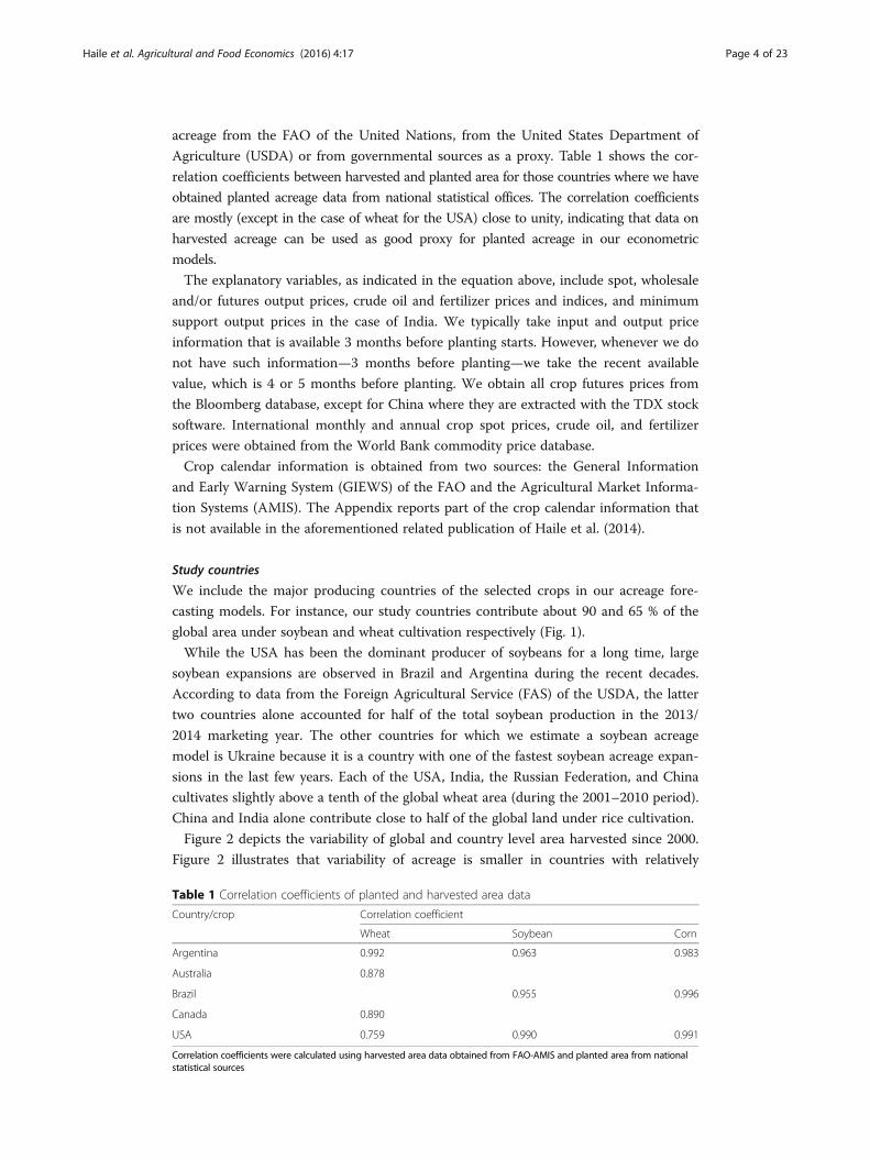
Agriculture (USDA) or from governmental sources as a proxy. Table 1 shows the cor-

relation coefficients between harvested and planted area for those countries where we have

obtained planted acreage data from national statistical offices. The correlation coefficients

are mostly (except in the case of wheat for the USA) close to unity, indicating that data on

harvested acreage can be used as good proxy for planted acreage in our econometric

models.

The explanatory variables, as indicated in the equation above, include spot, wholesale

and/or futures output prices, crude oil and fertilizer prices and indices, and minimum

support output prices in the case of India. We typically take input and output price

information that is available 3 months before planting starts. However, whenever we do

not have such information—3 months before planting—we take the recent available

value, which is 4 or 5 months before planting. We obtain all crop futures prices from

the Bloomberg database, except for China where they are extracted with the TDX stock

software. International monthly and annual crop spot prices, crude oil, and fertilizer

prices were obtained from the World Bank commodity price database.

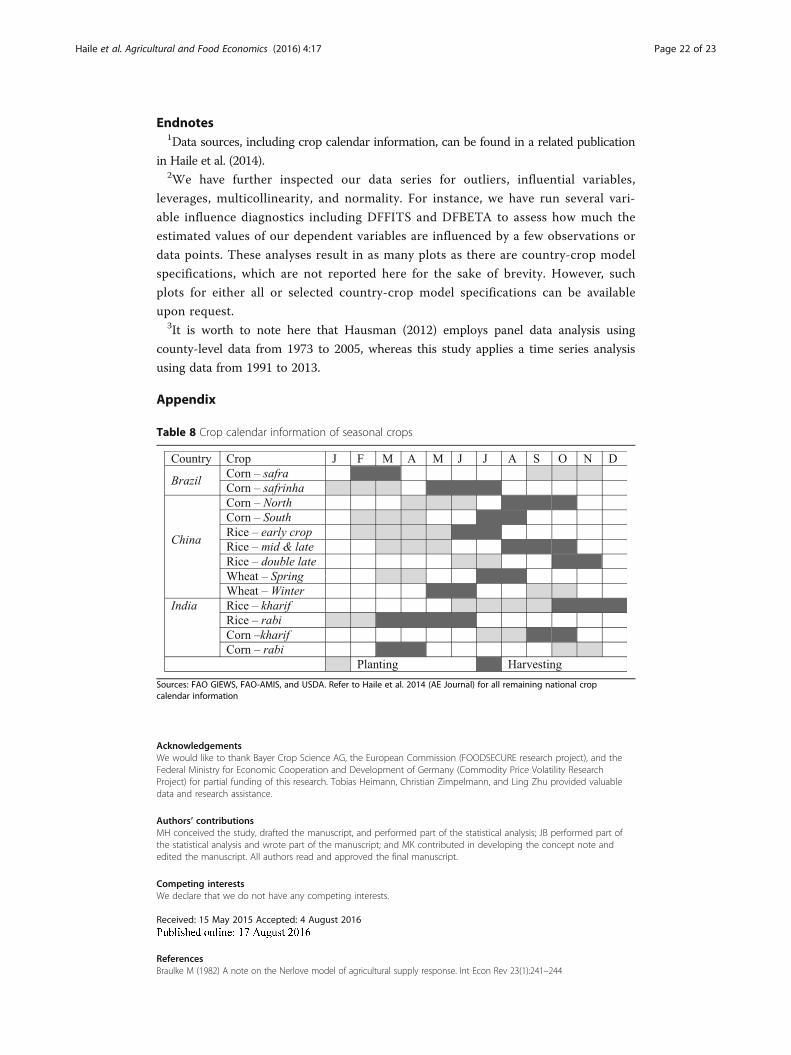
Crop calendar information is obtained from two sources: the General Information

and Early Warning System (GIEWS) of the FAO and the Agricultural Market Informa-

tion Systems (AMIS). The Appendix reports part of the crop calendar information that

is not available in the aforementioned related publication of Haile et al. (2014).

Study countries

We include the major producing countries of the selected crops in our acreage fore-

casting models. For instance, our study countries contribute about 90 and 65 % of the

global area under soybean and wheat cultivation respectively (Fig. 1).

While the USA has been the dominant producer of soybeans for a long time, large

soybean expansions are observed in Brazil and Argentina during the recent decades.

According to data from the Foreign Agricultural Service (FAS) of the USDA, the latter

two countries alone accounted for half of the total soybean production in the 2013/

2014 marketing year. The other countries for which we estimate a soybean acreage

model is Ukraine because it is a country with one of the fastest soybean acreage expan-

sions in the last few years. Each of the USA, India, the Russian Federation, and China

cultivates slightly above a tenth of the global wheat area (during the 2001–2010 period).

China and India alone contribute close to half of the global land under rice cultivation.

Figure 2 depicts the variability of global and country level area harvested since 2000.

Figure 2 illustrates that variability of acreage is smaller in countries with relatively

Table 1 Correlation coefficients of planted and harvested area data

Country/crop Correlation coefficient

Wheat Soybean Corn

Argentina 0.992 0.963 0.983

Australia 0.878

Brazil 0.955 0.996

Canada 0.890

USA 0.759 0.990 0.991

Correlation coefficients were calculated using harvested area data obtained from FAO-AMIS and planted area from nationalstatistical sources


larger area under cultivation of each crop. More specifically, we observe low area volatility

in big producers such as Brazil, China, India, USA, and the world aggregate, whereas we

observe large volatility of corn and wheat in Argentina, wheat in Canada, corn in Mexico,

and all crops in the Ukraine. The volatility of rice and wheat acreage is lower than the

volatility of soybean and corn acreage at a global level, whereas it depends on the size of

the area within each country. National policies, however, also play an important role for

affecting acreage volatility: Prices and input costs in countries with high government

subsidies like India are much more stable than in market-oriented economies like the

USA. However, larger price volatility may mean more volatile acreage allocation.

As shown in a related research paper by Haile et al. (2015), global short-term yield

response to prices and price risk is of similar magnitude to global acreage response. In other

words, higher crop prices are an incentive not only to expand crop acreage but also to in-

tensify production and to invest into higher yields through larger applications of modern in-

puts, crop protection, and other land management efforts. Forecasting acreage is therefore

an important first step in understanding and predicting the entire production of the major

crops. In this section, we provide brief background information on our study countries.

Fig. 1 Acreage share of countries included in our forecasting tool

Fig. 2 Volatility (standard deviation of the log returns) of different crops in different countries (data from2000 to 2014). Notes: We find the rule of thumb that the bigger the area of a specific crop in a specificcountry, the lower the volatility


Argentina is one of the major exporters of soybeans, typically after it is processed

within the country. As a result, soybean area has steadily increased over the past

25 years. Consequently, Argentina comprises of close to 20 % of the global land under

soybean cultivation as of the decade 2000–2010 (on average). There are two soybean

seasons in Argentina: harvest of the major soybean season starts in April before the

minor one starts a month later. For our analyses, we use domestic output prices in

pesos per ton instead of international prices since domestic prices exhibited higher

increases in level and variability following several exchange rate policy adjustments in

the country over the course of the study period. The domestic prices are obtained from

the Integrated Agricultural Information System (SIIA) of Argentina. However, inter-

national prices are considered for wheat acreage as the model fit improves.

Australia is one of the world’s key exporters of wheat although it only comprises

slightly above 5 % of the global wheat area cultivation. Some studies indicate that the

Australian wheat harvest failure contributed to the 2007–2008 price spikes (Trostle

2008; von Braun and Tadesse, 2012). The Australian global share of land acreage

allocated for soybeans and corn is relatively small, and that of rice is negligible. Conse-

quently, we estimate a model for Australian wheat acreage only. We obtain planted

wheat acreage data from the Australian Government Department of Agriculture and

Australian wheat prices from the Economic Research Service (ERS) of the USDA.

Brazil is a key producer of soybeans and corn accounting for about a quarter and a

tenth of the global soybean and corn cultivation, respectively. Harvesting of the first

out of the two corn seasons takes place in late February and March, while the second

harvest is between May and July (see Appendix). Production of the first corn is largely

used for the domestic feed market, whereas the second corn is primarily exported

(USDA 2013b). Traditionally, first-crop corn had been the larger of the two while the

second-crop corn was labelled as safrina (little crop). Yet, there seems to be a tendency

of moving to the second corn in Brazil in recent years arriving at 55 % second-season

corn production in 2012/2013. Since Brazilian farmers are typically large and commer-

cialized, we used futures prices from the Chicago Board of Trade (CBOT) to proxy

farmers’ price expectations. March corn and soybean futures prices are used for the

first corn and soybean acreage and September corn futures prices for the second corn

season. These futures are traded 3 months before planting starts.

Canada is a key producer of wheat, and it exports wheat mostly to the European

Union and to a small extent to the USA. Planting of wheat takes place in the spring

season. We obtain planted wheat acreage data from CANSIM—Canadian socioeco-

nomic database of statistics Canada. Fertilizer and crude oil prices are obtained from

the World Bank commodity price database, and we use futures prices traded at the

CBOT 3 months before planting starts in Canada.

China is the biggest producer of rice and wheat and an important producer of corn and

soybeans. Corn, soybeans, and wheat are mainly produced in the North, whereas rice is

mainly grown in the South with the Yangtze River as an approximate boundary. There are

three different seasons for rice: early crop rice is grown in southern provinces and along the

Yangtze River and consists mostly of indica rice; intermediate (mid) and single-crop late rice,

mostly japanoica, is grown in the southwest, the northern areas as well as along the Yangtze

River. Double-crop late rice is grown after harvest of the early crop in the southeastern parts

and constitutes a second indica crop where rice is grown. Therefore, indica prices have been


used for the estimations of the early and late rice whereas japanoica rice prices have been

used for the middle rice estimations. Depending on the region, there are different seasons for

corn and wheat. As more than 70 % of the corn is grown in the North, the estimation is done

using data available 3 month before planting in the North. Winter wheat constitutes about

90 % of the total wheat production in China. International prices as well as national future

prices are used for the forecast. As future prices are only available from 1995, 2000, and 2006

for soybeans, wheat, and corn, respectively, international prices, converted into Yuan with

the appropriate exchange, were used for the time period before. Data for the crop futures

was obtained with the free TDX stock software. Daily data is provided for the futures and the

exchange rate, so the monthly averages were calculated from this data. All prices were de-

flated by the consumer price index (CPI). A continuous CPI with 1990 as base year was con-

structed from the CPI data which is provided as a change for the last 12 month, i.e., for every

month, the index is 100 for the same month in the previous year.

India has the biggest wheat and rice areas in the world. However, due to low yields, it

is the second biggest producer after China. Furthermore, India is a big producer of

soybeans and corn. Areas for wheat, corn, and rice have slightly increased in recent

years while they have increased significantly for soybeans. There are two seasons for

rice and corn but only one for wheat and soybeans. For both rice and corn, kharif is

the main season with around 85 % of the total production volume for each crop while

the remainder is harvested in the less important rabi season. Yearly minimum support

prices (MSP) are set a couple of month before planting by the central government,

sometimes with top-ups by federal states. These open-end procurement prices are

guaranteed to farmers who sell to the government but higher profits may be obtained

by selling to private market actors if the market prices are higher. Apart from setting

these MSPs, there are many other government market interventions including large

public stock holding and grain subsidy. Data on area planted are neither reliable nor

continuously available leading to the use of the harvested area as a proxy. To account

for both the possibility to sell to the government for the guaranteed MSP and to sell to

private market actors for potentially higher wholesale price, the regressions use the

MSPs as well as the difference between the MSP and wholesale prices. All prices were

deflated by the CPI. Therefore, season-wise data was obtained from the Commission

for Agricultural Costs and Prices. For rice, no good prediction could be obtained with-

out including rainfall. Rainfall during planting time seems to play an important role for

cultivation of rice in India. Because rainfall data are not available in advance, the fore-

casting accuracy of our Indian rice acreage model is poor.

Kazakhstan is an important producer of cereals (mainly wheat) in Central Asia.

Wheat acreage in Kazakhstan accounts for about 6.5 % of the global acreage share in

2012. The bulk of the crop is sown in the spring season—in April and in May. The

total area planted under wheat represents over 85 % of total cereal production in the

country. Given the small share of other grains such as corn and soybeans in the country,

we have developed a model for forecasting wheat acreage only. We used international

monthly prices 3 months before planting of wheat in Kazakhstan in our wheat

acreage response model. Harvested wheat area from the USDA is used as a proxy

for planted acreage.

In Mexico, corn is by far the most important agricultural commodity in terms of both

production and consumption. Mexico is the sixth largest corn producing country in the


world, contributing above 5 % of the global land under corn cultivation. However, it is

also a key importer of corn. Corn is produced in all regions of the country and grows

throughout the year. While the spring-summer corn is sown between April and

September, the fall-winter corn is harvested October through March in the next calen-

dar year. The spring-summer season corn accounts for about three quarters of the total

corn production in the country. Because corn is used as both food and feed, Mexico—-

despite its high production—stands to be one of the world’s largest corn importers,

where the USA has been by far the largest supplier (USDA 2013a).

The Russian Federation is a key producer of wheat. It constitutes slightly above 10 %

of the global area under wheat cultivation. Wheat production in Russia has been more

or less constant over the past two decades, ranging between 20 and 25 million hectares.

However, there is a recent increase in production of corn and soybeans, especially since

2006/07. About two thirds of the total wheat production is usually winter wheat, which

is planted September through October.

Ukraine has become an important producer of corn and soybeans in recent periods,

although wheat covers a larger area. Planting of soybean and corn takes place during

the spring season, whereas about 95% of Ukraine wheat is winter wheat. Wheat is

planted in autumn. We use the monthly international prices from the World Bank

commodity price database to forecast these crop areas in Ukraine.

The USA is a major producer of corn, soybeans, and wheat. It is the world’s largest

producer and exporter of corn while constituting about a fifth of the global area culti-

vation. Soybeans rank second among the most-planted field crops in the USA making

it the largest producer and exporter of this oil crop. The USA cultivates about a third

of the global soybean acreage, produces about 10 % of the world’s wheat, and supplies

about a quarter of the world’s wheat exports. About a third of the total wheat produc-

tion in the US is planted in the winter season. As a result of their global importance,

we estimate acreage response models for all three crops. Planted acreage is obtained

from the USDA website and futures prices from the CBOT exchange serve as good

proxies for US farmers’ price expectations.

Estimation technique

Using a times-series approach, the acreage demand equations can be specified as a

linear function of the following form:

At;i ¼ β0;i þXn

jαij Et pij

� �þ β1Zt−1;i þ γt þ εt;i ð2Þ

where At,i denotes the acreage planted to the ith crop (i ∈ {wheat, corn, soybeans, rice}).The time trend captures smooth trends in such as technological changes or output

demand changes resulting from increased biofuel mandates, income, or population. All

the other variables are as defined above.

Our general procedure is to have different model specifications for each country

and each crop which differ based on the crop calendar and other characteristics of

the country, including planting and harvesting time, existence of futures exchange,

and relevance of competing crops. This gives us a set of a priori specifications

based on theoretical considerations. We then run regression models on the re-

spective model specifications with different crop prices (e.g. domestic wholesale


spot prices, futures prices, international spot prices) and input prices (fertilizer and

oil prices). After testing several model specifications, we ultimately choose the

model with the highest predictive power adjusted for the number of explanatory

variables (adjusted R2) and with the smallest root mean squared error (RMSE). The

final model is the one that best explains acreage with the minimum input data re-

quirement. Models that use data not easily available a few months before planting

(e.g., rainfall) were considered only if the predictive power remained too low other-

wise. We have taken special care in comparing estimates from alternative model

specifications by retaining the same dependent variable. In order to minimize the

risk of a pre-test bias, we additionally considered the Bayesian information criter-

ion (BIC) for our model selection.

While higher own crop prices imply larger expected profits for acreage expansion

(positive coefficient), higher prices of competing crops induce producers to shift

land away from the respective crop (negative coefficient). Fertilizer and oil prices

indicate production costs, and the higher such costs, the lower the incentive to

cultivate more land. Thus, we expect a negative coefficient for these variables.

However, higher oil price also indicate more demand for biofuel and may have a

positive coefficient, especially for corn. High fertilizer prices may also have a posi-

tive effect on the acreage of some crops. This is typically the case for soybeans.

Soybean production requires little or no nitrogenous fertilizer and higher fertilizer

prices therefore may imply that it is less costly to allocate more land for soybean

production, shifting away from crops with large fertilizer demand. With the coeffi-

cients of these variables for each country and each crop, it would then be possible

to forecast acreage.

All variables in the acreage response model in Eq. (2) are transformed to their logarithmic

formats in the respective econometric models. Hence, the estimated coefficients can be

interpreted as acreage elasticities. Therefore, to calculate the total area, one cannot just take

the exponential of the estimated logged variable. Instead, given equation (2) above, one has

to calculate A ¼ α0 exp dlog A� �

where the “hat” implies that the variables are estimated

and α0 ¼ 1n

Xi¼1

n exp εið Þ where n is the total number of observations (Wooldridge 2009).

Before conducting our estimation, however, we need to check for the stationarity of

our time series variables. We use the Augmented Dickey-Fuller (ADF) unit root test for

this purpose. The results from the ADF test, available upon request, show that nearly

all our time series variables exhibit non-stationarity at the 5 % level of statistical signifi-

cance. Few exceptions with stationary variables include corn and soybean prices in the

Indian Kharif corn acreage model; corn acreage in Mexico; wheat acreage in Ukraine;

and soybean acreage in Argentina.

Similarly, we test for unit root of all of the time series variables after first differ-

encing. The unit root test results indicate that nearly all the variables in the acre-

age response models are stationary after first differencing at the 10 % level or less

(Table 2). Thus, we instead use the first order difference variables, which are I(0) series,

for the empirical model estimations to avoid spurious regression results. The constant is

therefore interpreted as a linear trend in the empirical estimations. Furthermore, because

autocorrelation is typically a problem in time series models, the Newey-West autocorrel-

ation adjusted standard errors are employed in the econometric estimations.2


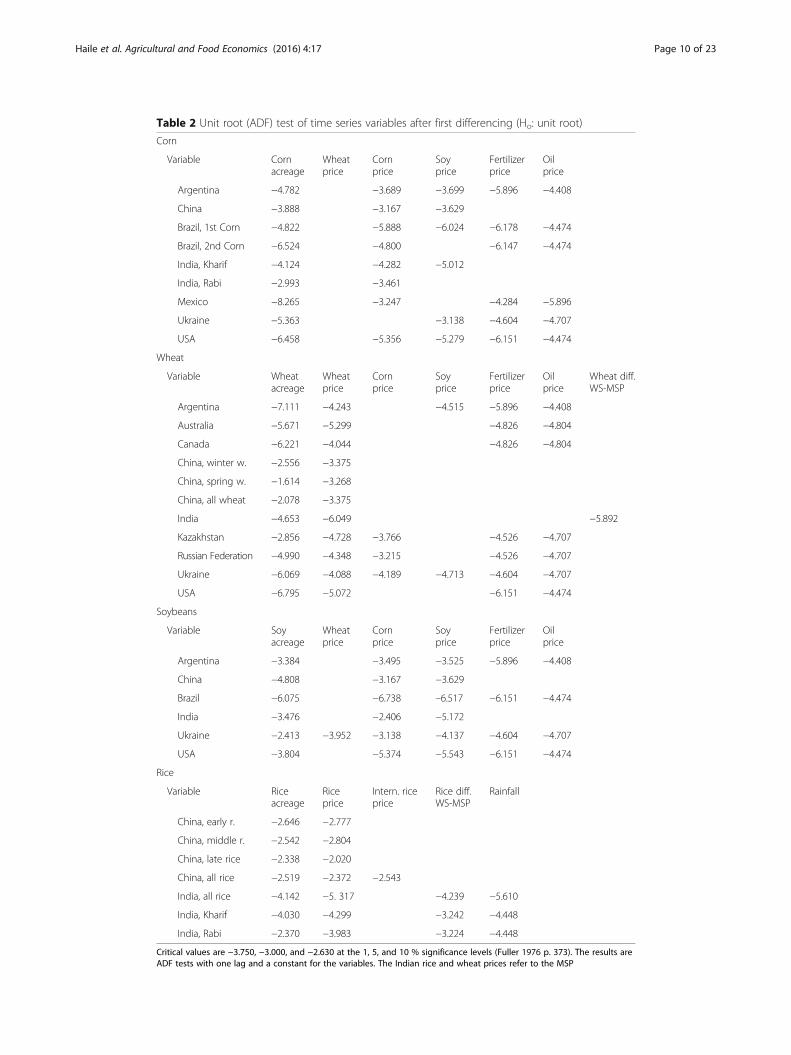
Table 2 Unit root (ADF) test of time series variables after first differencing (Ho: unit root)

Corn

Variable Cornacreage

Wheatprice

Cornprice

Soyprice

Fertilizerprice

Oilprice

Argentina −4.782 −3.689 −3.699 −5.896 −4.408

China −3.888 −3.167 −3.629

Brazil, 1st Corn −4.822 −5.888 −6.024 −6.178 −4.474

Brazil, 2nd Corn −6.524 −4.800 −6.147 −4.474

India, Kharif −4.124 −4.282 −5.012

India, Rabi −2.993 −3.461

Mexico −8.265 −3.247 −4.284 −5.896

Ukraine −5.363 −3.138 −4.604 −4.707

USA −6.458 −5.356 −5.279 −6.151 −4.474

Wheat

Variable Wheatacreage

Wheatprice

Cornprice

Soyprice

Fertilizerprice

Oilprice

Wheat diff.WS-MSP

Argentina −7.111 −4.243 −4.515 −5.896 −4.408

Australia −5.671 −5.299 −4.826 −4.804

Canada −6.221 −4.044 −4.826 −4.804

China, winter w. −2.556 −3.375

China, spring w. −1.614 −3.268

China, all wheat −2.078 −3.375

India −4.653 −6.049 −5.892

Kazakhstan −2.856 −4.728 −3.766 −4.526 −4.707

Russian Federation −4.990 −4.348 −3.215 −4.526 −4.707

Ukraine −6.069 −4.088 −4.189 −4.713 −4.604 −4.707

USA −6.795 −5.072 −6.151 −4.474

Soybeans

Variable Soyacreage

Wheatprice

Cornprice

Soyprice

Fertilizerprice

Oilprice

Argentina −3.384 −3.495 −3.525 −5.896 −4.408

China −4.808 −3.167 −3.629

Brazil −6.075 −6.738 –6.517 −6.151 −4.474

India −3.476 −2.406 −5.172

Ukraine −2.413 −3.952 −3.138 −4.137 −4.604 −4.707

USA −3.804 −5.374 −5.543 −6.151 −4.474

Rice

Variable Riceacreage

Riceprice

Intern. riceprice

Rice diff.WS-MSP

Rainfall

China, early r. −2.646 −2.777

China, middle r. −2.542 −2.804

China, late rice −2.338 −2.020

China, all rice −2.519 −2.372 −2.543

India, all rice −4.142 −5. 317 −4.239 −5.610

India, Kharif −4.030 −4.299 −3.242 −4.448

India, Rabi −2.370 −3.983 −3.224 −4.448

Critical values are −3.750, −3.000, and −2.630 at the 1, 5, and 10 % significance levels (Fuller 1976 p. 373). The results areADF tests with one lag and a constant for the variables. The Indian rice and wheat prices refer to the MSP


Limitations with regard to our acreage forecast

It is important to be aware of some limitations of our modeling approach, especially

with regard to using the estimates for forecasting purposes. One challenge of supply

estimates is the limited amount of observations for aggregated national data. Since the

empirical models are based on prices as the most important (and easily measureable)

determinants of supply response, they will have limited predictive power in cases where

non-price factors are more important. This may be the case if i) governments imple-

ment ad hoc policies and controls; (ii) farmers produce crops mainly for their own con-

sumption; (iii) farmers have limited market access; (iv) farmers selling prices are

systematically different from the reference prices we consider (e.g., in case of imperfect

price transmission or non-convergence of futures and spot prices); or (v) other subsid-

ies and taxes dilute the incentive role of prices.

As explained above, spot prices at planting time are often good proxies for expected

futures prices because there is an inter-temporal dynamic relationship between the two

price series. This relationship, however, can change if interest rates, storage costs or

storage policies change or if stocks are depleted. Finally, our model assumes a stable re-

lationship between acreage and the explanatory variables, which might be inappropriate

for countries experiencing large transformations. To reduce this problem, we typically

considered periods after 1991.

Results and discussionRegression results

Tables 3, 4, 5, and 6 present the regression results for the acreage response models of

corn, wheat, soybeans, and rice, respectively. In general, the regression estimates illustrate

that own and competing crop prices have positive and negative coefficients respectively,

consistent with economic theory. The joint F-test results, which are reported at the bot-

tom of each table, indicate that the acreage models (except in a few cases) are statistically

reliable. The adjusted R2 values are sometimes small but this is not unexpected in time

series models with first differences. In some models, the lagged area is included while it is

excluded in others. In general, the lagged area should only be included if it increases the

explanatory power of the model. Three criteria are used to decide on this: adjusted R2,

BIC, and the statistical significance of the autoregressive coefficient. Usually, these criteria

all suggest the use of the same model; whenever they do not, the model that is supported

by two of these criteria is chosen. In the last row of the tables, it is indicated which criteria

have justified the specific choice.

Corn acreage responds to its own prices with elasticities that range from negligible in

Ukraine to as high as 0.6 for second corn in Brazil (Table 3). A 10 % higher corn price,

for instance, leads to an expansion of corn acreage by about 4 % in Argentina and by

about 6 % of the second corn in Brazil. Not only is the price response of the second-

crop corn (also called safrinha) in Brazil stronger, it also has a strong positive time

trend as reflected by the statistically significant intercept term. In agreement with this

finding, the data show that area under cultivation of safrinha corn in Brazil took the

lead over the first corn (also called safra) during the 2012 planting season. Not surprisingly,

the intercept term of the first corn crop is statistically significant and negative, indicating its

declining trend. US corn acreage responds to own crop price relatively strongly. All other


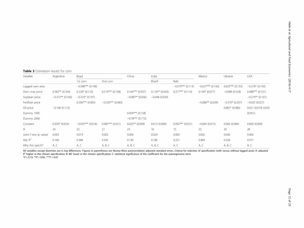
Table 3 Estimation results for corn

Variable Argentina Brazil China India Mexico Ukraine USA

1st corn 2nd corn Kharif Rabi

Lagged own area −0.588*** (0.196) −0.579*** (0.113) −0.637*** (0.150) 0.655*** (0.153) −0.276* (0.150)

Own crop price 0.382** (0.164) 0.228* (0.123) 0.574*** (0.138) 0.164*** (0.037) 0.124** (0.043) 0.377*** (0.114) 0.140* (0.077) −0.088 (0.328) 0.488*** (0.101)

Soybean price −0.372** (0.166) −0.333* (0.197) −0.085** (0.036) −0.048 (0.034) −0.274** (0.101)

Fertilizer price 0.206*** (0.065) −0.250*** (0.083) −0.086** (0.039) −0.370* (0.207) −0.035 (0.027)

Oil price −0.108 (0.113) 0.882* (0.486) 0.021 (0.019) 0.035

Dummy 1995 0.454*** (0.158) (0.051)

Dummy 2006 −0.78*** (0.173)

Constant 0.050* (0.024) −0.055*** (0.016) 0.085*** (0.021) 0.023** (0.009) 0.013 (0.008) 0.092*** (0.021) −0.004 (0.015) 0.066 (0.084) 0.000 (0.009)

N 24 22 21 23 16 15 22 20 28

Joint F-test (p value) 0.003 0.019 0.002 0.000 0.029 0.000 0.002 0.040 0.000

Adj. R2 0.166 0.388 0.342 0.130 0.186 0.221 0.484 0.326 0.557

Why this specif.? A, C A, C A, B, C A, B, C A, B, C A, C A, C A, B, C A, C

All variables except dummies are in log differences. Figures in parentheses are Newey-West autocorrelation adjusted standard errors. Criteria for selection of specification (with versus without lagged area): A: adjustedR2 higher in the chosen specification; B: BIC lower in the chosen specification; C: statistical significance of the coefficient for the autoregressive term*P < 0.10, **P < 0.05, ***P < 0.01

Haile

etal.A

griculturalandFood

Economics

(2016) 4:17 Page

12of

23

Table 4 Estimation results for wheat

Variable Argentina Australia Canada China India Kazakhstan Russia Ukraine USA

Winter Spring Total

Lagged ownarea

−0.220 (0.144) 0.380** (0.160) 0.379*** (0.132) −0.563***(0.152)

−0.438** (0.179)

Own cropprice

0.141 (0.172) 0.140 (0.093) 0.103** (0.050) 0.039 (0.024) 0.160 (0.107) 0.052** (0.024) 0.123* (0.067)(MSP)

−0.011 (0.064) 0.172** (0.070) 0.355* (0.208) 0.286** (0.121)

Soybeanprice

0.023 (0.253) 0.052 −0.093 (0.528) −0.069 (0.089)

Corn price (0.061) −0.210** (0.090) −0.348 (0.361) −0.052 (0.102)

Fertilizerprice

−0.345*** (0.117) 0.210** (0.073) 0.159** (0.045) −0.003 (0.065) 0.123 (0.191) 0.021 (0.019)

Oil price −0.263*** (0.085) 0.173** (0.067) 0.262*** (0.071)

Diff. MSP-WSP

0.022* (0.012)

Dummy2000

−0.128 (0.114) −0.880 (0.517) −0.285** (0.109)

Constant −0.007 (0.027) 0.022 (0.018) −0.026 (0.014) −0.005 (0.011) −0.039 (0.026) −0.002 (0.006) 0.005 (0.006) −0.017 (0.018) −0.023 (0.018) 0.002 (0.050) −0.017** (0.007)

N 23 23 23 20 20 22 29 20 20 20 28

Joint F-test(p value)

0.056 0.032 0.007 0.001 0.001 0.000 0.123 0.311 0.008 0.594 0.018

Adj. R² 0.214 0.301 0.335 0.034 0.020 0.262 0.050 0.061 0.465 −0.068 0.286

Why thisspecif.?

B, C A, B A, B, C A, (B), C A, B, C A, B, C A, C A, C A, C A, B, C A, B, C

All variables except dummies are in log differences. Figures in parentheses are Newey-West autocorrelation adjusted standard errors. Criteria for selection of specification (with versus without lagged area): A: adjustedR2 higher in the chosen specification; B: BIC lower in the chosen specification; C: statistical significance of the coefficient for the autoregressive term*P < 0.10, ** P <0.05, *** P <0.01

Haile

etal.A

griculturalandFood

Economics

(2016) 4:17 Page

13of

23

Table 5 Estimation results for soybeans

Variable Argentina Brazil China India Ukraine USA

Lagged own area 0.196* (0.097) 0.493** (0.206)

Own crop price 0.061 (0.059) 0.340* (0.181) 0.300** (0.124) 0.157* (0.084) 0.609 (0.546) 0.265** (0.120)

Corn price −0.067 (0.059) −0.203* (0.124) −0.476*** (0.150) −0.046 (0.170) −0.178 (0.457) −0.255* (0.145)

Wheat price −0.993* (0.582)

Fertilizer price −0.042 (0.038) −0.086* (0.046) −0.231* (0.136) 0.025 (0.023)

Dummy 1995 −1.504** (0.552)

Dummy 2006 2.244*** (0.704)

Constant 0.060*** (0.014) 0.040*** (0.013) −0.007 (0.013) 0.039* (0.019) 0.146* (0.082) 0.005 (0.009)

N 24 23 23 17 19 28

Joint F-test (p value) 0.24 0.058 0.000 0.147 0.056 0.016

Adj. R2 0.121 0.199 0.415 0.068 0.347 0.294

Why this specif.? A, C A, B, C A, B, C A, B, C A, B, C A, C


Haile

etal.A

griculturalandFood

Economics

(2016) 4:17 Page

14of

23

Table 6 Estimation results for Rice

Variable China India

Early Middle Late Total Kharif Rabi Total

Lagged own area −0.532*** (0.081) 0.593*** (0.127)

Own domestic crop price 0.302*** (0.068) 0.134* (0.074) 0.302*** (0.030) 0.230*** (0.061) 0.189 (0.126) 0.251 (0.429) 0.156 (0.092)

Rainfall 0.201*** (0.049) 0.481* (0.225) 0.161*** (0.056)

Difference MSP-WSP 0.033*** (0.009) 0.063* (0.033) 0.012* (0.006)

Dummy 2008 −0.073** (0.024)

Constant −0.033*** (0.009) 0.017 (0.007) −0.016** (0.007) −0.011** (0.005) −0.003 (0.005) 0.004 (0.035) 0.000 (0.005)

N 13 13 14 15 16 16 23

Joint F-test (p value) 0.001 0.000 0.000 0.001 0.001 0.042 0.038

Adj. R2 0.459 0.474 0.768 0.562 0.563 0.230 0.365

Why this specif.? A, B, C A, B, C A, B, C A, B, C A, B, C A, B, C A, B, C


Haile

etal.A

griculturalandFood

Economics

(2016) 4:17 Page

15of

23

factors remaining constant, a 10 % increase in corn price induces about a 5 % expansion of

corn acreage in the USA. Acreages of both kharif and rabi corn in India fairly respond to

own crop prices, with short-term elasticities of 0.12 and 0.38, respectively. Not only is the

acreage of Rabi corn in India three times more responsive to own crop prices than kharif

corn, it also has a significant positive time trend. According to the result, acreage of the In-

dian rabi corn has been growing by an annual rate of about 9 %. A rise in own crop price

also leads to a statistically significant corn acreage response in China, with a short-term

elasticity of 0.16. Corn competes for land (and other inputs) primarily with soybeans. This

is reflected by the statistically significant and negative corn-soybean cross price elasticity of

corn acreage in most countries including in Argentina, Brazil, China, and the USA.

While corn acreage negatively responds to fertilizer price index (except safra in

Brazil), it has statistically insignificant response to international crude oil prices (with

an exception of Ukraine). As it is theoretically expected, high (input) fertilizer price

reduces producers’ profit expectations and they tend to shift land away to crops with

little or no fertilizer demand. In contrast, a high crude oil price has two opposite

effects. On the one hand, higher oil price implies large production cost and hence its

effect is expected to be negative. On the other hand, higher oil price imply larger

demand for biofuel, and hence for corn, and hence its acreage effect is positive. The

net effect seems to be statistically negligible in our empirical estimations, except in

Ukraine where the positive demand effect outweighs.

Although elasticities are smaller than for the corn acreage model, wheat acreage in

our study countries exhibits a positive response to own prices (Table 4). Price elastici-

ties of wheat acreage range from about negligible in a few countries to about 0.4 % in

Ukraine. More specifically, a 10 % higher wheat price induces an expansion of wheat

acreage by about 4 % in Ukraine, 0.3 % in the USA, 0.2 % in the Russian Federation,

and by about 1 % in each of India, Canada, and China (total wheat). In addition to the

MSP, Indian wheat acreage has a statistically significant positive response to the differ-

ence between the MSP and the wholesale price. It is also interesting to see that wheat

acreage in most of the countries does not show any significant trend over time except

in the USA, where it has an annual declining trend of about 2 %. Furthermore, it is also

noteworthy to mention the positive coefficient of the international oil price on the

wheat acreages of Kazakhstan and the Russian Federation, which is contrary to our ex-

pectations. One explanation could be that larger export revenues as a result of higher

international oil prices might have a substantial share in the national incomes of these

countries and these might (partly) be invested into agriculture.

The results for soybeans are reported in Table 5. Overall soybean acreage positively

responds to own prices and negatively to competing crop prices as expected. High

fertilizer prices reduce soybean area in Brazil and Ukraine. High levels of price respon-

siveness are found in Brazil, Ukraine, the USA, and China, whereas lower levels are

found in India and Argentina. Our estimated soybean price elasticity of acreage for

Brazil (0.34) lies between the spot (0.26) and futures (0.63) price acreage elasticities

estimated by Hausman (2012).3 For China, two dummies have been included because

the time series for the prices changed from international price to domestic future

prices. Except for China, the constant is positive indicating that soybean area has an in-

creasing trend in the long run. This positive trend is especially high for Ukraine, illus-

trating the recent rapid soybean acreage expansion in the country. Such trend may be


the result of increases in population, income, consumer preferences, and technology.

These factors seem to put pressure on land availability for soybean production in most

countries.

Table 6 reports the results for rice acreage response. We model rice acreage response

in China and India, where half of the world’s rice cultivation takes place. Seasonal rice

as well as total acreage responses are investigated in both countries. A small number of

observations have often prevented us to include more than one or two explanatory

variables. Wholesale prices in China are not consistently available for earlier years and

international prices turned out to have no predictive power, which is why they are not

reported here. This is not surprising because smallholder farmers in both countries do

not usually have access to international markets and trade restrictions often limit inter-

national price transmission to domestic market. For the individual season rice in China,

forecasts are not possible because last year’s area and prices reported in the yearbooks

are only available ex post, i.e., a few months after the harvest.

However, for the total area, timely available acreage data were taken from the FAO

and prices from the agricultural ministry website. This enables forecasting the total rice

acreage. A dummy for the year 2008 is included because earlier domestic prices are

available from the yearbooks, whereas the later ones are obtained from the TDX soft-

ware. Competing crop, oil, and input prices are tested but are found to be statistically

insignificant and therefore are not reported. The lagged area changes are included for

the middle and late rice area in China.

While no clear time trend of the rice area is visible in India, in China there is mostly

a slow decrease indicated by the negative constant term. The own price responsiveness

is relatively high in both countries but it is statistically significant only in China. In

India, the MSP was used as “own domestic crop price” and it has a higher effect than

the difference between the wholesale price and the MSP, but the latter is more signifi-

cant and therefore more consistent among the indsividual observations. As expected,

all price variables have positive signs. However, including rainfall makes results much

better India. The results show that rainfall is the most important driver of Indian rice

area. This limits the area forecasting possibility of the empirical model since predicting

rainfall is difficult if not impossible. Interestingly, including a rainfall variable is suffi-

cient to obtain a good fit.

Validation of forecasting power

In order to examine the forecasting power of our models, we use two types of tests.

One is a simple quality check of the fitted values to illustrate the level of the residuals.

These are the residuals for years that are part of the sample and that we used in the

regression. Figure 3 depicts our estimation results—including also the 50 and 90 %

confidence intervals—and compares them with the actually observed values for a selec-

tion of crops and countries.

Confidence intervals are based on OLS standard errors. We only show a selection of

the fitted graphs here; all figures are available upon request. In general, the estimations

performed well in predicting the actual values. However, there are some outliers and

these mostly occur when there are big sudden changes. Nevertheless, the predictions

have often the same direction of change as that of the observed data. Looking at


soybean area in China, for example, shows that in the year 1993 a big increase in area

was forecasted but the actual increase was a lot higher and therefore is even out of the

confidence interval. The same holds for the large decline in wheat area in China in the

year 2000 where a much smaller decline was predicted. Sometimes but rarely, there are

outliers which are not in the confidence intervals an even the direction of change was

not predicted correctly as it is the case for the soy are in China in the year 2000. For

some countries and crops, the confidence intervals are relatively large while they are

Fig. 3 Comparison of ex-post estimations and confidence intervals with observed area data. Notes: For eachcrop, two countries are shown as an example except for rice, where only India is shown


smaller for others like wheat in China, corn in the US, or rice in China (consider the

scale). Interestingly, the large increase in corn area in the USA in 2007 due to the

biofuel mandates are well captured in the graph for corn, whereas the accompanying

decrease in soy area in that year is not captured in the graph.

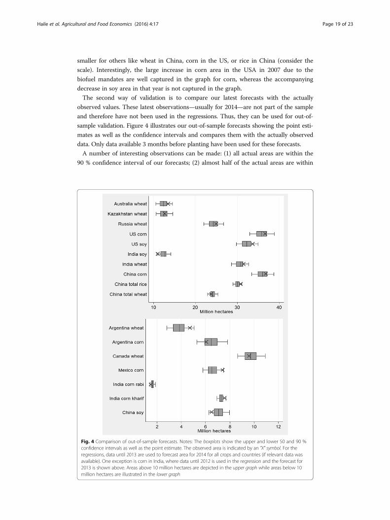
The second way of validation is to compare our latest forecasts with the actually

observed values. These latest observations—usually for 2014—are not part of the sample

and therefore have not been used in the regressions. Thus, they can be used for out-of-

sample validation. Figure 4 illustrates our out-of-sample forecasts showing the point esti-

mates as well as the confidence intervals and compares them with the actually observed

data. Only data available 3 months before planting have been used for these forecasts.

A number of interesting observations can be made: (1) all actual areas are within the

90 % confidence interval of our forecasts; (2) almost half of the actual areas are within

Fig. 4 Comparison of out-of-sample forecasts. Notes: The boxplots show the upper and lower 50 and 90 %confidence intervals as well as the point estimate. The observed area is indicated by an "X" symbol. For theregressions, data until 2013 are used to forecast area for 2014 for all crops and countries (if relevant data wasavailable). One exception is corn in India, where data until 2012 is used in the regression and the forecast for2013 is shown above. Areas above 10 million hectares are depicted in the upper graph while areas below 10million hectares are illustrated in the lower graph


the 50 % confidence interval, which underlines the validity of our models; (3) while 11

times the actual values were higher than the forecast, they only were lower in 6 cases;

(4) the confidence intervals vary in size between the different crops and different countries.

Not only do the confidence intervals typically increase when the estimated area increases

but also significantly differ for comparable areas, thereby indicating that some forecasts

perform significantly better than others. And, (5) forecasts for individual seasons are mostly

impossible because the required data are not available in time. The upward-biased forecast

related to (3) is primarily driven by countries where we used international rather than do-

mestic prices. This could indicate a shift in the international price transmission dynamics

and can be indicative of the need to use domestic price data in order to improve acreage

forecasts.

Overall, the forecasts perform well even if many of them only provide a rough esti-

mation due to the wide confidence intervals. The predicted acreage is usually correct in

terms of direction. Moreover, the actual data points are mostly in the 90 % confidence

interval, showing a high prediction power when validated with historical data. However,

the forecasting precision varies significantly from crop to crop and country to country.

ConclusionsA substantial part of the analyses in this paper has been devoted to identify the relevant

determinants of acreage supply for each crop and country. This enables us to select the

model that provides the best prediction power (high explanatory power) with minimal

input data requirement. The price elasticity of acreage estimates are key parameters for

forecasting acreage in all the countries. Moreover, the acreage elasticity estimates can

serve as a ground proofing and robustness check for other studies that estimate world-

wide aggregate acreage elasticities (e.g., Haile et al. 2014). Worldwide aggregate acreage

elasticity estimates give an average effect of prices on acreage for each crop, whereas

country-specific acreage elasticities can be used as inputs in acreage forecasting appli-

cations for the respective countries and crops.

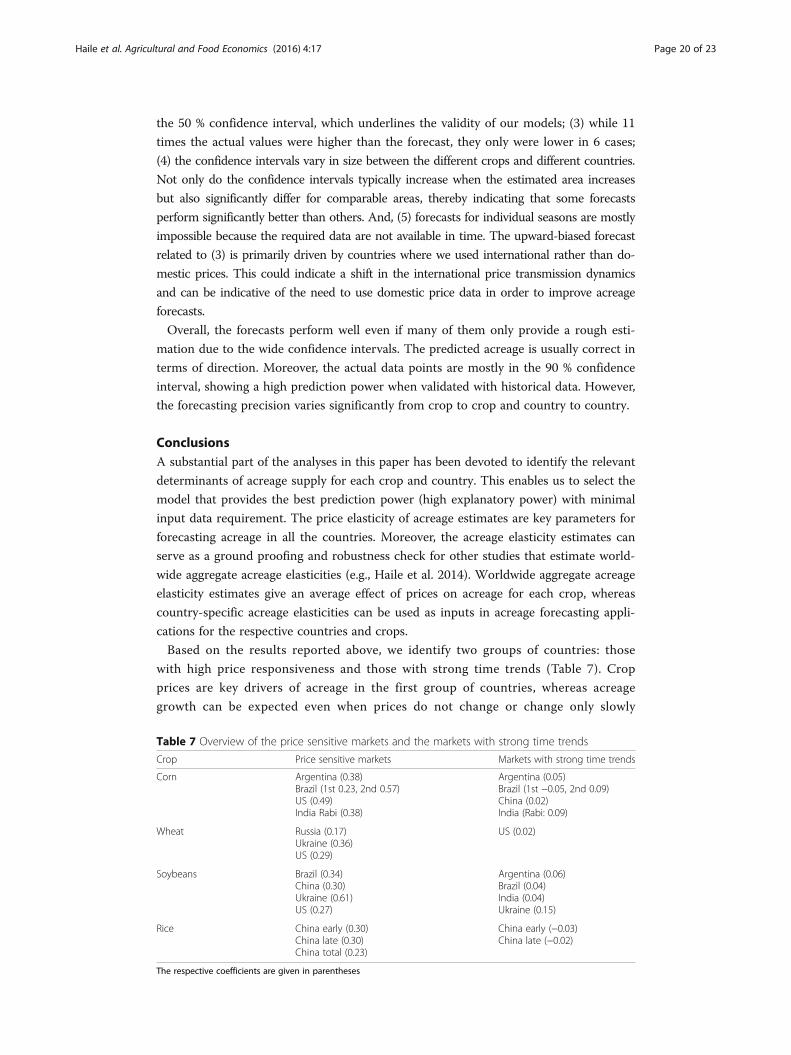
Based on the results reported above, we identify two groups of countries: those

with high price responsiveness and those with strong time trends (Table 7). Crop

prices are key drivers of acreage in the first group of countries, whereas acreage

growth can be expected even when prices do not change or change only slowly

Table 7 Overview of the price sensitive markets and the markets with strong time trends

Crop Price sensitive markets Markets with strong time trends

Corn Argentina (0.38)Brazil (1st 0.23, 2nd 0.57)US (0.49)India Rabi (0.38)

Argentina (0.05)Brazil (1st −0.05, 2nd 0.09)China (0.02)India (Rabi: 0.09)

Wheat Russia (0.17)Ukraine (0.36)US (0.29)

US (0.02)

Soybeans Brazil (0.34)China (0.30)Ukraine (0.61)US (0.27)

Argentina (0.06)Brazil (0.04)India (0.04)Ukraine (0.15)

Rice China early (0.30)China late (0.30)China total (0.23)

China early (−0.03)China late (−0.02)

The respective coefficients are given in parentheses


in the latter group of markets. These countries—countries that belong to both

groups—have large potential to boost food production and are therefore key in

tackling food insecurity and hunger, which are two of the greatest challenges of

our time. Countries in the first group respond to food scarcity more strongly,

which may suggest existence of sound market institutions. Regardless of market

conditions, countries in the second group have large potential (such as abundant

land) to produce more. All these countries have a vital role in supplying food to

the international market.

Crops with high price responsiveness (i.e., own price elasticity higher than or

equal to 0.2) include corn in Argentina, Brazil (both first and second corn), and

the USA and rabi corn in India; wheat in the Russian Federation, Ukraine, and the

USA; and soybeans in Brazil, China, Ukraine and the USA. Furthermore, acreages

of early, late, and total rice in China exhibit strong price responsiveness. These

findings are interesting from a policy perspective as they indicate institutional

differences across countries. While producers in countries with well-functioning

financial markets and input and output markets may benefit from higher output

prices, this may not be the case in countries where these markets do not exist or

function poorly. There are quite a few countries and crops where cropland is ex-

pected to grow or decline by more than 2 % per year regardless of changes in

prices or costs. Among these countries, soybeans in Ukraine, second corn in Brazil,

and rabi corn in India show the highest long-run acreage trends. In these coun-

tries, acreage expansion or shrinkage can be expected even if prices remain stable

or are slightly changing.

Input costs (fertilizer prices) are important factors for acreage response in most

cases. Less obvious is the crop acreage response towards higher oil prices, with

mixed (positive and negative) acreage response effects. For instance, increasing oil

prices boost acreage expansion in Kazakhstan and the Russian Federation—where

revenues from oil exports have a substantial share in respective national incomes

and it might be (partly) invested into agriculture.

While we are able to explain historical acreage fluctuations well for most countries

and crops, forecasting power is weak for some particular cases. Our model, for in-

stance, has weak explanatory power for wheat acreage in Ukraine and rice acreage in

India. Nevertheless, the ARDL acreage models adequately explain historical acreage

decisions. The results provide elasticities that can serve as a basis for a timely fore-

cast of upcoming planting season acreage based on the currently and publicly avail-

able data in most cases. The calculated point forecast is extended by an interval

estimation which helps to assess the likely range of the acreage allocation. This is im-

portant to appropriately deal with uncertainties and risks as forecasts are usually

uncertain.

It is worth to note that the forecasts are primarily based on price movements as

major determinants of acreage. The forecasting tool could therefore be extended by

further market analyses based on broader political and economic factors as well as

short-term weather events, which are not accounted for by prices but that could poten-

tially influence acreage decisions. Due to small size of observations, this is, however,

only possible with intra-country panel data or by pooling countries—the latter yielding

average acreage responses only.


Endnotes1Data sources, including crop calendar information, can be found in a related publication

in Haile et al. (2014).2We have further inspected our data series for outliers, influential variables,

leverages, multicollinearity, and normality. For instance, we have run several vari-

able influence diagnostics including DFFITS and DFBETA to assess how much the

estimated values of our dependent variables are influenced by a few observations or

data points. These analyses result in as many plots as there are country-crop model

specifications, which are not reported here for the sake of brevity. However, such

plots for either all or selected country-crop model specifications can be available

upon request.3It is worth to note here that Hausman (2012) employs panel data analysis using

county-level data from 1973 to 2005, whereas this study applies a time series analysis

using data from 1991 to 2013.

Appendix

AcknowledgementsWe would like to thank Bayer Crop Science AG, the European Commission (FOODSECURE research project), and theFederal Ministry for Economic Cooperation and Development of Germany (Commodity Price Volatility ResearchProject) for partial funding of this research. Tobias Heimann, Christian Zimpelmann, and Ling Zhu provided valuabledata and research assistance.

Authors’ contributionsMH conceived the study, drafted the manuscript, and performed part of the statistical analysis; JB performed part ofthe statistical analysis and wrote part of the manuscript; and MK contributed in developing the concept note andedited the manuscript. All authors read and approved the final manuscript.

Competing interestsWe declare that we do not have any competing interests.

Received: 15 May 2015 Accepted: 4 August 2016

ReferencesBraulke M (1982) A note on the Nerlove model of agricultural supply response. Int Econ Rev 23(1):241–244

Table 8 Crop calendar information of seasonal crops

Sources: FAO GIEWS, FAO-AMIS, and USDA. Refer to Haile et al. 2014 (AE Journal) for all remaining national cropcalendar information


Chavas JP, Holt MT (1990) Acreage decisions under risk: the case of corn and soybeans. Am J Agric Econ 72(3):529–538Coyle BT (1993) On modeling systems of crop acreage demands. J Agric Resour Econ 18(1):57–69Economic Research Service (ERS) - USDA (2013a) Corn:trade. Available at http://www.ers.usda.gov/topics/crops/corn/

trade.aspx. Accessed 14 July 2016.Fama EF, French KR (1987) Commodity futures prices: some evidence on forecast power, premiums, and the theory of

storage. J Bus 60(1):55–73FAO. (1996). Rome Declaration on World Food Security and World Food Summit Plan of Action (pp. 13–17). World

Food Summit: Rome, Italy.FAO. (2012). Agricultural Statistics, FAOSTAT. FAO (Food and Agricultural Organization of the United Nations). Rome,

Italy.FAO, IFAD, & WFP. (2015). The State of Food Insecurity in the World 2015. Meeting the 2015 international hunger

targets: taking stock of uneven progress. Rome, Italy: Food and Agriculture Organization of the United Nations.Foreign Agricultural Service (FAS) - USDA (2013b). Commodity intelligent report. Available at http://www.pecad.fas.

usda.gov/highlights/2013/05/br_15may2013/. Accessed 14 July 2016.Fuller W (1976) Introduce to statistical time series. Wiley, New YorkGardner BL (1976) Futures prices in supply analysis. Am J Agric Econ 58(1):81–84Haile MG, Kalkuhl M, von Braun J (2014) Inter- and intra-seasonal crop acreage response to international food prices

and implications of volatility. Agric Econ 45(6):693–710Haile MG, Kalkuhl M, von Braun J (2015) Worldwide acreage and yield response to international price change and

volatility: a dynamic panel data analysis for wheat, rice, corn, and soybeans. Am J Agric Econ 97(3):1–19Hausman C (2012) Biofuels and land use change: sugarcane and soybean acreage response in Brazil. Environ Resour

Econ 51(2):163–87Hernandez, M, & Torero, M (2010) Examining the dynamic relationship between spot and future prices of agricultural

commodities: IFPRI Discussion Paper 00988: International Food Policy ResearchInstitute (IFPRI), Washington DC.Just, R E, & Pope, R D (2001) The agricultural producer: theory and statistical measurement Vol. 1. B. Gardner & G.

Rausser (Eds.), Handbook of Agricultural Economics, pp. 629–741. North-Holland.Liang Y, Corey M,J, Harri A, Coble KH (2011) Crop supply response under risk: impacts of emerging issues on

Southeastern US agriculture. J Agric Appl Econ 43(2):181Parry, M., Evans, A., Rosegrant, M. W., & Wheeler, T. (2009). Climate change and hunger: responding to the challenge.

Rome, Italy: World Food Programme.Trostle, R (2008) Global agricultural supply and demand: factors contributing to the recent increase in food commodity

prices. USDA report. Available on http://www.ers.usda.gov/publications/wrs-internationalagriculture-and-trade-outlook/wrs-0801.aspx. Accessed 15 Oct 2015.

Wooldridge J (2009) Introductory econometrics: a modern approach, 4th edn. South-Western Cengage Learning, Masonvon Braun, J, & Tadesse, G (2012) Food security, commodity price volatility and the poor. In Masahiko Aoki, Timur Kuran

& G. Roland (Eds.), Institutions and Comparative Economic Development: Palgrave Macmillan Publ. IAE ConferenceVolume 2012.

Submit your manuscript to a journal and benefi t from:

7 Convenient online submission

7 Rigorous peer review

7 Immediate publication on acceptance

7 Open access: articles freely available online

7 High visibility within the fi eld

7 Retaining the copyright to your article

Submit your next manuscript at 7 springeropen.com


http://www.ers.usda.gov/topics/crops/corn/trade.aspx

http://www.ers.usda.gov/topics/crops/corn/trade.aspx

http://www.pecad.fas.usda.gov/highlights/2013/05/br_15may2013/

http://www.pecad.fas.usda.gov/highlights/2013/05/br_15may2013/

http://www.ers.usda.gov/publications/wrs-internationalagriculture-and-trade-outlook/wrs-0801.aspx

http://www.ers.usda.gov/publications/wrs-internationalagriculture-and-trade-outlook/wrs-0801.aspx

short-term acreage forecasting and supply elasticities … · short-term acreage forecasting and...

Documents