preparing data for analysis - united states … data sets for analysis, ... preparing data for...
TRANSCRIPT
June 2009 Section 4 – Preparing Data for Analysis 1
Preparing Data for Analysis
How do I get my data ready for analysis? How do I treat data below detection?
June 2009 Section 4 – Preparing Data for Analysis 2
Overview• This section provides suggestions on acquiring and
preparing data sets for analysis, which is the basis for subsequent sections of the workbook.
• Data preparation is sometimes more difficult and time-consuming than the data analyses.
• It is vital to carefully construct a data set so that data quality and integrity are assured.
• In the process of constructing and validating data, the analyst gains important insight into the data that may help direct and facilitate the analyses.
June 2009 Section 4 – Preparing Data for Analysis 3
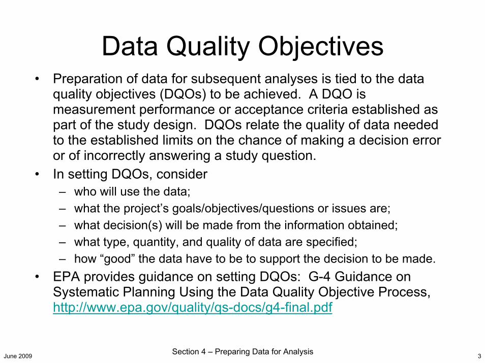
Data Quality Objectives• Preparation of data for subsequent analyses is tied to the data
quality objectives (DQOs) to be achieved. A DQO is measurement performance or acceptance criteria established as part of the study design. DQOs relate the quality of data needed to the established limits on the chance of making a decision error or of incorrectly answering a study question.
• In setting DQOs, consider– who will use the data;– what the project’s goals/objectives/questions or issues are;– what decision(s) will be made from the information obtained;– what type, quantity, and quality of data are specified;– how “good” the data have to be to support the decision to be made.
• EPA provides guidance on setting DQOs: G-4 Guidance on Systematic Planning Using the Data Quality Objective Process, http://www.epa.gov/quality/qs-docs/g4-final.pdf
June 2009 Section 4 – Preparing Data for Analysis 4
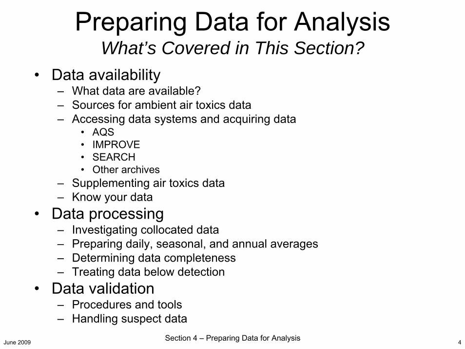
Preparing Data for Analysis What’s Covered in This Section?
• Data availability– What data are available?– Sources for ambient air toxics data– Accessing data systems and acquiring data
• AQS• IMPROVE• SEARCH• Other archives
– Supplementing air toxics data– Know your data
• Data processing– Investigating collocated data– Preparing daily, seasonal, and annual averages– Determining data completeness– Treating data below detection
• Data validation – Procedures and tools– Handling suspect data

June 2009 Section 4 – Preparing Data for Analysis 5
What Data Are Available?Air Toxics Overview
• Air toxics ambient monitoring data is typically collected in three major durations (1-hr, 3-hr, 24-hr)
• Sampling frequencies vary from subdaily, daily, 1-in-3-day,1-in-6-day, to 1-in-12-day
• Some sites have operated as long-term (multiple year) sites while others may report data for a short study only (e.g., a week or two).
• Data can be reported in a range of units. For analyses, consistency in units is essential.
• For data to be useful, a minimum of monitor locations, concentration units, method codes, and parameter names is required. Sampling frequency information is also desirable.
• Keep in mind: Air toxics measurements are primarily captured in urban areas as shown in the figures. VOC* measurements, for example, are typically made in higher population and higher population density areas relative to all counties in the United States.
Plot prepared in SYSTAT using 2000 census and locations of air toxics monitors in 2003-2005.
* VOC: Volatile Organic Compound
0
0.1
0.2
0.3
0.4
0.5
0.6
0.7
0.8
0.9
1
100 1000 10000 100000 1000000 10000000
Population
Frac
tion
of c
ount
ies
US countiesCounties with metals measurementsCounties with VOC measurements
Median county population The subsets of counties with metals or VOC measurements have median populations that are at the upper end of the distribution compared to all US counties.
0.875
0.939
305,000147,00025,000
June 2009 Section 4 – Preparing Data for Analysis 6
What Data Are Available?Sources for Ambient Air Toxics Data
Air toxics data are mostly obtained from federal, state, local and tribal monitoring agencies and are listed here:• EPA’s Air Quality System (AQS) • IMPROVE1 speciated PM2.5 data can be downloaded from VIEWS2
web site, http://vista.cira.colostate.edu/views/• SEARCH3 speciated PM2.5 data can be downloaded from
Atmospheric Research Analysis web site, http://www.atmospheric-research.com/public/index.html
• Air Quality Archive (AQA) (1990-2005) developed during Phase V national air toxics analysis project; includes legacy air toxics archive data (data posted here http://www.epa.gov/ttn/amtic/toxdat.html)
• Local, state and tribal air quality agency databases (i.e., some data are not yet submitted to AQS)
1 IMPROVE = Interagency Monitoring of Protected Visual Environments2 VIEWS = Visibility Information Exchange Web System3 SEARCH = SouthEastern Aerosol Research and Characterization Study
June 2009 Section 4 – Preparing Data for Analysis 7
AQS DataOverview
• AQS is the EPA’s principal data repository, containing the most complete set of toxics (and other) data available.
• To obtain the massive data set required for the national analysis, AQS was accessed via the Intranet with a user ID obtained from EPA.
– AMP501 request provides raw data in R-2 format.• Data are available from 1995 to the present in AQS.• Annual air toxics data are required to be submitted to AQS within 180 days of end of
Q4, i.e., 2007 data would be entered by July 2008.• Archived AMP501 data prior to 1995 were requested directly from EPA.
– Data from AQS are provided in a pipe-delimited format that needs to be transformed and processed.
• For the national assessment, SQL server was used to process data.• Publicly available VOCDat can be used to process data from one site at a time
(http://vocdat.sonomatech.com/).• Some data, such as criteria pollutant summaries, are available for
download without a user ID; most air toxics are not yet available this way. • Find additional information about AQS at
http://www.epa.gov/ttnmain1/airs/airsaqs/• The AQS Discoverer site may be used to retrieve data:
http://www.epa.gov/ttn/airs/airsaqs/aqsdiscover/

June 2009 Section 4 – Preparing Data for Analysis 8
AQS DataCodes
• AQS uses a variety of codes to simplify and condense information in the R-2 output file.
• Key Codes– AQS site code; identifies a particular monitoring site.– AQS parameter code; identifies the pollutant measured. – AQS parameter occurrence code (POC); distinguishes among monitors for the
same pollutant at the same site. – AQS method code; unique for each combination of sample collection and
analysis.• Each code contains additional metadata which would be unnecessarily
repetitive if included in the R-2 file. – For example, default method detection limits MDLs) are not provided in the
R-2 file. This information must be looked up on the AQS website (below) using the method query tool. Alternate MDLs, on the other hand, are included in the R-2 file since they are unique to each record.
• Descriptions of codes and additional metadata can be found at http://www.epa.gov/ttn/airs/airsaqs/manuals/codedescs.htm.
June 2009 Section 4 – Preparing Data for Analysis 9
Other Data Archives (1 of 2)
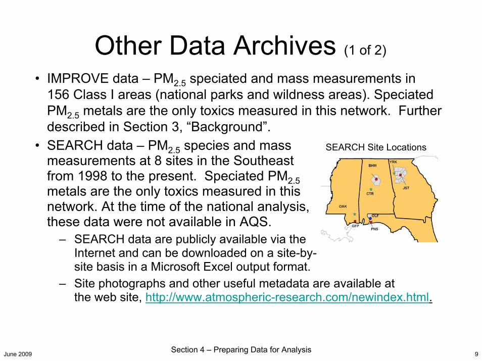
• IMPROVE data – PM2.5 speciated and mass measurements in 156 Class I areas (national parks and wildness areas). SpeciatedPM2.5 metals are the only toxics measured in this network. Further described in Section 3, “Background”.
• SEARCH data – PM2.5 species and mass measurements at 8 sites in the Southeast from 1998 to the present. Speciated PM2.5metals are the only toxics measured in this network. At the time of the national analysis, these data were not available in AQS.
– SEARCH data are publicly available via the Internet and can be downloaded on a site-by-site basis in a Microsoft Excel output format.
– Site photographs and other useful metadata are available at the web site, http://www.atmospheric-research.com/newindex.html.
SEARCH Site Locations
June 2009 Section 4 – Preparing Data for Analysis 10
Other Data Archives (2 of 2)
• As part of several projects, an air quality archive (AQA) was developed as an analysis-ready database that includes data from AQS (1990-2005), IMPROVE and SEARCH data, and data from the legacy air toxics archive.
• This national level database contains nearly 1 billion raw data records, 27 million raw toxics records, and complete validated and temporally aggregated data sets.
• Key data summaries have been posted http://www.epa.gov/ttn/amtic/toxdat.html:– 24-hour CSV Files (very large file) – Monthly CSV Files – Quarterly CSV Files – Annual Average CSV Files – SAS Files (all data, very large file)
• Note: CSV files are comma separated files suitable for importing into spreadsheets or databases. These files are too large to fit into Microsoft Excel spreadsheets but will fit into Microsoft Access. The SAS files are for use with the SAS Statistical Software package.
June 2009 Section 4 – Preparing Data for Analysis 11
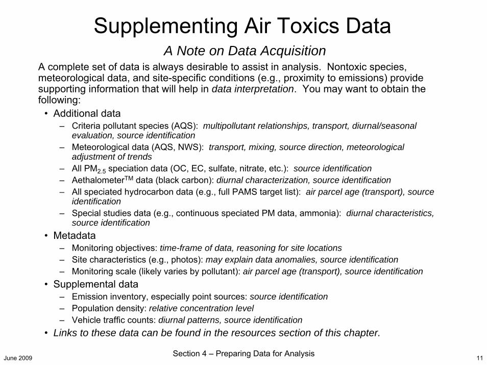
Supplementing Air Toxics DataA Note on Data Acquisition
A complete set of data is always desirable to assist in analysis. Nontoxic species, meteorological data, and site-specific conditions (e.g., proximity to emissions) provide supporting information that will help in data interpretation. You may want to obtain the following:
• Additional data– Criteria pollutant species (AQS): multipollutant relationships, transport, diurnal/seasonal
evaluation, source identification– Meteorological data (AQS, NWS): transport, mixing, source direction, meteorological
adjustment of trends– All PM2.5 speciation data (OC, EC, sulfate, nitrate, etc.): source identification– AethalometerTM data (black carbon): diurnal characterization, source identification– All speciated hydrocarbon data (e.g., full PAMS target list): air parcel age (transport), source
identification– Special studies data (e.g., continuous speciated PM data, ammonia): diurnal characteristics,
source identification• Metadata
– Monitoring objectives: time-frame of data, reasoning for site locations– Site characteristics (e.g., photos): may explain data anomalies, source identification– Monitoring scale (likely varies by pollutant): air parcel age (transport), source identification
• Supplemental data – Emission inventory, especially point sources: source identification– Population density: relative concentration level– Vehicle traffic counts: diurnal patterns, source identification
• Links to these data can be found in the resources section of this chapter.
June 2009 Section 4 – Preparing Data for Analysis 12
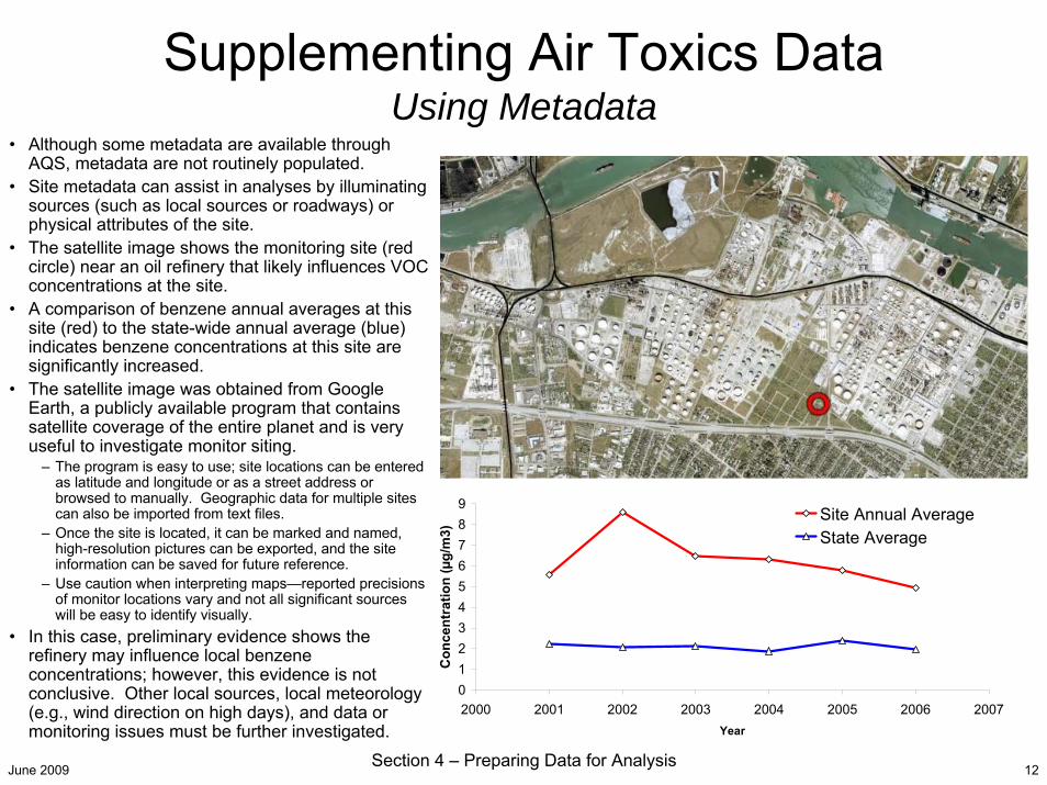
Supplementing Air Toxics DataUsing Metadata
• Although some metadata are available through AQS, metadata are not routinely populated.
• Site metadata can assist in analyses by illuminating sources (such as local sources or roadways) or physical attributes of the site.
• The satellite image shows the monitoring site (red circle) near an oil refinery that likely influences VOC concentrations at the site.
• A comparison of benzene annual averages at this site (red) to the state-wide annual average (blue) indicates benzene concentrations at this site are significantly increased.
• The satellite image was obtained from Google Earth, a publicly available program that contains satellite coverage of the entire planet and is very useful to investigate monitor siting.
– The program is easy to use; site locations can be entered as latitude and longitude or as a street address or browsed to manually. Geographic data for multiple sites can also be imported from text files.
– Once the site is located, it can be marked and named, high-resolution pictures can be exported, and the site information can be saved for future reference.
– Use caution when interpreting maps—reported precisions of monitor locations vary and not all significant sources will be easy to identify visually.
• In this case, preliminary evidence shows the refinery may influence local benzene concentrations; however, this evidence is not conclusive. Other local sources, local meteorology (e.g., wind direction on high days), and data or monitoring issues must be further investigated.
0123456789
2000 2001 2002 2003 2004 2005 2006 2007Year
Con
cent
ratio
n (µ
g/m
3)
Site Annual AverageState Average
June 2009 Section 4 – Preparing Data for Analysis 13
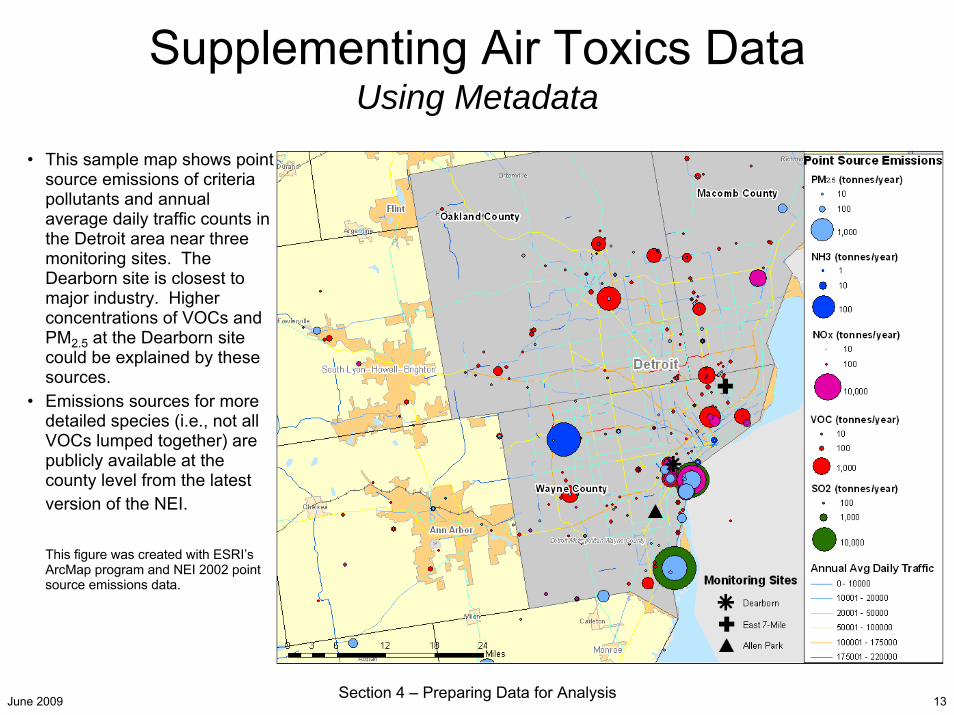
• This sample map shows point source emissions of criteria pollutants and annual average daily traffic counts in the Detroit area near three monitoring sites. The Dearborn site is closest to major industry. Higher concentrations of VOCs and PM2.5 at the Dearborn site could be explained by these sources.
• Emissions sources for more detailed species (i.e., not all VOCs lumped together) are publicly available at the county level from the latest version of the NEI.
This figure was created with ESRI’s ArcMap program and NEI 2002 point source emissions data.
Supplementing Air Toxics DataUsing Metadata

June 2009 Section 4 – Preparing Data for Analysis 14
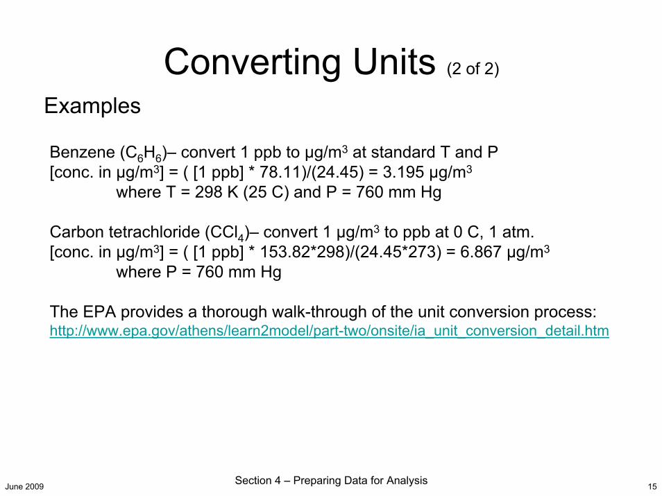
Converting Units (1 of 2)
• Frequently used units for gaseous air toxics include μg/m3, parts per billion (ppb), and parts per billion carbon (ppbC).
• The preferred units for risk assessment are μg/m3. The data are not always delivered or reported in these units.
• Useful equations for converting data units:[conc. in μg/m3] = ( [conc. in ppb] * MW * 298 * P )/(24.45 * T * 760 ) [conc. in ppb] = ([conc. in μg/m3] * 24.45 * T * 760 )/( MW * 298 * P ) ppbC = ppb x (# of carbons in the molecule)
where: MW = molecular weight of compound [g/mol]P = absolute pressure of air [mm Hg]; 1 atm = 760 mm HgT = temperature of air [K]; 298 K is standard
June 2009 Section 4 – Preparing Data for Analysis 15
Converting Units (2 of 2)
Examples
Benzene (C6H6)– convert 1 ppb to μg/m3 at standard T and P[conc. in μg/m3] = ( [1 ppb] * 78.11)/(24.45) = 3.195 μg/m3
where T = 298 K (25 C) and P = 760 mm Hg
Carbon tetrachloride (CCl4)– convert 1 μg/m3 to ppb at 0 C, 1 atm.[conc. in μg/m3] = ( [1 ppb] * 153.82*298)/(24.45*273) = 6.867 μg/m3
where P = 760 mm Hg
The EPA provides a thorough walk-through of the unit conversion process: http://www.epa.gov/athens/learn2model/part-two/onsite/ia_unit_conversion_detail.htm
June 2009 Section 4 – Preparing Data for Analysis 16
Know Your Data Overview
• Before beginning data validation, it helps to know the typical patterns in an air toxics data set. Having this knowledge helps the analyst set expectations for data patterns and identify data anomalies. Diurnal and seasonal patterns help analysts understand possible impacts on data aggregations when some data are missing.
• Using the power of the central tendencies in a large national data set, typical air toxics relationships are provided. Patterns at individual sites may differ from the typical examples shown— understanding why there are differences becomes part of the data validation and data analysis steps.
• EPA has developed tabulated dose-response assessments for use in risk assessment of hazardous air pollutants. The information can be found in two tables at this website: http://www.epa.gov/ttn/atw/toxsource/summary.html. One table presents values for long-term (chronic) inhalation and oral exposures and the other presents short-term (acute) inhalation exposures. Note that these tables are updated periodically to reflect the most recent information; revisions can make a significant impact on risk screening assessments.

June 2009 Section 4 – Preparing Data for Analysis 17
Know Your DataTypical Air Toxics Relationships: Seasonal Trends
Example Seasonal Patterns
The plot shows an example seasonal pattern for carbon tetrachloride, benzene, and manganese PM2.5 at a national level. The figure was produced using Microsoft Excel.
Jan, Feb, Mar April, May, June July, Aug, Sep Oct, Nov, Dec
Season
Nor
mal
ized
Con
cent
ratio
nsCarbon tetrachloride Benzene Manganese PM2.5
Warm season peak
Cool season peak
Warm
Cool
Invariant
Carbon tetrachloride Benzene Manganese PM2.5
• Pollutants that typically correlate well– Acetaldehyde and formaldehyde, similar
sources and reactivity– Benzene and 1,3-butadiene, especially at
locations influenced by mobile source emissions– Toluene, benzene, and ethylbenzene
• Toluene concentrations are typically higher than benzene concentrations
• Toluene and ethylbenzene typically correlate well
• National seasonal patterns– Warm season peak
• Formaldehyde• Acetaldehyde• Chloroform• Manganese PM2.5
– Cool season peak• Benzene• 1,3-butadiene• Hexane• Chlorine PM2.5 (especially at locations where
roads are salted in winter)– Invariant, carbon tetrachloride
June 2009 Section 4 – Preparing Data for Analysis 18
0 1 2 3 4 5 6 7 8 9 10 11 12 13 14 15 16 17 18 19 20 21 22 23Hour
Nor
mal
ized
con
cent
ratio
ns
Benzene Methylene chloride Carbon Tetrachloride Formaldehyde
Rush hour peak
Nighttime peak
Photo-chemical peakMidday Peak
Invariant
Nighttime Peak
Morning Peak
Example Diurnal Patterns
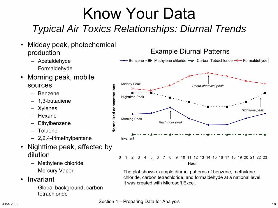
The plot shows example diurnal patterns of benzene, methylene chloride, carbon tetrachloride, and formaldehyde at a national level. It was created with Microsoft Excel.
• Midday peak, photochemical production
– Acetaldehyde – Formaldehyde
• Morning peak, mobile sources
– Benzene– 1,3-butadiene– Xylenes– Hexane– Ethylbenzene– Toluene– 2,2,4-trimethylpentane
• Nighttime peak, affected by dilution
– Methylene chloride– Mercury Vapor
• Invariant– Global background, carbon
tetrachloride
Know Your DataTypical Air Toxics Relationships: Diurnal Trends
June 2009 Section 4 – Preparing Data for Analysis 19
Collocated DataOverview
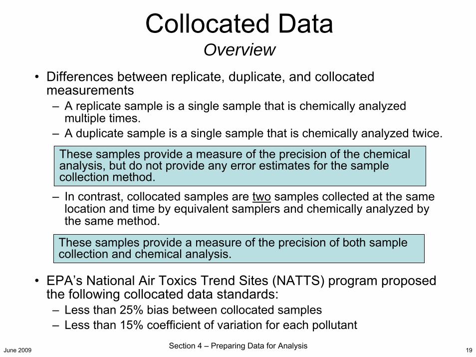
• Differences between replicate, duplicate, and collocated measurements– A replicate sample is a single sample that is chemically analyzed
multiple times. – A duplicate sample is a single sample that is chemically analyzed twice.
– In contrast, collocated samples are two samples collected at the same location and time by equivalent samplers and chemically analyzed by the same method.
• EPA’s National Air Toxics Trend Sites (NATTS) program proposed the following collocated data standards:– Less than 25% bias between collocated samples – Less than 15% coefficient of variation for each pollutant
These samples provide a measure of the precision of the chemicalanalysis, but do not provide any error estimates for the sample collection method.
These samples provide a measure of the precision of both sample collection and chemical analysis.
June 2009 Section 4 – Preparing Data for Analysis 20
Collocated DataHandling Collocated Data
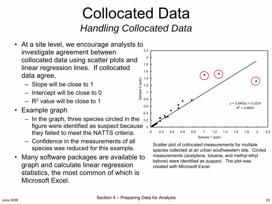
• At a site level, we encourage analysts to investigate agreement between collocated data using scatter plots and linear regression lines. If collocated data agree,
– Slope will be close to 1– Intercept will be close to 0– R2 value will be close to 1
• Example graph– In the graph, three species circled in the
figure were identified as suspect because they failed to meet the NATTS criteria.
– Confidence in the measurements of all species was reduced for this example.
• Many software packages are available to graph and calculate linear regression statistics, the most common of which is Microsoft Excel.
y = 0.9452x + 0.0224R2 = 0.8853
0
0.2
0.4
0.6
0.8
1
1.2
1.4
1.6
1.8
2
2.2
0 0.2 0.4 0.6 0.8 1 1.2 1.4 1.6 1.8 2 2.2
Sample 1 (ppb)S
ampl
e 2
(ppb
)Scatter plot of collocated measurements for multiple species collected at an urban southwestern site. Circled measurements (acetylene, toluene, and methyl ethyl ketone) were identified as suspect. The plot was created with Microsoft Excel.
June 2009 Section 4 – Preparing Data for Analysis 21
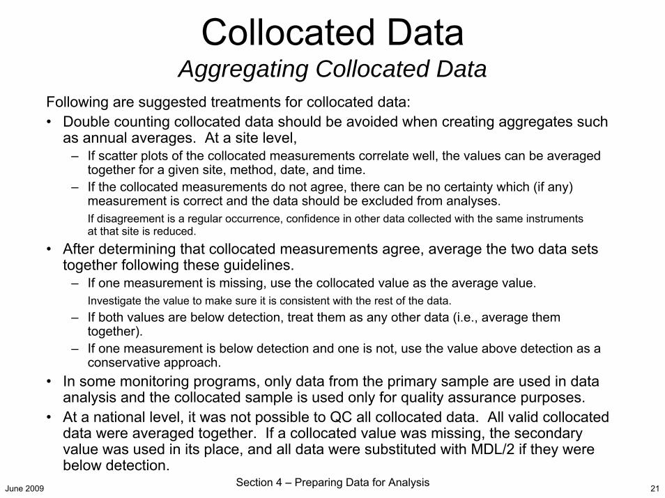
Following are suggested treatments for collocated data:• Double counting collocated data should be avoided when creating aggregates such
as annual averages. At a site level,– If scatter plots of the collocated measurements correlate well, the values can be averaged
together for a given site, method, date, and time.– If the collocated measurements do not agree, there can be no certainty which (if any)
measurement is correct and the data should be excluded from analyses.If disagreement is a regular occurrence, confidence in other data collected with the same instruments at that site is reduced.
• After determining that collocated measurements agree, average the two data sets together following these guidelines.
– If one measurement is missing, use the collocated value as the average value.Investigate the value to make sure it is consistent with the rest of the data.
– If both values are below detection, treat them as any other data (i.e., average them together).
– If one measurement is below detection and one is not, use the value above detection as a conservative approach.
• In some monitoring programs, only data from the primary sample are used in data analysis and the collocated sample is used only for quality assurance purposes.
• At a national level, it was not possible to QC all collocated data. All valid collocated data were averaged together. If a collocated value was missing, the secondary value was used in its place, and all data were substituted with MDL/2 if they were below detection.
Collocated DataAggregating Collocated Data
June 2009 Section 4 – Preparing Data for Analysis 22
Data CompletenessOverview
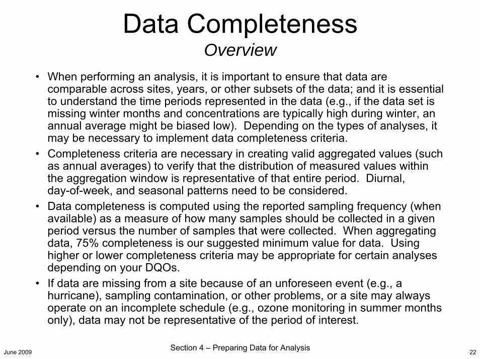
• When performing an analysis, it is important to ensure that data are comparable across sites, years, or other subsets of the data; and it is essential to understand the time periods represented in the data (e.g., if the data set is missing winter months and concentrations are typically high during winter, an annual average might be biased low). Depending on the types of analyses, it may be necessary to implement data completeness criteria.
• Completeness criteria are necessary in creating valid aggregated values (such as annual averages) to verify that the distribution of measured values within the aggregation window is representative of that entire period. Diurnal, day-of-week, and seasonal patterns need to be considered.
• Data completeness is computed using the reported sampling frequency (when available) as a measure of how many samples should be collected in a given period versus the number of samples that were collected. When aggregating data, 75% completeness is our suggested minimum value for data. Using higher or lower completeness criteria may be appropriate for certain analyses depending on your DQOs.
• If data are missing from a site because of an unforeseen event (e.g., a hurricane), sampling contamination, or other problems, or a site may always operate on an incomplete schedule (e.g., ozone monitoring in summer months only), data may not be representative of the period of interest.

June 2009 Section 4 – Preparing Data for Analysis 23
Data CompletenessInterpreting Notched Box Plots
• Notched box whisker plots are useful for showing the central trends of the data (i.e., the median) while also showing variability (i.e., the box and whiskers).
• Definitions provided are for plots prepared using SYSTAT software; other software may have different definitions.
25th percentile
75th percentile
0
100
200
300
Mea
sure
Outliers
Notcharoundmedian
Median
95 % C.I.
95 % C.I.
0
5
10
15
20
Mea
sure
75th percentile
Median
25th percentile
Box(Interquartile
range)
Whisker
Outliers
Data within 1.5*IR
Data within 3*IR
Whisker
Data > 3*IR
June 2009 Section 4 – Preparing Data for Analysis 24
Data CompletenessExample Effect of Aggregating Incomplete Data
Figures were created in SYSTAT
Benzene
0 1 2 3 4 5 6 7 8 9 10 11 12 13MONTH
0
1
2
3
Con
cent
ratio
n (u
g/m
3)
0 1 2 3 4 5 6 7 8 9 10 11 12 13MONTH
0
1
2
3
Con
cent
ratio
n (u
g/m
3)
WinterSummer
SEASON
3)
3)
Co n
cent
rat io
n (u
g/m
Co n
cent
rat io
n (u
g/m
1996 1998 2000 2002 2004 2006YEAR
0
1
2
3
4
Con
cent
rati o
n (u
g/m
3)
1996 1998 2000 2002 2004 20060
1
2
3
4
WinterSummer
Average of All Data
3)
3)
Co n
cent
rat io
n (u
g/m
Co n
cent
rat io
n (u
g/m
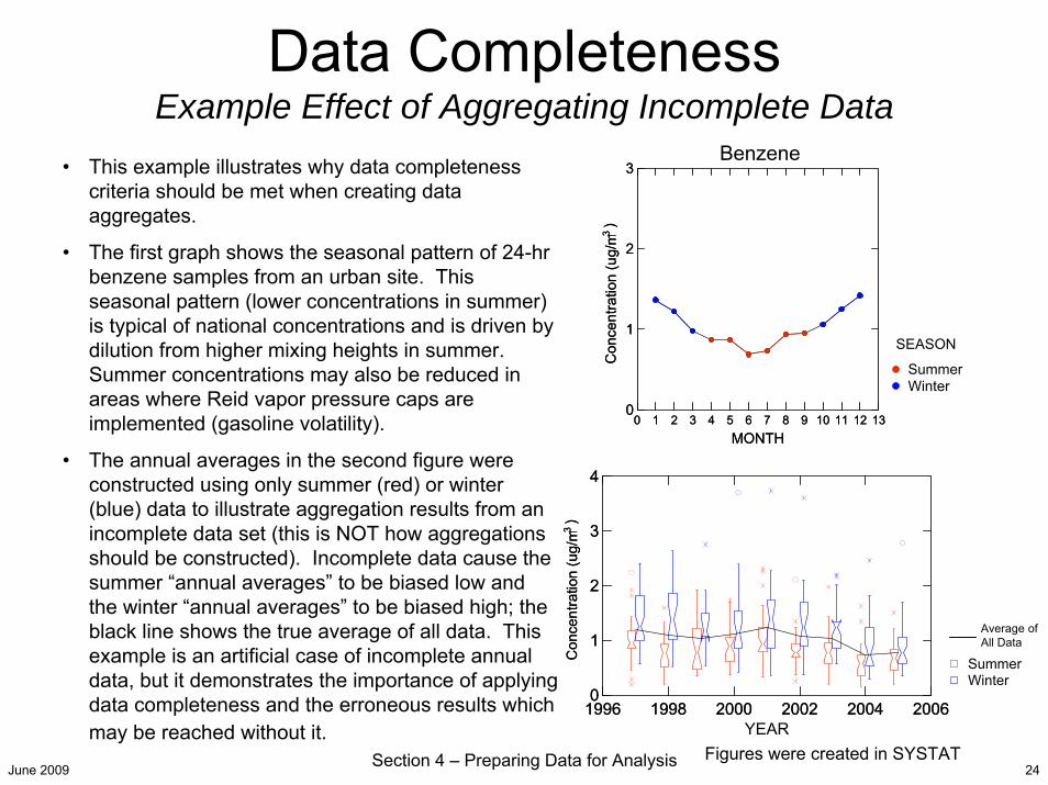
• This example illustrates why data completeness criteria should be met when creating data aggregates.
• The first graph shows the seasonal pattern of 24-hr benzene samples from an urban site. This seasonal pattern (lower concentrations in summer) is typical of national concentrations and is driven by dilution from higher mixing heights in summer. Summer concentrations may also be reduced in areas where Reid vapor pressure caps are implemented (gasoline volatility).
• The annual averages in the second figure were constructed using only summer (red) or winter (blue) data to illustrate aggregation results from an incomplete data set (this is NOT how aggregations should be constructed). Incomplete data cause the summer “annual averages” to be biased low and the winter “annual averages” to be biased high; the black line shows the true average of all data. This example is an artificial case of incomplete annual data, but it demonstrates the importance of applying data completeness and the erroneous results which may be reached without it.
June 2009 Section 4 – Preparing Data for Analysis 25
Data AggregationCreating Valid 24-hr Averages
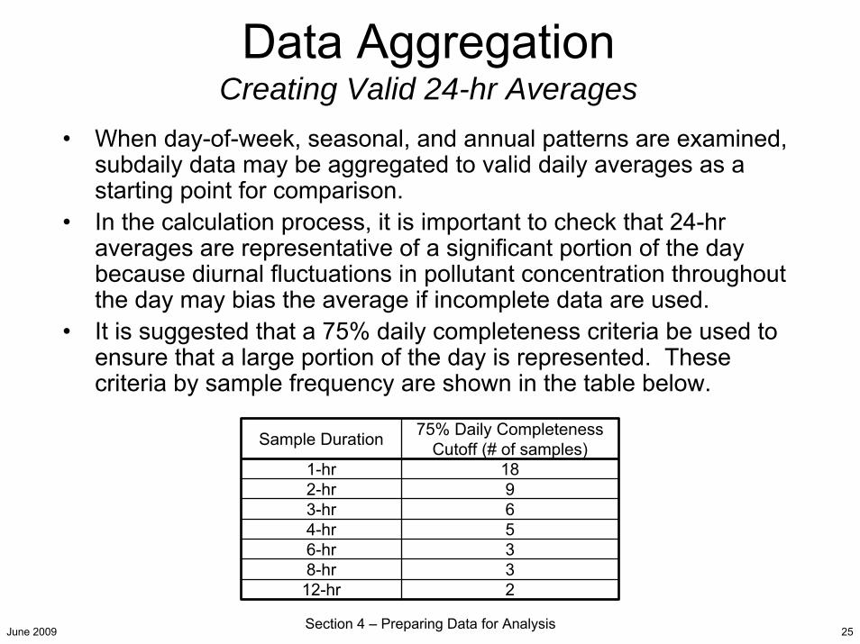
• When day-of-week, seasonal, and annual patterns are examined, subdaily data may be aggregated to valid daily averages as a starting point for comparison.
• In the calculation process, it is important to check that 24-hr averages are representative of a significant portion of the day because diurnal fluctuations in pollutant concentration throughout the day may bias the average if incomplete data are used.
• It is suggested that a 75% daily completeness criteria be used to ensure that a large portion of the day is represented. These criteria by sample frequency are shown in the table below.
Sample Duration 75% Daily Completeness Cutoff (# of samples)
1-hr 182-hr 93-hr 64-hr 56-hr 38-hr 3
12-hr 2
June 2009 Section 4 – Preparing Data for Analysis 26
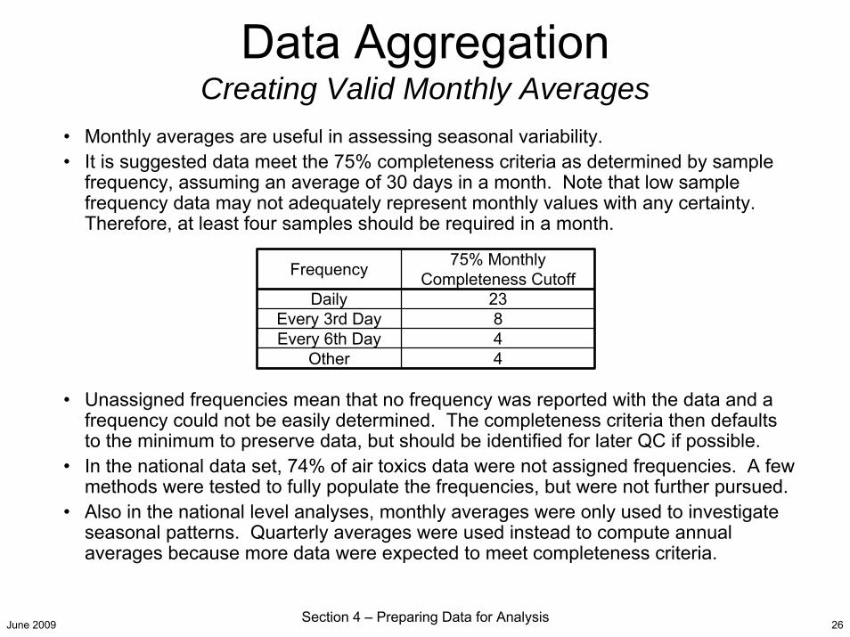
Data AggregationCreating Valid Monthly Averages
• Monthly averages are useful in assessing seasonal variability.• It is suggested data meet the 75% completeness criteria as determined by sample
frequency, assuming an average of 30 days in a month. Note that low sample frequency data may not adequately represent monthly values with any certainty. Therefore, at least four samples should be required in a month.
• Unassigned frequencies mean that no frequency was reported with the data and a frequency could not be easily determined. The completeness criteria then defaults to the minimum to preserve data, but should be identified for later QC if possible.
• In the national data set, 74% of air toxics data were not assigned frequencies. A few methods were tested to fully populate the frequencies, but were not further pursued.
• Also in the national level analyses, monthly averages were only used to investigate seasonal patterns. Quarterly averages were used instead to compute annual averages because more data were expected to meet completeness criteria.
Frequency 75% Monthly Completeness Cutoff
Daily 23Every 3rd Day 8Every 6th Day 4
Other 4
June 2009 Section 4 – Preparing Data for Analysis 27
Data AggregationCreating Valid Quarterly and Annual Averages
• Annual averages are calculated by first computing valid quarterly averages• Quarterly Averages
– Quarterly averages are calculated from valid 24-hr averages.– 75% of data at the expected daily sampling frequency is suggested for a valid
calendar quarter average, i.e.,
– At least 58 days are suggested between the first and last sample in a quarter to ensure sampling represented the entire quarter.
– Unassigned frequencies mean that no frequency was reported with the data and a frequency could not be easily determined. The completeness criteria then defaults to the minimum to preserve data, but should be identified for later QC if possible.
• Annual Averages – three out of four valid quarterly averages are required.
Frequency 75% Quarterly Completeness Cutoff
Daily 68
Every 3rd Day 24
Every 6th Day 12
Every 12th Day 6
Unassigned 6

June 2009 Section 4 – Preparing Data for Analysis 28
Method Detection LimitsOverview
• The EPA Code of Federal Regulations (CFR) defines the MDL as “The minimum concentration of a substance that can be measured and reported with 99% confidence that the analyte concentration is greater than zero and is determined from analysis of a sample in a given matrix containing the analyte”.
• The purpose of an MDL is to discriminate against false positives. Values reported below the MDL have much higher uncertainty but can provide insight into the lower concentration distribution (i.e., are most values closer to the MDL or to zero?).
In the illustration, normally distributed results from a measured value of zero yields a 99% confidence value (3σ) at 3 ppb, which would be used as the MDL in this case. There is >99% confidence that values above 3 ppb are not false positives.
-3 -2 -1 0 1 2 3 4 5Concentration (ppb)
MDL TrueValue
Environmental Protection Agency, 1982
June 2009 Section 4 – Preparing Data for Analysis 29
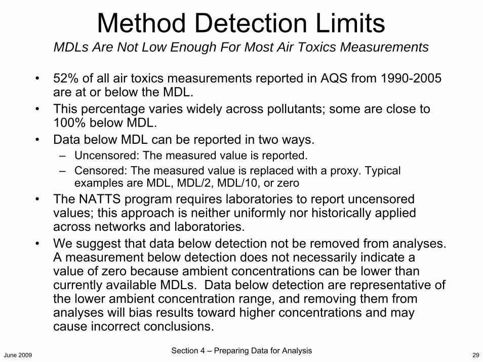
• 52% of all air toxics measurements reported in AQS from 1990-2005 are at or below the MDL.
• This percentage varies widely across pollutants; some are close to 100% below MDL.
• Data below MDL can be reported in two ways.– Uncensored: The measured value is reported. – Censored: The measured value is replaced with a proxy. Typical
examples are MDL, MDL/2, MDL/10, or zero• The NATTS program requires laboratories to report uncensored
values; this approach is neither uniformly nor historically applied across networks and laboratories.
• We suggest that data below detection not be removed from analyses. A measurement below detection does not necessarily indicate a value of zero because ambient concentrations can be lower than currently available MDLs. Data below detection are representative of the lower ambient concentration range, and removing them from analyses will bias results toward higher concentrations and may cause incorrect conclusions.
Method Detection LimitsMDLs Are Not Low Enough For Most Air Toxics Measurements
June 2009 Section 4 – Preparing Data for Analysis 30
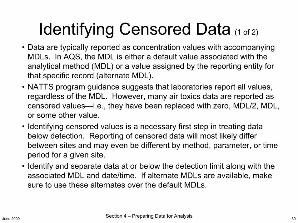
• Data are typically reported as concentration values with accompanying MDLs. In AQS, the MDL is either a default value associated with the analytical method (MDL) or a value assigned by the reporting entity for that specific record (alternate MDL).
• NATTS program guidance suggests that laboratories report all values, regardless of the MDL. However, many air toxics data are reported as censored values—i.e., they have been replaced with zero, MDL/2, MDL, or some other value.
• Identifying censored values is a necessary first step in treating data below detection. Reporting of censored data will most likely differ between sites and may even be different by method, parameter, or time period for a given site.
• Identify and separate data at or below the detection limit along with the associated MDL and date/time. If alternate MDLs are available, make sure to use these alternates over the default MDLs.
Identifying Censored Data (1 of 2)

June 2009 Section 4 – Preparing Data for Analysis 31
Identifying Censored Data (2 of 2)
• Examine the data for obvious substitution. Count the number of times each value at or below detection is reported for a given site, parameter, and method. Are the majority of data reported as the same value (e.g., zero or MDL/2)?
– If data are largely reported as two or more values, investigate the temporal variation of the data. Are there large step changes where reporting methods or MDLs have changed?
– Do the duplicate values indicate a typical censoring method (e.g., MDL/2, MDL/10)?– Alternate MDLs may be different for each sample run causing a distribution of values if
MDL/x substitutions were used. That values below MDL are not all the same does not mean they are not censored.
• Check for MDL/X substitution.– Make a scatter plot of the value vs. MDL to see if the data fall on a straight line. – If the data form a straight line, the slope of the regression line will indicate the value by
which the MDL has been divided. • Is the value a reasonable number that would be used for MDL substitution (e.g., 1,2,5
or 10)?– If the data have been formatted, processed, or converted, ratios may not be exactly the same
due to rounding differences; the distribution should be close to a straight line and centered around a single integer if MDL/x substitutions have been made.
– If a bifurcated pattern is observed, the substitution method may have changed over time. Plot a time series of the ratios and look for step changes.
• The distribution of the ratios should be highly variable if the data are not censored.

June 2009 Section 4 – Preparing Data for Analysis 32
Identifying Censored DataExample
• The data shown in the table are values for a given air toxic below detection in a selected year.
• The reported data, at first glance, appear to be “real”concentrations (e.g., the histogram shows a distribution of concentrations).
• However, the ratio of MDL to reported concentration equals 2 (with very small deviations likely due to unit conversions). The relationship is also visible in a scatter plot as shown here.
• Therefore, in this example, the reported concentrations have been substituted with MDL/2.
Reported Concentration
(µg/m3)MDL (µg/m3)
0.19161 0.382370.20438 0.408340.22141 0.442830.38748 0.779210.40451 0.813270.37896 0.757920.17032 0.344040.18309 0.361930.27251 0.545020.31935 0.642950.31083 0.621660.29380 0.587600.32361 0.651470.26825 0.532250.27677 0.553540.31509 0.630180.25548 0.515210.32786 0.655730.27677 0.553540.25548 0.515210.25548 0.515210.25548 0.515210.29380 0.587600.31083 0.621660.1 0.2 0.3 0.4 0.5
CONC
0
5
10
15
Cou
nt
0.0
0.1
0.2
0.3
0.4
0.5
0.6
Proportion per B
ar
y = 2.0x - 0.0R2 = 1.0
0.1
0.2
0.3
0.4
0.3 0.5 0.7 0.9
Rep
orte
d C
once
ntra
tion
(μg/
m3 )
MDL (μg/m3)
June 2009 Section 4 – Preparing Data for Analysis 33
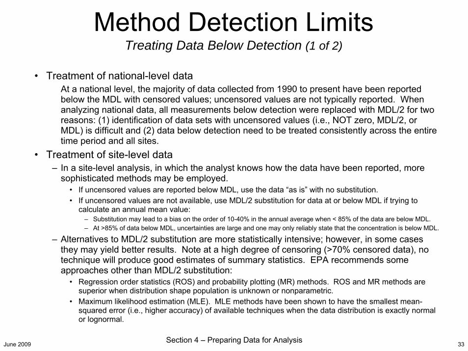
• Treatment of national-level dataAt a national level, the majority of data collected from 1990 to present have been reported below the MDL with censored values; uncensored values are not typically reported. When analyzing national data, all measurements below detection were replaced with MDL/2 for two reasons: (1) identification of data sets with uncensored values (i.e., NOT zero, MDL/2, or MDL) is difficult and (2) data below detection need to be treated consistently across the entire time period and all sites.
• Treatment of site-level data– In a site-level analysis, in which the analyst knows how the data have been reported, more
sophisticated methods may be employed. • If uncensored values are reported below MDL, use the data “as is” with no substitution.• If uncensored values are not available, use MDL/2 substitution for data at or below MDL if trying to
calculate an annual mean value:– Substitution may lead to a bias on the order of 10-40% in the annual average when < 85% of the data are below MDL. – At >85% of data below MDL, uncertainties are large and one may only reliably state that the concentration is below MDL.
– Alternatives to MDL/2 substitution are more statistically intensive; however, in some cases they may yield better results. Note at a high degree of censoring (>70% censored data), no technique will produce good estimates of summary statistics. EPA recommends some approaches other than MDL/2 substitution:
• Regression order statistics (ROS) and probability plotting (MR) methods. ROS and MR methods are superior when distribution shape population is unknown or nonparametric.
• Maximum likelihood estimation (MLE). MLE methods have been shown to have the smallest mean-squared error (i.e., higher accuracy) of available techniques when the data distribution is exactly normal or lognormal.
Method Detection LimitsTreating Data Below Detection (1 of 2)
June 2009 Section 4 – Preparing Data for Analysis 34
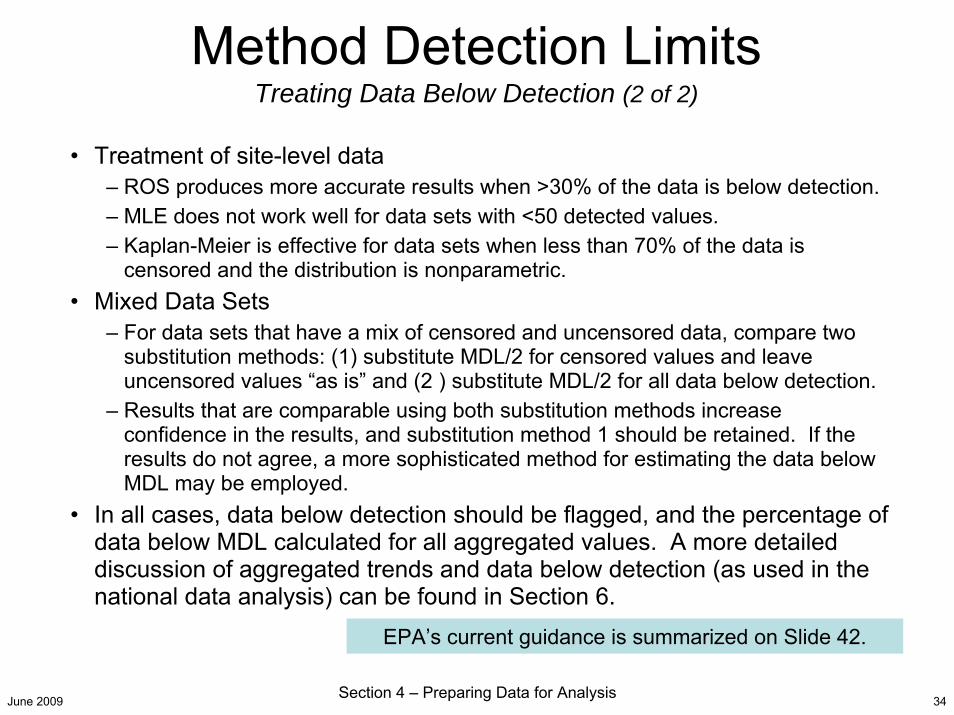
• Treatment of site-level data– ROS produces more accurate results when >30% of the data is below detection. – MLE does not work well for data sets with <50 detected values.– Kaplan-Meier is effective for data sets when less than 70% of the data is
censored and the distribution is nonparametric. • Mixed Data Sets
– For data sets that have a mix of censored and uncensored data, compare two substitution methods: (1) substitute MDL/2 for censored values and leave uncensored values “as is” and (2 ) substitute MDL/2 for all data below detection.
– Results that are comparable using both substitution methods increase confidence in the results, and substitution method 1 should be retained. If the results do not agree, a more sophisticated method for estimating the data below MDL may be employed.
• In all cases, data below detection should be flagged, and the percentage of data below MDL calculated for all aggregated values. A more detailed discussion of aggregated trends and data below detection (as used in the national data analysis) can be found in Section 6.
Method Detection LimitsTreating Data Below Detection (2 of 2)
EPA’s current guidance is summarized on Slide 42.
June 2009 Section 4 – Preparing Data for Analysis 35
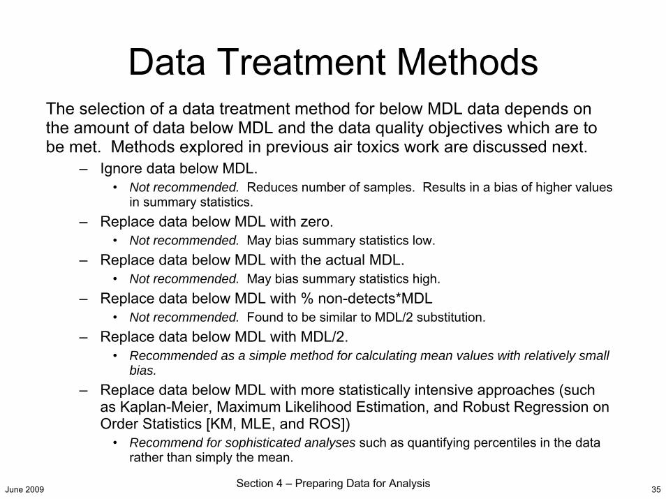
Data Treatment MethodsThe selection of a data treatment method for below MDL data depends on the amount of data below MDL and the data quality objectives which are to be met. Methods explored in previous air toxics work are discussed next.
– Ignore data below MDL.• Not recommended. Reduces number of samples. Results in a bias of higher values
in summary statistics.– Replace data below MDL with zero.
• Not recommended. May bias summary statistics low.– Replace data below MDL with the actual MDL.
• Not recommended. May bias summary statistics high.– Replace data below MDL with % non-detects*MDL
• Not recommended. Found to be similar to MDL/2 substitution.– Replace data below MDL with MDL/2.
• Recommended as a simple method for calculating mean values with relatively small bias.
– Replace data below MDL with more statistically intensive approaches (such as Kaplan-Meier, Maximum Likelihood Estimation, and Robust Regression on Order Statistics [KM, MLE, and ROS])
• Recommend for sophisticated analyses such as quantifying percentiles in the data rather than simply the mean.
June 2009 Section 4 – Preparing Data for Analysis 36
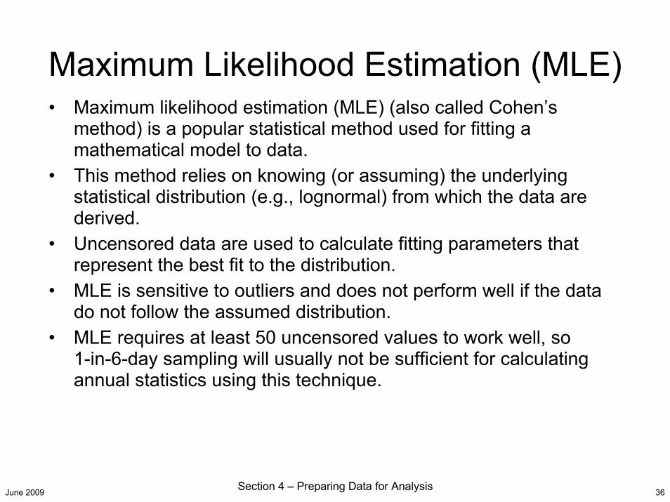
Maximum Likelihood Estimation (MLE)• Maximum likelihood estimation (MLE) (also called Cohen’s
method) is a popular statistical method used for fitting a mathematical model to data.
• This method relies on knowing (or assuming) the underlying statistical distribution (e.g., lognormal) from which the data are derived.
• Uncensored data are used to calculate fitting parameters that represent the best fit to the distribution.
• MLE is sensitive to outliers and does not perform well if the data do not follow the assumed distribution.
• MLE requires at least 50 uncensored values to work well, so 1-in-6-day sampling will usually not be sufficient for calculating annual statistics using this technique.
June 2009 Section 4 – Preparing Data for Analysis 37
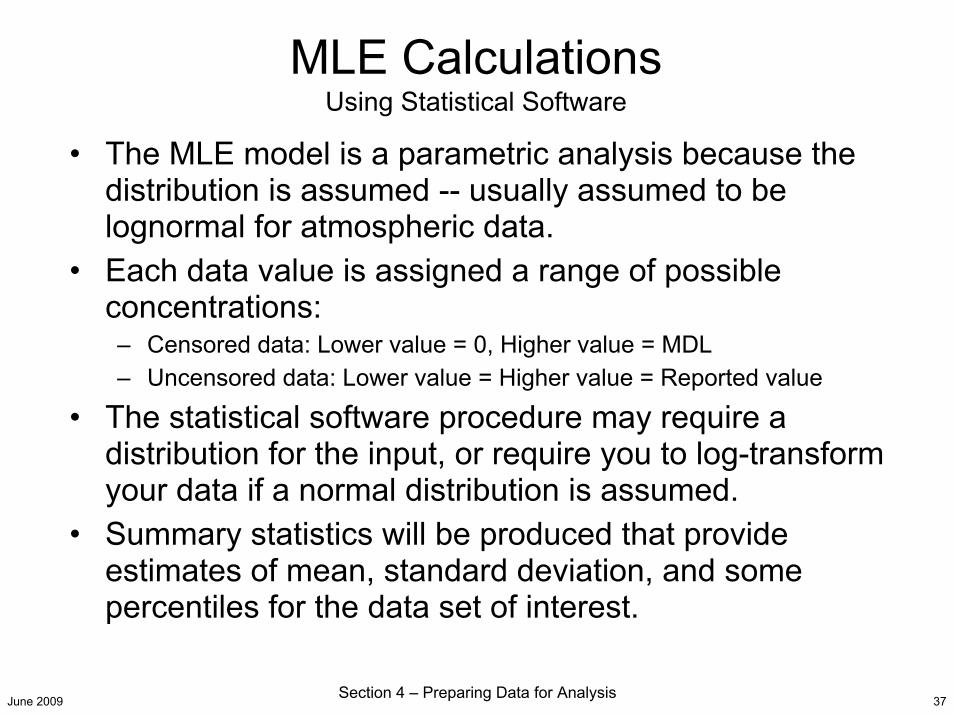
MLE Calculations Using Statistical Software
• The MLE model is a parametric analysis because the distribution is assumed -- usually assumed to be lognormal for atmospheric data.
• Each data value is assigned a range of possible concentrations: – Censored data: Lower value = 0, Higher value = MDL– Uncensored data: Lower value = Higher value = Reported value
• The statistical software procedure may require a distribution for the input, or require you to log-transform your data if a normal distribution is assumed.
• Summary statistics will be produced that provide estimates of mean, standard deviation, and some percentiles for the data set of interest.
June 2009 Section 4 – Preparing Data for Analysis 38
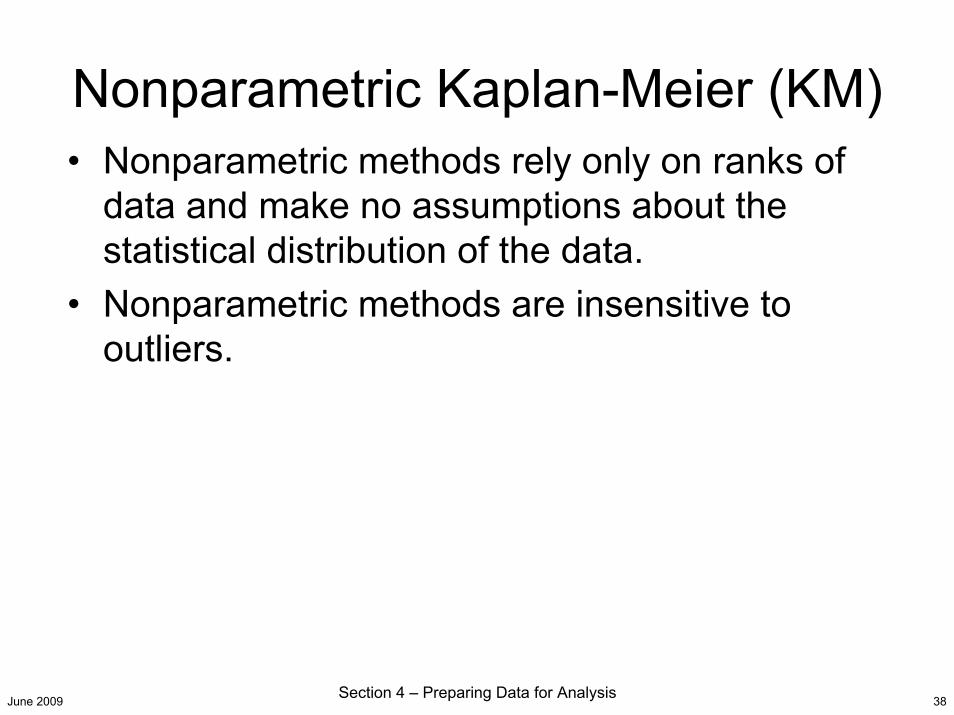
Nonparametric Kaplan-Meier (KM)• Nonparametric methods rely only on ranks of
data and make no assumptions about the statistical distribution of the data.
• Nonparametric methods are insensitive to outliers.
June 2009 Section 4 – Preparing Data for Analysis 39
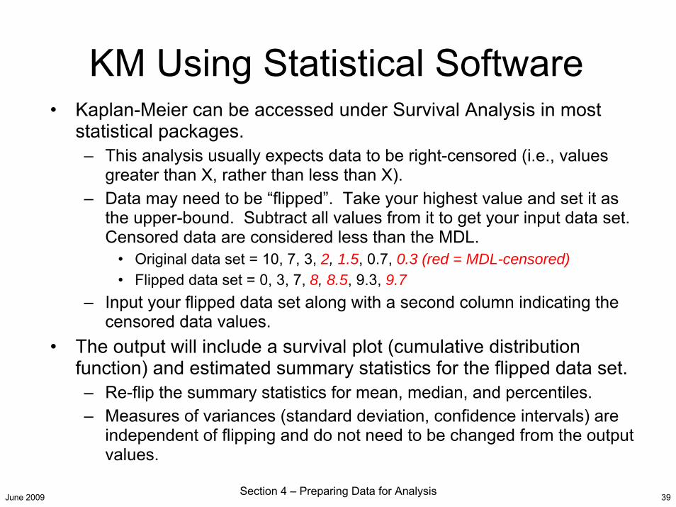
KM Using Statistical Software• Kaplan-Meier can be accessed under Survival Analysis in most
statistical packages.– This analysis usually expects data to be right-censored (i.e., values
greater than X, rather than less than X). – Data may need to be “flipped”. Take your highest value and set it as
the upper-bound. Subtract all values from it to get your input data set. Censored data are considered less than the MDL.
• Original data set = 10, 7, 3, 2, 1.5, 0.7, 0.3 (red = MDL-censored)• Flipped data set = 0, 3, 7, 8, 8.5, 9.3, 9.7
– Input your flipped data set along with a second column indicating the censored data values.
• The output will include a survival plot (cumulative distributionfunction) and estimated summary statistics for the flipped data set. – Re-flip the summary statistics for mean, median, and percentiles.– Measures of variances (standard deviation, confidence intervals) are
independent of flipping and do not need to be changed from the output values.
June 2009 Section 4 – Preparing Data for Analysis 40
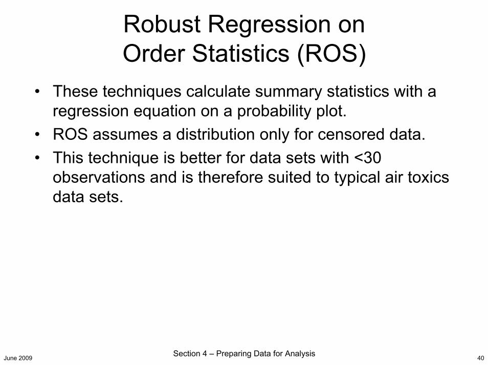
Robust Regression onOrder Statistics (ROS)
• These techniques calculate summary statistics with a regression equation on a probability plot.
• ROS assumes a distribution only for censored data.• This technique is better for data sets with <30
observations and is therefore suited to typical air toxics data sets.
June 2009 Section 4 – Preparing Data for Analysis 41
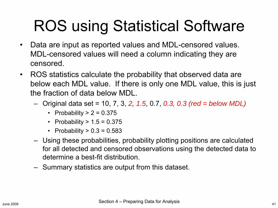
ROS using Statistical Software• Data are input as reported values and MDL-censored values.
MDL-censored values will need a column indicating they are censored.
• ROS statistics calculate the probability that observed data are below each MDL value. If there is only one MDL value, this is just the fraction of data below MDL. – Original data set = 10, 7, 3, 2, 1.5, 0.7, 0.3, 0.3 (red = below MDL)
• Probability > 2 = 0.375• Probability > 1.5 = 0.375• Probability > 0.3 = 0.583
– Using these probabilities, probability plotting positions are calculated for all detected and censored observations using the detected data to determine a best-fit distribution.
– Summary statistics are output from this dataset.
June 2009 Section 4 – Preparing Data for Analysis 42
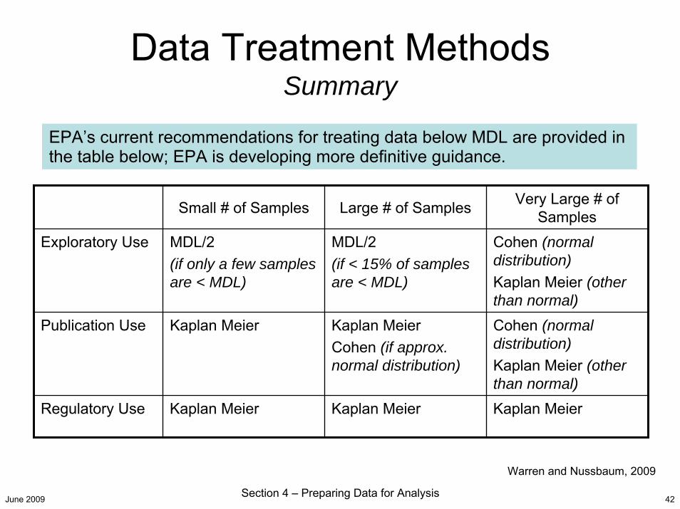
Data Treatment Methods Summary
Small # of Samples Large # of Samples Very Large # of Samples
Exploratory Use MDL/2 (if only a few samples are < MDL)
MDL/2(if < 15% of samples are < MDL)
Cohen (normal distribution)Kaplan Meier (other than normal)
Publication Use Kaplan Meier Kaplan MeierCohen (if approx. normal distribution)
Cohen (normal distribution)Kaplan Meier (other than normal)
Regulatory Use Kaplan Meier Kaplan Meier Kaplan Meier
EPA’s current recommendations for treating data below MDL are provided in the table below; EPA is developing more definitive guidance.
Warren and Nussbaum, 2009
June 2009 Section 4 – Preparing Data for Analysis 43
Data Validation Introduction (1 of 2)
• Data validation is defined as the process of determining the quality and validity of observations.
• The purpose of data validation is to detect and verify any data values that may not represent the actual physical and chemical conditions at the sampling station before the data are used in analysis.
• Validation guidelines are built on knowledge of typical air toxics emissions sources; formation, loss, and transport processes; chemical relationships; and site-specific knowledge.
• The primary objective is to produce a database with values that are of a known quality, an acceptable quality, or a level of uncertainty given the analyses intended to be conducted.
June 2009 Section 4 – Preparing Data for Analysis 44
• The identification of outliers, errors, or biases is typically carried out in several stages or validation levels (U.S. Environmental Protection Agency 1999).
– Level 0: Routine verification that field and laboratory operations were conducted in accordance with standard operating procedures (SOPs) and that initial data processing and reporting were performed in accordance with the SOP (typically the monitoring entity performs this step).
– Level I: Internal consistency tests to identify values in the data that appear atypical when compared to values in the entire data set.
– Level II: Comparisons of current data with historical data (from the same site) to verify consistency over time.
– Level III: Parallel consistency tests with other data sets with possibly similar characteristics (e.g., the same region, period of time, background values, air mass) to identify systematic bias.
• The data analyst performs Level 1 steps, and performs additional validation when other data sets are available.
• Data validation is improved by understanding air toxics emissions, formation, transport, and removal processes. Useful supplementary information in understanding air toxics species (including data sheets and other information about air toxics species) is available (links and examples are provided in the appendix to this section).
• There is no substitute for the local knowledge of monitoring sites; operators or those who have extensive knowledge of the area are a unique resource for data analysts. However, for those not familiar with a site, spatial maps with topography, emissions source, and roadway information are excellent tools for understanding site characteristics.
Data Validation Introduction (2 of 2)
June 2009 Section 4 – Preparing Data for Analysis 45
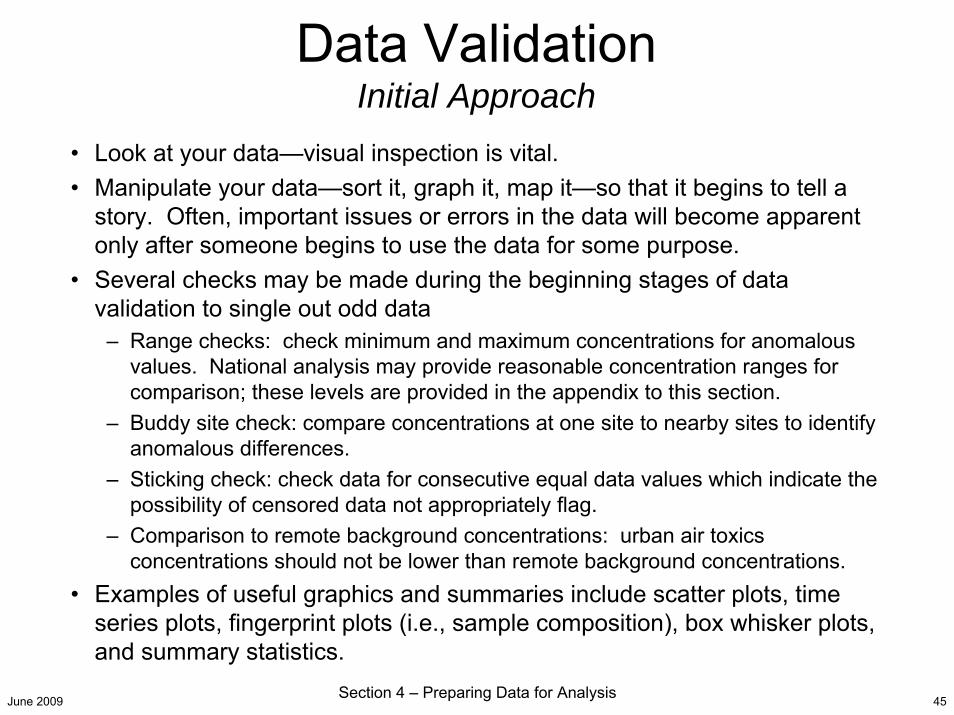
Data ValidationInitial Approach
• Look at your data—visual inspection is vital.• Manipulate your data—sort it, graph it, map it—so that it begins to tell a
story. Often, important issues or errors in the data will become apparent only after someone begins to use the data for some purpose.
• Several checks may be made during the beginning stages of data validation to single out odd data
– Range checks: check minimum and maximum concentrations for anomalous values. National analysis may provide reasonable concentration ranges for comparison; these levels are provided in the appendix to this section.
– Buddy site check: compare concentrations at one site to nearby sites to identify anomalous differences.
– Sticking check: check data for consecutive equal data values which indicate the possibility of censored data not appropriately flag.
– Comparison to remote background concentrations: urban air toxics concentrations should not be lower than remote background concentrations.
• Examples of useful graphics and summaries include scatter plots, time series plots, fingerprint plots (i.e., sample composition), box whisker plots, and summary statistics.
June 2009 Section 4 – Preparing Data for Analysis 46
Things to Consider When Evaluating Your Data
• Levels of other pollutantsA high concentration of benzene may be valid when concentrations of all mobile source air toxics in the sample are also elevated.
• Time of day/yearHigher concentrations of some air toxics are expected in the summer (such as formaldehyde) than in the winter and vice versa for benzene.
• Observations at other sitesHigh concentrations of a pollutant at several sites in an area on the same date may indicate a real emission event.
• Audits and inter-laboratory comparisonsIf data are from differing sources, how well did the concentrations compare between labs? Did audits show some specific “problem” pollutants?
• Site characteristicsHigh concentrations may be expected for a pollutant emitted by a nearby source.
• Unique events (e.g., holiday fireworks)High concentrations of trace metals associated with fireworks are seen around the Fourth of July and New Years Day at many sites.

June 2009 Section 4 – Preparing Data for Analysis 47
• Overall– Proceed from the big picture to the details. For example, proceed from
inspecting species groups to individual species.– Inspect every specie, even to confirm that a specie normally absent
met that expectation.– Know the site topography, prevalent meteorology, and major emissions
sources nearby.• Inspect time series for the following
– Large “jumps” or “dips” in concentrations which may indicate a change in analysis method or MDL.
– Periodicity of peaks. (Is there a pattern? Can the pattern be related to emissions or meteorology?)
– Expected seasonal behavior (e.g., photochemically formed speciesconcentrations usually peak during summer).
– Expected relationships among species (e.g., benzene and toluene typically correlate).
Data ValidationTips and Tricks (1 of 2)
June 2009 Section 4 – Preparing Data for Analysis 48
• To further investigate outliers,– Use wind direction data (e.g., Do outliers occur from a consistent wind
direction?).– Use subsets of data (e.g., inspect high concentration days vs. other
days for differences in meteorology or emissions).– Investigate industrial or agricultural operating schedules, unusual
events, etc. (e.g., Were high metals data associated with a dustevent?).
– Determine local traffic patterns (e.g., When does peak traffic occur? Is there a recreational area or event venue nearby?).
– If no explanation is forthcoming, try contacting the agency thatcollected the data; they may have realized a problem too recently to report it, or your question may alert them to a problem with data collection, analysis, or reporting.
Data ValidationTips and Tricks (2 of 2)
June 2009 Section 4 – Preparing Data for Analysis 49
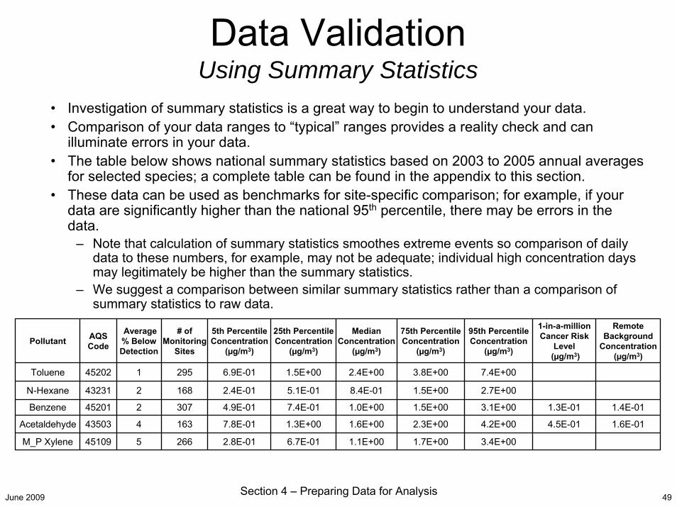
Data ValidationUsing Summary Statistics
• Investigation of summary statistics is a great way to begin to understand your data.• Comparison of your data ranges to “typical” ranges provides a reality check and can
illuminate errors in your data.• The table below shows national summary statistics based on 2003 to 2005 annual averages
for selected species; a complete table can be found in the appendix to this section.• These data can be used as benchmarks for site-specific comparison; for example, if your
data are significantly higher than the national 95th percentile, there may be errors in the data.
– Note that calculation of summary statistics smoothes extreme events so comparison of daily data to these numbers, for example, may not be adequate; individual high concentration days may legitimately be higher than the summary statistics.
– We suggest a comparison between similar summary statistics rather than a comparison of summary statistics to raw data.
Pollutant AQS Code
Average % Below Detection
# of Monitoring
Sites
5th Percentile Concentration
(µg/m3)
25th Percentile Concentration
(µg/m3)
Median Concentration
(µg/m3)
75th Percentile Concentration
(µg/m3)
95th Percentile Concentration
(µg/m3)
1-in-a-million Cancer Risk
Level (µg/m3)
Remote Background
Concentration (µg/m3)
Toluene 45202 1 295 6.9E-01 1.5E+00 2.4E+00 3.8E+00 7.4E+00
N-Hexane 43231 2 168 2.4E-01 5.1E-01 8.4E-01 1.5E+00 2.7E+00
Benzene 45201 2 307 4.9E-01 7.4E-01 1.0E+00 1.5E+00 3.1E+00 1.3E-01 1.4E-01
Acetaldehyde 43503 4 163 7.8E-01 1.3E+00 1.6E+00 2.3E+00 4.2E+00 4.5E-01 1.6E-01
M_P Xylene 45109 5 266 2.8E-01 6.7E-01 1.1E+00 1.7E+00 3.4E+00
June 2009 Section 4 – Preparing Data for Analysis 50
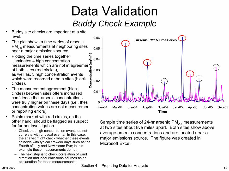
Data ValidationBuddy Check Example
• Buddy site checks are important at a site level.
• The plot shows a time series of arsenic PM2.5 measurements at neighboring sites near a major emissions source.
• Plotting the time series together illuminates 4 high concentration measurements which are not in agreement at both sites (red circles), as well as, 3 high concentration events which were recorded at both sites (black circles).
• The measurement agreement (black circles) between sites offers increased confidence that arsenic concentrations were truly higher on these days (i.e., these concentration values are not measurement or reporting errors).
• Points marked with red circles, on the other hand, should be flagged as suspect for further investigation.
– Check that high concentration events do not correlate with unusual events. In this case, the analyst might check whether these events coincide with typical firework days such as the Fourth of July and New Years Eve; in this example these measurements do not.
– The next step is to check correlation of wind direction and local emissions sources as an explanation for these measurements.
Arsenic PM2.5 Time Series
0
0.01
0.02
0.03
0.04
0.05
0.06
Jan-04 Mar-04 Jun-04 Aug-04 Nov-04 Jan-05 Apr-05 Jun-05 Sep-05Time
Con
cent
ratio
n (u
g/m
^3)
Sample time series of 24-hr arsenic PM2.5 measurements at two sites about five miles apart. Both sites show above average arsenic concentrations and are located near a major emissions source. The figure was created in Microsoft Excel.
June 2009 Section 4 – Preparing Data for Analysis 51
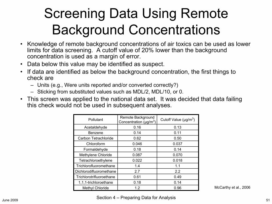
Screening Data Using Remote Background Concentrations
• Knowledge of remote background concentrations of air toxics can be used as lower limits for data screening. A cutoff value of 20% lower than the background concentration is used as a margin of error.
• Data below this value may be identified as suspect.• If data are identified as below the background concentration, the first things to
check are– Units (e.g., Were units reported and/or converted correctly?)– Sticking from substituted values such as MDL/2, MDL/10, or 0.
• This screen was applied to the national data set. It was decided that data failing this check would not be used in subsequent analyses.
Pollutant Remote Background Concentration (µg/m3) Cutoff Value (µg/m3)
Acetaldehyde 0.16 0.13Benzene 0.14 0.11
Carbon Tetrachloride 0.62 0.50Chloroform 0.046 0.037
Formaldehyde 0.18 0.14Methylene Chloride 0.087 0.070Tetrachloroethylene 0.022 0.018
Trichlorofluoromethane 1.4 1.1Dichlorodifluoromethane 2.7 2.2Trichlorotrifluoroethane 0.61 0.49
1,1,1-trichloroethane 0.18 0.14Methyl Chloride 1.2 0.96 McCarthy et al., 2006

June 2009 Section 4 – Preparing Data for Analysis 52
Concentrations (ppb) of carbon tetrachloride (CCl4), dichlorodifluoromethane (CCl2F2), and methyl chloride (CH3Cl) from 2003 and 2004. Northern Hemisphere background concentrations of each species were plotted as a line. Concentration dips well below background concentrations are circled.
0
0.2
0.4
0.6
0.8
1
3/10
/200
3
4/9/
2003
5/9/
2003
6/8/
2003
7/8/
2003
8/7/
2003
9/6/
2003
10/6
/200
3
11/5
/200
3
12/5
/200
3
1/4/
2004
2/3/
2004
3/4/
2004
Date
Con
cent
ratio
n (p
pb)
CCl2F2 CCl4 CH3Cl
CH3Cl Background = 0.6 ppb
CCl2F2 Background = 0.55 ppb
CCl4 Background = 0.09 ppb
Screening Data Using Remote Background Concentrations
Example• This plot shows a time series
plot of concentrations of long-lived species measured at an urban Southwestern site compared to background concentrations measured at remote sites in the Northern Hemisphere.
• Significant spikes and dips in concentrations are circled. Most of the time, concentrations at this monitor were equal to or greater than background concentrations, which might be expected for urban locations.
• Concentrations more than 20% below the background level were identified as suspect for further review.

June 2009 Section 4 – Preparing Data for Analysis 53
• Scatter plot matrices can be used to rapidly and qualitatively examine possible correlations among measured species at a site.
• To interpret a scatter plot matrix, locate the row variable (e.g., methyl ethyl ketone [MEK] in the figure near the top left) and the column variable (e.g., methyl tert-butyl ether [MTBE]) on the bottom. The intersection is the scatter plot of the row variable on the vertical axis against the column variable on the horizontal axis. Each column and row is scaled so that data points fill each frame; scale information is omitted for clarity. The diagonal plots contain histograms of the data for each row variable.
• It is clear that some species correlate well. For example, toluene has a reasonable correlation with ethylbenzene and m- and p-xylene. In contrast, MEK does not correlate with any of the other species; this may indicate that MEK is emitted from different sources. Finally, MTBE shows a bifurcated relationship with toluene, ethylbenzene, and m- and p-xylene. This interesting relationship might be investigated in later validation steps and analysis.
ME
KTO
LE
BE
NZ
MP
XY
LMEK
MTB
ETOL EBENZ MPXYL MTBE
Scatter plot matrix of selected species from an urban site. The species plotted (from top to bottom and left to right) are methyl ethyl ketone (MEK), toluene (TOL), ethylbenzene (EBENZ), m- and p-xylene (MPXYL), and methyl tert-butyl ether (MTBE). The plot was created with SYSTAT11.
Data Validation ExamplesScatter Plots
June 2009 Section 4 – Preparing Data for Analysis 54
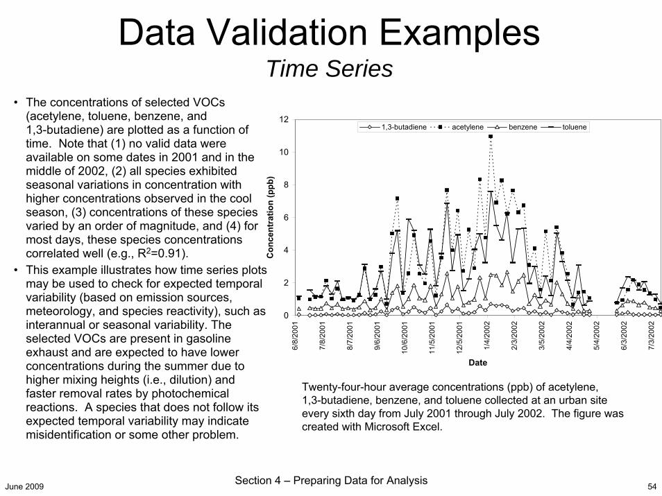
• The concentrations of selected VOCs (acetylene, toluene, benzene, and 1,3-butadiene) are plotted as a function of time. Note that (1) no valid data were available on some dates in 2001 and in the middle of 2002, (2) all species exhibited seasonal variations in concentration with higher concentrations observed in the cool season, (3) concentrations of these species varied by an order of magnitude, and (4) for most days, these species concentrations correlated well (e.g., R2=0.91).
• This example illustrates how time series plots may be used to check for expected temporal variability (based on emission sources, meteorology, and species reactivity), such as interannual or seasonal variability. The selected VOCs are present in gasoline exhaust and are expected to have lower concentrations during the summer due to higher mixing heights (i.e., dilution) and faster removal rates by photochemical reactions. A species that does not follow its expected temporal variability may indicate misidentification or some other problem.
0
2
4
6
8
10
12
6/8/
2001
7/8/
2001
8/7/
2001
9/6/
2001
10/6
/200
1
11/5
/200
1
12/5
/200
1
1/4/
2002
2/3/
2002
3/5/
2002
4/4/
2002
5/4/
2002
6/3/
2002
7/3/
2002
Date
Con
cent
ratio
n (p
pb)
1,3-butadiene acetylene benzene toluene
Twenty-four-hour average concentrations (ppb) of acetylene, 1,3-butadiene, benzene, and toluene collected at an urban site every sixth day from July 2001 through July 2002. The figure was created with Microsoft Excel.
Data Validation ExamplesTime Series
June 2009 Section 4 – Preparing Data for Analysis 55
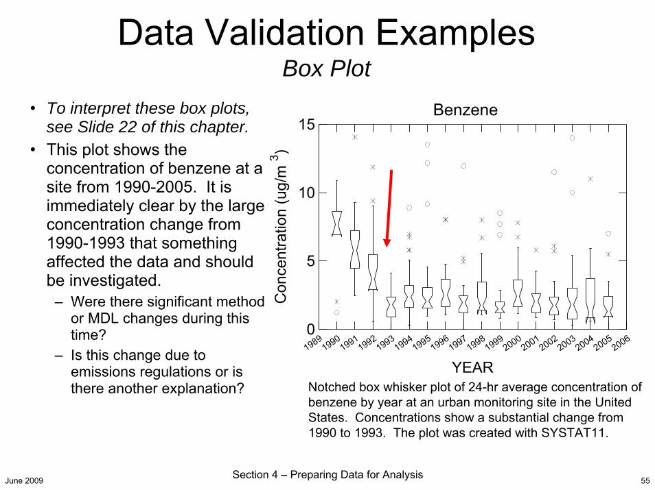
Data Validation ExamplesBox Plot
19891990
19911992
19931994
19951996
19971998
19992000
20012002
20032004
20052006
YEAR
0
5
10
15
Con
cen t
ratio
n (u
g/m
3 )
• To interpret these box plots, see Slide 22 of this chapter.
• This plot shows the concentration of benzene at a site from 1990-2005. It is immediately clear by the large concentration change from 1990-1993 that something affected the data and should be investigated.
– Were there significant method or MDL changes during this time?
– Is this change due to emissions regulations or is there another explanation?
Benzene
Notched box whisker plot of 24-hr average concentration of benzene by year at an urban monitoring site in the United States. Concentrations show a substantial change from 1990 to 1993. The plot was created with SYSTAT11.
June 2009 Section 4 – Preparing Data for Analysis 56
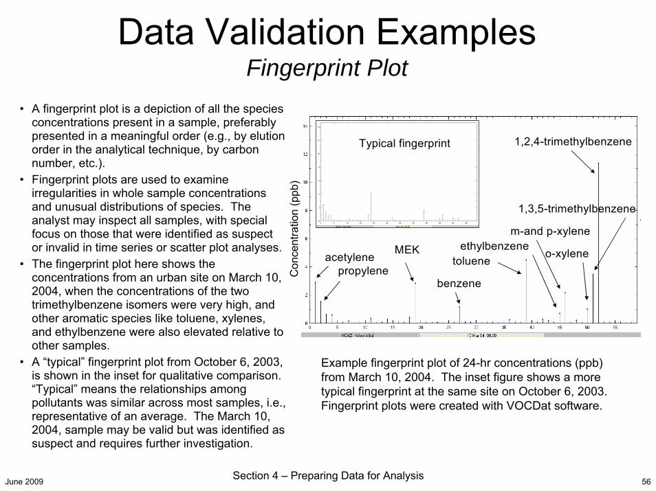
• A fingerprint plot is a depiction of all the species concentrations present in a sample, preferably presented in a meaningful order (e.g., by elution order in the analytical technique, by carbon number, etc.).
• Fingerprint plots are used to examine irregularities in whole sample concentrations and unusual distributions of species. The analyst may inspect all samples, with special focus on those that were identified as suspect or invalid in time series or scatter plot analyses.
• The fingerprint plot here shows the concentrations from an urban site on March 10, 2004, when the concentrations of the two trimethylbenzene isomers were very high, and other aromatic species like toluene, xylenes, and ethylbenzene were also elevated relative to other samples.
• A “typical” fingerprint plot from October 6, 2003, is shown in the inset for qualitative comparison. “Typical” means the relationships among pollutants was similar across most samples, i.e., representative of an average. The March 10, 2004, sample may be valid but was identified as suspect and requires further investigation.
1,2,4-trimethylbenzene
1,3,5-trimethylbenzene
o-xylene
m-and p-xyleneethylbenzene
toluene
benzene
MEKacetylene
propylene
Typical fingerprint
Example fingerprint plot of 24-hr concentrations (ppb) from March 10, 2004. The inset figure shows a more typical fingerprint at the same site on October 6, 2003. Fingerprint plots were created with VOCDat software.
Con
cent
ratio
n (p
pb)
Data Validation ExamplesFingerprint Plot
June 2009 Section 4 – Preparing Data for Analysis 57
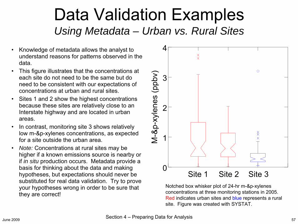
• Knowledge of metadata allows the analyst to understand reasons for patterns observed in the data.
• This figure illustrates that the concentrations at each site do not need to be the same but do need to be consistent with our expectations of concentrations at urban and rural sites.
• Sites 1 and 2 show the highest concentrations because these sites are relatively close to an Interstate highway and are located in urban areas.
• In contrast, monitoring site 3 shows relatively low m-&p-xylenes concentrations, as expected for a site outside the urban area.
• Note: Concentrations at rural sites may be higher if a known emissions source is nearby or if in situ production occurs. Metadata provide a basis for thinking about the data and making hypotheses, but expectations should never be substituted for real data validation. Try to prove your hypotheses wrong in order to be sure that they are correct!
Notched box whisker plot of 24-hr m-&p-xylenes concentrations at three monitoring stations in 2005. Red indicates urban sites and blue represents a rural site. Figure was created with SYSTAT.
Data Validation ExamplesUsing Metadata – Urban vs. Rural Sites
Site 1 Site 2 Site 30
1
2
3
4
M-&
p-xy
lene
s (p
pbv)
June 2009 Section 4 – Preparing Data for Analysis 58
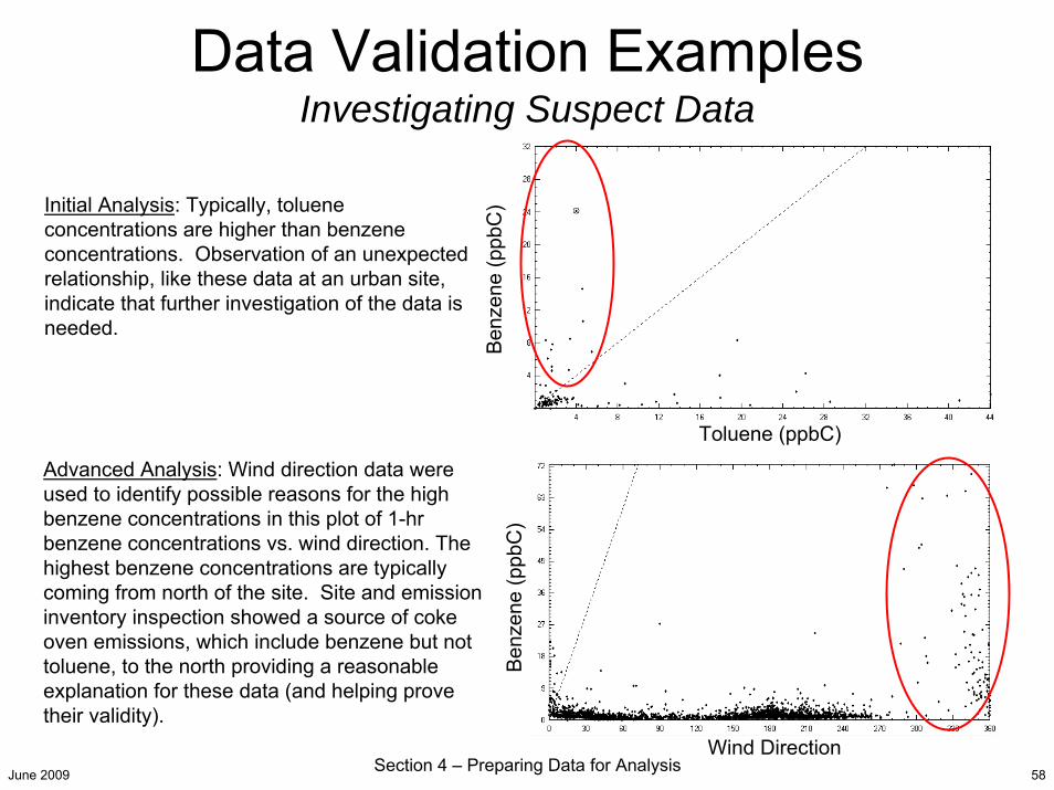
Initial Analysis: Typically, toluene concentrations are higher than benzene concentrations. Observation of an unexpected relationship, like these data at an urban site, indicate that further investigation of the data is needed.
Data Validation ExamplesInvestigating Suspect Data
Advanced Analysis: Wind direction data were used to identify possible reasons for the high benzene concentrations in this plot of 1-hr benzene concentrations vs. wind direction. The highest benzene concentrations are typically coming from north of the site. Site and emission inventory inspection showed a source of coke oven emissions, which include benzene but not toluene, to the north providing a reasonable explanation for these data (and helping prove their validity).
Ben
zene
(ppb
C)
Toluene (ppbC)
Wind Direction
Ben
zene
(ppb
C)
June 2009 Section 4 – Preparing Data for Analysis 59
Data ValidationHandling Suspect Data
• During the process of data validation, the analyst may identify data as suspect but not be able to prove that the data are invalid.
• Analysts may decide to exclude these suspect data from central tendency computations (e.g., annual average) or other analyses.
• These data may warrant additional investigation using case studies (i.e., inspection of individual dates).
June 2009 Section 4 – Preparing Data for Analysis 60
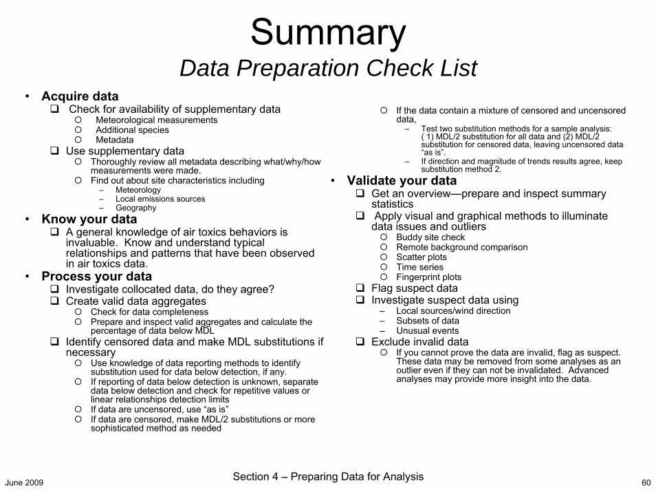
SummaryData Preparation Check List
• Acquire dataCheck for availability of supplementary data
Meteorological measurementsAdditional speciesMetadata
Use supplementary dataThoroughly review all metadata describing what/why/how measurements were made.Find out about site characteristics including
– Meteorology– Local emissions sources– Geography
• Know your dataA general knowledge of air toxics behaviors is invaluable. Know and understand typical relationships and patterns that have been observed in air toxics data.
• Process your dataInvestigate collocated data, do they agree?Create valid data aggregates
Check for data completenessPrepare and inspect valid aggregates and calculate the percentage of data below MDL
Identify censored data and make MDL substitutions if necessary
Use knowledge of data reporting methods to identify substitution used for data below detection, if any.If reporting of data below detection is unknown, separate data below detection and check for repetitive values or linear relationships detection limitsIf data are uncensored, use “as is”If data are censored, make MDL/2 substitutions or more sophisticated method as needed
If the data contain a mixture of censored and uncensored data,
– Test two substitution methods for a sample analysis: ( 1) MDL/2 substitution for all data and (2) MDL/2 substitution for censored data, leaving uncensored data “as is”.
– If direction and magnitude of trends results agree, keep substitution method 2.
• Validate your data Get an overview—prepare and inspect summary statisticsApply visual and graphical methods to illuminate
data issues and outliersBuddy site checkRemote background comparisonScatter plotsTime seriesFingerprint plots
Flag suspect dataInvestigate suspect data using
– Local sources/wind direction– Subsets of data – Unusual events
Exclude invalid dataIf you cannot prove the data are invalid, flag as suspect. These data may be removed from some analyses as an outlier even if they can not be invalidated. Advanced analyses may provide more insight into the data.
June 2009 Section 4 – Preparing Data for Analysis 61
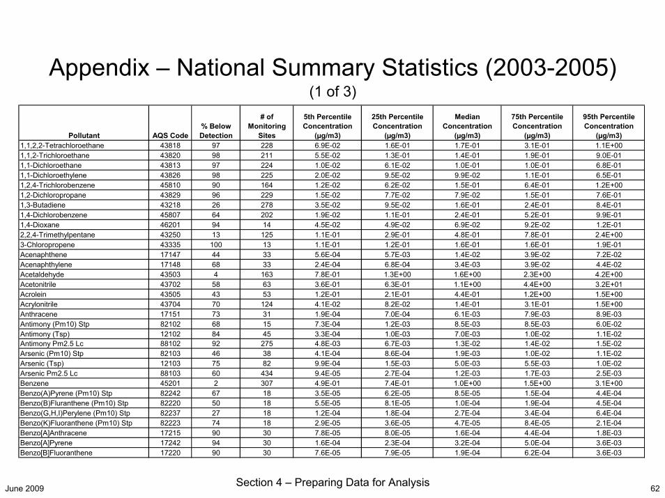
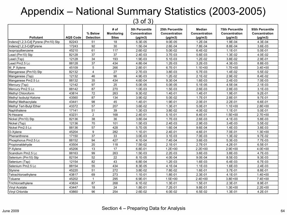
Appendix: National Summary Statistics (2003-2005)
• The appendix contains a table of national summary statistics based upon annual averages from 2003 to 2005.
• These data are useful for comparison of data ranges to “typical”national ranges.
• These data can be used as benchmarks for site-specific comparison; for example, if data are significantly higher than the national 95th percentile, there may be errors in the data.
June 2009 Section 4 – Preparing Data for Analysis 62
Appendix – National Summary Statistics (2003-2005)(1 of 3)
Pollutant AQS Code% Below Detection
# of Monitoring
Sites
5th Percentile Concentration
(µg/m3)
25th Percentile Concentration
(µg/m3)
Median Concentration
(µg/m3)
75th Percentile Concentration
(µg/m3)
95th Percentile Concentration
(µg/m3) 1,1,2,2-Tetrachloroethane 43818 97 228 6.9E-02 1.6E-01 1.7E-01 3.1E-01 1.1E+001,1,2-Trichloroethane 43820 98 211 5.5E-02 1.3E-01 1.4E-01 1.9E-01 9.0E-011,1-Dichloroethane 43813 97 224 1.0E-02 6.1E-02 1.0E-01 1.0E-01 6.8E-011,1-Dichloroethylene 43826 98 225 2.0E-02 9.5E-02 9.9E-02 1.1E-01 6.5E-011,2,4-Trichlorobenzene 45810 90 164 1.2E-02 6.2E-02 1.5E-01 6.4E-01 1.2E+001,2-Dichloropropane 43829 96 229 1.5E-02 7.7E-02 7.9E-02 1.5E-01 7.6E-011,3-Butadiene 43218 26 278 3.5E-02 9.5E-02 1.6E-01 2.4E-01 8.4E-011,4-Dichlorobenzene 45807 64 202 1.9E-02 1.1E-01 2.4E-01 5.2E-01 9.9E-011,4-Dioxane 46201 94 14 4.5E-02 4.9E-02 6.9E-02 9.2E-02 1.2E-012,2,4-Trimethylpentane 43250 13 125 1.1E-01 2.9E-01 4.8E-01 7.8E-01 2.4E+003-Chloropropene 43335 100 13 1.1E-01 1.2E-01 1.6E-01 1.6E-01 1.9E-01Acenaphthene 17147 44 33 5.6E-04 5.7E-03 1.4E-02 3.9E-02 7.2E-02Acenaphthylene 17148 68 33 2.4E-04 6.8E-04 3.4E-03 3.9E-02 4.4E-02Acetaldehyde 43503 4 163 7.8E-01 1.3E+00 1.6E+00 2.3E+00 4.2E+00Acetonitrile 43702 58 63 3.6E-01 6.3E-01 1.1E+00 4.4E+00 3.2E+01Acrolein 43505 43 53 1.2E-01 2.1E-01 4.4E-01 1.2E+00 1.5E+00Acrylonitrile 43704 70 124 4.1E-02 8.2E-02 1.4E-01 3.1E-01 1.5E+00Anthracene 17151 73 31 1.9E-04 7.0E-04 6.1E-03 7.9E-03 8.9E-03Antimony (Pm10) Stp 82102 68 15 7.3E-04 1.2E-03 8.5E-03 8.5E-03 6.0E-02Antimony (Tsp) 12102 84 45 3.3E-04 1.0E-03 7.0E-03 1.0E-02 1.1E-02Antimony Pm2.5 Lc 88102 92 275 4.8E-03 6.7E-03 1.3E-02 1.4E-02 1.5E-02Arsenic (Pm10) Stp 82103 46 38 4.1E-04 8.6E-04 1.9E-03 1.0E-02 1.1E-02Arsenic (Tsp) 12103 75 82 9.9E-04 1.5E-03 5.0E-03 5.5E-03 1.0E-02Arsenic Pm2.5 Lc 88103 60 434 9.4E-05 2.7E-04 1.2E-03 1.7E-03 2.5E-03Benzene 45201 2 307 4.9E-01 7.4E-01 1.0E+00 1.5E+00 3.1E+00Benzo(A)Pyrene (Pm10) Stp 82242 67 18 3.5E-05 6.2E-05 8.5E-05 1.5E-04 4.4E-04Benzo(B)Fluranthene (Pm10) Stp 82220 50 18 5.5E-05 8.1E-05 1.0E-04 1.9E-04 4.5E-04Benzo(G,H,I)Perylene (Pm10) Stp 82237 27 18 1.2E-04 1.8E-04 2.7E-04 3.4E-04 6.4E-04Benzo(K)Fluoranthene (Pm10) Stp 82223 74 18 2.9E-05 3.6E-05 4.7E-05 8.4E-05 2.1E-04Benzo[A]Anthracene 17215 90 30 7.8E-05 8.0E-05 1.6E-04 4.4E-04 1.8E-03Benzo[A]Pyrene 17242 94 30 1.6E-04 2.3E-04 3.2E-04 5.0E-04 3.6E-03Benzo[B]Fluoranthene 17220 90 30 7.6E-05 7.9E-05 1.9E-04 6.2E-04 3.6E-03

June 2009 Section 4 – Preparing Data for Analysis 63
Appendix – National Summary Statistics (2003-2005) (2 of 3)
Benzyl Chloride 45809 95 110 7.4E-03 4.0E-02 1.8E-01 3.7E-01 8.4E-01Beryllium (Pm10) Stp 82105 82 27 2.3E-06 4.1E-06 4.6E-05 3.0E-04 4.6E-04Beryllium (Tsp) 12105 87 62 8.8E-06 2.6E-05 3.0E-05 1.6E-04 2.7E-04Bromoform 43806 100 94 5.2E-02 2.7E-01 5.0E-01 5.2E-01 7.2E-01Bromomethane 43819 92 228 4.4E-02 1.0E-01 1.9E-01 2.1E-01 6.4E-01Cadmium (Pm10) Stp 82110 50 37 1.2E-04 2.4E-04 5.0E-04 9.0E-04 1.2E-03Cadmium (Tsp) 12110 73 105 1.4E-04 3.8E-04 8.0E-04 1.5E-03 2.7E-03Cadmium Pm2.5 Lc 88110 93 263 2.5E-03 2.9E-03 6.4E-03 6.6E-03 6.9E-03Carbon Disulfide 42153 73 75 1.1E-01 1.6E-01 2.6E-01 1.3E+00 3.2E+00Carbon Tetrachloride 43804 42 280 3.3E-01 4.8E-01 5.5E-01 6.3E-01 1.1E+00Chlorine Pm2.5 Lc 88115 67 427 3.4E-04 2.8E-03 1.2E-02 2.9E-02 1.3E-01Chlorobenzene 45801 83 226 1.2E-02 4.4E-02 5.5E-02 1.5E-01 7.6E-01Chloroethane 43812 93 159 1.3E-02 3.9E-02 1.0E-01 1.4E-01 4.4E-01Chloroform 43803 74 273 6.7E-02 1.2E-01 2.4E-01 2.5E-01 8.2E-01Chloromethane 43801 6 245 7.9E-01 1.0E+00 1.2E+00 1.3E+00 1.6E+00Chloroprene 43835 99 114 4.5E-02 4.5E-02 4.5E-02 8.6E-02 5.0E-01Chromium (Pm10) Stp 82112 36 33 4.9E-04 1.0E-03 2.1E-03 2.8E-03 6.2E-03Chromium (Tsp) 12112 67 106 1.3E-03 1.8E-03 2.4E-03 4.8E-03 1.6E-02Chromium Pm2.5 Lc 88112 65 428 3.1E-05 7.0E-05 1.1E-03 2.0E-03 3.2E-03Chromium Vi(Tsp) 12115 55 21 1.3E-05 1.8E-05 2.6E-05 3.8E-05 7.5E-04Chrysene 17208 87 30 1.8E-04 3.1E-04 1.8E-03 3.1E-03 3.2E-03Cobalt (Pm10) Stp 82113 55 23 8.1E-05 1.6E-04 3.0E-04 2.0E-03 4.8E-03Cobalt (Tsp) 12113 66 52 2.0E-04 5.2E-04 9.2E-04 2.0E-03 2.3E-03Cobalt Pm2.5 Lc 88113 96 270 3.2E-04 5.3E-04 8.0E-04 8.2E-04 8.8E-04Dibenz(A-H)Anthracene (Pm10) Stp 82151 91 18 2.5E-05 2.5E-05 2.9E-05 3.6E-05 8.1E-05Dibenzo[A,H]Anthracene 17231 98 30 8.3E-05 1.8E-04 7.8E-04 8.6E-04 3.6E-03Dichloromethane 43802 53 277 1.8E-01 2.4E-01 4.0E-01 8.7E-01 6.1E+00Ethyl Acrylate 43438 100 46 9.6E-02 1.2E-01 1.9E-01 3.3E-01 5.0E-01Ethylbenzene 45203 10 291 1.2E-01 2.5E-01 4.2E-01 6.3E-01 1.0E+00Ethylene Dibromide 43843 98 235 3.8E-02 9.9E-02 1.9E-01 2.2E-01 1.3E+00Ethylene Dichloride 43815 95 253 2.2E-02 1.0E-01 1.0E-01 2.0E-01 6.8E-01Ethylene Oxide 43601 38 16 1.7E-01 1.8E-01 2.1E-01 2.5E-01 4.6E-01Fluoranthene 17201 40 33 3.1E-04 3.2E-04 1.5E-03 3.6E-03 1.8E-02Fluorene 17149 42 33 2.2E-03 4.6E-03 7.8E-03 8.1E-03 3.5E-02Formaldehyde 43502 35 163 1.2E+00 2.0E+00 2.7E+00 3.8E+00 6.7E+00Hexachlorobutadiene 43844 95 153 8.0E-02 1.1E-01 1.7E-01 1.1E+00 1.8E+00Hydrogen Sulfide 42402 91 39 1.0E-03 1.0E-03 1.1E-03 1.5E-03 4.1E-03
Pollutant AQS Code% Below Detection
# of Monitoring
Sites
5th Percentile Concentration
(µg/m3)
25th Percentile Concentration
(µg/m3)
Median Concentration
(µg/m3)
75th Percentile Concentration
(µg/m3)
95th Percentile Concentration
(µg/m3)
June 2009 Section 4 – Preparing Data for Analysis 64
Appendix – National Summary Statistics (2003-2005) (3 of 3)
Indeno[1,2,3-Cd] Pyrene (Pm10) Stp 82243 51 18 5.3E-05 9.0E-05 1.2E-04 1.9E-04 4.3E-04Indeno[1,2,3-Cd]Pyrene 17243 92 30 1.5E-04 2.6E-04 7.8E-04 8.8E-04 3.6E-03Isopropylbenzene 45210 61 117 2.6E-02 5.0E-02 6.4E-02 1.1E-01 5.0E-01Lead (Pm10) Stp 82128 37 37 2.4E-03 3.7E-03 5.6E-03 1.3E-02 4.0E-02Lead (Tsp) 12128 34 193 1.9E-03 5.1E-03 1.2E-02 3.8E-02 2.9E-01Lead Pm2.5 Lc 88128 37 434 4.8E-04 1.2E-03 3.2E-03 4.3E-03 8.8E-03M_P Xylene 45109 5 266 2.8E-01 6.7E-01 1.1E+00 1.7E+00 3.4E+00Manganese (Pm10) Stp 82132 4 27 2.7E-03 3.8E-03 5.7E-03 1.4E-02 5.5E-02Manganese (Tsp) 12132 46 96 4.9E-03 1.2E-02 2.1E-02 2.9E-02 8.4E-02Manganese Pm2.5 Lc 88132 35 434 4.6E-04 9.3E-04 1.6E-03 2.4E-03 7.0E-03Mercury (Tsp) 12142 97 25 5.0E-05 5.0E-05 5.1E-05 4.5E-04 2.1E-03Mercury Pm2.5 Lc 88142 87 270 1.0E-03 1.5E-03 2.6E-03 2.8E-03 3.1E-03Methyl Chloroform 43814 72 263 9.3E-02 1.4E-01 1.4E-01 1.9E-01 9.2E-01Methyl Isobutyl Ketone 43560 87 134 3.9E-02 5.0E-02 1.7E-01 2.8E-01 9.7E-01Methyl Methacrylate 43441 98 45 1.4E-01 1.9E-01 2.0E-01 2.2E-01 6.6E-01Methyl Tert-Butyl Ether 43372 57 207 3.6E-02 1.3E-01 5.0E-01 1.1E+00 2.8E+00Naphthalene 17141 51 39 1.3E-03 3.8E-02 4.0E-02 1.1E-01 5.0E-01N-Hexane 43231 2 168 2.4E-01 5.1E-01 8.4E-01 1.5E+00 2.7E+00Nickel (Pm10) Stp 82136 38 36 3.8E-04 1.7E-03 2.6E-03 4.1E-03 5.8E-03Nickel (Tsp) 12136 70 101 1.5E-03 2.4E-03 2.9E-03 3.4E-03 5.5E-02Nickel Pm2.5 Lc 88136 57 428 5.7E-05 1.6E-04 9.6E-04 1.4E-03 3.8E-03O-Xylene 45204 9 282 1.1E-01 2.4E-01 4.6E-01 7.0E-01 1.3E+00Phenanthrene 17150 37 33 3.0E-03 3.1E-03 7.0E-03 1.3E-02 9.7E-02Phosphorus Pm2.5 Lc 88152 94 427 4.1E-04 7.4E-04 3.6E-03 5.3E-03 7.7E-03Propionaldehyde 43504 20 118 7.5E-02 2.1E-01 2.7E-01 4.2E-01 6.5E-01P-Xylene 45206 13 17 6.8E-01 1.2E+00 2.2E+00 2.9E+00 4.0E+00Scandium Pm2.5 Lc 88163 99 263 1.5E-03 2.2E-03 3.6E-03 3.8E-03 4.7E-03Selenium (Pm10) Stp 82154 52 22 8.1E-05 4.0E-04 9.0E-04 8.5E-03 9.3E-03Selenium (Tsp) 12154 82 43 6.8E-04 1.2E-03 1.6E-03 6.4E-03 6.7E-03Selenium Pm2.5 Lc 88154 55 434 8.3E-05 4.1E-04 1.1E-03 1.6E-03 2.4E-03Styrene 45220 51 272 3.8E-02 7.8E-02 1.6E-01 3.7E-01 8.8E-01Tetrachloroethylene 43817 69 273 1.1E-01 1.8E-01 2.3E-01 4.1E-01 1.4E+00Toluene 45202 1 295 6.9E-01 1.5E+00 2.4E+00 3.8E+00 7.4E+00Trichloroethylene 43824 87 268 6.1E-02 1.3E-01 1.5E-01 2.3E-01 8.9E-01Vinyl Acetate 43447 18 24 1.8E-01 7.2E-01 9.8E-01 1.3E+00 2.2E+00Vinyl Chloride 43860 96 254 2.6E-02 6.0E-02 6.5E-02 1.3E-01 4.2E-01
Pollutant AQS Code% Below Detection
# of Monitoring
Sites
5th Percentile Concentration
(µg/m3)
25th Percentile Concentration
(µg/m3)
Median Concentration
(µg/m3)
75th Percentile Concentration
(µg/m3)
95th Percentile Concentration
(µg/m3)
June 2009 Section 4 – Preparing Data for Analysis 65
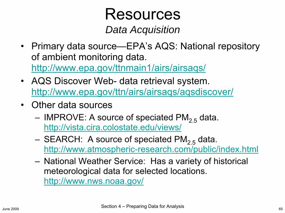
• Primary data source—EPA’s AQS: National repository of ambient monitoring data. http://www.epa.gov/ttnmain1/airs/airsaqs/
• AQS Discover Web- data retrieval system. http://www.epa.gov/ttn/airs/airsaqs/aqsdiscover/
• Other data sources– IMPROVE: A source of speciated PM2.5 data.
http://vista.cira.colostate.edu/views/– SEARCH: A source of speciated PM2.5 data.
http://www.atmospheric-research.com/public/index.html– National Weather Service: Has a variety of historical
meteorological data for selected locations. http://www.nws.noaa.gov/
ResourcesData Acquisition
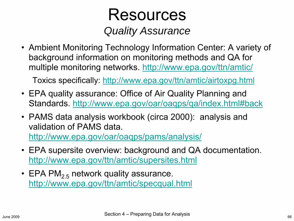
June 2009 Section 4 – Preparing Data for Analysis 66
• Ambient Monitoring Technology Information Center: A variety of background information on monitoring methods and QA for multiple monitoring networks. http://www.epa.gov/ttn/amtic/Toxics specifically: http://www.epa.gov/ttn/amtic/airtoxpg.html
• EPA quality assurance: Office of Air Quality Planning and Standards. http://www.epa.gov/oar/oaqps/qa/index.html#back
• PAMS data analysis workbook (circa 2000): analysis and validation of PAMS data. http://www.epa.gov/oar/oaqps/pams/analysis/
• EPA supersite overview: background and QA documentation. http://www.epa.gov/ttn/amtic/supersites.html
• EPA PM2.5 network quality assurance. http://www.epa.gov/ttn/amtic/specqual.html
ResourcesQuality Assurance
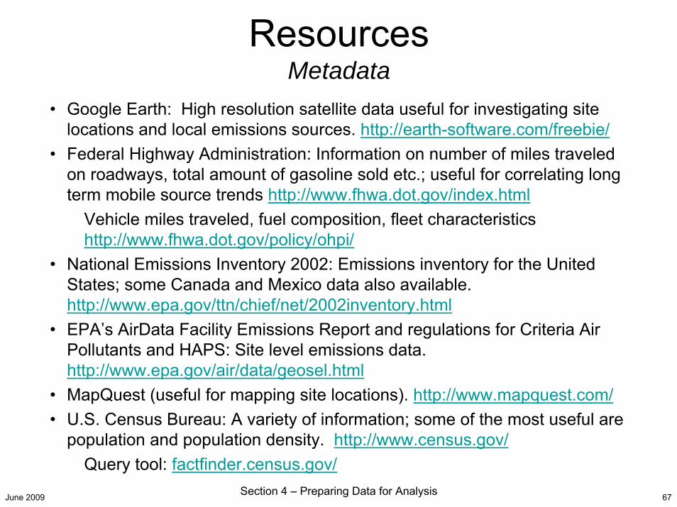
June 2009 Section 4 – Preparing Data for Analysis 67
• Google Earth: High resolution satellite data useful for investigating site locations and local emissions sources. http://earth-software.com/freebie/
• Federal Highway Administration: Information on number of miles traveled on roadways, total amount of gasoline sold etc.; useful for correlating long term mobile source trends http://www.fhwa.dot.gov/index.html
Vehicle miles traveled, fuel composition, fleet characteristics http://www.fhwa.dot.gov/policy/ohpi/
• National Emissions Inventory 2002: Emissions inventory for the United States; some Canada and Mexico data also available. http://www.epa.gov/ttn/chief/net/2002inventory.html
• EPA’s AirData Facility Emissions Report and regulations for Criteria Air Pollutants and HAPS: Site level emissions data. http://www.epa.gov/air/data/geosel.html
• MapQuest (useful for mapping site locations). http://www.mapquest.com/• U.S. Census Bureau: A variety of information; some of the most useful are
population and population density. http://www.census.gov/Query tool: factfinder.census.gov/
ResourcesMetadata
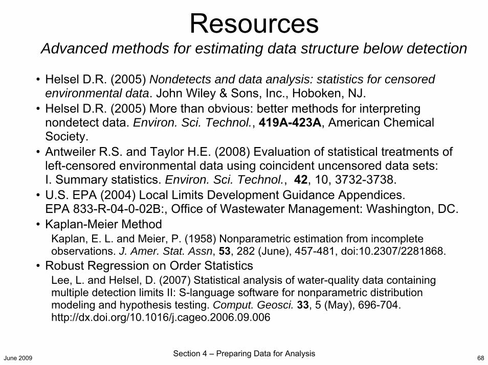
June 2009 Section 4 – Preparing Data for Analysis 68
• Helsel D.R. (2005) Nondetects and data analysis: statistics for censored environmental data. John Wiley & Sons, Inc., Hoboken, NJ.
• Helsel D.R. (2005) More than obvious: better methods for interpreting nondetect data. Environ. Sci. Technol., 419A-423A, American Chemical Society.
• Antweiler R.S. and Taylor H.E. (2008) Evaluation of statistical treatments of left-censored environmental data using coincident uncensored data sets: I. Summary statistics. Environ. Sci. Technol., 42, 10, 3732-3738.
• U.S. EPA (2004) Local Limits Development Guidance Appendices. EPA 833-R-04-0-02B:, Office of Wastewater Management: Washington, DC.
• Kaplan-Meier MethodKaplan, E. L. and Meier, P. (1958) Nonparametric estimation from incomplete observations. J. Amer. Stat. Assn, 53, 282 (June), 457-481, doi:10.2307/2281868.
• Robust Regression on Order StatisticsLee, L. and Helsel, D. (2007) Statistical analysis of water-quality data containing multiple detection limits II: S-language software for nonparametric distribution modeling and hypothesis testing. Comput. Geosci. 33, 5 (May), 696-704. http://dx.doi.org/10.1016/j.cageo.2006.09.006
ResourcesAdvanced methods for estimating data structure below detection
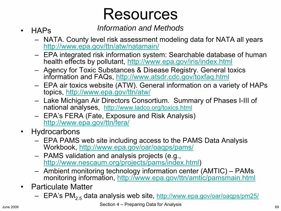
June 2009 Section 4 – Preparing Data for Analysis 69
• HAPs– NATA. County level risk assessment modeling data for NATA all years
http://www.epa.gov/ttn/atw/natamain/– EPA integrated risk information system: Searchable database of human
health effects by pollutant, http://www.epa.gov/iris/index.html– Agency for Toxic Substances & Disease Registry. General toxics
information and FAQs, http://www.atsdr.cdc.gov/toxfaq.html– EPA air toxics website (ATW). General information on a variety of HAPs
topics, http://www.epa.gov/ttn/atw/– Lake Michigan Air Directors Consortium. Summary of Phases I-III of
national analyses, http://www.ladco.org/toxics.html– EPA’s FERA (Fate, Exposure and Risk Analysis)
http://www.epa.gov/ttn/fera/• Hydrocarbons
– EPA PAMS web site including access to the PAMS Data Analysis Workbook, http://www.epa.gov/oar/oaqps/pams/
– PAMS validation and analysis projects (e.g., http://www.nescaum.org/projects/pams/index.html)
– Ambient monitoring technology information center (AMTIC) – PAMs monitoring information, http://www.epa.gov/ttn/amtic/pamsmain.html
• Particulate Matter– EPA’s PM2.5 data analysis web site, http://www.epa.gov/oar/oaqps/pm25/
ResourcesInformation and Methods
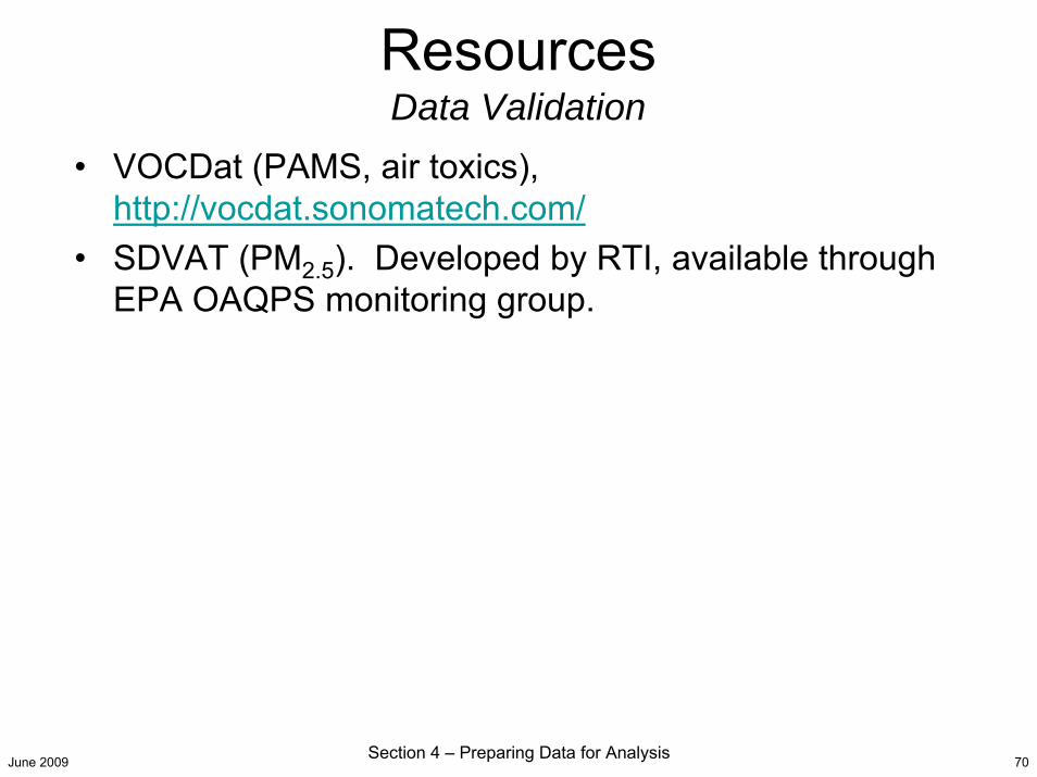
June 2009 Section 4 – Preparing Data for Analysis 70
• VOCDat (PAMS, air toxics), http://vocdat.sonomatech.com/
• SDVAT (PM2.5). Developed by RTI, available through EPA OAQPS monitoring group.
ResourcesData Validation
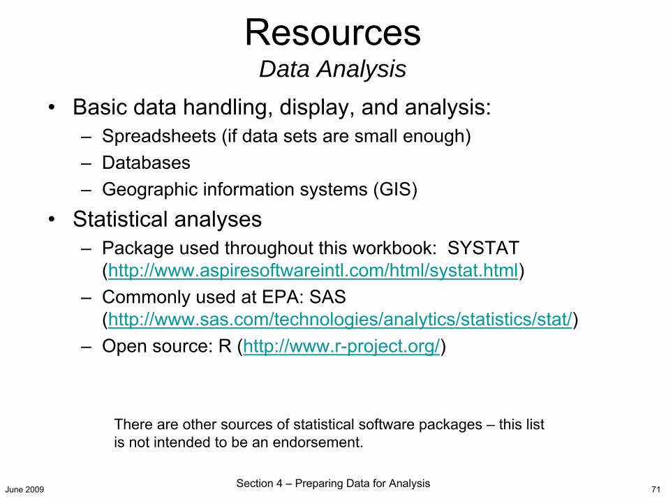
June 2009 Section 4 – Preparing Data for Analysis 71
• Basic data handling, display, and analysis:– Spreadsheets (if data sets are small enough)– Databases– Geographic information systems (GIS)
• Statistical analyses– Package used throughout this workbook: SYSTAT
(http://www.aspiresoftwareintl.com/html/systat.html)– Commonly used at EPA: SAS
(http://www.sas.com/technologies/analytics/statistics/stat/)– Open source: R (http://www.r-project.org/)
ResourcesData Analysis
There are other sources of statistical software packages – this listis not intended to be an endorsement.
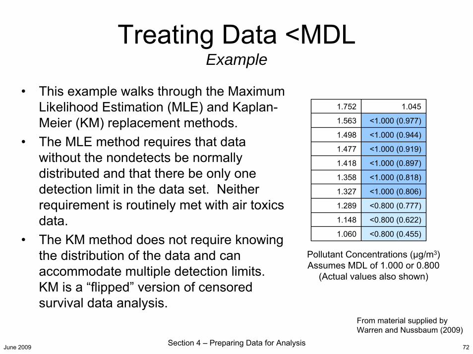
June 2009 Section 4 – Preparing Data for Analysis 72
Treating Data <MDL Example
From material supplied by Warren and Nussbaum (2009)
1.752 1.045
1.563 <1.000 (0.977)
1.498 <1.000 (0.944)
1.477 <1.000 (0.919)
1.418 <1.000 (0.897)
1.358 <1.000 (0.818)
1.327 <1.000 (0.806)
1.289 <0.800 (0.777)
1.148 <0.800 (0.622)
1.060 <0.800 (0.455)
Pollutant Concentrations (µg/m3)Assumes MDL of 1.000 or 0.800
(Actual values also shown)
• This example walks through the Maximum Likelihood Estimation (MLE) and Kaplan-Meier (KM) replacement methods.
• The MLE method requires that data without the nondetects be normally distributed and that there be only one detection limit in the data set. Neither requirement is routinely met with air toxics data.
• The KM method does not require knowing the distribution of the data and can accommodate multiple detection limits. KM is a “flipped” version of censored survival data analysis.
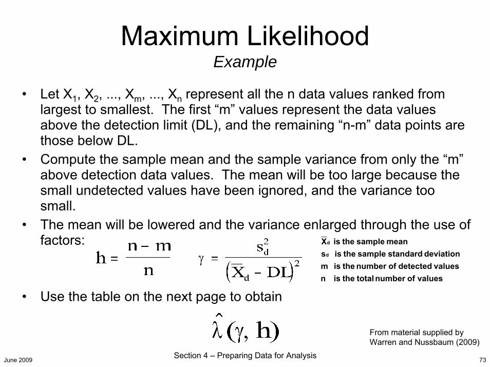
June 2009 Section 4 – Preparing Data for Analysis 73
Maximum LikelihoodExample
From material supplied by Warren and Nussbaum (2009)
• Let X1, X2, ..., Xm, ..., Xn represent all the n data values ranked from largest to smallest. The first “m” values represent the data values above the detection limit (DL), and the remaining “n-m” data points are those below DL.
• Compute the sample mean and the sample variance from only the “m”above detection data values. The mean will be too large because the small undetected values have been ignored, and the variance too small.
• The mean will be lowered and the variance enlarged through the use of factors:
• Use the table on the next page to obtainvalues of number total the is n
values detected of number the is mdeviation standard sample the is s
mean sample the is Xd
d
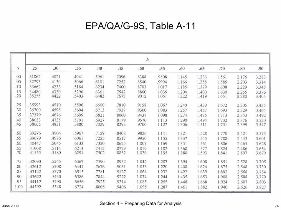
June 2009 Section 4 – Preparing Data for Analysis 74
EPA/QA/G-9S, Table A-11
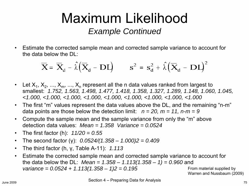
June 2009 Section 4 – Preparing Data for Analysis 75
Maximum LikelihoodExample Continued
• Estimate the corrected sample mean and corrected sample variance to account for the data below the DL:
• Let X1, X2, ..., Xm, ..., Xn represent all the n data values ranked from largest to smallest: 1.752, 1.563, 1.498, 1.477, 1.418, 1.358, 1.327, 1.289, 1.148, 1.060, 1.045, <1.000, <1.000, <1.000, <1.000, <1.000, <1.000, <1.000, <1.000, <1.000
• The first “m” values represent the data values above the DL, and the remaining “n-m”data points are those below the detection limit: n = 20, m = 11, n-m = 9
• Compute the sample mean and the sample variance from only the “m” above detection data values: Mean = 1.358 Variance = 0.0524
• The first factor (h): 11/20 = 0.55• The second factor (γ): 0.0524/(1.358 – 1.000)2 = 0.409 • The third factor (h, γ, Table A-11): 1.113• Estimate the corrected sample mean and corrected sample variance to account for
the data below the DL: Mean = 1.358 – 1.113(1.358 – 1) = 0.960 and variance = 0.0524 + 1.113(1.358 – 1)2 = 0.195 From material supplied by
Warren and Nussbaum (2009)
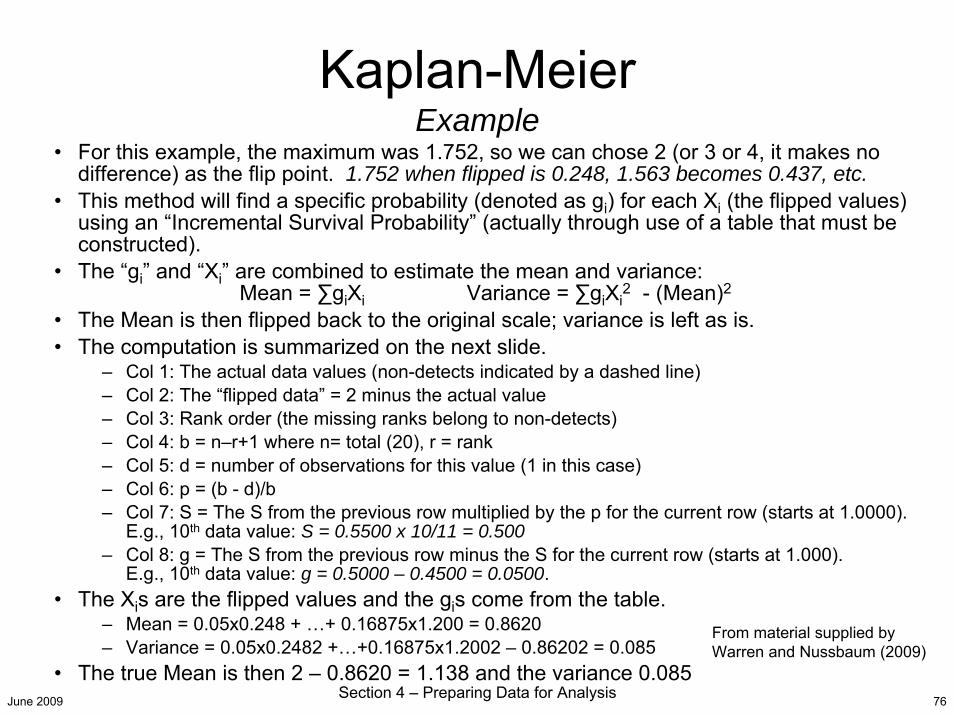
June 2009 Section 4 – Preparing Data for Analysis 76
Kaplan-MeierExample
• For this example, the maximum was 1.752, so we can chose 2 (or 3 or 4, it makes no difference) as the flip point. 1.752 when flipped is 0.248, 1.563 becomes 0.437, etc.
• This method will find a specific probability (denoted as gi) for each Xi (the flipped values) using an “Incremental Survival Probability” (actually through use of a table that must be constructed).
• The “gi” and “Xi” are combined to estimate the mean and variance: Mean = ∑giXi Variance = ∑giXi
2 - (Mean)2
• The Mean is then flipped back to the original scale; variance is left as is.• The computation is summarized on the next slide.
– Col 1: The actual data values (non-detects indicated by a dashed line)– Col 2: The “flipped data” = 2 minus the actual value– Col 3: Rank order (the missing ranks belong to non-detects)– Col 4: b = n–r+1 where n= total (20), r = rank – Col 5: d = number of observations for this value (1 in this case)– Col 6: p = (b - d)/b– Col 7: S = The S from the previous row multiplied by the p for the current row (starts at 1.0000).
E.g., 10th data value: S = 0.5500 x 10/11 = 0.500– Col 8: g = The S from the previous row minus the S for the current row (starts at 1.000).
E.g., 10th data value: g = 0.5000 – 0.4500 = 0.0500.• The Xis are the flipped values and the gis come from the table.
– Mean = 0.05x0.248 + …+ 0.16875x1.200 = 0.8620 – Variance = 0.05x0.2482 +…+0.16875x1.2002 – 0.86202 = 0.085
• The true Mean is then 2 – 0.8620 = 1.138 and the variance 0.085
From material supplied by Warren and Nussbaum (2009)
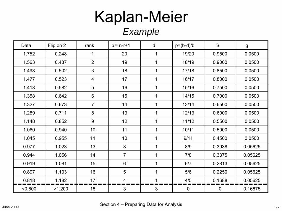
June 2009 Section 4 – Preparing Data for Analysis 77
Kaplan-MeierExample
Data Flip on 2 rank b = n-r+1 d p=(b-d)/b S g
1.752 0.248 1 20 1 19/20 0.9500 0.0500
1.563 0.437 2 19 1 18/19 0.9000 0.0500
1.498 0.502 3 18 1 17/18 0.8500 0.0500
1.477 0.523 4 17 1 16/17 0.8000 0.0500
1.418 0.582 5 16 1 15/16 0.7500 0.0500
1.358 0.642 6 15 1 14/15 0.7000 0.0500
1.327 0.673 7 14 1 13/14 0.6500 0.0500
1.289 0.711 8 13 1 12/13 0.6000 0.0500
1.148 0.852 9 12 1 11/12 0.5500 0.0500
1.060 0.940 10 11 1 10/11 0.5000 0.0500
1.045 0.955 11 10 1 9/11 0.4500 0.0500
0.977 1.023 13 8 1 8/9 0.3938 0.05625
0.944 1.056 14 7 1 7/8 0.3375 0.05625
0.919 1.081 15 6 1 6/7 0.2813 0.05625
0.897 1.103 16 5 1 5/6 0.2250 0.05625
0.818 1.182 17 4 1 4/5 0.1688 0.05625
<0.800 >1.200 18 3 3 0 0 0.16875
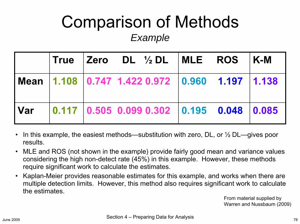
June 2009 Section 4 – Preparing Data for Analysis 78
Comparison of MethodsExample
True Zero DL ½ DL MLE ROS K-M
Mean 1.108 0.747 1.422 0.972 0.960 1.197 1.138
Var 0.117 0.505 0.099 0.302 0.195 0.048 0.085
• In this example, the easiest methods—substitution with zero, DL, or ½ DL—gives poor results.
• MLE and ROS (not shown in the example) provide fairly good mean and variance values considering the high non-detect rate (45%) in this example. However, these methods require significant work to calculate the estimates.
• Kaplan-Meier provides reasonable estimates for this example, and works when there are multiple detection limits. However, this method also requires significant work to calculate the estimates.
From material supplied by Warren and Nussbaum (2009)
June 2009 Section 4 – Preparing Data for Analysis 79
References (1 of 2)
Antweiler R.C. and Taylor H.E. (2008) Evaluation of statistical treatments of left-censored environmental data using coincident uncensored data sets: I. summary statistics. Environ. Sci. Technol. 42 (10), 3732-3738 (10.1021/es071301c).
Bortnick S.M., Coutant B.W., and Biddle B.M. (2003) Estimate background concentrations for the national-scale air toxics assessment. Final technical report prepared for the U.S. Environmental Protection Agency, Research Triangle Park, NC, by Battelle, Columbus, OH, Contract No. 68-D-02-061, Work Assignment 1-03, June.
Helsel D.R. (2005) More than obvious: better methods for interpreting nondetect data. Environ. Sci. Technol., 419A-423A, American Chemical Society.
Helsel D.R. (2005) Nondetects and data analysis: statistics for censored environmental data. John Wiley & Sons, Inc., Hoboken, NJ.
Khalil M.A. and Rasmussen R.A. (1997) The global distribution of atmospheric methyl chloride. Web site of the Climate Monitoring and Diagnostics Laboratory. Available on the Internet at <http://www.cmdl.noaa.gov/publications/annrpt24/khalil.htm>
Kuhlmann et al. (2003) A model for studies of tropospheric ozone and NMHCs: Model evaluation of ozone-related species, J. Geophys. Res. 108(D23) doi:10.1029/2002JD003348.
Main H.H. and Roberts P.T. (2001) PM2.5 data analysis workbook. Draft workbook prepared for the U.S. Environmental Protection Agency, Office of Air Quality Planning and Standards, Research Triangle Park, NC, by Sonoma Technology, Inc., Petaluma, CA, STI-900242-1988-DWB, February.
McCarthy M.C., Hafner H.R., and Montzka S.A. (2006) Background concentrations of 18 air toxics for North America. J. Air and Waste Manag. Assoc. 56, 3-11 (STI-903550-2589). Available on the Internet at http://www.awma.org/journal/ShowAbstract.asp?Year=&PaperID=1509.
Montzka, S.A. et al. (1999) Present and future trends in the atmospheric burden of ozone-depleting halogens. Nature, 398, 690-694.
Parrish D.D., Trainer M., Young V., Goldan P.D., Kuster W.C., Jobson B., T., Fehsenfeld F.C., Lonneman W.A., Zika R.D., Farmer C.T., Riemer D.D., and Rodgers M.O. (1998) Internal consistency tests for evaluation of measurements of anthropogenic hydrocarbons in the troposphere. J. Geophys. Res.-Atmos. 103(D17), 22339-22359.
June 2009 Section 4 – Preparing Data for Analysis 80
References (2 of 2)
Rosenbaum A.S., Axelrad D.A., Woodruff T.J., Wei Y., Ligocki M.P., and Cohen J.P. (1999) National estimates of outdoor air toxics concentrations, J. Air & Waste Manag. Assoc. 49, 1138-1152,.
Singh H.B. et al. (2001) Evidence from the Pacific troposphere for large global sources of oxygenated organic compounds, Nature, 410, 1078-1081.
U.S. Environmental Protection Agency (1980) Validation of air monitoring data. Report prepared by the U.S. Environmental Protection Agency, Research Triangle Park, NC, EPA-600/4-80-030.
U.S. Environmental Protection Agency (1982) Definition and procedure for the determination of the method detection limit - revision 1.11: Federal Register. Pp. 565-567. To be codified at 40 CFR Part 136, Appendix B.
U.S. Environmental Protection Agency (1999) Particulate matter (PM2.5) speciation guidance document. Available at <http://www.epa.gov/ttn/amtic/files/ambient/pm25/spec/specpln3.pdf>.
U.S. Environmental Protection Agency (2004) Local Limits Development Guidance Appendices. EPA 833-R-04-0-02B:, Office of Wastewater Management: Washington, DC.
VIEWS website, http://vista.cira.colostate.edu/views/ Warren, J. and Nussbaum, B. (2009) “Analyzing Datasets Containing Semi-quantitative Values”. Course
material. Office of Environmental Information, EPA Watson J.G., DuBois D.W., DeMandel R., Kaduwela A., Magliano K., McDade C., Mueller P.K., Ranzieri A.,
Roth P.M., and Tanrikulu S. (1998) Aerometric monitoring program plan for the California Regional PM2.5/PM10 Air Quality Study. Draft report prepared for the California Regional PM10/PM2.5 Air Quality Study Technical Committee, California Air Resources Board, Sacramento, CA, by Desert Research Institute, Reno, NV, DRI Document No. 9801.1D5, December.
Weller et al. (2000) Meridional distribution of hydroperoxides and formaldehyde in the MBL of the Atlantic (48 N-35 S) measured during the Albatross campaign. J. Geophys. Res. 105(D11), 14401-14412.
Zhou et al. (1996) Tropospheric formaldehyde concentrations at the Mauna Loa observatory during MLOPEX 2. J. Geophys. Res. 101(D9).