Preference for Boys, Family Size and Educational Attainment in India*

Adriana Kugler1

Santosh Kumar2

May 2015

ABSTRACT

Using data from nationally representative household surveys, we test whether Indian parents make trade-offs between the number of children and investments in education and health of their children. To address the endogeneity due to the joint determination of quantity and quality of children by parents, we instrument family size with the gender of the first child which is plausibly random. Given a strong son-preference in India, parents tend to have more children if the first born is a girl. Our IV results show that children from larger families have lower educational attainment and are less likely to have ever been enrolled and to be currently enrolled in school, even after controlling for parents’ characteristics and birth-order of children. The effects are larger for rural, poorer and low-caste families and for families with less educated mothers. However, we find no evidence of a trade-off for health outcomes.

JEL classification: I15, I2, J13, J18.

Keywords: Quantity-Quality Trade-off, Family size, Education, Health, India

1 McCourt School of Public Policy, Georgetown University, NBER, CEPR, CreAM and IZA. Email: Adriana.Kugler@georgetown.edu. 2 Department of Economics & International Business, Sam Houston State University, Huntsville, TX, 77341-2118, USA. Email: skumar@shsu.edu *We gratefully thank George Akerlof, Richard Akresh, David Albouy, Josh Angrist, Michael Clemens, Shareen Joshi, Dean Karlan, Martin Ravallion, Halsey Rogers, Ganesh Seshan, Gary Solon, Dan Westbrook; seminar participants at the University of Illinois at Urbana-Champaign, at the McCourt School at Georgetown University, at Georgetown University’s Qatar Campus, at the University of Gottingen, at the Inter-American Development Bank and at Sam Houston State University; as well as conference participants at the 9th IZA/World Bank Conference in Employment and Development and the PacDev 2014 Conference for many helpful comments. We also wish to thank Nisha Sinha for excellent research assistance. An earlier version of this paper was circulated as “Testing the Children Quantity-Quality Trade-Off in India”.

1

1. Introduction

High population growth has long been considered a potential deterrent for economic

growth and development because it reduces savings and generates overuse of scarce

resources. By contrast, human capital accumulation is considered one of the main

determinants of income growth. An educated and healthy population is essential for the

production of more sophisticated goods and a key determinant of technical change in the

economy. At the household level, family size and human capital also move in opposite

directions; a larger family has less resources to devote to each child’s education and health.

That is, resource-constrained households may face a quantity-quality trade-off in terms of

their child-rearing decisions (Becker and Lewis 1973).3

In this paper, we test the empirical validity of a children quantity-quality (Q-Q)

trade-off in India. Testing the Q-Q trade-off in the Indian context is interesting because Q-

Q trade-offs are likely to affect additional margins of education and are likely to be stronger

in resource-constrained households in developing countries. In addition, we are able to

exploit the cultural phenomenon of “son preference” in India as a natural experiment to

examine the causal effect of the quantity of children on the investments that parents make

on their children. By contrast, in high income countries, the preference for gender balance

among children is often used as an exogenous source of variation for family size.

Finally, the Indian context is important in its own right if one is trying to understand

low human capital investments in one of the most populous countries in the world. Today,

India is the second most populous country in the world with over 1.2 billion people, and it

3 Becker and Lewis (1973) coined this term and developed the original quantity-quality model.

2

is projected to become the most populous country in the world by 2025. Population growth

in India has been high over the last few decades and continues at 1.4%. Its fertility rate is

still above replacement levels with 2.5 children born per woman. Yet, many children in

India lack access to a good education and health services. According to the 2011 Indian

Census, the literacy rate (age 7 and above) is 73%, meaning that India is home to about 330

million illiterates. The school drop-out rate is alarming as over 80 million children failed to

complete the full cycle of elementary school in 2011 (IHDR, 2011). Furthermore, an

estimated 30% of the world’s malnourished children live in India. The recent HUNGaMA

report (2011) found that 42% of children are underweight and 59 per cent are stunted by

the age of 24 months. The United Nations estimates that 2.1 million Indian children die

before reaching the age of five every year. Thus, against this background, it is important to

quantify the extent to which households make Q-Q trade-offs to understand if family

planning or other policy initiatives that reduce the number of children could also encourage

increased human capital investments by parents.

Empirical testing of the Q-Q trade-off is challenging because fertility decisions and

investments in children are jointly determined and depend on common factors (Browning

1992; Haveman and Wolfe 1995). For example, more educated parents may choose to have

fewer children, but the children of more educated parents are likely to receive more

education themselves. Even if a researcher controls for observable parental characteristics,

parental preferences and other unobservable household characteristics may affect both the

number of children and investments in children. For example, parents who are more

concerned about future opportunities for their children may choose to have fewer children

and also spend more time and educational resources to educate each child. Omitted variable

3

bias of this type will tend to exaggerate the negative relation between family size and human

capital investments.

To address this concern, we employ an Instrumenal Variable strategy (IV) and use

the gender of the first child to instrument family size. A key identification assumption is

that the gender of the first child is a good predictor of the number of children and in the

absence of sex-selective abortion, the gender of the child is random. The preference for

male children in India means that when a household has a first born who is a girl, parents

will continue to have more children until they have a boy. Thus, in a son-biased society,

the first child’s sex should be a good predictor of the probability of having a second child

or of the total number of children in the household. Son preferences are indeed widely

documented in countries such as India, China, and Korea and this preference is deeply

rooted in social, economic and cultural factors (Pande and Astone, 2007).

The other key identification assumption is that the gender of the first-born does not

have an independent impact on the educational performance or health of subsequent

children in the household. There is, indeed, little evidence that households who have a first-

born who is a female are different in other ways from those who have a first-born male.

However, one reason why the gender of the first-born may be related to educational

performance for reasons other than family size is if selective abortions are likely to reduce

the chances of having a first-born who is a girl. Several studies find no evidence of selective

abortions for the first-birth in India, which means that this is unlikely to be a concern in our

study.

We use the District Level Household Survey (DLHS-3) from 2007-08 to examine

the impact on educational outcomes and the National Family Health Survey (NFHS) from

2005-06 to examine the impact of family size on weight and height of young children. Our

4

Ordinary Least Square (OLS) results show negative correlations between family size,

school attendance and years of schooling. While our regressions control for a large number

of children and parental characteristics, there could be unobservable factors related to both

household size and investment in children. We instrument family size by gender of the first

born to address the endogeneity of family size. First-stage results show that having a first-

born who is a female is strongly positively correlated with family size; Anderson-Rubin

and Stock-Wright tests of weak instruments are all rejected.

The IV results show that an extra child in the family reduces schooling by 0.1 years

and reduces the probability of ever attending or being enrolled in school by between 1 and

2 percentage points, respectively. We also find interesting heterogeneous effects. We find

larger effects for rural, poor, and low-caste households as well as for households with

illiterate mothers. The impacts of an extra child in terms of reducing enrollment and

attendance double and the impact of an extra child on years of schooling increase fourfold

for illiterate and poor mothers, suggesting much larger gains from reducing family size in

disadvantaged households. On the other hand, our IV estimates of the impacts of family

size on health outcomes, including, height, weight, height-for-age, weight-for-age, weight-

for-height, malnutrition and stunting show no significant effects. The impact on education

but not on health of children may be due to differences between the public education and

health care systems in India. The public education system is poor and dysfunctional, while

the Indian health care system is designed to provide basic health support even to poor

families; households may also find alternative ways to gain access to health services outside

of the formal health care system.

The rest of the paper proceeds as follows. Section 2 includes a review of the

literature and highlight the contribution of our paper. In Section 3, we present the empirical

5

strategy for the Q-Q trade-off analysis, and Section 4 describes the data. In Sections 5 and

6, we present average and heterogenous effects of family size on education results. The

effects of family size on health are discussed in Section 7, and we conclude in Section 8.

2. Literature Review

Since Becker and Lewis developed the quantity-quality model, a number of studies

have tried to quantify the magnitude of the Q-Q trade off. These studies address the

endogeneity of family size by taking advantage of exogenous variation in policy

experiments (e.g., the one-child policy in China, forced sterilization in India), natural

occurrences of twin births, and sibling sex composition. While the original causal test of

the Q-Q trade-off was conducted using data from India in the 1980s, there has been renewed

attention on this topic in developed and developing countries over the last decade.

Twins have been the most commonly used instrument to study the Q-Q trade-off in

high-income countries, including the U.S., France, Israel, the Netherlands, and Norway.

Black et al. (2005) use twins as an instrument for family size using Norwegian data and

found no evidence that family size affects educational attainment of children, after

controlling for birth order and other potential confounding variables. Similarly, Angrist,

Lavy, and Schlosser (2010) use multiple births and same-sex siblings in families with two

or more children as instruments for family size in Israel. They also fail to find a significant

relation between family size and schooling and employment, but they do find an effect on

women’s early marriage. Haan (2010) concludes that having more children in the family

does not have a significant effect on the educational attainment of the oldest child either in

the U.S. or in the Netherlands. However, a few studies in developed countries did find

evidence of a Q-Q trade-off. Using the Public Use Microdata Sample from the U.S. Census

and gender composition of the first two children as an instrument, Conley and Glauber

6

(2006) demonstrate that children living in larger families are less likely to attend private

school and are more likely to fall behind in school. Similarly, Caceres-Delpiano (2006)

finds that an additional younger sibling in the family reduces the likelihood that older

children attend private school, reduces mother’s participation in the labor market, and

increases the likelihood of their parents’ divorce in the U.S. In contrast, the impact of family

size on measures of child well-being such as highest grade completed and grade retention

is weak and unclear in this study. In a recent working paper, Juhn et al. (2013) instead use

the National Longitudinal Survey of Youth data to examine the impact of family size on

cognitive and non-cognitive abilities during youth as well as long-term outcomes for the

U.S. This study shows that growing up with an additional sibling reduces a child’s

educational attainment by a third of a year; a larger family size decreases labor market

participation and family income, but increases the likelihood of criminal behavior and

teenage pregnancies. A similar study in France also supports Q-Q trade-offs; the school

performance of children from large families was worse than children with smaller families

(Goux and Maurin, 2005). Finally, using marital fecundability-as measured by the time

interval from the marriage to the first birth − as a source of exogenous variation in family

size, Klemp and Weisdorf (2011) document a large and significantly negative effect of

family size on children’s literacy in the UK.

Small or no effects of family size on education and other human capital investments

in developed countries may be caused by the presence of a well-functioning public

education system, which may substitute for private education and may still allow parents

to provide a good education (Li et al., 2008). By contrast, child labor practices and the

absence of good public education may make this trade-off more pronounced in developing

countries, where parental investments in education are a substantial part of a family’s

7

budget.

Rosenzweig and Wolpin (1980) were the first to examine the empirical validity of

Becker-Lewis’s Q-Q trade-off model in a developing country context. They exploited twins

as an exogenous increase in the family size and found a weak negative effect of family size

on educational attainment as well as on consumption durables for non-twin children.

However, the study was based on a small non-representative sample of 1,633 households

that only included 25 households with twins.

In recent years, the Q-Q literature has attained prominence in developing countries

due to bigger families, lower capital investments and failure of family planning policies in

many developing countries. In China, the evidence on Q-Q trade-off is mixed (Li et al.,

2008; Qian, 2009; Rosenzweig and Zhang, 2009). Li et al. (2008) use data from the 1%

sample of the 1990 Chinese Census and rely on twin births as an instrument. They found

that larger family size reduces a child’s education even after controlling for birth order

effects, especially in rural China. In contrast, Qian (2009) uses a sample of households from

China’s Health and Nutritional Survey and relies on the relaxation of the one-child policy

to examine the impact of family size on children’s human capital. She finds a positive effect

of family size on education which she attributes to economies of scale. Rosenzweig and

Zhang (2009), who also rely on twins as an exogenous source of incease in the number of

children, show that an extra child significantly decreases schooling progress, expected

college enrollment, grades in school, and self-assessed health of all children in the family,

thereby concluding that a Q-Q- trade-off does exist in China. However, they argue that the

use of twins as instrument generates upward biases on estimates of the Q-Q trade-off

because of differences in birth weight between twins and non-twins, which changes parental

behavior and overall resource allocation within the household.

8

Studies for other developing countries that mainly rely on the twinning experiment

tend to show either small or no effects. An exception is a study by Jensen (2012) that does

not rely on the twinning experiment; instead infertility was used as an instrument to explore

the causal effects of family size on a child’s nutrition in India and found significant results

only for girls.4 Millimet and Wang (2011) use mixed sex composition to identity the impact

of family size on health outcomes in Indonesia and find evidence of a Q-Q trade-off only

in some families. They find statistically significant results on the Q-Q trade-off only at the

upper and lower tails of the BMI distribution i.e., the 20th and 85th percentile. Using

twinning as an instrument, Ponczek and Souzay (2012) also report negative effects on

educational outcomes in Brazil. Additionally, Glick et al. (2007) use twinning at first birth

and find that unplanned fertility increases the nutritional status and school enrollment of

later-born children in Romania. Using Matlab Health and Socioeconomic Survey from

Bangladesh, Peters et al. (2013) found little evidence of trade-off between child quantity

and health. Dang and Rogers (2013) find that larger family size constrains investments on

schooling in Vietnam.

Sarin (2004) and Lee (2008) are the only other studies, aside from ours, to use

preference for boys as an instrument to study Q-Q trade-off in an under-resourced country.

In a working paper, Sarin (2004) finds no relationship between family size and weight-to-

height ratio using sex of the first-born and multiple births as instruments for family size.5

Lee (2008) is another study that uses preference for boys as an instrument for family size.

4 However, infertility treatments may be used by households, especially by high income households, so this may not be a credible exogenous source of variation.

5 Our paper differs from Sarin (2004) in that we include education in addition to health outcomes. We also use a larger data set, which allows us to include a more complete set of controls (including sibling ordering) and which, covers the time period after the legal ban on fetal sex determination and, thus, provides a more convincing time period to avoid contamination due to sex-selective abortions.

9

However, instead of using direct measures of educational attainment, Lee’s study uses

parents’ monetary investment in education to measure child’s quality. Lee’s IV estimates

show large effects - per-child investment in households with two children and three children

are 74.6 and 57.6% higher, respectively, compared to households with no children.

Our paper adds to the existing literature on Q-Q trade-off in a number of important

ways. First, our study uses a credible and novel instrument, son-preference, in a developing

country context combined with good measures of child quality. This is important because

most studies have relied on the twinning experiment. Second, while many studies have

focused on China and other regions of the developing world, this is the first study to focus

on the impact of family size on educational outcomes in India since the original twinning

study of the 1980s which relied on a very small sample. Not only is India host to 17% of

the world’s population and important in its own right, but lack of good public schools are

likely to affect the extent and severity of the Q-Q trade-off in education. Third, only a

handful of studies have examined the effect of family size on child health; most of the

previous studies have focused on educational attainment/progress. By including health as

an outcome, we contribute to the scant literature on the effect of family size on child health

in a Q-Q framework.

3. Empirical Framework

We estimate the effect of family size on children’s educational and health outcomes

using OLS and 2SLS (instrumental variable) regression analyses. We first estimate the

following OLS model:

𝑌𝑌𝑐𝑐ℎ𝑑𝑑 = 𝛽𝛽0 + 𝛽𝛽1𝐹𝐹𝐹𝐹𝐹𝐹𝐹𝐹𝐹𝐹𝐹𝐹𝐹𝐹𝐹𝐹𝐹𝐹𝑒𝑒ℎ𝑑𝑑 + 𝛽𝛽2𝑋𝑋𝑐𝑐ℎ𝑑𝑑 + 𝜇𝜇𝑑𝑑 + 𝜖𝜖𝑐𝑐ℎ𝑑𝑑 (1)

10

where 𝑌𝑌𝑐𝑐ℎ𝑑𝑑 is the educational or health outcome of child c in household h residing in district

d. The educational outcomes of the child are the probability of ever attending school,

probability of being currently enrolled in school, and years of schooling. We also estimate

similar regressions for several child health measures, including the height-for-age, weight-

for-age, weight-for-height and whether the person is underweight, stunted and wasted. The

variable 𝐹𝐹𝐹𝐹𝐹𝐹𝐹𝐹𝐹𝐹𝐹𝐹𝐹𝐹𝐹𝐹𝐹𝐹𝑒𝑒ℎ𝑑𝑑 is the number of children under 21 years of age in the family; 𝑋𝑋𝑐𝑐ℎ𝑑𝑑

is a vector of covariates, and 𝜖𝜖𝑐𝑐ℎ𝑑𝑑 is an error term. 𝜇𝜇𝑑𝑑 is the district fixed-effects to adjust

for fixed characteristics of the districts. The covariates include the following characteristics

of children and parents: age, gender, caste, birth order and place of residence (rural vs.

urban), and the age and education levels of the parents. The main coefficient of interest is

𝛽𝛽1 which captures the existence of the Q-Q trade-off. A negative value of 𝛽𝛽1 would mean

that a trade-off between the quantity and quality of children does exist in India.

𝛽𝛽1 will provide the causal impact of family size on child quality only if family size

is exogenously determined. However, there are several factors that may render the family

size variable endogenous and non-random. One such factor is the fact that fertility decisions

and decisions about investments in children’s quality are jointly determined. In this case,

the OLS estimate of 𝛽𝛽1 𝐹𝐹𝑖𝑖 Equation 1 is subject to endogeneity bias and is unlikely to

capture the causal effect of family size on child quality. The OLS estimates may be

downwardly or upwardly biased depending on the nature of endogeneity. For example, in

a country like India, wealthier households may have fewer children and also invest more in

their children’s schooling, thus generating an upward bias in the Q-Q trade off. However,

highly committed parents may have more children and also invest more in their children’s

education, thus generating downward biases.

11

In order to capture only exogeneous variation in family size, we rely on an

Instrumental Variable (IV). The challenge with any instrument is to identify a variable that

predicts FamilySize but is uncorrelated with the error term in Equation 1. We use an

indicator for a first-born girl (FBG) as an instrument and estimate the following two-stage

least square model:

𝐹𝐹𝐹𝐹𝐹𝐹𝐹𝐹𝐹𝐹𝐹𝐹𝐹𝐹𝐹𝐹𝐹𝐹𝑒𝑒ℎ𝑑𝑑 = 𝛼𝛼0 + 𝛼𝛼1𝐹𝐹𝐵𝐵𝐵𝐵ℎ𝑑𝑑 + 𝛼𝛼2𝑋𝑋𝑐𝑐ℎ𝑑𝑑 + 𝜇𝜇𝑑𝑑 + 𝑢𝑢𝑐𝑐ℎ𝑑𝑑 (2)

𝑌𝑌𝑐𝑐ℎ𝑑𝑑 = 𝜋𝜋0 + 𝜋𝜋1𝐹𝐹𝐹𝐹𝐹𝐹𝐹𝐹𝐹𝐹𝐹𝐹𝐹𝐹𝐹𝐹𝐹𝐹𝑒𝑒ℎ𝑑𝑑� + 𝜋𝜋2𝑋𝑋𝑐𝑐ℎ𝑑𝑑 + 𝜇𝜇𝑑𝑑 + 𝑣𝑣𝑐𝑐ℎ𝑑𝑑 (3)

where FBG is a dummy variable that equals 1 if the first-born is a female and 0 otherwise

and is used as the instrument for family size. Standard errors are clustered at the district

level.

Equation 2 is the first-stage while Equation 3 is the second-stage regression. The

second stage regresses the outcomes on the predicted value of family size from Equation 2

and other exogenous variables. In addition, we estimate the 2SLS regressions for a number

of sub-groups including: different castes, different levels of household wealth, and different

levels of educational attainment of the mother and for urban and rural sub-samples,

separately.

A key condition for the gender of the first child to be a valid instrument is that

family size be highly correlated with the gender of the first child, i.e., Corr(FBG,

FamilySize)≠ 0. In India, there is a long-standing social and cultural norm of son-

preference for several reasons (Pande and Ashtone, 2007). First, only sons are allowed to

carry forward the family legacy and name. More importantly, since India is a patriarchical

society, sons inherit the family’s patrimony. Second, parents also prefer male children

because sons are supposed to provide financial support and care for their parents in old age.

12

In addition, since men are more likely to enter the labor force and earn higher wages, they

further contribute to a family’s preference for boys. In Indian tradition, daughters are

married out and become part of another family. Because parents have to provide a dowry

when daughters get married, a family will prefer to have boys so they can receive a dowry

when their sons gets married. In this type of patrilineal familial system, the gender of the

first-born is likely to have important implications for family size. In particular, if the first

born is a girl, parents are likely to want to continue having children until a son is born. In

Section 5, we test for this by estimating the first-stage relationship in Equation 2.

The second key underlying assumption behind this identification strategy is that the

sex of the first born is uncorrelated with educational or health outcomes other than through

family size, i.e., Corr(FamilySize, 𝑣𝑣 )=0. Since sex of the first child is determined by nature,

this is considered a random event uncorrelated with educational attainment and health.

However, if parents have any control over births, and they make decisions over births

depending on sex, the sex of the first birth will not be random. Therefore, the presence of

sex-selective abortion may undermine the validity of the instrument because the access to

ultrasound use and abortion services allows parents to choose the sex of their children. Sex-

selective abortions are not as big a concern given that the Pre-natal Diagnostic Technique

Act was passed in India in 1996 making fetal-sex determination illegal. In addition, many

previous studies have shown that parents do not use sex-selective abortions for first-borns

but only for subsequent births in India; these studies find that the sex-ratio at first birth lies

within the biologically range of 1.03-1.07 (Bhalotra and Cochrane, 2010; Jha et al., 2011;

13

Portner, 2015; Rosenblum, 2013a).6 Using the same data as ours, Rosenblum (2013a)

reports lack of sex-selection abortion at the first-parity. About 36% of women report

induced abortions at the second and third-parities. Given that sex-selection abortion became

illegal in India in 1996, zero and positive reporting of induced abortion at first and high-

order, respectively, further provides confidence that sex-selection at first-parity is not

rampant and gender of first-born can be treated as exogenous. Additionally, using the first

two rounds of the National Family and Health Survey, Retherford and Roy (2003) report

little or no evidence of sex selection at the first-birth. Jha et al. (2011) use the National

Family Health Survey and find no significant declines in the sex ratio for first-births or

second-order births if the first-born was a son. Sociological studies also provide evidence

that parents only have a strong preference for sons after the first birth (Patel, 2007). Taken

together, these studies provide evidence that sex of the first-born is indeed exogenous and

random.

To further address the exogeneity of the instrument, we explore whether the

instrument, FBG, is correlated with other observable characteristics of the household to

gauge whether the sex of the first-born can also be assumed to be uncorrelated with

unobservables. Results of the probability models of the sex of the first-born on a vector of

explanatory variables are reported in the next section.

4. Data Description

For educational outcomes, we use data from the Indian District Level Household

Survey (DLHS) collected in 2007-08. The sample is representative at the district level,

6 In the absence of any interventions, the probability of having a son is approximately 0.512, and this probability is independent of genetic factors (Ben-Porath and Welch, 1976; Jacobsen, Mïller and Mouritsen, 1999).

14

which is the lowest tier of administration and policy-making in India. The DLHS covers

601 districts and on average draws a random sample of 1,000-1,500 households from each

district.

DLHS has four parts: a household questionnaire: a questionnaire for ever-married

women (15-49 years); a questionnaire for unmarried women (15-24 years); and a module

covering village and health facilities characteristics. Our study is based on the household

questionnaire, which collected information on assets, number of marriages and deaths in

the household since January 2004, and socio-economic characteristics of all members of

the household. In particular, the survey collects the following information for each

household member: age, gender, schooling attendance, and years of completed schooling.

We identify individuals who are labeled sons/daughters and estimate the family size by

counting the number of sons/daughters in the household, and then merge these data to the

parents’ information.

We restrict the sample in the following ways. First, we restrict the sample to

individuals who are either parents (head of the household and spouse) or who are either

sons/daughters of the head of the household.7 Second, we restrict the sample to households

with at least one child so that we can use the gender of the first child as the instrument.

Third, we restrict the sample to children of school-going-age who are 5 years of age or older

but are under 21. We use 5 as the lower age bound because the household roster only

collects education information of all individuals older than 4. In India, primary school

(grades 1 to 5) begins at age 5 or 6 and ends at age 10 or 11, while high school is usually

completed by age 18. However, completion of either primary or secondary schooling might

7 We drop individuals who are sons- or daughters-in-law, grandchildren, parents, parents-in-law, brothers, sisters, brothers- or sisters-in-law, nieces or nephews, and other relatives.

15

get delayed due to deferred enrollment or grade repetition. We exclude mothers over 35

years of age to minimize the possibility that adult children may have already left the

household. Finally, we exclude households with missing or unreliable information on any

of the variables used in the analysis. This yields a sample of 393,510 children.

The main outcome variables we analyze in this paper are different measures of

educational attainment. The outcome measures include: an indicator of whether the person

ever attended school or not; an indicator of whether the person is currently enrolled in

school or not; and years of schooling. We control for the following covariates in all of the

models: caste, religion, an asset-based standard of living index, mother’s age, father’s age,

mother’s education, and father’s education. For the caste variable, we consider three

groups: scheduled caste and scheduled tribe are combined together to constitute the low

caste category (a group that is socially segregated and disadvantaged), other backward

classes (officially identified as socially and educationally backward) are considered as

middle caste, and the upper caste (comprising Brahmins and other higher castes who are

privileged) are classified as high caste. We consider four major religious groups: Hindus,

Muslims, Sikhs, and Christians. The DLHS data does not contain information on individual

or household incomes. The survey asked a multitude of questions about the ownership of

assets including ownership of a car, television, real state property, and other assets. The

DLHS uses ownership of assets to create a standard of living index with three categories:

low, middle and high.8

8 By combining household amenities, assets and durables, the DLHS data computed a wealth index and divided into quartiles. The principle of factor loading to amenities, assets, and durables derived by factor analysis is used for the computation of the wealth index. Households are categorized from the poorest to the richest groups corresponding to the lowest to the highest quartiles.

16

Table 1 reports the summary statistics of these individual and household variables.

The average age of children in the sample is 10 years and the average years of schooling is

3.08. About 49% of first born children are female. Fathers are older than mothers; the

average age of mothers is 31 years and the average age of fathers is 36. As expected,

mothers have less education than fathers. The average years of schooling for mothers and

fathers are 3.0 and 5.5 years, respectively. The average family size is 3.54. Approximately

82% of children live in rural areas. About 41% of the children are from low caste and 20%

are from high caste. Finally, around 49% of children have the lowest standard of living

index, 39% a middle standard of living, and 12% the highest standard of living.

For health outcomes, we use the National Family Health Survey (NFHS) from 2005-

06. NFHS is India’s primary and only source of data on health and nutrition. Women

between the age of 15-49 were sampled and interviewed to collect anthropometric data for

their children who were under 5 years of age at the time of the survey. The survey collects

anthropometric data for children present in the household at the time of the interview.

Therefore, for analyzing health outcomes, we are constrained to use households where the

oldest child is at most 5 years old at the time of the survey. In particular the survey collects

information on height and weight of the children. Using these anthropometric information,

the NFHS also reports height-for-age z-score, weight-for-age z-score, and weight-for-

height z-score based on World Health Organization guidelines.

We analyze several health outcomes such as weight in kilograms, height in

centimeters, height-for-age z-score (haz), weight-for-age z-score (waz), and weight-for-

height z-score (wfh). In addition, we examine the impact of family size on the probability

of being of underweight (waz < -2 s.d.), on the probability of stunting (haz < -2 s.d.), and

on the probability of the child being wasted (wfh < -2 s.d.). We use the same set of controls

17

as used in the analysis of educational outcomes. The only difference in the econometric

specification is that instead of district fixed-effects, we include state fixed-effects since,

unlike the DLHS, the NFHS does not provide district information.

Our health sample is comprised of 10,090 children with non-missing data on height

and weight. Table 2 provides summary statistics for the health analytical sample. The

average age of children in the sample is 28 months. The average weight-for-age z-score

and height-for-age z-score are -1.63 and -1.47, respectively. Z-scores of minus one and plus

one indicate that a child is one standard deviation below and above the median of the

reference population, respectively. About 39% of sampled children are underweight and

35% of them are stunted. The percentage of wasted children is 15%. A majority of the

children live in rural areas (61%) and the average family size is 2.17.

Table 3 reports the results of linear probability and probit models of the likelihood

that the first-born is a girl on the characteristics as reported in Table 1 to investigate whether

the instrument is likely to be exogeneous. Table 3 shows that most of the explanatory

variables are statistically insignificant except for mother’s age. The older the mother is, the

higher the probability is that the first-born will be a girl. Furthermore, as shown in Table 1,

given that about 49% of first-born are female indicating that the sex-ratio at first-birth is in

the biological range coupled with the results in Table 3, it is reasonable to argue that the

gender of the first-born is likely exogenous.

5. Effects of Family Size on Educational Attainment

The outcome variables in this study include a set of indicators of educational

attainment or educational progress. These include: (a) ever attended school; (b) current

school enrollment; and (c) years of schooling for those who ever attended school. Except

for years of completed schooling, all other variables are binary and are coded as 1 or 0. The

18

main independent variable, household size, is continuous and is measured by the total

number of 0-20 years old children in the family at the time of the survey.

5.1. OLS and IV Impacts of Family Size on Schooling

Table 4 reports the results from the OLS regression. Columns 1-3 report results that

only control for district fixed-effects to account for time-invariant district characteristics.

Columns 4-6 report results with children’s controls, and columns 7-9 report results

controlling also for parents’ characteristics. These results highlight the importance of

controlling for parental characteristics. The magnitude of the estimates of Q-Q coefficient

is bigger when district fixed effects and children’s controls are included but parental

controls are excluded. Adding parental controls in columns 7-9 reduces the coefficient of

family size for all three educational outcomes. The coeffient on ever attended school falls

from -0.022 to -0.018; the coefficient on years of schooling falls from -0.229 to -0.202; and

the coefficient on current enrollment falls from -0.016 to -0.014. These results thus imply

that children in families with one additional child are 1.8 percentage points less likely to

have ever attended school, and the likelihood that they are currently enrolled in school is

1.4 percentage points lower. For years of schooling, the point estimate is -0.2, suggesting

that on average children in families with 5 more siblings will end up with a a year less of

schooling.

Recognizing the limitation of interpreting the OLS estimates in Table 4 as causal,

we then proceed to instrument the main endogenous variable, family size, by an indicator

for the first born being a girl, and then estimate the same relationship using 2SLS. We first

check for the relevance condition in Table 5. From the first-stage regression, it follows that

the instrument is highly significant and has a positive effect on family size. The first row in

19

Table 5 shows that family size increases by 0.22 children when the first-born is a girl and

the effect is significant at 1% level of significance.9

The second row in Table 5 presents results from the estimation of the 2SLS model.

The IV results presented in Table 5 show a negative and significant impact of family size

on children’s quality. The IV estimates for ever being in school and current enrollment are

negative and statistically significant confirming that the detrimental effects of family size

on children’s education comes from both not ever attending school and from dropping out

of school along the way. Columns 1 and 3 show that the probability of ever attending school

and being currently enrolled drop by 1.8 and 1.1 percentage points when an additional

sibling is added to the family. Consequently, years of schooling fall as well. The IV estimate

indicates that an exogenous increase in household size of one extra child decreases the years

of schooling by 0.08 compared to 0.2 when relying on OLS estimates, or 2.6% instead of

6.5%.

Once we account for the endogeneity of family size (using IV), the coefficients are

smaller (or less negative) compared to the ordinary least square estimates. The IV estimates

suggest that OLS coefficients over-estimate the true trade-off and are biased toward finding

effects that are too large suggesting that unobservables which drive parents to have big

families also drive parents to invest too little in their children.

Table 5 also reports the Kleibergen-Paap rk Wald test to detect if the instrument

suffers from a weak-IV problem. The first-stage F-stat and Kleibergen-Paap rk Wald Stat,

both are significant, suggesting that our analysis does not suffer from weak identification.

9 The first stage coefficient is smaller than the twins first-stage of about 0.6 in the Angrist and Evans (1998) study. It is possible that the birth of a girl as the first-born results in a smaller increase in family size due to the fact that Indian families are larger to begin with.

20

We also provide Anderson-Rubin F-test Statistic and Stock-Wright S-statistic in Table 5 to

assess that our second-stage results are robust to weak-instrument inference.

5.2. Potential Threats to Identification

The results in Table 5 show that having a first child who is a girl has a strong positive

effect on family size. Having a first child who is a girl increases the number of children by

a fifth of a child. Moreover, the different tests show that our identification does not suffer

from a weak instrument problem.

Next, we focus on the second key assumption that having a first-child who is a girl

is unlikely to be correlated with other factors associated with educational outcomes. One

potential problem is if the gender of the first child is related to the total children who are

boys in the household. In the U.S., Butcher and Case (1994) find that the sibling sex

composition and, in particular, having more male siblings increases the educational

attainment of girls but not boys in the U.S., probably because girls push themselves more

when they are around male siblings. By contrast, Kaestner (1997) does not find this similar

effect. In the context of a developing country, sibling rivalry or competition for limited

resources may mean that having more male siblings reduces resources for girls.10 To control

for this possibility, Table 6 reports IV estimates controlling for the number of boys in the

household. The results are similar to the IV results without the number of boys but are

somewhat larger. Since the number of boys does itself have a negative impact on some of

the educational outcomes, in the following analysis we continue to control for number of

boys.11

10 Akresh and Edmonds (2011) study find evidence of sibling rivalry in Burkina Faso when households face constraints.

11 However, when we interact an indicator for being a girl with family size, we find no significant difference, suggesting that girls are not particularly hurt by being in larger families. Instead, Barcellos, Carvalho and Lleras-Muney (2014) examine the differential resources invested in boys and girls, controlling for the

21

Another potential reason why the use of gender of the first born could be related to

other factors affecting education is if the likelihood of having a first born who is a girl

increases the likelihood that a mother works in order to be able to pay a dowry for her

daughter’s marriage. We estimate a regression of the likelihood that a mother was employed

in the last 7 days or 12 months on an indicator that the first born was a girl; we find no

effect (Appendix Table 1).

A study by Rosenblum (2013b) shows evidence that son-preferring stopping rules

may mean that the likelihood of survival of a girl is lower.12 Since we only observe

surviving girls who are first born this may mean a positive selection bias in our observed

sample implying we may only be surviving very strong girls with better health. If one

believes that other younger girl siblings following the first born girl are also likely to be

strong, then this would bias the estimates downward, since the strong children in these

households would grow up with more siblings but also would likely do better in school and

in terms of health outcomes. However, a study by Milazzo (2014) instead finds that having

a first born who is a girl increases the likelihood of mortality of the mother after age 30.13

If the death of the mother affects the educational outcomes of children in these households,

this would exaggerate the educational impact atributed to family size. Our analysis is

limited to mothers under 35, and when we further limit our analysis to mothers under 30

the results are similar (Appendix Table 2).

possibility that this might simply be due to girls being in families with more children. 12 Similarly, Hu and Schlosser (2015) find that sex-selective abortion reduces malnutrition for surviving girls. 13 Heath and Xu (2015) examine the impact of the presence of girls (not just the first born) on mother’s

autonomy.

22

6. Heterogeneity in the Quantity-Quality Trade-Off

6.1 . Caste Differences in the Q-Q Trade Off

Given the disadvantaged situation of lower castes in India, one may expect lower

and even middle castes to have less access to good public schools and less access to markets

than higher castes.

We capture the heterogeneity in the Q-Q trade off across different caste categories

by interacting family size with caste. Results from Panel A in Table 7, shows that once the

family size is instrumented,14 the effect of family size on the likelihood of ever attending

school and actual years of schooling is greatest for low caste individuals. For example, an

extra sibling in low and midlle caste households reduces the years of schooling by four

tenths of a year compared to children of high caste households. Similarly, an extra sibling

in low and middle caste households reduces the likelihood of ever attending school by 0.079

and 0.064, respectively, compared to high caste households, although they are not

significantly different from each other. Likewise, growing up with an extra sibling reduces

the likelihood of being currently enrolled by between 0.05 and 0.06 for children in low and

middle caste households compared to those in high caste households. These results thus

suggest that family size has a more negative impact on lower caste families which cannot

overcome educational and liquidity constraints.

6.2. Rural-Urban Differences in the Q-Q Trade Off

Given the lack of good public schools in rural areas in India, we may expect for the

Q-Q trade-off to be greater in rural than in urban areas. Indeed, there are large rural-urban

14 Note that the first stage is similar for different households from different castes, with different wealth levels, with mothers of varying educational levels and for urban and rural households.

23

gaps in educational attainment. For our sample children, the primary school completion rate

is 35% in rural areas while it is 41% in urban areas.

Indeed, the impact of having a larger family size is larger and statistically significant

in rural compared to urban areas, suggesting the quantity-quality trade-off is more

pronounced in rural India. Panel B in Table 7 reports the IV results from models that interact

a rural dummy with the family size variable. The impact of family size on the likelihood

of ever attending school, on years of schooling, and being currently enrolled is greater in

rural than urban households. The coefficients in Table 7 suggest that an extra child reduces

the likelihood of ever attending school or currently attending school by 0.06 and 0.008 and

years of schooling by half a year in rural households compared to urban households. This

finding is similar to Li et al. (2008) who also report that trade-off was more evident in rural

parts of China and was negligible in urban areas.

6.3. Wealth and the Q-Q Trade Off

The degree of the trade-off may also differ by household wealth. Wealthier

households are less likely to be subject to credit constraints when making the choice

between the number of children and the educational opportunities offered to each child. We

classify households by wealth level and estimate interacted IV models with wealth levels

to explore whether the trade-off differs among children from low, median, and high wealth

households. The results in Panel A of Table 8 show the IV results by wealth levels. The

effect of an extra child on the likelihood of going to school, years of schooling, and on the

likelihood of being currently enrolled in school are all greatest for children in poor

households. An extra sibling reduces the likelihood of attending school and being currently

24

enrolled by 0.217 and 0.118 and years of schooling by a year and a month for children in

poor households compared to children in the wealthiest households.

6.4. Does Mother’s Educational Attainment affect the Q-Q Trade Off?

Mothers play a key role in the household by making decisions in regard to

expenditures and by providing a supportive environment for children. Less educated

mothers will generally be worse positioned to provide support for children in their studies

and may not be well informed about possible alternatives to support their children leading

to a bigger Q-Q trade off.

Panel B in Table 8 presents the coefficients of the IV regressions for illiterate

mothers and mothers with less than primary schooling in comparison to the primary

schooled mothers. The IV results show that the detrimental effects of an extra child on

educational attainment are greatest for children of illiterate mothers. The effect of an extra

sibling on years of schooling for the children of illiterate mothers is a little over eight

months compared to those of mothers with at least primary schooling. Even children of

mothers with less than primary education experience a substantially greater trade-off

compared to children of mothers with primary schooling or more. The effect of an extra

child reduces years of schooling by a little over 4 months for those in households of mothers

with less than primary education compared to mothers with a primary education or more.

The trade-off differences are significant for mothers with different education levels.

Similarly, the impacts of an extra sibling on ever having been enrolled or on current

enrollment are greatest for those with either illiterate mothers or mothers with less than a

primary education. An extra sibling reduces the likelihood of ever been enrolled and being

currently enrolled by 0.14 and 0.065, respectively, in households of illiterate mothers

25

compared to mothers with a primary education or more. Children whose mothers have less

than primary education compared to those with primary schooling experience a significant

reduction in the likelihood of ever or being currently enrolled due an extra sibling of 0.076

and 0.056. The Q-Q trade off is significantly stronger for illiterate mothers..

All in all, the Q-Q trade offs are more pronounced among lower caste, rural, and

poorer households, as well as for households headed by less educated mothers, probably

because these households face the greatest credit constraints, attend worse public school

systems, and are less able to compensate for bad schooling by educating their children at

home or by private tutoring.

7. Effect of Family Size on Children’s Health

Child malnourishment is another serious issue that affects investment in human

capital. There is a growing literature on the interaction between early-life health and human

capital accumulation (see Bleakley, 2010, for detail). Bleakley (2010) argues that poor

childhood health might depress the formation of human capital, which in turn can affect

lifetime income either by reducing schooling or limiting labor-market productivity. About

48% of all children in India are malnourished, either moderately or severely underweight

(IIPS, 2010). For many years now, the government of India has implemented several health

programs including the Integrated Child Development Scheme and the National Rural

Health Mission to improve the nutritional status of children. Despite this, malnourishment

levels among Indian children are very high compared to other South Asian countries. It is

plausible that high fertility rates and large families may be contributing to the problem of

malnourishment in India. Given that health is another component of child quality, we test

26

whether there is a trade-off between the number of children and the health of each child in

this section.

We use the National Family Health Survey to examine the trade-off in children’s

health. Table 9 examines the effect of family size on a number of nutrition measures

including height, weight, height-for-age, weight-for-age, weight-for-height, and whether

the person is underweight, wasted, or stunted. Panel A in Table 9 shows the estimates from

OLS while Panel B shows the results from the 2SLS model. The OLS shows that children

of larger families have worse health. Results indicate that an additional child in the

household is associated with a lower average weight of 177 grams and lower average height

of 0.8 cm. Columns 6 and 7 of Table 9 show that children born in larger families are also

more likely to be underweight and stunted, repectively.

Panel B shows the corresponding IV estimates. The IV analysis fails to detect any

significant evidence of Q-Q trade-off in health outcomes. None of the estimates are

statistically significant at conventional levels of significance. This implies that once we

control for the endogeneity of family size, the Q-Q trade-off between family size and health

outcomes disappears. One plausible explanation for these insignificant effects of family

size on nutrition could be that the health system in India, unlike the education system,

provides support to families so that vast trade-offs for children may not be visible.15

8. Conclusions and Discussions

Testing the theoretical trade-off between the quantity and quality of children has

been on the research agenda for a long time, but the empirical evidence supporting the

15 In addition, it is important to point out that while the IV effects are similar or bigger than the OLS effects, the 2SLS results are much less precise. Because we only observe mothers with children younger than 5 years of age, fertility histories of mothers are incomplete in the NFHS sample and the first-stage is not very strong.

27

prediction of the Beckerian model is still limited, especially in developing countries.

Moreover, the empirical evidence has been mixed in general so far. A few studies have

found a negative effect of family size on the quality of children, measured by either

education or health status (Rosenzweig and Wolpin, 1980). In contrast, others reported no

empirical support for the child quantity-quality trade-off (Black et al. 2005; Haan 2010).

A variety of instruments including twinning, sex of first child, sex of first two children,

infertility, and policy experiments were used to address the endogeneity concern.

In this paper, we use data from households in India to test the empirical validity of

the quantity-quality trade-off. A strong preference for sons over daughters in the Indian

society allows us the use of a novel instrumental variable, namely whether the first child is

a girl, to test the Q-Q trade-off. Testing this model has important policy implications as it

is important to know the extent to which a policy formulated to control population improves

the human capital of the country and quality of the labor force.

We find that family size has a significant negative causal impact on educational

outcomes of children. After controlling for potential endogeneity, an additional child in the

family reduces the likelihood of ever having been enrolled and of currently being enrolled

in school as well as years of schooling. The observed trade-off persists after including child

and parent characteristics. We find that the negative relationship between family size and

children’s education is more pronounced among rural households who are severely budget-

constrained. The effect also differs by caste, mother’s education level, and household

wealth. For children belonging to low and middle castes, the trade-off is severe compared

to high-caste children. More educated mothers are also able to mitigate the trade-off

because the trade-off is only evident for illiterate mothers and mothers with less than

primary schooling. Similarly, we observe a wealth-gradient in the trade-off across wealth

28

groups; the trade-off is more pronounced in low-wealth households with an extra child

reducing the years of schooling by as much as a year and a months.

Quantifying the causal estimate of family size on child quality is also important

from a policy perspective. Since the majority of large families in developing countries are

poor, less educated, and resource-constrained, our findings can help us better understand

why poverty persists and how people can be moved out of poverty. Improving access and

uptake of family planning methods and public policies aimed at increasing awareness about

the benefits of having a smaller family may help weaken the severity of the trade-off.

Furthermore, policymakers in developing countries can supplement family planning

policies with more investment in education and health in regions and households for which

the trade-off is severe in order to mitigate the adverse impacts of larger families.

29

References

Akresh, R., and E. V. Edmonds. 2011. “Sibling Rivaly, Residential Rivalry and Constraints on the Availability of Child Labor.” NBER Working Paper 17165.

Angrist, Joshua, and William Evans. 1998. “Children and Their Parents' Labor Supply:

Evidence from Exogenous Variation in Family Size.” American Economic Review 88 (3):45-477.

Angrist, Joshua, Victor Lavy, and Analia Schlosser. 2010. “Multiple Experiments for the

Causal Link between the Quantity and Quality of Children.” Journal of Labor Economics 28:773-824.

Barcellos, Silvia Helena, Leandro S. Carvalho, and Adriana Lleras-Muney. 2014. "Child

Gender and Parental Investments in India: Are Boys and Girls Treated Differently?" American Economic Journal: Applied Economics 6(1):157-89.

Becker, G. S., and H. G. Lewis. 1973. “On the Interaction between the Quantity and Quality

of Children.” Journal of Political Economy 81(2):S279-88. Ben-Porath, Yoram, and Finis Welch. 1976. “Do Sex Preferences Really Matter?”

Quarterly Journal of Economics 90(2):285–307. Bhalotra, Sonia, and Tom Cochrane. 2010. “Where Have All the Young Girls Gone?

Identification of Sex Selection in India.” IZA Discussion Paper 5381. Black, Sandra, Paul Devereux, and Kjell Salvanes. 2005. “The More the Merrier? The

Effect of Family Size and Birth Order on Children’s Education.” Quarterly Journal of Economics 120(2):669-700.

Bleakley, Hoyt. 2010. “Health, Human Capital, and Development.” Annual Reviews of

Economics 2:283-310. Browning, M. 1992. “Children and Household Economic Behavior.” Journal of Economic

Literature 30:1434-75. Butcher, K. F., and Case, A. (1994). “The Effect of Sibling Sex Composition on Women’s

Education and Earnings.” The Quarterly Journal of Economics 109(3):531–563. Caceres-Delpiano, Julio. 2006. "The Impacts of Family Size on Investment in Child

Quality.” Journal of Human Resources XLI (4):738-754. Conley, Dalton, and Rebecca Glauber. 2006. “Parental Educational Investment and

Children’s Academic Risk: Estimates of the Effects of Sibship Size and Birth Order from Exogenous Variation in Fertility.” Journal of Human Resources 41 (4):722-737.

30

Census of India. 2011. Registrar General Office, Government of India. Dang, Hai-Anh and Rogers Halsey. 2013. "The Decision to Invest in Child Quality over

Quantity: Household Size and Household Investment in Education in Vietnam." Policy Research Working Paper 6487, The World Bank.

Glick, P., A. Marini, and D. E. Sahn. 2007. “Estimating the Consequences of Unintended

Fertility for Child Health and Education in Romania: An Analysis using Twins Data.” Oxford Bulletin of Economics & Statistics 69: 667-691.

Goux, Dominique, and Eric Maurin. 2005. “The effect of overcrowded housing on

children’s performance at school.” Journal of Public Economics 89 (5-6):797-819. Haan, Monique De. 2010. “Birth Order, Family Size and Educational Attainment.”

Economics of Education Review 29 (4):576–588. Haveman, R., and B. Wolfe. 1995. “The Determinants of Children's attainment: A Review

of Methods and Findings.” Journal of Economic Literature 33:1829-78. Heath, Rachel and Xu Tan. 2015. “Daughters Improve their Mothers' Autonomy in South

Asia.” Working Paper. Hu, Luojia, and Analia Schlosser. Forthcoming. "Prenatal Sex Selection and Girls Well- Being: Evidence from India.” The Economic Journal. HUNGaMA Report. 2011. "Fighting Hunger and Malnutrition." Naandi Foundation, India. IIPS. 2010. “District Level Household and Facility Survey (DLHS-3), 2007-08.”

International Institute for Population Sciences, Mumbai, India. Indian Human Development Report (IHDR). 2011. "Towards Social Inclusion." Institute of Applied Manpower Research, Planning Commission, Government of India. Jacobsen, R., H. Moller, and A. Mouritsen. 1999. “Natural Variation in the Human Sex

Ratio.” Human Reproduction 14 (12):3120-3125. Jensen, Robert. 2012. “Another Mouth to Feed? The Effects of (In)Fertility on

Malnutrition.” CESifo Economic Studies 58 (2):322-47. Jha, Prabhat, Maya Kesler, Rajesh Kumar, Faujdar Ram , and Usha Ram. 2011. “Trends in

Selective Abortions in India: Analysis of Nationally Representative Birth Histories from 1990 to 2005 and Census Data from 1991 to 2011.” The Lancet 377 (9781): 1921-1928.

31

Juhn, Chinhui, Yona Rubinstein, and Andrew Zuppann. 2013. "The Quantity-Quality Tradeoff and the Formation of Cognitive and Non-cognitive Skills.” University of Houston, Mimeo.

Kaestner, Robert. 1997. “Are Brothers Really Better? Sibling Sex Composition and Educational Achievement Revisited.” Journal of Human Resources 32 (Spring): 250-84. Klemp, Marc, and Jacob Weisdorf. 2011. “The Child Quantity-Quality Trade-Off During

the Industrial Revolution in England.” University of Copenhagen, DP # 11-16. Lee, Jungmin. 2008. “Sibling Size and Investment in Children's Education: An Asian

Instrument.” Journal of Population Economics 21 (4):855-875. Li, Hongbin, Junsen Zhang, and Yi Zhu. 2008. “The Quantity-Quality Trade-Off of

Children in a Developing Country: Identification using Twins.” Demography 45 (1):223-243.

Milazzo, Annamaria. 2014. " Why Are Adult Women Missing? Son Preference and Maternal Survival in India". Policy Research Working Paper 6802, World Bank. Millimet, Daniel L., and Lee Wang. 2011. “Is the Quantity-Quality Trade-Off a Trade-Off

for All, None, or Some?” Economic Development & Cultural Change 60 (1):155-195.

Pande, Rohini P., and Nan Marie Astone. 2007. “Explaining son preference in rural India: the independent role of structural versus individual factors.” Population Research and Policy Review 26 (1):1-29. Patel, Tulsi. 2007. Sex-Selective Abortion in India. New Delhi, India: Sage Publications. Peters, Christina, Daniel I. Rees, and Rey Hernández-Julián. 2013. “The Trade-off between

Family Size and Child Health in Rural Bangladesh.” Eastern Economic Journal 40: 71-95.

Ponczek, Vladimir, and Andre P. Souzay. 2012. “New Evidence of the Causal Effect of

Family Size on Child Quality in a Developing Country.” Journal of Human Resources 47 (1):64-106.

Portner, Claus C. 2015. "Sex-Selective Abortions, Fertility, and Birth Spacing." Policy

Research working paper ; WPS 7189. Washington, DC: World Bank Group. Qian, Nancy. 2009. “Quantity-Quality and the One Child Policy: The Only Child

Disadvantage in School Enrollment in China.” NBER Working Paper No. 14973. Retherford, Robert D., and T. K. Roy. 2003. “Factors Affecting Sex-Selective Abortion in

India and 17 Major States.” NFHS Subject Report 21, IIPS, Mumbai, India.

32

Rosenblum, Dan. 2013a. “Economic Incentives for Sex-Selective Abortion in India.”

Canadian Centre for Health Economics Working Paper No. 2014-13. Rosenblum, Dan. 2013b. “The effect of fertility decisions on excess female mortality in

India." Journal of Population Economics 26(1):147-180. Rosenzweig, M. R., and J. Zhang. 2009. “Do Population Control Policies Induce More

Human Capital Investment? Twins, Birthweight, and China's “One Child” Policy.” Review of Economic Studies 76 (3):1149-1174.

Rosenzweig, M R, and K I Wolpin. 1980. “Testing the Quantity-Quality Fertility Model:

The Use of Twins as a Natural Experiment." Econometrica 48 (1):227-240. Sarin, Ankur. 2004. “Are Children from Smaller Families Healthier?: Examining the

Causal Effects of Family Size on Child Welfare.” University of Chicago, PhD Thesis.

33

Table 1: Descriptive Statistics of the Sample All First Born Girl First Born Boy Children’s Age 9.60 9.41 9.79 (3.45) (3.34) (3.55) First Born Girl 0.49 (0.49) Ever Attended School 0.9 0.89 0.91 (0.30) (0.31) (0.29) Currently Enrolled 0.95 0.95 0.95 (0.21) (0.21) (0.22) Years of Schooling 3.08 2.94 3.22 (2.92) (2.85) (2.98) Mother’s Age 30.94 30.88 31.00 (3.36) (3.34) (3.37) Father’s Age 36.48 36.42 36.54 (4.81) (4.79) (4.82) Mother’s Years of Schooling 2.99 3.05 2.93 (4.06) (4.09) (4.03) Father’s Years of Schooling 5.48 5.56 5.40 (4.74) (4.76) (4.72) Family Size 3.54 3.70 3.40 (1.33) (1.33) (1.31) Rural 0.82 0.81 0.82 (0.39) (0.39) (0.39) Low Caste (SC & ST) 0.41 0.41 0.41 (0.49) (0.49) (0.49) Middle Caste (OBC) 0.39 0.39 0.39 (0.49) (0.49) (0.49) Low Wealth 0.49 0.48 0.49 (0.50) (0.50) (0.50) Medium Wealth 0.39 0.4 0.39 (0.49) (0.49) (0.49) No. of Observations 393,510 193,263 200,247 No. of Districts 601 Notes: Standard deviations are shown in parentheses. All sampled children were 5-20 years old at the time of survey (2007-08). The analytical sample is restricted to 20-35 year old mothers.

34

Notes: Standard deviations appear in the parentheses. Under age-6 sample from NFHS-3 (2005-06). Child is underweight if WAZ < - 2 s.d., child is wasted if HAZ , -2 s.d., child is stunted if WHZ , -2 s.d.

Table 2: Descriptive Statistics of the Health Sample All First Born Girl First Born Boy Children’s Age (months) 28.0 28.31 28.57 (17.01) (17.04) (16.99) First Born Girl 0.51 (0.49) Weight (Grams) 10251.72 10142.56 10363.79 (3123.52) (3061.12) (3182.72) Height (Centimeters) 81.85 81.62 82.10 (13.34) (13.27) (13.42) Weight-for-Age (WAZ) -1.63 -1.64 -1.63 (1.16) (1.17) (1.16) Height-for-Age (HAZ) -1.47 -1.46 -1.48 (1.50) (1.52) (1.48) Weight-for-Height(WHZ) -0.92 -0.92 -0.94 (1.13) (1.12) (1.13) Child is Underweight 0.39 0.39 0.39 (0.49) (0.49) (0.49) Child is Stunted 0.35 0.35 0.35 (0.48) (0.48) (0.48) Child is Wasted 0.15 0.15 0.15 (0.36) (0.36) (0.36) Family Size 2.17 2.20 2.16 (0.42) (0.44) (0.39) Rural 0.61 0.62 0.60 (0.49) (0.49) (0.49) Low caste (SC & ST) 0.33 0.33 0.32 (0.47) (0.47) (0.47) Middle caste (OBC) 0.33 0.33 0.33 (0.47) (0.47) (0.47) Low Wealth 0.29 0.29 0.29 (0.45) (0.45) (0.45) Medium Wealth 0.22 0.22 0.22 (0.41) (0.41) (0.41) Mother’s Age 24.09 24.14 24.04 (3.75) (3.75) (3.74) Father’s Age 29.38 29.46 29.30 (4.79) (4.85) (4.73) Number of Observations 10,090 5,111 4,979 No. of States 29

35

Notes: *, **, and *** represent significance levels of 10, 5, and 1 percent. Robust standard errors, clustered by district, are shown in parentheses. Column 2 reports marginal effects from the probit model.

Table 3: Regression of First Born Girl on Control Variables Dependent Variable: First Born Girl LPM Probit (1) (2) Rural -0.003 -0.008 (0.004) (0.011) Low Wealth -0.002 -0.004 (0.007) (0.017) Medium Wealth -0.004 -0.009 (0.005) (0.013) Hindu 0.006 0.016 (0.00) (0.011) Scheduled Caste/Tribe 0.004 0.009 (0.004) (0.011) Other Backward Caste 0.002 0.006 (0.004) (0.010) Mother’s Years of Schooling 0.002 0.004 (0.001) (0.003) Father’s Years of Schooling -0.0001 -0.0001 (0.001) (0.002) Mother's Age 0.037*** 0.093*** (0.007) (0.017) Father's Age 0.002 0.004 (0.003) (0.008) District Fixed Effects Yes Yes

36

Table 4: OLS Estimates of the Effect of Family Size on Education Ever

Attended School

Years of

Schooling Currently Enrolled

Ever Attended School

Years of

Schooling Currently Enrolled

Ever Attended School

Years of

Schooling Currently Enrolled

(1) (2) (3) (4) (5) (6) (7) (8) (9) Family Size -0.024*** -0.005 -0.019*** -0.022*** -0.229*** -0.016*** -0.018*** -0.202*** -0.014*** (0.001) (0.008) (0.001) (0.001) (0.006) (0.0007) (0.001) (0.006) (0.0006) Children’s Controls No No No Yes Yes Yes Yes Yes Yes Parents’ Controls No No No No No No Yes Yes Yes District Fixed Effects Yes Yes Yes Yes Yes Yes Yes Yes Yes R2 0.07 0.007 0.03 0.13 0.70 0.15 0.14 0.15 No. of Observations 393,510 393,510 345,985 393,510 393,510 345,985 393,510 393,510 345,985 Notes: *, **, and *** represent significance levels of 10, 5, and 1 percent. Robust standard errors, clustered by district, are shown in parentheses. Children’s controls include age, age squared, gender and birth order. Parents’ control includes education levels of father and mother, household religion, household caste, rural, and household socioeconomic status. Family size is total number of 0-20 year old children in the family at the time of the survey.

37

Table 5: IV Estimates of the Effect of Family Size on Children’s Educational Outcomes

Instrument: First Born Girl Ever Attended

School Years of Schooling Currently

Enrolled (1) (2) (3) First Stage 0.219*** 0.219*** 0.228*** (0.007) (0.007) (0.007)

Family Size

-0.018***

-0.080**

-0.011***

(0.007)

1,071.10 4,280.87

10.74 0.001 10.49 0.001

Weak-Identification Tests Kleibergen-Paap Wald rk F-stat Cragg-Donald Wald F-stat Weak-Instrument-Robust –Inference Anderson-Rubin F P-value Stock-Wright S stat P-value

(0.006)

1,071.10 4,280.87

9.43 0.002 9.16 0.003

(0.033)

1,071.10 4,280.87

5.85 0.016 5.71 0.017

Children’s Controls Yes

Yes Yes

Yes Yes Parents’ Controls Yes Yes

Yes District Fixed Effect Yes R2 0.09

393,510 0.68 0.14

345,985 No. of Observations 393,510

Notes: *, **, and *** represent significance levels of 10, 5, and 1 percent. Robust standard error, clustered by district, are shown in parentheses. Children’s controls include age, age square, gender, birth order, religion, caste, SES and rural dummies. Parents’ controls include age, age square, and education levels of father and mother. Family size is total number of 0-20 year old children in the family at the time of the survey.

38

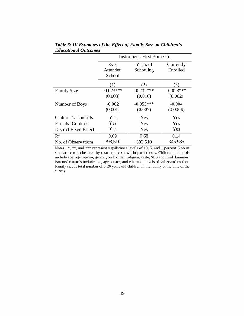
Table 6: IV Estimates of the Effect of Family Size on Children’s Educational Outcomes Instrument: First Born Girl

Ever Attended School

Years of Schooling

Currently Enrolled

(1) (2) (3) Family Size -0.023*** -0.232*** -0.023*** (0.003) (0.016) (0.002)

Number of Boys -0.002 -0.053*** -0.004 (0.001) (0.007) (0.0006)

Children’s Controls Yes Yes Yes

Yes Yes Parents’ Controls Yes Yes

Yes District Fixed Effect Yes R2 0.09

393,510 0.68 0.14

345,985 No. of Observations 393,510 Notes: *, **, and *** represent significance levels of 10, 5, and 1 percent. Robust standard error, clustered by district, are shown in parentheses. Children’s controls include age, age square, gender, birth order, religion, caste, SES and rural dummies. Parents’ controls include age, age square, and education levels of father and mother. Family size is total number of 0-20 years old children in the family at the time of the survey.

39

Table 7: 2SLS Estimates of the Effects of Family Size on Education by Caste and Residence

Ever Attended School

Years of Schooling

Currently Enrolled

(1) (2) (3) Panel A: By Household Caste

Family Size × Low Caste -0.079*** -0.436*** -0.050*** (0.024) (0.131) (0.014)

Family Size × Middle Caste -0.064** -0.440*** -0.061*** (0.022) (0.125) (0.013)

Low Caste 0.252** 1.384** 0.160*** (0.08) (0.444) (0.046)

Middle Caste 0.218** 1.470*** 0.206*** (0.076) (0.428) (0.044)

Family Size 0.041* 0.165 0.032** (0.018) (0.103) (0.011)

No. of Boys -0.002** -0.061*** -0.006*** (0.001) (0.006) (0.001)

Panel B: Rural vs. Urban Family Size × Rural -0.066* -0.537** -0.075***

(0.03) (0.164) (0.018) Family Size 0.038 0.261 0.050***

(0.025) (0.139) (0.015) Rural 0.240* 1.960*** 0.259***

(0.101) (0.56) (0.059) No. of Boys -0.003** -0.065*** -0.007*** (0.001) (0.006) (0.001) Child’s Controls Yes Yes Yes Parents’ Controls Yes Yes Yes District Fixed Effects Yes Yes Yes No. of Observations 393,510 393,597 345,985 Notes: *, **, and *** represent significance levels of 10, 5, and 1 percent. Robust standard errors, by clustered by district, are shown in parentheses. Children’s controls include age, age square, caste, SES and rural dummies. Parents’ controls include age, age square, and education of father and mother, gender, birth order, religion, Family size is total number of 0-20 years old children in the family at the time of the survey. Poor is defined as households in bottom two wealth quartiles. Low caste is scheduled caste (SC) and scheduled tribe (ST) households, while the middle caste is other backward caste (OBC).

40

Table 8: 2SLS Estimates of the Effects of Family Size on Education by Household Wealth and Mother’s Education

Ever Attended School Years of Schooling

Currently Enrolled

(1) (2) (3) Panel A: By Household Wealth

Family Size × Poor -0.217∗∗∗ -1.117∗∗∗ -0.118∗∗∗ (0.058) (0.312) (0.031)

Family Size × Medium -0.155∗∗ -0.905∗∗ -0.116∗∗∗ (0.053) (0.288) (0.029)

Family Size 0.163∗∗ 0.772∗∗ 0.095∗∗∗ (0.053) (0.283) (0.028)

Poor 0.628∗∗∗ 2.890∗∗ 0.314∗∗∗ (0.175) (0.937) (0.094)

Medium 0.436∗∗ 2.407∗∗ 0.318∗∗∗ (0.153) (0.836) (0.085)

No. of Boys -0.001 -0.057∗∗∗ -0.006∗∗∗ (0.001) (0.006) (0.001)

Panel B: by Mother’s Education Family Size × Illiterate -0.140∗∗∗ -0.693∗∗∗ -0.065∗∗∗

(0.025) (0.141) (0.014) Family Size × Less than P i

-0.076∗∗∗ -0.357∗∗ -0.056∗∗∗ (0.020) (0.122) (0.013)

Family Size 0.090∗∗∗ 0.337∗∗ 0.038∗∗∗ (0.020) (0.115) (0.011)

Illiterate 0.428∗∗∗ 2.020∗∗∗ 0.190∗∗∗ (0.079) (0.452) (0.047) Less than Primary 0.233∗∗∗ 1.035∗∗ 0.170∗∗∗

(0.063) (0.376) (0.040) No. of Boys -0.001 -0.051∗∗∗ -0.006∗∗∗ (0.001) (0.006) (0.001) Child’s Controls Yes Yes Yes Parents’ Controls Yes Yes Yes District Fixed Effects Yes Yes Yes No. of Observations 393,510 393,510 345,985 Notes: *, **, and *** represent significance levels of 10, 5, and 1 percent. Robust standard errors, clustered by district, are shown in parentheses. Children’s controls include hge, age square, gender, birth order, religion, caste, SES and rural dummies. Parents’ controls include age, age square, and education of father and mother. Family size is total number of 0-20 years old children in the family at the time of the survey. Poor is defined as households in bottom two wealth quartiles.

41

Table 9: OLS and 2SLS Estimates of the Impact of Family Size on Child’s Health Outcomes

Weight (gram)

Height (cm)

Weight-for-age z-

score

Height-for-age z-

score

Weight-for-height

z-score Underweight (WAZ <-2)

Stunting (HAZ <-2)

Wasting (WHZ <-2)

(1) (2) (3) (4) (5) (6) (7) (8)

Panel A: OLS Results Family Size -177.0***

(46.63) -0.755***

(0.158) -0.114*** (0.0295)

-0.182*** (0.0344)

-0.00350 (0.0270)

0.0371*** (0.0132)

0.0483*** (0.0119)

0.00962 (0.00915)

Panel B: IV Results

First Stage 0.026**

F test of excluded instruments:

F(1, 28) = 5.73 Prob > F = 0.0236

(0.010) Family Size

450.8

7.364

-1.499

-0.858

-0.639

-0.0286

0.00435

0.143

(1,418) (6.658) (1.162) (1.253) (1.252) (0.417) (0.306) (0.323) No. of Obs. 10,107 10,113 10,136 10,136 10,136 10,136 10,136 10,136 Notes: Family size is the number of 0-59 month old children in the family at the time of the survey. All models include child's age, birth order, birth size, gender, religion, caste of the household, rural dummy, mother's education, father's education, mother's age, father's age, socio-economic status of the household and state fixed-effects. Standard errors clustered by state are reported in parentheses. Data source: NFHS

42

Appendix Table 1: Effect of Gender of Child on Mother’s Employment Worked in Last 7

Days Worked in Last 12

Months (1) (2) First Born Girl 0.004 0.0008 (0.003) (0.003)

Children’s Controls Yes Yes Yes

Yes Parents’ Controls Yes

Yes District Fixed Effect R2 0.21

369,586 0.26

No. of Observations 369,586 Notes: *, **, and *** represent significance levels of 10, 5, and 1 percent. Robust standard error, clustered by district, are shown in parentheses. Regression includes the following control varaibles: household size, caste, wealth quartile, religion, literacy status, age, husband’s age, land ownership, and below poverty line status of the household.

43

Appendix Table 2: IV Estimates of the Effect of Family Size on Children’s Educational Outcomes for Young Mothers (Mother’s age < 30)

Instrument: First Born Girl Ever Attended

School Years of Schoolin

g

Currently Enrolled

(1) (2) (3) First Stage 0.219*** 0.188*** 0.195*** (0.007) (0.008) (0.008) Family Size

-0.026***

-0.126**

-0.008** (0.004)

567.50 1558.87

4.08 0.04 4.04 0.04

Weak-Identification Tests Kleibergen-Paap Wald rk F-stat Cragg-Donald Wald F-stat Weak-Instrument-Robust –Inference Anderson-Rubin F P-value Stock-Wright S stat P-value

(0.011)

547.88 1640.85

5.63 0.018 5.53 0.019

(0.038)

547.88 1640.85

10.67 0.001 10.29 0.001

Children’s Controls Yes

Yes Yes

Yes Yes Parents’ Controls Yes Yes

Yes District Fixed-Effect Yes R2 0.10

179,247 0.66 0.06

157,737 No of Observations 179,247 Notes: *, **, and *** represent significance levels of 10, 5, and 1 percent. Robust standard error, clustered by district, are shown in parentheses. Children’s controls include age, age, square, gender, birth order, religion, caste, SES and rural dummies. Parents’ controls include age, age square, and education levels of father and mother. Family size is total number of 0-20 years old children in the family at the time of the survey.

44