prediction of viscous coefficient of venturi meter … · 2018-01-01 · abstract—venturi meters...
TRANSCRIPT

Prediction of Viscous Coefficient of Venturi
Meter under Non ISO Standard Conditions
Karthik Ms1 V Seshadri
2
Department of Mechanical Engineering
Maharaja Institute of Technology, Mysore
Abstract—Venturi meters are commonly used in single and
multiphase flows. The ISO standard (ISO 5167-4) provides
meter discharge coefficients for Venturi meters in turbulent
flows with Reynolds numbers (Re) between 𝟐 × 𝟏𝟎𝟓 to
𝟏 × 𝟏𝟎𝟔, beta value (𝜷) between 0.4 to 0.75 and diameter (D)
between 50mm to 250mm . In viscous fluids, Venturi are
sometimes operated in laminar flows at Reynolds numbers
below the range covered by the standards. The focus of the
study was directed towards very small Reynolds numbers
commonly associated with pipeline transportation of viscous
fluids. However high Reynolds number were also considered.
The Computational Fluid Dynamics (CFD) program STAR
CCM + was used to perform the research. Heavy oil and
water were used separately as the two flowing fluids to obtain
a wide range of Reynolds numbers with high precision.
Multiple models were used with varying characteristics, such
as pipe size and meter geometry, to obtain a better
understanding of the Cd vs. Re relationship.
Keywords - Venturi Meter, Computational Fluid Dynamics
(CFD), Discharge Coefficient, Reynolds Number, Beta Value
I. INTRODUCTION
Among the differential pressure flow meter, Venturi Meter
stands out and dominates in flow measurement field
because of its simple and well understood concept, accurate
and economical compared to other sophisticated flow
meter. Still, study has been made to further understand the
performance of Venturi Tube and its accuracy. Accurate
flow measurement is one of the greatest concerns among
many industries, because uncertainties in product flows can
cost companies considerable profits. Differential pressure
flow meters such as the Venturi, standard concentric orifice
plate, V-cone, and wedge are popular for these applications
at higher Reynolds numbers, because they are relatively
inexpensive and produce reliable results. However, little is
known about their discharge coefficient (Cd) values at low
Reynolds numbers (Miller1) of the Venturi Meter. The
calibrations for these meters are generally performed in a
laboratory using cold water which, at low Reynolds
numbers results in extremely small pressure differentials
that are difficult to measure accurately. Consequently, there
is a need for accurate low Reynolds number flow
measurements for Venturi Meters. In the present work
computational fluid dynamics techniques were utilized to
characterize the behaviour of flow meters from very low to
high Reynolds numbers. In particular, the CFD predictions
of discharge coefficients were validated with results
available in the literature. Results are presented in terms of
predicted discharge coefficients. Reynolds numbers
deserves excessive observation when it comes to analyzing
the capabilities of Venturi Meter. The value of the
Reynolds number for a particular pipe flow can be
decreased by either decreasing the velocity, or increasing
the viscosity. Thus a high viscosity fluid, heavy crude oil
with a viscosity of 0.268 Pa-s is used.
Venturi Meter Discharge Coefficients
Fig-1: Venturi Meter
As Per ISO 5167-4 standard, the mass flow rate in a
Venturi meter (qm) is given by:
qm =Cd
1−β4
πd2
4 2(p1 − p2)ρ
1 .......(1)
Where:
Cd Venturi discharge coefficient
β Venturi beta ratio, d/D
d Venturi throat diameter, mm
D Pipe diameter upstream of the Venturi
convergent section, mm
p1 Static pressure at the upstream pressure tap, Pa
p2 Static pressure at the Venturi throat tap, Pa
ρ1 Fluid density at the upstream tap location,
Kg/mm3
When working with Venturi meters, Reynolds numbers
based on inlet pipe diameter (D) and throat diameter (d) are
frequently used. These are defined as follows:
Re D=
ρvD
μ ....................(2a)
Professor, Department of Mechanical EngineeringMaharaja Institute of Technology,
Mysore
International Journal of Engineering Research & Technology (IJERT)
ISSN: 2278-0181
www.ijert.orgIJERTV4IS051264
(This work is licensed under a Creative Commons Attribution 4.0 International License.)
Vol. 4 Issue 05, May-2015
1338

Re d=
ρvd
μ .....................(2b)
Where µ, ρ and v are the dynamic viscosity, density, and
average velocity, corresponding to inlet pipe diameter (D)
and throat diameter (d) respectively.
Equation (1) is based on the assumptions that include
steady, incompressible, and in-viscid flow (no frictional
pressure losses). Two of the assumptions that are inherent
in the Venturi equation apply when metering viscous
fluids under turbulent flow conditions. These are the
assumptions that make the flow as turbulent, so the
velocity profile is uniform across the cross-section, and
that the frictional pressure losses within the meter can be
neglected.
II. GEOMETRICAL MODEL
Fig-2.1: 2D Model
Fig-2.2: 3D Model
Fig-2.3: 2D Axis-Symmetric Model
The geometries of the Venturi Meter were constructed as
per ISO-5167-4
standards.
Venturi
for 50 to 250mm
diameter pipe at β values 0.4 to 0.75 with 5D upstream and
5D downstream of the Venturi
have been modeled
as
shown in fig-2.1. the convergent section has been taken as
2.7 (D-d) length and 22𝑜 included angle. throat length is
same as the throat diameter d. whereas, the divergent
section has taken as 8𝑜 included angle.
III. NUMERICAL MODEL
CFD modelling is a useful tool to gain an insight into the
physics of the flow and to help understand the test results.
The CFD results were validated by running simulations for
conditions within the range of the ISO standards and
comparing the predicted discharge coefficients with the
ISO standards values. Additional CFD simulations were
conducted to predict discharge coefficient of Venturi meter
at Reynolds numbers below the range covered by the
standards.
The models were created and meshed in STAR CCM+. The
geometries of the Venturi Meter were constructed as per
ISO-5167-4 standards.
Fig-3: Meshed Model, Polyhedral Mesh
Once the geometry was constructed, the geometry is
meshed with various elements like Tria, Quad and
polyhedral elements. After the running the simulations for
multiple meshing schemes, polyhedral cells were the best
fit for the geometry and it is divided approximately into
50,000 cells.
Boundary Conditions:
Fig-3.1: Boundary Conditions
Fig-3.1 shows the boundary conditions applied in STAR
CCM+. The flow inlet on the 5-diameter upstream pipe was
defined as the Velocity Inlet, The flow outlet on the 5-
diameter downstream pipe was defined as a Pressure
Outlet, all solid surfaces are treated as Wall. For 2D axis-
symmetric studies central line has taken as Axis in
simulation.
2D axis-symmetric model has been used for classical
Venturi Meter, the process of grid generation is very
crucial for accuracy, stability and economy of the
prediction of coefficient of discharge. A fine grid leads to
better accuracy and hence it is necessary to generate a
reasonably fine grid in the region of steep velocity
gradients. For efficient discretization the geometry was
divided in to three parts, the upstream and downstream
region and these were meshed with reasonably coarse grid
whereas the central region containing the obstruction
(convergent and divergent zone) and pressure taps was
meshed with very fine grids in order to visualise the effect
of obstruction geometry. The size of grid were kept very
fine in the central region to account for the expected steep
velocity gradients. The grid independence test were carried
out by grid adaptation and comparing the value of Cd
obtained with different grid density, it was found that grid
density after 50000 had very less effect on Cd.
Viscous turbulence model considered for this study was the
realizable k-epsilon model with the standard wall function
enabled. This particular model was used for any of the
International Journal of Engineering Research & Technology (IJERT)
ISSN: 2278-0181
www.ijert.orgIJERTV4IS051264
(This work is licensed under a Creative Commons Attribution 4.0 International License.)
Vol. 4 Issue 05, May-2015
1339

model that had a Reynolds(Re) number greater than 2,000.
The laminar viscosity model was used for any of the
models that had a Re of 2,000 or less. All the constants
associated with this version of STAR CCM+ were left at
their default values.
The study included heavy oil and water as the two different
types of fluids to be examined in order to obtain data for
the entire range of Reynolds numbers. Water was used for
the larger Re(>20,000) while oil was used for the small Re
numbers(<20,000). The primary difference between the
two fluids was that the viscosity of the oil was much
greater than that of water to ensure larger pressure
differences at small Re. The velocity inlet condition only
required the calculated velocity based on Reynolds
numbers. The pressure outlet is set from 1-30 bar normal
downstream pressures. It is important to observe when
studying the results that potential cavitation is not taken
into account using STAR CCM+ therefore high negative
pressures are not a cause for concern.
The pressure velocity coupling used was the Simple
Consistent algorithm. The Under-Relaxation Factors were
set to 0.7 and 0.3 for velocity and pressure. Discretisation factors are vital when regarding the accuracy of the
numerical results. For this study standard pressure was
used, while the Second-Order Upwind method was applied
for momentum, kinetic energy, and the turbulent
dissipation rate.
Residual monitors were used to determine when a solution
had converged to a point where the results had very little
difference between successive iterations. When the k-
epsilon model was applied, there were six different
residuals being monitored which included: continuity, x, y,
and z velocities, k, and epsilon. The study aimed to ensure
the utmost iterative accuracy by requiring all of the
residuals to converge to 1e-05, before the model runs were
complete.
IV. RESULTS AND DISCUSSION
There are many pipelines where flows need to be
accurately measured. Meters having a high level of
accuracy and relatively low cost are a couple of the most
important parameters when deciding on the purchase of a
flow meter. Most differential pressure flow meters meet
both of these requirements. Many of the most common
flow meters have a specified range where the discharge
coefficient may be considered constant and where the
lower end is usually the minimum recommended Re
number that should be used with the specified meter. With
the additional knowledge of this study it will enable the
user to better estimate the flow through a pipeline over a
wider range of Reynolds numbers. The research completed
in this study on discharge coefficients focused on Venturi
Meter with varying beta ratios and diameters.
It was seen that the best way to present the data for
interpretation is by using semi-log graphs for plotting
discharge coefficient vs. Reynolds number. Each of the
data points on the graphs was computed separately based
on the performance from a Reynolds number. The
velocities that were needed to obtain different Reynolds number values were the primary variable put into the
numerical model when computing each discharge
coefficients. Heavy Oil was used for flows where Re <
20,000 while water was used for higher turbulent flow test
runs.
Venturi flow meter models were created to determine their
discharge coefficient for a wide range of Reynolds
numbers. The different β values used for the models were
0.661and 0.5 with diameters of 230mm and154.1mm to
observe if there was any significant difference in results
based on pipe diameter.
The Venturi meter was modelled using different geometries
to determine if there was significant effect on the resultant
Cd over the Re range. It was found that the data sets
followed very similar trends despite having different
geometries.
Fig-4: comparison of present study vs. miller physical study.
Re Cd
Present Study Miller,2009
100000 0.985 0.98
50000 0.98 0.98
10000 0.96 0.94
5000 0.945 0.92
1000 0.912 0.87
500 0.848 0.8
100 0.661 0.59
10 0.336
1 0.112
Table-1: comparison of present study vs. miller physical study.
As illustrated in the fig-4 the simulation presented in the
present work were in close agreement with the Miller1
experimental values for the Reynolds number ranging from
100 to 1,00,000. Miller1, used a multiphase flow of heavy
oil and water through the Venturi meters tested, which may
be the reason that the Cd values decrease more rapidly than
the present study. the multiphase flow was not completely
00.10.20.30.40.50.60.70.80.91
1 10 100 1000 10000 100000
present studyMiller,2009
Re
Cd
Plot of Cd vs. Re
International Journal of Engineering Research & Technology (IJERT)
ISSN: 2278-0181
www.ijert.orgIJERTV4IS051264
(This work is licensed under a Creative Commons Attribution 4.0 International License.)
Vol. 4 Issue 05, May-2015
1340
mixed, some of the oil may settle at the entrance of the
Ventrui Meter.
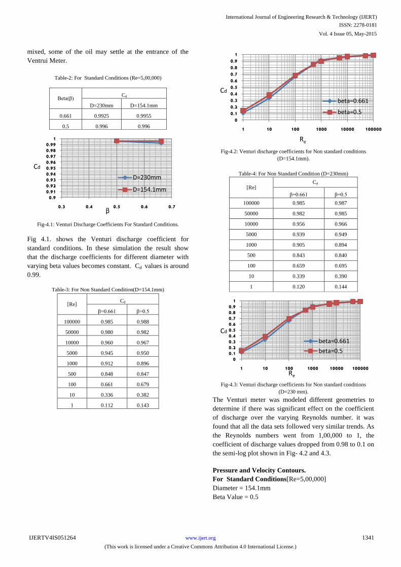
Table-2: For Standard Conditions (Re=5,00,000)
Beta(β) Cd
D=230mm D=154.1mm
0.661 0.9925 0.9955
0.5 0.996 0.996
Fig-4.1: Venturi Discharge Coefficients For Standard Conditions.
Fig 4.1. shows the Venturi discharge coefficient for
standard conditions. In these simulation the result show
that the discharge coefficients for different diameter with
varying beta values becomes constant. Cd values is around
0.99.
Table-3: For Non Standard Condition(D=154.1mm)
[Re] Cd
β=0.661 β=0.5
100000 0.985 0.988
50000 0.980 0.982
10000 0.960 0.967
5000 0.945 0.950
1000 0.912 0.896
500 0.848 0.847
100 0.661 0.679
10 0.336 0.382
1 0.112 0.143
Fig-4.2: Venturi discharge coefficients for Non standard conditions
(D=154.1mm).
Table-4: For Non Standard Condition (D=230mm)
[Re] Cd
β=0.661 β=0.5
100000 0.985 0.987
50000 0.982 0.985
10000 0.956 0.966
5000 0.939 0.949
1000 0.905 0.894
500 0.843 0.840
100 0.659 0.695
10 0.339 0.390
1 0.120 0.144
Fig-4.3: Venturi discharge coefficients for Non standard conditions
(D=230 mm).
The Venturi meter was modeled different geometries to
determine if there was significant effect on the coefficient
of discharge over the varying Reynolds number. it was
found that all the data sets followed very similar trends. As
the Reynolds numbers went from 1,00,000 to 1, the
coefficient of discharge values dropped from 0.98 to 0.1 on
the semi-log plot shown in Fig- 4.2 and 4.3.
Pressure and Velocity Contours.
For Standard Conditions[Re=5,00,000]
Diameter = 154.1mm
Beta Value = 0.5
0.90.910.920.930.940.950.960.970.980.99
1
0.3 0.4 0.5 0.6 0.7
D=230mm
D=154.1mm
β
00.10.20.30.40.50.60.70.80.91
1 10 100 1000 10000 100000
beta=0.661
beta=0.5
Cd
Re
00.10.20.30.40.50.60.70.80.91
1 10 100 1000 10000 100000
beta=0.661
beta=0.5
Cd
Re
Cd
International Journal of Engineering Research & Technology (IJERT)
ISSN: 2278-0181
www.ijert.orgIJERTV4IS051264
(This work is licensed under a Creative Commons Attribution 4.0 International License.)
Vol. 4 Issue 05, May-2015
1341
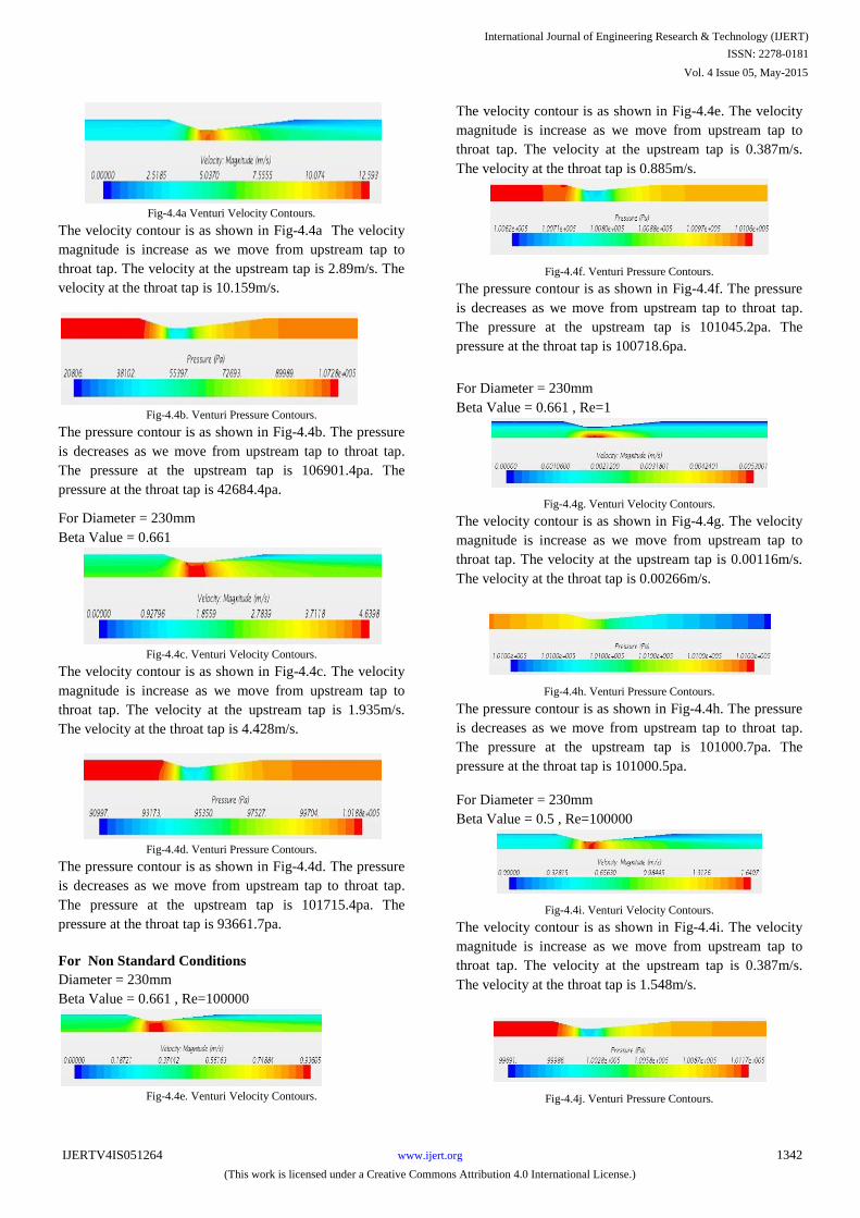
Fig-4.4a Venturi Velocity Contours.
The velocity contour is as shown in Fig-4.4a The velocity
magnitude is increase as we move from upstream tap to
throat tap. The velocity at the upstream tap is 2.89m/s. The
velocity at the throat tap is 10.159m/s.
Fig-4.4b. Venturi Pressure Contours.
The pressure contour is as shown in Fig-4.4b. The pressure
is decreases as we move from upstream tap to throat tap.
The pressure at the upstream tap is 106901.4pa. The
pressure at the throat tap is 42684.4pa.
For Diameter = 230mm
Beta Value = 0.661
Fig-4.4c. Venturi Velocity Contours.
The velocity contour is as shown in Fig-4.4c. The velocity
magnitude is increase as we move from upstream tap to
throat tap. The velocity at the upstream tap is 1.935m/s.
The velocity at the throat tap is 4.428m/s.
Fig-4.4d. Venturi Pressure Contours.
The pressure contour is as shown in Fig-4.4d. The pressure
is decreases as we move from upstream tap to throat tap.
The pressure at the upstream tap is 101715.4pa. The
pressure at the throat tap is 93661.7pa.
For Non Standard Conditions
Diameter = 230mm
Beta Value = 0.661 , Re=100000
Fig-4.4e. Venturi Velocity Contours.
The velocity contour is as shown in Fig-4.4e. The velocity
magnitude is increase as we move from upstream tap to
throat tap. The velocity at the upstream tap is 0.387m/s.
The velocity at the throat tap is 0.885m/s.
Fig-4.4f. Venturi Pressure Contours.
The pressure contour is as shown in Fig-4.4f. The pressure
is decreases as we move from upstream tap to throat tap.
The pressure at the upstream tap is 101045.2pa. The
pressure at the throat tap is 100718.6pa.
For Diameter = 230mm
Beta Value = 0.661 , Re=1
Fig-4.4g. Venturi Velocity Contours.
The velocity contour is as shown in Fig-4.4g. The velocity
magnitude is increase as we move from upstream tap to
throat tap. The velocity at the upstream tap is 0.00116m/s.
The velocity at the throat tap is 0.00266m/s.
Fig-4.4h. Venturi Pressure Contours.
The pressure contour is as shown in Fig-4.4h. The pressure
is decreases as we move from upstream tap to throat tap.
The pressure at the upstream tap is 101000.7pa. The
pressure at the throat tap is 101000.5pa.
For Diameter = 230mm
Beta Value = 0.5 , Re=100000
Fig-4.4i. Venturi Velocity Contours.
The velocity contour is as shown in Fig-4.4i. The velocity
magnitude is increase as we move from upstream tap to
throat tap. The velocity at the upstream tap is 0.387m/s.
The velocity at the throat tap is 1.548m/s.
Fig-4.4j. Venturi Pressure Contours.
International Journal of Engineering Research & Technology (IJERT)
ISSN: 2278-0181
www.ijert.orgIJERTV4IS051264
(This work is licensed under a Creative Commons Attribution 4.0 International License.)
Vol. 4 Issue 05, May-2015
1342

The pressure contour is as shown in Fig-4.4j. The pressure
is decreases as we move from upstream tap to throat tap.
The pressure at the upstream tap is 101152.2pa. The
pressure at the throat tap is 99985.26pa.
For Diameter = 230mm
Beta Value = 0.5, Re=1
Fig-4.4k Venturi Velocity Contours.
The velocity contour is as shown in Fig-4.4k. The velocity
magnitude is increase as we move from upstream tap to
throat tap. The velocity at the upstream tap is 0.00116m/s.
the velocity at the throat tap is 0.004658m/s.
Fig-4.4k. Venturi Pressure Contours.
The pressure contour is as shown in Fig-4.4k. The pressure
is decreases as we move from upstream tap to throat tap.
The pressure at the upstream tap is 101001.6pa. the
pressure at The throat tap is 101001.1pa.
V. CONCLUSION
The CFD program STAR CCM+ was used to create
multiple models in an effort to understand trends in the
discharge coefficients for Venturi Meter with varying
Reynolds numbers. The research established the discharge
coefficient for Re numbers ranging from 1 to 5,00,000. For
turbulent flow regimes water was modelled as the flowing
fluid, while for laminar flow ranges heavy oil was
modelled to create larger viscosities resulting in smaller Re.
The range of Reynolds numbers for which physical data
was obtained is small in comparison to the range of data
obtained using computational fluid dynamics techniques.
The use of Computational Fluid Dynamics aids in the
ability to replicate this study while minimizing human
errors. The data from this study demonstrates that with
possible discharge coefficients near 0.15 .the iterative
process be used to minimize flow rate errors.
Different graphs were developed to present the results of
the research. These graphs can be used by readers to
determine how Venturi Meter performance may be
characterized for pipeline flows for varying viscosities of
non-compressible fluids. The results from this study could
be expanded with future research of discharge coefficients
of Venturi Meters. An area of potential interest is
performing tests over a wide range of beta values and
different diameter of Eccentric type of Venturi Meters and
Rectangular type of Venturi Meters to obtain a more
complete understanding of discharge coefficient
relationship.
REFERENCES
[1] ISO 5167-4, “Measurement of Fluid Flow by Means of Pressure
Differential Devices Inserted in Circular Cross-Section Conduits
Running Full – Part 4: Venturi Tubes,” 2003.
[2] Gordon Stobie, ConocoPhillips Robert Hart and Steve Svedeman,
Southwest Research Institute® Klaus Zanker, Letton-Hall Group.
Erosion in a Venturi Meter with Laminar and Turbulent Flow and
Low Reynolds Number Discharge Coefficient Measurements.
[3] Miller Pinguet B, Theuveny B, Mosknes P, 2009. The Influence of
Liquid Viscosity on Multiphase Flow Meters, TUVNEL, Glasgow,
United Kingdom.
[4] Hollingshead C.L, Johnson M.C, Barfuss S.L, Spall R.E. 2011.
Discharge coefficient performance of Venturi, standard concentric
orifice plate, V-cone and wedge flow meters at low Reynolds
numbers. Journal of Petroleum Science and Engineering .
[5] Discharge coefficients of Venturi tubes with standard and non
standard convergent angles by M.J. Reader-Harris W.C.Brunton,
J.J.Gibson, D.Hodges, I.G. Nicholson.
[6] Optimization of Venturi Flow Meter Model for the Angle of
Divergence with Minimal Pressure Drop by Computational Fluid
Dynamics Method by T. Nithin, Nikhil Jain and Adarsha
Hiriyannaiah.
[7] CFD Analysis Of Permanent Pressure Loss For Different Types Of
Flow Meters In Industrial Applications C. B. Prajapati, V. Seshadri,
S.N. Singh, V.K. Patel.
[8] Miller, R. W., Flow Measurement Engineering Handbook, McGraw-
Hill, New York, 1996.
[9] Fox, R. W., and McDonald, A. T., Introduction to Fluid Mechanics,
Wiley and Sons, New York, 1992.
International Journal of Engineering Research & Technology (IJERT)
ISSN: 2278-0181
www.ijert.orgIJERTV4IS051264
(This work is licensed under a Creative Commons Attribution 4.0 International License.)
Vol. 4 Issue 05, May-2015
1343