predicting ecological impacts of climate change and

Predicting ecological impacts of climate change and

species introductions on a temperate chalk stream

in Southern Britain - a dynamic food web model

approach.

10th February 2012

Katja Sievers

A thesis submitted in partial fulfilment of the requirements of Bournemouth Uni-

versity for the degree of Doctor of Philosophy

School Of Applied Sciences

Bournemouth University

England

This copy of the thesis has been supplied on the condition that anyone who consults

it is to understood to recognise that its copyright rests with its author and due

acknowledgement must always be made of the use of any material contained in, or

derived from, this thesis.

i

Abstract

To predict the impact of future disturbances such as climate change and intro-

ductions of non-native species on ecosystems, it is important to understand how

disturbances may affect community composition. This is inherently difficult since

species may be expected to respond differently to disturbances such as elevated tem-

peratures or the introduction of a new species. Furthermore, since the species in an

ecosystem are interlinked by energy, nutrient and information transfers, disturbances

may be amplified or absorbed, depending on the nature of the disturbance and the

resilience of the ecosystem. Some species have a disproportionate effect on ecosys-

tem function and are often referred to as keystone species. By definition the loss of

a keystone species causes a catastrophic change in community composition. There-

fore, the identification of keystone species could help to target conservation efforts

more efficiently. A dynamical food web model, representative for a chalk stream (the

River Frome, Dorset) was developed and manipulated. Changes in community com-

position and biodiversity were assessed. For the identification of keystone species

each species node was removed in turn. Although impacts were found, particularly

after the removal of important prey nodes and top predators, no catastrophic shift

was observed and, consequently, no keystone species were identified. Impacts of

species introductions were assessed by adding representative model species to the

food web. The largest impact was observed after the addition of a small competitor

at intermediate trophic level. The addition of a top predator had moderate impact,

whereas no negative impact was found after the addition of a larger bodied species at

intermediate trophic level. Possible impacts of climate change, specifically elevated

temperatures, were assessed by increasing the metabolic rates of the species nodes.

No impacts were found, when energy inputs were raised accordingly, but severe im-

pacts, were observed when energy inputs were restricted. In general, the ecosystem

was considered fairly resilient to most of the tested disturbances, possibly owing to

the high natural variability of the community. The findings of current study suggest

that rather than focusing conservation efforts on single species, the focus should be

on ’keystone structures’ that maintain high ecosystem resilience.

Acknowledgements

I am grateful to Defra for funding my studentship and making this project possible.

I would like to thank my supervisors, Professor Rudy Gozlan (Bournemouth Univer-

sity) for helping me to see the bigger picture, Dr Robert Britton (Bournemouth Uni-

versity) for always helpful comments and Prof. Gordon H. Copp (Cefas-Lowestoft

and Bournemouth University) for tirelessly correcting my sometimes wildly placed

commas. Our scientific stimulating discussions and their guidance helped a lot to

shape the direction of this thesis.

Thanks also goes to Dr Julien Cucherousset, not only for his invaluable help and

interesting conversations, but also for his friendship and supply of french cheese.

Professor Ralph Clarke for guidance with statistics and the administration staff for

their help and support. Thanks to the postgraduate community at Bournemouth

University for generally being wonderful and making the office environment a fun

and welcoming place. In particular, I would like to thank Dr Sally Keith, Dr Demetra

Andreou and Andy Joyce for comments on early drafts. I would also like to thank

the participants of the Sizemic workshop for sharing their insights of the world of

food web modelling, in particular, Jens Riede for helpful discussions to improve my

model. Thanks to all the unknown people who collected the data I incorporated

into my model.

This project would not have been possible without the friendship and support of

the wonderful people around me. A big thank you to Matt Dobson for his love,

patience and endless cups of coffee when they were needed most. You are amazing!

Thanks also goes to Demetra Andreou and Dean Burnard, my favourite flatmates

iii

for sharing fishy thoughts and secrets, my angels Simone and Silvana Becker and

the scaly manfish Christian Strulik. Special thanks goes to Nicolai Lissner and

his endless patience to teach me how to use computers, I could not have done it

without you! I am deeply indebted to Emma and Andy Joyce for keeping me sane

and opening up new paths for me. Thank you, Uwe Herbst, for being my wingman

during my time at the University of Bielefeld and teaching me how to count fish.

Last but not least, I would like to thank my family for their support and love. My

parents, BA¿rbel and Gerhard Sievers for ensuring my education, without which

this path would not have been possible. Thanks mum, for the encouragement when

it was needed and for always being there for me.

This thesis is dedicated to my father, who taught me to swim like a fish and my

grandmother, Martha Schlieker, who nurtured my love for numbers and calculations.

iv

Contents

Abstract ii

Acknowledgements iii

1 Introduction 1

2 Review of food web characterisation. 9

2.1 Introduction . . . . . . . . . . . . . . . . . . . . . . . . . . . . . . . . 9

2.2 Classification of organisms . . . . . . . . . . . . . . . . . . . . . . . . 10

2.3 Mechanisms and concepts of food webs . . . . . . . . . . . . . . . . . 13

2.3.1 Ecosystems as self-organising systems . . . . . . . . . . . . . . 13

2.3.2 Ecosystem integrity, resilience and stability . . . . . . . . . . . 18

2.3.3 The trophic cascade and keystone species . . . . . . . . . . . . 23

2.4 Biodiversity effects on ecosystem services and stability . . . . . . . . 28

2.5 Conclusion . . . . . . . . . . . . . . . . . . . . . . . . . . . . . . . . . 32

3 The aquatic food web model: River Frome 35

3.1 Introduction . . . . . . . . . . . . . . . . . . . . . . . . . . . . . . . 35

3.2 Material and Methods . . . . . . . . . . . . . . . . . . . . . . . . . . 38

3.2.1 Study site . . . . . . . . . . . . . . . . . . . . . . . . . . . . . 38

3.2.2 Aquatic food web model . . . . . . . . . . . . . . . . . . . . . 43

3.2.3 Development of the dynamical model . . . . . . . . . . . . . . 45

3.3 Results . . . . . . . . . . . . . . . . . . . . . . . . . . . . . . . . . . . 54

3.4 Discussion . . . . . . . . . . . . . . . . . . . . . . . . . . . . . . . . . 58

4 Impact of species removals on community composition 61

4.1 Introduction . . . . . . . . . . . . . . . . . . . . . . . . . . . . . . . . 61

v


4.2.1 Manipulation of the Baseline Model - single species removal . 65

4.2.2 Diversity measure and secondary extinctions . . . . . . . . . . 65

4.2.3 Comparison of the communities . . . . . . . . . . . . . . . . . 67

4.3 Results . . . . . . . . . . . . . . . . . . . . . . . . . . . . . . . . . . . 68

4.3.1 Change in biodiversity secondary extinctions . . . . . . . . . . 68

4.3.2 Comparison of the communities: MDS . . . . . . . . . . . . . 68

4.3.3 Change in secondary production . . . . . . . . . . . . . . . . . 73

4.4 Discussion . . . . . . . . . . . . . . . . . . . . . . . . . . . . . . . . . 76

5 Impact of non-native species introductions on food web structure

and biodiversity 81

5.1 Introduction . . . . . . . . . . . . . . . . . . . . . . . . . . . . . . . . 81


5.2.1 Ecology of the the three model species . . . . . . . . . . . . . 86

5.2.2 Introduction densities for the three model species . . . . . . . 90

5.3 Results . . . . . . . . . . . . . . . . . . . . . . . . . . . . . . . . . . . 98

5.4 Discussion . . . . . . . . . . . . . . . . . . . . . . . . . . . . . . . . . 110

6 Impact of rising temperatures on energy flows and distribution

within an aquatic food web. 118

6.1 Introduction . . . . . . . . . . . . . . . . . . . . . . . . . . . . . . . . 118

6.2 Materials and Methods . . . . . . . . . . . . . . . . . . . . . . . . . . 124

6.3 Results . . . . . . . . . . . . . . . . . . . . . . . . . . . . . . . . . . . 126

6.4 Discussion . . . . . . . . . . . . . . . . . . . . . . . . . . . . . . . . . 132

7 General Conclusion 137

7.1 Summary of the principal results . . . . . . . . . . . . . . . . . . . . 137

7.2 Comparison of results versus empirical and modelling studies . . . . . 139

7.3 Implications for chalk stream management . . . . . . . . . . . . . . . 145

7.4 Future work and predictive approaches . . . . . . . . . . . . . . . . . 147

7.5 Conclusion . . . . . . . . . . . . . . . . . . . . . . . . . . . . . . . . . 149

vi

A Food web data 151

A.1 Length-weight relationships for fishes . . . . . . . . . . . . . . . . . . 151

A.2 Biomass data from macroinvertebrate samples . . . . . . . . . . . . . 152

A.3 Food web nodes and starting stock values . . . . . . . . . . . . . . . . 154

A.4 Diet compositions . . . . . . . . . . . . . . . . . . . . . . . . . . . . . 155

A.5 Additional energy input . . . . . . . . . . . . . . . . . . . . . . . . . 169

A.6 Baseline Model - development of the stock values over time . . . . . . 170

B Methods of gut content analysis 171

C Model parameters and methods 173

C.1 Methods for the calculation of the differential equations . . . . . . . . 173

C.2 Model parametrisation . . . . . . . . . . . . . . . . . . . . . . . . . . 174

C.3 Energy assimilation efficiency . . . . . . . . . . . . . . . . . . . . . . 175

D Additional results for removals 177

D.1 Removals from the natural communities . . . . . . . . . . . . . . . . 177

D.2 Relative change of abundance in the remaining nodes after species

removal . . . . . . . . . . . . . . . . . . . . . . . . . . . . . . . . . . 181

Bibliography 186

vii

List of Figures

Figure 2.1 Holling’s (1973) adaptive cycle. After Gunderson and Holling

(2002). . . . . . . . . . . . . . . . . . . . . . . . . . . . . . . . 19

Figure 2.2 Difference between ecological resilience and stability (engineer-

ing resilience). The stability domain, which is defined by the

shape of the cups, is fixed over time. The ball represents the

system state. System (a) and (b) are examples of systems with

different stability. Stability is defined by the slope of the cup.

When the ball is removed from equilibrium (lowest point of the

cup) return time will be faster in system (b) than in (a) and

fluctuations will be higher in system (a) than in (b). System

(b) is the more stable system. System (c) illustrates resilience.

There are three locally stable states displayed (multiple equi-

libria). State 1 is the least, state 3 is the most resilient. Only a

small disturbance will shift the system state from state 1 into

state 3, whereas a larger disturbance is needed to shift the sys-

tem state from state 3 into state 2. The amount of disturbance

that is needed to shift the system state is illustrated by the

length of the dotted arrows. . . . . . . . . . . . . . . . . . . . . 22

Figure 2.3 Adaptive Capacity. The shape of the cup (stability domain)

is defined by key variables, such as nutrients, species composi-

tion or trophic relationships. When those key variables change,

states that where previously locally stable (states 1 and 2) can

become unstable. The grey dotted line shows the original shape

of the stability domain with three equilibrium points. After the

change (black, solid line) only one equilibrium remains (state 3). 23

viii

Figure 2.4 Theoretical relationships of resilience and biodiversity after (Naeem,

1998, Figure 1). The following authors proposed the different

relationships: rivet-popping, (Ehrlich, 1981); non- linear, (Car-

penter, 1996a); redundancy, (Walker, 1992); (Lawton, 1993);

idiosyncratic, (Naeem et al., 1995); humped-shaped, (Rosen-

zweig, 1993); and compensating/keystone, (Sala et al., 1996). . 24

Figure 3.1 (a) Location of the study site in the UK; (b) aerial view of

Millstream (Knight, 2006) and adjacent rivers; and (c) of the

Millstream. . . . . . . . . . . . . . . . . . . . . . . . . . . . . 41

Figure 3.2 Schematic food web of the Millstream showing predation links

among the main taxonomic groups. The arrows indicate the di-

rection of energy flows. Micro- and macrophytes use dissolved

nutrients and energy from the sun and detritus receives input

from all compartments, but for clarity those flows are not de-

picted. . . . . . . . . . . . . . . . . . . . . . . . . . . . . . . . 42

Figure 3.3 MDS for resulting communities after additional energy input

at different levels. M: only macroinvertebrate nodes, F: only

fish nodes, MF: macroinvertebrates and fish nodes receive ad-

ditional energy. Stress: 4.14%. . . . . . . . . . . . . . . . . . . 56

Figure 3.4 Network graph for the Baseline Model. The lowest trophic level

can be found at the top of the graph, flows between the com-

partments are marked with an arrow and a “*” marks the envi-

ronment. . . . . . . . . . . . . . . . . . . . . . . . . . . . . . . 57

Figure 4.1 MDS ordination for the removal communities. The resulting

communities (circles) are labelled with the code for the species

that was removed. (Base: Baseline Model, Init: Initial start-

ing stock values for all model runs; Stress: 14.47%) . . . . . . . 71

ix

Figure 4.2 MDS ordination for removal and measured communities. The

removal communities (see Figure 4.1) are displayed in relation

to the measured communities (Spring, Summer, and Autumn

03-05). Only the abundance values of fish nodes where used for

the analysis. The abbreviations are the same as in Figure 4.1.

Stress: 12.99%. . . . . . . . . . . . . . . . . . . . . . . . . . . . 72

Figure 4.3 Correlation of secondary production and biodiversity. (a) There

is no correlation between the absolute secondary production

and true diversity (r2 < 0.1); and (b), no correlation between

secondary production of fish nodes alone and true diversity

(r2 < 0.1). The dashed line represents a best fit line in both

figures. . . . . . . . . . . . . . . . . . . . . . . . . . . . . . . . 75

Figure 5.1 Proportionate diet composition for Pikeperch, which receives

most of its energy from the nodes Bullhead and Roach. For

abbreviations of prey nodes see Appendix Table A.3. . . . . . . 92

Figure 5.2 Proportionate diet composition for Barbel. Almost all energy

is received from the node Diptera. For abbreviations of prey

nodes see Appendix Table A.3. . . . . . . . . . . . . . . . . . . 94

Figure 5.3 Proportionate diet composition for TopGud. Most of the en-

ergy is received from the node Gammaridae. For abbrevia-

tions of prey nodes see Appendix Table A.3. . . . . . . . . . . . 97

Figure 5.4 Impact of Pikeperch (Ppe) introduction at different densities

on the abundance of fish nodes (a) and macroinvertebrate nodes

(b) in relation to the final values of the Baseline model. The

values for Pikeperch are in relation to its respective starting

stock values. For abbreviations see Appendix Table A.3. . . . . 100

x

Figure 5.5 MDS ordination for the resulting communities after Pikeperch

introduction. The points mark the distance of the communi-

ties resulting from different introduction densities (low, medium

and high) to the Baseline Model. The axis are dimensions.

Stress: 0.00% . . . . . . . . . . . . . . . . . . . . . . . . . . . . 101

Figure 5.6 Impact of Barbel (Bar) introduction at different densities on

the abundance of fish nodes (a) and macroinvertebrate nodes

(b) relative to the final values of the Baseline model. The val-

ues for Barbel are in relation to its respective starting stock

values. For abbreviations see Appendix Table A.3. . . . . . . . 103

Figure 5.7 MDS ordination for the resulting communities after Barbel

introduction. The points mark the distance of the communi-

ties resulting from different introduction densities (low, medium

and high) to the Baseline Model. The axis are dimensions.

Stress: 0.00% . . . . . . . . . . . . . . . . . . . . . . . . . . . . 104

Figure 5.8 Impact of TopGud (Top) introduction at different densities on

the abundance of fish nodes (a) and macroinvertebrate nodes

(b) relative to the final values of the Baseline model. The val-

ues for TopGud are in relation to its respective starting stock

values. For abbreviations see Appendix Table A.3. . . . . . . . 107

Figure 5.9 MDS ordination for the resulting communities after TopGud

introduction. The points mark the distance of the communities

resulting from different introduction densities (low, medium,

high and very high) to the Baseline Model. The axis are di-

mensions. Note the scale of the axes differ to those used for

Pikeperch and Barbel. Stress: 0.00%. . . . . . . . . . . . . 108

xi

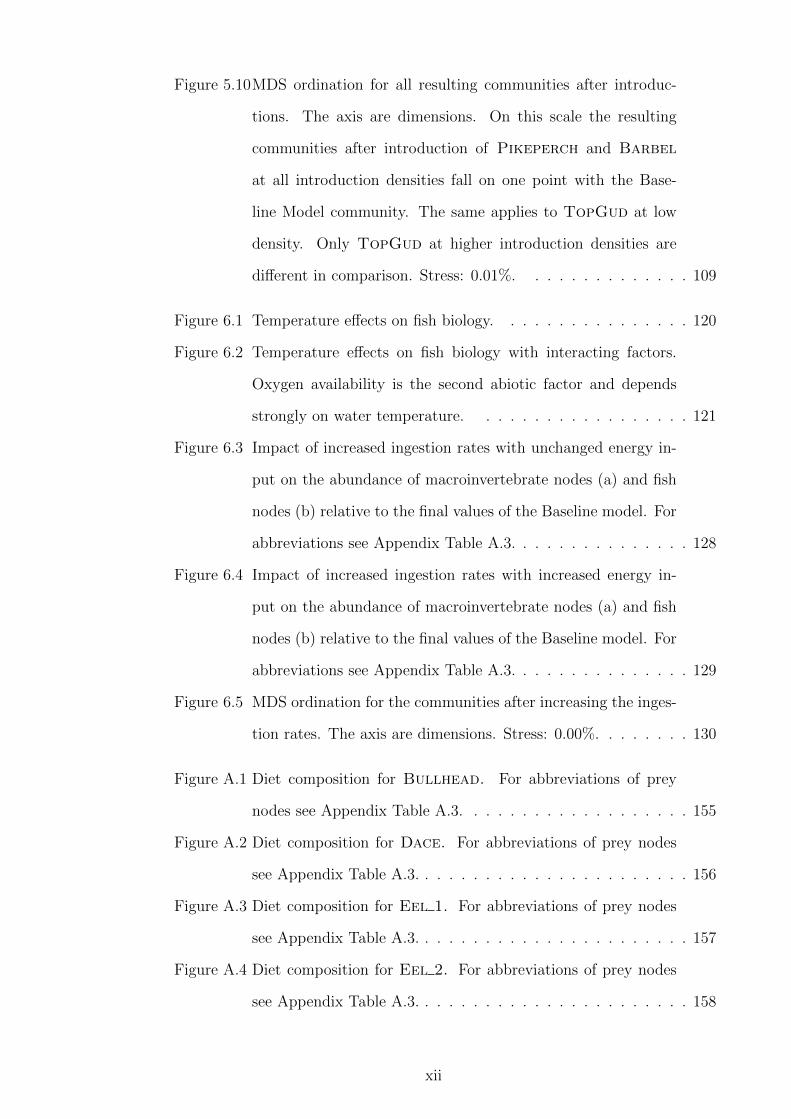
Figure 5.10MDS ordination for all resulting communities after introduc-

tions. The axis are dimensions. On this scale the resulting

communities after introduction of Pikeperch and Barbel

at all introduction densities fall on one point with the Base-

line Model community. The same applies to TopGud at low

density. Only TopGud at higher introduction densities are

different in comparison. Stress: 0.01%. . . . . . . . . . . . . . 109

Figure 6.1 Temperature effects on fish biology. . . . . . . . . . . . . . . . 120

Figure 6.2 Temperature effects on fish biology with interacting factors.

Oxygen availability is the second abiotic factor and depends

strongly on water temperature. . . . . . . . . . . . . . . . . . 121

Figure 6.3 Impact of increased ingestion rates with unchanged energy in-

put on the abundance of macroinvertebrate nodes (a) and fish

nodes (b) relative to the final values of the Baseline model. For

abbreviations see Appendix Table A.3. . . . . . . . . . . . . . . 128

Figure 6.4 Impact of increased ingestion rates with increased energy in-

put on the abundance of macroinvertebrate nodes (a) and fish

nodes (b) relative to the final values of the Baseline model. For

abbreviations see Appendix Table A.3. . . . . . . . . . . . . . . 129

Figure 6.5 MDS ordination for the communities after increasing the inges-

tion rates. The axis are dimensions. Stress: 0.00%. . . . . . . . 130

Figure A.1 Diet composition for Bullhead. For abbreviations of prey


Figure A.2 Diet composition for Dace. For abbreviations of prey nodes

see Appendix Table A.3. . . . . . . . . . . . . . . . . . . . . . . 156

Figure A.3 Diet composition for Eel 1. For abbreviations of prey nodes




xii



Figure A.6 Diet composition for Gudgeon. For abbreviations of prey


Figure A.7 Diet composition for Minnow. For abbreviations of prey nodes


Figure A.8 Diet composition for Pike1. For abbreviations of prey nodes


Figure A.9 Diet composition for Pike2. For abbreviations of prey nodes


Figure A.10Diet composition for Pike3. For abbreviations of prey nodes


Figure A.11Diet composition for Roach. For abbreviations of prey nodes


Figure A.12Diet composition for Salmon. For abbreviations of prey nodes


Figure A.13Diet composition for Stoneloach. For abbreviations of prey


Figure A.14Diet composition for Trout. For abbreviations of prey nodes


Figure A.15EcoNet generates a graph that depicts the development of the

stock values over time. This one is the output for the Baseline

Model. . . . . . . . . . . . . . . . . . . . . . . . . . . . . . . . 170

Figure D.1 MDS-ordination for removals from baseline community Autumn

’03. For abbreviations of prey nodes see Appendix Table A.3.

Stress: 10.25%. . . . . . . . . . . . . . . . . . . . . . . . . . . . 178



Stress: 9.44%. . . . . . . . . . . . . . . . . . . . . . . . . . . . 179

xiii



Stress: 10.92%. . . . . . . . . . . . . . . . . . . . . . . . . . . . 180

Figure D.4 Impact of the removal of the macroinvertebrate nodes Coleoptera,

Mollusca, Oligochaeta and Plecoptera on the abun-

dance of the remaining nodes, relative to the Baseline model.

For abbreviations of prey nodes see Appendix Table A.3. . . . . 181

Figure D.5 Impact of the removal of the macroinvertebrate nodes Diptera,

Ephemeroptera, Gammaridae and Trichoptera on the

abundance of the remaining nodes, relative to the Baseline

model. For abbreviations of prey nodes see Appendix Table A.3.182

Figure D.6 Impact of the removal of the fish nodes Bullhead, Dace,

Eel, and Gudgeon on the abundance of the remaining nodes,

relative to the Baseline model. For abbreviations of prey nodes


Figure D.7 Impact of the removal of the fish nodes Minnow, Pike, Roach

and Salmon on the abundance of the remaining nodes, rela-

tive to the Baseline model. For abbreviations of prey nodes see

Appendix Table A.3. . . . . . . . . . . . . . . . . . . . . . . . . 184

Figure D.8 Impact of the removal of the fish nodes Stoneloach and

Trout on the abundance of the remaining nodes, relative to

the Baseline model. For abbreviations of prey nodes see Ap-

pendix Table A.3. . . . . . . . . . . . . . . . . . . . . . . . . . 185

xiv

List of Tables

Table 3.1 References and locations for stomach content analysis used for

diet determination. . . . . . . . . . . . . . . . . . . . . . . . . . 49

Table 3.2 Number of extinctions for communities after additional energy

inputs were received by: firstly, only macroinvertebrate nodes;

secondly, only fish nodes; and thirdly, all nodes. In comparison,

without additional energy inputs thirteen extinctions occurred

and no extinctions occurred in the chosen Baseline Model. . . . 55

Table 4.1 Differences of the expected diversity calculated from the model

output (exp(H ′)) and the expected diversity. The expected di-

versity is calculated from the values of the Baseline model omit-

ting the value of the removed species node. For δdiv = 0: no

knock on effect after node removal; for δdiv > 0: positive knock

on effect; for δdiv < 0: negative knock on effect. . . . . . . . . 69

Table 4.2 Difference between observed and expected total energy of the

communities after the removal of a species. . . . . . . . . . . . 74

Table 5.1 Introduction abundances for Pikeperch. . . . . . . . . . . . . 91

Table 5.2 Introduction abundances for Barbel. . . . . . . . . . . . . . . 93

Table 5.3 Introduction abundances for TopGud. . . . . . . . . . . . . . 96

Table 5.4 Shannon-Diversity Index (H’ ) for the communities after the

introduction of Pikeperch at different densities. The values

in brackets are the effective number of species (true diversity,

exp (H’ )). . . . . . . . . . . . . . . . . . . . . . . . . . . . . . . 98

xv


introduction of Barbel at different densities. The values in

brackets are the effective number of species (true diversity,

exp (H’ )). . . . . . . . . . . . . . . . . . . . . . . . . . . . . . . 102


introduction of TopGud at different densities. The values

in brackets are the effective number of species (true diversity,

exp (H’ )). . . . . . . . . . . . . . . . . . . . . . . . . . . . . . . 105

Table 6.1 Increase in ingestion rates, which equivalents an increase in

temperature by 5°C, and additional energy input of each trial. . 125

Table 6.2 Shannon-Diversity Index H’ and true diversity (exp(H’ )) for

the communities after increasing ingestion rates. . . . . . . . . 127

Table 6.3 Difference between total energy of modelling trials 1–8 and the

Baseline Model. . . . . . . . . . . . . . . . . . . . . . . . . . . 131

Table A.1 Length-weight relationships for fishes and corresponding R2-

values. Column 4 shows length-weight relationships taken from

fishbase when R2 < 0.9 for the calculated length-weight relation-

ships. . . . . . . . . . . . . . . . . . . . . . . . . . . . . . . . . 151

Table A.2 Macroinvertebrate biomass data from the in 2008 conducted

survey. The mean total biomass was 12.32 g m−2. . . . . . . . . 153

Table A.3 Food web nodes, mean weight of the average individual (just

fish nodes) and starting stock values. . . . . . . . . . . . . . . . 154

Table A.4 Additional energy input that is used for removal experiments.

Additional input is the value that was added to the value ob-

tained from calculating energy demand from the metabolic rate.

The last column shows the percentage that was added to the

the calculated input based on the metabolic rate. . . . . . . . . 169

xvi

Table B.1 Different methods of stomach content analysis and their strengths

and weaknesses (Hyslop, 1980).

. . . . . . . . . . . . . . . . . . . . . . . . . . . . . . . . . . . 172

xvii

Chapter 1

Introduction

The diversity of life, or biodiversity, is a defining feature of natural ecosystems. Or-

ganisms are connected through a complex network of biological interactions, energy

fluxes and the associated physical factors that comprise the environment. Together

these govern ecosystem processes (Willis, 1997). Ecosystems differ in size, structure,

and community composition and perform essential functions such as decomposition

and waste materials processing, nutrient-recycling, and secondary production (e.g.

Cummins, 1974; Daily, 1997). Consequently, ecosystems provide important goods

and services to mankind, from the provisioning of basic needs such as food and wa-

ter up to cultural services such as recreational, intellectual and spiritual inspiration

(Costanza et al., 1997).

Since the beginning of agriculture 11,000 years ago, “humankind has increasingly

appropriated the biological resources and natural productivity of lands and seas to

support the expansion of civilisations and technologies” (Groombridge and Jenkins,

2002). However, as a result of the increase in human population, the pressures on

natural ecosystems are also increasing with direct effects on the ability of ecosys-

tems to produce goods and support their associated services (Baron et al., 2002;

Nilsson and Renofalt, 2008). Historically, pollution and land use change were the

primary factors impacting ecosystems at local and regional scales. With the recog-

nition of climate change, impacts are expected to be observed at a global scale with

1

unforeseeable consequences on biological communities (Schiedek et al., 2007; Grimm

et al., 2008). A healthy ecosystem is resilient to external disturbances without losing

its essential functions, or is able to recover relatively rapidly after being impacted

(De Leo and Levin, 1997). However, measures of ecosystem resilience to specific

disturbances are difficult to characterise despite their crucial importance to help

underpin adaptive conservation policies and management measures. Consequently,

it is becoming increasingly important to predict future global impacts on ecosystem

function (Lal, 2007; Grimm et al., 2008; Morais, 2008).

Ecosystem function is dependent on food web structure, such as the degree of com-

plexity or food chain length (Montoya et al., 2003; Thebault and Loreau, 2003). The

choice of the food web boundaries can influence food web structure, but is often not

easy to define, because ecosystems often have overlapping communities and energy

exchange (Knight et al., 2005; Power, 2006). Locality, time, distinct abiotic and

biotic factors, community structure and function have been used to define ecosys-

tem boundaries (Post et al., 2007). For instance, three broad types of ecosystems

(terrestrial, marine and freshwater) are defined. Within each of these categories,

ecosystems can be discriminated on a climatic basis, such as arctic, tropical, and

temperate. However, segregation within a single climatic zone can also be divided in

sub-ecosystems such as forest, grassland, pelagic, benthic, lentic, and lotic. All these

boundaries are structural, whereas functional boundaries can be described on the

basis of material and energy flow, species interactions and movement of organisms.

For example, steep gradients in the exchange of nutrients and energy at a certain

locality indicate a functional boundary. Often these functional boundaries are me-

diated by structural boundaries (Post et al., 2007). In particular, lakes or islands

are well-bounded systems, in both functional and structural aspects. In compari-

son, streams pose less bounded systems especially on larger temporal scales. This is

mainly due to hydrological characteristics that can cause changes in the watercourse

(structural boundary) and energy exchange with marine or terrestrial systems that

can be highly variable because of allochthonous input or nutrient transfer through

anadromous species (functional boundary). The definition of ecosystem boundaries

2

can therefore have profound consequences to the outcome of experimental or theo-

retical approaches that investigate ecosystem processes (O’Neill et al. 1986).

Freshwater ecosystems are excellent candidates for studying human induced im-

pact on ecosystem function for a number of reasons. Firstly, freshwater systems

provide important services such as drinking water, fisheries, transport routes and

recreational activities (Costanza et al., 1997; De Leo and Levin, 1997; Holmlund

and Hammer, 1999; Wilson and Carpenter, 1999; Nilsson and Renofalt, 2008). Sec-

ondly, they are experiencing increasing pressure, which is rapid and dramatic at

high altitudes and latitudes (Sala et al., 2000; Malmqvist and Rundle, 2002). Par-

ticular disturbances of riverine ecosystems include chemical and thermal pollution,

discharge regulation and water abstraction. For instance, changes in the natural

discharge regime have been shown to have a negative impact on aquatic species

diversity (Poff and Ward, 1989; Mann and Bass, 1997; Sheldon and Walker, 1997;

Dewson et al., 2007; Morais, 2008). Another increasing source of disturbance is the

introduction of non-native species, which may have major consequences for commu-

nity composition (Vander Zanden et al., 1999; Koel et al., 2005; Baxter et al., 2004;

Gozlan et al., 2010b). Thirdly, freshwater ecosystems have relatively manageable

food webs in terms of both, data availability (e.g. well quantified diet compositions)

and relatively well defined ecosystem boundaries.

For the above reasons (i.e. socio-economic importance, level of disturbance, well

established energy transfers, and manageable food web size), the development of a

dynamic food web model for a lotic freshwater system presents a realistic opportunity

to generate effective and meaningful predictions about the impact of climate change

and the introduction of non-native species on biological communities and ecosystem

function. Disturbances expected to affect freshwater ecosystems in the future are:

i) additional structural changes (e.g. river regulation, hydropower stations, land-use

change; Sheldon and Walker, 1997; Pilcher et al., 2004), ii) changes in temperature

and discharge (FSBI, 2007), and iii) biological invasions (Gherardi et al., 2008;

White et al., 2008; Gozlan et al., 2010b).

3

Structural changes alter aquatic habitats and can lead to species displacement due

to altered community composition (Morais, 2008). Human-induced disturbance on

ecosystems can be studied either by analysis of historic data, through in situ and ex

situ manipulation experiments, and/or computer simulations (Power, 1990; Hast-

ings and Powell, 1991; Green and Sadedin, 2005; Power, 2006). Although historic

long term datasets are often sparse and incomplete, these data can still provide

valuable information on ecosystem behaviour and intrinsic variation. They can de-

liver the foundation for building reliable ecosystem models, which may be used to

understand underlying mechanisms and predict future conditions (Holmes, 2006).

Manipulation experiments (i.e. large scale field experiments or small scale labora-

tory experiments) are also important for hypothesis testing and model validation

(Rykiel, 1996). Although large scale field experiments are ideal, they are expen-

sive and rare because they may cause major collateral disturbances to an ecosystem

(Lampert and Sommer, 1999) and it may be difficult to control environmental factors

(e.g. temperature) in a systematic way. Contrary, laboratory experiments offer the

opportunity to manipulate conditions precisely, but results have to be scaled up to

real ecosystems. This approach may be limited in its capacity to reproduce ecosys-

tem function and therefore in its overall relevance to test the impact of disturbances

on ecosystems (Carpenter, 1996b). Comparison of already disturbed ecosystems to

similar pristine ones can be an alternative solution to large scale field experiments.

A further and extremely promising approach is ecosystem modelling, which has be-

come increasingly prominent in recent years (Green and Sadedin, 2005). As the

available computing power limits model complexity, models should be kept as sim-

ple as possible to prevent the creation of one complex system to understand another

complex system (Voinov, 2002). According to Deming ”All models are wrong, some

models are useful” (McCoy, 1994). The modelling process itself is as valuable for the

understanding of a system as the final outcome. For example, in consideration of

questions such as: Which parameters are important and which are superfluous for

the generation of prediction? What rules or algorithms govern the system? Is the

choice of the model and parameters objective or was it made subjectively in anticipa-

4

tion of an expected answer? Although theoretical approaches are useful for finding

general rules for ecosystem behaviour, a hands on approach is needed to put conser-

vation plans into action (IPCC, 2007). More specific models for particular types of

ecosystems need to be developed and ecosystem structure, dynamics and function

have to be linked to fulfil this demand (Martinez et al., 2006; Thebault and Loreau,

2006; Thebault et al., 2007; Jordan et al., 2008). Food web simulation experiments

mimic the real ecosystem in a simplified way that allows easy and quick tests of

different conditions with a high number of replicates. Simulations are cost effective

and valuable tools for isolation of trends, which can then be verified experimentally

(Green and Sadedin, 2005). Particularly in the context of environmental change,

food web models offer a more realistic approach to identification of the impacts of

stressors compared with traditional population studies (Perkins et al., 2010).

Climate change

Global average temperatures have risen by nearly 0.8°C since the late 19th century,

with an increase of 0.2°C per decade in the last 25 years as a result of climate warm-

ing (Jenkins et al., 2008) and are predicted to increase a further 1.4–5.8°C in the

next century (IPCC, 2007). Mean annual temperatures in Southern England have

risen by 1.4–1.8°C between 1961 and 2006 (≈ 0.3°C per decade; Jenkins et al., 2008).

This has triggered species range shifts northwards and to higher altitudes in aquatic

taxa (Hickling et al., 2006). Temperature also influences the reproductive success

of aquatic organisms, since hatching success, and egg and larval development time

is strongly temperature dependent (Guma’a, 1978; Pauly and Pullin, 1988; Planque

and Fredou, 1999). Furthermore, the distribution of parasites and pathogens is af-

fected directly and indirectly (through host range shifts) by global warming and

transmission rates and virulence are expected to increase (Marcogliese, 2008). For

England and Wales, although the annual mean precipitation has not changed sig-

nificantly since the records began in 1766, in the last 45 years, heavy precipitation

events in winter became more frequent, whereas in summer they have decreased

(Jenkins et al., 2008). This trend is predicted to continue (IPCC, 2007). Changes

5

in magnitude and timing of precipitation events have direct affects on the discharge

regimes of lotic freshwater systems. Shifts in natural flow regimes have been shown

to affect biodiversity and community composition (Poff and Ward, 1989; Mann and

Bass, 1997; Sheldon and Walker, 1997; Baron et al., 2002; Dewson et al., 2007). In

a comparative study, macroinvertebrate abundance and diversity showed both in-

creases and decreases as a response to elevated and reduced discharge, whereas fish

abundance and diversity decreased in both cases (Poff and Zimmerman, 2010).

Invasive species

Invasive species have had a demonstrable impact on community structure in invaded

ecosystems (Baxter et al., 2004; Koel et al., 2005). Indeed, biological invasions and

the induced changes in the abundance of species have been shown to elicit stronger

direct and indirect effects on food webs in freshwater systems than in terrestrial or

marine systems, possibly because freshwater systems are relatively more closed sys-

tems regarding energy transfer boundaries than terrestrial or marine systems (Van-

der Zanden et al., 1999; Shurin et al., 2002; Hall et al., 2007). The introduction of

non-native species that might subsequently become invasive is facilitated via anthro-

pogenic pathways such as aquaculture and fish stocking (e.g. Copp et al., 2010a,b;

Gozlan et al., 2010b). There is some evidence that changing climatic conditions

might also benefit non-native species that have not previously been able to establish

a sustainable population due to unfavourable temperatures (Gherardi et al., 2008;

White et al., 2008). The prediction of combined impacts of climate change and

non-native species introductions on aquatic community structure is difficult, since

ecosystems are complex self-organising systems (Kay, 2000). Simultaneous changes

in several state variables can cause system behaviour that cannot be deducted from

responses to changes of single state variables (cf. Chapter 2). Temperature, dis-

charge and carbon dioxide (CO2) concentrations act on food web structure and

dynamics differently, e.g. metabolic rates, mortality and palatability (Peters, 1983;

Mion et al., 1998; Rier et al., 2002; Tuchman et al., 2002; Wright et al., 2004; Dewson

et al., 2007; Power et al., 2008).

6

Keystone species

Within a food web, species exhibit interactions of varying importance. Some ex-

ert a disproportionally large effect on food web structure (Paine, 1969a). These

“keystone” species stabilise the ecosystem, and the effect of their removal cascades

through the food web, changing species abundance of directly connected species

(through feeding links) and indirectly on to other levels of the food web (Power and

Tilman, 1996; Schmitz, 2006; Woodward et al., 2008). The ecosystem shifts into

a new state with unknown consequences on ecosystem function and services. The

identification of keystone species also constitutes a robust approach to conservation

by identifying conservation priorities, and adds to the mechanistic understanding

of the ecological processes. Potential keystone species that have been identified by

modelling approaches can then be verified in small scale exclusion experiments.

Aims and Objectives

The aim of the present study is to identify impacts of environmental change on

community structure and biodiversity using a food web modelling approach.

Objectives are:

1. Develop a quantitative dynamical food web model for a temperate chalk stream.

2. Assess impacts of single species loss on food web structure.

3. Assess impacts of single species introduction on food web structure.

4. Assess impacts of increased temperature on food web structure.

Structure of the thesis

The thesis contains seven chapters plus references and appendices. Chapter 2 is a

literature review on the characterisation of food webs, and introducing food web

7

concepts and mechanisms. Within Chapter 2, there is discussion of how the under-

standing of food web dynamics can add to the understanding of ecosystem processes

and, ultimately, ecosystem services. Chapter 3 describes the development of the

dynamic food web model that is used in the three subsequent chapters to test the

impact of the different disturbances. Chapter 3 also includes the description of the

study site from where the empirical data were collated and the description of the

modelling software. Assumptions behind the development of the “Baseline Model”

are discussed in regard to advantages and limitations. In Chapter 4, the impact

of single species removal is investigated to identify possible keystone species in the

ecosystem. Methods to assess change in community structure and ecosystem func-

tion are introduced and applied, and implications for the stability of this kind of

ecosystem are discussed. In Chapter 5, model species with different characteristics

are introduced into the food web model and the consequences on food web structure

and ecosystem function are assessed with the same methods used in the previous

chapter. Chapter 6 investigates possible impacts of climate change, concentrating

on two aspects: i) temperature rise, which has direct consequences on metabolic

rates; and ii) energy limitation as a consequence of changes in leaf litter chemistry,

triggered by rising carbon dioxide concentration in the atmosphere. For the charac-

terisation of impacts, the same methods as in the preceding chapters are used. The

general conclusion (Chapter 7) discusses possible combined impacts of the tested

disturbances and consequences on ecosystem function and services. Implications for

conservation plans and future research are explored.

8

Chapter 2

Review of food web

characterisation.

2.1 Introduction

The study of aquatic food webs has expanded greatly in recent decades. A Google

Scholar search for the term “food webs” (in “document title”) revealed that the

amount of published studies have doubled every decade since 1980. Novel, the-

oretical and empirical approaches have been developed to identify the underlying

mechanisms of the complex trophic interactions of organisms (e.g. food web topol-

ogy: Borer et al., 2002; Dunne et al., 2002a; Montoya and Sole, 2002; dynamic

approaches: De Ruiter et al., 1996; Sole and Valls, 1992; and stable isotope analysis:

Hecky and Hesslein, 1995; Vander Zanden and Rasmussen, 1999; Vander Zanden

et al., 1999). Food webs are graphical representations of nutrient or energy flows

among species or functional groups of a community, and consist of primary produc-

tion, consumption and decomposition with variable complexity (Pimm, 1982). The

structure of food webs determines ecosystem function, and Wilbur (1997) suggests

that “food webs are a central, if not the central idea in ecology”.

The study of food webs goes back to the start of the 20th century, triggered by

the need to assess fish stocks (Belgrano et al., 2005). Later, the interconnection of

9

community stability and food web complexity was investigated (MacArthur, 1955),

followed by studies that assessed the importance of single species for community

stability (Paine, 1966). Recently, advances in network analysis have given rise to

new modelling approaches in the study of ecological community stability (Berlow

et al., 2004; Dunne et al., 2004; Ulanowicz et al., 2006; Duffy et al., 2007; Jorgensen,

2007; Montoya and Yvon-Durocher, 2007; Uchida et al., 2007; Berlow et al., 2008;

Rall et al., 2008).

Healthy ecosystems, in particular aquatic systems, provide mankind with important

goods, such as food and water and with services, such as nutrient recycling (De Leo

and Levin, 1997; Holmlund and Hammer, 1999; Nilsson and Renofalt, 2008). How-

ever, the availability of these goods and services can change when an ecosystem

is permanently disturbed (De Leo and Levin, 1997; Power, 2006). Under natural

conditions, ecosystems have evolved towards an equilibrium or a set of dynamic

equilibria where, over a period of time, species diversity and biomass is maintained

(Holling, 1973; Vandermeer and Yodzis, 1999; O’ Neill, 2001). Serious disturbances

can shift the ecosystem state to a markedly different equilibrium (Vandermeer et al.,

2004), with consequences on ecosystem function. The present chapter explores the

mechanisms that influence food web structure and dynamics and how the under-

standing of these mechanisms can benefit the understanding of ecosystem processes

and ecosystem services.

2.2 Classification of organisms

In aquatic ecosystems, the flux of energy via predator-prey interaction is gener-

ally directed from small-sized, short-lived, abundant organisms with high nutrient

turnover rates to larger, long-lived, rare species that fix nutrients for longer time pe-

riods, thus making this energy unavailable (Nakazawa et al., 2007; Ings et al., 2009).

Food webs can be described not only by species interactions but also by interactions

between groups of species, such as guilds (Root, 1967; Davic, 2003) or functional

10

groups (Cummins, 1974) and the way of grouping species depends on the question

asked.

Although the terms are sometimes used synonymously, the members of a guild share

similar resources that are exploited in a similar way, whereas members of a functional

group perform similar ecosystem processes through resource exploitation (Blondel,

2003). The concept of the functional group was developed to investigate the theory

that distinct communities are constructed from the same fundamental units (Jaksic,

1981; Blondel, 2003). By exploiting the same resources, members of a guild com-

pete with each other, consequently intra-guild competition is higher than inter-guild

competition (Pianka, 1980; Jaksic and Medel, 1990). Guild members are often, but

not necessarily, closely related (Jaksic, 1981) and they form a structural component

of an ecosystem, comparable to a building block. If a member of a guild is removed,

then competition is reduced and the abundance of other guild members is expected

to change, as the remaining guild members can now exploit more of the resource.

Since functional groups are defined as performing a similar ecosystem process (e.g.

water uptake, storage of resources, pollination), they are ecologically equivalent and

add redundancy to the ecosystem (Cummins, 1974; Korner, 1993). The term redun-

dancy is used to describe species that fulfil the same function (ecological redundancy,

Walker, 1992; Lawton, 1993). The negative connotation of the term suggests that

some species are superfluous and their loss would not affect ecosystem function,

but redundancy is regarded as increasing ecosystem integrity and resilience and is

therefore valuable (Naeem, 1998). Removal of a member of the functional group

will have no effect, when redundancy is high. However, low redundancy within the

functional group can lead to altered ecosystem response (Blondel, 2003). Functional

groups are often across-taxon-assemblages, with the members showing similarities

in a functional context. During ontogeny, species can belong to different guilds and

functional groups (Werner and Gilliam, 1984). This is particularly true for lotic

systems (Cummins, 1974). Gitay et al. (1996) argue that the concept of redundancy

should be abandoned because of its uncertainties and impracticalities for conserva-

tion. The term is easily misunderstood and the difficulties arising from defining a

11

redundant species are numerous. Despite those objections to the terminology, eco-

logical redundancy can be viewed as insurance to respond to environmental change,

while sustaining dynamic ecosystem regimes (Elmqvist et al., 2003).

Size is an appealing measure by which organisms can be grouped. It is easily mea-

sured and therefore a convenient parameter for biological assessment. In aquatic

food webs, most predators are restricted to prey that are smaller than their gape

size, so body size and the organism’s possible trophic relationships are correlated.

Aquatic organisms that belong to different size categories during their life-cycle

change and expand their diet during ontogeny (Cummins, 1974). It has been sug-

gested that body size is often the stronger determinant for trophic position than

taxonomic classification (Woodward et al., 2005a; Petchey et al., 2008) and high

diet overlap among similar-sized organisms has been found (Woodward and Hil-

drew, 2002). Feeding links between species cannot only change in strength, but

also in direction. For example, large instars of caddisfly larvae prey upon alderfly

larvae, but alderfly larvae prey upon small instars of caddisfly larvae (Woodward

et al., 2005b). Predatory fish show clear ontogenetic shifts in their diet. Pelagic ro-

tifers and phytoplankton are the main food resource for newly hatched fish, but, as

the fish develops, micro-crustaceans and chironomid larvae become more important

(Nunn et al., 2007). Adult fish prey mainly on macroinvertebrates or insects (Mann

and Orr, 1969) and some become piscivorous, such as northern pike (Esox lucius)

(Mann, 1980b). Body size also seems to be linked to various other characteristics,

such as home range, population density, and metabolic rate. All of these examples

highlight the importance of including body size in models of species interactions

(Peters, 1983; Jonsson and Ebenman, 1998; Loeuille and Loreau, 2006).

Species mobility is another important factor, because mobile species create linkages

among food webs or subsets of food webs (Winemiller and Jepsen, 1998). The habitat

and home-range of an organism determine the interactions this organism can have

within the stream food web, with the intensity of the interaction determined by the

frequency and duration of encounters (Dodds, 2002). Lotic ecosystems are patchy,

being composed of different habitats such as pools, runs and riffles. Redistribution

12

of nutrients across habitats and ecosystems may have important implications for

food web dynamics (Polis et al., 1996; Polis and Hurd, 1996a,b). For example,

sessile organisms, such as net-spinning caddisflies filter by-passing food out of the

water column in contrast to Atlantic salmon (Salmo salar), which is a highly mobile

species that migrates between streams and the sea. Migratory behaviour also adds

temporal variations to food web dynamics. An entire body of research exists about

the importance of nutrient input into rivers and streams of North America by Pacific

salmon (Oncorhynchus spp.; see Cederholm et al., 1999). Once a year, adult Pacific

salmon migrate back to their birthplace to spawn and die afterwards. The carcasses

pose an important, marine-derived nutrient input into the freshwater and terrestrial

ecosystems. In general, a nested hierarchy emerges (Woodward et al., 2005a) where

patches that are inhabited by species with small home ranges are connected by more

mobile species.

2.3 Mechanisms and concepts of food webs

2.3.1 Ecosystems as self-organising systems

Ecosystems are self-organising complex systems (Kay, 2000; Sole et al., 2002) in

which organisms (i.e. parts) are interconnected through energy and material flow,

governed by positive and negative feedback loops. Emergent behaviour of self-

organising systems (a behaviour that cannot be deducted from the properties of

the parts) is a common phenomenon and at any one moment in time these systems

are defined by a set of variables, such as species diversity or productivity (i.e. state).

The sum of all available combinations of variables (i.e. the sum of states) forms the

self-organising system’s ’phase-space’ or ’state-space’. The ensemble of states, which

a dynamical system approaches from any other location in the phase-space is called

an attractor. The area of phase-space that leads to an attractor is called a domain

(or basin) of attraction. An attractor can be a single point, a periodic orbit, a limit

cycle, or a chaotic trajectory (strange attractor) (Sole and Bascompte, 2006).

13

Feedback systems, such as ecosystems, organise around attractors. As a conse-

quence, the system’s environmental situation can change, but as long as the system

state is still within the domain of attraction, the system does not perform a shift

(Kay, 2000). The positive feedback loops stabilise the system so that it maintains

its current state. When the system is moved too far from its current attractor into

a different domain of attraction, the changes that occur tend to be rapid and catas-

trophic as the system shifts. When a shift will occur and how the new state will be

characterised is hard to predict, because there are often several possible attractors.

A classic example of a system with at least two attractors is the natural process of

eutrophication, which is particularly evident in shallow lakes (e.g. Blindow et al.,

1993; Scheffer, 1990; Scheffer et al., 1993; Carpenter and Cottingham, 1997). State 1

is oligotrophy, which is defined by low productivity and transparent (clear) water, of-

ten with submerged vegetation. State 2 is mesotrophy, an intermediate state, which

is defined by moderate productivity and water turbidity. State 3 is eutrophy, which is

defined by elevated productivity, high phytoplankton density and increasingly turbid

water with little or no submerged vegetation. High nutrient input (e.g. as a result of

fertiliser use in agriculture) will shift the system from state 1 into state 3. To return

to state 1, nutrient levels have to be reduced substantially. Other than reducing the

nutrient levels, a reduction of predatory fish that feed on phytoplankton grazers,

such as Daphnia, can shift the system back to state 1. Zooplanktivore fish control

phytoplankton grazers, which control phytoplankton. Phytoplankton reduces sun-

light availability and therefore inhibits growth of submerged vegetation. A decrease

of zooplanktivore fish has a positive effect on the phytoplankton grazer population

and an (indirect) negative effect on phytoplankton. With decreasing phytoplankton

biomass, turbidity decreases and the conditions for plant growth improve. A further

increase of water clarity induced by vegetation creates the right environment for

plant growth (a positive feedback loop), therefore the system stabilises itself again.

State 3 is also stabilised by a positive feedback loop. An increase in phytoplankton

biomass increases turbidity, so phytoplankton can out-compete submerged vegeta-

tion. A similar process of eutrophication happens in flood plain hydrosystems, when

14

a side-arm is cut off from the main river and a body of standing water is created

(Amoros et al., 1987). Along with the eutrophication of the water body, growth

of aquatic plant communities reduces the open water area and organic matter in-

creases in the sediment. Herbaceous littoral plant communities follow, which are

then replaced by Salix cinerea and ultimately by forest communities. This succes-

sion is another example for a positive feedback loop, as the settlement of one plant

community (e.g. Salix ) creates the conditions for a succeeding plant community by

accumulation of biomass and evapotranspiration. This results in raised soil surface

allowing forest communities to eventually establish. However, the natural succession

can be reversed by floods, as nutrients and sediment are washed out, rejuvenating

the eutrophic side arm. Ecosystems change constantly and oscillations between dif-

ferent states are reflected in community composition with implications for ecosystem

processes and function.

How does self-organisation occur and what are its mechanisms? Ecosystems have to

follow the laws of thermodynamics (Kay, 2000), whereas the first law of thermody-

namics states that energy cannot be created or destroyed, so the total energy within

a closed system stays the same, the second law states that entropy (disorder) should

be maximised in a closed system. A simple experiment from physics illustrates the

second law. When two containers, one filled with 1000 gas atoms and the other

one empty, are connected, the system will move spontaneously towards its thermal

equilibrium with 500 molecules in each and no gradient between the containers.

This process is irreversible and also the state of maximum entropy. However, highly

organised structures are observed in biology ranging from molecules to ecosystems,

when the expected equilibrium state would be an even distribution of elemental par-

ticles. Schrodinger (1944) addressed this problem by recognising that living systems

exist in a world of energy and material fluxes. Organisation is achieved by using

energy from an outside system, reducing the entropy within, while increasing the

entropy outside. Living systems, therefore, cannot be represented as closed systems,

even in ecosystems that are sometimes regarded as closed systems, such as islands,

lakes or ponds.

15

Non-equilibrium open systems are removed from thermodynamic equilibrium by

energy and material fluxes across their boundary. Their form and structure (organ-

isation) is maintained by dissipation of energy and they are known as dissipative

structures (i.e. dissipative organisation; Kay, 2000). The theory states that they

can exist for a prolonged time away from the equilibrium in locally-produced stable

states when energy is supplied from outside (Prigogine, 1955; Nicolis, 1977). Convec-

tion, weather systems, living organisms, communities of organisms and ecosystems

are examples of dissipative structures.

The Unified Principle of Thermodynamics (Kay, 2000) states that a system will resist

being removed from the equilibrium state (a unique stable attractor) within a defined

domain of attraction. If the system is removed from its equilibrium, then gradients

are imposed on the system. As a consequence, the system will organise itself in

such a way that reduces the gradients. Further increase of the gradient will trigger

more sophisticated structures to oppose the movement away from equilibrium. This

means that the system’s ability to oppose the gradient increases the further away it

is moved from equilibrium. The propensity of systems to resist being moved from

equilibrium and to return to the equilibrium state when moved from it is referred

to as the “Restated Second Law of Thermodynamics” (Kay, 2000).

The Restated Second Law of Thermodynamics can also be formulated in terms of

“exergy”, which is a further central concept of thermodynamics (Wall, 1986; Szargut

et al., 1988; Bejan, 1997) and is a description of the quality of energy. Exergy is

a measure of the maximum capacity of the energy content of a system to perform

useful work as it proceeds to equilibrium and reflects all free energies associated

with the system (Brzustowski and Golem, 1977). The presence of energy alone does

not imply that it can be used, it is exergy that represents energy available to the

system. During any chemical or physical process, energy looses exergy irreversibly.

Exergy is a useful concept for studying non-equilibrium situations, since it serves as

a measure of the distance that a system is from its equilibrium point - the larger

the value for exergy, the further away the system is from equilibrium. If a system is

exposed to exergy from outside, then it will be displaced from equilibrium. Again,

16

to degrade exergy as efficiently as possible, the system will organise itself, opposing

further displacement. The further away a system has been moved from equilibrium,

the more opportunities arise for more sophisticated organisation to be realised, hence

the more effective the system becomes at exergy degradation (Kay, 2000).

In summary, dissipative systems exist in locally steady states away from equilibrium

and are open to energy and material flows. The non-equilibrium state is maintained

by imposed energy gradients (exergy) that, in return trigger self-organisation to op-

pose this gradient. As the system moves away from equilibrium, higher organisation

occurs and more exergy is degraded. When the system’s organisation increases, then

more possible attractors become available. The system can shift suddenly when the

present organisational structure does not dissipate exergy as efficiently as other avail-

able steady states. The process of energy and material cycling (positive feedback)

is intrinsic to dissipative structures.

These concepts can now be applied to ecosystems. If earth is regarded as an open

thermodynamic system with the sun imposing an exergy gradient, then dissipative

structures will form. These can be physical, chemical or biological, e.g. oceano-

graphic and meteorological circulation dissipate some of the incoming exergy, but

also living structures have been shown to do so. Measurements of the surface tem-

perature of terrestrial ecosystems show that more mature, complex ecosystems, such

as forests, re-radiate energy at a lower exergy level than less complex structures, such

as single species lawns (Luvall et al., 1990; Akbari et al., 1999). From an ecosystem

point of view, one can state that biotic components act together in such a way that

exergy degradation is maximised. With time, more complex organisation occurs,

the diversity grows and the organisation becomes more hierarchical (Kay, 2000).

In ecology, this phenomenon is known as ecological succession and Holling (1973)

developed the adaptive cycle metaphor (Figure 2.1; Gunderson and Holling, 2002),

whereby succession was regarded to be controlled by two phases: i) exploitation,

which is defined by rapid colonisation of a recently disturbed ecosystem and domi-

nated by r-strategists; and ii) conservation, which is defined by slow accumulation

and storage of energy and materials and dominated by K -strategists (Gunderson

17

and Holling, 2002). The latter phase shows higher organisation and exergy degrada-

tion. Holling (1973) then added two more phases to this cycle dealing with “release”

and “reorganisation” (Gunderson and Holling, 2002). Highly evolved and complex

ecosystems become more fragile to disturbances, such as forest fires, insect pests

and droughts, because biomass and nutrients are tightly bound. The release (also

called “creative destructionism”, Ω-phase) is followed by “reorganisation” (α-phase),

where soil processes minimise nutrient loss, which are reorganised to be exploited

by pioneer species. Transitions from r -phase to K -phase proceed slowly, whereas

the other transitions proceed rapidly (Gunderson and Holling, 2002). Consider a

pollution event in a stream that wipes out biota downstream of the pollution event

(release). Reorganisation is initiated not through soil processes but through the

constant supply of unpolluted water upstream of the event, which carries pioneer

species with it. With the settlement of these pioneer species (r -phase) the possibil-

ities for establishment of higher organisational structures emerge and K -strategists,

such as fish, can re-establish and the system moves into the K -phase. The same can

be applied to the floodplain example described earlier (Amoros et al., 1987). When

the side-arm of a river is cut off (release), the created water-body retains nutrients

(reorganisation), then eutrophication of the water-body allows pioneer plant species

settle (r -phase), which are slowly replaced by more complex forest communities (K -

phase). The system then re-enters the cycle when floods wash out nutrients and

existing structures are destroyed (release).

2.3.2 Ecosystem integrity, resilience and stability

As discussed earlier, food webs are characterised by individuals interconnected by

energy and material fluxes. Different trophic levels (i.e. primary production, con-

sumption, and decompostation) are dependent on the type of resource being used,

and the position of a species in a particular food web defines its trophic status

(Dodds, 2002). Species composition is determined by abiotic factors (e.g. nutrient

availability, temperature, flow), evolution and recently by the introduction of non-

native species (e.g. Scheffer, 1990; Marchetti and Moyle, 2001; Scheffer et al., 2001;

18

Figure 2.1: Holling’s (1973) adaptive cycle. After Gunderson and Holling (2002).

Daufresne et al., 2004; Baxter et al., 2005; Davey and Kelly, 2007; Dewson et al.,

2007; Mugisha and Ddumba, 2007). Therefore, different food webs are observed in

changing conditions. Exergy dissipation may be the outside constraint that triggers

forming of dissipative structures, but biota interact with their environment, influ-

encing abiotic factors that consequently generate feedback loops. This is important

because as a consequence species composition can influence the properties of an

ecosystem as much as constraints from abiotic factors.

Especially with regard to ecosystem services, species composition is important to

ensure desirable ecosystem function (Hooper et al., 2005). Riverine ecosystems are

among the most heavily impacted natural systems (Sala et al., 2000), and it is pivotal

to preserve the integrity and ensure high resilience of these ecosystems as they pro-

vide essential services (Costanza et al., 1997; Holmlund and Hammer, 1999; Wilson

and Carpenter, 1999; Baron et al., 2002). The term of ecosystem integrity is strongly

connected with a subjective human point of view of ecosystem services (De Leo and

Levin, 1997). Webster’s dictionary defines integrity as “the quality or condition of

being whole or complete.” The community structure is desired to support associated

services (Cairns, 1977) and a healthy ecosystem should resemble a natural habitat

that is expected for the region (Karr and Dudley, 1981). This definition calls for

19

a pristine ecosystem to compare other degraded ecosystems to. This is normally

achieved by characterising structural and functional aspects and comparing systems

to a hypothetical system in a pristine state. Impacts of disturbances can then be

assessed and practical approaches to secure ecosystem integrity identified (De Leo

and Levin, 1997). In context of Holling’s (1973) adaptive cycle metaphor, a pristine

system is not easily defined. Transitions between stability domains are a natural

process, but with the recognition that some of these stability domains are less likely

to supply desired ecosystem services, it might be less useful to use the terminology

“pristine” system, but rather concentrate on the necessary processes that generate

desired ecosystem services.

Resilience is a measure of the persistence of systems with multiple equilibria (Gun-

derson, 2000). A resilient system has the ability to absorb change and disturbances

while the relationships between populations and state variables are maintained

(Holling, 1973). The greater the change or disturbance that is required to transform

a system from being maintained by one set of mutually reinforcing processes and

structures to a different set, the greater is the resilience of a system (Figure 2.2).

Resilience is embedded in the dynamic properties of an ecosystem. In other words:

resilience is an emergent property of ecosystems over time and is influenced by the

interaction of structure and process that create self-organisation (Gunderson, 2000).

In physics and engineering, resilience is defined differently as the ability to quickly

return to a previous condition. In ecology, the ability of a system to return to its

original state after a temporary disturbance is called stability (Holling, 1973). The

faster the system returns and the less fluctuations are expressed, the more stable

the system would be (Figure 2.2). Stability is a measure of persistence for a system

with one global equilibrium and the measure of stability is the ‘return time’ to that

equilibrium. In summary, the choice of the measure to use depends on the type of

question investigated. Stability can only be investigated close to one equilibrium

point, to which the system state returns after a disturbance. Resilience can be ap-

plied to systems with multiple equilibria and measures the amount of disturbance a

system can absorb before a system shift occurs. In the previous examples, stability

20

and resilience were defined for a stability domain that is fixed. The shape of the

stability domain is defined by the chosen key variables, such as nutrients (Scheffer

et al., 1993; Carpenter et al., 1999), species composition (Walker et al., 1997, 1999)

or trophic relationships (He et al., 1993; Schindler et al., 1993). Those key variables

can change over time (Figure 2.3) and this is called adaptive capacity.

The terms stability and resilience have been used ambiguously in the literature

(Holling, 1973; Grimm and Wissel, 1997; Gunderson, 2000). In a review of the use

of these terminologies, 25 definitions for stability and 17 for resilience were found

(Grimm and Wissel, 1997). Altogether, 163 definitions from 70 different stability

concepts and more than 40 measures were identified. Grimm and Wissel (1997) argue

against the use of the term stability because of the many ambiguities and suggest

to rather discuss stability properties than stability itself. Furthermore, Grimm and

Wissel (1997) stressed that ecological systems are complicated and the concepts

of stability and resilience have been developed for well defined, simple dynamic

systems. Berryman (1991) disagreed with this view, and took the position that

ecological systems obey the same rules as all other dynamic systems. In summary,

the confusion over stability measures in ecosystems seems to be less due to the

complicated nature of ecosystems, but more to the arbitrary use of stability concepts.

Resource based systems like forests or fisheries are sought to be kept in a state that

guarantees optimal exploitation. This is also known as imposed resiliency (De Leo

and Levin, 1997). Dynamic processes are thought to assure ecosystem function,

so the resilience of a system to change over time is embedded in its heterogeneity

and dynamic properties (DeAngelis, 1980). A high biodiversity seems to promote

resilience and integrity (Hannah et al., 2005). Ecosystem resilience (in the sense

of their reliability to provide goods) and the relationship to biodiversity has been

considered based on concepts from reliability engineering (Naeem, 1998). In en-

gineering, the more complex a machine, the more unreliable it becomes, but the

redundant parts enhance its reliability. Naeem (1998) defined ecosystem complexity

as the number of functional groups, and redundancy is expressed as high species

richness within a functional group. Theoretical relationships of biodiversity and re-

21

Figure 2.2: Difference between ecological resilience and stability (engineering re-silience). The stability domain, which is defined by the shape of the cups, is fixedover time. The ball represents the system state. System (a) and (b) are examples ofsystems with different stability. Stability is defined by the slope of the cup. Whenthe ball is removed from equilibrium (lowest point of the cup) return time will befaster in system (b) than in (a) and fluctuations will be higher in system (a) than in(b). System (b) is the more stable system. System (c) illustrates resilience. Thereare three locally stable states displayed (multiple equilibria). State 1 is the least,state 3 is the most resilient. Only a small disturbance will shift the system statefrom state 1 into state 3, whereas a larger disturbance is needed to shift the systemstate from state 3 into state 2. The amount of disturbance that is needed to shiftthe system state is illustrated by the length of the dotted arrows.

silience have been proposed by several authors (Naeem, 1998; Figure 2.4). These

proposed relationships basically cover all possible relationships, from non-linear re-

lationships (non-linear and hump-shaped), chaotic relationships (idiosyncratic) and

monotonically increasing relationships (rivet-popping, compensating/keystone and

redundancy).

According to Holling (1973), ecosystems in the K -phase (Figure 2.1) are less resilient

than ecosystems in the r -phase (Gunderson, 2000; Gunderson and Holling, 2002).

Riverine ecosystems are constantly exposed to change (e.g. floods, droughts), so

maturity is rarely reached, except when side-arms are cut off, allowing the possibility

of forest communities to develop. Constant disturbances also mean that the system

can shift into another domain of attraction during reorganisation phase, which is

the most vulnerable of the four phases. Change in abiotic factors can be followed

by species loss or establishment of new species, which can have profound impacts on

ecosystem structure and function (e.g. Paine, 1969b; Mugisha and Ddumba, 2007).

The underlying concepts are discussed in the next section.

22

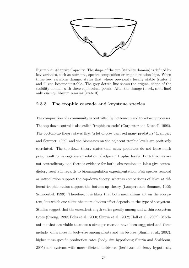
Figure 2.3: Adaptive Capacity. The shape of the cup (stability domain) is defined bykey variables, such as nutrients, species composition or trophic relationships. Whenthose key variables change, states that where previously locally stable (states 1and 2) can become unstable. The grey dotted line shows the original shape of thestability domain with three equilibrium points. After the change (black, solid line)only one equilibrium remains (state 3).

2.3.3 The trophic cascade and keystone species

The composition of a community is controlled by bottom-up and top-down processes.

The top-down control is also called ”trophic cascade”(Carpenter and Kitchell, 1996).

The bottom-up theory states that “a lot of prey can feed many predators” (Lampert

and Sommer, 1999) and the biomasses on the adjacent trophic levels are positively

correlated. The top-down theory states that many predators do not leave much

prey, resulting in negative correlation of adjacent trophic levels. Both theories are

not contradictory and there is evidence for both: observations in lakes give contra-

dictory results in regards to biomanipulation experimentation. Fish species removal

or introduction support the top-down theory, whereas comparisons of lakes at dif-

ferent trophic status support the bottom-up theory (Lampert and Sommer, 1999;

Schwoerbel, 1999). Therefore, it is likely that both mechanisms act on the ecosys-

tem, but which one elicits the more obvious effect depends on the type of ecosystem.

Studies suggest that the cascade strength varies greatly among and within ecosystem

types (Strong, 1992; Polis et al., 2000; Shurin et al., 2002; Hall et al., 2007). Mech-

anisms that are viable to cause a stronger cascade have been suggested and these

include: differences in body-size among plants and herbivores (Shurin et al., 2002),

higher mass-specific production rates (body size hypothesis; Shurin and Seabloom,

2005) and systems with more efficient herbivores (herbivore efficiency hypothesis;

23

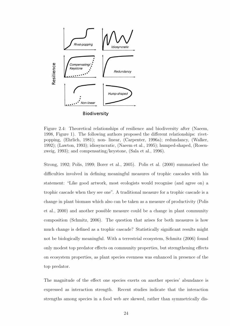
Figure 2.4: Theoretical relationships of resilience and biodiversity after (Naeem,1998, Figure 1). The following authors proposed the different relationships: rivet-popping, (Ehrlich, 1981); non- linear, (Carpenter, 1996a); redundancy, (Walker,1992); (Lawton, 1993); idiosyncratic, (Naeem et al., 1995); humped-shaped, (Rosen-zweig, 1993); and compensating/keystone, (Sala et al., 1996).

Strong, 1992; Polis, 1999; Borer et al., 2005). Polis et al. (2000) summarised the

difficulties involved in defining meaningful measures of trophic cascades with his

statement: “Like good artwork, most ecologists would recognise (and agree on) a

trophic cascade when they see one”. A traditional measure for a trophic cascade is a

change in plant biomass which also can be taken as a measure of productivity (Polis

et al., 2000) and another possible measure could be a change in plant community

composition (Schmitz, 2006). The question that arises for both measures is how

much change is defined as a trophic cascade? Statistically significant results might

not be biologically meaningful. With a terrestrial ecosystem, Schmitz (2006) found

only modest top predator effects on community properties, but strengthening effects

on ecosystem properties, as plant species evenness was enhanced in presence of the

top predator.

The magnitude of the effect one species exerts on another species’ abundance is

expressed as interaction strength. Recent studies indicate that the interaction

strengths among species in a food web are skewed, rather than symmetrically dis-

24

tributed (Berlow et al., 1999; Berlow, 1999). Few species have a high interaction

strength (exertion of a strong effect on the abundance of other species), whereas most

have weak or no detectable effects (Berlow, 1999; Emmerson and Raffaelli, 2004).

Patterning of interaction strength could have consequences for food web stability

and, consequently, community and ecosystem stability (Emmerson and Raffaelli,

2004). Emmerson and Raffaelli (2004) also found that body size of predators and

prey could be used to predict interaction strength (in this case measured as the

log-ratio measure of interaction strength; Berlow et al., 2004). The term ”interac-

tion strength” is used ambiguously in ecology and there are different measures of

link weight that are summarised with their advantages and disadvantages by Berlow

et al. (2004). The main distinction of these measures is the scale they are being used

on (property of individual link or whole system response). The absolute change in

biomass, or abundance respectively, for any species, as a response to a change in

another species abundance is called ”absolute prey response” and characterises vi-

sually dominant effects. It is a whole system response measure. Further measures

include the inverse interaction matrix (Bender et al., 1984; Yodzis, 1988), secondary

extinctions (Borrvall et al., 2000; Sole and Montoya, 2001; Dunne et al., 2002b) and

log-response ratio (Laska and Wootton, 1998; Berlow et al., 1999). Trophic cas-

cades have been shown for terrestrial, marine, and freshwater systems (Power, 1990;

Huryn, 1998; Shurin et al., 2002; Knight et al., 2005), but they seem to be strongest

in lentic freshwater systems (Shurin et al., 2002). The reason for this finding might

be that lentic freshwater systems are relatively shut off from migration. The magni-

tude of prey exchange strongly influences predator effects on prey, as a comparison

of exclusion experiments that used cages with different mesh sizes showed (Cooper

et al., 1990). Small mesh sizes hindered prey exchange and higher predator impact

was measured than in cages with larger mesh size. Predator impact can also be al-

tered by the presence of a second predator (Worsfold et al., 2009), predator identity

and predator species richness (Nilsson et al., 2008). Effects of trophic cascades can

propagate across ecosystems, e.g. fish indirectly facilitate terrestrial plant pollina-

tion in the vicinity of ponds by preying on dragonfly larvae and as a consequence less

25

adult dragonflies emerge, which prey on insect pollinators (Knight et al., 2005). In

summary, the strength of trophic cascades depends on the combination of ecosystem,

community, and species characteristics.

Single species that elicit a trophic cascade when they are removed and consequently

alter community composition (e.g. by changing plant biomass or affecting biodiver-

sity) are often referred to as keystone species. Like an arch, which is held upright

by its keystone, a keystone species is important for community stability. Originally,

Paine (1969b) defined a keystone species as ”a species of high trophic status whose

activities exert a disproportionate influence on the pattern of species diversity in a

community”. The term ”keystone” was used as a metaphor rather than as the postu-

late of a new concept (Hurlbert, 1997), although currently, the term keystone is used

widely and triggers many proposals for new definitions of the concept (Lamont, 1992;

Bond, 1993; Mills et al., 1993; Paine, 1995; Power and Mills, 1995; Folke et al., 1996;

Power and Tilman, 1996; Piraino et al., 2002; Davic, 2003). A keystone species does

not have to be a predator, but may be any species with a large effect on any aspect

of ecosystem function. This led to terms like keystone-prey, -competitor, -mutualist,

-disperser, -pollinator, -earth-mover, -habitat modifier, -engineer, -host, -processor,

-plant, and -resources, or keystone functional groups. The keystone concept is not

without criticism. There is a lack of evidence of empirical or theoretical foundation

for the existence of a natural dichotomy, which corresponds to the verbal distinction

of keystone vs. non-keystone Hurlbert (1997). However, the concept is useful to

assess a species’ ability to add stability to a food web and has gained much interest

for targeting conservation efforts efficiently (Power and Tilman, 1996; Jordan, 2009).

To be used efficiently, keystone effects need to be quantified, as assessments need

to be objective and predictive (Jordan, 2009). One aspect in the identification of

keystone species is the connectedness of the species nodes. For example, the lower

trophic level of ’wasp-waist’-like communities is connected to the higher trophic level

by only one (or very few) species, which make them energy gateways (Cury et al.,

2000). The loss of this wasp-waist species would cause a reorganisation of energy

pathways and ecosystem regime shifts (Jordan et al., 2005). Wasp-waist species are

26

often very abundant (Jordan et al., 2005) and, consequently, they are not of primary

concern, since conservation efforts are often directed towards rare species.

For water courses, the following keystone species have been identified: Power (1990)

found that in the presence of fish that prey on predatory insects and fish fry, filamen-

tous green algae are reduced to low, prostrate webs, infested with chironomids. In

fish-less exclosures, the smaller predators control chironomids, algal biomass is high

and the algal turf is covered with diatoms and cyanobacteria. Not only algal biomass

can be affected by predator prey interactions on higher trophic levels, Woodward

et al. (2008) identified European bullhead (Cottus gobio) as a keystone species of a

small chalk stream. In the investigated stream, the fish assemblage is dominated by

C. gobio and exclosure experiments revealed strong negative impacts on two prey

species- the detrivore Gammarus pulex and the algal grazer Potamopyrgus antipo-

darum. Whereas detritus processing rates were suppressed in cages containing C.

gobio, algal production did not differ (Woodward et al., 2008), so the trophic cas-

cade acted on the detrital energy pathways. Consequently, other aspects of ecosys-

tem function than plant production should be considered as well when searching for

keystone species.

The main question remains: How can trophic cascades and system regime shifts

be quantified in an objective and predictive manner? Owing to the different ways

keystone species can induce a regime shift, it is possibly best practise to assess a

combination of measures, such as changes in biodiversity, production, structural

aspects of the food web (e.g. connectivity and link density), secondary extinctions,

and dynamical aspects (e.g. energy cycling).

27

2.4 Biodiversity effects on ecosystem services and

stability

The consequences of declining biodiversity on ecosystem services and stability1 have

become of great interest in the background of accelerated species loss (Duffy, 2002).

In the 1950s, the view that more complex communities are more stable was de-

veloped. Evidence from agricultural monocultures and simple island communities

indicated that these systems were highly vulnerable to invasions when compared

to complex mainland communities (MacArthur, 1955; Elton, 1958). Elton (1958)

formulated the diversity-stability hypothesis, which states that increased biologi-

cal diversity leads to greater ecological stability and predictability and MacArthur

(1955) linked increased stability to an increase in the number of species links, which is

more likely in diverse communities. By the end of the 1950s, the positive correlation

of stability and biodiversity was treated as ecological theorem (Hutchinson, 1959).

Although supported by experimental findings (e.g. King and Pimm, 1983; Tilman

and Downing, 1994; McGradySteed et al., 1997; Naeem and Li, 1997), the theory

was seriously challenged by the analytical work of May (1972, 1973), who found

that an increase in number of species and links between them decreases stability

when the nodes are randomly connected (May, 1972). Hence, biological diversity

and complexity were not guarantors for stability, and other mechanisms and struc-

tures, which May (1973) termed ”devious strategies”, had to be found to explain

the observed diversity and complexity of ecosystems. However, natural food webs

are not connected randomly, but elicit small world behaviour, i.e. they are gener-

ally highly clustered with short path length between species and the distribution

of links is skewed (Montoya and Sole, 2002). Further food web topology studies

demonstrated the non-randomness of ecosystems (e.g. Williams and Martinez, 2000;

Dunne et al., 2002a, 2004) and increased stability of empirically consistent food

webs (Martinez et al., 2006). Omnivory might be destabilising (Pimm and Lawton,

1978) or stabilising (McCann and Hastings, 1997) and weak interactions, if the are

1The term stability is used in this section in its broadest sense, combining ecological and engi-neering resilience in its meaning, if not stated otherwise.

28

predominant, might stabilise complex communities (McCann et al., 1998). Two sets

of three species food chains that were linked by the same top predator could be sta-

bilised, when the top predator was allowed to switch preferences for its prey species

(Post et al., 2000). Furthermore, with the number of trophic levels, the frequency of

chaotic dynamics increases, but decreases with other stabilising structural properties

(Fussmann and Heber, 2002).

Although biodiversity seems to be positively correlated to ecosystem stability, it is

not essentially the driver of stability and this correlation does not necessarily extend

to stability measured on the population level (McCann, 2000). Diverse communities

potentially contain species that survive environmental disturbances and compensate

for reduced competitors (Loreau and Behera, 1999), consequently, diverse communi-

ties are potentially better ‘insured’ against environmental change and able to sustain

ecosystem dynamics in uncertain environments (Elmqvist et al., 2003). Diversity is

measured in two dimensions: functional and response diversity. Functional diversity

refers to the diversity of functional groups within an ecosystem (Elmqvist et al.,

2003). Loss of functional diversity can alter ecosystem states, e.g. loss of the top

predator (or top predator guild) can elicit a trophic cascade (Carpenter and Kitchell,

1996) and functionally diverse ecosystems have been found to be less sensitive to

invasion (Stachowicz et al., 1999; Chapin et al., 2000; Knowlton, 2001). Response di-

versity refers to the concept of redundancy within functional groups (Elmqvist et al.,

2003). Although members of a functional group may perform the same function,

their response to disturbances might be quite different. A reduction of response

diversity therefore leads to a less resilient ecosystem. For example, detrivorous

macroinvertebrates in streams are affected differently by pollution. Crustaceans

are sensitive to stream acidification, but tolerant to organical pollution, whereas

plecopterans are affected contrary (Woodiwiss, 1964; Dangles and Guerold, 1999).

Without this insurance, the process of leaf litter breakdown would stop in the case

of pollution, with consequences on higher levels of the food web, since detritus is

an important energy pathway in freshwater streams (Newman, 1991; Moore et al.,

2004). Interestingly, it has also been found that the leaf litter breakdown rates were

29

higher than expected, when shredders were cohabited, compared to isolation (Jons-

son et al., 2002). These results suggest not only the presence of response diversity,

but also functional diversity. Although the macroinvertebrates used for the exper-

iment were all shredders, their efficiency varied and in cohabitation they seemed

to complement each other. Similar results have been found for plant communities

(Walker et al., 1999) and coral reef communities (Hughes, 1994). Functional diver-

sity increases performance, since resources can be exploited more efficiently, whereas

response diversity is important to maintain ecosystem processes after perturbations

(Elmqvist et al., 2003). Consequently, slow erosion of response diversity may not

only reduce resilience, but also functionality.

In the vulnerable stage of reorganisation (Figure 2.1), response diversity might be

one of the key factors determining whether or not the system shifts towards a new

domain of attraction, which is potentially characterised by ecosystem processes that

do not support desired ecosystem services (Chapin et al., 1997). In the exploitative

phase and conservation phase, when ecosystems deliver desired services, regime shifts

seem to be less likely under conditions of high biodiversity and extensive omnivory

(Pace et al., 1999). The stabilising effect of weak interactions on complex commu-

nities (McCann et al., 1998; Neutel et al., 2002) could be negatively influenced by

biodiversity loss because of accompanying loss of weak interactions and shift towards

preponderance of strong, destabilising interactions (McCann, 2000). In summary,

biodiversity does increase stability in non-randomly interacting communities.

In the last decade, the relationship between biodiversity and ecosystem services re-

ceived growing attention, but small-scale and highly controlled experiments over

short time-periods often lack relevance to natural ecosystems and realistic extinc-

tion scenarios (Duffy, 2009). In general, biodiversity enhances ecosystem function,

specifically when the focus lies on the provision of more than one ecosystem func-

tion or service (Reiss et al., 2009). The biodiversity-ecosystem function relationship

is not simple and two mechanisms, ‘selection effect’ and ‘complementarity effect’

have been proposed to operate in combination. In the selection effect, species dom-

inance affects ecosystem processes positively or negatively according to the domi-

30

nant species’ specific traits, whereas the complementarity effect is always positive

and leads to increased total resource use by resource partitioning or positive inter-

actions (Walker et al., 1999; Loreau and Hector, 2001; Jonsson et al., 2002). The

complementarity effect is predicted to emerge over time (Pacala and Tilman, 2002),

which is confirmed in long term experiments and, simultaneously, the number of

species required to maximise function increases (Tilman et al., 2001; Hooper and

Dukes, 2004; Cardinale et al., 2007; Stachowicz et al., 2008). Dominant species

tend to influence ecosystem processes strongly (Grime, 1998; Polley et al., 2007),

and few species are needed to maintain normal ecosystem function. For example,

a common finding in experiments is that ecosystem function saturates at a species

richness level lower than that found in nature (Schwartz et al., 2000). Monocul-

tures can produce higher yields (e.g. crops, aquaculture) and, at the same time, are

harvested more efficiently (Folke, 2003; Duffy, 2009). In these systems, the focus is

on a single response variable, such as plant or fish biomass accumulation, but even

when a single species dominates a specific ecosystem service, it is unlikely to also

dominate other processes of interest. Indeed, as the considered number of ecosystem

services increases, redundancy among species decreases and the relationship between

species richness and (multivariate) ecosystem function grows stronger (Petchey and

Gaston, 2002b). This phenomenon is termed ’multivariate complementarity’ (Duffy

et al., 2003; Bracken and Stachowicz, 2006; Hector and Bagchi, 2007; Gamfeldt

et al., 2008). Moreover, rare species can make important contributions to ecosystem

processes under changing conditions (Lyons et al., 2005). It has been suggested

that the influence of diversity increases in heterogeneous conditions (Tilman et al.,

1997; Cardinale et al., 2000; Loreau et al., 2003), but most biodiversity - ecosystem

function experiments have been conducted in small plots, under highly controlled,

homogenised conditions (Duffy, 2009). Cardinale et al. (2005) found that the rela-

tionship between primary producer diversity and productivity in stream ecosystems

varies according to the disturbance history, suggesting that ecosystems that are

characterised by disturbance and high variability are more sensitive to biodiversity

loss. Additionally, the maintenance of local biodiversity at a certain level requires a

31

larger number of species at the regional scale (Duffy, 2009). Species loss negatively

affects ecosystem function, if extinction scenarios are realistic and non-random (Jon-

sson et al., 2002; Petchey and Gaston, 2002a; Ostfeld and LoGiudice, 2003; Solan

et al., 2004; Zavaleta and Hulvey, 2004). It has also been suggested that bottom-

up and top-down processes might be stronger drivers of ecosystem services than

biodiversity effects. For example, an increase in resource abundance can intensify

competition and as a consequence reduce diversity (paradox of enrichment; Huston,

1997). Contrary, the few available experimental data suggest that changing diver-

sity within trophic levels has non-trivial consequences, even within the context of

dynamic ecosystems impacted by other factors (Duffy, 2009). For example, changes

in species richness of herbivorous pond snails, had comparable or greater effects on a

range of ecosystem processes than nutrient supply or predator exclusions (Wojdak,

2005). Restoration of biodiversity in marine environments increased productivity of

fisheries and, generally, highly diverse ecosystems provided more services with less

variability (Worm et al., 2006).

The evidence suggests that stability and ecosystem services are linked to biodiver-

sity, however, in both cases, biodiversity is not the only driver. The influence of

biodiversity on ecosystem services is strongly dependent on the environmental con-

text and on the amount of desired ecosystem service. Consequently, assessments of

biodiversity alone do not permit to draw conclusions about ecosystem function and

stability.

2.5 Conclusion

The maintenance of healthy ecosystems, which consistently provide ecosystem ser-

vices and functions even in the background of environmental change, appears to

be strongly connected to the preservation of natural, diverse and dynamic commu-

nities. While ecosystem services are maintained, community compositions can be

highly variable, so the recognition of alternative domains of attraction (e.g. defined

by the ecosystem services that are provided) and drivers that cause system shifts

32

pose invaluable information for ecosystem management and conservation. Species

interact in a food web context and the structure and dynamics of these interac-

tions determine the type of ecosystem services provided and the ecosystem stability.

Therefore, the study of dynamic food webs, theoretically and empirically, gives im-

portant insights into ecosystem function and consequences of disturbances.

Although ecosystem theory seeks to identify general patterns that are valid across

different types of ecosystems, ecosystem-specific dynamics should be the focus for

predictions regarding the response to disturbances and environmental change. The

design of predictive food web models should have close resemblance to the inves-

tigated system, because randomly assembled food webs can posses properties not

observed in nature. Furthermore, the decisions made in order to build food web

models will have consequences on its behaviour. When investigating the impact of

disturbances on food webs, the type of disturbance, the response variable and a

reference state or dynamic have to be defined and spatial and temporal scales need

to be considered. Natural disturbances tend to be pulsed, whereas human induced

disturbances are often prolonged or chronic (Bengtsson et al., 2003). And in food

webs that are often subject to predictable disturbances, organisms will have evolved

to benefit from those disturbances, compared to more stable ones (Marchetti and

Moyle, 2001). The definition of a reference state tends to be more difficult, as re-

sponse variables (e.g. species abundance) tend to fluctuate naturally over time and a

decision has to be made whether or not the system has shifted into a different domain

of attraction after a disturbance. Thought has to be given to the level of descrip-

tion. When the objective is to understand ecosystem or community level dynamics,

several trophic levels should be included into the food web model. This poses diffi-

culties with regard to consistent resolution, as empirical data upon which the model

should be built, often shows higher resolution at the higher trophic levels, whereas

species are aggregated at lower trophic levels. Assessment of biodiversity effects is

made difficult with species aggregation, but is important with regard to the current

loss of biodiversity. Specifically, the interdependence of community composition,

species traits, food web dynamics and ecosystem services needs further investiga-

33

tion. Desired ecosystem services could serve as an objective function, for example, if

the objective is to maximise one service, e.g. aquaculture production, then solutions

could be achieved easily with less diverse systems. But if several ecosystem services

are of interest (e.g. regulation of ecosystem resilience, food production, nutrient

recycling), then diverse communities maximise multiple properties simultaneously

and further knowledge of food web dynamics, structure and the consequences for

ecosystem function are required.

34

Chapter 3

The aquatic food web model:

River Frome

3.1 Introduction

Fresh waters are currently subjected to numerous impacts, such as eutrophication,

climate change, toxic pollution, acidification, non-native species, over-harvesting and

habitat destruction (Covich et al., 2004). These threats can have profound conse-

quences on their ability to deliver important goods and services (Covich et al., 2004;

Woodward et al., 2005a; Balvanera et al., 2006; Schindler, 2007). How environmen-

tal stressors affect ecosystem services is determined by ecosystem resilience, which

is thought to depend on biological organisation (cf. Chapter 2). Food webs describe

communities with the focus on trophic interactions (predator-prey relationships),

with nutrient recycling and energy fluxes through the ecosystem dependent on these

interactions (e.g. DeAngelis, 1980), along with population and community dynamics

Shurin et al. (2002). Thus food web research has developed into a central issue in

ecology (de Ruiter et al., 2005). Because of the interrelationship of community dy-

namics and ecosystem function, food web analysis provides a solid approach to assess

impacts of environmental change (Ings et al., 2009). Those impacts cannot be com-

pletely understood if the investigated system contains only one trophic level or only

35

single predator-prey interactions are studied, since multilevel food webs can produce

complex behaviour and responses to disturbances can be counter-intuitive (Wilbur,

1997; Thebault and Loreau, 2003; Woodward, 2009; Woodward et al., 2010). Emer-

gent behaviours, such as resilience and ecosystem function, can only be investigated

if the system is studied at higher levels of organisation (e.g. food web or ecosystem

level). On lower organisational levels (e.g. population, single trophic level, single

predator-prey interactions), research can add to the understanding of the functional

parts of the system, but are inadequate to draw predictive conclusions to ecosystem

function and, ultimately, ecosystem services.

Food webs can be described qualitatively and quantitatively. Topological models are

a qualitative description of food webs (i.e. “who eats whom?”) with variables of in-

terest, such as connectance (number of links), and the focus is on food web patterns

and how these patterns influence food web stability (Dunne et al., 2002b; Montoya

and Sole, 2002, 2003; Ings et al., 2009). Dynamical models consider the amount of

material and energy flow over time (De Ruiter et al., 1998; DeRuiter et al., 2005).

They are a quantitative description of the system, useful to generate predictions of

changes in species abundance and test system behaviour to disturbances. Dynamical

models normally consist of a set of differential equations that characterise the rela-

tionships between the defined compartments (e.g. species, functional groups). The

Lotka-Volterra model, developed independently by Lotka (1925) and Volterra (1926),

is the simplest of the predator-prey models and is based on two-species-interactions.

Dynamic multi-species models can capture feedback loops and, therefore, emergent

properties that cannot be seen in linear systems, but they depend strongly on the

quality of the input parameters in their ability to make predictions (e.g. Baird et al.,

2009).

The alteration of food web dynamics (e.g. through loss or addition of species, change

of processing rates), can have impacts on ecosystem function, such as primary and

secondary production (Polis et al., 2000; Schmitz, 2006). How stressors impact on

biological organisation (e.g. populations, communities, food webs or ecosystems)

is still far from understood. Studies of multi-species assemblages across different

36

trophic levels are especially rare (Woodward, 2009). For example, theoretical ap-

proaches that investigate the relationship of biodiversity and ecosystem function are

ahead of available data (Thebault and Loreau, 2003, 2005, 2006). However, with-

out empirical evidence, theoretical models might not possess sufficient reality. In

the present study, this gap is attempted to be bridged by developing a food web

model based on empirical data to analyse impacts of stressors on biodiversity and

ecosystem processes (Chapters 4 to 6). To do so, a dynamical approach was chosen

in order to be able to capture processes.

Aim and objectives

The aim of this chapter is to develop a dynamical food web model based on data

from an English, temperate chalk stream, which will serve as the Baseline Model

that will be manipulated in the consequent chapters to assess the impacts of a range

of environmental changes.

Objectives are:

1. Establish species abundances from empirical data.

2. Establish diet compositions from literature.

3. Establish feeding rates.

4. Develop Baseline Model that closely resembles the natural community.

37

3.2 Material and Methods

3.2.1 Study site

The selected study site was a chalk stream in Southern England. Chalk streams

are a special type of calcareous stream found where chalk emerges on the surface of

the earth. Rainfall drains slowly downwards through the highly porous chalk until

it reaches an impervious layer below the chalk, where it accumulates, forming an

aquifier. Chalk streams rise where those aquifiers reach the surface, and their flow

originates mainly from ground water with little influence from surface runoff. The

annual hydrograph is characterised by an increasing discharge during the winter,

when the aquifiers rise and a decreasing discharge during the summer, when low

precipitation does not fill the aquifiers and they slowly empty. Normally, a substan-

tial increase in discharge can be observed in December and continues until March

and April. In dry winters, the aquifiers do not rise as much and the effects can be

observed as low discharge during summer. Low discharge exerts several ecological

effects on chalk streams, as silt accumulates and affects the growth of macrophytes,

changes the macroinvertebrate community, and influences the spawning success of

salmonid species (Berrie, 1992).

Another notable characteristic of chalk streams is a relatively stable temperature in

comparison to streams that are less influenced by ground waters. Spring water from

aquifiers in southern England emerges at about 11°C, warming the water in winter

and exhibiting a cooling effect in summer. Hence, water temperature rarely falls

below 5°C and rarely exceeds 17°C. The effect of the spring water decreases in the

lower reaches, and in prolonged periods of high temperatures (Berrie, 1992).

The chemical composition in chalk streams also remains fairly constant, and the

main nutrients for plant growth (nitrate, phosphate, potassium, and silicate) are

abundant and normally do not fall below a level where they would limit plant growth.

The combination of high level of nutrients and stable flow offers ideal conditions for

the growth of aquatic plants, such as epilithic algae and macrophytes. Annual net

38

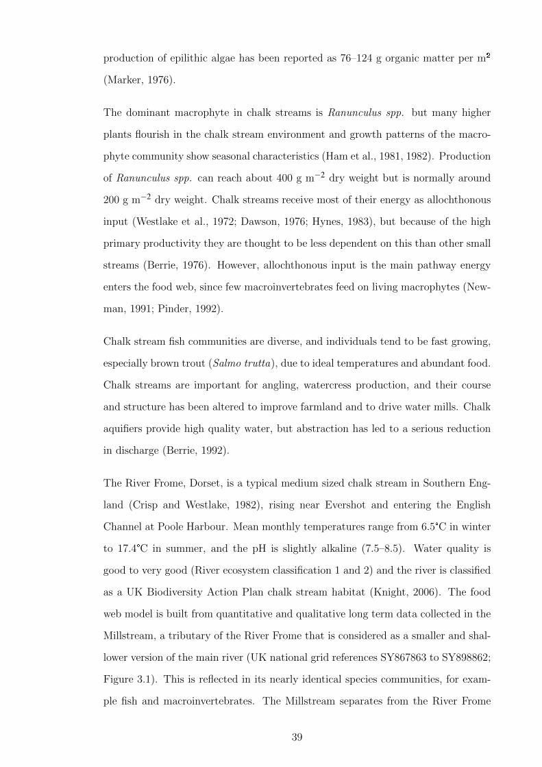
production of epilithic algae has been reported as 76–124 g organic matter per m²

(Marker, 1976).

The dominant macrophyte in chalk streams is Ranunculus spp. but many higher

plants flourish in the chalk stream environment and growth patterns of the macro-

phyte community show seasonal characteristics (Ham et al., 1981, 1982). Production

of Ranunculus spp. can reach about 400 g m−2 dry weight but is normally around

200 g m−2 dry weight. Chalk streams receive most of their energy as allochthonous

input (Westlake et al., 1972; Dawson, 1976; Hynes, 1983), but because of the high

primary productivity they are thought to be less dependent on this than other small

streams (Berrie, 1976). However, allochthonous input is the main pathway energy

enters the food web, since few macroinvertebrates feed on living macrophytes (New-

man, 1991; Pinder, 1992).

Chalk stream fish communities are diverse, and individuals tend to be fast growing,

especially brown trout (Salmo trutta), due to ideal temperatures and abundant food.

Chalk streams are important for angling, watercress production, and their course

and structure has been altered to improve farmland and to drive water mills. Chalk

aquifiers provide high quality water, but abstraction has led to a serious reduction

in discharge (Berrie, 1992).

The River Frome, Dorset, is a typical medium sized chalk stream in Southern Eng-

land (Crisp and Westlake, 1982), rising near Evershot and entering the English

Channel at Poole Harbour. Mean monthly temperatures range from 6.5°C in winter

to 17.4°C in summer, and the pH is slightly alkaline (7.5–8.5). Water quality is

good to very good (River ecosystem classification 1 and 2) and the river is classified

as a UK Biodiversity Action Plan chalk stream habitat (Knight, 2006). The food

web model is built from quantitative and qualitative long term data collected in the

Millstream, a tributary of the River Frome that is considered as a smaller and shal-

lower version of the main river (UK national grid references SY867863 to SY898862;

Figure 3.1). This is reflected in its nearly identical species communities, for exam-

ple fish and macroinvertebrates. The Millstream separates from the River Frome

39

near East Stoke and the surface area for a 200 m stretch is approximately 1200 m²

(Knight, 2006). The surrounding area is used extensively as pasture for cattle.

The riverbed is characterised by a gravel and sand substrata supporting abundant

growth of Ranunculus spp. in summer. The combination of high water quality and

chalk stream habitat supports high biological productivity in the river. The food

web of the Millstream comprises trophic links between fishes, macroinvertebrates,

macrophytes, detritus and other microorganisms (Fig. 3.2).

40

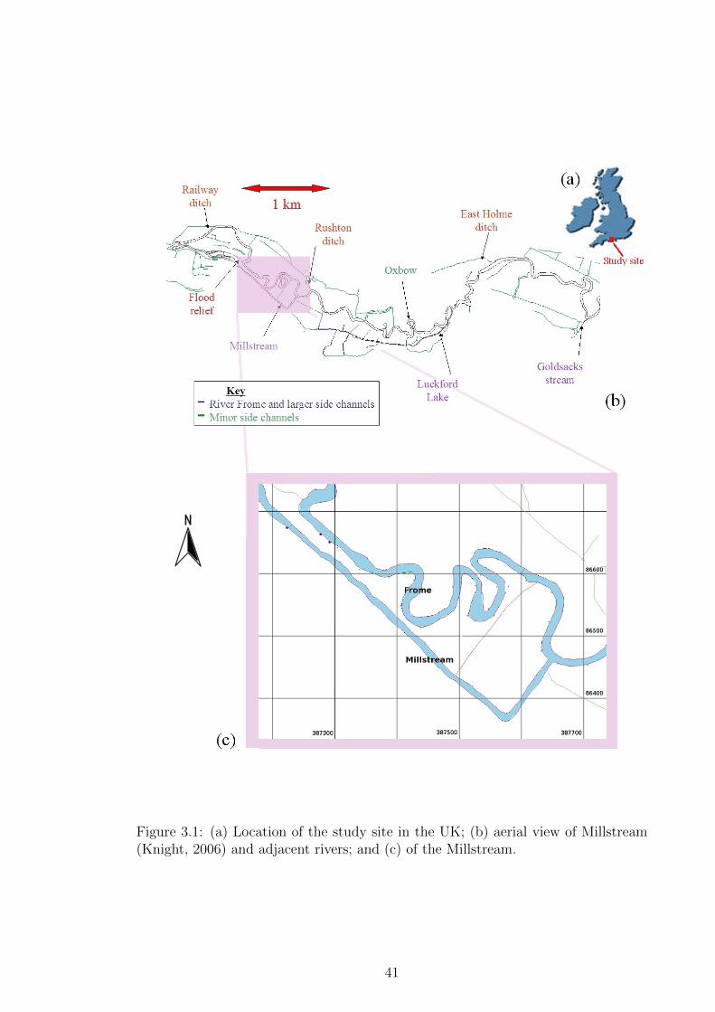
Figure 3.1: (a) Location of the study site in the UK; (b) aerial view of Millstream(Knight, 2006) and adjacent rivers; and (c) of the Millstream.

41

Figure 3.2: Schematic food web of the Millstream showing predation links amongthe main taxonomic groups. The arrows indicate the direction of energy flows.Micro- and macrophytes use dissolved nutrients and energy from the sun and detritusreceives input from all compartments, but for clarity those flows are not depicted.

42

3.2.2 Aquatic food web model

The development of the Millstream food web required certain parameters for the

chosen model to work. In general those were: i) some measure of abundance of the

compartment (i.e. species) in the form of absolute numbers, biomass or energy per

area to form the starting stock values; ii) information about how these compartments

were connected (i.e. diet composition) to form the species links; and iii) information

about the magnitude of energy flow between the compartments to characterise how

many units were transferred from one compartment to another in a given time and

space to form the energy transfer between species. To fulfil these requirements, a

combination of empirical data from the River Frome and the diet composition of

species derived from the literature was collated and processed to fulfil the demands

of the modelling approach. In particular, the chosen modelling approach required

energy values (cal) as the unit for the compartments, which were not readily available

in the literature.

Collation of data

Fish species The empirical fish data set used to build the food web was collected

by quantitative electrofishing sampling completed between 2003 and 2005 as part of

the LOCAR (LOwland CAtchment Research) programme (http://www.nerc.ac.

uk/research/programmes/locar/). Sampling was conducted four times a year in

winter, spring, summer and autumn. The sampled stretch of the Millstream was

200 m long, and was divided into 50 m stretches for quantitative assessment of the

fish communities. The 50 m sections were separated by ’stop nets’ and electrofished

using a three pass depletion method. The total area fished was 1200 m² (Knight,

2006). Captured fishes were identified to species level, and a sub-sample was mea-

sured for fork length (FL) to the nearest mm, and weighed to the nearest g. Species

specific length-weight relationships were calculated and used to obtain biomass and

energy values for the compartments used in the model (cf. Section 3.2.3). Com-

plementary length-weight relationship were collated from the literature, as for some

43

species the number of samples taken did not produce a statistical reliable length-

weight relationship (r2 < 0.9, Appendix, Table A.1). In addition, diet compositions

of the fish species were collated from the scientific literature, where extensive infor-

mation for the Frome exists (Mann and Orr, 1969; Mann, 1971, 1976a,b, 1980a,b,

1982; Mann et al., 1989; Mann and Blackburn, 1991) and were transformed into

feeding rates. Diet compositions were expressed as %-number, %-occurrence, or

%-biomass and had to be converted into energy intake per day.

Macroinvertebrate species Two surveys using the British Monitoring Working

Party (BMWP, Hawkes, 1998) methodology were carried out by the Centre for Ecol-

ogy & Hydrology (CEH) between 2002 and 2005 and provided presence/absence and

abundance characterisation of the invertebrate community of the study site. An ad-

ditional survey was carried out for this study in 2008 to provide biomass estimates

(g m−2). Samples were collected by kick-sampling method. One survey provided

abundance data identified to family level, whereas the second survey provided pres-

ence/absence data identified to species or genus. The fifty five species present from

2002 to 2005 were included in food web, although aggregated. Species frequencies

provided by the second survey were used to estimates species abundance within

families of the first survey. Finally, the 2008 survey provided data on densities (wet

weight in g m−2).

The 2008 survey was partly conducted by the author. A total of 36 samples were

taken in different habitats (e.g. gravel, Ranunculus cover) at dawn, midday and

dusk (12 samples for each time of day) on the 30th of July 2008 and the 28th of

August 2008 using a standard sampler Surber (1 min), to ensure a robust estimate

for mean biomass. The samples were kept in alcohol until the invertebrates were

sorted from debris in the laboratory; excess fluid was dried off carefully with a tissue

and the wet weight was measured. The invertebrates were not identified, but the

mean biomass per m² was calculated from the area covered by the surber net (33 cm

x 30 cm = 0.099 m²; Table A.2).

44

3.2.3 Development of the dynamical model

Introduction of the dynamical model

The dynamic simulations of the food web were run with EcoNet, a simulation and

analysis software developed at the University of Georgia (http://eco.engr.uga.edu;

Kazanci, 2007). The model, written in text format, was entered into a web interface

and then run on the external server. It was built from values for the compartments

and the flow rates between those compartments (nodes). The following parameters

were required by EcoNet to create the food web:

1. Names of nodes

2. Starting stock values for nodes

3. Flow rates between nodes

EcoNet handles simulations with two different modules. One converts the model

into differential equations; the other solves the differential equation using a method

and parameters that can be selected. The method determines how the differential

equations were solved (cf. Appendix C.1). Analysis was run with the adaptive

time-step method. Although ecosystems behave in a probabilistic manner, this

method was chosen over the stochastic method because the results did not differ,

and the calculations were solved faster with the adaptive time-step method. The

parameter Max Time Steps set the duration of the simulation and was chosen so

the final output could be assumed to be steady state. In steady state, the stock

values did not change over time- and so the network “relaxed” into its final state.

The parameter Sensitivity determined the accuracy of the numerical solution of the

differential equations. Higher values were described to be less accurate, but trial runs

with different Sensitivity values did not produce distinct results (cf. Appendix C.2).

The solution consists of a network graph, the time-course of the compartment values

and additional analysis, such as through-flow analysis, link density, connectance, and

flows at steady state (http://eco.engr.uga.edu; Kazanci, 2007).

45

The data for fish species possessed higher accuracy with regard to abundance and

diet composition than the data for macroinvertebrates. This was mainly due to

the invertebrate data not being collected with the goal to establish a food web,

but to assess biological water quality, and to diets of fish being easier to identify

to species and therefore are better known than macroinvertebrate diets. For the

dynamical model, macroinvertebrate species were organised into family groups. Al-

though there were several ways in which species could be organised (e.g. trophic

species, feeding guilds), families were used to present most diet compositions for

fish in the literature, so this grouping was adapted. This grouping may not be the

most intuitive, since families contain species with different body-size (important for

metabolic rates and prey selection), trophic position, and feeding habits (cf. Chap-

ter 2.2). Correspondingly, to counterbalance for the consequent loss of information,

the diet composition and size (in relation to occurrence) of species in each of the

families was averaged. Reliable data for microinvertebrates, microphytes, macro-

phytes and detritus were not available for the Millstream so energy inputs from

those sources were all represented as input from the environment, rather then as

nodes in the web.

Node names were written in Noun style throughout the text to indicate clearly

the species node to which they refer. When model results were put into context

with studies of natural systems, this naming convention seemed to be the most

elegant solution to avoid confusion. Dace therefore represents a node with the

mean body size and diet composition of dace (Leuciscus leuciscus). Fish nodes were

characterised by their English name, macroinvertebrate nodes by the Latin names

of family or taxa. The food web contains eight macroinvertebrate nodes and 14

fish nodes of which eel (Anguilla anguilla) and E. lucius were represented in three

nodes, respectively, to account for their changing body size and diet composition

during ontogeny (Appendix, Table A.3). The starting stock values for fish were

mean values of nine electrofishing surveys in the Millstream. The macroinvertebrate

starting values were estimated from different surveys as outlined. Energy flow rates

were based on ingestion rates for the size of the average individual of that group and

46

their diet compositions were taken from the literature. In the following section, the

application of EcoNet as a modelling tool, and the calculation of the starting stock

values, energy flow rates and parametrisation of the model are described.

Calculation of the starting stock values

Fish species For the analysis, only the data for spring, summer and autumn were

taken into account, because macroinvertebrate biomass is lower during the winter

months and correspond to a period of restricted growth for fish. To calculate the

biomass of each species and, subsequently, their energy values, fishes were initially

grouped into the following size categories (<5, 5–9.9, 10–19.9, 20–20.9 cm FL, etc),

the mean fork length in each size category calculated and then transformed into

biomass using calculated or published length-weight relationships (Appendix, Ta-

ble A.1). Overall biomass in each fish category was obtained by multiplying the

mean fish biomass by the total abundance of fish in that category. Finally, the to-

tal biomass was converted into energy per gram wet weight values, obtained from

Cummins and Wuycheck (1971). The energy values for the size categories were then

summed to obtain the starting stock values for each node, which is measured as

energy per area [cal m−2].

Macroinvertebrates species To calculate the species biomass per 100 m² (i.e.

not families), species abundances per family were transformed into dry weight using

species mean body length (Tachet et al., 2000) and associated length-weight rela-

tionships (Collins, 1992; Benke et al., 1999). The species (or species group) biomass

were subsequently converted into wet weight (1 g of wet weight = 0.23 g of dry

weight, calculated from measured overall wet weight). Cummins and Wuycheck

(1971) provided the conversion factors [cal g−1] to transform these species biomass

values into energy values [cal]. Energy values per area of single species were summed

according to families to obtain the starting stock values [cal m−2].

47

Calculation of energy flow rates

The Flow Rate characterises how much matter or energy is passed on from one

compartment to another per time step. To calculate the flow rate between the

compartments an extensive literature research was undertaken.

Fish species Diet of fish was determined from literature, where data on stom-

ach contents analysis were available. The amount of energy passed between the

compartments had to be then calculated from these data. Studies undertaken in

the Frome catchment were preferred when available (Table 3.1), and prey items

(macroinvertebrates) were determined to family level. Presuming that predators

encountered and fed on abundant prey more frequently than scarce prey, abundance

relationships of macroinvertebrates built the basis to estimate the energy transfer

from prey to predator. For some species, this may not be true (selective feeding),

but it has been shown for fish that their diet composition tends to reflect seasonal

availability of their putative prey items (Mann, 1982). Diet shifts that would oc-

cur seasonally due to availability of prey were not accounted for, but mean prey

item numbers per season across the years were used to calculate energy flow. Three

main methods to determine gut contents in fish were used in the searched literature:

number-, occurrence-, and biomass method (Appendix, Table B.1 for advantages

and disadvantages of methods). Wherever possible, number of prey items were used

to calculate energy flow, as it was the most frequent method used.

Macroinvertebrates species To establish the feeding links of macroinvertebrates,

the database of Tachet et al. (2000) was used. This used a fuzzy coding procedure in

which the relevant features of a taxon (e.g. diet) were described by the relative dis-

tribution of the assigned affinity values (from 0 - no affinity to 5 - high affinity). As

there was no detailed information available on diets of predatory macroinvertebrate,

predatory macroinvertebrate families were allowed to prey on all other macroinverte-

brate nodes. The affinity values for diet composition were converted into percentage

values to determine the proportion of energy flow, and the ingestion rate of an

48

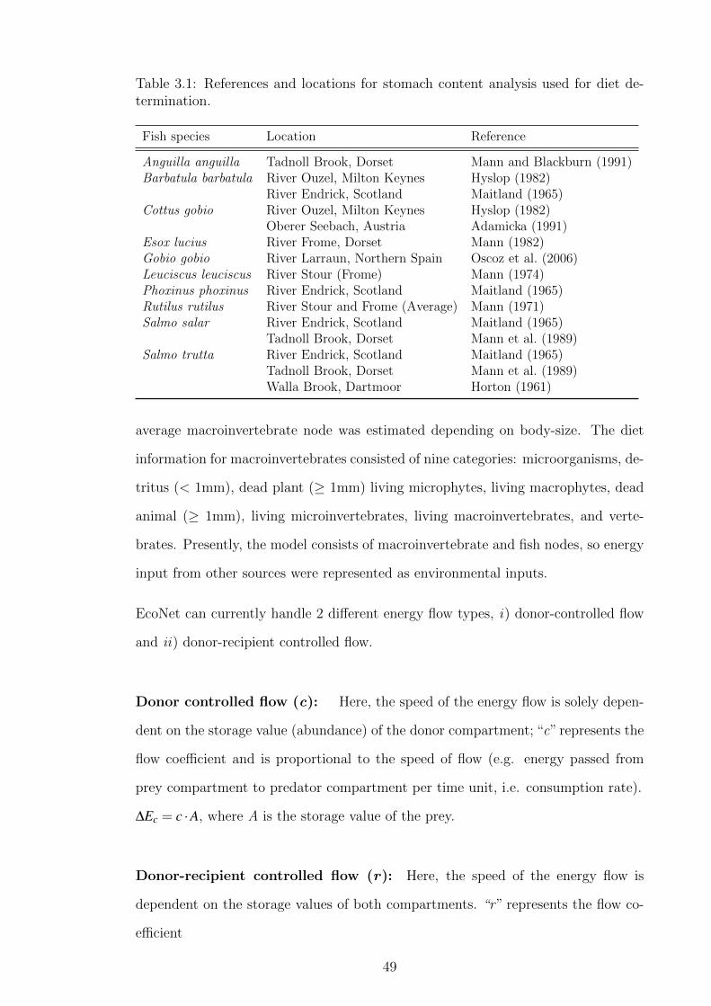
Table 3.1: References and locations for stomach content analysis used for diet de-termination.

Fish species Location Reference

Anguilla anguilla Tadnoll Brook, Dorset Mann and Blackburn (1991)Barbatula barbatula River Ouzel, Milton Keynes Hyslop (1982)

River Endrick, Scotland Maitland (1965)Cottus gobio River Ouzel, Milton Keynes Hyslop (1982)

Oberer Seebach, Austria Adamicka (1991)Esox lucius River Frome, Dorset Mann (1982)Gobio gobio River Larraun, Northern Spain Oscoz et al. (2006)Leuciscus leuciscus River Stour (Frome) Mann (1974)Phoxinus phoxinus River Endrick, Scotland Maitland (1965)Rutilus rutilus River Stour and Frome (Average) Mann (1971)Salmo salar River Endrick, Scotland Maitland (1965)

Tadnoll Brook, Dorset Mann et al. (1989)Salmo trutta River Endrick, Scotland Maitland (1965)

Tadnoll Brook, Dorset Mann et al. (1989)Walla Brook, Dartmoor Horton (1961)

average macroinvertebrate node was estimated depending on body-size. The diet

information for macroinvertebrates consisted of nine categories: microorganisms, de-

tritus (< 1mm), dead plant (≥ 1mm) living microphytes, living macrophytes, dead

animal (≥ 1mm), living microinvertebrates, living macroinvertebrates, and verte-

brates. Presently, the model consists of macroinvertebrate and fish nodes, so energy

input from other sources were represented as environmental inputs.

EcoNet can currently handle 2 different energy flow types, i) donor-controlled flow

and ii) donor-recipient controlled flow.

Donor controlled flow (c): Here, the speed of the energy flow is solely depen-

dent on the storage value (abundance) of the donor compartment; “c” represents the

flow coefficient and is proportional to the speed of flow (e.g. energy passed from

prey compartment to predator compartment per time unit, i.e. consumption rate).

∆Ec = c ·A, where A is the storage value of the prey.

Donor-recipient controlled flow (r): Here, the speed of the energy flow is

dependent on the storage values of both compartments. “r” represents the flow co-

efficient

49

∆Er = r ·A ·B), where A is the storage value of the prey, and B is the storage value

of the predator.

In most food webs, the amount of energy transferred is dependent on both: consumer

and resource abundance (Lotka-Volterra type kinetics; Kazanci, 2007). Therefore,

the donor-recipient controlled flow was chosen for all predation links between nodes.

For constant inputs from the environment and outflows (e.g. respiration, excretion),

which are only dependent on one compartment, the donor-controlled flow was used.

The following parameters were known to calculate the flow rates:

The total amount of energy a node received from all its prey items was based

on the ingestion rate I calculated from its average body weight.

The relations, i.e. how much energy is received from a single prey node, was

based on diet compositions from the literature.

The starting stock values (A: starting stock value prey; B : starting stock value

predator) was based on measured mean abundances.

Outflows were based on literature values of energy assimilation efficiency.

The metabolic rate R scales with body size, which means that small organisms have

a higher metabolic rate per gram than large organisms. For the calculations, the

ingestion rate was used, which, for poikilotherms, is ≈ 3.3 times standard metabolic

rate (Peters, 1983). Ingestion rates for all nodes were calculated as: I = 0.779W 0.82,

with W : body weight [kg] (ingestion rate for carnivorous poikilotherms, Peters,

1983) and normalised to area [m²].

The donor-recipient controlled flow calculates the change of energy (∆E) between

two nodes A and B as:

∆EAB = rAB ·A ·B, with rAB: specific flow rate between prey A and predator B ; A and

B : starting stock values of prey and predator. ∆EAB corresponds to a fraction of the

predator’s ingestion rate IB [cal m−2 d−1] as obtained from the diet compositions.

50

∆EAB = xi · IB, with 0 < xi < 1 and ∑xi = 1.

The energy flow rate rAB is therefore:

rAB ·A ·B = xi · IB

rAB =xi · IB

A ·B

Energy inputs from sources that are not represented as nodes entered the food web

from the environment and outflows that represent energy loss (except predation)

leave the food web into the environment. The environment can be interpreted as

an energy pool of infinite size, in contrast to nodes that change their stock values

dependent on in- and outflows. Energy inputs were a fraction of the ingestion rate,

if the organisms represented in that node fed on other nodes:

cenv = xi ·∆E, with 0 < x < 1 and ∑xi = 1, cenv: flow rate from the environment.

If node A receives all its energy from sources not represented as nodes, then cenv = IA,

with IA: ingestion rate for node A.

Not all energy that is transferred from one node to the next remains available. Ap-

proximately 70–95% of the energy intake is lost to the environment (e.g. respiration,

excretion) and not accumulated as biomass (e.g. growth, reproduction). The outflow

rates for all nodes were based on the assumption that 90% of the ingested energy is

lost and were calculated as:

cout f low = 0.9·IAA , with A: starting stock value of a node, IA: Ingestion rate of node A.

Model parametrisation

The model was run with the calculated starting stock values and flow rates, and the

stock values in steady state were recorded. With the adaptive time step method of

EcoNet, the parameters max time steps and sensitivity could be adjusted to alter

model performance. The influence of changing these parameters on the model output

51

was tested. While changes of the sensitivity parameter did not have an effect on the

model output, it was important to choose the max time step parameter sufficiently

large for the model to reach steady state.

To achieve a final stable state that resembled the original food web model, additional

energy inputs were given at different levels, and the final stock values were recorded.

Based on those findings, values were chosen to create the Baseline Model, which was

manipulated in the following chapters. The additional energy input came from the

environment and could also be interpreted as immigration, and not only energy input

from compartments that were not represented as nodes, such as primary producers

or detritus.

Trials were run in which the additional energy input was increased by 10, 20, 30,

40, 50, 100% of the ingestion rate. This additional input is given

1. Only to macroinvertebrate nodes.

2. Only to fish nodes.

3. To both nodes.

Statistical methods

The final stock values for each run were recorded and the distance of the result-

ing communities to the starting stock values was measured using the Bray-Curtis

dissimilarity measure. The Bray-Curtis coefficient (S jk) is a robust measure of the

similarity between two communities, and it is the recommended coefficient to anal-

yse biological data on community structure (Faith et al., 1987). It is calculated

as:

S jk = 100

1− ∑pi=1|yi j−yik|

∑pi=1(yi j+yik)

where yi j is the abundance of the ith species in the j th sample, and yik is the

abundance of the ith species in the kth sample. The coefficient equals 100 when two

52

communities are identical and it equals zero when the two compared communities are

completely different. The Bray-Curtis dissimilarity is thus calculated as 100− S jk.

The resulting matrix of coefficients was analysed using Kruskal’s non-metric Multi

Dimensional Scaling (MDS) ordination (Kruskal, 1964a,b). It is assumed for the

MDS that there should be a rank-order relationship of the similarity between the

communities, as calculated by a similarity measure, and the distance in ordination

space (Fasham, 1977). Similar communities are mapped close together, whereas

dissimilar ones are mapped further away and so the distance between two points

matches the dissimilarity value. The method was chosen because MDS has been

demonstrated as a robust unconstrained ordination method in ecology (Field et al.,

1982; Kenkel and Orloci, 1986; Minchin, 1987). Unconstrained methods are useful

to display broad patterns in a data cloud if the response variable, in this case species

abundance, is not linked to a predictor variable, such as environmental variables (An-

derson and Willis, 2003). As high dimensional data is mapped on fewer dimensions,

compromises are made in terms of accuracy in desplaying the distances between the

data points. Stress is a measure of badness of fit and needs to be considered when

interpreting the data (Kruskal and Wish, 1978). High stress indicates that distances

between data points are distorted. Generally, the amount of acceptable stress will

vary from application to application (Quist and Yona, 2004), but stress below 0.1

(10%) are considered excellent, whereas stress above 0.15 (15%) is unacceptable

(Kruskal and Wish, 1978). In the case of high stress, larger distances reflect the

data better than smaller ones, which has to be taken into account when the data is

interpreted. So even with high stress, a global pattern can still be grasped.

53

3.3 Results

The network graph produced by EcoNet (Figure 3.4) shows the direction of the

energy flows and the position of the nodes correspond to their trophic position.

Oligochaeta and Ephemeroptera received all their energy from the environ-

ment, whereas all other macroinvertebrates were predatory to some extent.

When the model was run with the calculated values, the stock values of thirteen

nodes declined to zero. The consequent rise in energy inputs had different effects

on network behaviour at different levels. Increasing energy input at the macroin-

vertebrate level caused the stock values to fluctuate before the model relaxed into

a stable state. The additional energy did not propagate to higher levels of the food

web and extinction rates remained high (Table 3.2). Trout, Gudgeon, Pike2,

Pike3, and Eel 1 were the only fish nodes still present at steady state. Extinc-

tions decreased to zero when additional energy input was given into only fish nodes.

In those cases, the model relaxed faster into steady state (≈ 1000 time steps com-

pared to 10,000 when additional energy was only given to macroinvertebrate nodes).

Pike2 and Pike3 abundance increased by 500%, whereas most other nodes showed

a decline at the highest additional input rate. Similar model outputs were observed

when additional input was given into all nodes at the same time. The main differ-

ence was that Gammaridae and Mollusca doubled in abundance. In all cases

Bullhead showed a large decline. MDS ordination (Figure 3.3) supported that

energy inputs into only macroinvertebrate nodes did not move those communities

closer to the community with the initial abundances, whereas additional input into

all nodes and only fish nodes did. Inputs around 50% into only fish nodes or all

nodes yielded communities closest to the starting values. However, direct compar-

ison of the final stock values with the initial values showed that the similarity was

not sufficient to proceed with further manipulation of the model. The additional

energy input was altered to achieve a model that resembled the initial values bet-

ter. Most of the final values that were used for further manipulation of the model

(Appendix, Table A.4) lay between 10% and 30% of the ingestion rate with a few

54

exceptions. Relatively, macroinvertebrate nodes with low abundance received much

higher additional energy inputs (Coleoptera, Plecoptera, Ephemeroptera,

Trichoptera) than the more abundant nodes, such as Gammaridae, Mollusca

and Oligochaeta. Bullhead, as the only fish node, also received a high envi-

ronmental energy input relative to its calculated ingestion rate.

Table 3.2: Number of extinctions for communities after additional energy inputswere received by: firstly, only macroinvertebrate nodes; secondly, only fish nodes;and thirdly, all nodes. In comparison, without additional energy inputs thirteenextinctions occurred and no extinctions occurred in the chosen Baseline Model.

Energy input raisedby

Macroinvertebratenodes

Fish nodes All nodes

10% 10 1 120% 10 1 130% 10 1 140% 11 1 150% 10 1 1

100% 10 1 1

55

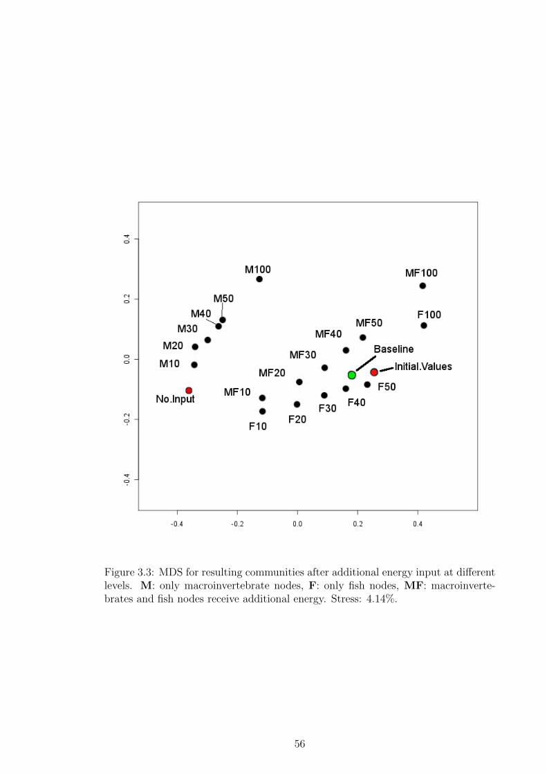
Figure 3.3: MDS for resulting communities after additional energy input at differentlevels. M: only macroinvertebrate nodes, F: only fish nodes, MF: macroinverte-brates and fish nodes receive additional energy. Stress: 4.14%.

56

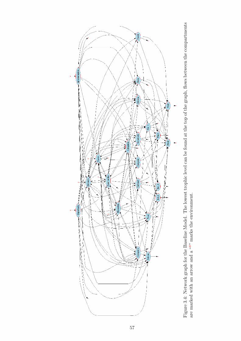
Fig

ure

3.4:

Net

wor

kgr

aph

for

the

Bas

elin

eM

odel

.T

he

low

est

trop

hic

leve

lca

nb

efo

und

atth

eto

pof

the

grap

h,flow

sb

etw

een

the

com

par

tmen

tsar

em

arke

dw

ith

anar

row

and

a“*

”m

arks

the

envir

onm

ent.

57

3.4 Discussion

The dynamic model reached a final steady state with similar abundances as the

initial starting values with additional environmental energy inputs. Without these

energy inputs, extinctions were frequent and the model would not have been suit-

able for further manipulation. The additional energy input from the environment

was justifiable since the ingestion rate used for the calculation of the energy flow

rates were approximate values and, in addition, these inputs can be interpreted as

immigration. The stabilising effect of higher energy input has also been found for

simple, three compartment energy flow models (O’Neill, 1976) where the return time

after a disturbance decreases as the rate of energy flow into the system via the au-

totroph compartment increases. Here, additional energy input into the lower levels

(macroinvertebrate nodes) alone did not move the resulting communities closer to

the initial starting values, and the number of extinctions remained high. This find-

ing suggested that the additional energy did not travel to higher levels of the food

web sufficiently to avoid the observed extinctions. A possible explanation could be

the architecture of the food web. By aggregating macroinvertebrate into trophic

species, the resolution at this level of the food web was lower than for the fish nodes.

The aggregation of macroinvertebrate species was taxonomic and although it would

have been desirable to represent these species in trophic guilds, the available diet

compositions for fish and macroinvertebrates did not allow this. Instead, the mean

diet composition and body-size of the species in a family were used to establish the

energy flows to other nodes. In the case of predatory macroinvertebrate families, all

the predatory invertebrate nodes preyed on each other, introducing feedback loops.

Those loops might be the reason for additional energy loss, since only 10% of the

ingested energy is used for growth and available to the next predator. Environmen-

tal energy input into fish nodes solved the problem and could substitute the lost

energy. If energy does not travel up the food web sufficiently because of aggregation

(less diversity, changed hierarchy), then the interpretation of changes in abundance

of macroinvertebrate nodes after manipulation of the Baseline Model is unlikely to

correspond to natural dynamics of the natural food web. Possible bottom-up ef-

58

fects could be attenuated. However, bottom up effects could be the reason for the

strong increase in Gammarus and Mollusca abundance when additional energy

was given to macroinvertebrate and fish nodes compared to the food webs, where

additional energy was only given to fish nodes. In the energy input experiments

for only fish, not only fish nodes, but the entire food web stabilised dramatically.

When additional energy was given to all nodes, top-down effects were possibly at-

tenuated, resulting in higher macroinvertebrate abundances. Bullhead declined

in all cases and required a relatively large additional energy input to produce the

Baseline Model. Compared to e.g. Dace, Bullhead has a less specialised diet and

hence should not be as dependent on the abundance of single nodes. Therefore, it

is likely that predator pressure on Bullhead let to the decline in its abundance.

Aggregation of species has been found to affect system indices of ecological network

analysis and change the global structure of the food web (Ulanowicz and AbarcaAre-

nas, 1997; Abarca-Arenas and Ulanowicz, 2002; Baird et al., 2009), particularly when

aggregations are made on the lower levels of the network (Johnson et al., 2009b).

Aggregation of detritus pools can also have serious consequences on network re-

sults (Allesina et al., 2005). These findings have consequences for the comparison of

ecosystems with different aggregations, but comparison of networks constructed with

the same constraints can still achieve useful predictions (Allesina et al., 2005). Con-

sequently, aggregated macroinvertebrate nodes should primarily be viewed as food

sources for fish nodes in the present model and predictions regarding the change in

abundance of those nodes are very general.

Increased biodiversity can lead to greater ecological stability (diversity-stability hy-

pothesis; Elton, 1958). Biodiversity is not the only factor responsible for stability in

ecosystems, as the pattern in which nodes are connected (May, 1972) and seasonal

dynamics can be important (Chapter 2). The aggregation of macroinvertebrates into

families was a simplification that disregarded the heterogeneity of a natural river food

web caused by seasonal dynamics and species diversity. Species and species aggrega-

tions were represented as ’super organisms’ that interacted only through predation

links and were evenly distributed over space. Consequently, biodiversity and het-

59

erogeneity effects on stability that are observed in natural systems (Chapter 2) may

not translate in the present food web model.

The literature that was used to determine the diet compositions spans several

decades of climate warming (Table 3.1). Fish diet can reflect macroinvertebrate

community composition to a certain extent, as more abundant prey is encountered

more often, although selective feeding has been shown as well (Mann, 1982). Poten-

tially, macroinvertebrate community composition and consequently fish diets have

already changed over the decades. Unfortunately, comparison of potential long term

changes in macroinvertebrate community composition from the diet compositions

is not possible, because diets were taken in different locations, and the influence of

location is likely to be greater than the influence of climate change.

The natural chalk stream environment is highly heterogeneous, with smaller subsys-

tems connected by larger, more mobile species (Woodward et al., 2005a). Macroin-

vertebrate communities differ in composition dependent on the substrate they live

on (e.g. gravel and Ranunculus patches). Stabilising effects that might be promoted

by heterogeneous environments and sub-communities are not captured intrinsically

in the model. Additionally, areas that are less accessible for predators, such as small

ditches or shallow riffles, might serve as refugia. Food web dynamics and growth

rates would be different in such an environment and individuals could migrate and

repopulate other areas from there. Despite the findings that species aggregation can

alter food web properties, the aggregation of nodes is general practise, especially

on the lower levels of food webs (Fath, 2004; Baird et al., 2009). Information on

energetics and diets are, in general, not as available for the base of the food web as

was the case in the present study (Baird et al., 2009). Although some of the values

for the additional energy are very high relative to the calculated ingestion rate, this

is not necessarily a problem when the model is manipulated to assess the impact of

disturbances, since the change to the Baseline Model will be assessed. Nonetheless,

these points have to be kept in mind when interpreting the results.

60

Chapter 4

Impact of species removals on

community composition

4.1 Introduction

The resilience of aquatic ecosystems to disturbances is of great concern in the back-

ground of the current rate of environmental change. Only healthy ecosystems deliver

important goods and services to society (e.g. drinking water, fisheries, and recre-

ation). A healthy ecosystem “has the ability to maintain its structure and function

over time in the face of external stress” (Costanza et al., 1997). The current ex-

ceptionally high extinction rates, which can be largely attributed to human activity

(Lawton and May, 1996), can threaten ecosystem function and therefore the supply

of ecosystem services (Chapin et al., 2000; Hooper et al., 2005; Hector and Bagchi,

2007; Gamfeldt et al., 2008; Woodward, 2009). Ecosystem function has been linked

to community structure, but how single species or communities contribute to ecosys-

tem services remains poorly understood (Larsen et al., 2005).

The resilience to perturbations and the stability of an ecosystem can be investigated

by deleting species from model food webs and investigating the consequences on

community composition (Pimm, 1980). Species deletion corresponds to a large and

persistent perturbation after which the remaining species reach a new equilibrium

61

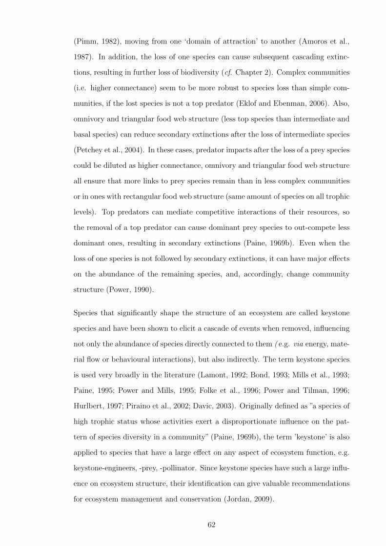
(Pimm, 1982), moving from one ‘domain of attraction’ to another (Amoros et al.,

1987). In addition, the loss of one species can cause subsequent cascading extinc-

tions, resulting in further loss of biodiversity (cf. Chapter 2). Complex communities

(i.e. higher connectance) seem to be more robust to species loss than simple com-

munities, if the lost species is not a top predator (Eklof and Ebenman, 2006). Also,

omnivory and triangular food web structure (less top species than intermediate and

basal species) can reduce secondary extinctions after the loss of intermediate species

(Petchey et al., 2004). In these cases, predator impacts after the loss of a prey species

could be diluted as higher connectance, omnivory and triangular food web structure

all ensure that more links to prey species remain than in less complex communities

or in ones with rectangular food web structure (same amount of species on all trophic

levels). Top predators can mediate competitive interactions of their resources, so

the removal of a top predator can cause dominant prey species to out-compete less

dominant ones, resulting in secondary extinctions (Paine, 1969b). Even when the

loss of one species is not followed by secondary extinctions, it can have major effects

on the abundance of the remaining species, and, accordingly, change community

structure (Power, 1990).

Species that significantly shape the structure of an ecosystem are called keystone

species and have been shown to elicit a cascade of events when removed, influencing

not only the abundance of species directly connected to them ( e.g. via energy, mate-

rial flow or behavioural interactions), but also indirectly. The term keystone species

is used very broadly in the literature (Lamont, 1992; Bond, 1993; Mills et al., 1993;

Paine, 1995; Power and Mills, 1995; Folke et al., 1996; Power and Tilman, 1996;

Hurlbert, 1997; Piraino et al., 2002; Davic, 2003). Originally defined as ”a species of

high trophic status whose activities exert a disproportionate influence on the pat-

tern of species diversity in a community” (Paine, 1969b), the term ’keystone’ is also

applied to species that have a large effect on any aspect of ecosystem function, e.g.

keystone-engineers, -prey, -pollinator. Since keystone species have such a large influ-

ence on ecosystem structure, their identification can give valuable recommendations

for ecosystem management and conservation (Jordan, 2009).

62

Within the model framework (cf. Chapter 3), the removal of a keystone species

should be identified by a significant and irreversible system shift to a new local

stable state. In contrast, redundant species would not elicit such a shift when

removed from the system. As the proposed model simulates energy flows, system

shifts that are caused by interactions, such as habitat modification or behavioural

interactions, cannot be investigated in the present study.

Assessing a system shift is not trivial. The traditional measure used to identify a

trophic cascade is a change in productivity measured as change in plant biomass

(Polis et al., 2000). However, impacts on detritus processing rates have also been

used to quantify such keystone effects (Woodward et al., 2008). These measures

are not applicable in the present study, because the dynamic food web model does

not quantify primary producers and detritus. Here, the applied measure to identify

a system shift is characterised by a significant change in community composition,

when compared to the initial food web structure. Populations naturally fluctuate

over time, while the ecosystem maintains an equal set of processes (Holling, 1973,

cf. Chapter 2). The challenge is to define a set of states (community compositions)

that reflects this natural variability and can be used as reference state or reference

dynamic. In the dynamic food web model, the starting stock values for nodes are

mean values from measurements over a three year period (cf. Chapter 3). These

measured abundances reflect the natural fluctuations in community compositions

specific to the Millstream, while the ecosystem is considered undisturbed, and thus

can be used to define the reference dynamic.

The resilience of ecosystems has been linked to biodiversity (Loreau and Behera,

1999; Elmqvist et al., 2003). A reduction of biodiversity can make an ecosystem

more vulnerable to external perturbations (Woodiwiss, 1964; Dangles and Guerold,

1999; Stachowicz et al., 1999; Chapin et al., 2000; Knowlton, 2001; Scheffer et al.,

2001; Folke et al., 2004) and reduce processing rates (e.g. leaf litter breakdown rates)

with consequences on ecosystem function (Hughes, 1994; Walker et al., 1999; Jonsson

et al., 2002). Paine (1969b) suggested a link between the removal of a keystone

species and a subsequent decline in biodiversity, because competitive interactions

63

are no longer mediated by a predator. Consequently, as processing rates cannot be

determined directly from the dynamic food web model, a decrease in biodiversity

after species removal appears to be a useful additional measure for the identification

of keystone species and for ecosystem resilience. One aspect of biodiversity loss is a

reduction in species richness (Magurran, 2004). When the loss of a species is followed

by cascading (secondary) extinctions, major changes in ecosystem properties (e.g.

changes in biomass on different trophic levels) can be observed (Thebault et al.,

2007).

Lately, an emphasis has been put on the importance to link ecosystem services and

changes in biodiversity (Thebault et al., 2007). One typical freshwater ecosystem

service concerns nutrient cycling and retention. Since the classic measure for pro-

ductivity (primary production) is not available in the dynamic food web model,

changes in secondary production can be used as a measure for ecosystem function

(Duffy, 2002). In particular, decreases in fish production could be of high economic

interest (Holmlund and Hammer, 1999). If the loss of a keystone species is followed

by a decrease in biodiversity, then this could be reflected in a decrease of secondary

production (Schlapfer and Schmid, 1999), although it has also been found that com-

petition can dampen the effect, as the biomass of the remaining, dominant species

increases, while biodiversity decreases (King and Pimm, 1983; Pimm, 1984).

Aims and objectives

The aim of this chapter is to identify the presence of keystone species in the Mill-

stream through manipulations of the dynamic food web by species removals and

measuring the extent of change in measures of species diversity, community compo-

sition and secondary production.

64


4.2.1 Manipulation of the Baseline Model - single species

removal

As in the previous chapter, the food web nodes are characterised by noun style

(Table A.3). From the Baseline Model developed in Chapter 3 (Figure 3.4), each

node was removed in turn, with the exception of Pike and Eel, where three nodes

were removed (Pike1, 2, and 3; Eel 1, 2 and 3). When a prey node was removed,

the predator covered its consumption (defined by the ingestion rate) proportionally

through higher predation rates on the remaining prey that form part of its diet. The

models were run for 5000 time-steps with a sensitivity value of 0.1 (cf. Chapter 3).

The final stock values for each species were recorded, and the resulting communities

were named after the node that has been removed. For example, the community

named “R Trout” is the resulting community after Trout removal. The Shannon

index was used to assess species diversity and compared to the Baseline Model to

assess changes. The amount of secondary extinctions was also recorded. Kruskal’s

Non-metric Multidimensional scaling (MDS) analysis was used to identify the sim-

ilarity of resulting communities (cf. Chapter 3). A system shift was identified if

the resulting community after a removal was more dissimilar than the natural vari-

ability of the system, which was defined by the measured fish abundances from the

Millstream. Finally, changes in secondary production were compared to changes in

biodiversity.

4.2.2 Diversity measure and secondary extinctions

To assess the change in diversity after species removals, the Shannon-Wiener measure

of diversity (H ′) was calculated and then converted into effective number of species

(true diversity). This conversion is advantageous because (i) the measure is intuitive,

since it reflects the number of equally common species in the community; and (ii)

65

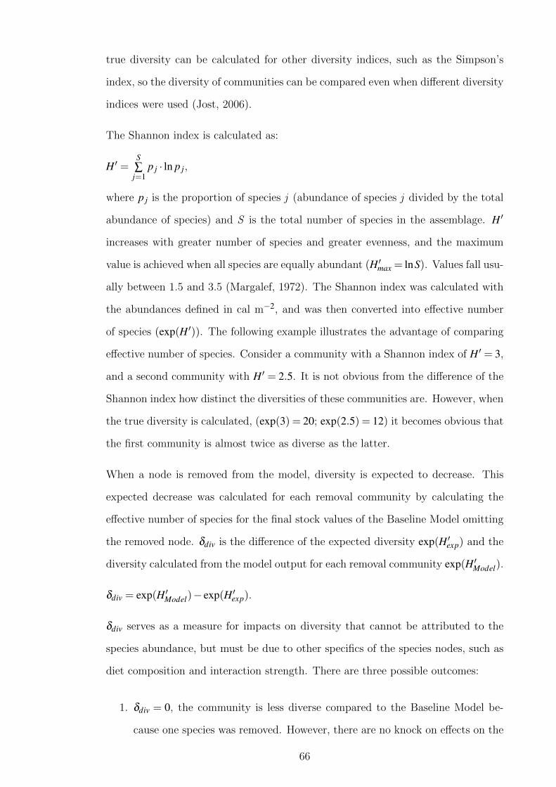
true diversity can be calculated for other diversity indices, such as the Simpson’s

index, so the diversity of communities can be compared even when different diversity

indices were used (Jost, 2006).

The Shannon index is calculated as:

H ′ =S∑j=1

p j · ln p j,

where p j is the proportion of species j (abundance of species j divided by the total

abundance of species) and S is the total number of species in the assemblage. H ′

increases with greater number of species and greater evenness, and the maximum

value is achieved when all species are equally abundant (H ′max = lnS). Values fall usu-

ally between 1.5 and 3.5 (Margalef, 1972). The Shannon index was calculated with

the abundances defined in cal m−2, and was then converted into effective number

of species (exp(H ′)). The following example illustrates the advantage of comparing

effective number of species. Consider a community with a Shannon index of H ′ = 3,

and a second community with H ′ = 2.5. It is not obvious from the difference of the

Shannon index how distinct the diversities of these communities are. However, when

the true diversity is calculated, (exp(3) = 20; exp(2.5) = 12) it becomes obvious that

the first community is almost twice as diverse as the latter.

When a node is removed from the model, diversity is expected to decrease. This

expected decrease was calculated for each removal community by calculating the

effective number of species for the final stock values of the Baseline Model omitting

the removed node. δdiv is the difference of the expected diversity exp(H ′exp) and the

diversity calculated from the model output for each removal community exp(H ′Model).

δdiv = exp(H ′Model)− exp(H ′exp).

δdiv serves as a measure for impacts on diversity that cannot be attributed to the

species abundance, but must be due to other specifics of the species nodes, such as

diet composition and interaction strength. There are three possible outcomes:

1. δdiv = 0, the community is less diverse compared to the Baseline Model be-

cause one species was removed. However, there are no knock on effects on the

66

remaining community.

2. δdiv > 0, the community is more diverse than expected. There are positive

knock on effects on the community after species removal.

3. δdiv < 0, the community is less diverse than expected. There are negative

knock on effects on the community after species removal.

Additionally, the number of secondary extinctions was recorded.

4.2.3 Comparison of the communities

The resulting communities were compared using the Bray-Curtis dissimilarity mea-

sure (see Chapter 3.2.3). The similarity matrix was calculated omitting the terms

that include the removed species, so only differences between the remaining nodes

were detectable, and not the difference caused by setting one stock value to zero.

The resulting coefficients were analysed using non-metric MDS ordination. In a sec-

ond step, the results of the MDS are put in relation to the natural variability of the

ecosystem. Recorded abundance values from the Millstream for fishes (9 measure-

ments over three years) were compared to the results from the removals. In some

of these measurements, not all fish species that are present in the Baseline Model

could be recorded and were assumed to be naturally absent. Fish abundances alone

were compared in this step, since no corresponding macroinvertebrate abundances

were available.

To assess changes in secondary production, the final stock values of all nodes were

summed for each community (EspX = ∑yi, with EspX : secondary production of com-

munity X ; yi: final stock value of node i) and compared to the secondary production

of the Baseline Model. If the removed species had no further effects on network

dynamic, then the change in secondary production would be expected to be the

difference between the secondary production of the Baseline Model and the starting

value of the removed species.

∆Energyexpected = Secondary productionBaseline−StartingValueremoved species

67

4.3 Results

After 5000 time-steps, the stock values of all models did not change further, and

the energy transfer between the compartments was fixed. Therefore, it was assumed

that all resulting communities had reached steady state.

4.3.1 Change in biodiversity secondary extinctions

The largest decline in species diversity occurred after Dace removal, followed by

Ephemeroptera, Trichoptera, Bullhead and Roach removal (Table 4.1).

Dace removal equivalented to ≈ 8% decline in true diversity, while the latter nodes

caused a decline around 5%, when compared to the expected diversity. Some re-

movals caused an increase in diversity relative to the expected diversity (Diptera,

Pike, and Eel; ≈ 5% increase). In direct comparison to the Baseline Model

(exp(H ′) = 12,7), species diversity declined by ≈ 15% after Dace removal and

≈ 10% after Ephemeroptera, Trichoptera, Bullhead and Roach removal,

whereas Diptera removal elicited no change, and Eel and Pike removals were

less diverse (≈ 9%).

None of the removals were followed by a complete secondary extinction (stock value

reaches zero). However, when extinction was defined as a decrease in abundance

of more than 95%, secondary extinction occurred twice for the same species. After

Ephemeroptera and Trichoptera removal, Roach abundance declined to 4%

of the Baseline Model abundance.

4.3.2 Comparison of the communities: MDS

In a MDS graph, communities that are similar are closer together and those that

dissimilar are further apart (Figure 4.1). Most resulting communities were close to

the Baseline Model. The communities that showed the largest decline in biodiversity

68

Table 4.1: Differences of the expected diversity calculated from the model output(exp(H ′)) and the expected diversity. The expected diversity is calculated from thevalues of the Baseline model omitting the value of the removed species node. Forδdiv = 0: no knock on effect after node removal; for δdiv > 0: positive knock on effect;for δdiv < 0: negative knock on effect.

Removed node Expected diversity Model diversity Difference δdiv

Dace 11.8 10.9 -0.9Ephemeroptera 12.6 11.9 -0.6Trichoptera 12.4 11.8 -0.6Bullhead 12.6 11.9 -0.6 δdiv < 0Roach 11.7 11.2 -0.5Gammaridae 12.9 12.7 -0.3Gudgeon 12.2 11.9 -0.2Minnow 11.7 11.6 -0.1

Trout 11.7 11.7 0.0Salmon 11.7 11.7 0.0Plecoptera 12.7 12.7 0.0 δdiv = 0Coleoptera 12.7 12.7 0.0Oligochaeta 11.9 11.9 0.0

Mollusca 11.8 11.9 0.1Stoneloach 11.9 12.1 0.1Diptera 12.2 12.7 0.5 δdiv > 0Pike 10.9 11.5 0.6Eel 10.6 11.2 0.7

Baseline Model 12.7

(Removal of Dace, Ephemeroptera, Trichoptera, Bullhead) are also found

further away from the Baseline model. Communities after Pike and Eel removals

were the the most dissimilar to the Baseline Model, and caused the largest positive

change in biodiversity. Assessment of the significance of a particular species removal

on community structure was difficult since there is no obvious threshold (distance to

the Baseline Model) that indicates a system shift. As such removals were compared

to seasonal abundance data of fish species at the study site (Figure 4.2), which

suggests that the natural variability in community composition was greater than

the changes caused by species removals. Not all species were present at all sampling

occasions, e.g. roach was not present in autumn 2004, spring 2004 and 2005. Those

three natural communities and the community after roach removal were not found

in similar locations (Figure 4.2), which suggests that the absence of a species does

69

not necessarily have a similar impact on the abundances of the remaining species.

70

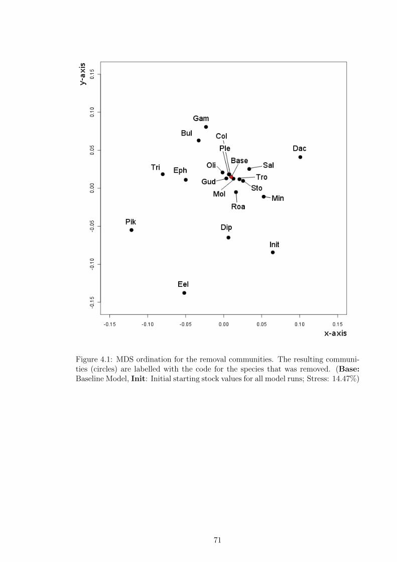
Figure 4.1: MDS ordination for the removal communities. The resulting communi-ties (circles) are labelled with the code for the species that was removed. (Base:Baseline Model, Init: Initial starting stock values for all model runs; Stress: 14.47%)

71

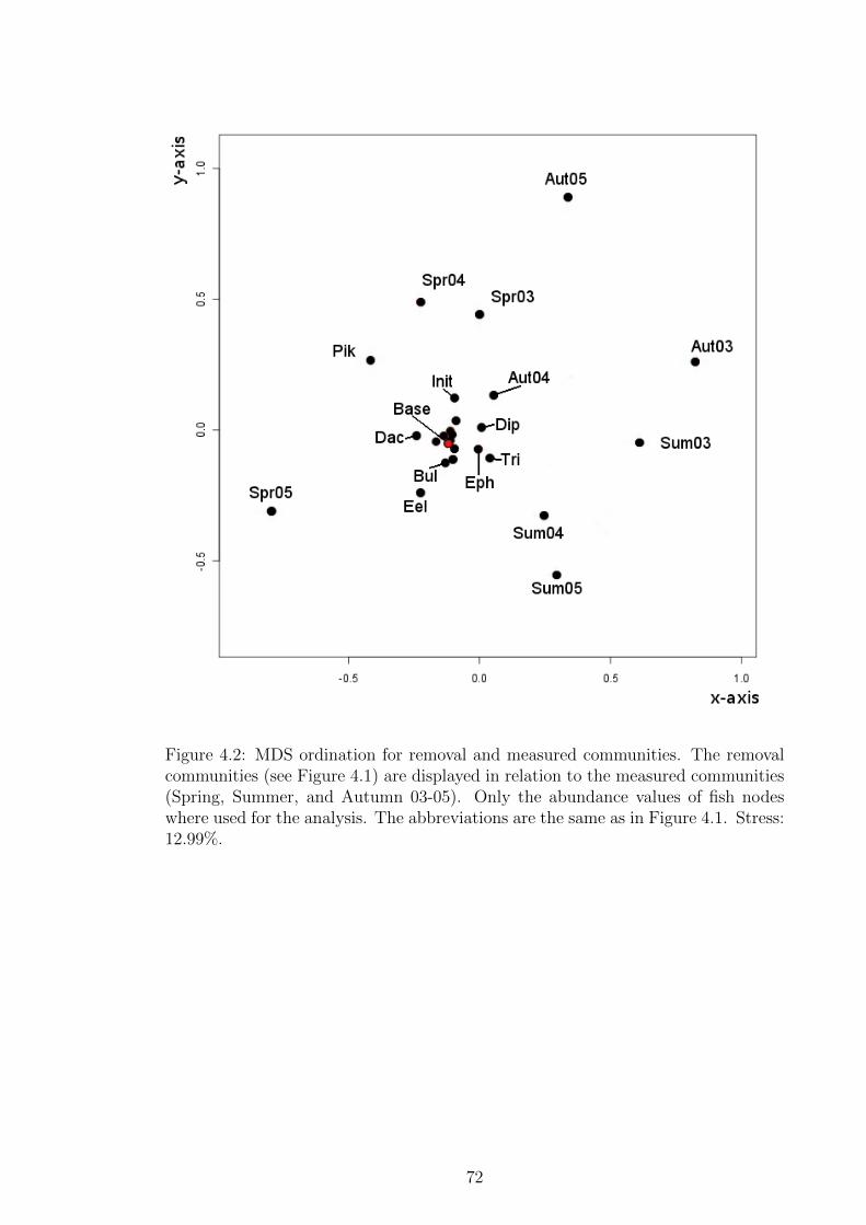
Figure 4.2: MDS ordination for removal and measured communities. The removalcommunities (see Figure 4.1) are displayed in relation to the measured communities(Spring, Summer, and Autumn 03-05). Only the abundance values of fish nodeswhere used for the analysis. The abbreviations are the same as in Figure 4.1. Stress:12.99%.

72

4.3.3 Change in secondary production

In general, secondary production was lower than expected when macroinvertebrate

nodes were removed and higher when fish nodes were removed (Table 4.2). The

largest loss of energy from the system was observed after removal of main food

sources for fish: Trichoptera, Ephemeroptera, Gammaridae and Diptera.

These results suggested that energy was not entering the food web sufficiently when

those nodes were removed. Dace, Salmon, Pike and Eel removal caused a

larger increase in secondary production than would be expected. Those removals

also caused the largest shifts according to the MDS analysis and the largest change

in diversity. The change in secondary production was not correlated to the starting

stock values of the removed species (r2 < 0.1) and no correlation was found between

secondary production and true diversity (Figure 4.3a, r2 = 0.1). There was also no

correlation found when secondary production of fish alone were compared to true

diversity (Figure 4.3b, r2 < 0.1).

73

Table 4.2: Difference between observed and expected total energy of the communitiesafter the removal of a species.

Removed node Difference betweenobserved and expected

total energy

Trichoptera -5851Ephemeroptera -4028Gammaridae -2832Diptera -2578Oligochaeta -1026Plecoptera -296Stoneloach -250Coleoptera -160Roach 13Gudgeon 38Mollusca 72Trout 84Bullhead 804Minnow 1285Eel 1923Pike 3129Salmon 5070Dace 5490

74

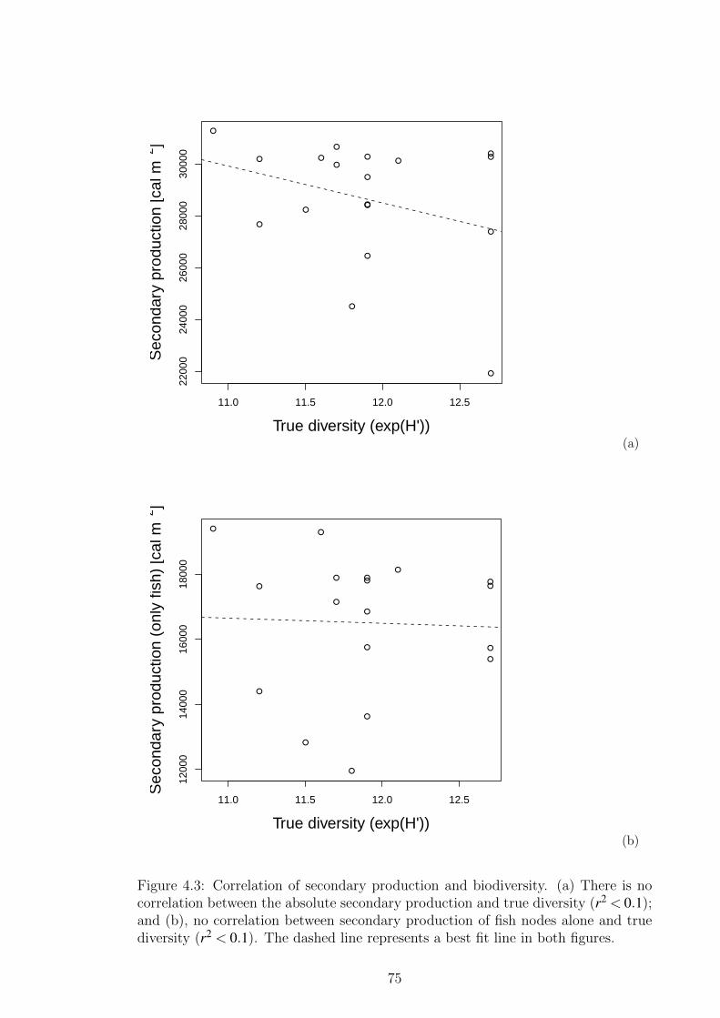
11.0 11.5 12.0 12.5

2200

024

000

2600

028

000

3000

0

True diversity (exp(H'))

Sec

onda

ry p

rodu

ctio

n [c

al m

−2]

(a)

11.0 11.5 12.0 12.5

1200

014

000

1600

018

000

True diversity (exp(H'))

Sec

onda

ry p

rodu

ctio

n (o

nly

fish)

[cal

m−2

]

(b)

Figure 4.3: Correlation of secondary production and biodiversity. (a) There is nocorrelation between the absolute secondary production and true diversity (r2 < 0.1);and (b), no correlation between secondary production of fish nodes alone and truediversity (r2 < 0.1). The dashed line represents a best fit line in both figures.

75

4.4 Discussion

Complex communities are said to be more resilient to species loss than simple ones

(Naeem and Li, 1997; Eklof and Ebenman, 2006), and this postulate is supported

by the results of the present study, which modelled a complex community. Although

some species removals had a considerable impact on community structure, none of

the removals caused a shift that was considered ecologically significant. All model

systems remained within the range of observed variability in species abundances

in the study area. For measuring ecosystem resilience, Holling (1973) proposed

that a trajectory of the cyclic behaviour of the system without forces acting on it

could serve as a reference. If forces (e.g. species removals) are now applied to the

system, then departure from this reference trajectory could be a measure of the

intensity of the forces. The fish abundances measured over the three year period

in the the Millstream were assumed to reflect the natural variability of our pristine

system, without the force of species removal acting on them. Fish abundances as

state variables were displayed in one point for every seasonal community through

MDS-ordination (Figure 4.2). These resulting nine points could now be interpreted

as boundaries for the domain of attraction. If the communities that were subject

to species removals were to fall outside these boundaries (i.e. their distance to the

Baseline Model would be larger that the distance between the Baseline Model and

the observed communities), then, per definition, a system shift would have occurred.

The results from the MDS ordination suggested that the system is resilient to single

species removal. Our model system is defined by low stability, but high resilience

(Holling, 1973). Low stability, because the abundance of species fluctuated to a cer-

tain degree within years and within seasons (Figure 4.2), with some of the fish species

not always present. High resilience, because the defined boundaries (domain of at-

traction for the ecosystem), were not crossed by the communities that experienced

species removals. Since none of the removal communities were outside the bound-

aries, it was concluded that further analysis (e.g. testing for significant differences

between the removal communities and the Baseline Model) was not adding to the

understanding of the system. Additionally, the judgement of potential system shifts

76

with the applied method was preferred to testing for significant differences between

communities because statistically significant communities might not have ecological

meaning. For example, a popular method in community ecology for analysing com-

munity similarities is ANOSIM (Analysis of similarities). However, ANOSIM was

not found suitable because, firstly, removed species enter the analysis as zero values

in contrast to the MDS, in which the removed species is omitted from the analysis

for each pair that is compared. As a consequence ANOSIM will detect differences

between the communities that are based on the species removal and not solely on

the remaining species abundances. Secondly, significant (or not significant) results

still need to be placed in a context that is ecologically meaningful, which, in this

case, was achieved by putting the results of the removals in context with the natural

variability of the system.

The results of the present study also support the findings of Eklof and Ebenman

(2006), who found that most secondary extinctions are due to direct bottom-up

effects. Here, the only secondary extinctions were caused by the removal of prey

nodes, which are a large proportion of most fish diets. Roach went extinct after

Ephemeroptera and Trichoptera removal. Although the consumption rate on

other prey nodes was raised to match the predators ingestion rate when one of its

prey species was removed, in this case the energy supply was not sufficient to support

Roach. The question remains, why only one node suffered secondary extinctions,

whereas other nodes (e.g. Bullhead and Dace) that also strongly depended on

the same prey nodes and experienced higher predator pressure did not. Roach

and Gudgeon are the only nodes that did not receive additional energy input (cf.

Chapter 3) and Gudgeon also showed a large decrease (50%) after the removal of

its main energy source (Gammaridae). The model system receives constant input

from the environment, which was needed to achieve a stable system that resembles

the natural community closely enough. The additional energy input might stabilise

the other fish nodes (O’Neill, 1976), with the effect from the removal of their prey

nodes potentially weakened.

The removal of the top predators Pike and Eel resulted in communities most

77

dissimilar to the Baseline community, although still within the proposed reference

boundaries. Predator removal can elicit a trophic cascade (Polis et al., 2000; Borer

et al., 2005; Schmitz, 2006; Hall et al., 2007) and induce system shifts (Power, 1990;

Scheffer, 1990; Carpenter and Kitchell, 1996; Scheffer et al., 2001). In our system,

Pike removal had a positive effect on Eel and vice versa and in both cases, prey

nodes were released from predator pressure and increased in abundance. In partic-

ular, Eel mainly preys on Bullhead, whereas Pike mainly preys on Minnow,

followed by Dace and Gudgeon. Eel removal was followed by a large increase in

Bullhead abundance and smaller decreases in Dace and Gudgeon abundance,

whereas Pike removal was followed by an increase in Gudgeon, Minnow and

Dace and a decrease in Bullhead. These results are in accordance with findings

that a second predator can mediate predator impact (Worsfold et al., 2009) and that

more diverse predator guilds are more effective in exploiting the available resources

(Nilsson et al., 2008). A dampening effect of predator diversity on trophic cascades

has also been found for terrestrial systems (Finke and Denno, 2004). Comparative

studies of predator removal experiments in cages found that the strength of predator

impacts was dependent on the magnitude of prey exchange rates between the cage

and the surrounding environment and the spatial scale of experiments (Cooper et al.,

1990; Englund, 1997). Smaller mesh size of the cages hindered prey exchange and

stronger trophic cascades could be observed, whereas larger mesh sizes allowed prey

exchange and observed trophic cascades were weak (Cooper et al., 1990). When the

additional energy input is interpreted as immigration, observed predator impacts

could potentially be dependent on the magnitude of these inputs.

Macroinvertebrate and fish node removals had different effects on secondary pro-

duction. Whereas, macroinvertebrate removal generally resulted in lower secondary

production, fish removal resulted in higher secondary production. In the present

study, diversity could not be linked to secondary production as a measure of ecosys-

tem function.

The Millstream food web model can be described as resilient to single species re-

moval, although some impacts have been shown, in particular after prey removal.

78

Fath (2004) found that network parameters are affected by network size, i.e. they are

scale dependent, which has direct consequences on the selection of system boundaries

and aggregation of species. Aggregated nodes, such as macroinvertebrate families

in the present study, can also have an effect on system indices that define resilience

(Cohen et al., 1993; Abarca-Arenas and Ulanowicz, 2002; Johnson et al., 2009b).

Detailed information on high level consumers with aggregation lower in the food

web may overestimate ecosystem resilience (Pinnegar et al., 2005). Consequently

the model’s predictive value should increase with further resolution of the macroin-

vertebrate nodes. Not all members of the macroinvertebrate families share the same

feeding patterns, which has been averaged for the present study. At the moment,

macroinvertebrate nodes can merely be interpreted as food sources for fish. The

difficulty in representing macroinvertebrate nodes in greater detail, comes from a

lack of available data. However, the results emphasised the influence of prey nodes

on secondary production with relevant consequences for conservation, since it high-

lights the importance to direct management efforts towards ensuring a healthy food

supply for fishes. In addition, the influence of top predators on community compo-

sition was confirmed. Contrary to Paine’s (1969b) definition of a keystone species,

diversity increased relatively after the removal of one predator, but it still has to

be confirmed, if the same result is found when both predators are removed simul-

taneously, since Paine’s model ecosystem only consisted of one top predator. It is

likely that top predators are the first to go extinct as a response to environmental

change (Petchey et al., 1999; Duffy, 2003) and future research should incorporate

sequential species deletions that are ecological meaningful to test further scenarios

that might cause significant shifts. In summary, it was not possible to identify one or

more keystone species with the applied modelling approch for this ecosystem. None

of the removals caused a significant and irreversible system shift. However, some

removals caused larger dissimilarities in community composition and biodiversity

than others, confirming that species influence the shaping of community structure

differently. The lack of keystone species could have several reasons. Firstly, the

ecosystem has a high redundancy on all levels, which makes the loss of a single

79

species less dramatic. Secondly, the discussed factors that might have artificially

increased stability in the model system (aggregation, additional energy input) could

have disguised possible shifts. Thirdly, species removal might impact more severly

on other aspects of ecosystem function than secondary production, which were not

investigated in the current study.

80

Chapter 5

Impact of non-native species

introductions on food web

structure and biodiversity

5.1 Introduction

In the last 30 years, with growing global trade the rate of fish introduction has

doubled, and with it the risk of impact on freshwater ecosystems (Gozlan et al.,

2010b). The main introduction pathways are aquaculture (De Silva et al., 2006),

improvement of wild stocks (Ogutuohwayo and Hecky, 1991; Gherardi et al., 2008),

ornamental fish trade (Copp et al., 2005b, 2010b; Keller and Lodge, 2007; Zieba et al.,

2010), and bio-control (Kumar and Hwang, 2006), but also accidental introductions

have been reported (Holcik, 1991; Gozlan et al., 2002). There is a direct link between

human population density and live fish imports (Copp et al., 2007, 2010a), indicating

that economic and social drivers are a main driver of propagule pressure of fish

introductions (Gozlan, 2008a,b; Copp et al., 2010a). Colonisation processes are no

longer restricted to natural dispersal events that are inhibited by natural barriers,

rather human induced movements over large spatial areas are increasingly common

(Rahel, 2007). When a fish is introduced into a suitable ecosystem for their biological

81

and ecological requirements, their establishment is strongly correlated to propagule

pressure (number and frequency of introductions; Copp et al., 2007; Gozlan, 2008b;

Copp et al., 2010a). The adverse impacts of introduced species can be categorised

into ecological and socio-economic effects, though the socio-economic benefits are

generally perceived to outweigh the ecological adverse effects (http://www.fao.

org/fishery/en).

Aquaculture and ornamental fish trade (Copp et al., 2005a, 2010b; Rixon et al.,

2005; Duggan et al., 2006; Zieba et al., 2010) are driven by the associated financial

benefits of these businesses. Aquaculture is probably the fastest growing business

in the food sector (FAO, 2008). Almost half of the world’s food fish is presently

produced in aquaculture (Duarte et al., 2009). The U.K.’s aquaculture production

showed a steady increase from 30 to 888 tonnes per year between 1950 and 1978,

followed by a massive rise to the current 174 203 tonnes per year, with a total value

of A£581 million (FAO, values from 2007). The recreational fishing industry across

Europe is worth over A£22 billion per year (Arlinghaus et al., 2002; Cooke and

Cowx, 2004). In Great Britain, an estimated 3.3 million recreational anglers spent

a total of A£3.3 billion pounds annually on fishing (NRA, 1994; Lewis, 2004). The

international ornamental fish industry is worth an estimated A£9.4 billion(FAO,

2008), including wages, retail sales and associated materials. Jobs are created in

export and import countries, and especially developing countries rely on harvesting

ornamental species in areas where there are little opportunities for other sources of

income.

Except for intentional stocking of recreational fisheries, non-native fish used in aqua-

culture and for ornamental purpose tend to be kept in closed systems with relatively

high bio-security measures in place to limit escape and subsequent dispersal. De-

spite these measures, escapees (accidental and intentional) are a relatively common

phenomenon, increasing the likelihood of their colonisation and subsequent estab-

lishment (Copp et al., 2005d). Although ornamental warm water species (thermal

optima > 28°C) are unlikely to be able to establish in the wild in temperate re-

gions, cold water (thermal optima < 20°C) and cool-water (thermal optima between

82

20 to 28°C) fishes may survive and establish, particualarly in Southern England

(Britton et al., 2010a). Fish that survive, but do not establish due to temperature

constraints, may benefit if thermal inhibitions dimish through climate warming and

so their establishment may still occur but be subject to a lag phase (Britton et al.,

2010a). Where non-native escapees have dispersed into the wild, colonised new wa-

ters and established sustainable populations, adverse ecological consequences may

be incurred (Gozlan et al., 2010b). It is thus important to develop predictions of

potential ecological impacts following their introductions. The key ecological im-

pacts that may be associated with non-native fish in the environment are: habitat

degradation (Miller and Crowl, 2006), hybridisation (Hanfling et al., 2005), disease

transmission (Blanc, 1997; Gozlan et al., 2005; Gozlan, 2008b), and impacts on food

web structure though predation and competition (Townsend, 2003).

There is an ongoing debate on how an ecological impact through non-native fish

introductions may be best defined and measured, since impacts are not always ob-

vious or immediate (Gozlan, 2008b; Leprieur et al., 2009; Gozlan et al., 2010b).

Opinions on allowing intentional introductions to proceed range from precautionary,

risk averse approaches where only species that are predicted to have only minimal

impact on their new environment can be introduced (“guilty until proven innocent”

approach; Sandin, 1999; Leprieur et al., 2009) to the call of introducing species to

replace those lost as a consequence of environmental change (Sagoff, 2005; Sim-

berloff, 2007; Gozlan, 2008b). This debate is, however, crucial in the context of fish

introductions in that once in the environment, they are very difficult to manage

(Britton et al., 2011). Although preventing all introductions may appear to provide

the safest approach from an ecological viewpoint (Sandin, 1999), one has to con-

sider the afore-mentioned societal and economic benefits that may occur and the

possibility that carefully chosen introductions may even be ecologically beneficial.

For example, a greatly disputed case of a benefical or detrimental invader that re-

sulted from an accidental introduction is the zebra mussel (Dreissena polymorpha)

in the North American Great Lakes (Strayer, 2009). While the introduction had a

highly negative economical impact (e.g fouling of water intakes and boats; Strayer,

83

2009; Vitule et al., 2009), it has also been argued that the degraded, eutophicated

state of the Great Lakes have been improved by zebra mussel presence through their

filtration of the water, resulting in decreased turbidity, increased benthic macroin-

vertebrate diversity, and has become an important food source for fish and birds

(Sagoff, 2007; Gozlan, 2008b). Although non-native species introductions have been

associated with biodiversity loss, other drivers, such as habitat modification and

management practices tend to be correlated, leaving the main cause of biodiversity

loss often unclear (Didham et al., 2005). In these situations, successful management

of the invader may not restore the ecosystem to its pre-invasion state (Britton et al.,

2011).

There are several possible outcomes of invasions. Native species might be replaced

by the invader (Dick et al., 1993; Townsend, 2003), or co-exist (Eby et al., 2006); and

ecosystem processes may be altered (Wikramanayake and Moyle, 1989; Power, 1990;

Gurevitch and Padilla, 2004). For example, whilst the introduced S. trutta replaced

native galaxiid fishes in some New Zealand streams, the food web structure did not

change (McIntosh and Townsend, 1995). However, the more voracious predatory S.

trutta caused a trophic cascade by changing the foraging behaviour of its macroin-

vertebrate prey. These became more nocturnal, resulting in reduced algal grazing

and consequently higher algal biomass (McIntosh and Townsend, 1995). Another

example of an invading top predator is the dragonfly larvae Cordulagaster boltonii

(Woodward and Hildrew, 2001). After its invasion of a small stream, changes in

food web structure consisted of increased mean food-chain lengths, web complex-

ity and omnivory. However, there was little evidence for top-down control of prey

abundance and, consequently, primary production. These examples illustrate that

impacts of invasions cannot be determined solely by assessing changes to food web

structure or by the trophic position the invading species will occupy.

To oversee such issues, dynamical modelling approaches can potentially capture im-

pacts on community composition (abundance of species) after species introduction,

not only changes in food web structure (e.g. link density, food chain length, see

Chapter 2). As the S. trutta example illustrates, behavioural adaptions can occur,

84

and these are impossible to integrate in modelling approaches without further, of-

ten uncertain, assumptions being used. Changes in community composition and

structure after introductions can therefore be mitigated or amplified by additional

factors, which has to be considered when results are interpreted. For example, one

of the model species that is introduced into the food web is also a healthy carrier

of a pathogen that affects native species, posing an additional threat on the native

fish community (this is discussed in more detail below).

Consequently, this chapter focuses on the potential consequences of species intro-

ductions on energy distribution in the food web of the River Frome, while excluding

impacts that are caused by habitat degradation or land use change. This will be

achieved by adding three model species to the Baseline Model, introduced in Chap-

ter 3, at different densities and assessing consequent changes in biodiversity and

community composition.

Aims and objectives

The aim of this chapter is to evaluate, using the dynamical food web model, the

impacts of introductions of non-native fishes on energy distribution.

Objectives are to:

1. Identify changes in the dynamical food web model as a consequence of intro-

ducing three model species, representing introductions with different charac-

teristics.

2. Evaluate the impacts of the introductions through measuring changes in com-

munity composition and biodiversity.

85


5.2.1 Ecology of the the three model species

Non-native and non-indegenous fishes present in nearby river catchments, but not

yet found in the River Frome include barbel (Barbus barbus), topmouth gudgeon

(Pseudorasbora parva) and pikeperch (Sander lucioperca); the latter two species

being non-native, whereas barbel is native to eastern England river catchments.

Those three model species have been chosen because, firstly, they have successfully

established breeding populations in other parts of the UK, suggesting that they could

establish in the Frome catchment as well. Secondly, they represent fish entering

the food web at different trophic levels. Thirdly, S. lucioperca and B. barbus are

of interest to anglers, therefore an introduction could potentially be considered to

add economic value to a river, whereas P. parva, is considered a nuisance species

that could be accidently introduced because of its size and has caused considerable

economic damage through costly removal programmes in other parts of the UK

(Britton et al., 2008, 2010b). Finally, P. parva and S. lucioperca have been found

to impact on native fauna, whereas impacts after the introduction of Barbus spp. in

other European countries could not be identified. The diets and feeding rates are

based on characteristics of those three model species, regarding trophic position, diet

composition and body size. P. parva and B. barbus are at an intermediate level in

the food web. Although they share a similar trophic position, their mean body sizes

differ with this then reflected in their ingestion rates, as smaller bodied organisms

have a higher ingestion rate per gram body weight than larger individuals (Peters,

1983). Therefore, the same biomass of the smaller species could possibly have a

larger effect on food resources and consequently food web structure. While the diet

of B. barbus was based on gut content analysis found in literature, the diet of P.

parva was intentionally implemented as very similar to gudgeon (Gobio gobio) diet

to imitate competition. S. lucioperca is chosen as an example of the introduction

of an apex predator to investigate possible top-down effects. As in the previous

chapters, capital letters are used to refer to the nodes in the dynamical food web

86

(i.e. Barbel, Pikeperch, TopGug) to avoid confusion with the actual species.

S. lucioperca (pikeperch)

S. lucioperca (Percidae) is non-indigenous to the UK (Wheeler and Maitland, 1973).

A piscivorous fish native to Central and Eastern Europe, they have been successfully

introduced to Western Europe, Western Turkey and Morocco (Lappalainen et al.,

2003). Although initially introduced to Eastern England in the mid/late 1800s by

the Duke of Bedford for angling purposes their now widespread dispersal via human

movements to other open waters was in 1950s and 1960s, and included stockings to

the Greater Ouse Relief Channel in 1963. They then colonised some neighbouring

parts of the River Great Ouse (Linfield and Rickards, 1979; Hickley, 1986). S. luciop-

erca prefers either deeper lacustrine waters or turbid shallow waters, with riverine

populations usually inhabiting slow flowing area with little or no vegetation (G.H.

Copp, pers. com.). Maximum length has been reported as 100cm (FL, Kottelat

and Freyhof, 2007), and common length as 50cm (FL, Muus and Dahlstrom, 1968).

Their temperature range lies between 6°–22°C (Baensch and Riehl, 1991). Adverse

effects by introduced S. lucioperca on native fish populations have been reported

(Welcomme, 1988) but rarely substantiated (Smith et al., 1998). The simultaneous

reduction of cyprinid numbers and establishment of S. lucioperca has led to the in-

stigation of removal programs (culling) to preserve prey fish population abundance

(Smith et al., 1996). However, more recent research concluded S. lucioperca were not

the cause of their decline (Smith et al., 1998). Kopp et al. (2009) found that invading

S. lucioperca in France occupy a higher trophic position than other predatory fish,

such as E. lucius, hence possibly directly influencing predator abundance by preda-

tion and not only through competition. Their diet consists mainly of omnivorous

fish, but other predatory fish, such as small E. lucius, and macroinvertebrates, such

as Asellus aquaticus and Lumbricus terrestris, are also taken (Smith et al., 1996).

In the North Oxford canal, their diet mainly comprised C. gobio and R. rutilus,

although ≈ 33% of prey fishes were unable to be identified (Smith et al., 1996).

In the food web model, it will be assumed that S. lucioperca will feed on all other

87

fish species present to reflect their high trophic positions reported in the literature

(Kopp et al., 2009).

B. barbus (barbel)

B. barbus (Cyprinidae) thrive in fast-flowing rivers and streams, although also found

in lacustrine habitats in the UK, these populations have to be maintained by stocking

(Taylor et al., 2004). Indigenous to rivers on the eastern side of England (Yorkshire

to Kent), B. barbus have been translocated to a number of UK rivers outside of

this range, including the Dorset Stour and the Sussex Ouse in Southern England to

the River Clyde in Scotland, for recreational angling purposes as they are a popular

sport fish (Wheeler and Jordan, 1990; Taylor et al., 2004). In UK rivers, B. barbus

generally achieve a maximum length of 60 cm (FL), although elsewhere specimens up

to 120 cm (FL) and >10 kg have been encountered (Bianco, 1998). A benthivore,

B. barbus feed primarily on crustaceans and other macroinvertebrates, but small

fish are sometimes taken (Kottelat and Freyhof, 2007). Individuals generally remain

within a home range of <20 km with seasonal migration patterns (Lucas and Batley,

1996; Vilizzi et al., 2006), but have also been observed to migrate long distances

(>300 km; Schreiber, 2009). Optimal temperatures for growth range between 10°

and 18°C (Davies and Quill, 2004). Spawning takes place in late spring and the

early summer, when water temperatures reach 18°C (Varley, 1967; Hancock et al.,

1976; Baras, 1994). Males usually mature after three, and females after five years

(Maitland and Campbell, 1992). Given the successful translocations of B. barbus

for angling purposes (Wheeler and Jordan, 1990), further introductions to other

catchments are likely, despite being aganst fish movement legislation (Hickley and

Chare, 2004). Furthermore, there is little information of the ecological impacts

caused by translocated, non-indigenous B. barbus in the UK. As their translocation

into the River Frome remains a possibility they represent a realistic candidate as a

translocated fish for this study.

88

P. parva (topmouth gudgeon)

P. parva (Cyprinidae), native to China, Korea, Japan and the River Amur basin,

was accidentally introduced into the lower River Danube basin in Romania in the

1960s and has subsequently spread rapidly throughout Europe (Pinder and Gozlan,

2003; Gozlan et al., 2010a). It has been present in the wild in the UK since at least

1996 (Domaniewski and Wheeler, 1996), but was introduced on to an aquaculture

site in 1985 (Pinder et al., 2005). Although their maximum size is ≈ 100 mm,

the majority of fish in a population will be < 60 mm (FL; Britton et al., 2010c).

Maturity is generally reached after only a year, and the total lifespan is between four

(Gozlan et al., 2010a) to five years (Novikov et al., 2002). Habitat preferences are for

shallow lakes, ponds, ditches and slow flowing sections of lowland rivers with high

vegetation. The diet consists mainly of algae, benthic invertebrates, zooplankton,

eggs and larval stages of other fish (Gozlan et al., 2010a). Small P. parva mainly

prey on cladoceran zooplankton species, and larger individuals have been found to

feed mainly on chironomids (Gozlan et al., 2010a). P. parva populations can be

encountered in high densities, raising concerns of inter-specific competition with

native fishes (Witkowski, 2006; Britton et al., 2010c). P. parva was also found to be

a healthy carrier of the rosette agent Sphaerothecum destruens (Gozlan et al., 2005,

2009), which has affected salmonid species in North America and possibly sunbleak

(Leucaspius delineatus) across Europe (Gozlan et al., 2010a). The pathogen causes

a chronic disease, making it difficult to characterise in wild populations, despite

causing mass mortality, and is considered a major threat to fish biodiversity (Gozlan

et al., 2005). Given the known high densities of their invading populations and

potential for competition (Britton et al., 2010c), this is the aspect of interest when

they are introduced into the food web model. Moreover, with higher ingestion rate

per gram body weight than larger fish (Peters, 1983), they may deplete energy

sources faster.

89

5.2.2 Introduction densities for the three model species

The model species are introduced at different starting abundances to simulate differ-

ent propagule pressures. Pikeperch and Barbel are introduced at three different

densities, whereas TopGud is introduced at four different densities. It is also as-

sumed that all species are preyed on by Pike and Eel. The impact of the introduc-

tions on diversity is assessed by comparing the Shannon Index of the communities.

Community shifts are also assessed by comparing Bray-Curtis coefficients.

90

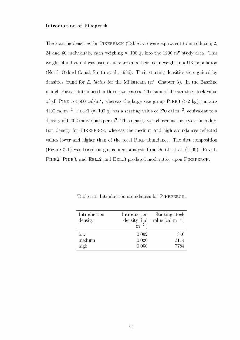
Introduction of Pikeperch

The starting densities for Pikeperch (Table 5.1) were equivalent to introducing 2,

24 and 60 individuals, each weighing ≈ 100 g, into the 1200 m² study area. This

weight of individual was used as it represents their mean weight in a UK population

(North Oxford Canal; Smith et al., 1996). Their starting densities were guided by

densities found for E. lucius for the Millstream (cf. Chapter 3). In the Baseline

model, Pike is introduced in three size classes. The sum of the starting stock value

of all Pike is 5500 cal/m², whereas the large size group Pike3 (>2 kg) contains

4100 cal m−2. Pike1 (≈ 100 g) has a starting value of 270 cal m−2, equivalent to a

density of 0.002 individuals per m². This density was chosen as the lowest introduc-

tion density for Pikeperch, whereas the medium and high abundances reflected

values lower and higher than of the total Pike abundance. The diet composition

(Figure 5.1) was based on gut content analysis from Smith et al. (1996). Pike1,

Pike2, Pike3, and Eel 2 and Eel 3 predated moderately upon Pikeperch.

Table 5.1: Introduction abundances for Pikeperch.

Introductiondensity

Introductiondensity [ind

m−2 ]

Starting stockvalue [cal m−2 ]

low 0.002 346medium 0.020 3114high 0.050 7784

91

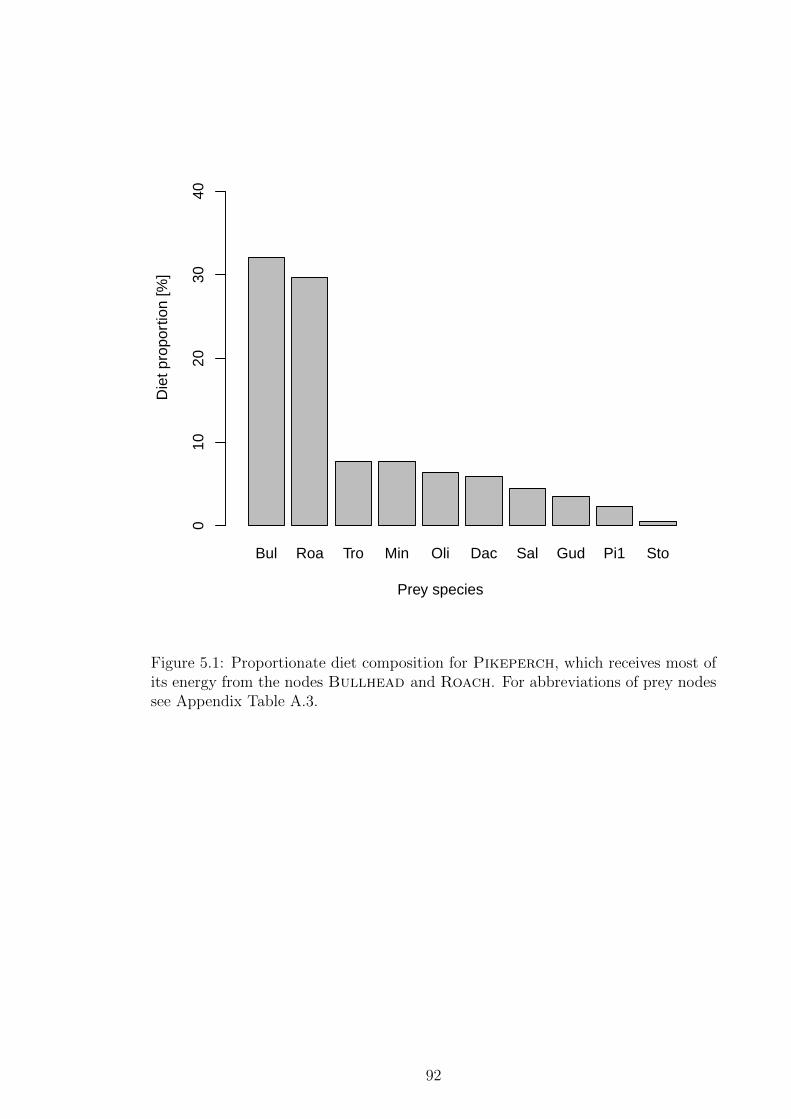
Bul Roa Tro Min Oli Dac Sal Gud Pi1 Sto

Prey species

Die

t pro

port

ion

[%]

010

2030

40

Figure 5.1: Proportionate diet composition for Pikeperch, which receives most ofits energy from the nodes Bullhead and Roach. For abbreviations of prey nodessee Appendix Table A.3.

92

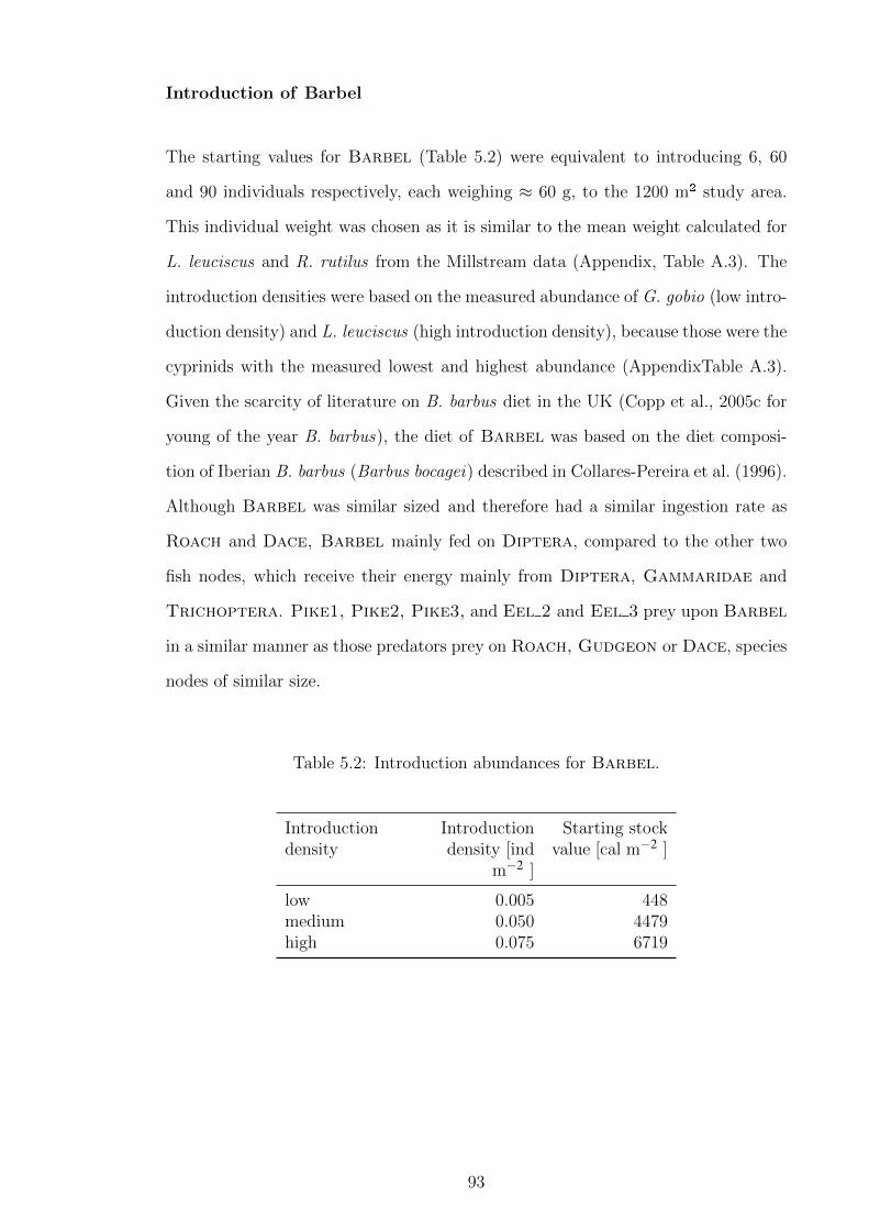
Introduction of Barbel

The starting values for Barbel (Table 5.2) were equivalent to introducing 6, 60

and 90 individuals respectively, each weighing ≈ 60 g, to the 1200 m² study area.

This individual weight was chosen as it is similar to the mean weight calculated for

L. leuciscus and R. rutilus from the Millstream data (Appendix, Table A.3). The

introduction densities were based on the measured abundance of G. gobio (low intro-

duction density) and L. leuciscus (high introduction density), because those were the

cyprinids with the measured lowest and highest abundance (AppendixTable A.3).

Given the scarcity of literature on B. barbus diet in the UK (Copp et al., 2005c for

young of the year B. barbus), the diet of Barbel was based on the diet composi-

tion of Iberian B. barbus (Barbus bocagei) described in Collares-Pereira et al. (1996).

Although Barbel was similar sized and therefore had a similar ingestion rate as

Roach and Dace, Barbel mainly fed on Diptera, compared to the other two

fish nodes, which receive their energy mainly from Diptera, Gammaridae and

Trichoptera. Pike1, Pike2, Pike3, and Eel 2 and Eel 3 prey upon Barbel

in a similar manner as those predators prey on Roach, Gudgeon or Dace, species

nodes of similar size.

Table 5.2: Introduction abundances for Barbel.

Introductiondensity


m−2 ]

Starting stockvalue [cal m−2 ]

low 0.005 448medium 0.050 4479high 0.075 6719

93

Dip Tri Eph Gam Mol Col

Prey species

Die

t pro

port

ion

[%]

020

4060

8010

0

Figure 5.2: Proportionate diet composition for Barbel. Almost all energy is re-ceived from the node Diptera. For abbreviations of prey nodes see AppendixTable A.3.

94

Introduction of TopGud

The starting values for TopGud (Table 5.3) were equivalent to introducing 240, 600,

1200, and 2400 individuals, each weighing ≈ 1 g to the 1200 m2 study area. The

mean weight was chosen based on the assumption that the mean individual would

have a fork-length between 3 cm (approximate size that maturity is reached) and

8 cm (common length, Berg, 1964). The low introduction density chosen was slightly

less than the starting stock values of Gudgeon and then doubled respectively. As

P. parva has been reported to occur in very high densities (Britton et al., 2010c;

Gozlan et al., 2010a), then it is also introduced at an additional, higher density.

In the Baseline Model, Minnow has the highest density with approximately 1 ind.

m−2 (2272 cal m−2). This density is doubled for TopGud (very high density). The

diet composition of TopGud is closely matching the diet composition of Gudgeon,

consisting of Diptera, Gammaridae and Trichoptera. This choice is justified

as although found for a pond community, P. parva and gudgeon do not have signif-

icant differences in their diet (Declerck et al., 2002). The values for body size and

the diet composition has been chosen to simulate a competitor with higher ingestion

rates per gram body weight, with a similar diet composition compared to gudgeon.

For other nodes, Diptera, Gammaridae and Trichoptera also formed an im-

portant part of the diet (e.g. Minnow, Stoneloach, Salmon and Trout), but

in different proportions. Pike1, Pike2, Pike3, and Eel 2 and Eel 3 preyed on

TopGud in a similar manner as Minnow and Bullhead, since those fish were of

similar size as the introduced node.

95

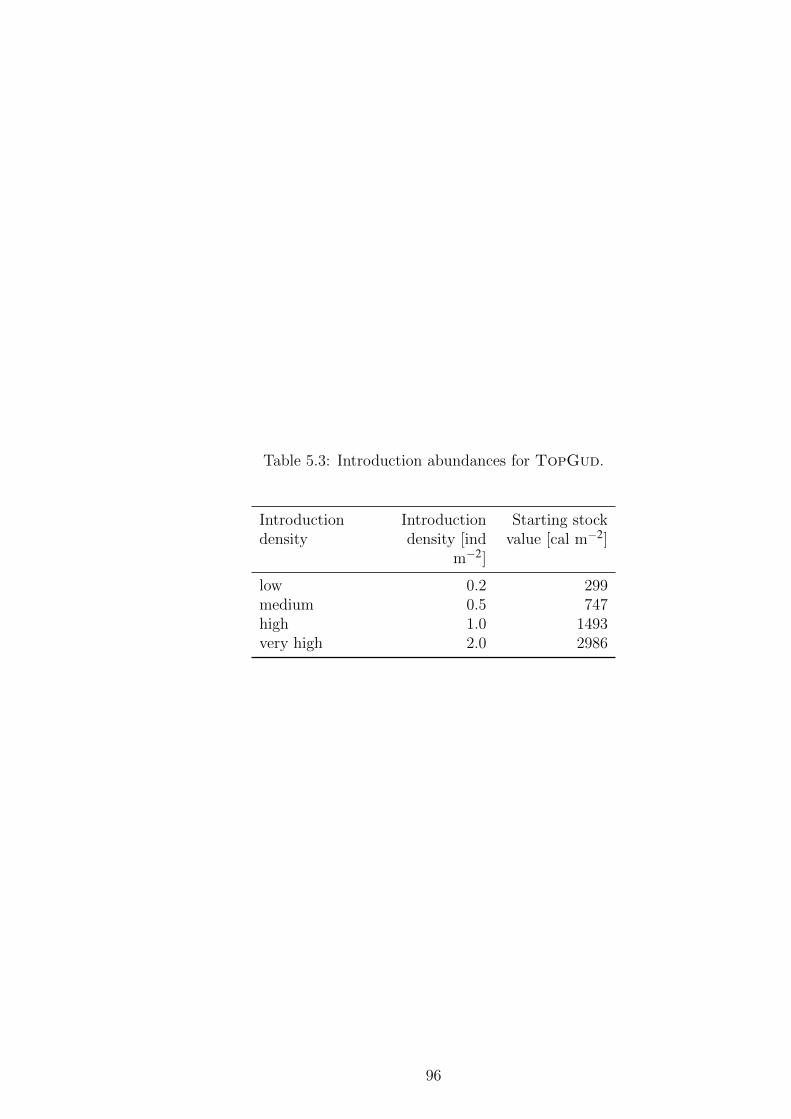
Table 5.3: Introduction abundances for TopGud.

Introductiondensity


m−2]

Starting stockvalue [cal m−2]

low 0.2 299medium 0.5 747high 1.0 1493very high 2.0 2986

96

Gam Dip Tri

Prey species

Die

t pro

port

ion

[%]

010

2030

4050

6070

Figure 5.3: Proportionate diet composition for TopGud. Most of the energy isreceived from the node Gammaridae. For abbreviations of prey nodes see AppendixTable A.3.

97

5.3 Results

Introduction of Pikeperch

In general, the impacts of Pikeperch introduction were stronger with increased

number of introduced individuals. Their introduction caused a decrease in species

diversity, which was calculated for the entire community, including with and with-

out Pikeperch. As introduction density increased, diversity declined (Table 5.4).

Eight of the 14 fish nodes showed a decrease after introduction, with Roach going

extinct at the medium and high introduction density (Figure 5.4). A large increase

(50%) was apparent for Dace. Pikeperch mainly had a negative effect on its prey

nodes, but also on other top predators, namely Eel 2, Eel 3 and Pike2. Although

both Bullhead and Roach form the largest part of the Pikeperch diet (≈ 30%

each), the nodes were affected differently. Bullhead abundance was less affected,

while Roach declined to extinction. The abundance of macroinvertebrate nodes was

hardly affected with the exception of the increased abundance of Ephemeroptera.

In all cases the final stock values of Pikeperch were also substantially lower than

the introduction densities.

Table 5.4: Shannon-Diversity Index (H’ ) for the communities after the introductionof Pikeperch at different densities. The values in brackets are the effective numberof species (true diversity, exp (H’ )).

Community H’ (exp (H’ )) H’ withoutPikeperch

abundance(exp (H’ ))

Pikeperch high 2.43 (11.4) 2.37 (10.7)Pikeperch medium 2.44 (11.5) 2.38 (10.8)Pikeperch low 2.50 (12.2) 2.48 (11.9)Baseline Model 2.54 (12.7)

The community shift, measured by the Bray-Curtis coefficient, revealed that with

rising introduction densities the distance between the Baseline Model and the re-

98

sulting communities became larger (Figure 5.5). The result was not due to the effect

that the addition of a node would have in making the community more dissimilar,

even when the remaining abundances remained the same, since nodes that are not

present in one community are not included in the calculation of the Bray-Curtis

distance measure. Out of the three model species, Pikeperch is the only one that

caused an extinction (Roach, at medium and high density) after introduction.

99

Ppe Bul

Dac

Ee1

Ee2

Ee3

Gud Min

Pi1

Pi2

Pi3

Roa Sal

Sto Tro

LowMediumHigh

Diff

eren

ce in

abu

ndan

ce [%

]

−100

−50

0

50

100

(a)

Col

Dip

Eph

Gam M

ol Oli

Ple Tr

i

LowMediumHigh

Diff

eren

ce in

abu

ndan

ce [%

]

−100

−50

0

50

100

(b)

Figure 5.4: Impact of Pikeperch (Ppe) introduction at different densities on theabundance of fish nodes (a) and macroinvertebrate nodes (b) in relation to the finalvalues of the Baseline model. The values for Pikeperch are in relation to itsrespective starting stock values. For abbreviations see Appendix Table A.3.

100

Figure 5.5: MDS ordination for the resulting communities after Pikeperch intro-duction. The points mark the distance of the communities resulting from differentintroduction densities (low, medium and high) to the Baseline Model. The axis aredimensions. Stress: 0.00%

101

Introduction of Barbel

The introduction of Barbel had little impact on the food web at all introduc-

tion densities. The Shannon Index slightly increased, as would be expected when

a species is added to the community (Table 5.5). No difference was found to the

Shannon Index calculated without Barbel abundance. Barbel introduction had

a positive effect on Pike1 at low introduction density, but negative at medium intro-

duction density (Figure 5.6). Salmon decreased, but the decrease is larger at low

introduction density. The increase in Plecoptera appears very large (Figure 5.6),

but the node had a very low starting abundance (0.7 cal m−2) and only increased

to 1 cal m−2. The final stock values of Barbel were slightly lower than the start-

ing stock values in all three cases. There was no trend towards a community shift

recognisable in the MDS graph (Figure 5.7). The resulting communities all have a

similar distance to the Baseline Model.

Table 5.5: Shannon-Diversity Index (H’ ) for the communities after the introductionof Barbel at different densities. The values in brackets are the effective number ofspecies (true diversity, exp (H’ )).

Community H’ (exp (H’ )) H’ without Barbelabundance(exp (H’ ))

Baseline Model 2.54 (12.7)Barbel high 2.56 (12.9) 2.56 (12.9)Barbel low 2.57 (13.1) 2.57 (13.1)Barbel medium 2.60 (13.5) 2.60 (13.5)

102

Bar Bul

Dac

Ee1

Ee2

Ee3

Gud Min

Pi1

Pi2

Pi3

Roa Sal

Sto Tro

LowMediumHigh

Diff

eren

ce in

abu

ndan

ce [%

]

−100

−50

0

50

100

(a)

Col

Dip

Eph

Gam M

ol Oli

Ple Tr

i

LowMediumHigh

Diff

eren

ce in

abu

ndan

ce [%

]

−100

−50

0

50

100

(b)

Figure 5.6: Impact of Barbel (Bar) introduction at different densities on the abun-dance of fish nodes (a) and macroinvertebrate nodes (b) relative to the final values ofthe Baseline model. The values for Barbel are in relation to its respective startingstock values. For abbreviations see Appendix Table A.3.

103

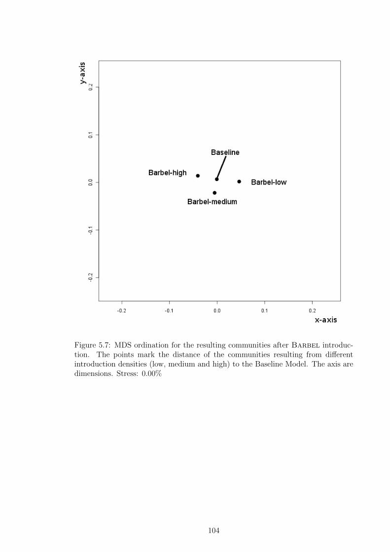
Figure 5.7: MDS ordination for the resulting communities after Barbel introduc-tion. The points mark the distance of the communities resulting from differentintroduction densities (low, medium and high) to the Baseline Model. The axis aredimensions. Stress: 0.00%

104

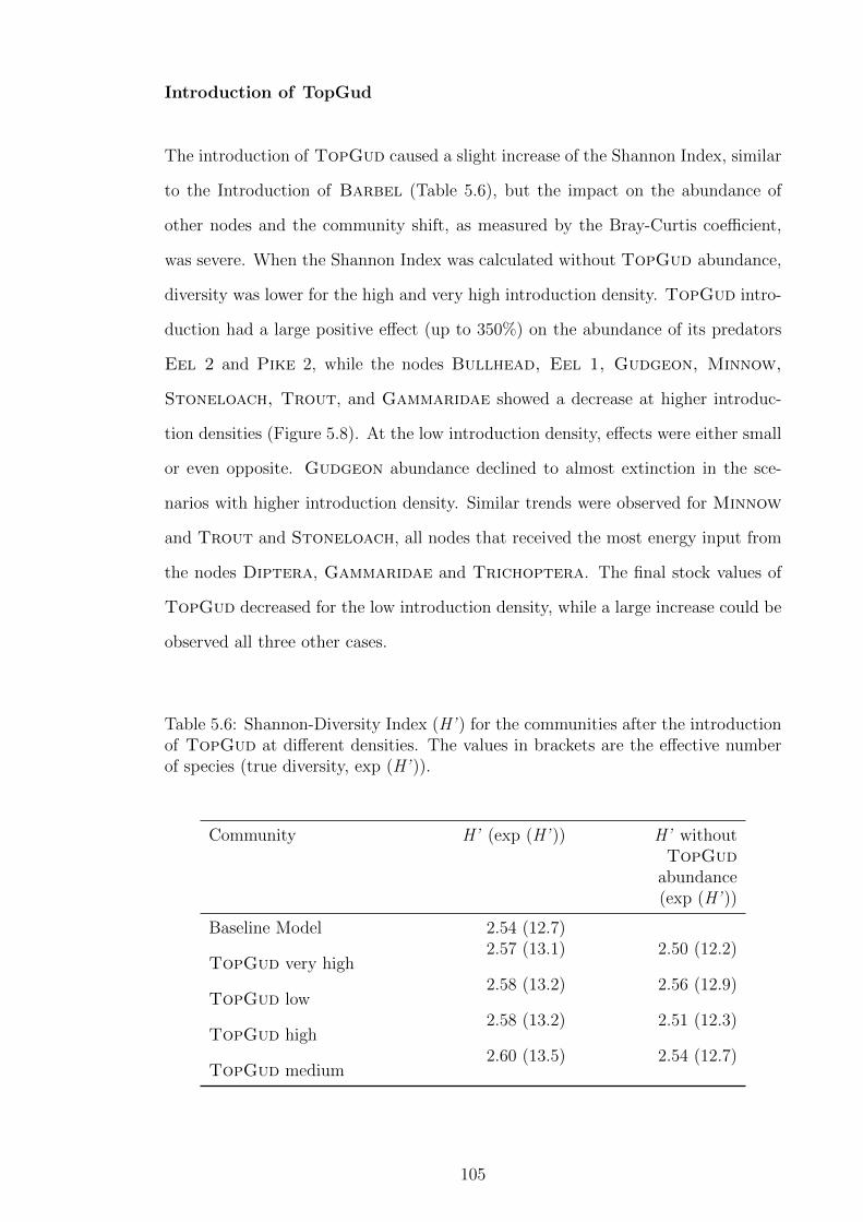
Introduction of TopGud

The introduction of TopGud caused a slight increase of the Shannon Index, similar

to the Introduction of Barbel (Table 5.6), but the impact on the abundance of

other nodes and the community shift, as measured by the Bray-Curtis coefficient,

was severe. When the Shannon Index was calculated without TopGud abundance,

diversity was lower for the high and very high introduction density. TopGud intro-

duction had a large positive effect (up to 350%) on the abundance of its predators

Eel 2 and Pike 2, while the nodes Bullhead, Eel 1, Gudgeon, Minnow,

Stoneloach, Trout, and Gammaridae showed a decrease at higher introduc-

tion densities (Figure 5.8). At the low introduction density, effects were either small

or even opposite. Gudgeon abundance declined to almost extinction in the sce-

narios with higher introduction density. Similar trends were observed for Minnow

and Trout and Stoneloach, all nodes that received the most energy input from

the nodes Diptera, Gammaridae and Trichoptera. The final stock values of

TopGud decreased for the low introduction density, while a large increase could be

observed all three other cases.

Table 5.6: Shannon-Diversity Index (H’ ) for the communities after the introductionof TopGud at different densities. The values in brackets are the effective numberof species (true diversity, exp (H’ )).

Community H’ (exp (H’ )) H’ withoutTopGud

abundance(exp (H’ ))

Baseline Model 2.54 (12.7)

TopGud very high2.57 (13.1) 2.50 (12.2)

TopGud low2.58 (13.2) 2.56 (12.9)

TopGud high2.58 (13.2) 2.51 (12.3)

TopGud medium2.60 (13.5) 2.54 (12.7)

105

The largest shift from the Baseline Model was observed after TopGud introduc-

tion at medium and high densities (Figure 5.9). The MDS graph for TopGud

has a different scale to the MDS graphs for Barbel and Pikeperch introduction

(Figures 5.5 and 5.7). When all communities are compared in one graph, Bar-

bel, Pikeperch and TopGud-low could not be distinguished from the Baseline

Model (Figure 5.10). Although the Shannon Index decreased more after Pikeperch

introduction, this was not captured in the MDS graph.

106

Top

Bul

Dac

Ee1

Ee2

Ee3

Gud Min

Pi1

Pi2

Pi3

Roa Sal

Sto Tro

LowMediumHighVery high

Diff

eren

ce in

abu

ndan

ce [%

]

−100

0

100

200

300

400

(a)

Col

Dip

Eph

Gam M

ol Oli

Ple Tr

i

LowMediumHighVery high

Diff

eren

ce in

abu

ndan

ce [%

]

−100

−50

0

50

100

(b)

Figure 5.8: Impact of TopGud (Top) introduction at different densities on theabundance of fish nodes (a) and macroinvertebrate nodes (b) relative to the finalvalues of the Baseline model. The values for TopGud are in relation to its respectivestarting stock values. For abbreviations see Appendix Table A.3.

107

Figure 5.9: MDS ordination for the resulting communities after TopGud intro-duction. The points mark the distance of the communities resulting from differentintroduction densities (low, medium, high and very high) to the Baseline Model. Theaxis are dimensions. Note the scale of the axes differ to those used for Pikeperchand Barbel. Stress: 0.00%.

108

Figure 5.10: MDS ordination for all resulting communities after introductions. Theaxis are dimensions. On this scale the resulting communities after introductionof Pikeperch and Barbel at all introduction densities fall on one point withthe Baseline Model community. The same applies to TopGud at low density. OnlyTopGud at higher introduction densities are different in comparison. Stress: 0.01%.

109

5.4 Discussion

The introduction of new species nodes into the food web model has different impacts

on community structure depending on the characteristics of the introduced species.

TopGud caused the greatest community shift at higher introduction densities, while

Pikeperch caused the largest decline in diversity. Barbel introduction, however,

did not seem to affect community structure at any introduction density.

The analysis of species introduction on the abundance of single nodes revealed that

Pikeperch elicits strong top-down effects on its main prey. The results also sug-

gested that impacts could not be deduced from the diet composition, since e.g. Dace

became more abundant, although it forms about 10% of Pikeperch’s diet. The

main prey nodes, (Bullhead and Roach, both ≈ 30%) also responded differently

to the introduction. Both nodes decreased, but Bullhead only decreased by ≈ 15%

at the medium and high introduction density, whereas Roach became extinct. The

prediction of the model was consistent with findings that S. lucioperca can elicit

a negative impact on cyprinid fish populations, such as R. rutilus, common carp

(Cyprinus carpio) and common bream (Abramis brama) (Klee, 1981; Linfield, 1982;

Smith et al., 1994, 1996). Notwithstanding, other authors have found no impact on

prey fish populations (Hickley and North, 1983; Adams, 1993) or concluded that a

decline in prey fish biomass cannot be attributed solely to predation by S. lucioperca

(Leah and Kell, 1985). In a subsequent study, Smith et al. (1998) reviewed all S.

lucioperca impact studies and found the evidence of S. lucioperca impacting on prey

populations to be equivocal. The only apparent impact was demonstrated in an ar-

tificial environment in which an upstream and downstream section of adjacent canal

stretches was compared, rather than comparing the same stretch before and after

the introduction. Differences in cyprinid fish densities could therefore be explained

by other, unexplored factors (Smith et al., 1998). Consequently, the model predic-

tions contradict those findings at least at the higher introduction densities. Given

the model excluded the role of environmental factors in determining impacts, then it

demonstrated that the introduction of Pikeperch (or indeed other top predators)

110

have the potential to reduce prey fish abundance and diversity within a food web

context. Pikeperch introduction also caused a decline in the other top predators,

except Pike3. The increases in Dace, Salmon and Stoneloach could either

be due to less predator pressure from Eel and Pike, or less competition from the

other fish nodes, which decreased in abundance, or a combination of both. There

is, however, no evidence for a system shift after the introduction of Pikeperch

as measured by the Bray-Curtis distance, but the largest decrease in the Shannon

Index was observed.

In a comparative study of 12 different river basins in South Korea after the intro-

duction of the piscivorous largemouth bass (Micropterus salmoides), similar results

to the model predictions have been found (Jang et al., 2006). M. salmoides pop-

ulated sites had significantly lower abundance of other piscivorous predators. Four

of six prey fish were also significantly less abundant, while two were significantly

more abundant. Not all observed effects could be solely assigned to the presence

of M. salmoides, since its distribution also correlates with environmental factors.

Although M. salmoides exhibited a higher degree of piscivory in the South Korean

study than in similar studies in North America, Europe and Africa, it preyed mostly

on the most common prey species and was not considered a major threat to less

abundant, endemic species (Jang et al., 2006). Possible diet shifts that accompany

prey species abundance patterns could therefore be specific to the ecosystem to

which a top predator is introduced. In regard to the interaction of S. lucioperca

with other top predators, such as E. lucius, environmental factors, such as increased

turbidity, which favours S. lucioperca (G.H. Copp, pers. com.), may pose additional

influences on community composition.

A further example is the intentional introduction of piscivorous peacock bass (Ci-

chla kelberi) into the Rosana Reservoir (Parana River basin, Brasil; Pelicice and

Agostinho, 2009). After the introduction of C. kelberi, species diversity decreased

severely, and after a few years, a nearly complete loss of fish assemblages was noted.

The loss of prey species was described as non-linear, as large losses in biodiversity

and prey abundance coincided with large shoals of young C. kelberi during summer,

111

whereas fish assemblages recovered during spring, when juvenile C. kelberi were ab-

sent (Pelicice and Agostinho, 2009). Potentially, juvenile S. lucioperca could exert

similar predation pressure when introduced into the Frome catchment, adding to

the impacts predicted by the food web model.

Although the starting value of TopGud (measured in cal m−2) was lower at the

highest introduction density than medium introduction densities for Barbel and

Pikeperch, TopGud introduction had the largest impact at higher introduction

densities according to MDS analysis. In response to the introduction of TopGud,

nodes with similar diet composition decreased, while some of the top predator nodes

increased (Eel 2, Eel 3, and Pike2 showed particularly large increase). Gud-

geon abundance declined to almost extinction in the scenarios with higher intro-

duction density, which could be due to competition, increased predator pressure, or

to a combination of both. Similar trends were observed for Minnow and Trout

and Stoneloach, all nodes that received the most energy input from the nodes

Diptera, Gammaridae and Trichoptera. Since Gammaridae decreased, at

least some of the decrease in the fish nodes could be assigned to competition. Those

findings are also consistent with the assumption that P. parva is a strong competitor

for food resources (Witkowski, 2006; Britton et al., 2010c; Gozlan et al., 2010a). P.

parva might be the better competitor for energy because of its size, as small indi-

viduals have a higher ingestion rate per gram body weight (Peters, 1983) and the

flow rates between the nodes are based on the ingestion rate.

The increase in the predators of TopGud also suggested a bottom-up effect. In

return, increased top predator body mass could have top-down effects on their prey

nodes. The addition of the top predator, Pikeperch, also caused a decrease in

Gudgeon and Trout, so some of the decrease could be explained by increased

top-down effects. Roach was strongly affected by the introduction of Pikeperch,

going extinct at the higher introduction densities. Contrary, Roach abundance

increased after TopGud introduction. Roach only forms a small part of the Pike

diet and Eel did not prey on Roach at all. This might be the reason why Roach

is unaffected by the increased abundance after TopGud introduction. Pikeperch

112

received 30% of its energy demand from Roach, resulting in a strong top-down

control.

In a comparative study of two ponds with similar community composition of which

one was invaded by P. parva, no changes in composition or abundance of the fish

community were found, although P. parva was the numerically dominant fish in the

invaded pond (60 m−2; Britton et al., 2010c). Even the highest introduction density

for TopGud into the food web model was distinctively lower (2 m−2). The present

study found a high impact on community composition, which could be explained by

the different nature of the habitat (lotic vs. lentic) and fish community composition

(Britton et al., 2010c). The ponds were inhabited by five native fish species and top

predators were absent. Although a shift in the trophic position of rudd (Scardinius

erythropthalmus) suggested that it preyed on P. parva in the invaded pond, this

suggestion would not be supported by gut content analysis. However, P. parva

was found to depress somatic growth in R. rutilus, a finding that contradicts the

predicted higher abundance of Roach in the food web model, although abundance is

measured in cal m−2 rather than individual growth. When interpreting the different

results, it has to be kept in mind that the implementation of TopGud diet into

the model was intentionally chosen to display high competition with Gudgeon.

Contrary to the findings of Britton et al. (2010c), TopGud can be assumed to have

impacted on other species nodes through competition and also through bottom-up

effects on top predators, which in turn elicited top-down effects. In the model,

Roach was hardly affected by those top-down effects and its abundance increased.

Therefore, the impacts that a small, highly abundant, competitive species might have

on a system with and without top predators is likely to be substantially different.

The introduction of Barbel had no notable impact on the abundance of other

nodes. The food web seemed to be resilient to the addition. Barbel received its

energy input mainly from Diptera, with small inputs from other macroinverte-

brate nodes. Compared to the diet composition of TopGud, Barbel was a more

specialised forager and occupied a different niche, which resulted in no detectable

competition for energy with the other nodes. The ingestion rate for the larger-bodied

113

Barbel was also lower per gram body weight. Although B. barbus had been intro-

duced to western and southern England and parts of Italy, negative impacts that are

specific to their introduction have not been reported (Bianco and Ketmaier, 2001).

The low impact Barbel introduction had on community composition, combined

with the absence of reported ecological impacts, suggested that B. barbus introduc-

tions to chalk streams to enhance the recreational fishery may not result in adverse

impacts on stream community structure.

The establishment of the three introduced species nodes followed a different pattern.

Pikeperch abundance was in all three cases lower (41=90%) after the model re-

laxed into the final stable state than introduction abundance, suggesting that only

a certain number of individuals could be supported. For TopGud the trend was

reversed. Except for the low introduction density, where abundance decreased by

≈ 60%, an increase in abundance (30=60%) could be observed. There seemed to be

a critical abundance, at which TopGud was able to either out-compete other nodes

with a similar diet, or started to have bottom-up effects on top predator nodes. The

change in abundance of the nodes after TopGud introduction suggested a combina-

tion of both (Figure 5.8). At the low introduction density, TopGud had a positive

effect on the abundance of Gudgeon, Bullhead and Stoneloach, while Pike2

abundance decreased. The final stock value of Barbel was in all three cases ≈ 10%

less than the introduction density, suggesting that although no major impacts could

be detected on community composition, a consistent abundance of Barbel was

supported.

From the three model species added to the food web, two elicited changes in the

abundance of other nodes and biodiversity: the top predator and the strong com-

petitor. Further investigation is required to ascertain whether the impact caused

by TopGud introduction is due to the diet overlap or the high ingestion rate per

gram body weight. Presently, the literature is scarce of evidence that ingestion or

metabolic rate per gram body weight could be a predicting factor of the invasiveness

of a species, although it has been suggested that metabolic rate, which scales with

body mass, could be used to predict how the individual affects the dynamics and

114

structure of populations, communities and ecosystems (metabolic theory of ecology;

Brown et al., 2004). Concepts of the metabolic theory of ecology have been applied to

ecological networks to estimate interaction strengths between consumers and their

resources (Emmerson and Woodward, 2005; Woodward et al., 2005a; Otto et al.,

2007; Yvon-Durocher et al., 2008). Stocking up top-predators into the ecosystem

can either result in decline of native top-predators because the introduced species

replaces them, or increase in predator species richness (Eby et al., 2006). In the

present case, Pikeperch introduction caused the other top predators to decline,

which corroborates observations in waters characterised by elevated turbidity but is

contrary to low turbidity waters, where native E. lucius is normally the predomi-

nant of the two top predators (G.H. Copp, pers. comm.). The energy flow model

also shows that it is difficult to predict how the abundance of nodes will be affected,

since bottom-up and top-down effects have been seen simultaneously. This has im-

plications for biomanipulation, especially for species rich ecosystems. Direct effects

can also be mitigated through indirect effects. For example, although Pikeperch

preys directly on Salmon, Dace and Stoneloach, the abundance of those three

nodes was affected positively after Pikeperch introduction.

In real food webs, individuals can change their behaviour (McIntosh and Townsend,

1995), shift their diet (Declerck et al., 2002; Baxter et al., 2004), or be favoured

by environmental factors, such as discharge regimes (Marchetti and Moyle, 2001;

Thomson et al., 2002; Franssen et al., 2007). Predator impacts on food web struc-

ture can also depend on habitat type (Nystrom et al., 2003) and disturbance history

(Nystrom and McIntosh, 2003). Further impacts could be caused by habitat mod-

ification (e.g. Miller and Crowl, 2006), disease transmission (Blanc, 1997; Gozlan

et al., 2005; Gozlan, 2008b), or hybridisation (Gozlan et al., 2010b). The impacts

detected by the food web model might be mitigated or amplified by these factors.

P. parva, for example, has been shown to interfere with the reproduction of native

species (Britton et al., 2007) and is also a healthy carrier of the rosette agent S.

destruens (Gozlan et al., 2005). The food web model does not contain egg or larval

species, so P. parva could have non-trophic impacts on the abundance of other fish

115

by being a healthy carrier of a pathogen and additional trophic impacts by preying

on larval stages and eggs of fish. Impacts of diet shifts in native species after an

introduction have been shown to not only impact on the aquatic system, but also

on the surrounding terrestrial community. The introduction of rainbow trout (On-

corhynchus mykiss), which mainly feeds on terrestrial prey that falls into streams,

to rivers in northern Japan caused native Dolly Varden charr (Salvelinus malma)

to shift their diet from terrestrial prey to aquatic insects that graze algae (Baxter

et al., 2004). This also decreased the abundance of riparian spiders that specialise on

emerging adult aquatic insects (Baxter et al., 2004). Changes in stream discharge,

or in a wider sense habitat modification caused by water abstraction, favoured non-

native species in a Californian regulated stream (Marchetti and Moyle, 2001). The

abundance of native species on the other hand, was positively affected by a natural

discharge regime, which is defined by higher discharge. These examples illustrate

the importance of considering environmental factors and behavioural changes when

applying the results from the energy flow model to conservation decisions.

The model was specifically developed for an energy- and species-rich chalk stream.

The impacts of introductions in other lotic systems might be different and should,

therefore, be tested. Negative and positive effects have also been reported for the

same species (Leprieur et al., 2009), which shows that the impact of species might

be context dependent. The detected impacts on community structure in the present

study are purely explainable by trophic interactions. Although species abundance

was influenced by introductions, and a large shift was observed after TopGud intro-

duction, a collapse of the food web was not observed in any of the trials. Additional

stressors, such as habitat degradation and environmental change, may therefore play

a major role when extinctions are observed (Gurevitch and Padilla, 2004). Future

research is needed to determine whether or not the large shift caused by TopGud

introduction was caused by the high diet overlap, by the higher ingestion rate due to

its smaller body size, or by the combination of both. Although the diet of Barbel

was not implemented to simulate competition, it still received its energy from the

main prey nodes, but did not elicit detectable changes. Therefore, it is concluded

116

that ingestion rates could play a major role in determining the impact an introduced

species can have on food web structure.

117

Chapter 6

Impact of rising temperatures on

energy flows and distribution

within an aquatic food web.

6.1 Introduction

Climate change currently constitutes one of the key global ecological impacts as

evidence suggests that the warming process is presently going faster than in the past

1000 years (IPCC, 2007). Climate has always varied temperatures during the earth’s

history, and this has had a profound influence on the distribution of organisms.

Notwithstanding, the current rate at which the environment will change is expected

to be too fast for ecosystems to adapt (Mulholland et al., 1997; Malmqvist and

Rundle, 2002; Folke et al., 2004; Johnson et al., 2009a; Perkins et al., 2010). The

abiotic factors that will directly or indirectly affect aquatic organisms are i) water

temperature (FSBI, 2007; Johnson et al., 2009a), ii) changes in hydrology (indirectly

through change in precipitation; Poff et al., 1997; Fruget et al., 2001; Johnson et al.,

2009a), and iii) CO2 concentrations (through changes in leaf litter composition; Rier

et al., 2002).

During the 20th century, the global mean temperature has risen by 0.6°C, and the

118

projected increase for the next century ranges from 1.4°C to 5.8°C. Physical vari-

ables that are temperature dependent include surface tension, density and viscosity,

organic and non-organic chemical reaction rates and solubility of oxygen and other

gases (Webb, 1996). Temperature has a large effect on aquatic biotas, which are

mostly poikilotherms, as it governs biological processes such as species’ distribution

(Poff et al., 2002; Sims et al., 2004), and metabolism (Fry, 1971; Coutant, 1987;

Regier et al., 1990; Clarke, 1993), with knock-on effects on growth, reproduction,

immune responses to diseases (Le Morvan et al., 1998) and ultimately organism

behaviour (Kramer et al., 1997; Sims et al., 2006).

This combination of physical and biological changes will determine the extent of

shifts in the geographical distribution of organisms. Since enzymatic rates are tem-

perature dependent, and the body temperature of poikilotherms varies according to

the surrounding water temperature, fish metabolism is directly linked to water tem-

perature, with direct consequences on food consumption and growth (Brander, 1995;

van Dijk et al., 2002), but also foraging behaviourchanges with temperature (Pers-

son, 1986). An increase in thermophilic species in higher latitudes and altitudes has

already been observed (Daufresne et al., 2004) and fishes are expected to respond to

environmental change by migrating, which might be limited by catchment barriers,

to habitats that continue to provide optimum conditions for their metabolism and,

ultimately, fitness (Allan et al., 2005). Warmer winters and milder springs favour

the recruitment of many cyprinid fishes (Johnson et al., 2009a), whereas cold water

species may experience a reduction in habitat (Mulholland et al., 1997). Indeed,

a temperature rise is predicted to result in a general increase in system productiv-

ity (Benke, 1993; Mulholland et al., 1997). The effects of temperature on different

aspects of fish biology can be summarised categorically (Figure 6.1, 6.2) on the

complicated, interdependent relationships between mortality and growth, which can

respond differently at distinct life-stages, e.g. temperatures that are beneficial for

spawning in adult fish can have fatal consequences on egg development (Sandstrom

et al., 1997). Behavioural responses to compensate for effects make predictions more

difficult. For example, in starving R. rutilus, colder waters are preferred in order to

119

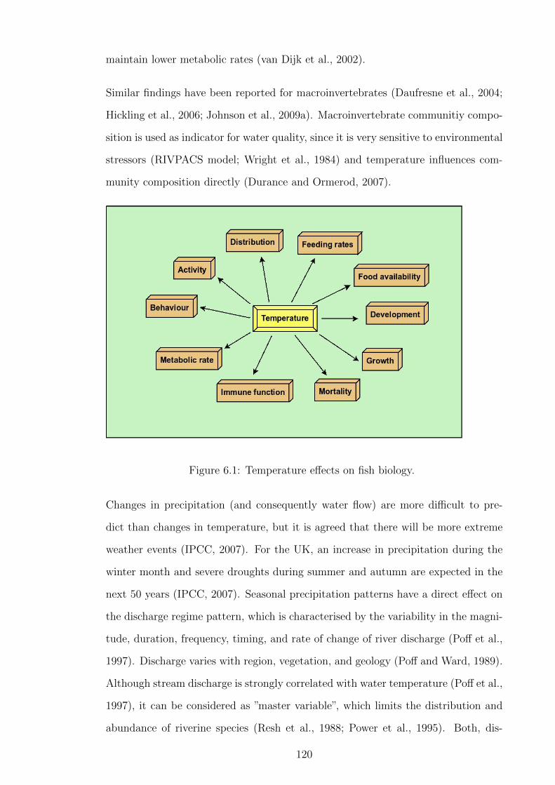
maintain lower metabolic rates (van Dijk et al., 2002).

Similar findings have been reported for macroinvertebrates (Daufresne et al., 2004;

Hickling et al., 2006; Johnson et al., 2009a). Macroinvertebrate communitiy compo-

sition is used as indicator for water quality, since it is very sensitive to environmental

stressors (RIVPACS model; Wright et al., 1984) and temperature influences com-

munity composition directly (Durance and Ormerod, 2007).

Figure 6.1: Temperature effects on fish biology.

Changes in precipitation (and consequently water flow) are more difficult to pre-

dict than changes in temperature, but it is agreed that there will be more extreme

weather events (IPCC, 2007). For the UK, an increase in precipitation during the

winter month and severe droughts during summer and autumn are expected in the

next 50 years (IPCC, 2007). Seasonal precipitation patterns have a direct effect on

the discharge regime pattern, which is characterised by the variability in the magni-

tude, duration, frequency, timing, and rate of change of river discharge (Poff et al.,

1997). Discharge varies with region, vegetation, and geology (Poff and Ward, 1989).

Although stream discharge is strongly correlated with water temperature (Poff et al.,

1997), it can be considered as ”master variable”, which limits the distribution and

abundance of riverine species (Resh et al., 1988; Power et al., 1995). Both, dis-

120

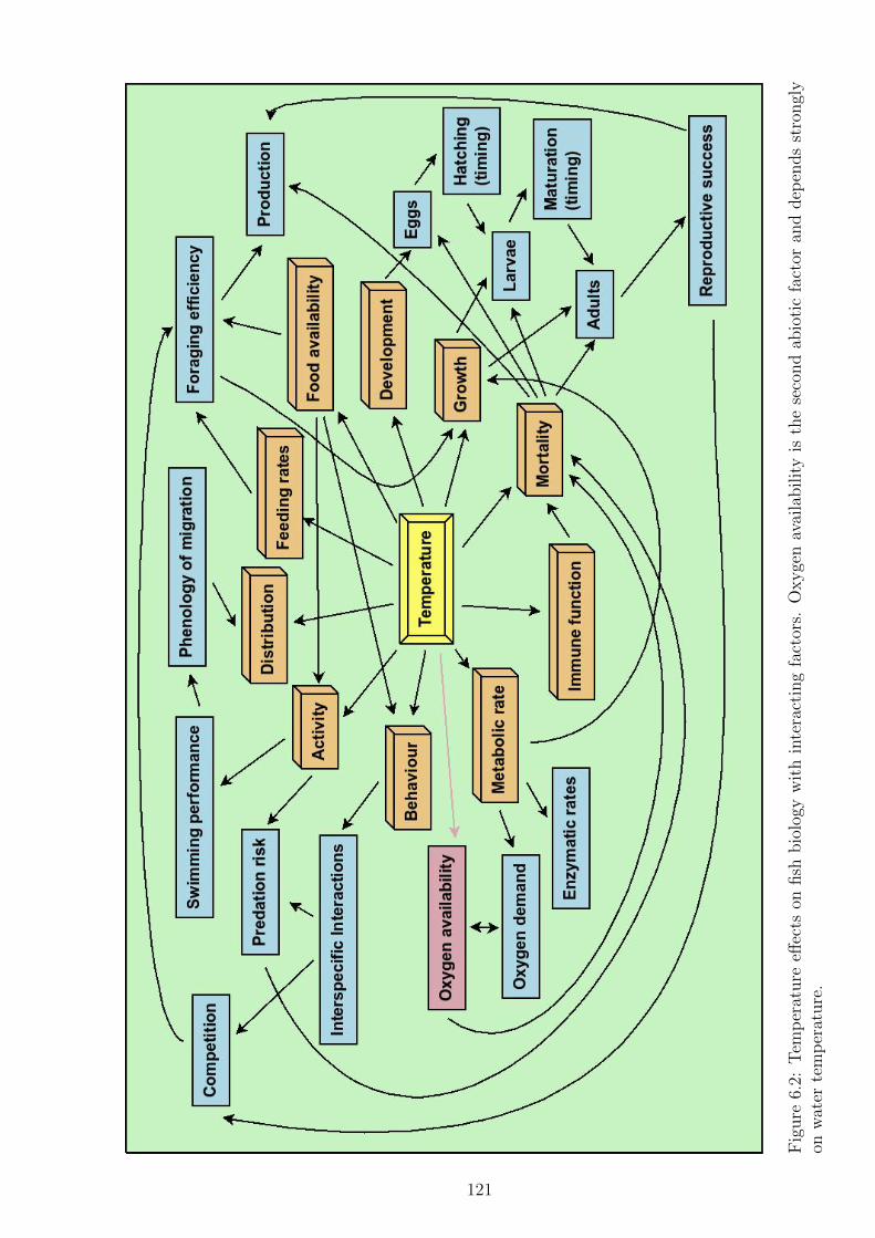
Fig

ure

6.2:

Tem

per

ature

effec

tson

fish

bio

logy

wit

hin

tera

ctin

gfa

ctor

s.O

xyge

nav

aila

bilit

yis

the

seco

nd

abio

tic

fact

oran

ddep

ends

stro

ngl

yon

wat

erte

mp

erat

ure

.

121

charge and water temperature have been shown to govern long term dynamics of

invertebrate and fish communities (Fruget et al., 2001). The frequency and timing

of precipitation seems to be of particular importance. Variable discharge generally

maintains high levels of biodiversity (Poff et al., 1997), but changes to the natural

discharge regime have been shown to affect biodiversity of fish and certain macroin-

vertebrates adversely, because habitat diversity declines (Poff and Ward, 1989; Mann

and Bass, 1997; Sheldon and Walker, 1997; Baron et al., 2002; Dewson et al., 2007),

in particular, a relationship between low discharge and decreases in biodiversity has

been demonstrated (Xenopoulos et al., 2005). Additionally, the likelihood of fish be-

ing infected by pathogens increases in warm, lentic waters (Johnson et al., 2009a).

Some macroinvertebrate families are favoured by drought conditions and and have

been found to occur in high densities during periods of low discharge (Dewson et al.,

2007). Macroinvertebrate communities have been shown to recover quickly from

severe droughts without prolonged impact on species richness (Wright and Symes,

1999). There are still gaps in knowledge on how low discharge affects macroinverte-

brate communities, but a shift in community composition towards drought resistant

species, at least during low discharge periods, is certain.

The different scenarios of future carbon dioxide release used in climate change fore-

casts reflect the uncertainty associated with climate change predictions, but global

atmospheric carbon dioxide levels are expected to double within the next 50 years

(Rier et al., 2002). Elevated carbon dioxide can affect leaf chemistry of C3 plants

through increased C fixation and lead to a proportional decrease in N. Increased C

fixation results in less edible detritus input into the river food web, and consequently

slower decompostation of terrestrial leaf litter by microbes. In particular, detritus

based food webs are expected to be affected where lower availability of C and N

at the base of the food web could ultimately decrease production at higher trophic

levels (i.e. macroinvertebrates and fish Rier et al., 2002) and change the distribution

of feeding links (Hall et al., 2000).

The impacts that climate change might have on ecosystems are correspondingly

complex and could affect the physiological and behavioural aspects discussed above.

122

In Chapter 3, the impact of extinctions, e.g caused by raised temperatures or altered

discharge regime, on food web structure was examined. Loss of biodiversity caused

by extinctions and range shifts have been predicted (Poff and Ward, 1989; Mann

and Bass, 1997; Sheldon and Walker, 1997; Baron et al., 2002) and, in some cases,

confirmed (Daufresne et al., 2004; Hickling et al., 2006; Johnson et al., 2009a), but

the impact of elevated temperatures on energy flow and distribution has not been

investigated. In the previous chapters, the assumption was made that the model

system is not energy restricted. Here, the effects of energy restrictions, combined

with elevated metabolic rates, on food web structure, which could lead to a decline in

production and diversity, are investigated. In an ecosystem where the additional en-

ergy demand arising from higher metabolic rates is covered by unrestricted nutrient

supply, production should increase.

Aims and objectives

This chapter aims to identify the impact of increased metabolic rates as response to

elevated temperatures on biodiversity and community composition. The objectives

are:

1. To investigate the influence of elevated metabolic rates without increased en-

ergy input on biodiversity and community composition.

2. To determine the effects of elevated metabolic rates with simultaneously in-

creasing additional energy input on biodiversity and community composition.

123

6.2 Materials and Methods

The energy flow rates of the Baseline Model (Chapter 3) are based on ingestion

rates for poikilotherms. The ingestion rates are gradually increased and the new

flow rates are calculated. Data from experiments using poikilotherms suggest an

increase of between 1.5 and 3.0 times the basic metabolic rate when temperatures

increase by 5°C (Peters, 1983). For the modelling trials, the assumption is made

that the ingestion rates will increase in the same manner. For each increase, the

model is run twice. (1) without an increase in energy input (Community IDs 1–4:

see Table 6.1) to simulate energy restriction, and (2) with an additional energy

input from the environment (Community IDs 5–8) matching the increased ingestion

rates (Table 6.1). The resulting communities are compared in terms of changes in

biodiversity (Shannon index), the extent of extinctions, changes in total energy and

distance between the communities (Bray-Curtis measure). In this context, a species

is considered as extinct if its abundance decreases below 5% of its abundance in the

Baseline Model.

124

Table 6.1: Increase in ingestion rates, which equivalents an increase in temperatureby 5°C, and additional energy input of each trial.

Community ID Increase iningestion rate

Increase inadditional

energy input

1 1.5Ö none

2 2.0Ö none

3 2.5Ö none

4 3.0Ö none

5 1.5Ö 1.5Ö

6 2.0Ö 2.0Ö

7 2.5Ö 2.5Ö

8 3.0Ö 3.0Ö

125

6.3 Results

The communities that received an increased additional energy input (IDs 5–8)

showed no change in species diversity, whereas nutrient-restricted communities showed

a decrease in species diversity (Table 6.2). In the restricted communities, almost all

species nodes became less abundant with increasing metabolic rates. The abun-

dance of nodes, such as Gudgeon, Pike2, Pike3, Roach, Salmon and Trout

decreased over 75% compared to the Baseline Model (Figure 6.3), with an increase

of Coleoptera and Plecoptera. However, both nodes had very low abundances

in the Baseline Model, so that the absolute abundance values hardly changed. Ex-

tinctions occurred in six cases within the energy restricted communities. In Com-

munity 2, Roach went extinct, in community 3, Roach and Pike2, and in Com-

munity 4, Roach, Pike2 and Pike3. In communities that received additional

energy input, no extinctions occurred and abundances hardly changed (Figure 6.4).

MDS analysis supports the findings that the energy restricted communities were

more dissimilar to the Baseline Model (Figure 6.5). With increasing ingestion rates,

communities 1–4 shifted further away, whereas communities 5–8 remained close to

the Baseline Model. The total energy of the system was reduced by 40 to 74% of the

energy stored in the Baseline Model in the energy restricted communities, whereas

only a small positive increase in total energy could be observed when energy was not

restricted (Table 6.3). Fish abundance in communities 1–4 decrease proportionally

more than macroinvertebrate abundance.

126

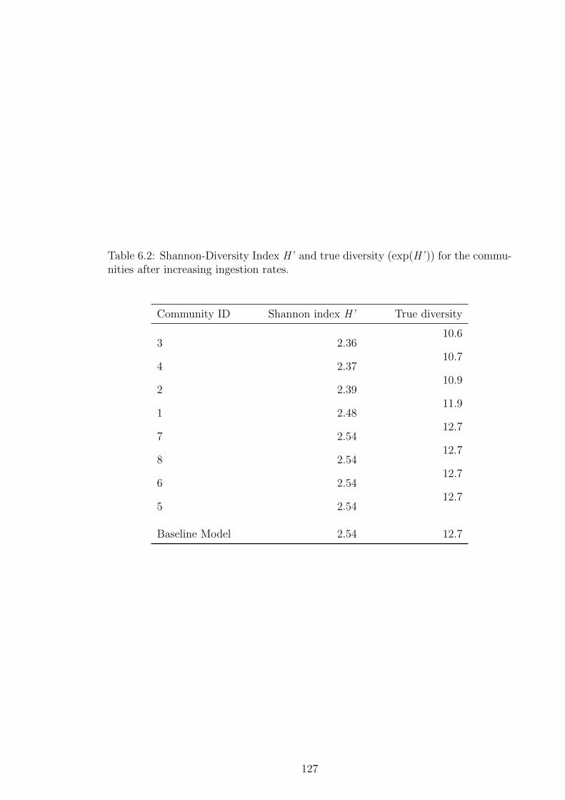
Table 6.2: Shannon-Diversity Index H’ and true diversity (exp(H’ )) for the commu-nities after increasing ingestion rates.

Community ID Shannon index H’ True diversity

3 2.3610.6

4 2.3710.7

2 2.3910.9

1 2.4811.9

7 2.5412.7

8 2.5412.7

6 2.5412.7

5 2.5412.7

Baseline Model 2.54 12.7

127

Col

Dip

Eph

Gam M

ol Oli

Ple Tr

i

Diff

eren

ce in

abu

ndan

ce [%

]

−100

−50

0

50

100

(a)

Bul

Dac

Ee1

Ee2

Ee3

Gud Min

Pi1

Pi2

Pi3

Roa Sal

Sto Tro

ID 1ID 2ID 3ID 4

Diff

eren

ce in

abu

ndan

ce [%

]

−100

−50

0

50

100

(b)

Figure 6.3: Impact of increased ingestion rates with unchanged energy input on theabundance of macroinvertebrate nodes (a) and fish nodes (b) relative to the finalvalues of the Baseline model. For abbreviations see Appendix Table A.3.

128

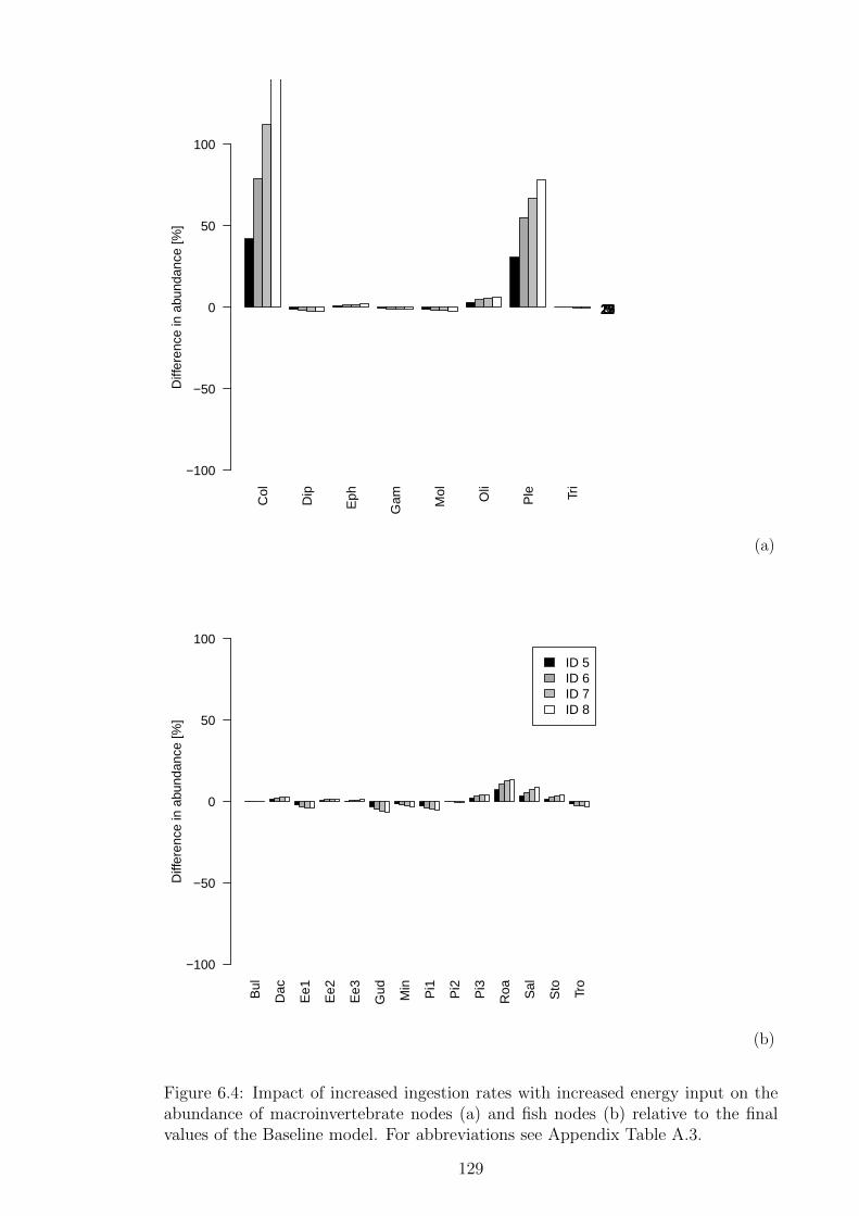
Col

Dip

Eph

Gam M

ol Oli

Ple Tr

i

Diff

eren

ce in

abu

ndan

ce [%

]

−100

−50

0

50

100

1591317212529

(a)

Bul

Dac

Ee1

Ee2

Ee3

Gud Min

Pi1

Pi2

Pi3

Roa Sal

Sto Tro

ID 5ID 6ID 7ID 8

Diff

eren

ce in

abu

ndan

ce [%

]

−100

−50

0

50

100

(b)

Figure 6.4: Impact of increased ingestion rates with increased energy input on theabundance of macroinvertebrate nodes (a) and fish nodes (b) relative to the finalvalues of the Baseline model. For abbreviations see Appendix Table A.3.

129

Figure 6.5: MDS ordination for the communities after increasing the ingestion rates.The axis are dimensions. Stress: 0.00%.

130

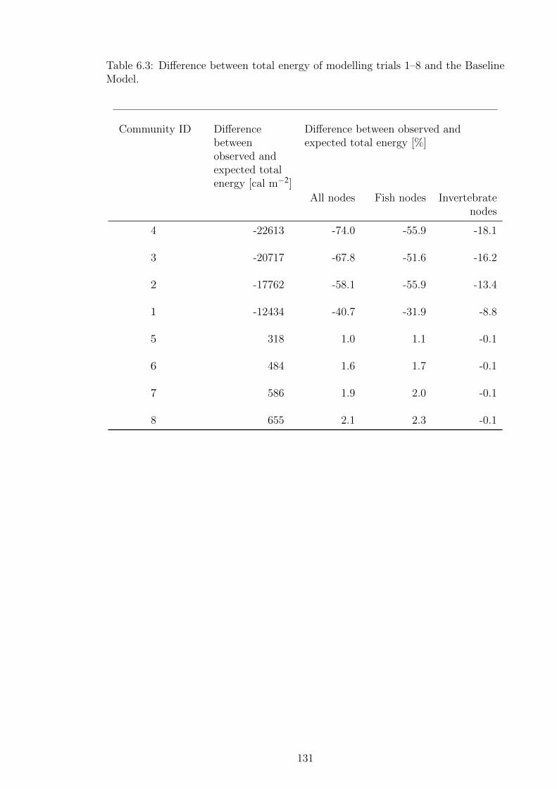
Table 6.3: Difference between total energy of modelling trials 1–8 and the BaselineModel.

Community ID Differencebetweenobserved andexpected totalenergy [cal m−2]

Difference between observed andexpected total energy [%]

All nodes Fish nodes Invertebratenodes

4 -22613 -74.0 -55.9 -18.1

3 -20717 -67.8 -51.6 -16.2

2 -17762 -58.1 -55.9 -13.4

1 -12434 -40.7 -31.9 -8.8

5 318 1.0 1.1 -0.1

6 484 1.6 1.7 -0.1

7 586 1.9 2.0 -0.1

8 655 2.1 2.3 -0.1

131

6.4 Discussion

The effects of climate change are likely to influence numerous aspects of fish phys-

iology or ecology. This chapter investigated the impact of elevated ingestion rates

as a result of increased temperatures on food web structure. The impact of elevated

ingestion rates were catastrophic when energy input into the food web was not raised

to match the higher energy consumption. An overall decrease in species abundance,

biodiversity and total energy was subsequently observed. When the higher energy

expenditure was matched with higher energy inputs, biodiversity and community

composition remained similar to the Baseline Model, with slightly increased values

for total energy (production).

The Millstream food web is strongly dependent on detritus as a baseline energy

source (Westlake et al., 1972; Dawson, 1976; Hynes, 1983); although primary pro-

duction is high, living macrophytes are considered to play a small role as energy

sources for secondary production, since few macroinvertebrates feed on them (New-

man, 1991; Pinder, 1992). Reduced decomposition rates caused by changed nutrient

composition of detritus, as a consequence of increased atmospheric CO2 concentra-

tion, might pose a restriction on energy input at the base of the food web (Rier

et al., 2002). The response of the model system to increased metabolic rates in the

two scenarios highlights the importance of sufficient energy supply. This is only one

aspect of possible responses to climate change, as organisms can show behavioural

adaptions to counteract the found effects, or species might be replaced by species

that belong to the same functional group, but have distinct temperature require-

ments or are better adapted to the changes in leaf litter composition. For example,

Hall et al. (2000) demonstrated that link distributions and intensities changed in

a leaf litter limitated stream and wood became a more important resource. Addi-

tionally, food chain length might decrease with lower energy inputs from detritus

(Jenkins et al., 1992).

Behavioural responses that have been shown for fish include migration and changed

activity patterns, and they could counteract the impact of elevated temperatures

132

by saving energy expenditure. For example, starved R. rutilus showed a preference

for colder waters during night while resting and was less active than R. rutilus held

under control conditions (van Dijk et al., 2002). When sufficient food is available,

warmer temperatures can have positive effects on growth (Garner et al., 1998). P.

phoxinus forage in the main channel of the River Frome, where food is abundant,

but prefer to rest in warmer shallow habitats (although low food availability; Garner

et al., 1998). P. phoxinus in these warmer habitats showed higher growth rates than

fish that remained in the slightly colder main channel. Dependent on food availabil-

ity, these two cyprinid species showed different strategies to maximise growth. In

brook trout (Salvelinus fontinalis), higher growth rates were associated with higher

temperatures in winter and spring, but lower temperatures in summer and autumn

(Xu et al., 2010).

Prolonged warm temperatures in combination with drought conditions might reduce

retreat areas that offer lower temperatures and fish density in those refugia might

increase. Fish retreat both upstream and downstream into refugia during times of

drought and fish assemblages change accordingly (Davey and Kelly, 2007). Migration

and increased mortality due to temperature rise could act as an additional stressors,

with further negative impacts on biodiversity. As demonstrated in Chapter 4, loss

of single species did not have catastrophic consequences on the stability and species

composition of the food web, but migration would create, at least temporally, new

assemblages that potentially have different properties than the studied food web. In

the extreme case of a drought, fish might be confined to pools, in which predatory fish

can exert strong predation pressure (Power et al., 1995). Increasing temperatures

and lowering oxygen levels in these pools can pose additional threats to fish (Lake,

2003). Considering that temperature operates at a relatively large scale within a

basin, changes in thermal conditions can explain replacement of one fish assemblage

by another (Rahel and Hubert, 1991). Since fish species have distinct requirements to

temperature, especially regarding reproduction, responses to changes in temperature

will differ. Pont et al. (2005) predicted the occurrence of fish species depending on

six environmental variables (i.e. river slope, river width, upstream drainage area,

133

mean annual and mean range air temperature and basin unit). For six species (S.

trutta, C. gobio, bleak (Alburnus alburnus), R. rutilus, G. gobio and chub (Squalius

cephalus), mean annual temperature was of primary importance, suggesting that

temperature might be a key variable in explaining their geographical range (Pont

et al., 2005). Species that did not show a significant response to mean annual

temperature were known to spawn early in the year (B. barbus , L. leuciscus and B.

barbatula). Reproductive and recruitment success under altered thermal conditions

is also not included in the food web model, but would be an important factor to

consider for future predictions.

Growth and development of macroinvertebrates are also temperature dependent.

For particular species, growth, development and consequently production will be

maximised at a certain temperature or temperature range; either side of that opti-

mal temperature production is reduced (Reynolds and Benke, 2005). Accordingly,

production and biomass patterns can vary annually for different species of the same

taxa (e.g. trichoptera; Benke and Wallace, 1997). Although temperature seems to

be a significant factor in determining growth (Benke et al., 1992), food quality and

availability also plays a role (Benke and Wallace, 1997; Benke, 1998). Thus temper-

ature effects should be assessed in the context of energy availability. Furthermore,

in a nine year study of the macroinvertebrate assemblage of a chalk stream, Wright

and Symes (1999) found that the macroinvertebrate assemblage shifted according

to drought years and those of high discharge. For example, chironomidae (diptera)

were more abundant in drought years, whereas simuliidae (diptera) and baetidae

(ephemeroptera) were generally more abundant during years with high discharge.

Overall, family richness hardly varied, and recovery after drought years was rapid.

Although environmental conditions favoured macroinvertebrate families differently,

overall macroinvertebrate abundance remained similar. In that study, drought years

were followed by years of higher discharge, giving the macroinvertebrate community

the opportunity to recover. If drought years become more frequent due to climate

change, then species that are favoured by higher discharge, might not get the op-

portunity to recover. Removal of Ephemeroptera, which contains families that

134

were less abundant during low discharge, was followed by secondary extinction of

Roach (see Chapter 4). Low abundance of favoured prey item might therefore

have cascading effects on predator populations. The effects of prolonged droughts

on macroinvertebrate community can have negative effects on diversity and overall

abundance. A four year study of the macroinvertebrate community in the River

Little Stour (a chalk stream) showed that macroinvertebrate diversity and abun-

dance were low after a drought period between 1988–1992 (Wood and Petts, 1999).

The study was started in the last year of the drought period, 1992 and lasted until

1995, so macroinvertebrate community composition was not available for the time

before and during the drought period. Although diversity and abundance was low

in 1992, the macroinvertebrate community recovered in the following years with

higher discharge, but recovery lasted longer compared to the shorter drought peri-

ods monitored by (Wright and Symes, 1999). As a consequence of climate change,

droughts are not the only factor to consider. Floods, which are predicted to occur

more frequently, could also have potential impacts on macroinvertebrate communi-

ties, but it was shown that high discharge years had no detrimental consequences

on macroinvertebrate assemblage in four perennial chalk stream sites (Wright et al.,

2004).

In summary, the nutrient restricted food web became less diverse and might therefore

be less resilient to additional perturbations. The loss of a particular species group

can be followed by secondary extinctions. Fish nodes were, in general, more affected,

suggesting strong bottom-up effects. The results from the present study stress the

importance of energy availability for ecosystem stability, and important ecosystem

services, such as fish production. Perturbations such as riparian clearing could lead

to higher water temperatures and less allochthonous input (Allan, 2004), but also

water abstraction can amplify effects of droughts. Macroinvertebrate communities

seem to be able to recover quickly after short droughts, but impacts of prolonged

droughts seem to be more severe (Wood and Petts, 1999; Wright and Symes, 1999;

Wright et al., 2001, 2004). Recovery of communities (macroinvertebrates and fish)

depends on the availability of refugia (Lake, 2003), therefore, conservation efforts

135

should ensure a heterogeneous habitat that offers such refugia, from where species

can recolonise.

136

Chapter 7

General Conclusion

7.1 Summary of the principal results

A dynamic food web model was successfully developed for the study site and pro-

vided a Baseline Model that resembled the observed food web sufficiently enough to

enable to assess responses to environmental perturbations and species introductions

to be identified through impacts on community composition. Two principal proce-

dures in developing the food web model were likely to have had stabilising effects on

the food web model: i) aggregation of invertebrate species; and ii) additional energy

inputs from the environment. Aggregation of macroinvertebrate species was neces-

sary due to the available empirical data on trophic links and diets of invertebrates

at species level. The additional energy input achieved a steady state of the Baseline

Model that allowed for further manipulation and the stabilising effect of these inputs

was shown (Chapter 3), since without those inputs extinctions were high. However,

due to species aggregation on the macroinvertebrate level, the nodes represented

’super-organisms’ and stabilising effects that potentially arise from: i) heterogene-

ity (e.g. different body size and diet) of the assemblages that are summarised in

a single node; and ii) food web structures in which sub-networks are connected by

larger and also more mobile species were not accounted for (Winemiller and Jepsen,

1998; Woodward et al., 2005a; Chapter 2). Additionally, energy transfer could have

137

been attenuated on the macroinvertebrate level, since all predatory macroinverte-

brate nodes preyed on each other and only 10% of the energy, which is transferred

from the prey to the predator node is available for the following predator-prey in-

teraction. The stability of the Baseline Model has consequences for the subsequent

manipulations of the model. Potentially, the food web model could be more stable

than the natural food web, thus, impacts of manipulations on community structure

and biodiversity might not be detected or be reduced.

Although impacts on community composition and biodiversity were observed after

species removals, the food web could be characterised as resilient to this pertur-

bation. Keystone species as such were not identified, but key trophic positions.

Notably, the largest impacts were recorded when important food sources or species

of high trophic status were removed, suggesting a certain degree of redundancy for

the nodes in intermediate positions, which could also add resilience (Naeem, 1998;

Elmqvist et al., 2003, Chapter 2). Food web model properties that could have

positively influenced resilience were identified as species aggregation and stabilising

effects of additional energy inputs. Ecological properties that could influence re-

silience positively could also be associated with the high variability of the natural

communities, which served as reference points. This high natural variability means

that large changes in the abundance of a few nodes as response to node removals is

not detected as system shift. For example, some of the removals had large impacts

on the abundance of other nodes (e.g. Eel removal caused an increase of >1000%

in Bullhead, and Ephemeroptera removal caused Roach to go extinct, Ap-

pendix, Figures D.4–D.8), notwithstanding, a system shift was not detected when

the Bray-Curtis distances to the natural community were assessed. Furthermore,

changes in biodiversity were observed. However, they could not be linked to sec-

ondary production as the investigated ecosystem service.

Three model species with different characteristics were introduced into the food web

model: a top predator (Pikeperch), and two species of intermediate trophic posi-

tion (Barbel and TopGud) of which TopGud was introduced with a similar diet

composition as Gudgeon to simulate competition. There were no detectable im-

138

pacts after Barbel introduction, Pikeperch caused extinctions after introduction

and the largest decline in diversity at higher introduction densities, whereas Topgud

caused the largest community shifts at higher introduction densities. Barbel intro-

duction resulted in slightly increased biodiversity and possibly redundancy, which

might add to the resilience of the system, although this was not tested. Introduction

densities for Pikeperch were not supported by the food web and so their abun-

dance declined. Introduction of Pikeperch had both negative and positive effects

on the abundance of other nodes, but the species has not been found to negatively

impact fish populations in empirical studies (Smith et al., 1998) and accompanying

declines in prey fishes were attributed to other factors. Nonetheless, the introduc-

tion of a top predator caused large declines in diversity and so suggests that they

have the potential to reduce prey fish abundance within a food web context. How-

ever, changes in community composition, as measured by the Bray-Curtis distance,

were less notable. TopGud introduction at higher densities caused large commu-

nity changes and a slight increase in diversity. TopGud was the only introduction

that increased in abundance, at least at higher introduction densities, and it was

hypothesised that TopGud is a successful competitor because of its small size and

associated high ingestion rate.

Impacts on food web structure as a result of increased ingestion rates could only

be observed when energy input was restricted, but then the effect was significant,

causing most species to go extinct. Similar to the procedure applied in Chapter 3,

additional energy inputs stabilised the food web, and no extinctions occurred.

7.2 Comparison of results versus empirical and

modelling studies

The aggregation of invertebrate species might have contributed to a certain degree

to the stability of the food web model. It is common practise to aggregate species

and to estimate predation links where data is not available (Baird et al., 2009),

139

but this procedure has not been without criticism. Cohen et al. (1993) point out

that even when species are aggregated into trophic species with the same prey and

predators, differences in the strengths of connections are obliterated. This might be

important for some ecosystems, but for freshwater systems it is unlikely to have a

significant effect. For example, intraspecific and seasonal variation in fish diets is

possibly higher than variation in interaction strengths of species that share identical

prey and predators (Maitland, 1965; Mann and Orr, 1969; Mann, 1971) and prey

selection in freshwater systems is more influenced by body size than by taxonomic

affiliation (Berlow et al., 2004; Emmerson and Woodward, 2005; Woodward et al.,

2005a; Petchey et al., 2008; Ings et al., 2009).

However, it has been suggested that stabilising effects also emerge from sub-networks,

which are interconnected by larger, more mobile species (Winemiller and Jepsen,

1998; Woodward et al., 2005b). Earlier, more detailed versions of the Millstream food

web, particularly in regard to the representation of macroinvertebrate species proved

to be unsuitable for further manipulation, because they did not relax into a suitable

stable state. The establishment of realistic sub-networks that potentially could have

stabilised the food web without additional energy inputs was not achieved, which

was attributed to insufficient data on feeding links for macroinvertebrates. Gut con-

tent analysis for the establishment of better resolved macroinvertebrate predation

links involves the identification of small prey items that may be partially digested

(e.g. Hall et al., 2000). Often macroinvertebrate guts are empty (Woodward et al.,

2005b) and links to rare species are poorly defined due to small sampling sizes (Hall

et al., 2000). However, the aggregation of macroinvertebrate nodes alone did not

lead to a stable food web in this study. Here, stability was mainly achieved through

additional energy inputs (O’Neill, 1976).

Although keystone species were not identified, as no defined system shifts could be

observed, some species had more influence on community composition than others.

The removal and the addition of top predators caused notable changes in community

composition and species diversity. The removal of both top predator nodes, Eel and

Pike resulted in a relative increase compared to the expected diversity (Table 4.1),

140

whereas the introduction of Pikeperch decreased species diversity (Table 5.4).

The changes in community composition caused by top predator introduction were

not as distinct as the ones caused by top predator removals, which were identified

as the most dissimilar communities compared to the Baseline Model (Figure 4.1

and 5.5). Species of high trophic status have been shown to exert large effects

on community structure and diversity (Paine, 1969b; Power, 1990; Eby et al., 2006)

with trophic cascades being most pronounced in lentic freshwater ecosystems (Shurin

et al., 2002; cf. Chapter 2.3.3). Predator presence does not necessarily trigger a

trophic cascade, despite eliciting a negative response of prey, for example, S. trutta

was found to impact large invertebrate prey without inducing a trophic cascade on

periphyton (Meissner and Muotka, 2006). The food web model successfully predicts

similar top-down impacts, as the removal of Pike released predation pressure on

Gudgeon and the removal of Eel released predation pressure on Bullhead, but

no knock-on effects on macroinvertebrates that Bullhead and Gudgeon prey

upon were observed. Weaker trophic cascades in lotic systems might be due to

higher prey exchange rates (migration; Cooper et al., 1990), which are represented

by the additional energy input in this study.

This finding is also consistent with the bottom-up : top-down theory (McQueen et

al., 1986), which predicts that top-down effects should be strongest at the top of

the food web and weaken towards the bottom, whereas bottom-up effects should

be strongest at the bottom of the food web and weaken towards the top (McQueen

et al., 1989). In comparison, hypotheses that suggest that changes in top predator

biomass will cascade down to the food web (e.g. biomanipulation concept; Shapiro

et al., 1975; 1982; Shapiro, 1980; cascading trophic interaction theory; Carpenter et

al., 1985) could not be verified. Although an attenuation of top-down effects has

been found, the above theories were developed for pelagic freshwater ecosystems,

which are less open to migration and energy fluxes than lotic systems.

Besides these top-down effects, impacts on food web structure were also observed

after the removal of the four most important prey items. Two removals caused a sec-

ondary extinction and the other two removals caused declines in fish abundances, al-

141

though predator consumption rates on the remaining prey nodes were raised. These

four removal communities could also be found further away from the Baseline Model

in the MDS graph (Figure 4.1). However, they were not only dissimilar to the Base-

line Model, but also to each other, which suggests that the loss of distinct diet

compositions, ingestion rates and predation pressure has different effects on com-

munity structure, highlighting the importance of trophic relationships. In general,

there are two main outcomes that could be expected from prey removal: i) preda-

tor abundance decreases (bottom-up control); and ii) abundance of remaining prey

decreases (top down control). Here, both phenomena were observed simultaneously

(Appendix, Figure D.5). The strength of bottom-up and top-down processes and

the resulting consequences for food web structure could therefore be strongly con-

text dependent (Power, 1992). In this case, the only traits incorporated into the

model were trophic, i.e. consumer diet, predation pressure a consumer is experi-

encing and ingestion rates. Additionally, the strength of bottom-up and top-down

influences in real ecosystems might change dependent on species richness (Wojdak,

2005), temperature (Hoekman, 2010), availability of cover (Crowder and Cooper,

1982; Carpenter and Lodge, 1986), predator-prey size ratios and predator efficiency

(DeBruyn et al., 2004).

Climate change has the potential to result in a range of consequences for the food

web structure of freshwater ecosystems. Rising temperatures increase productivity,

but elevated CO2 concentrations may adversely affect energy supply from detritus

with further consequences on food web structure, such as number of trophic levels

(Jenkins et al., 1992), link intensity and species composition (Hall et al., 2000). Pro-

longed droughts have also been shown to adversely impact on invertebrate species

abundance and change community composition (Bond et al., 2008). If macroinver-

tebrate assemblages lack important prey items as a result of droughts, then a severe

decline in fish abundance could follow, with extinctions most likely at the top of the

food web (Petchey et al., 1999; Raffaelli, 2004; Perkins et al., 2010). As a result,

smaller fish species, such as C. gobio or P. phoxinus could potentially benefit, when

released from predator pressure. Temperature has direct effects on reproductive

142

success, for example, young-of-the-year pumpkinseed (Lepomis gibbosus) grow fast

in warmer waters and reach maturity early (Dembski et al., 2006). However, high

mortalities were observed after the first brood in these fish. In general, poikilotherms

mature earlier and at a smaller body size in warmed waters (Atkinson, 1994). Fresh-

water systems have been shown to generally become more productive with higher

water temperatures (Benke, 1993; Mulholland et al., 1997), but dependent on the

species’ temperature range, impacts on distribution differ. For example, Daufresne

et al. (2004) observed an increase in B. barbus and a decrease in L. leuciscus as

a result of climate warming. Furthermore, species range shifts could lead to loss

of salmonid species. The loss of salmonid species did not have major impacts on

food web structure, but removal of the node that represents L. leuciscus caused

differences in community composition and a decrease in diversity.

The overall decrease in diversity and complexity can facilitate invasions (Stachowicz

et al., 1999; Chapin et al., 2000; Knowlton, 2001). Once an ecosystem has been in-

vaded, further invasion might be facilitated (Vitousek et al., 1987). Fast reproducing

and small bodied species can be highly invasive (Gozlan et al., 2010a), which was

also predicted in the present study (Chapter 5). However, they can also respond

more vulnerable or opportunistic to changing environmental conditions (DeAngelis

et al., 2005). This makes it difficult to predict the success of a small competitor in a

dynamic environment that might experience more severe weather events in the fu-

ture. Although the establishment of the small competitor was predicted, the findings

are solely on the basis of trophic interactions, excluding environmental dynamics.

Potentially, small bodied species are more successful to establish in less dynamic

freshwater systems, such as lakes or ponds (DeAngelis et al., 2005). On the other

hand, it was found that worldwide the introduction (and subsequent establishment)

of economically interesting, larger bodied species can shift the size-distribution in

river food webs (Blanchet et al., 2010). Here, the introduction of a top predator

had some impact on food web structure, but stronger impacts of top predator in-

troduction have been found for pelagic systems, e.g. the introduction of E. lucius

replaced native Arctic char (Salvelinus alpinus) in a subarctic lake (Bystrom et al.,

143

2007). Potentially, a shift towards larger-bodied species is more likely in dynamic

lotic systems, as introduced larger-bodied species are more likely to co-exist than

in pelagic systems, which was supported by the findings after the introduction of a

larger-bodied species at intermediate trophic level of the food web model. Addition-

ally, a shift of body size ratios can also influence the strength of trophic cascades

(cf. Chapter 2).

To assess impacts on ecosystem function, the change in secondary production was

measured, which generally decreased after the removal of macroinvertebrate nodes

and increased after the removal of fish nodes, but could not be linked to species diver-

sity. Diversity has been shown to impact on ecosystem services (Walker et al., 1999;

Loreau and Hector, 2001), but few species are actually needed to maintain normal

ecosystem function (Schwartz et al., 2000), particularly when only one process (i.e.

trophic) is assessed (Reiss et al., 2009). Presently, impacts on secondary production

was the only ecosystem function that was assessed with the food web model, but

it would be desirable to assess impacts on other ecosystem functions, such as pri-

mary production (e.g. Power, 1990) or detritus processing rates (Woodward et al.,

2008) in future experiments. Winkelmann et al. (2011) found in large scale removal

experiments that fish predators had more impact on macroinvertebrate community

composition than on secondary production. Although fish removals caused an in-

crease in secondary production in the present study, changes in macroinvertebrate

community composition could not be assessed precisely due to the highly aggregated

macroinvertebrate nodes. But interestingly, removals (of fish and macroinvertebrate

nodes) caused higher relative changes in fish than in macroinvertebrate abundances

(Appendix D.2). Macroinvertebrate abundances would increase or decrease by max-

imum 50% in a few cases, whereas fish abundances would change comparably more,

suggesting that, generally, fish community composition was affected more by re-

movals. It is not clear what caused this effect, but macroinvertebrate aggregation is

likely to hide more dramatic changes in macroinvertebrate community composition.

However, in the experimental study of Winkelmann et al. (2011) all fish were re-

moved, so it could not be compared if impacts on the fish community were possibly

144

stronger than on macroinvertebrate community composition.

7.3 Implications for chalk stream management

Although the nodes in the food web represented species or families, model results

concerning the importance of a species or family have to be interpreted carefully in

regard to river management. Presently, only important trophic positions have been

identified with this approach, as no keystone species have been found. The approach

taken was a systems approach and the results of the removal experiments suggest

that this approach should be applied to river management rather than protecting

single species.

Chalk stream environments are characterised by high species diversity and produc-

tion (cf. Chapter 3.2.1). They are groundwater fed, so low precipitation during the

winter month can have impact on groundwater levels, which can lead to reduced

discharge during summer droughts (Wood and Petts, 1999), but if aquifiers are full,

summer droughts will be less severe. Additionally, groundwater-fed streams have

a relatively stable temperature regime, as they are less dependent on ambient air

temperature. Creed (2006) proposed a conceptual model, which suggests that preda-

tion might be more important for shaping community structure in ecosystems with

benign disturbance regimes, such as groundwater fed streams. Here, we found that

the Millstream food web model is relatively stable against a range of disturbances,

although still affected by changes in predation pressure at the top of the food web.

Predicted extreme weather events (higher precipitation in winter and prolonged

droughts in summer) might have less impact on groundwater fed streams, as aqui-

fiers fill up in winter, which might result in less severe effects of droughts in summer.

However, increased demand for freshwater and associated water abstraction could

still result in low flows with consequences on macroinvertebrate community compo-

sition. In Chapter 4, I showed that the loss of important invertebrate prey items

can lead to secondary extinctions in fishes. Although macroinvertebrate assemblages

145

have been shown to recover quickly after droughts (Wood and Petts, 1999; Wright

and Symes, 1999), increased water abstraction could add negative effects and should

therefore be managed carefully.

Communities that are energy restricted have been shown to be less stable (cf. Chap-

ter 6), in particular with warming temperatures. This has implications for river bank

and land use management. Tree cover and vegetation can add valuable energy in-

puts (detritus) into the river. Additionally, tree cover provides shadow against direct

sunlight and reduce increases water temperature (Allan, 2004). Furthermore, the

stabilising effect of additional energy input, which could be interpreted as migra-

tion, has implications for damming or other obstructions for migration. Negative

impacts of obstructions on physical, chemical, and biological characteristics of rivers

has already been pointed out (Poff et al., 1997; Poff and Hart, 2002), so the findings

of this study support the necessity of keeping migration pathways open.

Although no correlation between species diversity and secondary production as a

measure of ecosystem function was found in this study, empirical studies suggest that

biodiversity is crucial to maintain ecosystem function after disturbances (Downing

and Leibold, 2010). For example, a reduction in detrivore diversity can result in

reduced decompostation rates (Srivastava et al., 2009). Furthermore, species poor

stream communities break down leaf litter more slowly than species rich communi-

ties (Benstead et al., 2009). Lecerf and Richardson (2010) list measures of ecosystem

function directly relevant to streams. Additionally to measures of energy and mate-

rial distribution and measures of energy fluxes and material processing, ecosystem

function can be measured by the ability to remain stable against disturbances, such

as invasion or climate change. With the findings of this study, chalk streams that are

comparatively undisturbed, which was assumed for the study site, proved relatively

resilient to various disturbances. Healthy stream ecosystems should therefore be

capable of maintaining their function in the background of environmental change, if

anthropogenic stresses are managed carefully. More impacted rivers should contain

healthy, well managed sections from which migration into the impacted sections is

possible. This could potentially add to stabilising the impacted sections and ensur-

146

ing the supply of ecosystem services.

The results of the current study suggest that chalk stream conservation should focus

on maintaining or restoring structures that promote a diverse community, which is

resilient to disturbances, rather than focusing on the conservation of single species.

Heterogeneous, natural habitats offer refugia for biota, which is important for rapid

recolonisation after disturbances that cause species loss, such as droughts or high

discharge events. Riparian vegetation can mitigate the influence of direct sunlight

and provides valuable energy inputs. The results of the current study also suggest

that probably one of the most important structural necessities is a connected river,

so species migration is possible, as energy inputs had stabilising influence on the

food web. Specifically, streams and river communities have to persist in a dynamic

environment that is characterised by change a lot more than e.g. a mature forest.

A healthy ecosystem is also more resilient to invasions, which is important, as re-

moval programs of undesirable invasive species are difficult and expensive. Access

to heterogeneous habitat is particularly important for fish, as they will take different

trophic positions during ontogeny, therefore adding redundancy on several levels, and

their habitat requirements can differ greatly between juveniles and adults. Rather

than species conservation, it might be more useful to identify ’Keystone structures’

that provide the system with the opportunity to maintain resilience in regard to the

raised points.

7.4 Future work and predictive approaches

Like all models, the Millstream food web model is a compromise of simplicity and

adding enough detail to reflect mechanisms that work in a natural environment. It

was discussed how simplifications could reduce the predictive value of the results.

However, the model clearly displays patterns that have been found in experiments.

The results also raise further questions that could be addressed in future experi-

ments. The influence of species aggregation and additional energy inputs on im-

147

pacts caused by species removals and introductions on food web stability should be

explored further. In particular, because species aggregation is broad and necessary

practise and, in this case, energy flows at the lower levels of the food web were highly

simplified. Information about the impacts of species aggregation would not only be

beneficial in planning modelling approaches, but also in planning data collection for

characterising food webs. This could be achieved by sub-dividing macroinvertebrate

compartments further into functional groups rather than solely taxonomic classifi-

cation. Additionally, nodes that represent primary production and detritus should

be incorporated. With this modification the influence of functional diversity on

ecosystem function, such as production, could be further investigated. This knowl-

edge would be of particular interest with predicted reductions in macroinvertebrate

diversity caused by droughts.

Secondly, additional energy input was proven to have a stabilising effect. However, it

was hypothesised that the interconnection of macroinvertebrate nodes caused more

energy loss than would be observed in a natural system, since all predatory nodes

fed on all other macroinvertebrate nodes. This structure causes energy to cycle

at this level and energy is lost because only 10% remains available to the next

consumers. Theoretically, less aggregated macroinvertebrate nodes that form smaller

sub-networks connected by larger predators, such as fish, could reduce the amount

of additional energy that is necessary to produce a Baseline Model.

Mean values from empirical data served as basis for the Baseline Model. The predic-

tions were made from one set of model runs, which is a limitation in the predictive

power of the model. Firstly, the influence of different starting values should be

explored. Model runs were already performed with differing fish community com-

position (i.e. starting values were acquired from the seasonal abundances of the

empirical data) and species were removed from these models (see Appendix D.1 for

examples). The same starting values for macroinvertebrate nodes and additional

energy inputs values were used, which all resulted in acceptable baseline models (i.e.

the model relaxed into a steady state that resembled the starting values closely). So

far these results support that the removal of important prey nodes and top predators

148

causes larger dissimilarities to the Baseline Model. Secondly, the influence of body

size on food web dynamics could be explored further, by changing ingestion rates

accordingly.

Concerning the introduction of species, ingestion rates could potentially have influ-

ence on the success of establishment and spread of a species. In the present study,

TopGud was the only introduced node that increased in abundance at high intro-

duction densities, which could be interpreted as successful establishment. It has been

suggested that metabolic rates could be used to predict the individual’s influence

on food web dynamics and structure (Brown et al., 2004). Kolar and Lodge (2002)

used a trait based approach to predict the likelihood of species to establish, spread

and their potential to become a nuisance. Species that were more likely to establish

grew relatively faster, but species that were likely to spread grew relatively slower.

Future experiments should vary ingestion rates while keeping the diet composition

constant to clearly assess the impact of metabolic rate on establishment. Further-

more, it needs to be tested, if similar effects are observed, when model species are

introduced with diet compositions that are similar to other nodes. This would be a

necessary step towards linking impacts of introductions to species traits.

Additionally, impacts on resilience could be assessed by sequential deletions. Instead

of putting a removed node back before the next removal, nodes are removed con-

secutively. Sequential deletions can be ordered by e.g. body size or trophic position

and results can be compared to random sequences. Sequential deletions could also

help to identify how much diversity is needed for this food web to remain resilient

against further species loss.

7.5 Conclusion

Studies of multi-species assemblages across different trophic levels have been iden-

tified as rare and this study attempted to assess impacts of environmental change

on a specific ecosystem through a food web model approach. This study follows the

149

recommendation of the IPCC report (2007) for more hands on approaches to iden-

tify areas for conservation. Using food web modelling to identify keystone species

and assess impacts of non-native species and climate change on a specific ecosystem

is a novel approach to the authors knowledge. The gap between purely theoretical

food webs and experimental approaches, was attempted to be bridged by developing

a realistic food web model based on empirical data and the consequences of the

results in an ecological context was emphasised, rather than solely concentrating on

theoretical food web measures.

Modelling studies that attempt to assess impacts of biodiversity and ecosystem func-

tion remain rare (Lecerf and Richardson, 2010), but of great importance with the

current rates of species loss. A correlation between secondary production and biodi-

versity could not be identified, but the results suggested resilience to perturbations,

such as species introduction. However, whether this resilience is a result of the di-

versity of the system could not be established and needs to be further investigated.

The existence of keystone species has been controversial and the results of this study

suggest that no keystone species exist for the study site. This could be generally

true for open, dynamic systems, questioning conservation measures that target single

species, rather than using systems approaches that target ’keystone structures’. For

example, keystone structures could be defined by certain types of land use (space for

riparian vegetation) or un-obstructed pathways for migration to promote a healthy

ecosystem that is resilient to perturbations and provides desired ecosystem services.

150

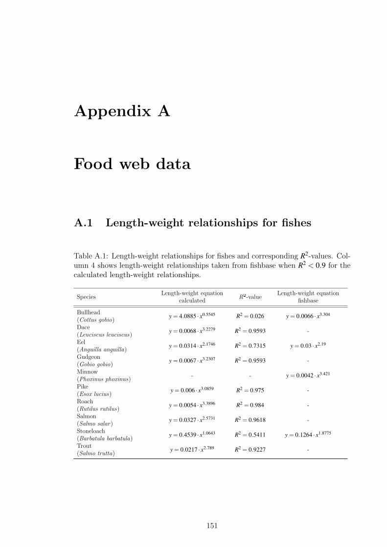
Appendix A

Food web data

A.1 Length-weight relationships for fishes

Table A.1: Length-weight relationships for fishes and corresponding R2-values. Col-umn 4 shows length-weight relationships taken from fishbase when R2 < 0.9 for thecalculated length-weight relationships.

SpeciesLength-weight equation

calculatedR²-value

Length-weight equationfishbase

Bullhead(Cottus gobio)

y = 4.0885 · x0.5545 R2 = 0.026 y = 0.0066 · x3.304

Dace(Leuciscus leuciscus)

y = 0.0068 · x3.2279 R2 = 0.9593 -

Eel(Anguilla anguilla)

y = 0.0314 · x2.1746 R2 = 0.7315 y = 0.03 · x2.19

Gudgeon(Gobio gobio)

y = 0.0067 · x3.2307 R2 = 0.9593 -

Minnow(Phoxinus phoxinus)

- - y = 0.0042 · x3.421

Pike(Esox lucius)

y = 0.006 · x3.0859 R2 = 0.975 -

Roach(Rutilus rutilus)

y = 0.0054 · x3.3896 R2 = 0.984 -

Salmon(Salmo salar)

y = 0.0327 · x2.5731 R2 = 0.9618 -

Stoneloach(Barbatula barbatula)

y = 0.4539 · x1.0643 R2 = 0.5411 y = 0.1264 · x1.8775

Trout(Salmo trutta)

y = 0.0217 · x2.789 R2 = 0.9227 -

151

A.2 Biomass data from macroinvertebrate sam-

ples

152

Table A.2: Macroinvertebrate biomass data from the in 2008 conducted survey. Themean total biomass was 12.32 g m−2.

Sample ID Date Patch ID Time Weight [g]

S01 30/07/2008 1 6:49 0.644S02 30/07/2008 2 6:56 0.259S03 30/07/2008 3 7:08 1.883S04 30/07/2008 4 7:14 0.070SO5 30/07/2008 5 7:21 0.949S06 30/07/2008 6 7:28 1.190S07 30/07/2008 1 12:26 1.027S08 30/07/2008 2 12:34 0.531S09 30/07/2008 3 12:40 0.918S10 30/07/2008 4 13:32 0.070S11 30/07/2008 5 13:25 1.269S12 30/07/2008 6 13:13 1.874S13 30/07/2008 1 19:09 0.964S14 30/07/2008 2 19:14 0.542S15 30/07/2008 3 19:20 1.353S16 30/07/2008 4 19:24 0.047S17 30/07/2008 5 19:52 0.751S18 30/07/2008 6 20:01 1.537S19 28/08/2008 1 7:05 0.536S20 28/08/2008 2 7:15 1.777S21 28/08/2008 3 7:55 1.413S22 28/08/2008 4 8:00 1.272S23 28/08/2008 5 8:10 2.106S24 28/08/2008 6 8:16 1.789S25 28/08/2008 1 12:25 1.635S26 28/08/2008 2 12:31 0.664S27 28/08/2008 3 12:36 1.770S28 28/08/2008 4 12:59 0.766S29 28/08/2008 5 13:08 2.917S30 28/08/2008 6 13:16 1.703S31 28/08/2008 1 19:20 1.894S32 28/08/2008 2 19:25 2.238S33 28/08/2008 3 19:33 2.366S34 28/08/2008 4 19:56 0.211S35 28/08/2008 5 20:03 1.452S36 28/08/2008 6 20:14 1.700

153

A.3 Food web nodes and starting stock values

Table A.3: Food web nodes, mean weight of the average individual (just fish nodes)and starting stock values.

Node Abbreviations Weight [g] Starting stock value[cal/m²]

Coleoptera Col 8Diptera Dip 603Ephemeroptera Eph 86Gammaridae Gam 5813Mollusca Mol 1147Oligochaeta Oli 1107Plecoptera Ple 1Trichoptera Tri 211Bullhead Bul 1.3 178Dace Dac 60.0 6681Eel 1 Ee1 24.6 1230Eel 2 Ee2 125.2 1381Eel 3 Ee3 148.1 2211Gudgeon Gud 35,7 329Minnow Min 1.7 2272Pike1 Pi1 97.6 270Pike2 Pi2 668.1 1108Pike3 Pi3 2216.9 4086Roach Roa 58.3 1128Salmon Sal 46.0 3231Stoneloach Sto 4.8 870Trout Tro 78.6 1924

154

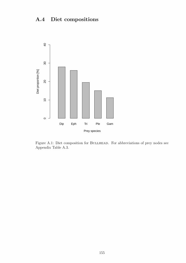
A.4 Diet compositions

Dip Eph Tri Ple Gam

Prey species

Die

t pro

port

ion

[%]

010

2030

40

Figure A.1: Diet composition for Bullhead. For abbreviations of prey nodes seeAppendix Table A.3.

155

Tri Eph Oli Mol Dip Gam

Prey species

Die

t pro

port

ion

[%]

020

4060

80

Figure A.2: Diet composition for Dace. For abbreviations of prey nodes see Ap-pendix Table A.3.

156

Gam Eph Tri Dip Col

Prey species

Die

t pro

port

ion

[%]

020

4060

8010

0

Figure A.3: Diet composition for Eel 1. For abbreviations of prey nodes see Ap-pendix Table A.3.

157

Bul Sto Tro Sal Ee1

Prey species

Die

t pro

port

ion

[%]

020

4060

8010

0


158

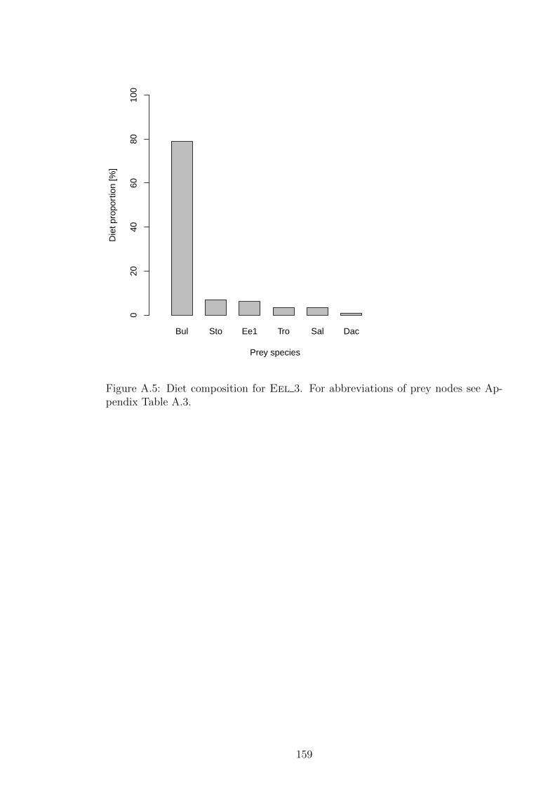
Bul Sto Ee1 Tro Sal Dac

Prey species

Die

t pro

port

ion

[%]

020

4060

8010

0


159

Gam Dip Tri Eph Mol Ple

Prey species

Die

t pro

port

ion

[%]

020

4060

80

Figure A.6: Diet composition for Gudgeon. For abbreviations of prey nodes seeAppendix Table A.3.

160

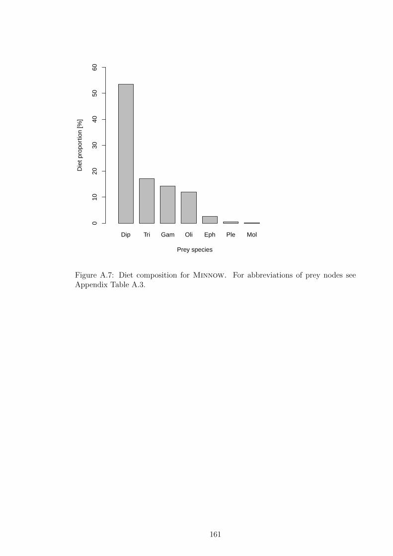
Dip Tri Gam Oli Eph Ple Mol

Prey species

Die

t pro

port

ion

[%]

010

2030

4050

60

Figure A.7: Diet composition for Minnow. For abbreviations of prey nodes seeAppendix Table A.3.

161

Min Sto Dac Gud Bul Sal Ee1

Prey species

Die

t pro

port

ion

[%]

010

2030

4050

60

Figure A.8: Diet composition for Pike1. For abbreviations of prey nodes see Ap-pendix Table A.3.

162

Min Dac Gud Sto Tro Bul Sal Roa Ee1 Pi1

Prey species

Die

t pro

port

ion

[%]

010

2030

40

Figure A.9: Diet composition for Pike2. For abbreviations of prey nodes see Ap-pendix Table A.3.

163

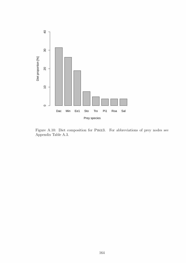
Dac Min Ee1 Sto Tro Pi1 Roa Sal

Prey species

Die

t pro

port

ion

[%]

010

2030

40

Figure A.10: Diet composition for Pike3. For abbreviations of prey nodes seeAppendix Table A.3.

164

Eph Tri Mol Dip

Prey species

Die

t pro

port

ion

[%]

010

2030

4050

60

Figure A.11: Diet composition for Roach. For abbreviations of prey nodes seeAppendix Table A.3.

165

Dip Tri Eph Gam Oli Ple Mol Col

Prey species

Die

t pro

port

ion

[%]

010

2030

4050

60

Figure A.12: Diet composition for Salmon. For abbreviations of prey nodes seeAppendix Table A.3.

166

Dip Gam Ple Eph Tri

Prey species

Die

t pro

port

ion

[%]

020

4060

80

Figure A.13: Diet composition for Stoneloach. For abbreviations of prey nodessee Appendix Table A.3.

167

Dip Tri Gam Oli Eph Ple Col Mol

Prey species

Die

t pro

port

ion

[%]

010

2030

4050

60

Figure A.14: Diet composition for Trout. For abbreviations of prey nodes seeAppendix Table A.3.

168

A.5 Additional energy input

Table A.4: Additional energy input that is used for removal experiments. Additionalinput is the value that was added to the value obtained from calculating energydemand from the metabolic rate. The last column shows the percentage that wasadded to the the calculated input based on the metabolic rate.

Species node Additionalinput

Total inputfrom the

environment

Input formthe

environmentbased on MR

(justinvertebrates)

Addedpercentage of

metabolicrate [%]

Coleoptera 6.3 7 0.7 903Diptera 58 85 27 216Ephemeroptera 53.4 60 6.6 811Gammaridae 30 400 370 8Mollusca -33 350 383 -9Oligochaeta 11 70 59 19Plecoptera 7.9 8 0.1 14138Trichoptera 88 100 12 724Bullhead 20 20 312Salmon 3 3 5Trout 3 3 9Minnow 15 15 19Stoneloach 8 8 33Dace 5 5 4Gudgeon 0 0 0Roach 0 0 0Pike1 1 1 23Pike2 1 1 8Pike3 3 3 8Eel 1 10 10 39Eel 2 5 5 23Eel 3 5 5 15

169

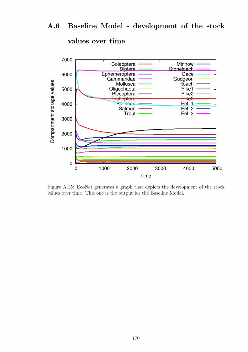
A.6 Baseline Model - development of the stock

values over time

0

1000

2000

3000

4000

5000

6000

7000

0 1000 2000 3000 4000 5000

Co

mp

art

me

nt

sto

rag

e v

alu

es

Time

ColeopteraDiptera

EphemeropteraGammaridae

MolluscaOligochaetaPlecopteraTrichoptera

BullheadSalmon

Trout

MinnowStoneloach

DaceGudgeon

RoachPike1Pike2Pike3Eel_1Eel_2Eel_3

Figure A.15: EcoNet generates a graph that depicts the development of the stockvalues over time. This one is the output for the Baseline Model.

170

Appendix B

Methods of gut content analysis

171

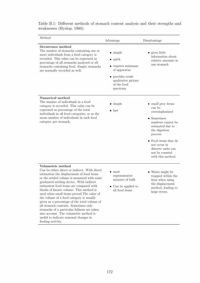
Table B.1: Different methods of stomach content analysis and their strengths andweaknesses (Hyslop, 1980).

MethodAdvantage Disadvantage

Occurrence methodThe number of stomachs containing one ormore individuals from a food category isrecorded. This value can be expressed aspercentage of all stomachs analysed or allstomachs containing food. Empty stomachsare normally recorded as well.

simple

quick

requires minimumof apparatus

provides crudequalitative pictureof the foodspectrum.

gives littleinformation aboutrelative amounts inone stomach

Numerical methodThe number of individuals in a foodcategory is recorded. This value can beexpressed as percentage of the totalindividuals in all food categories, or as themean number of individuals in each foodcategory per stomach.

simple

fast

small prey itemscan beoveremphasized

Sometimesnumbers cannot beestimated due tothe digestionprocess.

Food items that donot occur indiscrete units cannot be countedwith this method.

Volumetric methodCan be either direct or indirect. With directestimation the displacement of food itemsor the settled volume is measured with somegraduated settling device. With indirectestimation food items are compared withblocks of known volume. This method isused when small items prevail.The value ofthe volume of a food category is usuallygiven as a percentage of the total volume ofall stomach contents. Sometimes onlystomachs of a particular fullness are takeninto account. The volumetric method isuseful to indicate seasonal changes infeeding activity.

mostrepresentativemeasure of bulk

Can be applied toall food items

Water might betrapped within theitem when usingthe displacementmethod, leading tolarge errors.

172

Appendix C

Model parameters and methods

C.1 Methods for the calculation of the differential

equations

The user has got the choice of method between i) Adaptive Time Step (Runge-

Kutta-Fehlberg), ii) Fixed Time Step (4th order Runge-Kutta) and iii) Stochastic

(Langevin) method to solve the differential equations. The Adaptive Time Step and

the Fixed Time Step methods are both deterministic methods, i.e producing the

same output with identical starting conditions.

Adaptive Time Step: The Adaptive Time Step method continuously adjusts

the accuracy for the numerical solution of the differential equations based on the

complexity of the differential equations. The amount of error allowed between the

actual solution and the numerical solution is defined by the Sensitivity parameter,

which can be adjusted by the the user. Smaller values for Sensitivity are more

accurate, but require longer computation time. In many cases a higher Sensitivity

parameter does not change the final steady state. The parameter Maximum Time

defines the simulation length.

173

Fixed Time Step: In comparison to the adaptive time step method, the fixed

step method does not adjust its accuracy, but is fixed by the parameter Step-size

throughout the simulation. Step-size complies with the Sensitivity parameter, be-

cause both are a limit of the allowed error. The adaptive time step method is

favoured over the fixed time step method, because it is generally faster and more

accurate. However, there might be cases when the user needs more control over the

numerical solution. Instead of Maximum Time the parameter for simulation length

is called Total Time.

Stochastic: Stochastic methods incorporate probabilistic behaviour and generates

different solutions on each occasion. The adjustable parameters are the same as for

the fixed time step method. Only systems that are probabilistic in nature (e.g.

ecosystems) should be modelled with this method. The strength of this method

is that it shows different outcomes to identical starting conditions, providing an

indication whether there is more than one stable state for the system. The stochastic

method used by EcoNet is based on the Langevin equation (Gillespie, 2000). It is

a true stochastic method and should not be confused with a deterministic solution

with added noise (Gardiner, 1985; Gillespie, 1992; 2000).

For the removal experiments the adaptive time step method was chosen. Simulations

were run with the Baseline Model to assess the influence of model parameters such

as time steps and sensitivity.

C.2 Model parametrisation

Max Time Steps parameter The calculations in the model are based on time

steps. Therefore flow rates have to be normalised to the same timescale (e.g. daily

consumption). The output of the model that depicts the values of the compartments

over time should not be confused with a projection of the development of stock values

over a certain period (e.g. year), but rather indicates if the system reaches a stable

174

state, which is necessary to proceed with species removal. In the real food web

species abundance changes seasonally, but in the model mean values over the year

are used. Therefore, seasonal patterns are not reflected. The model will predict how

the removal of species propagates through the system and how that influences the

abundance of other species. It does not attempt to give an account of the exact

development of species abundance on a day to day scale.

The choice of time steps mainly depends on when the stable state is reached. Stop-

ping the simulation at an earlier point might result in different values. The parameter

Max Time Steps was adjusted accordingly in all modelling trials.

Sensitivity parameter The Adaptive Time Step method continuously adjusts

its accuracy based on the complexity of the differential equations. The amount of

error allowed is defined by the Sensitivity parameter, which can be adjusted by the

the user, before the model is run. Smaller values for Sensitivity are more accurate,

but require longer computation time. The Baseline Model without additional energy

input was run with sensitivity values of 0.01, 0.05, 0.1, and 10.0, but no influence

on the final stock values was found.

C.3 Energy assimilation efficiency

The energy available to the organism is dependent on the digestion efficiency of

a particular food source, the rest is excreted as faeces. An organism invests that

energy into: maintenance, digestion, activity, growth , allocation of reserves, and

reproduction. Only the energy invested into biomass is available to the next higher

trophic level. In general only 5 to 20% of the energy of one trophic level is available

to the next trophic level (Cragg, 1969; White, 1992). In the model this is reflected by

an outflow rate from each organism into the environment. The range of the outflow

rate (80 to 95% of the stock value) provides room for adjustments to stabilise the

model. The removals are run with 90% assimilation efficiency for all species. The

outflow rate is calculated in the following way:

175

cout f low = 0.9 · IA , with A: starting stock value predator [cal], I: ingestion rate [cal d m−2].

Variation of energy assimilation efficiency Dependent on the food source this

assimilation energy may vary. To assess the influence of higher assimilation rates

the Baseline Model (without additional energy input) was run with outflow rates

based on 20 and 30 % assimilation rates. In the model runs with higher assimilation

efficiency most of the energy gets assigned to Pike2, but also Trout benefits. The

model was also run with mixed outflow rates. Variation of the energy assimilation

efficiency did not result in less extinctions and was not sufficient to achieve a model

output that resembles the original food web closely enough.

176

Appendix D

Additional results for removals

D.1 Removals from the natural communities

177

Autumn 2003

Figure D.1: MDS-ordination for removals from baseline community Autumn ’03.For abbreviations of prey nodes see Appendix Table A.3. Stress: 10.25%.

178

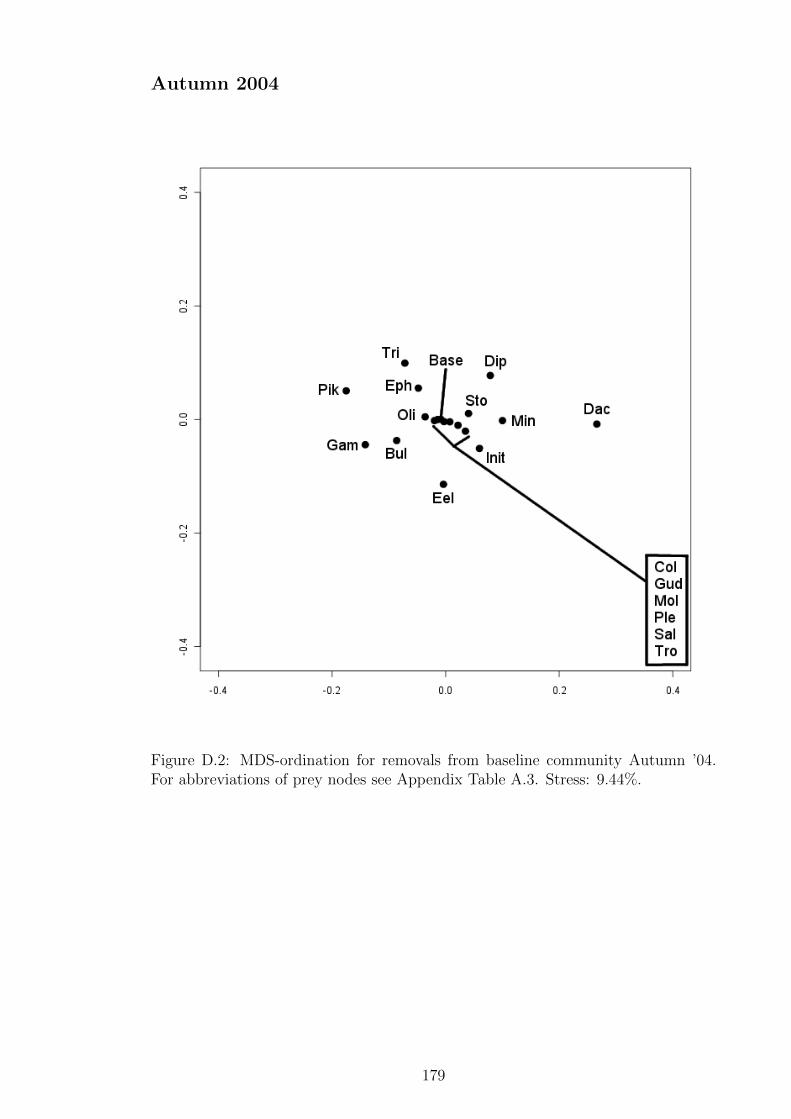
Autumn 2004


179

Autumn 2005


180

D.2 Relative change of abundance in the remain-

ing nodes after species removal

Coleoptera removal

Dip

Eph

Gam M

ol Oli

Ple Tr

iB

ulD

acE

e1E

e2E

e3G

ud Min

Pi1

Pi2

Pi3

Roa Sal

Sto Tro

Diff

eren

ce in

abu

ndan

ce [%

]

−100

−50

0

50

100

Mollusca removal

Col

Dip

Eph

Gam O

liP

le Tri

Bul

Dac

Ee1

Ee2

Ee3

Gud Min

Pi1

Pi2

Pi3

Roa Sal

Sto Tro

Diff

eren

ce in

abu

ndan

ce [%

]

−100

−50

0

50

100

Oligochaeta removal

Col

Dip

Eph

Gam M

olP

le Tri

Bul

Dac

Ee1

Ee2

Ee3

Gud Min

Pi1

Pi2

Pi3

Roa Sal

Sto Tro

Diff

eren

ce in

abu

ndan

ce [%

]

−100

−50

0

50

100

Plecoptera removal

Col

Dip

Eph

Gam M

ol Oli

Tri

Bul

Dac

Ee1

Ee2

Ee3

Gud Min

Pi1

Pi2

Pi3

Roa Sal

Sto Tro

Diff

eren

ce in

abu

ndan

ce [%

]

−100

−50

0

50

100

Figure D.4: Impact of the removal of the macroinvertebrate nodes Coleoptera,Mollusca, Oligochaeta and Plecoptera on the abundance of the remainingnodes, relative to the Baseline model. For abbreviations of prey nodes see AppendixTable A.3.

181

Diptera removal

Col

Eph

Gam M

ol Oli

Ple Tr

iB

ulD

acE

e1E

e2E

e3G

ud Min

Pi1

Pi2

Pi3

Roa Sal

Sto Tro

Diff

eren

ce in

abu

ndan

ce [%

]

−100

−50

0

50

100

Ephemeroptera removal

Col

Dip

Gam M

ol Oli

Ple Tr

iB

ulD

acE

e1E

e2E

e3G

ud Min

Pi1

Pi2

Pi3

Roa Sal

Sto Tro

Diff

eren

ce in

abu

ndan

ce [%

]

−100

−50

0

50

100

Gammaridae removal

Col

Dip

Eph Mol Oli

Ple Tr

iB

ulD

acE

e1E

e2E

e3G

ud Min

Pi1

Pi2

Pi3

Roa Sal

Sto Tro

Diff

eren

ce in

abu

ndan

ce [%

]

−100

−50

0

50

100

Trichoptera removal

Col

Dip

Eph

Gam M

ol Oli

Ple

Bul

Dac

Ee1

Ee2

Ee3

Gud Min

Pi1

Pi2

Pi3

Roa Sal

Sto Tro

Diff

eren

ce in

abu

ndan

ce [%

]

−100

−50

0

50

100

Figure D.5: Impact of the removal of the macroinvertebrate nodes Diptera,Ephemeroptera, Gammaridae and Trichoptera on the abundance of theremaining nodes, relative to the Baseline model. For abbreviations of prey nodessee Appendix Table A.3.

182

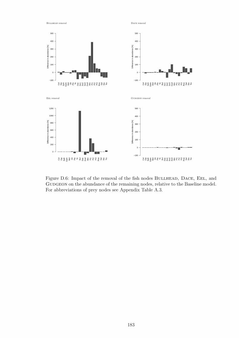
Bullhead removal

Col

Dip

Eph

Gam M

ol Oli

Ple Tr

iD

acE

e1E

e2E

e3G

ud Min

Pi1

Pi2

Pi3

Roa Sal

Sto Tro

Diff

eren

ce in

abu

ndan

ce [%

]

−100

0

100

200

300

400

500

Dace removal

Col

Dip

Eph

Gam M

ol Oli

Ple Tr

iB

ulE

e1E

e2E

e3G

ud Min

Pi1

Pi2

Pi3

Roa Sal

Sto Tro

Diff

eren

ce in

abu

ndan

ce [%

]

−100

0

100

200

300

400

500

Eel removal

Col

Dip

Eph

Gam M

ol Oli

Ple Tr

iB

ulD

acG

ud Min

Pi1

Pi2

Pi3

Roa Sal

Sto Tro

Diff

eren

ce in

abu

ndan

ce [%

]

0

200

400

600

800

1000

1200

Gudgeon removal

Col

Dip

Eph

Gam M

ol Oli

Ple Tr

iB

ulD

acE

e1E

e2E

e3 Min

Pi1

Pi2

Pi3

Roa Sal

Sto Tro

Diff

eren

ce in

abu

ndan

ce [%

]

−100

0

100

200

300

400

500

Figure D.6: Impact of the removal of the fish nodes Bullhead, Dace, Eel, andGudgeon on the abundance of the remaining nodes, relative to the Baseline model.For abbreviations of prey nodes see Appendix Table A.3.

183

Minnow removal

Col

Dip

Eph

Gam M

ol Oli

Ple Tr

iB

ulD

acE

e1E

e2E

e3G

ud Pi1

Pi2

Pi3

Roa Sal

Sto Tro

Diff

eren

ce in

abu

ndan

ce [%

]

−100

0

100

200

300

400

500

Pike removal

Col

Dip

Eph

Gam M

ol Oli

Ple Tr

iB

ulD

acE

e1E

e2E

e3G

ud Min

Roa Sal

Sto Tro

Diff

eren

ce in

abu

ndan

ce [%

]

−100

0

100

200

300

400

500

Roach removal

Col

Dip

Eph

Gam M

ol Oli

Ple Tr

iB

ulD

acE

e1E

e2E

e3G

ud Min

Pi1

Pi2

Pi3

Sal

Sto Tro

Diff

eren

ce in

abu

ndan

ce [%

]

−100

0

100

200

300

400

500

Salmon removal

Col

Dip

Eph

Gam M

ol Oli

Ple Tr

iB

ulD

acE

e1E

e2E

e3G

ud Min

Pi1

Pi2

Pi3

Roa Sto Tro

Diff

eren

ce in

abu

ndan

ce [%

]

−100

0

100

200

300

400

500

Figure D.7: Impact of the removal of the fish nodes Minnow, Pike, Roach andSalmon on the abundance of the remaining nodes, relative to the Baseline model.For abbreviations of prey nodes see Appendix Table A.3.

184

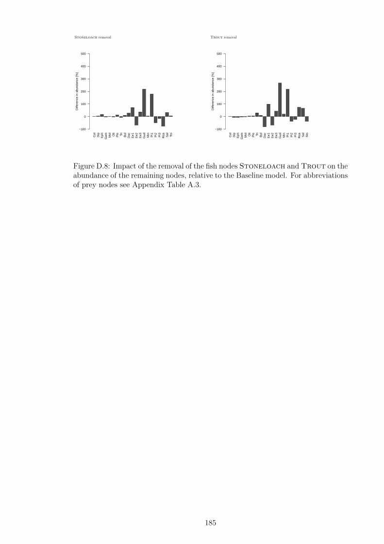
Stoneloach removal

Col

Dip

Eph

Gam M

ol Oli

Ple Tr

iB

ulD

acE

e1E

e2E

e3G

ud Min

Pi1

Pi2

Pi3

Roa Sal

Tro

Diff

eren

ce in

abu

ndan

ce [%

]

−100

0

100

200

300

400

500

Trout removal

Col

Dip

Eph

Gam M

ol Oli

Ple Tr

iB

ulD

acE

e1E

e2E

e3G

ud Min

Pi1

Pi2

Pi3

Roa Sal

Sto

Diff

eren

ce in

abu

ndan

ce [%

]

−100

0

100

200

300

400

500

Figure D.8: Impact of the removal of the fish nodes Stoneloach and Trout on theabundance of the remaining nodes, relative to the Baseline model. For abbreviationsof prey nodes see Appendix Table A.3.

185

Bibliography

Abarca-Arenas, L. G. and Ulanowicz, R. E. (2002). The effects of taxonomic aggre-

gation on network analysis. Ecological Modelling, 149(3):285–296.

Adamicka, P. S. (1991). A Food Schedule for Cottus-Gobio L (Pisces) in Oberer-

Seebach, Ritrodat-Lunz Study Area, Austria. International Association of Theo-

retical and Applied Limnology, 24:1941–1943.

Adams, J. (1993). A review of the NRA Anglian Region Zander Cull Policy. Unpub-

lished document available from Environment Agency, Kingfisher House, Goldhay

Way, Orton Goldhay, Peterborough PE2 0ZR, United Kingdom.

Akbari, M., Murphy, S., Kay, J., and Swanton, C. (1999). Energy-Bases Indicators

of (Agro)Ecosystem Health. In Quattrochi, D. and Luvall, J., editors, Thermal

Remote sensing in Land Surface Processes. Ann Arbor Press.

Allan, J. D. (2004). Landscapes and riverscapes: The influence of land use on stream

ecosystems. Annual Review of Ecology Evolution and Systematics, 35:257–284.

Allan, J. D., Palmer, M., and Poff, N. L. (2005). Climate change and freshwater

ecosystems. In Climate change and biodiversity, pages 274–295. Yale University

Press, New Haven & London.

Allesina, S., Bondavalli, C., and Scharler, U. M. (2005). The consequences of the

aggregation of detritus pools in ecological networks. Ecological Modelling, 189:221–

232.

Amoros, C., Rostan, J. C., Pautou, G., and Bravard, J. P. (1987). The reversible

186

process concept applied to the environmental-management of large river systems.

Environmental Management, 11(5):607–617.

Anderson, M. J. and Willis, T. J. (2003). Canonical analysis of principal coordinates:

A useful method of constrained ordination for ecology. Ecology, 84(2):511–525.

Arlinghaus, R., Mehner, T., and Cowx, I. G. (2002). Reconciling traditional inland

fisheries management and sustainability in industrialized countries, with emphasis

on Europe. Fish and Fisheries, 3(4):261–316.

Atkinson, D. (1994). Temperature and Organism Size - A Biological Law For Ec-

totherms. Advances In Ecological Research, Vol 25, 25:1–58.

Baensch, H. and Riehl, R. (1991). Aquarien atlas, volume Bd. 3. Mergus, Verlag fur

Natur- und Heimtierkunde, Melle, Germany.

Baird, D., Fath, B. D., Ulanowicz, R. E., Asmus, H., and Asmus, R. (2009). On

the consequences of aggregation and balancing of networks on system properties

derived from ecological network analysis. Ecological Modelling, 220(23):3465–3471.

Balvanera, P., Pfisterer, A. B., Buchmann, N., He, J. S., Nakashizuka, T., Raffaelli,

D., and Schmid, B. (2006). Quantifying the evidence for biodiversity effects on

ecosystem functioning and services. Ecology Letters, 9(10):1146–1156.

Baras, E. (1994). Constraints Imposed By High-densities On Behavioral Spawning

Strategies In the Barbel, Barbus-barbus. Folia Zoologica, 43(3):255–266.

Baron, J. S., Poff, N. L., Angermeier, P. L., Dahm, C. N., Gleick, P. H., Hairston,

N. G., Jackson, R. B., Johnston, C. A., Richter, B. D., and Steinman, A. D.

(2002). Meeting ecological and societal needs for freshwater. Ecological Applica-

tions, 12(5):1247–1260.

Baxter, C. V., Fausch, K. D., Murakami, M., and Chapman, P. L. (2004). Fish

invasion restructures stream and forest food webs by interrupting reciprocal prey

subsidies. Ecology, 85(10):2656–2663.

187

Baxter, C. V., Fausch, K. D., and Saunders, W. C. (2005). Tangled webs: reciprocal

flows of invertebrate prey link streams and riparian zones. Freshwater Biology,

50(2):201–220.

Bejan, A. (1997). Advanced Engineering Thermodynamics. John Wiley and sons,

New York.

Belgrano, A., Scharler, U. M., Dunne, J., and Ulanowicz, R. E. (2005). Aquatic Food

Webs An Ecosystem Approach. Oxford University Press.

Bender, E. A., Case, T. J., and Gilpin, M. E. (1984). Perturbation Experiments In

Community Ecology - Theory and Practice. Ecology, 65(1):1–13.

Bengtsson, J., Angelstam, P., Elmqvist, T., Emanuelsson, U., Folke, C., Ihse, M.,

Moberg, F., and Nystrom, M. (2003). Reserves, resilience and dynamic landscapes.

Ambio, 32(6):389–396.

Benke, A. C. (1993). Concepts and Patterns of Invertebrate Production In Run-

ning Waters. International Association of Theoretical and Applied Limnology -

Proceedings, Vol 25, Pt 1, 25:15–38.

Benke, A. C. (1998). Production dynamics of riverine chironomids: Extremely high

biomass turnover rates of primary consumers. Ecology, 79(3):899–910.

Benke, A. C., Hauer, F. R., Stites, D. L., Meyer, J. L., and Edwards, R. T. (1992).

Growth of Snag-dwelling Mayflies In A Blackwater River - the Influence of Tem-

perature and Food. Archiv Fur Hydrobiologie, 125(1):63–81.

Benke, A. C., Huryn, A. D., Smock, L. A., and Wallace, J. B. (1999). Length-mass

relationships for freshwater macroinvertebrates in North America with particular

reference to the southeastern United States. J. N. Am. Benthol. Soc., 18(3):308–

343.

Benke, A. C. and Wallace, J. B. (1997). Trophic basis of production among riverine

caddisflies: Implications for food web analysis. Ecology, 78(4):1132–1145.

188

Benstead, J. P., March, J. G., Pringle, C. M., Ewel, K. C., and Short, J. W. (2009).

Biodiversity and ecosystem function in species-poor communities: community

structure and leaf litter breakdown in a Pacific island stream. Journal of the

North American Benthological Society, 28(2):454–465.

Berg, L. (1964). Freshwater fishes of the U.S.S.R. and adjacent countries, volume 2.

Israel Program for Scientific Translations Ltd, Jerusalem, 4 edition.

Berlow, E. L. (1999). Strong effects of weak interactions in ecological communities.

Nature, 398(6725):330.

Berlow, E. L., Brose, U., and Martinez, N. D. (2008). The ”Goldilocks factor” in

food webs. Proceedings of the National Academy of Sciences of the United States

of America, 105(11):4079–4080.

Berlow, E. L., Navarrete, S. A., Briggs, C. J., Power, M. E., and Menge, B. A.

(1999). Quantifying variation in the strengths of species interactions. Ecology,

80(7):2206–2224.

Berlow, E. L., Neutel, A. M., Cohen, J. E., de Ruiter, P. C., Ebenman, B., Emmer-

son, M., Fox, J. W., Jansen, V. A. A., Jones, J. I., Kokkoris, G. D., Logofet, D. O.,

McKane, A. J., Montoya, J. M., and Petchey, O. (2004). Interaction strengths in

food webs: issues and opportunities. Journal of Animal Ecology, 73(3):585–598.

Berrie, A. (1976). Detritus microorganisms and animals in fresh water. In Anderson,

J. M. and Macfadyen, A., editors, The Role Of Terrestrial And Aquatic Organ-

isms In Decomposition Processes, volume 17, page 1977, Oxford, England. British

Ecological Society Symposium, Blackwell Scientific Publications.

Berrie, A. D. (1992). The Chalk-Stream Environment. Hydrobiologia, 248(1):3–9.

Berryman, A. A. (1991). Stabilization Or Regulation - What It All Means. Oecologia,

86(1):140–143.

Bianco, P. G. (1998). Diversity of Barbinae fishes in southern Europe with descrip-

189

tion of a new genus and a new species (Cyprinidae). Italian Journal of Zoology,

65(1 supp 1):125–136.

Bianco, P. G. and Ketmaier, V. (2001). Anthropogenic changes in the freshwater fish

fauna of Italy, with reference to the central region and Barbus graellsii, a newly

established alien species of Iberian origin. Journal of Fish Biology, 59:190–208.

Blanc, G. (1997). Introduced pathogens in European aquatic ecosystems: Theo-

retical aspects and realities. Bulletin Francais de la Peche et de la Pisciculture,

(344-45):489–513.

Blanchet, S., Grenouillet, G., Beauchard, O., Tedesco, P. A., Leprieur, F., Durr,

H. H., Busson, F., Oberdorff, T., and Brosse, S. (2010). Non-native species disrupt

the worldwide patterns of freshwater fish body size: implications for Bergmann’s

rule. Ecology Letters, 13(4):421–431.

Blindow, I., Andersson, G., Hargeby, A., and Johansson, S. (1993). Long-term

Pattern of Alternative Stable States In 2 Shallow Eutrophic Lakes. Freshwater

Biology, 30(1):159–167.

Blondel, J. (2003). Guilds or functional groups: does it matter? Oikos, 100(2):223–

231.

Bond, N. R., Lake, P. S., and Arthington, A. H. (2008). The impacts of drought on

freshwater ecosystems: an Australian perspective. Hydrobiologia, 600:3–16.

Bond, W. J. (1993). In Biodiversity and ecosystem function, pages 237–253. Springer-

Verlag, Berlin, Germany.

Borer, E. T., Anderson, K., Blanchette, C. A., Broitman, B., Cooper, S. D., Halpern,

B. S., Seabloom, E. W., and Shurin, J. B. (2002). Topological approaches to food

web analyses: a few modifications may improve our insights. Oikos, 99(2):397–401.

Borer, E. T., Seabloom, E. W., Shurin, J. B., Anderson, K. E., Blanchette, C. A.,

Broitman, B., Cooper, S. D., and Halpern, B. S. (2005). What determines the

strength of a trophic cascade? Ecology, 86(2):528–537.

190

Borrvall, C., Ebenman, B., and Jonsson, T. (2000). Biodiversity lessens the risk of

cascading extinction in model food webs. Ecology Letters, 3(2):131–136.

Bracken, M. E. S. and Stachowicz, J. J. (2006). Seaweed diversity enhances nitrogen

uptake via complementary use of nitrate and ammonium. Ecology, 87(9):2397–

2403.

Brander, K. M. (1995). The Effect Of Temperature On Growth Of Atlantic Cod

(Gadus-Morhua L). Ices Journal Of Marine Science, 52(1):1–10.

Britton, J. R., Brazier, M., Davies, G. D., and Chare, S. I. (2008). Case studies on

eradicating the Asiatic cyprinid Pseudorasbora parva from fishing lakes in England

to prevent their riverine dispersal. Aquatic Conservation-marine and Freshwater

Ecosystems, 18(6):867–876.

Britton, J. R., Cucherousset, J., Davies, G. D., Godard, M. J., and Copp, G. H.

(2010a). Non-native fishes and climate change: predicting species responses to

warming temperatures in a temperate region. Freshwater Biology, 55(5):1130–

1141.

Britton, J. R., Cucherousset, J., Grey, J., and Gozlan, R. E. (2011). Determining

the strength of exploitative competition from an introduced fish: roles of density,

biomass and body size. Ecology of Freshwater Fish, 20(1):74–79.

Britton, J. R., Davies, G. D., and Brazier, M. (2010b). Towards the successful

control of the invasive Pseudorasbora parva in the UK. Biological Invasions,

12(1):125–131.

Britton, J. R., Davies, G. D., Brazier, M., and Pinder, A. C. (2007). A case study on

the population ecology of a topmouth gudgeon (Pseudorasbora parva) population

in the UK and the implications for native fish communities. Aquatic Conservation-

marine and Freshwater Ecosystems, 17(7):749–759.

Britton, J. R., Davies, G. D., and Harrod, C. (2010c). Trophic interactions and

consequent impacts of the invasive fish Pseudorasbora parva in a native aquatic

foodweb: a field investigation in the UK. Biological Invasions, 12(6):1533–1542.

191

Brown, J. H., Gillooly, J. F., Allen, A. P., Savage, V. M., and West, G. B. (2004).

Toward a metabolic theory of ecology. Ecology, 85(7):1771–1789.

Brzustowski, T. A. and Golem, P. J. (1977). 2nd-law Analysis of Energy Processes

.1. Exergy - Introduction. Transactions of the Canadian Society For Mechanical

Engineering, 4(4):209–218.

Bystrom, P., Karlsson, J., Nilsson, P., Van Kooten, T., Ask, J., and Olofsson, F.

(2007). Substitution of top predators: effects of pike invasion in a subarctic lake.

Freshwater Biology, 52(7):1271–1280.

Cairns, J. (1977). Quantification of biological integrity. In Ballentine, R. K.; Guar-

raia, L. J., editor, The integrity of water, pages 171–187. U.S. Environmental

Protection Agency, Office of Water and Hazardous Materials, Washington, D.C.,

USA.

Cardinale, B. J., Nelson, K., and Palmer, M. A. (2000). Linking species diversity

to the functioning of ecosystems: on the importance of environmental context.

Oikos, 91(1):175–183.

Cardinale, B. J., Palmer, M. A., Ives, A. R., and Brooks, S. S. (2005). Diversity-

productivity relationships in streams vary as a function of the natural disturbance

regime. Ecology, 86(3):716–726.

Cardinale, B. J., Wright, J. P., Cadotte, M. W., Carroll, I. T., Hector, A., Srivas-

tava, D. S., Loreau, M., and Weis, J. J. (2007). Impacts of plant diversity on

biomass production increase through time because of species complementarity.

Proceedings of the National Academy of Sciences of the United States of America,

104(46):18123–18128.

Carpenter, S. R. (1996a). Drivers and dynamics of changes in biodiversity. In

(UNEP), U. N. E. P., editor, Global biodiversity assessment, pages 311–318. Cam-

bridge University Press, Cambridge, United Kingdom.

Carpenter, S. R. (1996b). Microcosm experiments have limited relevance for com-

munity and ecosystem ecology. Ecology, 77(3):677–680.

192

Carpenter, S. R. and Cottingham, K. L. (1997). Resilience and restoration of lakes.

Conservation Ecology (online), 1(1).

Carpenter, S. R. and Kitchell, J. F. (1996). The Trophic Cascade in Lakes. Cam-

bridge University Press.

Carpenter, S. R. and Lodge, D. M. (1986). Effects of Submersed Macrophytes On

Ecosystem Processes. Aquatic Botany, 26(3-4):341–370.

Carpenter, S. R., Ludwig, D., and Brock, W. A. (1999). Management of eutrophi-

cation for lakes subject to potentially irreversible change. Ecological Applications,

9(3):751–771.

Cederholm, C. J., Kunze, M. D., Murota, T., and Sibatani, A. (1999). Pacific

salmon carcasses: Essential contributions of nutrients and energy for aquatic and

terrestrial ecosystems. Fisheries, 24(10):6–15.

Chapin, F. S., Walker, B. H., Hobbs, R. J., Hooper, D. U., Lawton, J. H., Sala,

O. E., and Tilman, D. (1997). Biotic control over the functioning of ecosystems.

Science, 277(5325):500–504.

Chapin, F. S., Zavaleta, E. S., Eviner, V. T., Naylor, R. L., Vitousek, P. M.,

Reynolds, H. L., Hooper, D. U., Lavorel, S., Sala, O. E., Hobbie, S. E., Mack,

M. C., and Diaz, S. (2000). Consequences of changing biodiversity. Nature,

405(6783):234–242.

Clarke, A. (1993). Temperature And Extinction In The Sea - A Physiologists View.

Paleobiology, 19(4):499–518.

Cohen, J. E., Beaver, R. A., Cousins, S. H., Deangelis, D. L., Goldwasser, L., Heong,

K. L., Holt, R. D., Kohn, A. J., Lawton, J. H., Martinez, N., Omalley, R., Page,

L. M., Patten, B. C., Pimm, S. L., Polis, G. A., Rejmanek, M., Schoener, T. W.,

Schoenly, K., Sprules, W. G., Teal, J. M., Ulanowicz, R. E., Warren, P. H., Wilbur,

H. M., and Yodzis, P. (1993). Improving Food Webs. Ecology, 74(1):252–258.

193

Collares-Pereira, M. J., Martins, M. J., Pires, A. M., Geraldes, A. M., and Coelho,

M. M. (1996). Feeding behaviour of Barbus bocagei assessed under a spatio-

temporal approach. Folia Zoologica, 45(1):65–76.

Collins, P. T. (1992). Length Biomass Relationships for Terrestrial Gastropoda and

Oligochaeta. American Midland Naturalist, 128(2):404–406.

Cooke, S. J. and Cowx, I. G. (2004). The role of recreational fishing in global fish

crises. Bioscience, 54(9):857–859.

Cooper, S. D., Walde, S. J., and Peckarsky, B. L. (1990). Prey Exchange-rates and

the Impact of Predators On Prey Populations In Streams. Ecology, 71(4):1503–

1514.

Copp, G. H., Bianco, P. G., Bogutskaya, N. G., Eros, T., Falka, I., Ferreira, M. T.,

Fox, M. G., Freyhof, J., Gozlan, R. E., Grabowska, J., Kovac, V., Moreno-Amich,

R., Naseka, A. M., Penaz, M., Povz, M., Przybylski, M., Robillard, M., Russell,

I. C., Stakenas, S., Sumer, S., Vila-Gispert, A., and Wiesner, C. (2005a). To

be, or not to be, a non-native freshwater fish? Journal of Applied Ichthyology,

21(4):242–262.

Copp, G. H., Garthwaite, R., and Gozlan, R. E. (2005b). Risk identification and as-

sessment of non-native freshwater fishes: a summary of concepts and perspectives

on protocols for the UK. Journal of Applied Ichthyology, 21(4):371–373.

Copp, G. H., Spathari, S., and Turmel, M. (2005c). Consistency of Diel behaviour

and interactions of stream fishes and invertebrates during summer. River Research

and Applications, 21(1):75–90.

Copp, G. H., Templeton, M., and Gozlan, R. E. (2007). Propagule pressure and the

invasion risks of non-native freshwater fishes: a case study in England. Journal

Of Fish Biology, 71:148–159.

Copp, G. H., Vilizzi, L., and Gozlan, R. E. (2010a). The demography of introduction

pathways, propagule pressure and occurrences of non-native freshwater fish in

194

England. Aquatic Conservation-marine and Freshwater Ecosystems, 20(5):595–

601.

Copp, G. H., Vilizzi, L., and Gozlan, R. E. (2010b). Fish movements: the in-

troduction pathway for topmouth gudgeon Pseudorasbora parva and other non-

native fishes in the UK. Aquatic Conservation-marine and Freshwater Ecosystems,

20(3):269–273.

Copp, G. H., Wesley, K. J., and Vilizzi, L. (2005d). Pathways of ornamental and

aquarium fish introductions into urban ponds of Epping Forest (London, Eng-

land): the human vector. Journal of Applied Ichthyology, 21(4):263–274.

Costanza, R., dArge, R., deGroot, R., Farber, S., Grasso, M., Hannon, B., Limburg,

K., Naeem, S., ONeill, R. V., Paruelo, J., Raskin, R. G., Sutton, P., and vanden-

Belt, M. (1997). The value of the world’s ecosystem services and natural capital.

Nature, 387(6630):253–260.

Coutant, C. C. (1987). Thermal Preference - When Does An Asset Become A

Liability. Environmental Biology of Fishes, 18(3):161–172.

Covich, A. P., Austen, M. C., Barlocher, F., Chauvet, E., Cardinale, B. J., Biles,

C. L., Inchausti, P., Dangles, O., Solan, M., Gessner, M. O., Statzner, B., and

Moss, B. (2004). The role of Biodiversity in the functioning of freshwater and

marine benthic ecosystems. Bioscience, 54(8):767–775.

Creed, R. P. (2006). Predator transitions in stream communities: a model and

evidence from field studies. Journal of the North American Benthological Society,

25(3):533–544.

Crisp, D. M. A. and Westlake, D. (1982). The temperatures of nine flowing waters

in southern England. Hydrobiologia, 89:193–204.

Crowder, L. B. and Cooper, W. E. (1982). Habitat Structural Complexity and the

Interaction Between Bluegills and Their Prey. Ecology, 63(6):1802–1813.

195

Cummins, K. W. (1974). Structure and Function of Stream Ecosystems. Bioscience,

24(11):631–641.

Cummins, K. W. and Wuycheck, J. C. (1971). Caloric Equivalents for Investigations

in Ecological Energetics. Schweizerbart’sche Verlagsbuchhandling.

Cury, P., Bakun, A., Crawford, R. J. M., Jarre, A., Quinones, R. A., Shannon,

L. J., and Verheye, H. M. (2000). Small pelagics in upwelling systems: patterns

of interaction and structural changes in ”wasp-waist” ecosystems. Ices Journal of

Marine Science, 57(3):603–618.

Daily, G. (1997). Nature’s services: societal dependence on natural ecosystems.

Island Press, Washington DC.

Dangles, O. and Guerold, F. (1999). Impact of headwater stream acidification on

the trophic structure of macroinvertebrate communities. International Review of

Hydrobiology, 84(3):287–297.

Daufresne, M., Roger, M. C., Capra, H., and Lamouroux, N. (2004). Long-term

changes within the invertebrate and fish communities of the Upper Rhône

River: effects of climatic factors. Global Change Biology, 10(1):124–140.

Davey, A. J. H. and Kelly, D. J. (2007). Fish community responses to drying distur-

bances in an intermittent stream: a landscape perspective. Freshwater Biology,

52(9):1719–1733.

Davic, R. D. (2003). Linking Keystone Species and Functional Groups: A New

Operational Definition of the Keystone Species Concept. Conservation Ecology

[online], 7(1).

Davies, C. E. and Quill, V. (2004). Freshwater fishes in Britain: the species and

their distribution. Harley Books.

Dawson, F. H. (1976). Organic contribution of stream edge forest litter fall to chalk

stream ecosystem. Oikos, 27(1):13–18.

196

De Leo, G. A. and Levin, S. (1997). The multifaceted aspects of ecosystem integrity.

Conservation Ecology [online], 1(1):art. 3.

De Ruiter, P. C., Neutel, A.-M., and Moore, J. C. (1996). Energetics and stability in

belowground food webs. Food webs: Integration of patterns and dynamics, pages

201–210.

De Ruiter, P. C., Neutel, A. M., and Moore, J. C. (1998). Biodiversity in soil

ecosystems: the role of energy flow and community stability. Applied Soil Ecology,

10(3):217–228.

de Ruiter, P. C., Wolters, V., Moore, J. C., and Winemiller, K. O. (2005). Food

web ecology: Playing Jenga and beyond. Science, 309(5731):68–+.

De Silva, S. S., Nguyen, T. T. T., Abery, N. W., and Amarasinghe, U. S. (2006).

An evaluation of the role and impacts of alien finfish in Asian inland aquaculture.

Aquaculture Research, 37(1):1–17.

DeAngelis, D. L. (1980). Energy-flow, Nutrient Cycling, and Ecosystem Resilience.

Ecology, 61(4):764–771.

DeAngelis, D. L., Trexler, J. C., and Loftus, W. F. (2005). Life history trade-offs

and community dynamics of small fishes in a seasonally pulsed wetland. Canadian

Journal of Fisheries and Aquatic Sciences, 62(4):781–790.

DeBruyn, A. M., McCann, K. S., and Rasmussen, J. B. (2004). Migration supports

uneven consumer control in a sewage-enriched river food web. Journal of Animal

Ecology, 73(4):737–746.

Declerck, S., Louette, G., De Bie, T., and De Meester, L. (2002). Patterns of diet

overlap between populations of non-indigenous and native fishes in shallow ponds.

Journal of Fish Biology, 61(5):1182–1197.

Dembski, S., Masson, G., Monnier, D., Wagner, P., and Phan, J. C. (2006). Con-

sequences of elevated temperatures on life-history traits of an introduced fish,

pumpkinseed Lepomis gibbosus. Journal of Fish Biology, 69(2):331–346.

197

DeRuiter, P., Wolters, V., and Moore, J. (2005). Dynamic food webs: Multispecies

assemblages, ecosystem development and environmental change. Theoretocal Ecol-

ogy Series. Academic Press.

Dewson, Z. S., James, A. B. W., and Death, R. G. (2007). A review of the conse-

quences of decreased flow for instream habitat and macroinvertebrates. Journal

of the North American Benthological Society, 26(3):401–415.

Dick, J. T. A., Montgomery, W. I., and Elwood, R. (1993). Replacement of the

indigenous amphipod Gammarus duebeni celticus by the introduced G. pulex:

differential cannibalism and mutual predation. Journal of Animal Ecology, 62:79–

88.

Didham, R. K., Tylianakis, J. M., Hutchison, M. A., Ewers, R. M., and Gemmell,

N. J. (2005). Are invasive species the drivers of ecological change? Trends in

Ecology & Evolution, 20(9):470–474.

Dodds, W. K. (2002). Freshwater ecology Concepts and environmental Applications.

Academic Press.

Domaniewski, J. and Wheeler, A. (1996). The topmouth gudgeon has arrived. Fish,

43:40.

Downing, A. L. and Leibold, M. A. (2010). Species richness facilitates ecosystem

resilience in aquatic food webs. Freshwater Biology, 55(10):2123–2137.

Duarte, C. M., Holmer, M., Olsen, Y., Soto, D., Marba, N., Guiu, J., Black, K.,

and Karakassis, I. (2009). Will the Oceans Help Feed Humanity? Bioscience,

59(11):967–976.

Duffy, J. E. (2002). Biodiversity and ecosystem function: the consumer connection.

Oikos, 99(2):201–219.

Duffy, J. E. (2003). Biodiversity loss, trophic skew and ecosystem functioning.

Ecology Letters, 6(8):680–687.

198

Duffy, J. E. (2009). Why biodiversity is important to the functioning of real-world

ecosystems. Frontiers In Ecology and the Environment, 7(8):437–444.

Duffy, J. E., Cardinale, B. J., France, K. E., McIntyre, P. B., Thebault, E., and

Loreau, M. (2007). The functional role of biodiversity in ecosystems: incorporating

trophic complexity. Ecology Letters, 10(6):522–538.

Duffy, J. E., Richardson, J. P., and Canuel, E. A. (2003). Grazer diversity effects

on ecosystem functioning in seagrass beds. Ecology Letters, 6(7):637–645.

Duggan, I. C., Rixon, C. A. M., and MacIsaac, H. J. (2006). Popularity and propag-

ule pressure: Determinants of introduction and establishment of aquarium fish.

Biological Invasions, 8(2):377–382.

Dunne, J. A., Williams, R. J., and Martinez, N. D. (2002a). Food-web structure and

network theory: The role of connectance and size. Proceedings of the National

Academy of Sciences of the United States of America, 99(20):12917–12922.

Dunne, J. A., Williams, R. J., and Martinez, N. D. (2002b). Network structure and

biodiversity loss in food webs: robustness increases with connectance. Ecology

Letters, 5(4):558–567.

Dunne, J. A., Williams, R. J., and Martinez, N. D. (2004). Network structure and

robustness of marine food webs. Marine Ecology-Progress Series, 273:291–302.

Durance, I. and Ormerod, S. J. (2007). Climate change effects on upland stream

macroinvertebrates over a 25-year period. Global Change Biology, 13(5):942–957.

Eby, L. A., Roach, W. J., Crowder, L. B., and Stanford, J. A. (2006). Effects of

stocking-up freshwater food webs. Trends in Ecology & Evolution, 21(10):576–584.

Ehrlich, P. R., E. A. H. (1981). Extinction: the causes and consequences of the

disappearance of species. Random House, New York.

Eklof, A. and Ebenman, B. (2006). Species loss and secondary extinctions in simple

and complex model communities. Journal of Animal Ecology, 75(1):239–246.

199

Elmqvist, T., Folke, C., Nystrom, M., Peterson, G., Bengtsson, J., Walker, B., and

Norberg, J. (2003). Response diversity, ecosystem change, and resilience. Frontiers

In Ecology and the Environment, 1(9):488–494.

Elton, C. (1958). The Ecology of Invasions by Animals and Plants. Chapman &

Hall, London.

Emmerson, M. C. and Raffaelli, D. (2004). Predator-prey body size, interac-

tion strength and the stability of a real food web. Journal of Animal Ecology,

73(3):399–409.

Emmerson, M.C., M. J. and Woodward, G. (2005). Body size, interaction strength

and food web dynamics. In de Ruiter, P., Wolters, V., and Moore, J., editors,

Dynamic Food Webs: Multispecies Assemblages, Ecosystem Development and En-

vironmental Change, pages 167–178. Academic Press, San Diego, California.

Englund, G. (1997). Importance of spatial scale and prey movements in predator

caging experiments. Ecology, 78(8):2316–2325.

Faith, D. P., Minchin, P. R., and Belbin, L. (1987). Compositional Dissimilarity As

A Robust Measure of Ecological Distance. Vegetatio, 69(1-3):57–68.

FAO (2008). The State of World Fisheries and Aquaculture. Technical report, FAO,

Rome.

Fasham, M. J. R. (1977). Comparison of Nonmetric Multidimensional-scaling, Prin-

cipal Components and Reciprocal Averaging For Ordination of Simulated Coen-

oclines, and Coenoplanes. Ecology, 58(3):551–561.

Fath, B. D. (2004). Network analysis applied to large-scale cyber-ecosystems. Eco-

logical Modelling, 171(4):329–337.

Field, J. G., Clarke, K. R., and Warwick, R. M. (1982). A Practical Strategy For

Analyzing Multispecies Distribution Patterns. Marine Ecology-progress Series,

8(1):37–52.

200

Finke, D. L. and Denno, R. F. (2004). Predator diversity dampens trophic cascades.

Nature, 429(6990):407–410.

Folke, C. (2003). Freshwater for resilience: a shift in thinking. Philosophical Transac-

tions of the Royal Society of London Series B-biological Sciences, 358(1440):2027–

2036.

Folke, C., Carpenter, S., Walker, B., Scheffer, M., Elmqvist, T., Gunderson, L.,

and Holling, C. S. (2004). Regime shifts, resilience, and biodiversity in ecosystem

management. Annual Review of Ecology Evolution and Systematics, 35:557–581.

Folke, C., Holling, C. S., and Perrings, C. (1996). Biological diversity, ecosystems,

and the human scale. Ecological Applications, 6(4):1018–1024.

Franssen, N. R., Gido, K. B., and Propst, D. L. (2007). Flow regime affects avail-

ability of native and nonnative prey of an endangered predator. Biological Con-

servation, 138(3-4):330–340.

Fruget, J. F., Centofanti, M., Dessaix, J., Olivier, J. M., Druart, J. C., and Martinez,

P. J. (2001). Temporal and spatial dynamics in large rivers: example of a long-

term monitoring of the middle Rhone River. Annales De Limnologie-international

Journal of Limnology, 37(3):237–251.

Fry, F. (1971). The effect of environmental factors on the physiology of fish. In Hoar,

W. and Randal, D., editors, Fish Physiology Volume VI: Environmental Relations

and Behavior, pages 1–98. Academic Press, New York.

FSBI (2007). Climate change and the fishes of Britain and Ireland: Briefing Paper

4.

Fussmann, G. F. and Heber, G. (2002). Food web complexity and chaotic population

dynamics. Ecology Letters, 5(3):394–401.

Gamfeldt, L., Hillebrand, H., and Jonsson, P. R. (2008). Multiple functions in-

crease the importance of biodiversity for overall ecosystem functioning. Ecology,

89(5):1223–1231.

201

Garner, P., Clough, S., Griffiths, S. W., Deans, D., and Ibbotson, A. (1998). Use of

shallow marginal habitat by Phoxinus phoxinus: a trade-off between temperature

and food? Journal of Fish Biology, 52(3):600–609.

Gherardi, F., Bertolino, S., Bodon, M., Casellato, S., Cianfanelli, S., Ferraguti, M.,

Lori, E., Mura, G., Nocita, A., Riccardi, N., Rossetti, G., Rota, E., Scalera,

R., Zerunian, S., and Tricarico, E. (2008). Animal xenodiversity in Italian in-

land waters: distribution, modes of arrival, and pathways. Biological Invasions,

10(4):435–454.

Gillespie, D. T. (2000). The chemical Langevin equation. J. Chem. Phys.,

113(1):297–306.

Gitay, H., Wilson, J. B., and Lee, W. G. (1996). Species redundancy: A redundant

concept? Journal of Ecology, 84(1):121–124.

Gozlan, R. (2008a). Correspondence: When human understanding of fish invasion

is blurred. PLoS Biol, 6:28.

Gozlan, R. E. (2008b). Introduction of non-native freshwater fish: is it all bad? Fish

and Fisheries, 9(1):106–115.

Gozlan, R. E., Andreou, D., Asaeda, T., Beyer, K., Bouhadad, R., Burnard, D.,

Caiola, N., Cakic, P., Djikanovic, V., Esmaeili, H. R., Falka, I., Golicher, D.,

Harka, A., Jeney, G., Kovac, V., Musil, J., Nocita, A., Povz, M., Poulet, N.,

Virbickas, T., Wolter, C., Serhan Tarkan, A., Tricarico, E., Trichkova, T., Verrey-

cken, H., Witkowski, A., Guang Zhang, C., Zweimueller, I., and Robert Britton,

J. (2010a). Pan-continental invasion of Pseudorasbora parva: towards a better

understanding of freshwater fish invasions. Fish and Fisheries, 11(4):315–340.

Gozlan, R. E., Britton, J. R., Cowx, I., and Copp, G. H. (2010b). Current knowledge

on non-native freshwater fish introductions. Journal of Fish Biology, 76(4):751–

786.

Gozlan, R. E., Pinder, A. C., and Shelley, J. (2002). Occurrence of the Asiatic

202

cyprinid Pseudorasbora parva in England. Journal of Fish Biology, 61(1):298–

300.

Gozlan, R. E., St-Hilaire, S., Feist, S. W., Martin, P., and Kent, M. L. (2005).

Biodiversity - Disease threat to European fish. Nature, 435(7045):1046–1046.

Gozlan, R. E., Whipps, C. M., Andreou, D., and Arkush, K. D. (2009). Identification

of a rosette-like agent as Sphaerothecum destruens, a multi-host fish pathogen.

International Journal For Parasitology, 39(10):1055–1058.

Green, D. G. and Sadedin, S. (2005). Interactions matter - complexity in landscapes

and ecosystems. Ecological Complexity, 2(2):117–130.

Grime, J. P. (1998). Benefits of plant diversity to ecosystems: immediate, filter and

founder effects. Journal of Ecology, 86(6):902–910.

Grimm, N. B., Foster, D., Groffman, P., Grove, J. M., Hopkinson, C. S., Nadelhof-

fer, K. J., Pataki, D. E., and Peters, D. P. C. (2008). The changing landscape:

ecosystem responses to urbanization and pollution across climatic and societal

gradients. Frontiers In Ecology And The Environment, 6(5):264–272.

Grimm, V. and Wissel, C. (1997). Babel, or the ecological stability discussions:

An inventory and analysis of terminology and a guide for avoiding confusion.

Oecologia, 109(3):323–334.

Groombridge, B. and Jenkins, M. D. (2002). World Atlas of Biodiversity Earth’s

Living Resources in the 21st Century. University of California Press, Berkeley.

Guma’a, S. A. (1978). Effects Of Temperature On Development And Mortality Of

Eggs Of Perch, Perca-Fluviatilis. Freshwater Biology, 8(3):221–227.

Gunderson, L. H. (2000). Ecological resilience - in theory and application. Annual

Review of Ecology and Systematics, 31:425–439.

Gunderson, L. H. and Holling, C. S. (2002). Panarchy: understanding transforma-

tions in human and natural systems. Island Press.

203

Gurevitch, J. and Padilla, D. K. (2004). Are invasive species a major cause of

extinctions? Trends in Ecology & Evolution, 19(9):470–474.

Hall, R. O., Wallace, J. B., and Eggert, S. L. (2000). Organic matter flow in stream

food webs with reduced detrital resource base. Ecology, 81(12):3445–3463.

Hall, S. R., Shurin, J. B., Diehl, S., and Nisbet, R. M. (2007). Food quality, nutrient

limitation of secondary production, and the strength of trophic cascades. Oikos,

116(7):1128–1143.

Ham, S. F., Cooling, D. A., Hiley, P. D., Mcleish, P. R., Scorgie, H. R. A., and

Berrie, A. D. (1982). Growth and Recession of Aquatic Macrophytes On A Shaded

Section of the River Lambourn, England, From 1971 To 1980. Freshwater Biology,

12(1):1–15.

Ham, S. F., Wright, J. F., and Berrie, A. D. (1981). Growth and Recession of

Aquatic Macrophytes On An Unshaded Section of the River Lambourn, England,

From 1971 To 1976. Freshwater Biology, 11(4):381–390.

Hancock, R. S., Jones, J. W., and Shaw, R. (1976). Preliminary-report On Spawning

Behavior and Nature of Sexual Selection In Barbel, Barbus-barbus (l). Journal

of Fish Biology, 9(1):21–28.

Hanfling, B., Bolton, P., Harley, M., and Carvalho, G. R. (2005). A molecular

approach to detect hybridisation between crucian carp (Carassius carassius) and

non-indigenous carp species (Carassius spp. and Cyprinus carpio). Freshwater

Biology, 50(3):403–417.

Hannah, L., Lovejoy, T. E., and Schneider, S. H. (2005). Biodiversity and Climate

change in Context. In Lovejoy, T. E. and Hannah, L., editors, Climate change

and Biodiversity, chapter 1, pages 3–14. Yale University Press.

Hastings, A. and Powell, T. (1991). Chaos in a 3-Species Food-Chain. Ecology,

72(3):896–903.

204

Hawkes, H. A. (1998). Origin and development of the Biological Monitoring Working

Party score system. Water Research, 32(3):964–968.

He, X., Kitchell, J. F., Carpenter, S. R., Hodgson, J. R., Schindler, D. E., and

Cottingham, K. L. (1993). Food-web Structure and Long-term Phosphorus Recy-

cling - A Simulation-model Evaluation. Transactions of the American Fisheries

Society, 122(5):773–783.

Hecky, R. E. and Hesslein, R. H. (1995). Contributions of benthic algae to lake

food webs as revealed by stable isotope analysis. Journal of the North American

Benthological Society, 14(4):631–653.

Hector, A. and Bagchi, R. (2007). Biodiversity and ecosystem multifunctionality.

Nature, 448(7150):188–U6.

Hickley, J. and North, E. (1983). Zander threaten the Severn: True or false? In The

3rd British Freshwater Fish. Conference. Liverpool University.

Hickley, P. (1986). Invasion By Zander and the Management of Fish Stocks. Philo-

sophical Transactions of the Royal Society of London Series B-biological Sciences,

314(1167):571–582.

Hickley, P. and Chare, S. (2004). Fisheries for non-native species in England and

Wales: angling or the environment? Fisheries Management and Ecology, 11(3-

4):203–212.

Hickling, R., Roy, D. B., Hill, J. K., Fox, R., and Thomas, C. D. (2006). The

distributions of a wide range of taxonomic groups are expanding polewards. Global

Change Biology, 12(3):450–455.

Hoekman, D. (2010). Turning up the heat: Temperature influences the relative

importance of top-down and bottom-up effects. Ecology, 91(10):2819–2825.

Holcik, J. (1991). Fish Introductions In Europe With Particular Reference To Its

Central and Eastern Part. Canadian Journal of Fisheries and Aquatic Sciences,

48:13–23.

205

Holling, C. (1973). Resilience and stability of ecological systems. Annual Review of

Ecology and Systematics, 4:1–23.

Holmes, N. T. H. (2006). The importance of long-term data sets in science and

river management. Aquatic Conservation-marine and Freshwater Ecosystems,

16(4):329–333.

Holmlund, C. M. and Hammer, M. (1999). Ecosystem services generated by fish

populations. Ecological Economics, 29(2):253–268.

Hooper, D. U., Chapin, F. S., Ewel, J. J., Hector, A., Inchausti, P., Lavorel, S.,

Lawton, J. H., Lodge, D. M., Loreau, M., Naeem, S., Schmid, B., Setala, H.,

Symstad, A. J., Vandermeer, J., and Wardle, D. A. (2005). Effects of biodiversity

on ecosystem functioning: A consensus of current knowledge. Ecological Mono-

graphs, 75(1):3–35.

Hooper, D. U. and Dukes, J. S. (2004). Overyielding among plant functional groups

in a long-term experiment. Ecology Letters, 7(2):95–105.

Horton, P. A. (1961). The Bionomics of Brown Trout in a Dartmoor Stream. Journal

of Animal Ecology, 30(2):311–338.

Hughes, T. P. (1994). Catastrophes, Phase-shifts, and Large-scale Degradation of A

Caribbean Coral-reef. Science, 265(5178):1547–1551.

Hurlbert, S. H. (1997). Functional importance vs keystoneness: Reformulating some

questions in theoretical biocenology. Australian Journal of Ecology, 22(4):369–382.

Huryn, A. D. (1998). Ecosystem-level evidence for top-down and bottom-up control

of production in a grassland stream system. Oecologia, 115(1-2):173–183.

Huston, M. A. (1997). Hidden treatments in ecological experiments: Re-evaluating

the ecosystem function of biodiversity. Oecologia, 110(4):449–460.

Hutchinson, G. E. (1959). Homage To Santa-rosalia Or Why Are There So Many

Kinds of Animals. American Naturalist, 93(870):145–159.

206

Hynes, H. B. N. (1983). Groundwater and Stream Ecology. Hydrobiologia, 100:93–99.

Hyslop, E. J. (1980). Stomach Contents Analysis - a Review of Methods and Their

Application. J. Fish Biol., 17(4):411–429.

Hyslop, E. J. (1982). The Feeding-Habits of O + Stone Loach, Noemacheilus-

Barbatulus (L), and Bullhead, Cottus-Gobio L. Journal of Fish Biology,

21(2):187–196.

Ings, T. C., Montoya, J. M., Bascompte, J., Bluthgen, N., Brown, L., Dormann,

C. F., Edwards, F., Figueroa, D., Jacob, U., Jones, J. I., Lauridsen, R. B., Ledger,

M. E., Lewis, H. M., Olesen, J. M., van Veen, F. J. F., Warren, P. H., and

Woodward, G. (2009). Ecological networks - beyond food webs. Journal Of

Animal Ecology, 78(1):253–269.

IPCC (2007). IPCC Fourth Assessment Report: Climate Change. Technical report,

Intergovernmental Panel on Climate Change.

Jaksic, F. M. (1981). Abuse and Misuse of the Term Guild In Ecological-studies.

Oikos, 37(3):397–400.

Jaksic, F. M. and Medel, R. G. (1990). Objective Recognition of Guilds - Testing

For Statistically Significant Species Clusters. Oecologia, 82(1):87–92.

Jang, M. H., Joo, G. J., and Lucas, M. C. (2006). Diet of introduced largemouth

bass in Korean rivers and potential interactions with native fishes. Ecology of

Freshwater Fish, 15(3):315–320.

Jenkins, B., Kitching, R. L., and Pimm, S. L. (1992). Productivity, Disturbance

and Food Web Structure At A Local Spatial Scale In Experimental Container

Habitats. Oikos, 65(2):249–255.

Jenkins, G., Perry, M., and Prior, M. (2008). The climate of the United Kingdom and

recent trends. Technical report, Met Office Hadley Centre, Exeter, UK, Exeter,

UK.

207

Johnson, A. C., Acreman, M. C., Dunbar, M. J., Feist, S. W., Giacomello, A. M.,

Gozlan, R. E., Hinsley, S. A., Ibbotson, A. T., Jarvie, H. P., Jones, J. I., Longshaw,

M., Maberly, S. C., Marsh, T. J., Neal, C., Newman, J. R., Nunn, M. A., Pickup,

R. W., Reynard, N. S., Sullivan, C. A., Sumpter, J. P., and Williams, R. J.

(2009a). The British river of the future: How climate change and human activity

might affect two contrasting river ecosystems in England. Science of the Total

Environment, 407(17):4787–4798.

Johnson, G. A., Niquil, N., Asmus, H., Bacher, C., Asmus, R., and Baird, D. (2009b).

The effects of aggregation on the performance of the inverse method and indicators

of network analysis. Ecological Modelling, 220(23):3448–3464.

Jonsson, M., Dangles, O., Malmqvist, B., and Guerold, F. (2002). Simulating species

loss following perturbation: assessing the effects on process rates. Proceedings of

the Royal Society of London Series B-biological Sciences, 269(1495):1047–1052.

Jonsson, T. and Ebenman, B. (1998). Effects of predator-prey body size ratios on

the stability of food chains. Journal of Theoretical Biology, 193(3):407–417.

Jordan, F. (2009). Keystone species and food webs. Philosophical Transactions of

the Royal Society B-biological Sciences, 364(1524):1733–1741.

Jordan, F., Liu, W. C., and Wyatt, T. (2005). Topological constraints on the

dynamics of wasp-waist ecosystems. Journal of Marine Systems, 57(3-4):250–263.

Jordan, F., Okey, T. A., Bauere, B., and Libralato, S. (2008). Identifying impor-

tant species: Linking structure and function in ecological networks. Ecological

Modelling, 216(1):75–80.

Jorgensen, S. E. (2007). Ecological network theory. Ecological Modelling, 208(1):1–2.

Jost, L. (2006). Entropy and diversity. Oikos, 113(2):363–375.

Karr, J. R. and Dudley, D. R. (1981). Ecological Perspective On Water-Quality

Goals. Environmental Management, 5(1):55–68.

208

Kay, J. J. (2000). Ecosystems as Self-Organizing Holarchic Open Systems: Narra-

tives and the Second Law of Thermodynamics. In Jorgensen, S. E. and Mueller,

F., editors, Handbook of Ecosystem Theories and Management, pages 135–160.

CRC Press - Lewis Publishers.

Kazanci, C. (2007). EcoNet: A new software for ecological modeling, simulation and

network analysis. Ecological Modelling, 208(1):3–8.

Keller, R. P. and Lodge, D. M. (2007). Species invasions from commerce in live

aquatic organisms: Problems and possible solutions. Bioscience, 57(5):428–436.

Kenkel, N. C. and Orloci, L. (1986). Applying Metric and Nonmetric

Multidimensional-scaling To Ecological-studies - Some New Results. Ecology,

67(4):919–928.

King, A. W. and Pimm, S. L. (1983). Complexity, Diversity, and Stability - A Recon-

ciliation of Theoretical and Empirical Results. American Naturalist, 122(2):229–

239.

Klee, C. A. (1981). An assessment of the contribution made by zander to the decline

of fisheries in the lower Great Ouse area. In The 2nd British Freshwater Fish.

Conference. Liverpool University.

Knight, C. M. (2006). Utilisation of Off-River Habitats by Lowland River Fishes.

PhD thesis, University of Durham School of Biological and Biomedical Sciences .

Knight, T. M., McCoy, M. W., Chase, J. M., McCoy, K. A., and Holt, R. D. (2005).

Trophic cascades across ecosystems. Nature, 437(7060):880–883.

Knowlton, N. (2001). The future of coral reefs. Proceedings of the National Academy

of Sciences of the United States of America, 98(10):5419–5425.

Koel, T. M., Bigelow, P. E., Doepke, P. D., Ertel, B. D., and Mahony, D. L. (2005).

Nonnative lake trout result in Yellowstone cutthroat trout decline and impacts to

bears and anglers. Fisheries, 30(11):10–19.

209

Kolar, C. S. and Lodge, D. M. (2002). Ecological predictions and risk assessment

for alien fishes in North America. Science, 298(5596):1233–1236.

Kopp, D., Cucherousset, J., Syvaranta, J., Martino, A., Cereghino, R., and Santoul,

F. (2009). Trophic ecology of the pikeperch (Sander lucioperca) in its introduced

areas: a stable isotope approach in southwestern France. Comptes Rendus Biolo-

gies, 332(8):741–746.

Kottelat, M. and Freyhof, J. (2007). Handbook of European freshwater fishes. Pub-

lications Kottelat, Cornol, Switzerland.

Kramer, D., Rangeley, R., and Chapman, L. (1997). Habitat selection: patterns of

spatial distribution from behavioural decisions. In Godin, G., editor, Behavioural

Ecology of Teleost Fishes, pages 37–80. Oxford University Press, Oxford.

Kruskal, J. B. (1964a). Multidimensional-scaling By Optimizing Goodness of Fit To

A Nonmetric Hypothesis. Psychometrika, 29(1):1–27.

Kruskal, J. B. (1964b). Nonmetric Multidimensional-scaling - A Numerical-method.

Psychometrika, 29(2):115–129.

Kruskal, J. B. and Wish, M. (1978). Multidimensional Scaling, Sage University

Paper series on Quantitative Application in the Social Sciences, 07-011. Beverly

Hills and London: Sage Publications. Sage University Paper series on Quantitative

Application in the Social Sciences. Sage Publications, Beverly Hills. CA.

Kumar, R. and Hwang, J. S. (2006). Larvicidal efficiency of aquatic predators: A

perspective for mosquito biocontrol. Zoological Studies, 45(4):447–466.

Korner, C. (1993). Scaling from species to vegetation: the usefulness of functional

groups. In Schulze, E. D. and Mooney, H. A., editors, Biodiversity and ecosystem

function, pages 117–140. Springer Verlag.

Lake, P. S. (2003). Ecological effects of perturbation by drought in flowing waters.


210

Lal, R. (2007). Anthropogenic influences on world soils and implications to global

food security. Advances In Agronomy, Vol 93, 93:69–93.

Lamont, B. (1992). In Biodiversity in Mediterranean ecosystems of Australia, pages

95–127–. Surrey Beatty, Chipping Norton, Australia.

Lampert, W. and Sommer, U. (1999). Limnooekologie. Thieme.

Lappalainen, J., Dorner, H., and Wysujack, K. (2003). Reproduction biology

of pikeperch (Sander lucioperca (L.)) - a review. Ecology of Freshwater Fish,

12(2):95–106.

Larsen, T. H., Williams, N. M., and Kremen, C. (2005). Extinction order and al-

tered community structure rapidly disrupt ecosystem functioning. Ecology Letters,

8(5):538–547.

Laska, M. S. and Wootton, J. T. (1998). Theoretical concepts and empirical ap-

proaches to measuring interaction strength. Ecology, 79(2):461–476.

Lawton, J. H., B. V. K. (1993). Redundancy in ecosystems. In Schulze, E. D.

and Mooney, H. A., editors, Bioversity and ecosystem function., pages 255–270.

Springer Verlag, New York.

Lawton, J. and May, R. (1996). Extinction Rates. Oxford University Press.

Le Morvan, C., Troutaud, D., and Deschaux, P. (1998). Differential effects of temper-

ature on specific and nonspecific immune defences in fish. Journal of Experimental

Biology, 201(2):165–168.

Leah, R. T. and Kell, L. (1985). The impact of introducing zander to a British

Fishery. In The 4th British Freshwater Fish. Conference. Liverpool University.

Lecerf, A. and Richardson, J. S. (2010). Biodiversity-ecosystem Function Research:

Insights Gained From Streams. River Research and Applications, 26(1):45–54.

Leprieur, F., Brosse, S., Garcia-Berthou, E., Oberdorff, T., Olden, J. D., and

Townsend, C. R. (2009). Scientific uncertainty and the assessment of risks posed

by non-native freshwater fishes. Fish and Fisheries, 10(1):88–97.

211

Lewis, V. (2004). The management of freshwater fisheries. Guidance note, The

National Trust.

Linfield, R. and Rickards, R. (1979). The Zander in Perspective. Aquaculture Re-

search, 10(1):1–16.

Linfield, R. S. J. (1982). The impact of zander Stizostedion lucioperca (L) in the

United Kingdom and future management of affected fisheries in the Anglian re-

gion. In EIFAC Symposium, Hungary.

Loeuille, N. and Loreau, M. (2006). Evolution of body size in food webs: does the

energetic equivalence rule hold? Ecology Letters, 9(2):171–178.

Loreau, M. and Behera, N. (1999). Phenotypic diversity and stability of ecosystem

processes. Theoretical Population Biology, 56(1):29–47.

Loreau, M. and Hector, A. (2001). Partitioning selection and complementarity in

biodiversity experiments. Nature, 412(6842):72–76.

Loreau, M., Mouquet, N., and Gonzalez, A. (2003). Biodiversity as spatial insurance

in heterogeneous landscapes. Proceedings of the National Academy of Sciences of

the United States of America, 100(22):12765–12770.

Lotka, A. J. (1925). Elements of physical biology. Williams and Wilkins, Baltimore.

Lucas, M. C. and Batley, E. (1996). Seasonal movements and behaviour of adult

barbel Barbus barbus, a riverine cyprinid fish: Implications for river management.

Journal of Applied Ecology, 33(6):1345–1358.

Luvall, J. C., Lieberman, D., Lieberman, M., Hartshorn, G. S., and Peralta, R.

(1990). Estimation of Tropical Forest Canopy Temperatures, Thermal Response

Numbers, and Evapotranspiration Using An Aircraft-based Thermal Sensor. Pho-

togrammetric Engineering and Remote Sensing, 56(10):1393–1401.

Lyons, K. G., Brigham, C. A., Traut, B. H., and Schwartz, M. W. (2005). Rare

species and ecosystem functioning. Conservation Biology, 19(4):1019–1024.

212

MacArthur, R. (1955). Fluctuations Of Animal Populations, And A Measure Of

Community Stability. Ecology, 36(3):533–536.

Magurran, A. E. (2004). Measuring biological diversity. Blackwell Publishing.

Maitland, P. and Campbell, R. (1992). Freshwater fishes of the British Isles. Harper-

Collins Publishers, London.

Maitland, P. S. (1965). The Feeding Relationships of Salmon, Trout, Minnows,

Stone Loach and 3-Spined Sticklebacks in the River Endrick, Scotland. J. Anim.

Ecol., 34(1):109–133.

Malmqvist, B. and Rundle, S. (2002). Threats to the running water ecosystems of

the world. Environmental Conservation, 29(2):134–153.

Mann, R. H. K. (1971). Populations, Growth and Production of Fish in 4 Small

Streams in Southern England. J. Anim. Ecol., 40(1):155.

Mann, R. H. K. (1974). Observations On Age, Growth, Reproduction And Food Of

Dace, Leuciscus-Leuciscus (L) In 2 Rivers In Southern England. Journal Of Fish

Biology, 6(3):237–253.

Mann, R. H. K. (1976a). Observations on Age, Growth, Reproduction and Food

of Chub Squalius-Cephalus L in River Stour, Dorset. Journal of Fish Biology,

8(3):265.

Mann, R. H. K. (1976b). Observations on Age, Growth, Reproduction and Food of

Pike Esox-Lucius-(L.) in 2 Rivers in Southern England. Journal of Fish Biology,

8(2):179–197.

Mann, R. H. K. (1980a). The Growth and Reproductive Strategy of the Gudgeon,

Gobio-Gobio (L), in 2 Hard-Water Rivers in Southern England. Journal of Fish

Biology, 17(2):163–176.

Mann, R. H. K. (1980b). The Numbers and Production of Pike (Esox-Lucius) in 2

Dorset Rivers. Journal of Animal Ecology, 49(3):899–915.

213

Mann, R. H. K. (1982). The Annual Food-Consumption and Prey Preferences of Pike

(Esox-Lucius) in the River Frome, Dorset. Journal of Animal Ecology, 51(1):81–

95.

Mann, R. H. K. and Bass, J. A. B. (1997). The critical water velocities of larval

roach (Rutilus rutilus) and dace (Leuciscus leuciscus) and implications for river

management. Regulated Rivers: Research & Management, 13(3):295–301.

Mann, R. H. K. and Blackburn, J. H. (1991). The Biology of the Eel Anguilla-

Anguilla (L) in an English Chalk Stream and Interactions with Juvenile Trout

Salmo-Trutta L and Salmon Salmo-Salar L. Hydrobiologia, 218(1):65–76.

Mann, R. H. K., Blackburn, J. H., and Beaumont, W. R. C. (1989). The Ecology

of Brown Trout Salmo-Trutta in English Chalk Streams. Freshwater Biology,

21(1):57–70.

Mann, R. H. K. and Orr, D. R. O. (1969). A Preliminary Study of Feeding Rela-

tionships of Fish in a Hard-Water and a Soft-Water Stream in Southern England.

J. Fish Biol., 1(1):31.

Marchetti, M. P. and Moyle, P. B. (2001). Effects of flow regime on fish assemblages

in a regulated california stream. Ecological Applications, 11(2):530–539.

Marcogliese, D. J. (2008). The impact of climate change on the parasites and infec-

tious diseases of aquatic animals. Revue Scientifique Et Technique-Office Inter-

national Des Epizooties, 27(2):467–484.

Margalef, R. (1972). Homage to Evelyn Hutchinson or why there is an upper limit

to diversity. Transactions Connecticut Academy of Arts and Sciences, 44:211–235.

Marker, A. F. H. (1976). Benthic Algae of Some Streams In Southern England .2.

Primary Production of Epilithon In A Small Chalk-stream. Journal of Ecology,

64(1):359–373.

Martinez, N. D., Williams, R. J., and Dunne, J. A. (2006). Diversity, complexity,

214

and persistence in large model ecosystems. Ecological Networks: Linking Structure

to Dynamics in Food Webs, pages 163–185.

May, R. M. (1972). Will A Large Complex System Be Stable. Nature, 238(5364):413–

414.

May, R. M. (1973). Stability and Complexity in Model Ecosystems. Princeton Uni-

versity Press, Princeton, NY, 2 edition.

McCann, K. and Hastings, A. (1997). Re-evaluating the omnivory-stability relation-

ship in food webs. Proceedings of the Royal Society of London Series B-biological

Sciences, 264(1385):1249–1254.

McCann, K., Hastings, A., and Huxel, G. R. (1998). Weak trophic interactions and

the balance of nature. Nature, 395(6704):794–798.

McCann, K. S. (2000). The diversity-stability debate. Nature, 405(6783):228–233–.

McCoy, R. (1994). The best of Deming. Statistical Process Control Press, Knoxville,

Tennessee, USA.

McGradySteed, J., Harris, P. M., and Morin, P. J. (1997). Biodiversity regulates

ecosystem predictability. Nature, 390(6656):162–165.

McIntosh, A. R. and Townsend, C. (1995). Impacts of an introduced predatory

fish on mayfly grazing in New Zealand streams. Limnology and Oceanography,

40:1508–1512.

Meissner, K. and Muotka, T. (2006). The role of trout in stream food webs: inte-

grating evidence from field surveys and experiments. Journal of Animal Ecology,

75(2):421–433.

Miller, S. A. and Crowl, T. A. (2006). Effects of common carp (Cyprinus carpio) on

macrophytes and invertebrate communities in a shallow lake. Freshwater Biology,

51(1):85–94.

Mills, L. S., Soule, M. E., and Doak, D. F. (1993). The Keystone-Species Concept

in Ecology and Conservation. Bioscience, 43(4):219–224.

215

Minchin, P. R. (1987). An Evaluation of the Relative Robustness of Techniques For

Ecological Ordination. Vegetatio, 69(1-3):89–107.

Mion, J. B., Stein, R. A., and Marschall, E. A. (1998). River discharge drives survival

of larval walleye. Ecological Applications, 8(1):88–103.

Montoya, J. M., Rodriguez, M. A., and Hawkins, B. A. (2003). Food web complexity

and higher-level ecosystem services. Ecology Letters, 6(7):587–593.

Montoya, J. M. and Sole, R. V. (2002). Small world patterns in food webs. Journal

of Theoretical Biology, 214(3):405–412.

Montoya, J. M. and Sole, R. V. (2003). Topological properties of food webs: from

real data to community assembly models. Oikos, 102(3):614–622.

Montoya, J. M. and Yvon-Durocher, G. (2007). Ecological networks: Information

theory meets Darwin’s entangled bank. Current Biology, 17(4):R128–R130.

Moore, J. C., Berlow, E. L., Coleman, D. C., de Ruiter, P. C., Dong, Q., Hastings,

A., Johnson, N. C., McCann, K. S., Melville, K., Morin, P. J., Nadelhoffer, K.,

Rosemond, A. D., Post, D. M., Sabo, J. L., Scow, K. M., Vanni, M. J., and

Wall, D. H. (2004). Detritus, trophic dynamics and biodiversity. Ecology Letters,

7(7):584–600.

Morais, P. (2008). Review on the major ecosystem impacts caused by damming and

watershed development in an Iberian basin (SW-Europe): focus on the Guadiana

estuary. Annales De Limnologie-International Journal Of Limnology, 44(2):105–

117.

Mugisha, J. Y. T. and Ddumba, H. (2007). Modelling the effect of Nile perch

predation and harvesting on fisheries dynamics of Lake Victoria. African Journal

of Ecology, 45(2):149–155.

Mulholland, P. J., Best, G. R., Coutant, C. C., Hornberger, G. M., Meyer, J. L.,

Robinson, P. J., Stenberg, J. R., Turner, R. E., VeraHerrera, F., and Wetzel, R. G.

(1997). Effects of climate change on freshwater ecosystems of the south-eastern

216

United States and the Gulf Coast of Mexico. Hydrological Processes, 11(8):949–

970.

Muus, B. and Dahlstrom, P. (1968). Sußwasserfische. BLV Verlagsgesellschaft,

Munchen.

Naeem, S. (1998). Species redundancy and ecosystem reliability. Conservation

Biology, 12(1):39–45.

Naeem, S. and Li, S. B. (1997). Biodiversity enhances ecosystem reliability. Nature,

390(6659):507–509.

Naeem, S., Thompson, L. J., Lawler, S. P., Lawton, J. H., and Woodfin, R. M.

(1995). Biodiversity and ecosystem functioning: empirical evidence from exper-

imental microcosms. Philosophical Transactions of the Royal Society, London,

347:249–262.

Nakazawa, T., Ishida, N., Kato, M., and Yamamura, N. (2007). Larger body size

with higher predation rate. Ecology of Freshwater Fish, 16(3):362–372.

Neutel, A. M., Heesterbeek, J. A. P., and de Ruiter, P. C. (2002). Stability in real

food webs: Weak links in long loops. Science, 296(5570):1120–1123.

Newman, R. M. (1991). Herbivory and Detritivory On Fresh-water Macrophytes By

Invertebrates - A Review. Journal of the North American Benthological Society,

10(2):89–114.

Nicolis, G., P. I. (1977). Self-Organization in Non-Equilibrium Systems. Wiley-

Interscience.

Nilsson, C. and Renofalt, B. M. (2008). Linking Flow Regime and Water Quality in

Rivers: a Challenge to Adaptive Catchment Management. Ecology And Society,

13(2).

Nilsson, E., Olsson, K., Persson, A., Nystrom, P., Svensson, G., and Nilsson, U.

(2008). Effects of stream predator richness on the prey community and ecosystem

attributes. Oecologia, 157(4):641–651.

217

Novikov, N., Sokolovsky, A., Sokolovskaya, T., and Yakovlev, Y. (2002). The fishes

of Primorye. Far Eastern State Tech. Fish. Univ., Vladivostok.

NRA (1994). National Angling Survey. HMSO Publications. NRA (National Rivers

Authority).

Nunn, A. D., Harvey, J. P., and Cowx, I. G. (2007). The food and feeding re-

lationships of larval and 0+year juvenile fishes in lowland rivers and connected

waterbodies. I. Ontogenetic shifts and interspecific diet similarity. Journal of Fish

Biology, 70(3):726–742.

Nystrom, P. and McIntosh, A. R. (2003). Are impacts of an exotic predator on a

stream food web influenced by disturbance history? Oecologia, 136(2):279–288.

Nystrom, P., McIntosh, A. R., and Winterbourn, M. J. (2003). Top-down and

bottom-up processes in grassland and forested streams. Oecologia, 136(4):596–

608.

O’ Neill, R. V. (2001). Is it time to bury the ecosystem concept? (With full military

honors of course!). Ecology, 82(12):3275–3284.

Ogutuohwayo, R. and Hecky, R. E. (1991). Fish Introductions In Africa and Some of

Their Implications. Canadian Journal of Fisheries and Aquatic Sciences, 48:8–12.

O’Neill, R. V. (1976). Ecosystem Persistence and Heterotrophic Regulation. Ecology,

57(6):1244–1253.

Oscoz, J., Leunda, P. M., Miranda, R., and Escala, M. C. (2006). Summer feeding re-

lationships of the co-occurring Phoxinus phoxinus and Gobio lozanoi (Cyprinidae)

in an Iberian river. FOLIA ZOOLOGICA, 55(4):418–432.

Ostfeld, R. S. and LoGiudice, K. (2003). Community disassembly, biodiversity loss,

and the erosion of an ecosystem service. Ecology, 84(6):1421–1427.

Otto, S. B., Rall, B. C., and Brose, U. (2007). Allometric degree distributions

facilitate food-web stability. Nature, 450(7173):1226–U7.

218

Pacala, S. and Tilman, D. (2002). The transition from sampling to complementarity.

In Kinzig, A., Pacala, S., and Tilman, D., editors, The functional consequences of

biodiversity. Empirical progress and theoretical extensions. Princeton University

Press, Princeton, NJ.

Pace, M. L., Cole, J. J., Carpenter, S. R., and Kitchell, J. F. (1999). Trophic cascades

revealed in diverse ecosystems. Trends in Ecology & Evolution, 14(12):483–488.

Paine, R. T. (1966). Food Web Complexity and Species Diversity. The American

Naturalist, 100(910):65–75.

Paine, R. T. (1969a). A Note on Trophic Complexity and Community Stability. The

American Naturalist, 103(929):91.

Paine, R. T. (1969b). Pisaster-Tegula Interaction - Prey Patches, Predator Food

Preference, and Intertidal Community Structure. Ecology, 50(6):950.

Paine, R. T. (1995). A Conversation on Refining the Concept of Keystone Species.

Conservation Biology, 9(4):962–964.

Pauly, D. and Pullin, R. S. V. (1988). Hatching Time In Spherical, Pelagic, Marine

Fish Eggs In Response To Temperature And Egg Size. Environmental Biology Of

Fishes, 22(4):261–271.

Pelicice, F. M. and Agostinho, A. A. (2009). Fish fauna destruction after the in-

troduction of a non-native predator (Cichla kelberi) in a Neotropical reservoir.

Biological Invasions, 11(8):1789–1801.

Perkins, D. M., Reiss, J., Yvon-Durocher, G., and Woodward, G. (2010). Global

change and food webs in running waters. Hydrobiologia, 657(1):181–198.

Persson, L. (1986). Temperature-induced Shift In Foraging Ability In 2 Fish Species,

Roach (rutilus-rutilus) and Perch (perca-fluviatilis) - Implications For Coexistence

Between Poikilotherms. Journal of Animal Ecology, 55(3):829–839.

219

Petchey, O. L., Beckerman, A. P., Riede, J. O., and Warren, P. H. (2008). Size,

foraging, and food web structure. Proceedings of the National Academy of Sciences

of the United States of America, 105(11):4191–4196.

Petchey, O. L., Downing, A. L., Mittelbach, G. G., Persson, L., Steiner, C. F.,

Warren, P. H., and Woodward, G. (2004). Species loss and the structure and

functioning of multitrophic aquatic systems. Oikos, 104(3):467–478.

Petchey, O. L. and Gaston, K. J. (2002a). Extinction and the loss of functional

diversity. Proceedings of the Royal Society of London Series B-Biological Sciences,

269(1501):1721–1727.

Petchey, O. L. and Gaston, K. J. (2002b). Functional diversity (FD), species richness

and community composition. Ecology Letters, 5(3):402–411.

Petchey, O. L., McPhearson, P. T., Casey, T. M., and Morin, P. J. (1999). En-

vironmental warming alters food-web structure and ecosystem function. Nature,

402(6757):69–72.

Peters, R. (1983). The Ecological Implications Of Body Size. Cambridge University

Press.

Pianka, E. R. (1980). Guild Structure In Desert Lizards. Oikos, 35(2):194–201.

Pilcher, M. W., Copp, G. H., and Szomolai, V. (2004). A comparison of adjacent

natural and channelised strectches of a lowland river. Biologia, 59(5):669–673.

Pimm, S. L. (1980). Food Web Design and the Effect of Species Deletion. Oikos,

35(2):139–149.

Pimm, S. L. (1982). Food Webs. Univ Chicago Press.

Pimm, S. L. (1984). The Complexity and Stability of Ecosystems. Nature,

307(5949):321–326.

Pimm, S. L. and Lawton, J. H. (1978). Feeding On More Than One Trophic Level.

Nature, 275(5680):542–544.

220

Pinder, A. C. and Gozlan, R. E. (2003). Sunbleak and Topmouth Gudgeon: Two

New Additions to Britains Freshwater Fishes. British Wildlife, 15(2):77–83.

Pinder, A. C., Gozlan, R. E., and Britton, J. R. (2005). Dispersal of the invasive

topmouth gudgeon, Pseudorasbora parva in the UK: a vector for an emergent

infectious disease. Fisheries Management and Ecology, 12(6):411–414.

Pinder, L. C. V. (1992). Biology of Epiphytic Chironomidae (diptera, Nematocera)

In Chalk Streams. Hydrobiologia, 248(1):39–51.

Pinnegar, J. K., Blanchard, J. L., Mackinson, S., Scott, R. D., and Duplisea, D. E.

(2005). Aggregation and removal of weak-links in food-web models: system sta-

bility and recovery from disturbance. Ecological Modelling, 184(2-4):229–248.

Piraino, S., Fanelli, G., and Boero, F. (2002). Variability of species’ roles in marine

communities: change of paradigms for conservation priorities. Marine Biology,

140(5):1067–1074.

Planque, B. and Fredou, T. (1999). Temperature and the recruitment of Atlantic

cod (Gadus morhua). Canadian Journal Of Fisheries And Aquatic Sciences,

56(11):2069–2077.

Poff, N. L., Allan, J. D., Bain, M. B., Karr, J. R., Prestegaard, K. L., Richter, B. D.,

Sparks, R. E., and Stromberg, J. C. (1997). The natural flow regime. Bioscience,

47(11):769–784.

Poff, N. L., Brinson, M. M., and Day, J. j. (2002). Aquatic ecosystems and global

climate change. Arlington.

Poff, N. L. and Hart, D. D. (2002). How dams vary and why it matters for the

emerging science of dam removal. Bioscience, 52(8):659–668.

Poff, N. L. and Ward, J. V. (1989). Implications of Streamflow Variability and

Predictability for Lotic Community Structure - a Regional-Analysis of Streamflow

Patterns. Canadian Journal of Fisheries and Aquatic Sciences, 46(10):1805–1818.

221

Poff, N. L. and Zimmerman, J. K. H. (2010). Ecological responses to altered flow

regimes: a literature review to inform the science and management of environ-

mental flows. Freshwater Biology, 55(1):194–205.

Polis, G. A. (1999). Why are parts of the world green? Multiple factors control

productivity and the distribution of biomass. Oikos, 86(1):3–15.

Polis, G. A., Holt, R. D., Menge, B. A., and Winemiller, K. O. (1996). Time,

space, and life history: Influences on food webs. In Polis, G. A. and Winemiller,

K. O., editors, Food webs: Integration of patterns and dynamics, pages 435–460.

Chapman and Hall, New York.

Polis, G. A. and Hurd, S. D. (1996a). Allochthonous input across habitats, subsi-

dized consumers, and apparent trophic cascades: Examples from the ocean-land

interface. In Polis, G. A. and Winemiller, K. O., editors, Food webs: Integration

of patterns and dynamics, pages 435–460. Chapman and Hall, New York.

Polis, G. A. and Hurd, S. D. (1996b). Linking marine and terrestrial food webs:

Allochthonous input from the ocean supports high secondary productivity on small

islands and coastal land communities. American Naturalist, 147(3):396–423.

Polis, G. A., Sears, A. L. W., Huxel, G. R., Strong, D. R., and Maron, J. (2000).

When is a trophic cascade a trophic cascade? Trends in Ecology & Evolution,

15(11):473–475.

Polley, H. W., Wilsey, B. J., and Derner, J. D. (2007). Dominant species constrain

effects of species diversity on temporal variability in biomass production of tall-

grass prairie. Oikos, 116(12):2044–2052.

Pont, D., Hugueny, B., and Oberdorff, T. (2005). Modelling habitat requirement

of European fishes: do species have similar responses to local and regional en-

vironmental constraints? Canadian Journal of Fisheries and Aquatic Sciences,

62(1):163–173.

Post, D. M., Conners, M. E., and Goldberg, D. S. (2000). Prey preference by a top

predator and the stability of linked food chains. Ecology, 81(1):8–14.

222

Post, D. M., Doyle, M. W., Sabo, J. L., and Finlay, J. C. (2007). The problem of

boundaries in defining ecosystems: A potential landmine for uniting geomorphol-

ogy and ecology.

Power, M. E. (1990). Effects of Fish in River Food Webs. Science, 250(4982):811–

814.

Power, m. e. (1992). Top-down and Bottom-up Forces In Food Webs - Do Plants

Have Primacy. Ecology, 73(3):733–746.

Power, M. E. (2006). Environmental controls on food web regimes: A fluvial per-

spective. Progress In Oceanography, 68(2-4):125–133.

Power, M. E. and Mills, L. S. (1995). The Keystone cops meet in Hilo. Trends in

Ecology & Evolution, 10(5):182–184.

Power, M. E., Parker, M. S., and Dietrich, W. E. (2008). Seasonal reassembly of

a river food web: Floods, droughts, and impacts of fish. Ecological Monographs,

78(2):263–282.

Power, M. E., Sun, A., Parker, G., Dietrich, W. E., and Wootton, J. T. (1995).

Hydraulic Food-Chain Models. Bioscience, 45(3):159–167.

Power, M. E. and Tilman, D. (1996). Challenges in the quest for keystones. Bio-

science, 46(8):609.

Prigogine, I. (1955). Thermodynamics of Irreversible Processes. John Wiley, New

York.

Quist, M. and Yona, G. (2004). Distributional scaling: An algorithm for structure-

preserving embedding of metric and nonmetric spaces. Journal of Machine Learn-

ing Research, 5:399–420J.

Raffaelli, D. (2004). How extinction patterns affect ecosystems. Science,

306(5699):1141–1142.

Rahel, F. J. (2007). Biogeographic barriers, connectivity and homogenization of

freshwater faunas: it’s a small world after all. Freshwater Biology, 52(4):696–710.

223

Rahel, F. J. and Hubert, W. A. (1991). Fish Assemblages and Habitat Gradients In A

Rocky-mountain Great-plains Stream - Biotic Zonation and Additive Patterns of

Community Change. Transactions of the American Fisheries Society, 120(3):319–

332.

Rall, B. C., Guill, C., and Brose, U. (2008). Food-web connectance and predator

interference dampen the paradox of enrichment. Oikos, 117(2):202–213.

Regier, H. A., Holmes, J. A., and Pauly, D. (1990). Influence Of Temperature-

Changes On Aquatic Ecosystems - An Interpretation Of Empirical-Data. Trans-

actions of the American Fisheries Society, 119(2):374–389.

Reiss, J., Bridle, J. R., Montoya, J. M., and Woodward, G. (2009). Emerging

horizons in biodiversity and ecosystem functioning research. Trends In Ecology &

Evolution, 24(9):505–514.

Resh, V. H., Brown, A. V., Covich, A. P., Gurtz, M. E., Li, H. W., Minshall, G. W.,

Reice, S. R., Sheldon, A. L., Wallace, J. B., and Wissmar, R. C. (1988). The Role

of Disturbance in Stream Ecology. Journal of the North American Benthological

Society, 7(4):433–455.

Reynolds, S. K. and Benke, A. C. (2005). Temperature-dependent growth rates of

larval midges (Diptera : Chironomidae) from a southeastern US stream. Hydro-

biologia, 544:69–75.

Rier, S. T., Tuchman, N. C., Wetzel, R. G., and Teeri, J. A. (2002). Elevated-CO2-

induced changes in the chemistry of quaking aspen (Populus tremuloides Michaux)

leaf litter: subsequent mass loss and microbial response in a stream ecosystem.

Journal of the North American Benthological Society, 21(1):16–27.

Rixon, C. A. M., Duggan, I. C., Bergeron, N. M. N., Ricciardi, A., and Macisaac,

H. J. (2005). Invasion risks posed by the aquarium trade and live fish markets on

the Laurentian Great Lakes. Biodiversity and Conservation, 14(6):1365–1381.

Root, R. B. (1967). Niche Exploitation Pattern of Blue-gray Gnatcatcher. Ecological

Monographs, 37(4):317–&.

224

Rosenzweig, M. L., A. Z. (1993). How are diversity and productivity related? In

Ricklefs, R. E. and Schluter, D., editors, Species diversity in ecological communi-

ties: historical and geographical perspectives., pages 52–65. University of Chicago

Press, Chicago.

Rykiel, E. J. (1996). Testing ecological models: The meaning of validation. Ecological

Modelling, 90(3):229–244.

Sagoff, M. (2005). Do non-native species threaten the natural environment? Journal

of Agricultural & Environmental Ethics, 18(3):215–236.

Sagoff, M. (2007). Are nonnative species harmful? Conservation Magazine, 8:20–21.

Sala, O. E., Chapin, F. S., Armesto, J. J., Berlow, E., Bloomfield, J., Dirzo, R.,

Huber-Sanwald, E., Huenneke, L. F., Jackson, R. B., Kinzig, A., Leemans, R.,

Lodge, D. M., Mooney, H. A., Oesterheld, M., Poff, N. L., Sykes, M. T., Walker,

B. H., Walker, M., and Wall, D. H. (2000). Biodiversity - Global biodiversity

scenarios for the year 2100. Science, 287(5459):1770–1774.

Sala, O. E., Lauenroth, W. K., McNaughton, S. J., Rusch, G., and Zhang, X. (1996).

Biodiversity and ecosystem function in grasslands. In Mooney, H. A., Cushman,

J. H., Medina, E., Sala, O. E., and Schulze, E. D., editors, Functional role of

biodiversity: a global perspective, pages 129–145. Wiley”

New York.

Sandin, P. (1999). Dimensions of the precautionary principle. Human and Ecological

Risk Assessment, 5(5):889–907.

Sandstrom, O., Abrahamsson, I., Andersson, J., and Vetemaa, M. (1997). Tempera-

ture effects on spawning and egg development in Eurasian perch. Journal of Fish

Biology, 51(5):1015–1024.

Scheffer, M. (1990). Multiplicity of Stable States In Fresh-water Systems. Hydrobi-

ologia, 200:475–486.

Scheffer, M., Carpenter, S., Foley, J. A., Folke, C., and Walker, B. (2001). Catas-

trophic shifts in ecosystems. Nature, 413(6856):591–596.

225

Scheffer, M., Hosper, S. H., Meijer, M. L., Moss, B., and Jeppesen, E. (1993).

Alternative Equilibria In Shallow Lakes. Trends In Ecology & Evolution, 8(8):275–

279.

Schiedek, D., Sundelin, B., Readman, J. W., and Macdonald, R. W. (2007). In-

teractions between climate change and contaminants. Marine Pollution Bulletin,

54(12):1845–1856.

Schindler, D. E. (2007). Fish extinctions and ecosystem functioning in tropical

ecosystems. Proceedings of the National Academy of Sciences of the United States

of America, 104(14):5707–5708.

Schindler, D. E., Kitchell, J. F., He, X., Carpenter, S. R., Hodgson, J. R., and

Cottingham, K. L. (1993). Food-web Structure and Phosphorus Cycling In Lakes.

Transactions of the American Fisheries Society, 122(5):756–772.

Schlapfer, F. and Schmid, B. (1999). Ecosystem effects of biodiversity: A classifica-

tion of hypotheses and exploration of empirical results. Ecological Applications,

9(3):893–912.

Schmitz, O. J. (2006). Predators have large effects on ecosystem properties by

changing plant diversity, not plant biomass. Ecology, 87(6):1432–1437.

Schreiber, A. (2009). Comparative allozyme genetics and range history of the Eu-

ropean river barbel (Teleostei, Cyprinidae: Barbus barbus) in the Rhine/upper

Danube contact area. Journal of Zoological Systematics and Evolutionary Re-

search, 47(2):149–159.

Schrodinger, E. (1944). What is Life? Cambridge University Press.

Schwartz, M. W., Brigham, C. A., Hoeksema, J. D., Lyons, K. G., Mills, M. H., and

van Mantgem, P. J. (2000). Linking biodiversity to ecosystem function: implica-

tions for conservation ecology. Oecologia, 122(3):297–305.

Schwoerbel, J. (1999). Einfuhrung in die Limnologie. Spektrum Akademischer Ver-

lag.

226

Sheldon, F. and Walker, K. F. (1997). Changes in biofilms induced by flow regulation

could explain extinctions of aquatic snails in the lower River Murray, Australia.

Hydrobiologia, 347:97–108.

Shurin, J. B., Borer, E. T., Seabloom, E. W., Anderson, K., Blanchette, C. A., Broit-

man, B., Cooper, S. D., and Halpern, B. S. (2002). A cross-ecosystem comparison

of the strength of trophic cascades. Ecology Letters, 5(6):785–791.

Shurin, J. B. and Seabloom, E. W. (2005). The strength of trophic cascades across

ecosystems: predictions from allometry and energetics. Journal Of Animal Ecol-

ogy, 74(6):1029–1038.

Simberloff, D. (2007). Given the stakes, our modus operandi in dealing with invasive

species should be ”guilty until proven innocent.”. Conservation Magazine, 8(2):18–

19.

Sims, D. W., Wearmouth, V. J., Genner, M. J., Southward, A. J., and Hawkins,

S. J. (2004). Low-temperature-driven early spawning migration of a temperate

marine fish. Journal of Animal Ecology, 73(2):333–341.

Sims, D. W., Wearmouth, V. J., Southall, E. J., Hill, J. M., Moore, P., Rawlinson,

K., Hutchinson, N., Budd, G. C., Righton, D., Metcalfe, J., Nash, J. P., and

Morritt, D. (2006). Hunt warm, rest cool: bioenergetic strategy underlying diel

vertical migration of a benthic shark. Journal of Animal Ecology, 75(1):176–190.

Smith, P., Leah, R., and Eaton, J. (1998). A review of the current knowledge on

the introduction, ecology and management of zander, Stizostedion lucioperca, in

UK. In Cowx, I., editor, Stocking and introduction of fish, pages 209–224. Fishing

News Books, Oxford, UK.

Smith, P. A., Leah, R., and Eaton, J. (1997). Removal as an option for management

of an introduced piscivorous fish - the zander. In Tilzey, R. and Roberts, J.,

editors, Controlling carp : exploring the options for Australia. CSIRO Land and

Water.

227

Smith, P. A., Leah, R. T., and Eaton, J. W. (1994). The impact of zander (Sti-

zostedion lucioperca L.), an alien piscivore, on prey fish populations in a heavily-

trafficked canal: implications for fishery management. In The 25th Institute of

Fisheries Management Annual Study Conference, pages 133–140. The University

of Lancaster.

Smith, P. A., Leah, R. T., and Eaton, J. W. (1996). Removal of pikeperch (Sti-

zostedion lucioperca) from a British Canal as a management technique to reduce

impact on prey fish populations. Annales Zoologici Fennici, 33(3-4):537–545.

Solan, M., Cardinale, B. J., Downing, A. L., Engelhardt, K. A. M., Ruesink, J. L.,

and Srivastava, D. S. (2004). Extinction and ecosystem function in the marine

benthos. Science, 306(5699):1177–1180.

Sole, R. V., Alonso, D., and McKane, A. (2002). Self-organized instability in complex

ecosystems. Philosophical Transactions of the Royal Society of London Series B-

Biological Sciences, 357(1421):667–681.

Sole, R. V. and Bascompte, J. (2006). Self-organization in complex ecosystems.

Princeton University Press, Princeton.

Sole, R. V. and Montoya, J. M. (2001). Complexity and fragility in ecological

networks. Proceedings of the Royal Society B-biological Sciences, 268(1480):2039–

2045.

Sole, R. V. and Valls, J. (1992). Nonlinear Phenomena and Chaos In A Monte-carlo

Simulated Microbial Ecosystem. Bulletin of Mathematical Biology, 54(6):939–955.

Srivastava, D. S., Cardinale, B. J., Downing, A. L., Duffy, J. E., Jouseau, C.,

Sankaran, M., and Wright, J. P. (2009). Diversity has stronger top-down than

bottom-up effects on decomposition. Ecology, 90(4):1073–1083.

Stachowicz, J. J., Graham, M., Bracken, M. E. S., and Szoboszlai, A. I. (2008).

Diversity Enhances Cover and Stability of Seaweed Assemblages: the Role of

Heterogeneity and Time. Ecology, 89(11):3008–3019.

228

Stachowicz, J. J., Whitlatch, R. B., and Osman, R. W. (1999). Species diversity

and invasion resistance in a marine ecosystem. Science, 286(5444):1577–1579.

Strayer, D. L. (2009). Twenty years of zebra mussels: lessons from the mollusk that

made headlines. Frontiers In Ecology and the Environment, 7(3):135–141.

Strong, D. R. (1992). Are Trophic Cascades All Wet - Differentiation And Donor-

Control In Speciose Ecosystems. Ecology, 73(3):747–754.

Szargut, J., Morris, D. R., and Steward, F. R. (1988). Exergy Analysis of Thermal,

Chemical, and Metallurgical Processes. Springer-Verlag.

Tachet, H., Bournaud, M., P., R., and Usseglio-Polatera, P. (2000). Invertebres

d’eau douce : systematique, biologie, ecologie. CNRS Editions.

Taylor, A. A. L., Britton, J. R., and Cowx, I. G. (2004). Does the stock density of

stillwater catch and release fisheries affect the growth performance of introduced

cultured barbel? Journal of Fish Biology, 65:308–313.

Thebault, E., Huber, V., and Loreau, M. (2007). Cascading extinctions and ecosys-

tem functioning: contrasting effects of diversity depending on food web structure.

Oikos, 116(1):163–173.

Thebault, E. and Loreau, M. (2003). Food-web constraints on biodiversity-ecosystem

functioning relationships. Proceedings of the National Academy of Sciences of the

United States of America, 100(25):14949–14954.

Thebault, E. and Loreau, M. (2005). Trophic interactions and the relationship be-

tween species diversity and ecosystem stability. American Naturalist, 166(4):E95–

E114.

Thebault, E. and Loreau, M. (2006). The relationship between biodiversity and

ecosystem functioning in food webs. Ecological Research, 21(1):17–25.

Thomson, J. R., Lake, P. S., and Downes, B. J. (2002). The effect of hydrological

disturbance on the impact of a benthic invertebrate predator. Ecology, 83(3):628–

642.

229

Tilman, D. and Downing, J. A. (1994). Biodiversity and Stability In Grasslands.

Nature, 367(6461):363–365.

Tilman, D., Lehman, C. L., and Thomson, K. T. (1997). Plant diversity and

ecosystem productivity: Theoretical considerations. Proceedings of the National

Academy of Sciences of the United States of America, 94(5):1857–1861.

Tilman, D., Reich, P. B., Knops, J., Wedin, D., Mielke, T., and Lehman, C.

(2001). Diversity and productivity in a long-term grassland experiment. Science,

294(5543):843–845.

Townsend, C. R. (2003). Individual, population, community, and ecosystem conse-

quences of a fish invader in New Zealand streams. Conservation Biology, 17:38–47.

Tuchman, N. C., Wetzel, R. G., Rier, S. T., Wahtera, K. A., and Teeri, J. A.

(2002). Elevated atmospheric CO2 lowers leaf litter nutritional quality for stream

ecosystem food webs. Global Change Biology, 8(2):163–170.

Uchida, S., Drossel, B., and Brose, U. (2007). The structure of food webs with

adaptive behaviour. Ecological Modelling, 206(3-4):263–276.

Ulanowicz, R. E. and AbarcaArenas, L. G. (1997). An informational synthesis of

ecosystem structure and function. Ecological Modelling, 95(1):1–10.

Ulanowicz, R. E., Jorgensen, S. E., and Fath, B. D. (2006). Exergy, information and

aggradation: An ecosystems reconciliation. Ecological Modelling, 198(3-4):520–

524.

van Dijk, P. L. M., Staaks, G., and Hardewig, I. (2002). The effect of fasting and

refeeding on temperature preference, activity and growth of roach, Rutilus rutilus.

Oecologia, 130(4):496–504.

Vander Zanden, M. J., Casselman, J. M., and Rasmussen, J. B. (1999). Stable iso-

tope evidence for the food web consequences of species invasions in lakes. Nature,

401(6752):464–467.

230

Vander Zanden, M. J. and Rasmussen, J. B. (1999). Primary consumer delta C-13

and delta N-15 and the trophic position of aquatic consumers. Ecology, 80(4):1395–

1404.

Vandermeer, J., de la Cerda, I. G., Perfecto, I., Boucher, D., Ruiz, J., and Kauf-

mann, A. (2004). Multiple basins of attraction in a tropical forest: Evidence for

nonequilibrium community structure. Ecology, 85(2):575–579.

Vandermeer, J. and Yodzis, P. (1999). Basin boundary collision as a model of

discontinuous change in ecosystems. Ecology, 80(6):1817–1827.

Varley, M. E. (1967). British Freshwater Fishes: Factors Affecting Their Distribu-

tion. Blackwell Scientific Publications, Oxford.

Vilizzi, L., Copp, G. H., Carter, M. G., and Penaz, M. (2006). Movement and

abundance of barbel, Barbus barbus, in a mesotrophic chalk stream in England.

Folia Zoologica, 55(2):183–197.

Vitousek, P. M., Loope, L. L., and Stone, C. P. (1987). Introduced Species In Hawaii

- Biological Effects and Opportunities For Ecological Research. Trends In Ecology

& Evolution, 2(7):224–227.

Vitule, J. R. S., Freire, C. A., and Simberloff, D. (2009). Introduction of non-native

freshwater fish can certainly be bad. Fish and Fisheries, 10(1):98–108.

Voinov, A. (2002). Teaching and learning ecological modeling over the web: a

collaborative approach. Conservation Ecology, 6(1).

Volterra, V. (1926). Animal ecology. McGraw-Hill, New York.

Walker, B., Kinzig, A., and Langridge, J. (1999). Plant attribute diversity, re-

silience, and ecosystem function: The nature and significance of dominant and

minor species. Ecosystems, 2(2):95–113.

Walker, B. H. (1992). Biodiversity and Ecological Redundancy. Conservation Biol-

ogy, 6(1):18–23.

231

Walker, B. H., Langridge, J. L., and McFarlane, F. (1997). Resilience of an Aus-

tralian savanna grassland to selective and non-selective perturbations. Australian

Journal of Ecology, 22(2):125–135.

Wall, G. (1986). Exergy- A Useful Concept. PhD thesis, Physical Resource Theory

Group, Chalmers University of Technology, Goteborg, Sweden.

Webb, B. W. (1996). Trends in stream and river temperature. Hydrological Processes,

10(2):205–226.

Welcomme, R. (1988). International introductions of inland aquatic species. Tech.

Pap. 294, FAO.

Werner, E. E. and Gilliam, J. F. (1984). The Ontogenetic Niche and Species Interac-

tions in Size-Structured Populations. Annual Review of Ecology and Systematics,

15:393–425.

Westlake, D. F., Casey, H., Dawson, H., Ladle, M., Mann, R. H. K., and Marker, A.

F. H. (1972). The chalk stream ecosystem. In Kajak, Z. and Hillbricht-Ilkowska,

A., editors, Productivity Problems of Freshwaters, pages 615–635, Warsaw, Poland.

Proceedings of the International Biological Programme-Unesco Symposium, Illus.

Maps. Polish Scientific Publishers.

Wheeler, A. and Jordan, D. R. (1990). The Status of the Barbel, Barbus-barbus

(l) (teleostei, Cyprinidae), In the United-kingdom. Journal of Fish Biology,

37(3):393–399.

Wheeler, A. and Maitland, P. S. (1973). Scarcer Freshwater Fishes of British-isles

.1. Introduced Species. Journal of Fish Biology, 5(1):49–68.

White, P. C. L., Ford, A. E. S., Clout, M. N., Engeman, R. M., Roy, S., and

Saunders, G. (2008). Alien invasive vertebrates in ecosystems: pattern, process

and the social dimension. Wildlife Research, 35(3):171–179.

Wikramanayake, E. and Moyle, P. (1989). Ecological structure of tropical fish as-

semblages in wet-zone streams of Sri Lanka. Journal of Zoology, 218:503–526.

232

Wilbur, H. M. (1997). Experimental ecology of food webs: Complex systems in

temporary ponds - The Robert H. MacArthur Award Lecture - Presented 31 July

1995 Snowbird, Utah. Ecology, 78(8):2279–2302.

Williams, R. J. and Martinez, N. D. (2000). Simple rules yield complex food webs.

Nature, 404(6774):180–183.

Willis, A. J. (1997). The ecosystem: An evolving concept viewed historically. Func-

tional Ecology, 11(2):268–271.

Wilson, M. A. and Carpenter, S. R. (1999). Economic valuation of freshwater ecosys-

tem services in the United States: 1971-1997. Ecological Applications, 9(3):772–

783.

Winemiller, K. O. and Jepsen, D. B. (1998). Effects of seasonality and fish movement

on tropical river food webs. Journal of Fish Biology, 53:267–296.

Winkelmann, C., Hellmann, C., Worischka, S., Petzoldt, T., and Benndorf, J. (2011).

Fish predation affects the structure of a benthic community. Freshwater Biology.

Witkowski, A. (2006). NOBANIS - Invasive Alien Species Fact Sheet - Pseudorasb-

ora parva. Online Database of the North European and Baltic Network on Invasive

Alien Species.

Wojdak, J. M. (2005). Relative strength of top-down, bottom-up, and consumer

species richness effects on pond ecosystems. Ecological Monographs, 75(4):489–

504.

Wood, P. J. and Petts, G. E. (1999). The influence of drought on chalk stream

macroinvertebrates. Hydrological Processes, 13(3):387–399.

Woodiwiss, F. S. (1964). The Biological System of Stream Classification Used By

the Trent-river-board. Chemistry & Industry, (11):443–447.

Woodward, G. (2009). Biodiversity, ecosystem functioning and food webs in fresh

waters: assembling the jigsaw puzzle. Freshwater Biology, 54(10):2171–2187.

233

Woodward, G., Ebenman, B., Ernmerson, M., Montoya, J. M., Olesen, J. M., Valido,

A., and Warren, P. H. (2005a). Body size in ecological networks. Trends in Ecology

& Evolution, 20(7):402–409.

Woodward, G. and Hildrew, A. G. (2001). Invasion of a stream food web by a new

top predator. Journal of Animal Ecology, 70:273–288.

Woodward, G. and Hildrew, A. G. (2002). Body-size determinants of niche overlap

and intraguild predation within a complex food web. J. Anim. Ecol., 71(6):1063–

1074.

Woodward, G., Papantoniou, G., Edwards, F., and Lauridsen, R. B. (2008). Trophic

trickles and cascades in a complex food web: impacts of a keystone predator on

stream community structure and ecosystem processes. OIKOS, 117(5):683–692.

Woodward, G., Perkins, D. M., and Brown, L. E. (2010). Climate change and fresh-

water ecosystems: impacts across multiple levels of organization. Philosophical

Transactions of the Royal Society B-biological Sciences, 365(1549):2093–2106.

Woodward, G., Speirs, D. C., and Hildrew, A. G. (2005b). Quantification and reso-

lution of a complex, size-structured food web. In Advances in Ecological Research,

pages 85–135.

Worm, B., Barbier, E. B., Beaumont, N., Duffy, J. E., Folke, C., Halpern, B. S.,

Jackson, J. B. C., Lotze, H. K., Micheli, F., Palumbi, S. R., Sala, E., Selkoe,

K. A., Stachowicz, J. J., and Watson, R. (2006). Impacts of biodiversity loss on

ocean ecosystem services. Science, 314(5800):787–790.

Worsfold, N. T., Warren, P. H., and Petchey, O. L. (2009). Context-dependent

effects of predator removal from experimental microcosm communities. Oikos,

118(9):1319–1326.

Wright, J. F., Clarke, R. T., Gunn, R. J. M., Kneebone, N. T., and Davy-Bowker,

J. (2004). Impact of major changes in flow regime on the macroinvertebrate as-

semblages of four chalk stream sites, 1997-2001. River Research and Applications,

20(7):775–794.

234

Wright, J. F., Gunn, R. J. M., Winder, J. M., Blackburn, J. H., and Wiggers, R.

(2001). The response of chalk stream macroinvertebrates to a prolonged drought:

The value of a long-term dataset. International Association of Theoretical and

Applied Limnology, Vol 27, Pt 2, Proceedings, 27:912–915.

Wright, J. F., Moss, D., Armitage, P. D., and Furse, M. T. (1984). A Preliminary

Classification of Running-water Sites In Great-britain Based On Macroinverte-

brate Species and the Prediction of Community Type Using Environmental Data.


Wright, J. F. and Symes, K. L. (1999). A nine-year study of the macroinvertebrate

fauna of a chalk stream. Hydrological Processes, 13(3):371–385.

Xenopoulos, M. A., Lodge, D. M., Alcamo, J., Marker, M., Schulze, K., and Van Vu-

uren, D. P. (2005). Scenarios of freshwater fish extinctions from climate change

and water withdrawal. Global Change Biology, 11(10):1557–1564.

Xu, C. L., Letcher, B. H., and Nislow, K. H. (2010). Context-specific influence of

water temperature on brook trout growth rates in the field. Freshwater Biology,

55(11):2253–2264.

Yodzis, P. (1988). The Indeterminacy of Ecological Interactions As Perceived

Through Perturbation Experiments. Ecology, 69(2):508–515.

Yvon-Durocher, G., Montoya, J. M., Emmerson, M. C., and Woodward, G. (2008).

Macroecological patterns and niche structure in a new marine food web. Central

European Journal of Biology, 3(1):91–103.

Zavaleta, E. S. and Hulvey, K. B. (2004). Realistic species losses disproportionately

reduce grassland resistance to biological invaders. Science, 306(5699):1175–1177.

Zieba, G., Copp, G. H., Davies, G. D., Stebbing, P., Wesley, K. J., and Britton, J. R.

(2010). Recent releases and dispersal of non-native fishes in England and Wales,

with emphasis on sunbleak Leucaspius delineatus. Aquatic Invasions, 5(2):155–

161.

235

predicting ecological impacts of climate change and

Documents