Predicting Asylum Court Decisions and Detecting Outlier Judges

DS­GA 1003 Machine Learning

Dagshayani Kamalaharan and Jacqueline Gutman

1

TABLE OF CONTENTS 1. Introduction 2. Business Problem 3. Data Understanding 4. Feature Selection/Feature Engineering 5. Missing Data Imputation and Data Partitioning 6. Predictive Modeling

6.1. Baseline Model 6.2. Grid Search Validation and Model Comparison

6.2.1. Decision Tree Classifier 6.2.2. Random Forest Classifier 6.2.3. Adaboost 6.2.4. Loss Functions Based Binary Classifiers

7. Model Evaluation 7.1. Model Performances 7.2. Accuracy Score Based Model Comparison 7.3. AUC Score Based Model Comparison 7.4. ROC Curve Based Model Comparison

8. Important Features Analysis 8.1. Feature Score Based analysis 8.2. Analysis of Information Gain and Loss by Removing Feature Blocks

9. Judge Bias Analysis 10. Limitations in our Analysis

10.1. Limitations due to unavailable features 10.2. Potentially Insightful Analyses We Did Not Include

11. Conclusion and Future Work 12. Acknowledgements 13. References

2

1. Introduction

Each year, between 80 to 90 thousand individuals seek asylum in the United States, and anywhere from a third to a half of these asylum seekers are eventually granted asylum. Asylum court decisions can be a matter of life or death for some families­­often, being denied asylum can mean being deported to a country where the asylum seeker has a credible fear for their life. Fairly evaluating the eligibility of the asylum seeker as well as the credibility of the threat is not a simple task, particularly for overtasked immigration courts with limited resources and time to make a decision. Therefore, it is critical for these courts to have in place some type of early warning system, to identify judges whose decision­making is deviating too far from the typical expected behavior. Detecting burnout, ethnic or religious bias, or other anomalies in asylum­granting behavior can have clear implications for human rights. Because there is no ground truth labels of the “correct” decision in an asylum case, the best we can do is to assume that on average, the immigration judges of the United States are not biased, and develop a predictive model for the typical decision behavior of these judges.

2. Business Problem

The data used in this analysis consists of administrative data on U.S. refugee asylum cases considered in immigration courts from 1971 to 2013, with the overwhelming majority of the cases (over 99% of all cases) occurring after 1985. Our goal will be to first develop a predictive model, to predict the probability of granting asylum from the available features of the case. The success of this model will depend heavily upon including as many factors as we might expect an immigration judge to take into account, whether consciously or implicitly, so that the information available to our model closely approximates the information available to the judge at the time of the decision. Relevant information might include data about the asylum seeker, the case, the court, the judge, and the country of origin. Extensive feature generation is likely to have a greater impact on the success of our model than implementing more advanced machine learning algorithms and techniques.

Once we have calibrated a predicted model to achieve a satisfactory level of performance, we are interested in analyzing the relative contributions of specific features or types of features to the success of the model, to better understand the factors that most influence (or are most strongly associated with) a judge’s decision to grant an individual or family asylum. The goal of our predictive model is to characterize typical decision­making behavior. That is, what types of information is important to the decision­making across all judges. We are particularly interested in the generalizability of our model­­that is, can we make predictions about the decision behaviors of judges we have not encountered before? For these reasons, we make a conscious choice not to include the specific identity of the judge as a predictor in our model, although we will include basic information about the judge.

3

As a secondary goal of the analysis, once we have a model that appropriately characterizes typical behavior, we are interested in deploying that model to detect anomalies and atypical decision­making. We are interested in determining whether we can identify judges whose decisions are not reasonably in line with what could be expected from average judge behavior. The voting records and caseloads of these judges would then be analyzed further to better understand what makes these judges atypical.

3. Data Understanding

We were provided with a partially cleaned dataset of asylum cases in immigration courts along with the judge’s decision on the case. The data contained fairly extensive missing data across many different features. The size of the raw data is 501,093 observations by 264 columns, with the majority of those features actually generated by previous researchers before we obtained the data. For example, most of the key lag variables have already been computed (the previous decision made by the judge, the previous five decisions made by the court). In total, there are 264 features in the data, but a large number of these are not real features­­some are unique or nearly unique identifiers, others are very minor variants of the dependent variable, and still others are the intermediate computations from which other usable features have been generated. Many columns are entirely redundant with one another. It became clear that we would need to critically examine all available features in order to ensure that we removed all variables that were computed directly from current or future values of the grant variable in order to avoid leakage.

The data has a hierarchical structure, with features available at the input­level of individual cases and families, at the level of judges, and at the court­wide or city­wide level. Our target variable is whether or not asylum was granted for a particular family (‘grantraw’ from the dataset). Because judges nearly always issue the same decision for all members of a family, the smallest unit of analysis was the family, rather than the individual, but 87% of all families consisted of just a single individual. We can thus conceptually divide the feature set into the below four levels/categories.

Refugee­related features: E.g. Nationality of the asylum seeker, number of family members, defensive or affirmative asylum seeker, whether the asylum seeker has an attorney.

Judge­related features: E.g. Judge gender, years of experience, whether judge was appointed by Republican or Democrat president, proportion of asylum granted in previous cases, last asylum decision made.

4

Case­related features: E.g. Year of the case, time of the day, written or oral decision.

Court­related features: E.g. Average number of cases seen per day, court­wide proportion of asylum granted in previous cases, previous 10 decisions made by other judges in the court

The number of refugees seeking asylum has increased steadily since 1971 and reached its peak during 2003 with total annual refugee count of 25,770. The data comprises 248 courts in 54 different cities, with decisions issued by 426 judges over a period spanning over 40 years, from 1971 to 2013. The asylum seekers themselves hail from 225 different countries.

The country names were not provided in the original data set. Preliminary data exploration revealed that the mapping of country codes to country names we were initially provided with was inaccurate­­we discovered a very large number of asylum seekers hailing from a chain of islands in Antarctica. We were eventually able to recover the appropriate country codes from the researcher providing the data and found that our data aligned well with data freely available from the United Nations High Commissioner for Refugees. The top ten countries of origin for asylum seekers:

1. China 2. El Salvador 3. Haiti 4. Guatemala 5. India 6. Colombia 7. Nicaragua 8. Mexico 9. Honduras 10. Ethiopia

Here we show the number of asylum seekers in red, and the proportion of asylum cases granted for that country in blue.

5

4. Feature Selection/Feature Engineering

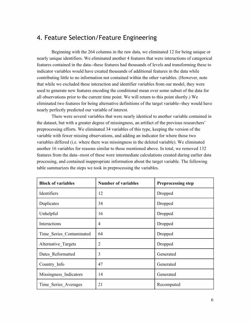
Beginning with the 264 columns in the raw data, we eliminated 12 for being unique or nearly unique identifiers. We eliminated another 4 features that were interactions of categorical features contained in the data­­these features had thousands of levels and transforming these to indicator variables would have created thousands of additional features in the data while contributing little to no information not contained within the other variables. (However, note that while we excluded these interaction and identifier variables from our model, they were used to generate new features encoding the conditional mean over some subset of the data for all observations prior to the current time point. We will return to this point shortly.) We eliminated two features for being alternative definitions of the target variable­­they would have nearly perfectly predicted our variable of interest.

There were several variables that were nearly identical to another variable contained in the dataset, but with a greater degree of missingness, an artifact of the previous researchers’ preprocessing efforts. We eliminated 34 variables of this type, keeping the version of the variable with fewer missing observations, and adding an indicator for where those two variables differed (i.e. where there was missingness in the deleted variable). We eliminated another 16 variables for reasons similar to those mentioned above. In total, we removed 132 features from the data­­most of these were intermediate calculations created during earlier data processing, and contained inappropriate information about the target variable. The following table summarizes the steps we took in preprocessing the variables.

Block of variables Number of variables Preprocessing step

Identifiers 12 Dropped

Duplicates 34 Dropped

Unhelpful 16 Dropped

Interactions 4 Dropped

Time_Series_Contaminated 64 Dropped

Alternative_Targets 2 Dropped

Dates_Reformatted 3 Generated

Country_Info 47 Generated

Missingness_Indicators 14 Generated

Time_Series_Averages 21 Recomputed

6

Categorical 4 Transformed to indicators

Flag_Possible_Error 13 Retained

Target 1 Retained

Binary_Useful 22 Retained

Judge_Demographics 27 Retained

Time_Series_Lags 26 Retained

Other_Potentially_Useful 18 Retained

Total: 132 variables dropped, 64 variables generated, 21 variables replaced, 4 categorical variables transformed to 300 indicator variables. 264 features → 492 features

The raw data contained a set of features which we considered to be a potentially rich source of information: for each observation, the data contained information about the proportion of asylum granted for all other cases in the same court, all other cases decided by the same judge, all other cases decided by the same judge for the same nationality, and so on. All in all, there were 21 features that encoded the conditional mean grant rate over a specific subset of the data. However, these averages were computed over both past and future data, and therefore these features would not be usable in a typical prediction setting. We therefore regenerated these features to average over only those cases which occurred earlier in time to the current case. If a case occurred on the same day as the current case and its order within the day was unknown, we did not include that case in re­computing the average grant rate.

The lag variables, such as the previous decision for that judge, the number of grants for the previous ten cases of that judge, and other time­series data (26 features in total) were already available in the raw data and did not need to be created. However, for two of these features­­the features encoding the judge’s decision in his previous two asylum cases­­there was an exceptionally high rate of missing data. The judge’s previous decision had 54% missing data, and the judge’s second­to­last decision had 77% missing data. This missingness was likely to be an artifact of the way the feature was generated by the previous researchers, so we created a function to fill these values in ourselves with the value of the target variable on the last or second­to­last case for the same judge. For the variant of the target variable we chose to use, there was no missing data (as mentioned previously, there were two available variants of the target variable that were identical but with 17.3% and 13.6% missingness­­here, the missingness indicated that the order of the case within the day was unknown). If the time interval between the current case and the judge’s previous available case was more than 30 days, we did not impute these values from the previous value. We added a feature indicating when each of these values were imputed.

The raw data contained no information about the asylum seeker’s country of origin beyond its name. We obtained data from the Pew Forum and World Bank about the GDP of a

7

country, level of economic development, geographic region and subregion, as well as the proportion of Christians, Muslims, Hindus, Buddhists, Jews, and religiously unaffiliated individuals in a country. (We also obtained year­by­year data on civil wars and ethnic conflicts across all countries, but were unable to merge this data with our asylum seekers’ data.) This step required extensive processing to resolve country names with alternate spellings, country names that changed over time, and countries that entered into or dissolved from existence during the 4 decades spanned by the data. After transforming all categorical data in the country­level information to indicator variables, merging in these features added 47 new variables to the data set. Adding the information about region and subregion, majority religion of a country, and level of economic development, allowed for the possibility of generalizing over groups of countries (e.g. poor countries, East Asian countries, Muslim countries) to uncover potential biases in judges’ decision­making behavior.

5. Missing Data Imputation and Data Partitioning

Of the 478 features in the data, 73 contained some level of missingness. Note that the initial preprocessing steps went a long way towards handling missing data­­prior to preprocessing, 166 out of 264 features contained some missingness, and listwise deletion of all observations containing any missing data would have resulted in throwing away over 87% of the data. The features with missing observations were a mix of time­series lag variables and non­time­series variables, and we dealt with these two types of missing data differently.

After using last observation carried forward in the two lag variables with over 50% missing data (described above), the amount of missing data in those 73 features ranged from 18.6% missing in some of the conditional mean variables to less than 1% missing. The median level of missingness in those variables that had at least one missing value was 5%. All of the demographic information on the judges was merged in from another dataset, and this information was missing for 5% of all cases, which amounted to missing biographical data for 13% of all judges. Listwise deletion of all observations containing any missing data would have resulted in a data set of 312,577 observations, or 62% of the size of the original data. Rather than taking that approach and conducting a complete case analysis, we chose to use mean imputation on the features containing missing data, creating indicator variables where there was missing data. Because some of the patterns of missingness were already encoded in the Flag_Possible_Error variables given in the data, and because the patterns of missingness were overlapping in many variables (for example, there were 18 variables that exactly the same observations missing as the others), we were able to indicate the observations we imputed in a set of 14 missingness indicators. When added to the 478 features in our data following preprocessing and feature generation, the data in our final analysis contained 492 features­­491 predictors and 1 binary target variable.

Since we are primarily interested in whether our model generalized to new judges, we avoided using the out­of­the­box training/test split and cross­validation functions in the sklearn package, in favor of implementing our own data partitioning mechanism that randomly sampled judges and included all of their cases in the training set until the training set reached

8

the desired size. For any given judge, all of their cases were either included in the training set or the test set, and all models were tested exclusively on judges whose previous cases they had not been trained on. In total, there were 426 judges, and an 80/20 split of the data left 328 judges in the training set. Note that no identifiers unique to the judge were included as features, but our model did include information about the judge’s gender, experience, education, and prior record of granting asylum. Thus our model performance will allow us to answer the question of whether we can predict the decision­making for a new judge given that we know some basic information about his past decision­making. We can then investigate this question further by leave­one­judge­out validation, where we cycle through the judges leaving every judge in turn out of the training set, and average our out­of­sample prediction performance on each judge to get a better idea of how our model might perform in practice.

6. Predictive Modeling

6.1. Baseline Model We constructed a baseline model on the post­processing dataset, but excluded the features we generated­­that is, our baseline model did not include the 47 country­level features and 21 conditional means over the judge’s and courts previous cases. In total, our baseline model was trained on 423 predictors and 1 target variable. Our baseline model was a regularized logistic regression with L2 penalty and it achieved an accuracy of 74.6%, and an AUC of .804 on the test set of 103,826 observations.

6.2. Grid Search Validation and Model Comparison Next, we trained various models on the processed dataset and compared their performance on our holdout validation set. We initially provided all available features to the candidate models. All our models were built using the scikit­learn machine learning library.

6.2.1. Decision Tree Classifier In general, many decision trees can be constructed from a given set of attributes. While some of the trees are more accurate than others, finding the optimal tree is computationally infeasible because of the exponential size of the search space and the risk of creating overly­complex trees that may not generalize the dataset well by overfitting the training data. However, various efficient algorithms have been developed to construct a reasonably accurate Decision Tree in a reasonable amount of time. These algorithms usually employ a greedy strategy that grows a decision tree by making a series of locally optimum decisions about which attribute to use for partitioning the data. Out of the 10 hyperparameters provided by the scikit­learn for this supervised learning method, we did grid search on four of them, keeping the rest of parameters to their default values. Set of the hyperparameters chosen were:

9

max_depth: This was one of the obviously most important hyperparameter since overly

complex Decision Tree can overfit the training data and too simple trees can underfit the training data. Different values chosen for this hyperparameter were: 1, 3, 5, 7, 9, 11, 13, 15, 17, 19, 20, 30, 40, 50 and max_depth.

criterion: This parameter was important because it measures the effectiveness of the

split using either ‘Gini impurity’ or ‘Entropy’ as the measure.

splitter: How the dataset was split at each node was important as well. This hypermeter value was chosen to be either ‘best’ or ‘random’. While the former would give best possible split at each node for a given criterion and latter would give best random split at each node for the given criterion, in other words, ‘random’ chooses the threshold randomly instead of optimizing the theta.

min_sam_leaf: Though we later found that restricting the minimum number of samples

required to be in the leaf node did not make much of a difference, we initially choose this hyperparameter to see if there is an improved performance by tuning this parameter.

With grid search on these chosen hyperparameters, we built 180 different decision tree models. We evaluated their performances on the test data and choose the best validated model among these 180 candidate models.

6.2.2. Random Forest Classifier Random Tree classifier was chosen to be our next model in the pipeline because this ensemble method avoid the problem of overfitting and uses averaging of individual tree performances to improve the predictive accuracy, using the out­of­bag prediction error. While building this model using the scikit­learn, we choose the following parameters to tune the model:

max_depth, splitter, criterion, min_sam_leaf: These hyperparameters were chosen for the same reason as given for Decision Tree model. Though we initially thought that tuning the ‘max_depth’ parameter for Random Forest model may not be a good practice, but our later analysis revealed that variations in this parameter value did have some significant difference in the model performance.

n_estimators: This was one of the most important hyperparameter to tune because the number of trees in the forest is generally highly correlated with the model performance.

warm_start: This parameter was chosen to see some differences in the performance by either using or not using the solution of the previous call to fit the ensemble.

With grid search on these chosen hyperparameters, we built 1260 different Random Forest models, choosing the best validated Random Forest model.

10

6.2.3. Adaboost The next ensemble method chosen for our modelling problem was Adaboost with Decision Tree as weak classifier. This method has proven to achieve better generalization property than a single Decision Tree classifier. The only hyper parameter chosen for grid search was the ‘max_depth’ of the weak classifier with 1, 5, 10, 25, 50 and ‘maximum possible depth’ selected as the max_depth values.This gave us 6 different models. We were also interested in trying a not­commonly used model, a hybrid of Random Forest and Adaboost where Adaboost is performed with Random forest as a weak classifier. Though Adaboost algorithm works faster with simple weak learners than with learners that build forests of trees, this combination has advantages including increased prediction ability of the models in some data sets. Our final test performance analysis showed that Adaboost with Random Forest outperformed both the Adaboost with Decision Tree model and the standalone Random forest model.

6.2.4. Loss Functions Based Binary Classifiers Apart from using the tree based classification models for our dataset, we were interested in seeing if there are any better performances with the loss function based classification models. Four different types of loss functions were used: Hinge Loss, Square Hinge Loss, Modified Huber Loss and Log loss.

Hinge loss gave us a linear SVM model. Log loss gave us a logistic regression model.

For each of these models, three different types of regularizations were used: L1, L2 and ElasticNet. Since our dataset has large number of features, we wanted to make use of the feature selection capabilities of L1 and ElasticNet penalties. Our mixture parameter for ElasticNet was .15, biased towards the L1 penalty much more so than L2. Through grid search, we evaluated and compared the performance of all possible combinations of the candidate hyperparameters. Stochastic gradient descent/subgradient descent methods were used to minimize each of these objective functions because they converge much faster than the gradient descent approach and they are capable of achieving state­of­the art performances.

11

7. Model Evaluation Model performances were measured based on the following three evaluation metrics:

Accuracy Score AUC Score ROC Curve

For each classification model, we calculated both the predicted score as well as the

predicted probability. We used the former to compute the Accuracy score for the model, and the latter was used for calculating the AUC score and plotting the ROC curve.

Since the Accuracy score uses a single classification threshold of 0.5, with the probability above 0.5 represented one class and below 0.5 represented the other class, this score may be misleading for imbalanced classes, such as this dataset (our data contained 34.7% decisions to grant asylum, and 65.3% decisions to deny asylum). In contrast, the AUC measures the ability of the model to predict a higher score for positive examples as compared to negative examples. Because it is independent of the score cut­off, we can get a sense of the prediction accuracy of our model from the AUC metric without picking a threshold. And our third metric, ROC curve, which depends on the True Positive Rates and False Positive Rates, was used to visually compare the models.

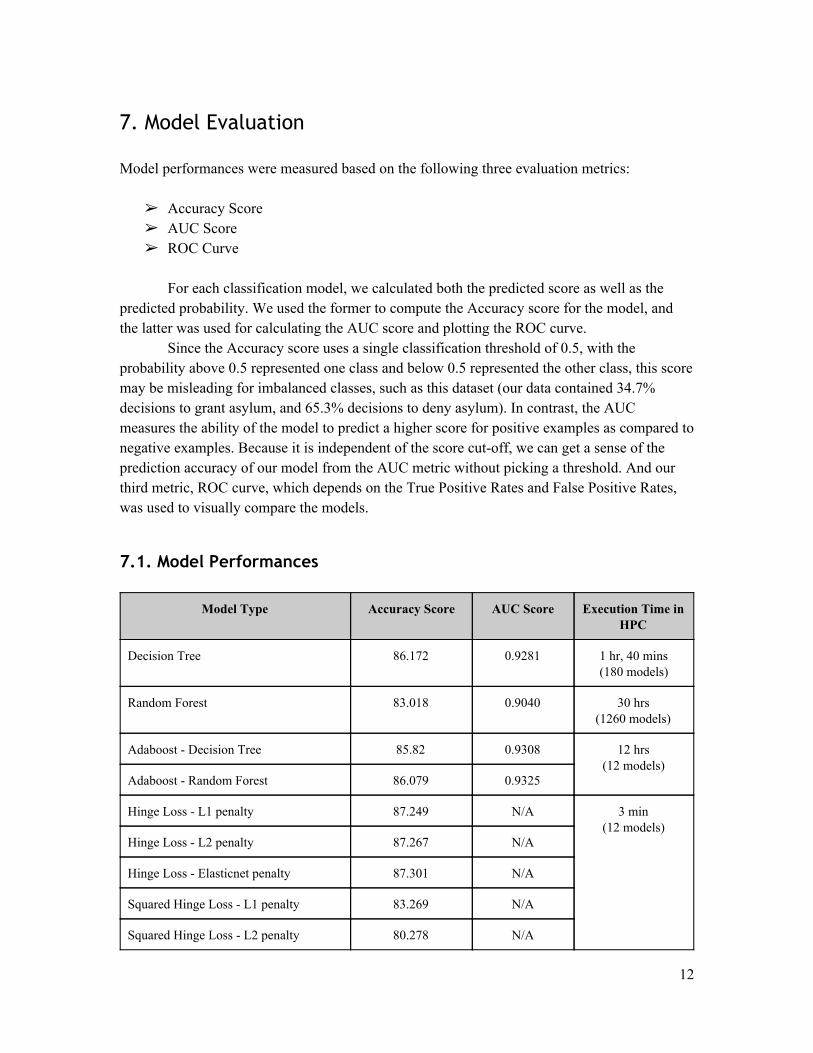
7.1. Model Performances

Model Type Accuracy Score AUC Score Execution Time in HPC

Decision Tree 86.172 0.9281 1 hr, 40 mins (180 models)

Random Forest 83.018

0.9040 30 hrs (1260 models)

Adaboost ­ Decision Tree 85.82 0.9308 12 hrs (12 models)

Adaboost ­ Random Forest 86.079 0.9325

Hinge Loss ­ L1 penalty 87.249 N/A 3 min (12 models)

Hinge Loss ­ L2 penalty 87.267 N/A

Hinge Loss ­ Elasticnet penalty 87.301 N/A

Squared Hinge Loss ­ L1 penalty 83.269 N/A

Squared Hinge Loss ­ L2 penalty 80.278 N/A

12

Squared Hinge Loss ­ Elasticnet penalty 80.209 N/A

Log Loss ­ L1 Penalty 87.140 0.93782

Log Loss ­ L2 Penalty 87.144 0.93788

Log Loss ­Elasticnet Penalty 87.162 0.93588

Modified Huber Loss ­ L1 Penalty 87.538 0.93757

Modified Huber Loss ­ L2 Penalty 87.219 0.93608

Modified Huber Loss ­Elasticnet Penalty 87.177 0.93588

7.2. Accuracy Score Based Model Comparison

Among all our model types, Modified Huber Loss with L1 penalty gave us the best accuracy rate of 87.538% and hence it is the model with lowest test error, which can be seen as the rightmost bar on the above plot . This model is closely followed by linear SVM model(Hinge loss) with Elasticnet penalty with an accuracy rate of 87.301%. Not far behind is the Logistic Regression model(Log Loss) with Elasticnet Penalty having an accuracy rate of 87.162%.

Random forest performed the least among all our models with an accuracy rate of 83.018%.

13

Nevertheless, all our models performed better than an accuracy rate that we would have got by just guessing the majority class in our test data. This majority class guess error rate(which corresponds to an accuracy rate of (100­39.07) = 60.930%) is given by the red line on the above plot.

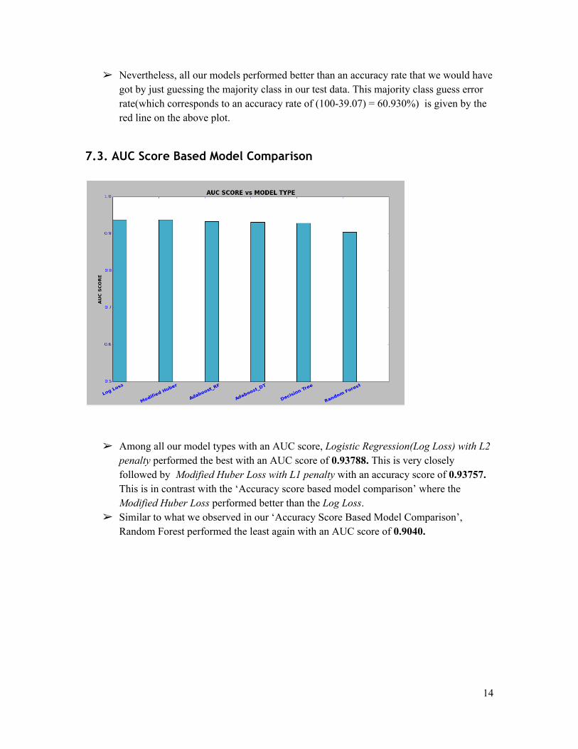
7.3. AUC Score Based Model Comparison

Among all our model types with an AUC score, Logistic Regression(Log Loss) with L2 penalty performed the best with an AUC score of 0.93788. This is very closely followed by Modified Huber Loss with L1 penalty with an accuracy score of 0.93757. This is in contrast with the ‘Accuracy score based model comparison’ where the Modified Huber Loss performed better than the Log Loss.

Similar to what we observed in our ‘Accuracy Score Based Model Comparison’, Random Forest performed the least again with an AUC score of 0.9040.

14

7.4. ROC Curve Based Model Comparison

Among all the max_depth values we chose, max_depth of 5 gave the better predictive power for the decision tree, which can be easily seen by the shape of the ROC curve for this depth. This curve is more towards the TPR(true positive rate) than the others curves plotted for the decision tree.

In case of Random Forest, ROC curve corresponding to max_depth of 7 indicates that this max_depth gave us the better accuracy.

8. Important Features Analysis Because we included a large number of features in our model, we were interested in understanding the types of features that strongly influence the model’s prediction of asylum granting decisions. For each family of models, we selected the validated model with optimal hyperparameter values, and then we averaged the feature importances across all families of high­performing models.

8.1. Feature Score Based analysis sklearn’s feature_importances_ was used to get the set of features for which the corresponding feature value was more than 0. This was done for all the models we built. Scores from all these models were combined to get the final score for each feature and we picked the top 30 features in terms of higher feature values as given below,

15

Among the top 30 important features, the top three features were all related to the average grant rate for the judge’s previous decisions for a specific nationality (including the judge’s previous decisions for that nationality x defensive status combination and the judge’s previous decisions for that nationality in that year). Each of these were strongly positively associated with the target variable (positive coefficients in our models). The more often a judge granted asylum to asylum seekers of a particular nationality in his previous decisions, the more confident our predictions of granting asylum in the current case.

Another class of important features was related to the number of cases where the judge granted asylum out of the previous n asylum cases for that judge. These features had positive coefficients in our models as well­­the more often a judge had granted asylum recently, the more likely the judge would grant asylum again.

Among the country­level features we merged from external data sources, the following three features came up within top 30 features:

the percentage of Muslims in the asylum seeker's country of origin, as well as the percentage of Christians in the asylum seeker's country of origin. Asylum seekers were less likely to be granted asylum if they came from a majority Muslim country, and they were also less likely to be granted asylum if they came from a majority Christian country. The decreased likelihood of asylum from Christian­majority countries is closely related to our next finding, in that the Latin American countries are nearly all Christian­majority countries with a lower than average rate of granting asylum. In general, asylum was less likely

16

to be granted for countries where more than 95% of the population observed the majority religion.

Whether or not the asylum seeker’s originates from the Latin America and Caribbean region. These features had negative coefficients in our model. This is likely due to the fact that this was the region where the largest number of asylum seekers hailed from, and judges may have been enforcing some kind of internal quota on the region­­individuals and families from Latin America comprised 38.8% of all asylum seekers, but only 17.1% of those granted asylum. It is also worth noting that while 48% of all asylum cases were defensive in nature (the asylum seeker applied for asylum when on the verge of deportation), 57.2% of asylum seekers of asylum seekers from the Caribbean applied for asylum from a defensive status.

8.2. Analysis of Information Gain and Loss by Removing Feature Blocks We continued our analysis by removing certain thematically coherent blocks of features from the analysis. We created three different subsets of features to exclude from the data:

Remove all country­level information, including 47 features we generated from outside data and 227 indicator features encoding the specific country of origin.

Number of features remaining: 217 predictors + 1 target Remove all time­series lag data, for a total of 28 features, encoding information about

the judge’s and the court’s most recent asylum decisions Number of features remaining: 463 predictors + 1 target

Remove all time­series lag data as well as all biographical information about the judges (gender, education, experience, etc.). This involved dropping the 28 above­mentioned lag variables as well as dropping the 36 variables previously merged in from the judge­level demographic data. Number of features remaining: 427 predictors + 1 target Note that in this particular set of features, as well as the previous set of features with only the lag variables dropped, we retained the conditional averages over a judge’s previous cases (there were 21 variables of this type), so there was still some time­series information available in the data.

We also created two additional sets of features but did not train models on them: one set of features with only the 36 variables related to the judge’s biographical information (leaving a total of 455 predictors), and another set of features with the 28 time­series lag variables dropped as well as the 21 time­series running averages dropped (leaving a total of 442 predictors)

We then compared the model’s out­of­sample prediction performance to the performance of the same family of models with those features included. Our validated out­of­sample error increased with the removal of these features, but for most models the decrease in performance was very slight (between 0.5 to 4 percent decrease in our performance metrics). Interestingly,

17

however, when we removed biographical information about the judges, performance typically increased about 1.1 to 3.4 percent. This indicates that while the relationships between a judge’s previous asylum granting record and current decision­making generalizes well to new judges, the relationship between a judge’s basic biographical information and his decision­making does not generalize well, and associations uncovered by the model in the training set are often reversed or weakened in the test set.

Note that we should not be overly surprised by the very small increase in the test error rate, even after dropping so many features­­our finding can as be explained by the previous section, ‘Feature score based analysis’ which shows that the most important features were the conditional running averages for a particular judge in previous similar cases. These conditional running averages features were not dropped in any of the three alternate sets of features we modeled in this section.

9. Judge Bias Analysis

A major goal of our analysis was to apply the predictive models developed above to measure the generalization performance of our model on each judge, and rank the judges by how far they deviated from typical decision­making behavior, accounting for the possibility that a judge might simply have an unusual case load. To do this, we implemented a method of leave­one­judge­out validation, as follows: For every judge in the data:

1. Fit a model to the data from all judges except judge X 2. Use the model to predict asylum decisions for judge X 3. Evaluate a performance metric on the confusion matrix of predicted versus observed

decisions for judge X For simplicity, we trained these with two types of classifiers: AdaBoost with decision tree stumps and L2­penalized logistic loss, using the best­performing models from our previous predictive modeling analysis.

There are a total of 426 judges in the data, with a median of 819 cases and a mean of 1258 cases seen per judge . For each of the two types of classifiers mentioned above, we computed a confusion matrix for the predictions of the model trained on all other judges and tested on the remaining judge. Performance of the two families of classifiers was very similar, so we will focus our analysis on the Adaboost classifier. Overall generalization performance was good, with a median error rate of 10.6% in the Adaboost classifier and a median F1 score of .815. We threw out the predictions for judges where the number of observed or expected grant decisions was less than 5, as these judges typically had too few or too unbalanced cases to draw reasonable predictions from. This left us with data from 397 judges (29 judges were dropped). Some of these “pathological” judges are worth exploring further­­out of the 15 dropped judges who presided over more than 15 cases, the average grant rate was 6% (compared to the overall grant rate per judge of 30%), so these judges simply didn’t have enough data in each class to explore properly.

18

As a comprehensive and balanced performance metric, we chose to use the phi coefficient (also known as the Matthew’s correlation coefficient), a measure of the association between the observed and predicted decisions. We selected this because it tends to be a balanced performance metric even when the classes are of very different sizes, and because it standardizes over the number of observations. This was critical, because after dropping the 29 judges mentioned above, the number of cases seen by each judge ranged from 13 cases to over 7,000 cases, and the typical class imbalance was 30/70, but it ranged from 3% positive cases to 89.7% positive. A coefficient of +1 represents a perfect prediction model, 0 an average random prediction and ­1 a perfect inverse prediction. The mean phi coefficient was 0.695, indicating that, on average, most of the judges’ predicted behavior was very closely correlated with their actual behavior. The phi coefficients for all 397 judges ranged from .22 to 1.0.

We then ranked the judges in order of the weakest association between predicted and observed outcomes. Out of the top ten most poorly predicted judges in our dataset (the top six are annotated in the plots below), there was diversity in their number of cases seen and proportion of asylum decisions granted, so there was no overly facile explanation for why the model predicted these judges so poorly: 3 of the 10 were in the lowest quartile for proportion of asylum cases granted, 2 were in the second quartile, 1 was in the third quartile, and 4 were in the highest quartile for proportion granted. For the number of cases seen, 2 of these outliers fell into the lowest quartile, 4 fell in the second quartile, 1 judge fell in the third quartile, and 2 were in the highest quartile for number of cases seen. So importantly, our model isn’t just failing on the judges with the fewest cases, or the judges with the highest (or lowest) proportion of cases granted. In the plots below, we can see that where our model failed, it was typically a case of too many false negatives­­we underestimated the number of times they would grant asylum (notice that all of our top 6 outliers lie below the trend line).

We compared the average values of each of our outlier judges to the average values of the features which were ranked as most important in our feature analysis. It was challenging to find a single answer that accounted for all of the judges’ status as outliers, but for some of the judges, we were able to draw some tentative explanations that need further evaluation. The most poorly fit judge in our data, for example, decided most of his cases in 1990, and nearly 84% of the asylum seekers in his cases came from Latin America or the Caribbean, with only

19

7% of of the asylum from China. In fact, the time period of the data was the most likely explanation for the difficulty fitting particular judges­­using the leave­one­judge­out validation model as we implemented it, it was possible for the model to be trained on data that was substantially separated in time from the test set. Of the top ten outliers we identified, 5 had careers that mainly spanned the earliest 10 percent of the data, and 3 had careers that spanned the latest 10 percent of the data. With this in mind, it is surprising that overall, our prediction performance did relatively well, but we could greatly improve performance by limiting our training set for each judge to the cases of all other judges that occurred within one year of the cases for the judge we wish to make predictions on.

10. Limitations in our Analysis

10.1. Limitations due to unavailable features

Asylum cases should have a strong reason for seeking asylum in the US. At the time of seeking asylum, if the asylum seeker’s country of origin was affected by any internal conflict or war between different ethnic groups, then this specific refugee has a strong reason for seeking asylum on the ground that he/she is afraid to return. We believe this information for each country and for each year would have been a very strong feature for our models. Though we obtained year­by­year, country­by­country information on ethnic conflict, it was impossible to efficiently merge it with the asylum dataset.

Another important feature which was missing from our dataset was the religious background of each refugee. This feature may have had a strong influence in the decision making process for certain judges who were biased towards certain religion or for certain cases where this information was relevant. For example, a review of the many claims for asylum that are granted to refugees from China, the number one country of origin for asylum seekers in our data, indicates that many of these asylum seekers claimed that they were persecuted or feared persecution because of their religion. This includes self­professed Christians and people who attend “underground” churches not registered with the government of China as well as Uighur Muslims and Tibetan Buddhists. While we have added data about the majority religion of an asylum seeker’s country of origin, it would be helpful to see the proportional representation of the asylum seeker’s religion as an added feature­­immigration judges may be more likely to grant asylum to individuals where the asylum seeker’s religion comprises less than 0.5% of of the origin population . In the case of a much smaller country, Sri Lanka, underwent 25 years of civil war from 1983­2009, and the minority Tamils, who are mainly Hindus, fled the country due to fear of prosecution by the majority Sinhalese government, who are mainly Buddhist. Hence, knowing the religious background of these individuals, as well as year­to­year data on the level of ethnic conflict and civil war in a particular country, will help in building a better prediction model.

20

Educational background of the asylum seeker can be an important feature. A refugee with a good education may be viewed as someone who is seeking asylum for economic benefits rather than for a “credible fear”; alternatively, a highly educated asylum seeker may be viewed as someone who can be beneficial to the country. Also, people who speak English well may be more likely to succeed in their cases.

Gender of the asylum seeker is yet another important factor which was missing from our data. Journal of Refugee Studies (see “References”) found that within the cases studied, women were statistically less likely to be granted asylum. Of all the factors studied (except possibly religion) by the author of this journal, gender was the most significant “unobservable factor” that determined the outcome in an asylum seeker’s case. It was hypothesized that women may not be seen as viable threats to government.

According to the United States Citizenship and Immigration Services, the most important determinant of whether asylum is granted is actually whether the asylum seeker complied with all filing deadlines.

A 2000 study suggested that single people were less likely to gain asylum in the United States, presumably because decision makers view them as likely economic migrants. However, whenever an asylum applicant lists numerous young children on their application, Judge may be more hesitant to grant asylum, knowing that the grantee’s entire family will be “following to join” him/her in the United States. Though this may not be the ‘the most’ important factor, marital status of a refugee could have added some predictability in our model if our dataset had it.

10.2. Potentially Insightful Analyses We Did Not Include

As mentioned previously, we ran comparisons of the model with the full set of features available to the model with both the lag variables as well as the judge biographical information removed. Our findings indicated that performance decreased when we removed only the lag variables, but improved again when we removed both the lag variables and the judge information. This suggests that performance may be even stronger if we retained the lag variables but removed only the judge information; however, we did not obtain the predictions from training this model.

Additionally, because the running averages of a judge’s previous decision for a particular nationality were among the most informative features in our model, we might gain additional insight by calculating the running averages of a judge’s decisions for a particular region or subregion, rather than limiting to a single country. For example, there may not be much difference between a judge’s decision­making for asylum seekers from Honduras compared to El Salvador, and collapsing these categories in the conditional mean computations may provide new information. Furthermore, since we did not analyze the information lost by the model by dropping these particular features (we only dropped the lag­recency variables), it would help to compare the performance of the model with and without these features.

Finally, it would be helpful to redo the leave­one­judge­out anomaly detection in a way that respects the time­ordered nature of the training data. Training on data that spans from 1971

21

to 2013 turns out, not surprisingly, to make very poor predictions for the decision behavior of a judge in 2012. Because the career of a particular judge is often fairly constrained in time (compared to the careers of approximately 100 judges included in the test set for the main predictive model we built), fitting the training data may uncover relationships which no longer hold true at the time of a particular judge’s career.

11. Conclusion and Future Work

Overall, we are able to achieve good performance. The strength of our predictive performance does raise potential concerns about whether there is any data leakage. We combed through each of the raw features one by one in order to better understand the most important features in our models and remove all features which contained inappropriate direct knowledge of the target variable. We also split the data into validation sets stratified by judge, both to gauge our generalization performance and to allow our model to learn more general relationships between past and current decision­making.

The most predictive features were those related to the judge’s past decision­making in the judge’s most recent cases as well as in the previous cases featuring an asylum seeker of the same nationality. This indicates that country of origin is extremely important in asylum decisions, but that certain judges may have implicit biases—country of origin is not interpreted the same by every judge. On average, however, asylum seekers from China were much more likely to be granted asylum, and asylum seekers from Latin America as well as from the Middle East/North Africa were much less likely to be granted asylum. Asylum seekers from Muslim countries outside the Middle East/North Africa, including Indonesia, Pakistan, Afghanistan, and Iran, were more likely to be granted asylum than Muslim refugees from the Middle East.

There is not much difference in performance from one model family to another, as long as we have used grid search to validate the hyper­parameters, and validated performance on new judges. However, computation time is a real limiting factor here, and we can achieve the best trade­off between computation time and model performance by choosing the fastest­performing algorithms (e.g. linear SVM or regularized logistic loss with stochastic gradient descent algorithm). In many cases, we were not able to complete all planned analyses because there was not enough time to run the full model, and the stochastic gradient descent algorithms became more convenient to use.

Overall, we are able to generalize well to new judges. We can predict a judge’s decision without explicitly training on that judge if we are told the results of the judge’s previous asylum cases and if the training data spans a similar time frame as the career of the judge we wish to make predictions for. Further investigation is needed to gauge our ability to detect outliers who do not have an unusually high or low rate of granting asylum and whose models have been trained on recent cases only.

22

12. Acknowledgements This project consumed a great amount of work, research and dedication. Still, implementation would not have been possible if we did not have the support of many individuals. Therefore we would like to extend our sincere gratitude to all of them. We would like to thank Daniel Chen for his support in providing and helping us to better understand the data, Gideon Mann for providing the necessary guidance and many helpful suggestions along the way, particularly concerning our anomaly detection methods, and finally, our professor David Rosenberg for introducing each of these algorithms to us and providing us with the foundational knowledge needed to complete this undertaking.

13. References

Keith & Holmes. (2009). A Rare Examination of Typically Unobservable Factors in US Asylum Decisions

UNHCR Population Statistics, 2000­2013. Pew Forum (2012). The Global Religious Landscape: Religious Composition by

Country. World Bank. (2015). The World DataBank: World Development Indicators.

23