genie: a new, fast, and outlier-resistant hierarchical ... · genie: a new, fast, and...

Genie: A new, fast, and outlier-resistanthierarchical clustering algorithm

Marek Gagolewskia,b,∗, Maciej Bartoszukb,c, Anna Cenaa,c

aSystems Research Institute, Polish Academy of Sciencesul. Newelska 6, 01-447 Warsaw, Poland

bFaculty of Mathematics and Information Science, Warsaw University of Technologyul. Koszykowa 75, 00-662 Warsaw, Poland

cInternational PhD Studies Program,Institute of Computer Science, Polish Academy of Sciences

Abstract

The time needed to apply a hierarchical clustering algorithm is most often dominated by the num-ber of computations of a pairwise dissimilarity measure. Such a constraint, for larger data sets, putsat a disadvantage the use of all the classical linkage criteria but the single linkage one. However, itis known that the single linkage clustering algorithm is very sensitive to outliers, produces highlyskewed dendrograms, and therefore usually does not reflect the true underlying data structure –unless the clusters are well-separated. To overcome its limitations, we propose a new hierarchicalclustering linkage criterion called Genie. Namely, our algorithm links two clusters in such a waythat a chosen economic inequity measure (e.g., the Gini- or Bonferroni-index) of the cluster sizesdoes not increase drastically above a given threshold. The presented benchmarks indicate a highpractical usefulness of the introduced method: it most often outperforms the Ward or average link-age in terms of the clustering quality while retaining the single linkage speed. The Genie algorithmis easily parallelizable and thus may be run on multiple threads to speed up its execution further on.Its memory overhead is small: there is no need to precompute the complete distance matrix to per-form the computations in order to obtain a desired clustering. It can be applied on arbitrary spacesequipped with a dissimilarity measure, e.g., on real vectors, DNA or protein sequences, images,rankings, informetric data, etc. A reference implementation of the algorithm has been included inthe open source genie package for R.Please cite this paper as: Gagolewski M., Bartoszuk M., Cena A., Genie: A new, fast, and outlier-resistanthierarchical clustering algorithm, Information Sciences 363, 2016, pp. 8–23, doi:10.1016/j.ins.2016.05.003.

Keywords: hierarchical clustering, single linkage, inequity measures, Gini-index

∗Corresponding author; Email: [email protected]; Tel: +48 22 3810 378; Fax: +48 22 3810 105

Preprint submitted to Information Sciences May 30, 2016

Please cite this paper as: Gagolewski M., Bartoszuk M., Cena A., Genie: A new, fast, and outlier-resistanthierarchical clustering algorithm, Information Sciences 363, 2016, pp. 8–23, doi:10.1016/j.ins.2016.05.003.

1. Introduction

Cluster analysis, compare [31], is one of the most commonly applied unsupervisedmachine learning techniques. Its aim is to automatically discover an underlying structureof a given data set X = x(1), x(2), . . . , x(n) in a form of a partition of its elements: disjointand nonempty subsets are determined in such a way that observations within each groupare “similar” and entities in distinct clusters “differ” as much as possible from each other.This contribution focuses on classical hierarchical clustering algorithms [10, 14] whichdetermine a sequence of nested partitions, i.e., a whole hierarchy of data set subdivisionsthat may be cut at an arbitrary level and may be computed based on a pairwise dissimilaritymeasure d : X × X → [0,∞] that fulfills very mild assumptions: (a) d is symmetric,i.e., d(x, y) = d(y, x) and (b) (x = y) =⇒ d(x, y) = 0 for any x, y ∈ X. This groupof clustering methods is often opposed to – among others – partitional schemes whichrequire the number of output clusters to be set up in advance: these include the k-means, k-medians, k-modes, or k-medoids algorithms [34, 40, 56, 59] and fuzzy clustering schemes[6, 46–48], or the BIRCH (balanced iterative reducing and clustering using hierarchies)method [60] that works on real-valued vectors only.

In the large and big data era, one often is faced with the need to cluster data sets ofconsiderable sizes, compare, e.g., [30]. If the (X, d) space is “complex”, we observe thatthe run-times of hierarchical clustering algorithms are dominated by the cost of pairwisedistance (dissimilarity measure) computations. This is the case of, e.g., DNA sequencesor ranking clustering, where elements in X are encoded as integer vectors, often of con-siderable lengths. Here, one often relies on such computationally demanding metrics asthe Levenshtein or the Kendall one. Similar issues appear in numerous other applicationdomains, like pattern recognition, knowledge discovery, image processing, bibliometrics,complex networks, text mining, or error correction, compare [10, 15, 16, 18, 29].

In order to achieve greater speed-up, most hierarchical clustering algorithms are ap-plied on a precomputed distance matrix, (di, j)i< j, di, j = d(x(i), x( j)), so as to avoid deter-mining the dissimilarity measure for each unique (unordered) pair more than once. This,however, drastically limits the size of an input data set that may be processed. Assumingthat di, j is represented with the 64-bit floating-point (IEEE double precision) type, alreadythe case of n = 100,000 objects is way beyond the limits of personal computers popularnowadays: the sole distance matrix would occupy ca. 40GB of available RAM. Thus, for“complex” data domains, we must require that the number of calls to d is kept as small aspossible. This practically disqualifies all popular hierarchical clustering approaches otherthan the single linkage criterion, for which there is a fast O(n2)-time and O(n)-space al-gorithm, see [41, 42, 56], that requires each di, j, i < j, to be computed exactly once, i.e.,there are precisely (n2 − n)/2 total calls to d.

Nevertheless, the single linkage criterion is not eagerly used by practitioners. This is

2


because it is highly sensitive to observations laying far away from clusters’ boundaries(e.g., outliers). Because of that, it tends to produce highly skewed dendrograms: at itshigher levels one often finds a single large cluster and a number of singletons.

In order to overcome the limitations of the single linkage scheme, in this paper wepropose a new linkage criterion called Genie. It not only produces high-quality outputs(as compared, e.g., to the Ward and average linkage criteria) but is also relatively fast tocompute. The contribution is set out as follows. In the next section, we review some basicproperties of hierarchical clustering algorithms and introduce the notion of an inequityindex, which can be used to compare some aspects of the quality of clusterings obtainedby means of different algorithms. The new linkage criterion, together with its evaluation ondiverse benchmark sets, is introduced in Section 3. In Section 4 we propose an algorithm tocompute the introduced clustering scheme and test its time performance. Please note thata reference implementation of the Genie method has been included in the genie packagefor R [52]. Finally, Section 5 concludes the paper and provides future research directions.

2. A discussion on classical linkage criteria

While a hierarchical clustering algorithm is being computed on a given data set X =

x(1), x(2), . . . , x(n), there are n− j clusters at the j-th step of the procedure, j = 0, . . . , n−1.It is always true that C( j) = C( j)

1 , . . . ,C( j)n− j with C( j)

u ∩ C( j)v = ∅ for u , v, C( j)

u , ∅, and⋃n− ju=1 C( j)

u = X. That is, C( j) is a partition of X.Initially, we have that C(0) = x(1), . . . , x(n), i.e., C(0)

i = x(i), i = 1, . . . , n. In otherwords, each observation is the sole member of its own cluster. When proceeding fromstep j− 1 to j, the clustering procedure decides which of the two clusters C( j−1)

u and C( j−1)v ,

u < v, are to be merged so that we get C( j)i = C( j−1)

i for u , i < v, C( j)u = C( j−1)

u ∪C( j−1)v , and

C( j)i = C( j−1)

i+1 for i > v. In the single (minimum) linkage scheme, u and v are such that:

arg min(u,v),u<v

(min

a∈C( j−1)u ,b∈C( j−1)

v

d(a,b)).

On the other hand, the complete (maximum) linkage is based on:

arg min(u,v),u<v

maxa∈C( j−1)

u ,b∈C( j−1)v

d(a,b) ,

the average linkage on:

arg min(u,v),u<v

1

|C( j−1)u ||C( j−1)

v |

∑a∈C( j−1)

u ,b∈C( j−1)v

d(a,b)

,3


and Ward’s (minimum variance) method, compare [41] and also [44], on:

arg min(u,v),u<v

1

|C( j−1)u | + |C( j−1)

v |×

×

( ∑a∈C( j−1)

u ,b∈C( j−1)v

2d2(a,b) −|C( j−1)

v |

|C( j−1)u |

∑a,a′∈C( j−1)

u

d2(a, a′) −

|C( j−1)u |

|C( j−1)v |

∑b,b′∈C( j−1)

v

d2(b,b′)

),

where d is a chosen dissimilarity measure.

2.1. Advantages of single-linkage clusteringThe main advantage behind the single linkage clustering lies in the fact that its most

computationally demanding part deals with solving the minimum spanning tree (MST,see [27]) problem, compare, e.g., the classical Prim’s [51] or Kruskal’s [37] algorithmsas well as a comprehensive historical overview by Graham and Hell [28]. In particular,there is an algorithm [45] which can be run in parallel and which requires exactly (n2 −

n)/2 distance computations. Moreover, under certain assumptions on d (e.g., the triangleinequality) and the space dimensionality, the Kruskal algorithm may be modified so as tomake use of some nearest-neighbor (NN) search data structure which enables to speed upits computations further on (the algorithm can also be run in parallel). Having obtainedthe MST, a single linkage clustering may then be computed very easily, compare [54].

For the other three mentioned linkage schemes there is, e.g., a quite general nearest-neighbor chains algorithm [43], as well as some other methods which require that, e.g.,X is a subset of the Euclidean space Rd, see [41, 42] for a survey. Unfortunately, weobserve that all these algorithms tend to quite frequently refer to already computed dis-similarities; it may be shown that they use up to 3n2 distance computations. Practically,the only way to increase the performance of these algorithms [45] is to pre-compute thewhole distance matrix (more precisely, the elements either above or below its diagonal).However, we already noted that such an approach is unusable for n already of moderateorder of magnitude (“large data”).

2.2. Drawbacks of single-linkage clusteringNevertheless, it may be observed that unless the underlying clusters are very well-

separated, the single linkage approach tends to construct clusters of unbalanced sizes, oftenresulting – at some fixed dendrogram cut level – in a single large cluster and a number ofsingletons or ones with a very low cardinality.

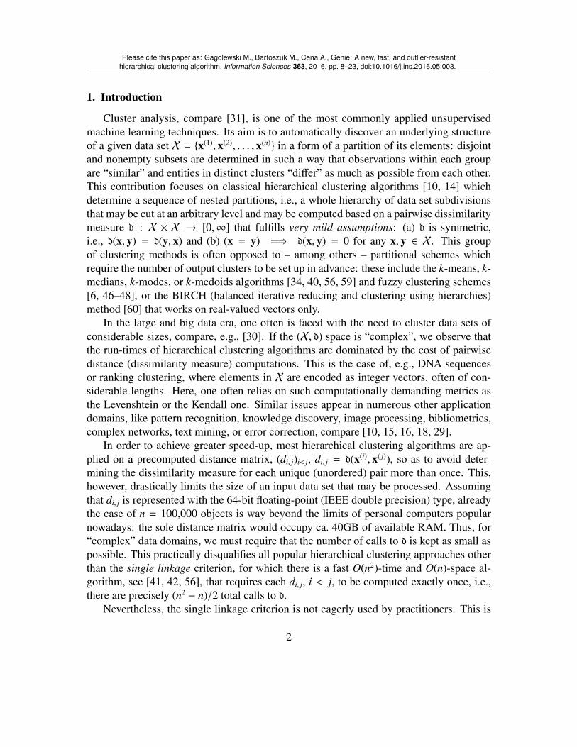
For instance, Figure 1 depicts a dendrogram resulting in applying the single linkageclustering on the famous Fisher’s Iris data set [19] (available in the R [52] datasets pack-age, object name iris) with respect to the Euclidean distance. At the highest level, there

4


0.0

0.5

1.0

1.5

Hei

ght

Figure 1: Dendrogram for the single linkage clustering of the Iris data set.

are two clusters (50 observations corresponding to iris setosa and 100 both to virginica andversicolor) – these two point groups are well-separated on a 4-dimensional plane. Here,high skewness may be observed in the two subtrees, e.g., cutting the left subtree at theheight of 0.4 gives us a partition consisting of three singletons and one large cluster of size47. These three observations lay slightly further away from the rest of the points. Whenthe h = 0.4 cut of the whole tree is considered, there are sixteen singletons, three clustersof size 2, one cluster of size 4, and three large clusters of sizes 38, 39, and 47 (23 clustersin total).

In order to quantitatively capture the mentioned dendrogram skewness, we may referto the definition of an inequity (economic inequality, poverty) index, compare [2, 8, 24]and, e.g., [35, 36] for a different setting.

Definition 1. For a fixed n ∈ N, let G denote the set of all non-increasingly ordered n-tuples with elements in the set of non-negative integers, i.e., G = (x1, . . . , xn) ∈ Nn

0 : x1 ≥

· · · ≥ xn. Then F : G → [0, 1] is an inequity index, whenever:

(a) it is Schur-convex, i.e., for any x, y ∈ G such that∑n

i=1 xi =∑n

i=1 yi, if it holds for alli = 1, . . . , n that

∑ij=1 x j ≤

∑ij=1 y j, then F(x) ≤ F(y),

(b) infx∈G F(x) = 0,

(c) supx∈G F(x) = 1.

5


Notice that, under the current assumptions, if we restrict ourselves to the set of se-quences with elements summing up to n, the upper bound (meaning complete inequality)of each inequity index is obtained for (n, 0, 0, . . . , 0) and the lower bound (no inequality)for the (1, 1, 1, . . . , 1) vector.

Every inequity index like F fulfills a crucial property called the Pigou-Dalton principle(also known as progressive transfers). Namely, for any x ∈ G, i < j, and h > 0 such thatxi − h ≥ xi+1 and x j−1 ≥ x j + h, it holds that:

F(x1, . . . , xi, . . . , x j, . . . , xn) ≥ F(x1, . . . , xi − h, . . . , x j + h, . . . , xn).

In other words, any income transfer from a richer to a poorer entity never increases thelevel of inequity. Notably, such measures of inequality of wealth distribution are not onlyof interest in economics: it turns out, see [3, 4], that they can be related to ecologicalindices of evenness [49], which aim to capture how evenly species’ populations are dis-tributed over a geographical region, compare [11, 32, 50] or measures of data spread [23].

Among notable examples of inequity measures we may find the normalized Gini-index[25]:

G(x) =

∑n−1i=1

∑nj=i+1 |xi − x j|

(n − 1)∑n

i=1 xi(1)

or the normalized Bonferroni-index [7]:

B(x) =n

n − 1

1 − ∑ni=1

1n−i+1

∑nj=i x j∑n

i=1 xi

. (2)

Referring back to the above motivational example, we may say that there is often a highinequality between cluster sizes in the case of the single linkage method. Denoting by ci =

|C( j)i | the size of the i-th cluster at the j-th iteration of the algorithm, F(c(n− j), . . . , c(1)) tends

to be very high (here c(i) denotes the i-th smallest value in the given sequence, obviouslywe always have

∑ni=1 ci = n.).

Figure 2 depicts the Gini-indices of the cluster size distributions as a function of thenumber of clusters in the case of the Iris data set and the Euclidean distance. The outputsof four clustering methods are included: single, average, complete, and Ward linkage.The highest inequality is of course observed in the case of the single linkage algorithm.For instance, if the dendrogram is cut at height of 0.4 (23 clusters in total, their sizes areprovided above), the Gini-index is as high as ' 0.76 (the maximum, 0.85, is obtainedfor 10 clusters). In this example, the Ward method keeps the Gini-index relatively low.Similar behavior of hierarchical clustering algorithms may be observed for other data sets.

6


Number of clusters

Gin

i ind

ex (

clus

ter

size

s)

0.0

0.2

0.4

0.6

0.8

1.0

10 30 50 70 90 110 130 150

singlecompleteaverageWard

Figure 2: The Gini-indices of the cluster size distributions in the case of the Iris data set: single, average,complete, and Ward linkage.

3. The Genie algorithm and its evaluation

3.1. New linkage criterionIn order to compensate the drawbacks of the single linkage scheme, while retaining its

simplicity, we propose the following linkage criterion which from now on we refer to asthe Genie algorithm. Let F be a fixed inequity measure (e.g., the Gini-index) and g ∈ (0, 1]be some threshold. At step j:

1. if F(c(n− j), . . . , c(1)) ≤ g, ci = |C( j)i |, apply the original single linkage criterion:

arg min(u,v),u<v

(min

a∈C( j)u ,b∈C( j)

v

d(a,b)),

2. otherwise, i.e., if F(c(n− j), . . . , c(1)) > g, restrict the search domain only to pairs ofclusters such that one of them is of the smallest size:

arg min(u,v),u<v,

|C( j)u |=mini |C

( j)i | or

|C( j)v |=mini |C

( j)i |

(min

a∈C( j)u ,b∈C( j)

v

d(a,b)).

7


This modification prevents drastic increases of the chosen inequity measure and forcesearly merges of small clusters with some other ones. Figure 3 gives the cluster size distri-bution (compare Figure 2) in case of the proposed algorithm and the Iris data set. Here, weused four different thresholds for the Gini-index, namely, 0.3, 0.4, 0.5, and 0.6. Of course,whatever the choice of the inequity index, if g = 1, then we obtain the single linkagescheme.

Number of clusters

Gin

i ind

ex (

clus

ter

size

s)

0.0

0.2

0.4

0.6

0.8

1.0

10 30 50 70 90 110 130 150

gini_0.3gini_0.4gini_0.5gini_0.6

Figure 3: The Gini-indices of the cluster size distributions in the case of the Iris data set: the Genie algorithm;the Gini-index thresholds are set to 0.3, 0.4, 0.5, and 0.6.

On a side note, let us point out a small issue that may affect the way the dendrogramsresulting in applying the Genie algorithm are plotted. As now the “heights” at whichclusters are merged are not being output in a nondecreasing order, they should somehow beadjusted when drawing such diagrams. Yet, the so-called reversals (inversions, departuresfrom ultrametricity) are a well-known phenomenon, see [39], and may also occur in otherlinkages too (e.g., the nearest-centroid one).

3.2. Benchmark data sets descriptionIn order to evaluate the proposed Genie linkage scheme, we shall test it in various

spaces (points in Rd for some d, images, character strings, etc.), on balanced and unbal-anced data of different shapes. Below we describe the 29 benchmark data sets used, 21of which are in the Euclidean space and the remaining 8 ones are non-Euclidean. Allof them are available for download and inspection at http://www.gagolewski.com/

8

http://www.gagolewski.com/resources/data/clustering/



resources/data/clustering/. Please notice that most of the data sets have alreadybeen used in the literature for verifying the performance of various other algorithms.

In each case below, n denotes the number of objects and d – the space dimensionality(if applicable). For every data set its author(s) provided a vector of true (reference) clusterlabels. Therefore, we below denote with k the true number of underlying clusters (resultingdendrograms should be cut at this very level during the tests). Moreover, we include theinformation on whether the reference clusters are of balanced sizes. If this is not the case,the Gini-index of cluster sizes is reported.

Character strings.

• actg1 (n = 2500, mean string length d = 99.9, k = 20, balanced), actg2 (n = 2500,mean d = 199.9, k = 5, the Gini-index of the reference cluster sizes is equal to0.427), actg3 (n = 2500, mean d = 250.2, k = 10, Gini-index 0.429) – charac-ter strings (of varying lengths) over the a, c, t, g alphabet. First, k random strings(of identical lengths) were generated for the purpose of being cluster centers. Eachstring in the data set was created by selecting a random cluster center and thenperforming many Levenshtein edit operations (character insertions, deletions, sub-stitutions) at randomly chosen positions. For use with the Levenshtein distance.

• binstr1 (n = 2500, d = 100, k = 25, balanced), binstr2 (n = 2500, d = 200, k =

5, Gini-index 0.432), binstr3 (n = 2500, d = 250, k = 10, Gini-index 0.379)– character strings (each of the same length d) over the 0,1 alphabet. First, krandom strings were generated for the purpose of being cluster centers. Each stringin the data set was created by selecting a random cluster center and then modifyingits digits at randomly chosen positions. For use with the Hamming distance.

Images. These are the first 2000 digits from the famous MNIST database of handwrit-ten digits by Y. LeCun et al., see http://yann.lecun.com/exdb/mnist/; clusters areapproximately balanced.

• digits2k_pixels (d = 28 × 28, n = 2000, k = 10) – data consist of 28 × 28pixel images. For testing purposes, we use the Hamming distance on correspondingmonochrome pixels (color value is marked with 1 if the gray level is in the (32, 255]interval and 0 otherwise).

• digits2k_points (d = 2, n = 2000, k = 10) – based on the above data set, werepresent the contour of each digit as a set of points in R2. Brightness cutoff of 64was used to generate the data. Each digit was shifted, scaled, and rotated if needed.For testing, we use the Hausdorff (Euclidean-based) distance.

9



http://yann.lecun.com/exdb/mnist/


SIPU benchmark data sets. Researchers from the Speech and Image Processing Unit,School of Computing, University of Eastern Finland prepared a list of exemplary bench-marks, which is available at http://cs.joensuu.fi/sipu/datasets/. The data setshave already been used in a number of papers. Because of the problems with computingthe other linkages in R as well as in Python, see the next section for discussion, we choseonly the data sets of sizes ≤ 10000. Moreover, we omitted the cases in which all the al-gorithms worked flawlessly, meaning that the underlying clusters were separated too well.In all the cases, we rely on the Euclidean distance.

• s1 (n = 5000, d = 2, k = 15), s2 (n = 5000, d = 2, k = 15), s3 (n = 5000, d = 2, k =

15), s4 (n = 5000, d = 2, k = 15) – S-sets [21]. Reference clusters are more or lessbalanced.

• a1 (n = 3000, d = 2, k = 20), a2 (n = 5250, d = 2, k = 35), a3 (n = 7500, d = 2, k =

50) – A-sets [38]. Classes are fully balanced.• g2-2-100 (n = 2048, d = 2, k = 2), g2-16-100 (n = 2048, d = 16, k = 2),g2-64-100 (n = 2048, d = 64, k = 2) – G2-sets. Gaussian clusters of varyingdimensions, high variance. Clusters are fully balanced.

• unbalance (n = 6500, d = 2, k = 8). Unbalanced clusters, the Gini-index of refer-ence cluster sizes is 0.626.

• Aggregation (n = 788, d = 2, k = 7) [26]. Gini-index 0.454.• Compound (n = 399, d = 2, k = 6) [58]. Gini-index 0.440.• pathbased (n = 300, d = 2, k = 3) [12]. Clusters are more or less balanced.• spiral (n = 312, d = 2, k = 3) [12]. Clusters are more or less balanced.• D31 (n = 3100, d = 2, k = 31) [55]. Clusters are fully balanced.• R15 (n = 600, d = 2, k = 15) [55]. Clusters are fully balanced.• flame (n = 240, d = 2, k = 2) [22]. Gini-index 0.275.• jain (n = 373, d = 2, k = 2) [33]. Gini-index 0.480.

Iris. The Fisher’s Iris [19] data set, available in the R [52] datasets package. Again, theEuclidean distance is used.

• iris (d = 4, n = 150, k = 3) – the original data set. Fully balanced clusters.• iris5 (d = 4, n = 105, k = 3) – an unbalanced version of the above one, in which

we took only five last observations from the first group (iris setosa). Gini-index0.429.

3.3. Benchmark resultsIn order to quantify the degree of agreement between two k-partitions of a given set,

the notion of the FM-index [20] is very often used.

10

http://cs.joensuu.fi/sipu/datasets/


Definition 2. Let C = C1, . . . ,Ck and C′ = C′1, . . . ,C′k be two k-partitions of the set

x(1), . . . , x(n). The Fowlkes-Mallows (FM) index is given by:

FM-index(C,C′) =

∑ki=1

∑kj=1 m2

i, j − n√(∑ki=1

(∑kj=1 mi, j

)2− n

) (∑kj=1

(∑ki=1 mi, j

)2− n

) ∈ [0, 1],

where mi, j =∣∣∣Ci ∩C′j

∣∣∣.If the two partitions are equivalent (equal up to a permutation of subsets in one of the

k-partitions), then the FM-index is equal to 1. Moreover, if each pair of objects that appearin the same set in C appear in two different sets in C′, then the index is equal to 0.

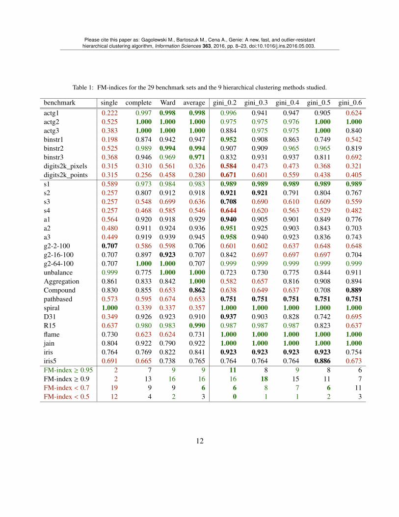
Let us compare the performance of the Genie algorithm (with F set to be the Gini-index; five different thresholds, g ∈ 0.2, 0.3, . . . , 0.6, are used) as well as the single, aver-age, complete, and Ward linkage schemes (as implemented in the hclust() function fromthe R [52] package stats). In order to do so, we compute the values of FM-index(C,C′),where C denotes the vector of true (reference) cluster labels (as described in Section 3.2),while C′ is the clustering obtained by cutting at an appropriate level the dendrogram re-turned by a hierarchical clustering algorithm being investigated. However, please observethat for some benchmark data sets the distance matrices consist of non-unique elements.As a result, the output of the algorithms may vary slightly from call to call (this is the caseof all the tested methods). Therefore, we shall report the median FM-index across 10 runsof randomly permuted observations in each benchmark set.

Table 1 gives the FM-indices for the 9 clustering methods and the 29 benchmark sets.Best results are marked with bold font. Aggregated basic summary statistics (minimum,quartiles, maximum, arithmetic mean, and standard deviation) for all the benchmark setsare provided in Table 2. Moreover, Figure 4 depicts violin plots of the FM-index distribu-tion1.

The highest mean and median FM scores were obtained for the Genie algorithm witha threshold of g = 0.2. This setting also leads to the best minimal (worst-case) FM-index.A general observation is that all the tested Gini-index thresholds gave the lowest variancein the FM-indices.

It is of course unsurprising that there is no free lunch in data clustering – no algo-rithm is perfect on all the data sets. All the tested hierarchical clustering algorithms werefar from perfect (FM < 0.7) on the digits2k_pixels, digits2k_points, and s4 data

1A violin depicts a box-and-whisker plot (boxes range from the 1st to the 3rd quartile, the median ismarked with a white dot) together with a kernel density estimator of the empirical distribution.

11


Table 1: FM-indices for the 29 benchmark sets and the 9 hierarchical clustering methods studied.

benchmark single complete Ward average gini_0.2 gini_0.3 gini_0.4 gini_0.5 gini_0.6actg1 0.222 0.997 0.998 0.998 0.996 0.941 0.947 0.905 0.624actg2 0.525 1.000 1.000 1.000 0.975 0.975 0.976 1.000 1.000actg3 0.383 1.000 1.000 1.000 0.884 0.975 0.975 1.000 0.840binstr1 0.198 0.874 0.942 0.947 0.952 0.908 0.863 0.749 0.542binstr2 0.525 0.989 0.994 0.994 0.907 0.909 0.965 0.965 0.819binstr3 0.368 0.946 0.969 0.971 0.832 0.931 0.937 0.811 0.692digits2k_pixels 0.315 0.310 0.561 0.326 0.584 0.473 0.473 0.368 0.321digits2k_points 0.315 0.256 0.458 0.280 0.671 0.601 0.559 0.438 0.405s1 0.589 0.973 0.984 0.983 0.989 0.989 0.989 0.989 0.989s2 0.257 0.807 0.912 0.918 0.921 0.921 0.791 0.804 0.767s3 0.257 0.548 0.699 0.636 0.708 0.690 0.610 0.609 0.559s4 0.257 0.468 0.585 0.546 0.644 0.620 0.563 0.529 0.482a1 0.564 0.920 0.918 0.929 0.940 0.905 0.901 0.849 0.776a2 0.480 0.911 0.924 0.936 0.951 0.925 0.903 0.843 0.703a3 0.449 0.919 0.939 0.945 0.958 0.940 0.923 0.836 0.743g2-2-100 0.707 0.586 0.598 0.706 0.601 0.602 0.637 0.648 0.648g2-16-100 0.707 0.897 0.923 0.707 0.842 0.697 0.697 0.697 0.704g2-64-100 0.707 1.000 1.000 0.707 0.999 0.999 0.999 0.999 0.999unbalance 0.999 0.775 1.000 1.000 0.723 0.730 0.775 0.844 0.911Aggregation 0.861 0.833 0.842 1.000 0.582 0.657 0.816 0.908 0.894Compound 0.830 0.855 0.653 0.862 0.638 0.649 0.637 0.708 0.889pathbased 0.573 0.595 0.674 0.653 0.751 0.751 0.751 0.751 0.751spiral 1.000 0.339 0.337 0.357 1.000 1.000 1.000 1.000 1.000D31 0.349 0.926 0.923 0.910 0.937 0.903 0.828 0.742 0.695R15 0.637 0.980 0.983 0.990 0.987 0.987 0.987 0.823 0.637flame 0.730 0.623 0.624 0.731 1.000 1.000 1.000 1.000 1.000jain 0.804 0.922 0.790 0.922 1.000 1.000 1.000 1.000 1.000iris 0.764 0.769 0.822 0.841 0.923 0.923 0.923 0.923 0.754iris5 0.691 0.665 0.738 0.765 0.764 0.764 0.764 0.886 0.673FM-index ≥ 0.95 2 7 9 9 11 8 9 8 6FM-index ≥ 0.9 2 13 16 16 16 18 15 11 7FM-index < 0.7 19 9 9 6 6 8 7 6 11FM-index < 0.5 12 4 2 3 0 1 1 2 3

12


Table 2: Basic summary statistics of the FM-index distribution over the 29 benchmark sets.

single complete Ward average gini_0.2 gini_0.3 gini_0.4 gini_0.5 gini_0.6Min 0.198 0.256 0.337 0.280 0.582 0.473 0.473 0.368 0.321Q1 0.349 0.623 0.674 0.707 0.723 0.697 0.751 0.742 0.648Median 0.564 0.874 0.918 0.918 0.921 0.909 0.901 0.843 0.751Q3 0.707 0.946 0.983 0.983 0.975 0.975 0.975 0.965 0.894Max 1.000 1.000 1.000 1.000 1.000 1.000 1.000 1.000 1.000Mean 0.554 0.782 0.820 0.812 0.850 0.840 0.834 0.815 0.752St.Dev. 0.235 0.225 0.188 0.215 0.147 0.156 0.159 0.172 0.185

0.2

0.4

0.6

0.8

1.0

single complete ward average gini_0.2 gini_0.3 gini_0.4 gini_0.5 gini_0.6

Figure 4: Violin plots of the FM-index distribution over the 29 benchmark sets.

13


Table 3: Basic summary statistics of the FM-index distribution over the 21 Euclidean benchmark sets.

single complete ward average gini_0.2 gini_0.3 gini_0.4 gini_0.5 gini_0.6 BIRCH k-meansMin 0.257 0.339 0.337 0.357 0.582 0.602 0.563 0.529 0.482 0.350 0.327Q1 0.480 0.623 0.674 0.707 0.723 0.697 0.751 0.742 0.695 0.653 0.701

Median 0.691 0.833 0.842 0.862 0.923 0.905 0.828 0.843 0.754 0.894 0.821Q3 0.764 0.920 0.924 0.936 0.987 0.987 0.987 0.923 0.911 0.924 0.969

Max 1.000 1.000 1.000 1.000 1.000 1.000 1.000 1.000 1.000 1.000 1.000Mean 0.629 0.777 0.803 0.812 0.850 0.841 0.833 0.828 0.789 0.801 0.816

St.Dev. 0.224 0.187 0.177 0.172 0.150 0.146 0.145 0.138 0.156 0.183 0.177

sets. However, in overall, the single linkage clustering is particularly bad (except for theunbalance and spiral data sets). Among the other algorithms, the complete linkage andthe Genie algorithm for g ≥ 0.5 give the lowest average and median FM-index. All theother methods (Genie with thresholds of g < 0.5, Ward, average linkage) are very com-petitive. Also please keep in mind that for the Genie algorithm with a low inequity indexthreshold we expect a loss in performance for unbalanced clusters sizes

Finally, let us compare the performance of the 9 hierarchical clustering algorithms aswell as the k-means and BIRCH (threshold=0.5, branching_factor=10) procedures(both implemented in the scikit-learn package for Python). Now we are of courselimited only to data in the Euclidean space, therefore the number of benchmark data setsreduces to 21. Table 3 gives basic summary statistics of the FM-index distributions. Wesee that in this case the Genie algorithm (g < 0.5) outperforms all the methods beingcompared too.

Taking into account our algorithm’s out-standing performance and – as it shall turnout in the next section – relatively low run-times (especially on larger data sets and com-pared with the average or Ward linkage), the proposed method may be recommended forpractical use.

4. Possible implementations of the Genie linkage algorithm

Having shown the high usability of the new approach, let us discuss some ways toimplement the Genie clustering method in very detail. We have already stated that themost important part of computing the single linkage algorithm consists of determining aminimal spanning tree (this can be non-unique if there are pairs of objects with identicaldissimilarity degrees) of the complete undirected weighted graph corresponding to objectsin X and the pairwise dissimilarities. It turns out that we have what follows.

Theorem 1. The Genie linkage criterion can be implemented based on an MST.

14


Sketch of the proof. By [51, Principle 2], in order to construct a minimal spanning tree,it is sufficient to connect any two disconnected minimal spanning subtrees via an edge ofminimal weight and iterate such a process until a single connected tree is obtained. As ourlinkage criterion (Section 3.1) always chooses such an edge, the proof is complete.

0. Input: x(1), . . . , x(n) – n objects, g ∈ (0, 1] – inequity index threshold,d – a dissimilarity measure;

1. ds = DisjointSets(1, 2, . . . , n);2. m = MST(x(1), . . . , x(n)); /* see Theorem 1 */

3. pq = MinPriorityQueue<PQItem>(∅);/* PQItem structure: (index1, index2, dist);

pq returns the element with the smallest dist */

4. for each weighted edge (i, j, di, j) in m:4.1. pq.push(PQItem(i, j,di, j));

5. for j = 1, 2, . . . , n − 1:5.1. if ds.compute_inequity() ≤ g: /* e.g., the Gini-index */

5.1.1. t = pq.pop(); /* PQItem with the least dist */

else:5.1.2. t = pq.pop_conditional

(t: ds.size(t.index1) = ds.min_size()

or ds.size(t.index2) = ds.min_size());

/* PQItem with the least dist that fulfills the given logical condition */

5.2. s1 = ds.find_set(t.index1);5.3. s2 = ds.find_set(t.index2); /* assert: s1 , s2 */

5.4. output “linking (s1, s2)”;5.5. ds.link(t.index1, t.index2);

Figure 5: A pseudocode for the Genie algorithm.

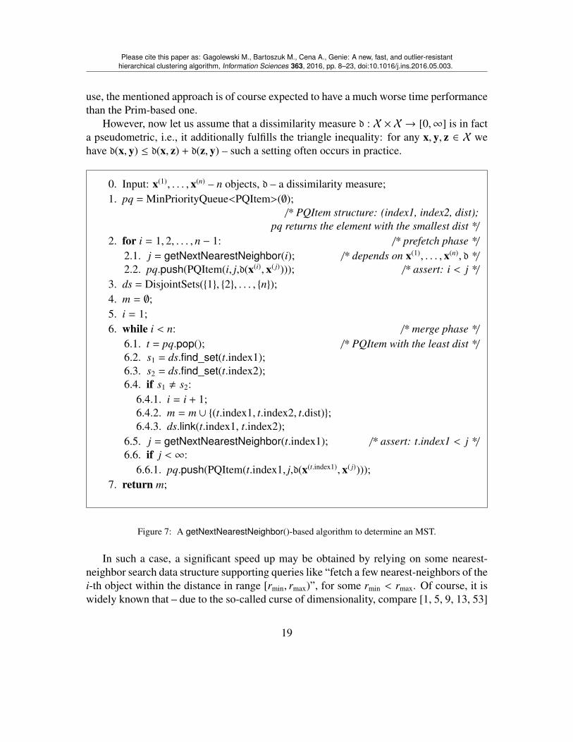
Please note that, by definition, the weighted edges appear in an MST in no particularorder – for instance, the Prim [51] algorithm’s output depends on the permutation of inputs.Therefore, having established the above relation between the Genie clustering and an MST,in Figure 5 we provide a pseudocode of the algorithm that guarantees the right clustermerge order. The procedure resembles the Kruskal [37] algorithm and is fully concordantwith our method’s description in Section 3.1.

15


Observe that the very same algorithm can be used to compute the single linkage clus-tering (in such a case, step 5.1 – in which we compute a chosen inequity measure – aswell as step 5.1.2 – in which we test whether the inequity measure raises above a giventhreshold – are never executed).

Example 1. Let us consider an exemplary data set consisting of 5 points in the real line:x(1) = 0, x(2) = 1, x(3) = 3, x(4) = 6, x(5) = 10 and let us set d to be the Euclidean dis-tance. The minimum spanning tree – which, according to Theorem 1 gives us completeinformation needed to compute the resulting clustering – consists of the following edges:x(1), x(2), x(2), x(3), x(3), x(4), x(4), x(5), with weights 1, 2, 3, and 4, respectively.

Let the inequity measure F be the Gini-index. If the threshold g is set to 1.0 (the singlelinkage), the merge steps are as follows. Please note that the order in which we merge theclusters is simply determined by sorting the edges in the MST increasingly by weights, justas in the Kruskal algorithm.

step current partitioning MST edge Gini-index0. x(1), x(2), x(3), x(4), x(5) x(1), x(2)1 0.01. x(1), x(2), x(3), x(4), x(5) x(2), x(3)2 0.22. x(1), x(2), x(3), x(4), x(5) x(3), x(4)3 0.43. x(1), x(2), x(3), x(4), x(5) x(4), x(5)4 0.64. x(1), x(2), x(3), x(4), x(5) — —

However, if the threshold is set to g = 0.3, then when proceeding form step 2 to step3, we need to link x(4) and x(5) instead of x(1), x(2), x(3) and x(4) – that is, the mergeis based now on a different MST edge: x(4), x(5)4 instead of x(3), x(4)3. Therefore, the re-sulting 2-partition will be different than the above one: we obtain x(1), x(2), x(3), x(4), x(5)

(Gini-index = 0.2).

4.1. Implementation detailsIn this study, we decided to focus on the Gini-index. In order to make the algorithm

time-efficient, this inequity index must be computed incrementally. Let g j denote the Gini-index value at the time when there are n − j clusters, j = 0, 1, . . . , n − 1. Initially, wheneach cluster is of size 1, the Gini-index is of course equal to 0, hence g0 = 0. Assume thatwhen proceeding from step j − 1 to j we link clusters of sizes cs1 and cs2 . It can easily beshown that:

g j =(n − j) n g j−1 +

∑n− j+1i=1

(|ci − cs1 − cs2 | − |ci − cs1 | − |ci − cs2 |

)− cs2 − cs1 + |cs1 − cs2 |

(n − j − 1) n.

16


In other words, after each merge operation, the index is updated, which requires O(n) op-erations instead of O(n2) when the index is recomputed from scratch based on the originalformula (1). On a side note, it might be shown that the Gini-index can be written as alinear combination of order statistics (compare, e.g., the notion of an OWA operator), butthe use of such a definition would require sorting the cluster size vector in each iterationor relying on an ordered search tree-like data structure.

Moreover, please note that the algorithm is based on a non-standard implementation ofthe disjoint sets data structure. Basically, the required extension that keeps track of clustercounts can be implemented quite easily.

The implementation of the pop_conditional() method in the priority queue pq (weused a heap-based data structure) can be done by means of an auxiliary queue, onto whichelements not fulfilling the logical condition given in step 5.1.2 are temporarily moved.If, after a merge operation, the inequity index is still above the desired threshold andthe minimal cluster size did not change since the previous iteration, the auxiliary priorityqueue is kept as-is and we continue to seek a cluster of the lowest cardinality from thesame place. Otherwise, the elements must go back to pq and the search must start over.

To conclude, the cost of applying the cluster merge procedure (O(n2) pessimisticallyfor g < 1 and O(n log n) for g = 1) is not dominated by the cost of determining an MST(O(Cn2) pessimistically, under our assumptions this involves a function C of data dimen-sionality and reflects the cost of computing a given dissimilarity measure d). Hence, thenew clustering scheme shall give us run-times that are comparable with the single link-age method. It is worth noting that the time complexity (Θ(n2)) as well as the memorycomplexity (Θ(n)) of the algorithm is optimal (as far as the whole class of hierarchicalclustering algorithms is concerned, compare [41]).

On a side note, the NN-chains algorithm, which is suitable for solving – among others– the complete, average, and Ward linkage clustering also has a time complexity of O(n2)[41, 43], but, as we shall see in further on, it requires computing at least 2–5 times morepairwise distances.

For the sake of comparison, let us study two different algorithms to determine an MST.

1. An MST algorithm based on Prim’s one. A first algorithm, sketched in [45, Figure 8],is quite similar to the one by Prim [51]. Its pseudocode is given in Figure 6. Note that thealgorithm guarantees that exactly (n2 − n)/2 pairwise distances are computed. Moreover,the inner loop can be run in parallel. In such a case, M should be a vector of indices notyet in the MST – due to that the threads may have random access to such an array – andstep 6.2.3 should be moved to a separate loop – so as to a costly critical section is avoided.

17


0. Input: x(1), . . . , x(n) – n objects, d – a dissimilarity measure;1. F = (∞, . . . ,∞) (n times); /* F j – index of j’s nearest neighbor */

2. D = (∞, . . . ,∞) (n times); /* D j – distance to j’s nearest neighbor */

3. lastj = 1;4. m = ∅; /* a resulting MST */

5. M = 2, 3, . . . , n; /* indices not yet in m */

6. for i = 1, 2, . . . , n − 1:6.1. bestj = 1;6.2. for each j ∈ M:

6.2.1. d = d(x(lastj), x( j));6.2.2. if d < D j:

6.2.2.1. D j = d;6.2.2.2. F j = lastj;

6.2.3. if D j < Dbestj: /* assert: D1 = ∞ */

6.2.3.1. bestj = j;6.3. m = m ∪ (Fbestj, bestj,Dbestj); /* add an edge to m */

6.4. M = M \ bestj; /* now this index is in m */

6.5. lastj = bestj;7. return m;

Figure 6: A simple (n2 − n)/2 algorithm to determine an MST.

2. An MST algorithm based on Kruskal’s one. The second algorithm considered is basedon the one by Kruskal [37] and its pseudocode is given in Figure 7. It relies on a methodcalled getNextNearestNeighbor(), which fetches the index j of the next not-yet consid-ered nearest (in terms of increasing d) neighbor of an object at index i having the propertythat j > i. If such a neighbor does not exist anymore, the function returns ∞. Pleaseobserve that in the prefetch phase the calls to getNextNearestNeighbor() can be run inparallel.

A naïve implementation of the getNextNearestNeighbor() function requires eitherO(1) time and O(n) memory for each object (i.e., O(n2) in total – the lists of all neighborscan be stored in n priority queues, one per each object) or O(n) time and O(1) memory(i.e., O(n) in total – no caching done at all). As our priority is to retain total O(n) memory

18


use, the mentioned approach is of course expected to have a much worse time performancethan the Prim-based one.

However, now let us assume that a dissimilarity measure d : X × X → [0,∞] is in facta pseudometric, i.e., it additionally fulfills the triangle inequality: for any x, y, z ∈ X wehave d(x, y) ≤ d(x, z) + d(z, y) – such a setting often occurs in practice.

0. Input: x(1), . . . , x(n) – n objects, d – a dissimilarity measure;1. pq = MinPriorityQueue<PQItem>(∅);

/* PQItem structure: (index1, index2, dist);pq returns the element with the smallest dist */

2. for i = 1, 2, . . . , n − 1: /* prefetch phase */

2.1. j = getNextNearestNeighbor(i); /* depends on x(1), . . . , x(n), d */

2.2. pq.push(PQItem(i, j,d(x(i), x( j)))); /* assert: i < j */

3. ds = DisjointSets(1, 2, . . . , n);4. m = ∅;5. i = 1;6. while i < n: /* merge phase */

6.1. t = pq.pop(); /* PQItem with the least dist */

6.2. s1 = ds.find_set(t.index1);6.3. s2 = ds.find_set(t.index2);6.4. if s1 , s2:

6.4.1. i = i + 1;6.4.2. m = m ∪ (t.index1, t.index2, t.dist);6.4.3. ds.link(t.index1, t.index2);

6.5. j = getNextNearestNeighbor(t.index1); /* assert: t.index1 < j */

6.6. if j < ∞:6.6.1. pq.push(PQItem(t.index1, j,d(x(t.index1), x( j))));

7. return m;

Figure 7: A getNextNearestNeighbor()-based algorithm to determine an MST.

In such a case, a significant speed up may be obtained by relying on some nearest-neighbor search data structure supporting queries like “fetch a few nearest-neighbors of thei-th object within the distance in range [rmin, rmax)”, for some rmin < rmax. Of course, it iswidely known that – due to the so-called curse of dimensionality, compare [1, 5, 9, 13, 53]

19


– there is no general-purpose algorithm which always works better than the naïve methodin spaces of high dimension. Nevertheless, in our case, some modifications of a chosendata structure may lead to improvements in time performance.

Our carefully tuned-up reference implementation (discussed below) is based on a van-tage point (VP)-tree, see [57]. The most important modifications applied are as follows.

• Each tree node stores an information on the maximal object index that can be foundin its subtrees. This speeds up the search for NNs of objects with higher indices. Nodistance computation are performed for a pair of indices (i, j) unless i < j.

• Each tree node includes an information whether all its subtrees store elements fromthe same set in the disjoint sets data structure ds. This Boolean flag is recursively up-dated during a call to getNextNearestNeighbor(). Due to that, a significant numberof tree nodes during the merge phase can be pruned.

• An actual tree query returns a batch of nearest-neighbors of adaptive size between20 and 256 (the actual count is determined automatically according to how the un-derlying VP-tree prunes the child nodes during the search). The returned set ofnearest-neighbors is cached in a separate priority queue, one per each input datapoint. Note that the size of the returned batch guarantees asymptotic linear totalmemory use.

4.2. The genie package for RA reference implementation of the Genie algorithm has been included in the genie

package for R [52]. This software is distributed under the open source GNU GeneralPublic License, version 3. The package is available for download at the official CRAN(Comprehensive R Archive Network) repository, see https://cran.r-project.org/web/packages/genie/, and hence can be installed from within an R session via a callto install.packages("genie"). All the core algorithms have been developed in theC++11 programming language; the R interface has been provided by means of the Rcpp[17] package. What is more, we decided to rely on the OpenMP API in order to enablemulti-threaded computations.

A data set’s clustering can be determined via a call to the genie::hclust2() func-tion. The objects argument, with which we provide a data set to be clustered, maybe a numeric matrix, a list of integer vectors, or an R character vector. The dissimi-larity measure is selected via the metric argument, e.g., "euclidean", "manhattan","maximum", "hamming", "levenshtein", "dinu", etc. The thresholdGini argumentcan be used to define the threshold for the Gini-index (denoted with g in Figure 5). Fi-nally, the useVpTree argument can be used to switch between the MST algorithms given

20

https://cran.r-project.org/web/packages/genie/

https://cran.r-project.org/web/packages/genie/


in Figures 6 (the default) and 7. For more details, please refer to the function’s manualpage (?genie::hclust2).

Here is an exemplary R session in which we compute the clustering of the flame dataset.

# load the ‘flame‘ benchmark data set,# see http://www.gagolewski.com/resources/data/clustering/data <- as.matrix(read.table(gzfile("flame.data.gz")))labels <- scan(gzfile("flame.labels.gz"), quiet=TRUE)

# run the Genie algorithm, threshold g=0.2result <- genie::hclust2(objects=data, metric="euclidean",

thresholdGini=0.2)

# get the number of reference clustersk <- length(unique(labels))

# plot the resultsplot(data[,1], data[,2], col=labels, pch=cutree(result, k))

# compute the FM-indexas.numeric(dendextend::FM_index(labels, cutree(result, k),

include_EV=FALSE))## [1] 1

4.3. Number of calls to the dissimilarity measureLet us compare the number of calls to the dissimilarity measure d required by different

clustering algorithms. The measures shall be provided relative to (n2 − n)/2, which isdenoted with “100%”.

The benchmark data sets are generated as follows. For a given n, σ, and d, k = 10cluster centers µ(1), . . . ,µ(k) are picked randomly from the uniform distribution on [0, 10]d.Then, each of the n observations is generated as µ( j) + y, where yl for each l = 1, . . . , d is arandom variate from the normal distribution with expectation of 0 and standard deviationof σ and j is a random number distributed uniformly in 1, 2, . . . , k. In other words, sucha data generation method is more or less equivalent to the one used in case of the g2 datasets in the previous section. Here, d is set to be the Euclidean metric.

21


Table 4: Relative number of pairwise distance computations (as compared to (n2 − n)/2) together withFM-indices (in parentheses).

σ d n gini_0.3 gini_1.0 complete Ward average(single)

0.50 2 10000 ∗4.8% (0.76) 100% (0.38) 476% (0.72) 204% (0.80) 484% (0.78)0.50 5 10000 ∗22.0% (1.00) 100% (0.86) 493% (1.00) 221% (1.00) 496% (1.00)1.50 10 10000 ∗30.3% (0.96) 100% (0.32) 496% (0.98) 240% (0.98) 499% (0.91)1.50 15 10000 ∗58.3% (1.00) 100% (0.42) 497% (1.00) 253% (1.00) 498% (0.98)1.50 20 10000 ∗84.9% (1.00) 100% (0.69) 497% (1.00) 261% (1.00) 498% (1.00)3.50 100 10000 ∗101.8% (1.00) 100% (0.32) 498% (1.00) 299% (1.00) 499% (1.00)5.00 250 10000 ∗100.9% (0.99) 100% (0.32) 498% (1.00) 312% (1.00) 499% (1.00)1.5 10 100000 ∗14.1% (0.94) 100% (0.32) — 241% (0.98) —3.5 100 100000 ∗104.0% (0.98) 100% (0.32) — † 321% (0.99) —

(∗) – a VP-tree used (Fig. 7) to determine an MST; the (n2 − n)/2 algorithm (Fig. 6) could always be usedinstead.(†) – only one run of the experiment was conducted.

In each test case (different choices of n, d, σ), we randomly generated ten differentdata sets and averaged the resulting FM-indices and relative numbers of calls to d. Table 4compares:

• the Genie algorithm (genie::hclust2(), package version 1.0.0) based on each ofthe aforementioned MST algorithms (useVpTree equals either to TRUE or FALSE);the Gini-index threshold of 0.3 and 1.0, the latter is equivalent to the single linkagecriterion,

• the Ward linkage (the hclust.vector() function from the fastcluster 1.1.16package [42] – this implementation works only in the case of the Euclidean distancebut uses O(n) memory),

• the complete and average linkage (fastcluster::hclust() – they use an NN-chains-based algorithm, and require a pre-computed distance matrix, therefore uti-lizing O(n2) memory).

We observe a positive impact of using a metric tree data structure (useVpTree=TRUE)in low-dimensional spaces. In high-dimensional spaces, it is better to rely on the (n2 −

n)/2 (Prim-like) algorithm. Nevertheless, we observe that in high dimensional spaces therelative number of calls to the dissimilarity measure is 2–5 times smaller than in the case ofother linkages. Please note that an NN-chains-based version of the Ward linkage (not listed

22


in the table; fastcluster::hclust()) gives similar results as the complete and averageones and that its Euclidean-distance specific version (fastcluster::hclust.vector())seems to depend on the data set dimensionality.

4.4. Exemplary run-timesLet us inspect exemplary run-time measurements of the genie::hclust2() function

(genie package version 1.0.0). The measurements were performed on a laptop with aQuad-core Intel(R) Core(TM) i7-4700HQ @ 2.40GHz CPU and 16 GB RAM. The com-puter was running Fedora 21 Linux (kernel 4.1.13-100) and the gcc 4.9.2 compiler wasused (-O2 -march=native optimization flags).

Table 5: Exemplary run-times (in seconds) for different thread numbers, n = 100,000.

Number of threadsdata MST algorithm g 1 2 4d = 10, σ = 1.5 Fig. 7 with a VP-tree 0.3 46.5 33.4 28.2

Fig. 6 0.3 91.5 59.9 44.8Fig. 7 with a VP-tree 1.0 32.0 19.1 13.4Fig. 6 1.0 77.5 47.7 31.6

d = 100, σ = 3.5 Fig. 7 with a VP-tree 0.3 1396 740 456Fig. 6 0.3 743 413 293Fig. 7 with a VP-tree 1.0 1385 717 454Fig. 6 1.0 734 396 281

Table 5 summarizes the results for n = 100,000 and 1, 2, as well as 4 threads (setup via the OMP_THREAD_LIMIT environmental variable). The experimental data sets weregenerated in the same manner as above. The reported times are minimums of 3 runs. Notethat the results also include the time needed to generate some additional objects, so thatthe output is of the same form as the one generated by the stats::hclust() functionin R.

We note that running 4 threads at a time (on a single multi-core CPU) gives us a2–3-fold speed-up. Moreover, a VP-tree-based implementation (Figure 7, useVpTree=TRUE)is twice as costly as the other one in spaces of high dimensions. However, in spaces oflow dimension it outperforms the (n2 − n)/2 approach (Figure 6). Nevertheless, if a user isunsure whether he/she deals with a high- or low-dimensional space and n is of moderateorder of magnitude, the simple approach should rather be recommended, as it gives muchmore predictable timings. This is why we have decided that the useVpTree argumentshould default to FALSE.

23


For a point of reference, let us note that a single test run of the Ward algorithm(fastcluster::hclust.vector(), single-threaded) for n = 100,000, d = 10, σ = 1.5required 1452.8 seconds and for d = 100, σ = 3.5 – as much as 18433.7 seconds (whichis almost 25 times slower than the Genie approach).

5. Conclusions

We have presented a new hierarchical clustering linkage criterion which is based onthe notion of an inequity (poverty) index. The performed benchmarks indicate that theproposed algorithm – unless the underlying cluster structure is drastically unbalanced –works in overall better not only than the widely used average and Ward linkage scheme,but also than the k-means and BIRCH algorithms which can be applied on data in theEuclidean space only.

Our method requires up to (n2 − n)/2 distance computations, which is ca. 2–5 timesless than in the case of the other popular linkage schemes. Its performance is comparablewith the single-linkage clustering. As there is no need to store the full distance matrix, thealgorithm can be used to cluster larger (within one order of magnitude) data sets than withthe Ward and average linkage schemes.

Nevertheless, it seems that we have reached a kind of general limit of an input dataset size for “classical” hierarchical clustering, especially in case of multidimensional data.Due to the curse of dimensionality, we do not have any nearest-neighbor search data struc-tures that would enable us to cluster data sets of sizes greater than few millions of obser-vations in a reasonable time span. What is more, we should keep in mind that the lowerbound for run-times of all the hierarchical clustering methods is Ω(n2) anyway. However,let us stress that for smaller (non-big-data) samples, hierarchical clustering algorithms arestill very useful. This is due to the fact that they do not require a user to provide the desirednumber of clusters in advance and that only a measure of objects’ dissimilarity – fulfillingvery mild properties – must be provided in order to determine a data partition.

Further research on the algorithm shall take into account the effects of, e.g., choos-ing different inequity measures or relying on approximate nearest-neighbors search algo-rithms and data dimension reduction techniques on the clustering quality. Moreover, in adistributed environment, one may consider partitioning subsets of input data individuallyand then rely on some clustering aggregation techniques, compare, e.g., [26].

Finally, let us note that the Genie algorithm depends on a free parameter, namely,the inequity index merge threshold, g. The existence of such a tuning parameter is anadvantage, as a user may select its value to suit her/his needs. In the case of the Gini-index,we recommend the use of g ∈ [0.2, 0.5), depending on our knowledge of the underlyingcluster distribution. Such a choice led to outstanding results during benchmark studies.

24


However, we should keep in mind that if the threshold is too low, the algorithm mighthave problems with correctly identifying clusters of smaller sizes in case of unbalanceddata. On the other hand, g cannot be too large, as the algorithm might start to behaveas the single-linkage method, which has a very poor performance. A possible way toautomate the choice of g could consist of a few pre-flight runs (for different thresholds)on a randomly chosen data sample, a verification of the obtained preliminary clusterings’qualities, and a choice of the best coefficient for the final computation.

Acknowledgments

We would like to thank the Anonymous Reviewers for the constructive comments thathelped to significantly improve the manuscript’s quality. Moreover, we are indebted toŁukasz Błaszczyk for providing us with the scikit-learn algorithms performance re-sults.

This study was supported by the National Science Center, Poland, research project2014/13/D/HS4/01700. Anna Cena and Maciej Bartoszuk would like to acknowledge thesupport by the European Union from resources of the European Social Fund, Project POKL “Information technologies: Research and their interdisciplinary applications”, agree-ment UDA-POKL.04.01.01-00-051/10-00 via the Interdisciplinary PhD Studies Program.

References

[1] C.C. Aggarwal, A. Hinneburg, D.A. Keimn, On the surprising behavior of distancemetric in high-dimensional space, Lecture Notes in Computer Science 1973 (2001)420–434.

[2] O. Aristondo, J. García-Lapresta, C. Lasso de la Vega, R. Marques Pereira, Classicalinequality indices, welfare and illfare functions, and the dual decomposition, FuzzySets and Systems 228 (2013) 114–136.

[3] G. Beliakov, S. James, Unifying approaches to consensus across different preferencerepresentations, Applied Soft Computing 35 (2015) 888–897.

[4] G. Beliakov, S. James, D. Nimmo, Can indices of ecological evenness be used tomeasure consensus?, in: Proc. IEEE Intl. Conf. Fuzzy Systems’15, Beijing, China,2014, pp. 1–8.

[5] K. Beyer, J. Goldstein, R. Ramakrishnan, U. Shaft, When is nearest neighbor mean-ingful?, in: C. Beeri, P. Buneman (Eds.), Proc. ICDT, Springer-Verlag, 1998, pp.217–235.

25


[6] J.C. Bezdek, Pattern Recognition with Fuzzy Objective Function Algorithms,Springer, 1981.

[7] C. Bonferroni, Elementi di statistica generale, Libreria Seber, Firenze, 1930.

[8] S. Bortot, R. Marques Pereira, On a new poverty measure constructed from the ex-ponential mean, in: Proc. IFSA/EUSFLAT’15, Gijon, Spain, 2015, pp. 333–340.

[9] S. Brin, Near neighbor search in large metric spaces, in: In Proceedings of the 21thInternational Conference on Very Large Data Bases, Morgan Kaufmann Publishers,1995, pp. 574–584.

[10] R. Cai, Z. Zhang, A.K. Tung, C. Dai, Z. Hao, A general framework of hierarchicalclustering and its applications, Information Sciences 272 (2014) 29–48.

[11] J. Camargo, Must dominance increase with the number of subordinate species incompetitive interactions?, Journal of Theoretical Biology 161 (1993) 537–542.

[12] H. Chang, D. Yeung, Robust path-based spectral clustering, Pattern Recognition 41(2008) 191–203.

[13] E. Chavez, G. Navarro, R. Baeza-Yates, J.L. Marroquin, Searching in metric spaces,ACM Computing Surveys 33 (2001) 273–321.

[14] S. Dasgupta, Performance guarantees for hierarchical clustering, in: Proceedings ofthe Conference on Learning Theory, 2002, pp. 351–363.

[15] I. Dimitrovski, D. Kocev, S. Loskovska, S. Džeroski, Improving bag-of-visual-wordsimage retrieval with predictive clustering trees, Information Sciences 329 (2016)851–865.

[16] L.P. Dinu, R.T. Ionescu, Clustering methods based on closest string via rank distance,in: 14th Intl. Symp. Symbolic and Numeric Algorithms for Scientific Computing,IEEE, 2012, pp. 207–213.

[17] D. Eddelbuettel, Seamless R and C++ Integration with Rcpp, Springer, New York,2013.

[18] L.N. Ferreira, L. Zhao, Time series clustering via community detection in networks,Information Sciences 326 (2016) 227–242.

[19] R. Fisher, The use of multiple measurements in taxonomic problems, Annals of Eu-genics 7 (1936) 179–188.

26


[20] E. Fowlkes, C. Mallows, A method for comparing two hierarchical clusterings, Jour-nal of the American Statistical Association 78 (1983) 553–569.

[21] P. Fränti, O. Virmajoki, Iterative shrinking method for clustering problems, PatternRecognition 39 (2006) 761–765.

[22] L. Fu, E. Medico, FLAME, a novel fuzzy clustering method for the analysis of DNAmicroarray data, BMC bioinformatics 8 (2007) 3.

[23] M. Gagolewski, Spread measures and their relation to aggregation functions, Euro-pean Journal of Operational Research 241 (2015) 469–477.

[24] J. García-Lapresta, C. Lasso de la Vega, R. Marques Pereira, A. Urrutia, A new classof fuzzy poverty measures, in: Proc. of IFSA/EUSFLAT2015, Gijon, Spain, 2015,pp. 1140–1146.

[25] C. Gini, Variabilità e mutabilità, C. Cuppini, Bologna, 1912.

[26] A. Gionis, H. Mannila, P. Tsaparas, Clustering aggregation, ACM Transactions onKnowledge Discovery from Data 1 (2007) 4.

[27] J. Gower, G. Ross, Minimum spanning trees and single linkage cluster analysis, Jour-nal of the Royal Statistical Society. Series C (Applied Statistics) 18 (1969) 54–64.

[28] R. Graham, P. Hell, On the history of the minimum spanning tree problem, Annalsof the History of Computing 7 (1985) 43–57.

[29] D. Gómez, E. Zarrazola, J. Yáñez, J. Montero, A divide-and-link algorithm for hier-archical clustering in networks, Information Sciences 316 (2015) 308–328.

[30] Z. Halim, M. Waqas, S.F. Hussain, Clustering large probabilistic graphs using multi-population evolutionary algorithm, Information Sciences 317 (2015) 78–95.

[31] T. Hastie, R. Tibshirani, J. Friedman, The Elements of Statistical Learning: DataMining, Inference, and Prediction, Springer, 2013.

[32] C. Heip, A new index measuring evenness, Journal of Marine Biological Associationof the United Kingdom 54 (1974) 555–557.

[33] A. Jain, M. Law, Data clustering: A user’s dilemma, Lecture Notes in ComputerScience 3776 (2005) 1–10.

27


[34] F. Jiang, G. Liu, J. Du, Y. Sui, Initialization of k-modes clustering using outlierdetection techniques, Information Sciences 332 (2016) 167–183.

[35] M. Kobus, Attribute decomposition of multidimensional inequality indices, Eco-nomics Letters 117 (2012) 189–191.

[36] M. Kobus, P. Miłos, Inequality decomposition by population subgroups for ordinaldata, Journal of Health Economics 31 (2012) 15–21.

[37] J.B. Kruskal, On the shortest spanning subtree of a graph and the traveling salesmanproblem, Proceedings of the American Mathematical Society 7 (1956) 48–50.

[38] I. Kärkkäinen, P. Fränti, Dynamic local search algorithm for the clustering problem,in: Proc. 16th Intl. Conf. Pattern Recognition’02, volume 2, IEEE, 2002, pp. 240–243.

[39] P. Legendre, L. Legendre, Numerical Ecology, Elsevier Science BV, Amsterdam,2003.

[40] J.B. MacQueen, Some methods for classification and analysis of multivariate ob-servations, in: Proc. Fifth Berkeley Symp. on Math. Statist. and Prob., volume 1,University of California Press, Berkeley, 1967, pp. 281–297.

[41] D. Müllner, Modern hierarchical, agglomerative clustering algorithms,ArXiv:1109.2378 [stat.ML] (2011).

[42] D. Müllner, fastcluster: Fast hierarchical, agglomerative clustering routines for R andPython, Journal of Statistical Software 53 (2013) 1–18.

[43] F. Murtagh, A survey of recent advances in hierarchical clustering algorithms, TheComputer Journal 26 (1983) 354–359.

[44] F. Murtagh, P. Legendre, Ward’s hierarchical agglomerative clustering method:Which algorithms implement ward’s criterion?, Journal of Classification 31 (2014)274–295.

[45] C.F. Olson, Parallel algorithms for hierarchical clustering, Parallel Computing 21(1995) 1313–1325.

[46] W. Pedrycz, Conditional fuzzy c-means, Pattern Recognition Letters 17 (1996) 625–631.

28


[47] W. Pedrycz, A. Bargiela, Granular clustering: A granular signature of data, IEEETransactions on Systems, Man, and Cybernetics, Part B: Cybernetics 32 (2002) 212–224.

[48] W. Pedrycz, J. Waletzky, Fuzzy clustering with partial supervision, IEEE Transac-tions on Systems, Man, and Cybernetics, Part B: Cybernetics 27 (1997) 787–795.

[49] E. Pielou, An Introduction to Mathematical Ecology, Wiley-Interscience, New York,1969.

[50] E. Pielou, Ecological Diversity, Wiley, New York, 1975.

[51] R. Prim, Shortest connection networks and some generalizations, Bell System Tech-nical Journal 36 (1957) 1389–1401.

[52] R Development Core Team, R: A language and environment for statistical comput-ing, R Foundation for Statistical Computing, Vienna, Austria, 2015. http://www.R-project.org.

[53] M. Radavanovic, A. Nanopoulos, M. Ivanovic, Hubs in space: Popular nearest neigh-bors in high-dimensional data, Journal of Machine Learning Research 11 (2010)2487–2531.

[54] F. Rohlf, Hierarchical clustering using the minimum spanning tree, The ComputerJournal 16 (1973) 93–95.

[55] C. Veenman, M. Reinders, E. Backer, A maximum variance cluster algorithm, IEEETransactions on Pattern Analysis and Machine Intelligence 24 (2002) 1273–1280.

[56] R. Xu, D.C. Wunsch II, Clustering, Wiley-IEEE Press, 2009.

[57] P.N. Yianilos, Data structures and algorithms for nearest neighbor search in generalmetric spaces, in: Proceedings of the Fourth Annual ACM-SIAM Symposium onDiscrete Algorithms, SODA ’93, Society for Industrial and Applied Mathematics,1993, pp. 311–321.

[58] C. Zahn, Graph-theoretical methods for detecting and describing gestalt clusters,IEEE Transactions on Computers C-20 (1971) 68–86.

[59] S. Zahra, M.A. Ghazanfar, A. Khalid, M.A. Azam, U. Naeem, A. Prugel-Bennett,Novel centroid selection approaches for kmeans-clustering based recommender sys-tems, Information Sciences 320 (2015) 156–189.

29


[60] T. Zhang, R. Ramakrishnan, M. Livny, BIRCH: An efficient data clustering methodfor very large databases, in: Proc. ACM SIGMOD’96 Intl. Conf. Management ofData, ACM, 1996, pp. 103–114.

30

genie: a new, fast, and outlier-resistant hierarchical ... · genie: a new, fast, and...

Documents