precast concrete elements for accelerated bridge...

Precast Concrete Elements for Accelerated Bridge Construction

Final ReportJanuary 2009

Sponsored bythe Iowa Highway Research Board (IHRB Project TR-561)andthe Iowa Department of Transportation (CTRE Project 06-262)

Iowa State University’s Center for Transportation Research and Education is the umbrella organization for the following centers and programs: Bridge Engineering Center • Center for Weather Impacts on Mobility

and Safety • Construction Management & Technology • Iowa Local Technical Assistance Program • Iowa Traffi c Safety Data Service • Midwest Transportation Consortium • National Concrete Pavement

Technology Center • Partnership for Geotechnical Advancement • Roadway Infrastructure Management and Operations Systems • Statewide Urban Design and Specifications • Traffic Safety and Operations

Volume 3. Laboratory Testing, Field Testing, and Evaluation of a Precast Concrete Bridge: Black Hawk County

About the Bridge Engineering Center

The mission of the Bridge Engineering Center is to conduct research on bridge technologies to help bridge designers/owners design, build, and maintain long-lasting bridges.

Disclaimer Notice

The contents of this report refl ect the views of the authors, who are responsible for the facts and the accuracy of the information presented herein. The opinions, fi ndings and conclusions expressed in this publication are those of the authors and not necessarily those of the sponsors.

The sponsors assume no liability for the contents or use of the information contained in this document. This report does not constitute a standard, specifi cation, or regulation.

The sponsors do not endorse products or manufacturers. Trademarks or manufacturers’ names appear in this report only because they are considered essential to the objective of the document.

Nondiscrimination Statement

Iowa State University does not discriminate on the basis of race, color, age, religion, national origin, sexual orientation, gender identity, sex, marital status, disability, or status as a U.S. veteran. Inquiries can be directed to the Director of Equal Opportunity and Diversity, (515) 294-7612.

GENERAL ABSTRACT

Precast Concrete Elements for Accelerated Bridge Construction

Precast concrete elements and accelerated bridge construction techniques have the potential to improve the health of the U.S. highway system. In precast bridge construction, the individual components are manufactured off-site and assembled on-site. This method usually increases the components’ durability, reduces on-site work and construction time, minimizes traffic disruption, and lowers life-cycle costs. Before widespread implementation, however, the benefits of precast elements and accelerated bridge construction must be verified in the laboratory and field.

For this project, precast bridge elements and accelerated bridge construction techniques were investigated in the laboratory and at three bridge projects in Iowa: in Boone County, Madison County, and Black Hawk County. The objectives were to evaluate the precast bridge elements, monitor the long-term performance of the completed bridges, and evaluate accelerated bridge construction techniques.

The results of these investigations are presented in three volumes, as described below; this volume is Volume 3.

Vol. 1-1. Laboratory Testing of Precast Substructure Components: Boone County Bridge 1-2. Laboratory Testing of Full-Depth Precast, Prestressed Concrete Deck Panels:

Boone County Bridge 1-3. Field Testing of a Precast Concrete Bridge: Boone County Bridge In 2006, a continuous four-girder, three-span bridge was constructed that included precast abutments, pier cap elements, prestressed beams, and precast full-depth deck panels. All of the precast elements performed well during strength testing and were set quickly and smoothly during construction, and the completed bridge experienced very small displacements and strains when subjected to live loads.

Vol. 2. Laboratory Testing, Field Testing, and Evaluation of a Precast Concrete Bridge: Madison County Bridge In 2007, a two-lane single-span bridge was constructed that had precast box girders with precast abutments. The elements performed well during laboratory load transfer and strength testing, and the completed bridge performed well in terms of maximum deflections and differential displacements between longitudinal girder joints.

Vol. 3. Laboratory Testing, Field Testing, and Evaluation of a Precast Concrete Bridge: Black Hawk County In 2007, two precast modified beam-in-slab bridge (PMBISB) systems were constructed, each of which included precast abutment caps, backwalls, and deck panels. Various deck panel configurations transferred load effectively during laboratory testing, and all precast elements met expectations. The completed bridges experienced very low induced stresses and met AASHTO deflection criteria, while the PMBSIB system effectively transferred load transversely.

Technical Report Documentation Page

1. Report No. 2. Government Accession No. 3. Recipient’s Catalog No. IHRB Project TR-561

4. Title and Subtitle 5. Report Date Precast Concrete Elements for Accelerated Bridge Construction: Laboratory Testing, Field Testing, and Evaluation of a Precast Concrete Bridge, Black Hawk County

January 2009 6. Performing Organization Code

7. Author(s) 8. Performing Organization Report No. Wayne Klaiber, Terry Wipf, Vernon Wineland CTRE Project 06-262 9. Performing Organization Name and Address 10. Work Unit No. (TRAIS) Bridge Engineering Center Iowa State University 2711 South Loop Drive, Suite 4700 Ames, IA 50010-8664

11. Contract or Grant No.

12. Sponsoring Organization Name and Address 13. Type of Report and Period Covered Iowa Highway Research Board Iowa Department of Transportation 800 Lincoln Way Ames, IA 50010

Final Report 14. Sponsoring Agency Code

15. Supplementary Notes Visit www.ctre.iastate.edu for color PDF files of this and other research reports. 16. Abstract The importance of rapid construction technologies has been recognized by the Federal Highway Administration (FHWA) and the Iowa DOT Office of Bridges and Structures. Black Hawk County (BHC) has developed a precast modified beam-in-slab bridge (PMBISB) system for use with accelerated construction. A typical PMBISB is comprised of five to six precast MBISB panels and is used on low-volume roads, on short spans, and is installed and fabricated by county forces. Precast abutment caps and a precast abutment backwall were also developed by BHC for use with the PMBISB. The objective of the research was to gain knowledge of the global behavior of the bridge system in the field, to quantify the strength and behavior of the individual precast components, and to develop a more time efficient panel-to-panel field connection. Precast components tested in the laboratory include two precast abutment caps, three different types of deck panel connections, and a precast abutment backwall. The abutment caps and backwall were tested for behavior and strength. The three panel-to-panel connections were tested in the lab for strength and were evaluated based on cost and constructability. Two PMBISB were tested in the field to determine stresses, lateral distribution characteristics, and overall global behavior.

17. Key Words 18. Distribution Statement accelerated bridge construction—Black Hawk County, Iowa—field testing—lab strength testing—precast abutment caps, backwalls, and deck panels

No restrictions.

19. Security Classification (of this report)

20. Security Classification (of this page)

21. No. of Pages 22. Price

Unclassified. Unclassified. 97 NA

PRECAST CONCRETE ELEMENTS FOR ACCELERATED BRIDGE CONSTRUCTION:

LABORATORY TESTING, FIELD TESTING, AND EVALUATION OF A PRECAST CONCRETE BRIDGE, BLACK HAWK COUNTY

Final Report January 2009

Principal Investigator Terry J. Wipf, Director, Bridge Engineering Center

Center for Transportation Research and Education, Iowa State University

Co-Principal Investigators Wayne Klaiber, Professor, Department of Civil, Construction, and Environmental Engineering

Center for Transportation Research and Education, Iowa State University

Brent Phares, Associate Director, Bridge Engineering Center Center for Transportation Research and Education, Iowa State University

Research Assistant Vernon Wineland

Authors

Wayne Klaiber, Terry Wipf, Vernon Wineland

Sponsored by the Iowa Highway Research Board (IHRB Project TR-561)

Preparation of this report was financed in part

through funds provided by the Iowa Department of Transportation through its research management agreement with the

Center for Transportation Research and Education (CTRE Project 06-262).

Center for Transportation Research and Education Iowa State University

2711 South Loop Drive, Suite 4700 Ames, IA 50010-8664 Phone: 515-294-8103 Fax: 515-294-0467

www.ctre.iastate.edu

v

TABLE OF CONTENTS

ACKNOWLEDGMENTS ............................................................................................................ XI

EXECUTIVE SUMMARY ........................................................................................................ XIII

1. INTRODUCTION .......................................................................................................................1

1.1 Background ....................................................................................................................1 1.2 Research Objectives .......................................................................................................2 1.3 Scope of Research ..........................................................................................................2 1.4 Literature Review...........................................................................................................3

2. LABORATORY TESTING.........................................................................................................8

2.1 Abutment Caps...............................................................................................................8 2.1 Precast Panel Connections ...........................................................................................15 2.2 Abutment Backwall .....................................................................................................31

3. LABORATORY TESTING RESULTS ....................................................................................38

3.1 Abutment Cap Test Results .........................................................................................38 3.2 Connection Test Results ..............................................................................................47 3.3 Abutment Backwall Test Results .................................................................................51

4. BRIDGE CONSTRUCTION AND FIELD TESTING .............................................................55

4.1 Mt. Vernon Road Bridge ..............................................................................................55 4.2 Marquis Road Bridge ...................................................................................................61

5. BRIDGE FIELD TESTING RESULTS ....................................................................................65

5.2 Mt. Vernon Road Bridge ..............................................................................................65 5.2 Marquis Road Bridge ...................................................................................................74

6. SUMMARY AND CONCLUSIONS ........................................................................................79

6.1 Summary ......................................................................................................................79 6.2 Conclusions ..................................................................................................................80

REFERENCES ..............................................................................................................................82

vii

LIST OF FIGURES

Figure 1.1. BISB cross section .........................................................................................................5 Figure 1.2. MBISB variation 1 cross section ...................................................................................7 Figure 1.3. MBISB variation 2 cross section ...................................................................................7 Figure 1.4. PMBISB cross section ...................................................................................................7 Figure 2.1. Precast abutment caps ....................................................................................................8 Figure 2.2. Strain gages on 14 in. pile section ...............................................................................10 Figure 2.3. Cap 1 instrumentation plan ..........................................................................................11 Figure 2.4. Cap 1 service test set-up ..............................................................................................11 Figure 2.5. Positive ultimate strength bending test set-up .............................................................12 Figure 2.6. Negative ultimate strength bending test set-up ...........................................................13 Figure 2.7. Cap 2 instrumentation plan ..........................................................................................14 Figure 2.8. Cap 2 service test set-up ..............................................................................................14 Figure 2.9. Positive ultimate strength bending test set-up .............................................................15 Figure 2.10. Original PMBISB field connection ...........................................................................16 Figure 2.11. Revised system ..........................................................................................................16 Figure 2.12. Type 1 Connection ....................................................................................................17 Figure 2.13. Type 1 Connection form details ................................................................................18 Figure 2.14. Photograph of reinforcement in forms ......................................................................19 Figure 2.15. Finished concrete surface of Type 1 Connection ......................................................20 Figure 2.16. Position of reinforcing bar before closure .................................................................20 Figure 2.17. Type 2 Connection ....................................................................................................21 Figure 2.18. Type 2 Connection form details ................................................................................22 Figure 2.19. Type 2 Connection reinforcing detail ........................................................................22 Figure 2.20. Finished concrete and positioned anchors for Type 2 Connection ............................23 Figure 2.21. Type 2 Connection prepared for closure pour ...........................................................24 Figure 2.22. Type 3 Connection ....................................................................................................25 Figure 2.23. Completed formwork for Type 3 Connection ...........................................................26 Figure 2.24. Finished concrete for Type 3 Connection .................................................................26 Figure 2.25. Formwork for closure in Type 3 Connection ............................................................27 Figure 2.26. Typical service load test ............................................................................................27 Figure 2.27. Typical ultimate load test ..........................................................................................28 Figure 2.28. Strain gage locations in all three connections ...........................................................29 Figure 2.29. Additional strain gages positioned on bottom plate in Type 2 Connections .............29 Figure 2.30. Size of load area on connection surface ....................................................................30 Figure 2.31. Ultimate load test set-up ............................................................................................31 Figure 2.32. Abutment backwall reinforcement details .................................................................32 Figure 2.33. Abutment backwalls in the field ................................................................................32 Figure 2.34. Correlation of field conditions to the laboratory set-up ............................................33 Figure 2.35. Strain gage instrumentation for backwall service test ...............................................34 Figure 2.36. Location of deflection transducers for abutment backwall service load test .............35 Figure 2.37. Backwall supported by 2-HP 10x42s ........................................................................35 Figure 2.38. Position of loads used in backwall service load tests ................................................36 Figure 2.39. Additional instrumentation used in the ultimate strength test of the abutment

backwall ....................................................................................................................36

viii

Figure 2.40. Strength test of the precast abutment backwall .........................................................37 Figure 3.1. Identification of strain gages used on Cap 1 ...............................................................38 Figure 3.2. Identification or strain gages used on Cap 2 ...............................................................38 Figure 3.3. Support conditions for Cap 1 for each load point. .......................................................39 Figure 3.4. Support conditions for Cap 2 for each load point ........................................................40 Figure 3.5. Deflection profile for Cap 1 for the seven load points used ........................................40 Figure 3.6. Deflection profile for Cap 2 for the six load points used ............................................41 Figure 3.7. Steel strains for Cap 1 for the seven load points used .................................................42 Figure 3.8. Steel strains for Cap 2 for the six load points used .....................................................42 Figure 3.9. Cap 1 neutral axis at Section 2, Load Position 1, 40 kip load .....................................43 Figure 3.10. Cap 1 neutral axis at Section 2 plotted against load ..................................................44 Figure 3.11. Cap 2 neutral axis at Section 1, Load Positions 1 and 2, at 40 kips ..........................45 Figure 3.12. Plot of load vs. deflection for positive capacity tests of caps ....................................46 Figure 3.13. Plot of load vs. deflection for negative capacity test of Cap 1 ..................................47 Figure 3.14. Type 1 Connection service deflections ......................................................................48 Figure 3.15. Type 2 Connection service deflections ......................................................................48 Figure 3.16. Type 3 Connection service deflections ......................................................................49 Figure 3.17. Labeling for top concrete strain gages .......................................................................49 Figure 3.18. Labels for the abutment backwall instrumentation ...................................................52 Figure 3.19. Load-deflection curves for Load Point 2 at LVDT DC2 ...........................................52 Figure 3.20. Repaired H-pile splice ...............................................................................................53 Figure 3.21. Load-deflection curves for strength testing at DC2 before and after HP break ........54 Figure 3.22. Failed abutment backwall specimen ..........................................................................54 Figure 4.1. Location of MVRB ......................................................................................................55 Figure 4.2. Typical cross-section of the PMBISB .........................................................................56 Figure 4.3. Abutment cap on H-piles .............................................................................................56 Figure 4.4. Temporary beams for setting panels ............................................................................57 Figure 4.5. Using two cranes to position a deck panel ..................................................................57 Figure 4.6. Setting panel on superstructure ...................................................................................58 Figure 4.7. PVC form used in the location of a gap between the concrete panels ........................58 Figure 4.8. Closure concrete placement .........................................................................................58 Figure 4.9. View of completed bridge ...........................................................................................59 Figure 4.10. Wheel and load configuration for MVRB test vehicle ..............................................59 Figure 4.11. Instrumentation and loading lane layout for MVRB .................................................60 Figure 4.12. Location of MRB .......................................................................................................61 Figure 4.13. Placement of the precast abutment cap for the MRB ................................................62 Figure 4.14. Using concrete bucket for placement ........................................................................62 Figure 4.15. Concrete in closure area ............................................................................................63 Figure 4.16. View of the completed bridge deck ...........................................................................63 Figure 4.17. Wheel and load configuration for MRB test vehicle .................................................64 Figure 4.18. Instrumentation and loading lane layout for MRB ....................................................64 Figure 5.1. Midspan strain history for Test 4.1 ..............................................................................65 Figure 5.2. Midspan strain history for Test 5.1 ..............................................................................66 Figure 5.3. Test 4.1 neutral axes ....................................................................................................67 Figure 5.4. Test 5.1 neutral axes ....................................................................................................67 Figure 5.5. Guardrail strains for Test 4.1 .......................................................................................69

ix

Figure 5.6. Abutment strains during Test 4.1 ................................................................................69 Figure 5.7. Midspan displacement profiles for all five test lanes ..................................................70 Figure 5.8. Differential displacements along centerline joint ........................................................71 Figure 5.9. Single lane DF from deflections ..................................................................................72 Figure 5.10. Two lane DF from deflections ...................................................................................72 Figure 5.11. Test 3.1 neutral axes ..................................................................................................75 Figure 5.12. Test 3.1 guardrail strains ...........................................................................................76 Figure 5.13. Abutment strains during Test 3.1 ..............................................................................77 Figure 5.14. Single lane DF from strains .......................................................................................78 Figure 5.15. Two lane DF from strains ..........................................................................................78

LIST OF TABLES

Table 3.1. Maximum abutment cap deflections .............................................................................41 Table 3.2. Abutment cap stresses ...................................................................................................41 Table 3.3. Abutment Cap 1 moment comparison (calculated at Section 2) ..................................44 Table 3.4. Abutment Cap 2 moment comparison (calculated at Section 1) ..................................45 Table 3.5. Abutment cap capacities ...............................................................................................47 Table 3.6. Maximum compressive concrete strains on connections ..............................................49 Table 3.7. Single specimen material cost .......................................................................................50 Table 3.8. Load and deflection at failure .......................................................................................51 Table 3.9. Deflections for 1 kip, 3 kip, and 5 kip simulated triangular load .................................52 Table 3.10. Changing strain on the exterior of the abutment backwall due to H-piles .................53 Table 5.1. Depth to neutral axes during Tests 4.1 and 5.1 .............................................................68

xi

ACKNOWLEDGMENTS

The authors would like to thank the Iowa Highway Research Board and the Iowa Department of Transportation for providing funding for this project. The authors wish to also thank Tom Schoellen, Assistant Black Hawk County Engineer; and all of his personnel, especially the Black Hawk County Bridge Erection Crew. In addition, special thanks are extended to Doug Wood, ISU Research Laboratory Manager, for his help with the laboratory and field tests. Finally, thanks are given to the following ISU graduate and undergraduate students for their help with the construction, instrumentation, and testing of the laboratory specimens, and the instrumentation and field testing of the bridges: Samantha Kevern, Ryan Bowers, Adam Faris, Justin Dahlberg, Jeremy Koskie, Mark Currie, Matt Goliber, Matt Becker, Ryan Evans, Nathan Hardisty, Jill Barada, and Laura Scott.

xiii

EXECUTIVE SUMMARY

The importance of rapid construction technologies has been recognized by the Federal Highway Administration (FHWA) and the Iowa DOT Office of Bridges and Structures as a method of bridge construction which produces cost efficient structures that are operational within a short time frame. Black Hawk County (BHC), in the state of Iowa, has developed a precast modified beam-in-slab bridge (PMBISB) system utilizing accelerated construction techniques. A typical PMBISB system is comprised of five to six precast panels and is used on low-volume roads, typically with short span lengths. This system is fabricated and installed by county forces. The substructure consists of precast abutment caps that rest on top of abutment H-piles. In addition, a precast abutment backwall is placed between abutment H-piles. Both were developed by BHC for use with the PMBISB.

The objective of the research was to gain knowledge of the global behavior of the PMBISB system in the field, to quantify the strength and behavior of the individual precast components, and to develop a more efficient panel-to-panel field connection. Precast components tested in the laboratory include two precast abutment caps, three different types of deck panel connections, and a precast abutment backwall. The abutment caps and backwall were tested for behavior and strength. Three new panel-to-panel connections were tested in the laboratory for strength and evaluated for cost and constructability. Two PMBISB’s were tested in the field to determine stresses, lateral distribution characteristics, and overall global behavior

Results obtained from the laboratory testing demonstrated that the abutment caps have a fully composite section and are governed by beam theory under service level loads. In addition, both abutment caps exceeded the positive bending design moment. The laboratory testing also demonstrated that the abutment backwall and H-pile system has a more than sufficient factor of safety against failure. The laboratory testing and evaluation of the three different connection types demonstrated that the modified connection developed by Black Hawk County was preferred as it was the best combination of strength, cost, and constructability. Field testing of two PMBISB demonstrated that the system is very stiff longitudinally, as the stresses recorded were very small. The testing also determined that the AASHTO design methodology can be used to design the superstructure.

1

1. INTRODUCTION

1.1 Background

Construction, rehabilitation, and repair of bridges, while simultaneously limiting adverse impact on traffic flow, have become a priority as traffic volumes are expected to increase exponentially in the next fifteen years. Renewal of the infrastructure is necessary due to projected increases in vehicle miles traveled, population, fatalities and injuries in work zones, and structurally deficient or obsolete structures (NCHRP, 2003).

Accelerated construction has many qualities that traditional construction practice does not have. The purposes of accelerated construction are:

• Improve work zone safety • Minimize traffic disruption • Reduce environmental impact • Increase quality • Lower life-cycle cost • Improve constructability (NCHRP, 2003)

Precast bridge elements are used in one type of accelerated construction technology. Components are fabricated and allowed to cure off-site, and then transported to the site for construction. Due to controllable casting conditions and stricter quality control at the precast plant, the components are of higher quality than cast-in-place (CIP) components. Utilizing precast elements allows bridges to be constructed faster than traditional methods, which in turn lowers the amount of traffic disruption by reducing the amount of time that the bridge is closed to the public.

The importance of rapid construction technologies has been recognized by the Federal Highway Administration (FHWA) and the Iowa DOT Office of Bridges and Structures. This report is based on the field evaluation of an accelerated construction precast bridge system located in Black Hawk County, and evaluation of bridge components tested in the laboratory. Funding for the Funding for the laboratory testing was provided by the Iowa Department of Transportation, the Iowa Highway Research Board, and Black Hawk County.

The focus of this research was on the precast modified beam-in-slab-bridge (PMBISB) developed by Black Hawk County. A typical PMBISB is used on low-volume roads, on short spans ( > 50 feet), and is installed and fabricated by county forces. Two PMBISBs were constructed for this research: the first being 32 feet wide, having a 45 degree skew, and spanning 41 feet, the second having a width of 26.5 feet, no skew, and spanning 41 feet. Each deck panel spans the entire distance, is 4.9 feet wide (exterior panel) or 5.5 feet wide (interior panel), is 17.25 in. thick at the girders and 7 in. thick between the girders. Panels are placed on the abutments, and then grouted together using channels created by adjacent panels and

2

reinforcement from each panel that overlaps in the channels. A precast abutment cap was also used on the bridges.

1.2 Research Objectives

ISU in conjunction with the Black Hawk County Engineer developed the objectives for this project which include the following:

• Laboratory testing of precast pier cap segments to obtain strength and behavior data of the abutment cap.

• Develop and test in the laboratory three new concepts for connecting adjacent precast panels that will reduce the amount of time and cast-in-place concrete currently needed.

• Laboratory testing of a precast abutment backwall panel to obtain strength and behavior data of the abutment backwall.

• Field test of the Black Hawk County PMBISB system to determine service load stresses, lateral load distribution characteristics, and overall global behavior of the system.

These objectives were met through various tests performed on test specimens in the laboratory and through testing of the completed bridges in the field.

1.3 Scope of Research

The first task for the project was to complete a literature review; accelerated bridge technologies, precast abutments, and precast concrete connections were reviewed. In addition, the history and technological progression of the PMBISB was reviewed. Section 1.4 presents the summary of the literature review.

Laboratory testing was conducted after the literature review. Behavior and strength testing was conducted on two precast abutment caps, three different longitudinal deck joint connection types, and one precast abutment backwall. Chapter 2 describes each of the tests and the fabrication of the test specimens. Results of the laboratory tests and discussion of the results are presented in Chapter 3.

Lastly, field tests were completed on two PMBISBs which are described in Chapter 4. Both rolling static and dynamic tests were used to determine the bridges strength and behavior data. Chapter 5 presents the analysis of the field test, including, but not limited to, moment fractions, distribution factors, and neutral axis comparison.

Chapter 6 contains a summary and conclusions based on the completed research.

3

1.4 Literature Review

1.4.1 General

Renewal of the infrastructure in the United States is necessary due to increasing population, projected increases in vehicle miles traveled, work zone related injuries and fatalities, obsolete or deficient structures, and the impact of road construction (NCHRP 2003). Due to increasing traffic volume, there is an expanding need to construct and rehabilitate bridges with minimal impact to traffic. In April 2004, a team from the U.S. toured Japan, the Netherlands, Belgium, Germany, and France to observe rapid construction bridge technologies being used in these countries and to identify technologies that may be implemented in the U.S. (Russell et al., 2005). Rapid construction has several advantages over traditional construction methods. The six main goals of rapid construction technology include: minimize traffic disruption, improve work zone safety, minimize environmental impact, improve constructability, increase quality, and lower life-cycle cost (NCHRP, 2003).

Certain disadvantages need to be considered when determining if using rapid construction technologies are appropriate for a given project. These disadvantages include an increase in construction cost, size and weight limitations of precast members, availability, and contractor familiarity (Russell et al., 2005)

1.4.2 Precast Concrete

There are many advantages for using precast concrete elements in a bridge project. Elements can be fabricated off-site and stock piled before construction begins. Once construction has progressed, the precast elements can be transported to the bridge site and set in place immediately. At a precast plant, formwork is reused for standardized elements; no formwork is required in the field, which reduces material costs and results in time and labor savings (VanGeem, 2006).

Utilizing precast elements in the super- and sub-structure is the focus of most rapid construction technologies. However, increased cost, finding a qualified fabricator, space for stock-piling, and transportation issues are disadvantages of using precast elements. Standardization of the precast elements used will, fortunately, reduce the costs associated with the disadvantages. Storage and transportation of the precast elements does not pose a problem for low to moderate volume bridges. To reduce quality control problems or issues with inexperienced fabricators, the Precast/Prestressed Concrete Institute (PCI) certifies precast manufacturers (Arditi et al., 2000).

1.4.3 Precast Abutments

Precast abutments can be beneficial to rapid construction projects. One drawback to using precast abutments is connecting the abutment to the deck. If the abutment is entirely precast, an expansion joint has to be placed between the deck and the abutment. Expansion joints tend to reduce the lifespan of bridges, and integral abutments are typically preferred. Even if an integral abutment is used, precast elements can still be used for the wingwalls to reduce the amount of

4

formwork and CIP concrete (Tokerud, 1979). A closure pour between the precast elements and the abutment will be required to achieve an integral abutment.

The New Hampshire DOT (NHDOT) developed a substructure system that made use of precast abutments for use with their rapid construction projects. Development of the system focused on reducing construction times to days instead of months (Stamnas, 2005).

The system developed is simply a concrete cantilever retaining wall fabricated out of precast concrete. Precast footings are placed on top of granular fill, and then 3 in. of grout are placed under the footings via grout tubes cast into the footings, which acts as a glue between the bearing materials and bottom of the precast footing. After placing the grout, the precast stems are placed onto the footing, and connected by grouted splicers already cast into the stem concrete, allowing the creation of a full moment connection between the elements. Grouted shear keys were used at all vertical joints between the precast elements (Stamnas, 2005).

During construction of the system, it was discovered that a high degree of precision is required for the grouted splicer connection. Because of this, it was determined that the precast stem elements should be tall and narrow to reduce the number of grouted splicer connections. Another problematic detail involved grouting the shear keys between vertical elements. Plywood forms anchored to the stem failed to adequately seal the joint under the significant head caused by the grout. A final drawback to the system was the increased initial cost because of the use of precast concrete. However, these higher costs should be compared to the value that precast concrete and rapid construction brings to the project as a whole (Stamnas, 2005).

1.4.4 Precast Concrete Connections

Precast concrete slabs are connected to transfer diaphragm shear loads, for vertical load distribution, and for alignment purposes. A grouted shear key is the standard connection between slabs and is usually filled with a sand cement grout. The shear key is quick, simple, and has no corrosion issues due to the absence of steel in the joint. Mechanical connections utilize angles or plates with deformed bar anchors or headed anchor studs embedded in the concrete. A plate or bar is welded to the steel to complete the connection. Mechanical connections can be hidden and protected from corrosion if topping is used (PCI, 1988).

V-joints between edges of precast double-tee flanges are also used to connect slabs; the V-joint is filled with a non-shrink mortar grout and is then transversely post-tensioned to provide for lateral resistance and continuity for load transfer. Fatigue loading experimentation was performed on a 12:3.5 scale model of a two span, transversely and longitudinally post-tensioned, continuous double-tee beam system. Structural integrity of the system was maintained after 8 million cycles (Arockiasamy et al., 1991).

Slabs can also be connected by placing plates at the flange edges and welding them to reinforcing bars embedded into the concrete at 45degrees from the edge. The connection is made by field welding a small piece of steel to adjacent plates. Shear and tension testing of the connection showed that anchorage length of 12 in. is sufficient to develop the full strength of No.

5

3 bars. Testing also showed that fillet welding combined with preheating of the reinforcing bars is adequate to develop the strength of the bars (Pincheira et al., 1998).

Recently, three variations of an intermittent bolted connection were laboratory tested. A steel plate is embedded in the concrete deck slab using two 0.75 in. high strength bolts. The bottom of each plate is exposed and contains a hole for a 0.75 in. bolt. Variations include casting a pocket at the location of each plate to accommodate a bolt in the top of the plate for increased moment capacity, using thicker plates, and using two bolts in the bottom of the plate instead of only one. Connections were tested under a simulated wheel load. The connection was able to support the wheel load specified by the American Association of State Highway and Transportation Officials (AASHTO) when the connection was detailed with the thicker plates, bolt in the top of the plate, and two bolts in the bottom of the plate (Shah et al., 2007).

1.4.5 Beam-in-Slab-Bridge System

The Beam-in-Slab Bridge (BISB), has proven, through both in-service use and laboratory and field testing, to be an effective replacement alternative for spans of up to 50 ft. The original BISB system consists of longitudinal W12 sections spaced on 2 ft centers that serve as the main structural elements. The girders are restrained during the construction phase by steel straps welded to the bottom flanges of the beams. A plywood stay-in-place formwork ‘floor’ rests on the bottom flanges. A 3 in. gap is left between the plywood and the web to allow for contact of the concrete with the bottom flange. To complete the structure, unreinforced concrete is placed between the steel sections and struck off even with the top flanges. A cross section of the original BISB design is presented in Figure 1.1 (Klaiber, et al., 1997).

Figure 1.1. BISB cross section

The original BISB system has the advantages of simple design, ease of construction and excellent structural performance, based upon the results from the laboratory and field testing. Two specimens, a two beam and a four beam test specimen, simulating the in-field BISB were constructed in the laboratory and subsequently tested at service and ultimate load levels. A field test was performed on an in-service BISB located in Benton County, Iowa in 1996 to evaluate the structural behavior of the bridge under service loads. Both the laboratory specimens and the in-service bridge exhibited excellent lateral load distribution and significant reserve strength (Klaiber, et al., 1997).

6

While the original BISB design is readily constructible by county forces, spans are limited to approximately 50 ft due to the large deflections and stresses that result from the self weight of the structure. Since the unreinforced concrete does not develop composite action with the steel girders, it does not contribute to the flexural rigidity of a section. The girder depth and spacing are also limited by the self weight, resulting in relative shallow sections (typically W12’s) at small spacings (typically 2 ft). The section size and spacing are generally held constant for various span lengths, placing an upper bound on the applicable length as previously noted while resulting in an over designed structure for shorter spans, which further reduces the overall efficiency of the BISB design (Klaiber, et al., 1997).

Modifications to the design of the BISB came in two forms. First, efficiency of the system was increased through the use of an alternative to shear studs, hereafter referred to as the Alternative Shear Connector (ASC). The ASC consists of 1 ¼ in. diameter holes on 3 in. spacing either drilled or torched into the web of the steel girders. Shear dowels are then created when concrete that has flowed through the holes cures. The composite action created allowed the use of less steel in the deck, larger girder spacing, and increased flexural rigidity (Klaiber, et al., 2000).

Second, the self-weight of the BISB was reduced through removal of the structurally inefficient concrete on the tension side of the neutral axis. A great deal of this concrete can be removed by forming an arch that is transverse to the longitudinal girders. Using an arch allows the concrete to encase the webs, which facilitates the creation of the ASC. Formwork for the arch can also rest on the bottom flanges of the girders, in a similar manner as the plywood in the original BISB (Wipf, et al., Nov. 2004).

Using the two modifications, the Modified Beam-in-Slab-Bridge (MBISB) system was created. Two variations of the MBISB were tested in the field. The cross section in Figure 1.2 used 14 gage custom rolled corrugated metal formwork to create the arch and the ASC was used for the composite action, while the cross section in Figure 1.3 was created using sections of 24 in. diameter CMP (Wipf, et al., Nov. 2004).

Pre-casting the MBISB was the logical next step in the evolution of the BISB, as pre-casting offers many advantages over cast-in-place concrete, including higher quality concrete, ease of construction, and the utilization of county forces over the winter. The Pre-cast Modified Beam-in-Slab-Bridge (PMBISB) was developed by Iowa State University Bridge Engineering Center in conjunction with Blackhawk County. Figure 1.4 shows the cross section of the original PMBISB. Field testing performed by Wipf shows that this system has excellent lateral load distribution and that maximum deflections and stresses developed are well below the limiting values. However, a major drawback of this configuration is the need to cast in the field entire bays to connect the panels (Wipf, et al., Sept. 2004)

7

Figure 1.2. MBISB variation 1 cross section

Figure 1.3. MBISB variation 2 cross section

Figure 1.4. PMBISB cross section

8

2. LABORATORY TESTING

2.1 Abutment Caps

The abutment caps designed by Black Hawk County Engineering Department were fabricated at the Black Hawk County yard by county forces. After fabrication, the abutment caps were shipped to the ISU structures laboratory for service and ultimate strength testing. Two abutment caps were tested; the first abutment cap (Cap 1) was fabricated using a W12x65 steel section (Figure 2.1a), and the second abutment cap (Cap 2) was fabricated with a W12x26 section (Figure 2.1b).

1'-612"

314"

1'-212"

W12x65

4 - #8 BARS

#3

65 112" Ø HOLES, 3" O.C.

C OF HOLES 212" FROM TOP

SURFACE OF WEBW12x65

4'-6"TOTAL LENGTH = 19'-0"

LLC LC

1'

212"

a) Cap 1 fabricated with W12x65

Figure 2.1. Precast abutment caps

9

6 - #8 BARS

1'-212"

1'-6"

3"

5'-6"

W12x2662 11

4" HOLES, 3" O.C.

C OF HOLES 138" FROM TOP

SURFACE OF WEB

TOTAL LENGTH = 17'-6"

W12x26

#3

2 78"

1'C

L

L CL

b) Cap 2 fabricated with W12x26

Figure 2.1. Precast abutment caps

The precast abutment caps were made by casting concrete around the upper half of a steel W-section oriented for weak axis bending. Holes were torched on 3 in. centers in the portion of the flange that was later embedded to allow concrete to flow through the flange. Stirrups cast into the concrete and passing through the torched holes plus the concrete through the torched holes creates a shear connection and composite action between the steel and concrete. This mechanism is similar to the Alternative Shear Connector developed at ISU (Klaiber, et al., 2000). When positioned on the abutment piles, the web of the W-section rests on top of the H-piles, with the flanges providing lateral restraint. Reinforcing steel (4-#8’s in Cap 1 and 6-#8’s in Cap 2) was cast in the top of the caps to provide negative moment reinforcement over the piles, and compression reinforcement in the positive moment regions.

In order to simulate field conditions, 14 in. long HP10x42 steel sections were used to support the abutment caps. Five 14 in. sections were cut from surplus pile sections - provided by Black Hawk County. Hand-held grinders were used to make the ends of the 14 in. sections flat. Strain gages were applied to the piles 6 in. above the bottom of the piles and were oriented to measure strains in the longitudinal direction of the pile as shown in Figure 2.2. After the steel surface was prepped for the strain gages, quick setting adhesive was used to attach the gages to the simulated

10

pile. To calibrate the five pile sections which were to act as load cells, each pile section was placed in the SATEC 400HVL Universal Testing Machine and loaded to 60,000 pounds, while recording the strain data from each gage. The load in each “pile” supporting the abutment caps could then be determined from the force vs. strain graph.

6"

14"

212"

P 12x12x12L

a) Plan view b) Elevation view

c) Strain gages on pile section in laboratory

Figure 2.2. Strain gages on 14 in. pile section

2.1.1 Abutment Cap 1

Instrumentation for Cap 1 included 6 linear variable deflection transducers (LVDTs), 16 concrete strain gages, 12 steel strain gages on the flanges of the W12x65, along with the 20 steel strain gages (4 on each 14 in. pile section). Concrete strain gages (with 2.5 in. gage lengths) were placed on both sides of the cap; at one in. below the top of the cap and at 13.5 in. below the top of the cap. After the concrete strain gage locations were prepped, epoxy was placed over the area to fill in any voids. After the epoxy set, it was sanded down to provide a flat, smooth surface for application of the concrete strain gage; the gages were attached to the surface using a quick-setting adhesive. Steel strain gages were also placed on both sides of the cap at 0.25 in. above the bottom of the flange. Preparation and attachment of the steel strain gages followed the

11

procedure used for the steel strain gages on the pile sections. The instrumentation plan used on Cap 1 is presented in Figure 2.3

2'-0"4'-6"

6'-6"9'-0"

13'-6"

1"

1'-112" 1

2"

CONCRETE STRAIN GAGESTEEL STRAIN GAGE

a) Strain gage layout

578"

4'-6" 4'-6" 4'-6" 4'-6"

2'-3" 2'-3" 2'-3" 2'-3"

9"

LVDT

CL CL CL CL CL

b) Linear variable deflection transducer layout

Figure 2.3. Cap 1 instrumentation plan

The service level test set-up for Cap 1 is shown in Figure 2.4. Piles were spaced on 4’ - 6” centers to simulate a possible abutment pile spacing used in Black Hawk County. The first load point was located 1’ - 6” from the edge of the cap, with the remaining load points evenly spaced at 2’ - 9”. This spacing was chosen because the steel girders in the precast deck units are 2’ - 9” apart. Load points were loaded one at a time in 5 kip increments, two times to 20 kips (0k, 5k, 10k, 15k, 20k), and two times to 40 kips (0k, 5k, 10k, etc.).

LP1 LP2 LP3 LP4 LP5 LP6 LP7

1'-6" 6 SPACES @ 2'-9" = 16'-5"

a) Load geometry

Figure 2.4. Cap 1 service test set-up

12

b) Photograph of service test


For the positive ultimate bending strength test, the three interior supports were removed, and the spacing between the remaining two supports was set at 17.5 feet. A single load point was used to load the abutment cap as can be seen in Figure 2.5.

Due to a higher than anticipated capacity, the load frame for the positive ultimate strength test was not sufficient for failing the abutment cap. Thus, the negative ultimate bending strength was also investigated for Cap 1. The cap was placed within the load frame as shown in Figure 2.6. The actuator was placed on the floor, and pushed on the bottom of the cap, creating negative bending.

17'-6"

8'-9"

CL CL

a) Positive strength test dimensions

Figure 2.5. Positive ultimate strength bending test set-up

13

b) Photograph of test


18'-0"

9'-0"

CL CL

a) Negative strength dimensions


Figure 2.6. Negative ultimate strength bending test set-up

14

2.1.2 Abutment Cap 2

Instrumentation for Cap 2 included 3 linear variable deflection transducers (LVDTs), 8 concrete strain gages, and 5 steel strain gages on the flanges of the W12x26. Concrete strain gage locations were prepped using the procedure outlined for Cap 1. Preparation and attachment of the steel strain gages again followed the procedure used for the steel strain gages on the pile sections. The instrumentation plan used in the testing of Cap 2 is shown in Figure 2.7.

3'-9"9'-3"

14'-9"

5'-6" 5'-6"

CONCRETE STRAINGAGESTEEL STRAINGAGELVDT

5'-6"1'-0"LCLCLCLC

Figure 2.7. Cap 2 instrumentation plan

The service level test set-up for Cap 2 is shown in Figure 2.8. Four piles were spaced at 5’-6” and the first load point was located 2’ – 7½” from the edge of the cap, with the remaining load points evenly spaced on 2’ - 9” centers. Service level loading followed the same procedure used for Cap 1.

2'-712" 1'-11

2"5 SPACES @ 2'-9" = 13'-9"

LP 1 LP 2 LP 3 LP 4 LP 5 LP 6

5'-6" 5'-6" 5'-6"

CL CL CL CL


Cap 2 was tested for positive bending strength in the same manner as Cap 1. Two piles were used for supports, spaced at 15’-6”. A single point load was applied at the midspan of the abutment cap to produce positive bending as shown in Figure 2.9. A negative strength bending test was not performed on Cap 2 as the abutment cap was failed during the positive strength bending test.

15

7'-9"

15'-6"

CL CL

a) Strength test dimensions



2.1 Precast Panel Connections

Three different connection details were developed and tested as potential replacements for the original PMBISB field connection presented Figure 2.10. Reduction in the amount of formwork required, construction time, and amount of cast-in-place concrete needed was the goal of the new connection details. The most efficient way to reduce the formwork was to cast a half-arch along the side of each panel leaving a rectangular notch at the top for cast-in-place concrete. Differences in the new connection types come from varying the reinforcement in the rectangular notch. Three specimens of each connection type were fabricated in the lab, thus nine total specimens were tested. Specimen dimensions were 40 in. long x 30 in. wide x 17 in. tall as shown in Figure 2.11; connections were cast using a standard C4 concrete mix.

16

W14x90

PRE-CAST PANELS

CAST-IN-PLACEPANEL CLOSURE POUR

a) Details of original connection

b)Original PMBISB connection in the field

Figure 2.10. Original PMBISB field connection

W14X61

PRE-CAST PANELS

CAST-IN-PLACEPANEL CLOSURE POUR

a) Revised PMBISB field connection

b) Revised system in the field

Figure 2.11. Revised system

17

2.1.2 Construction

2.1.2.1 Type 1 Connection

Black Hawk County designed the Type 1 Connection shown in Figure 2.12. This connection is characterized by the #4 reinforcing bars protruding out through the shear key of each precast panel on 15 in. centers into the closure area (see Figure 2.12). Before leaving the casting yard, #4 longitudinal bars that run the entire length of the closure are tied to the protruding #4 bars. After the deck panels are placed in the field, 14 in. long #4 bars are centered between the protruding #4 bars before the concrete is placed.

14"#4's @ 15"

#6's @ 15"1"

1"

2.5"

CLOSURE AREA

PART BPART A

a) Side view

7"

15"

7.50"

7.50"

14" #4 BARS(PLACEDBEFORECLOSURE)

#4 BARS,EMBEDDED

LONGITUDINAL#4 BARS(PLACEDBEFORECLOSURE)

b) Top view

Figure 2.12. Type 1 Connection

Formwork for Type 1 Connection was constructed using steel formwork; the formwork was assembled into two 96 in. long x 20 in. wide forms. As shown in Figure 2.13 the height on one side was 17 in. and the height on the other side was 12 in. Plywood cut into the shape of the profile of the connection was used to longitudinally separate each formwork into 3 sections. As shown, the arch was approximated due to 18.75 in. diameter PVC pipe not being available. The

18

formwork used for the arch approximation consisted of three 1 in. thick boards. The three boards were connected using metal brackets and wood screws. The closure area was formed using two perpendicular 1 in. thick boards connected with wood screws. The shear key was formed using metal keyway manufactured by Dayton Superior which had 1/2 in. holes drilled every 15 in. to allow for the extension of the #4 reinforcing bars. One external form tie was used to hold the top edge of the long sides of each form at a distance of 20 in. An internal tie was also fabricated for each form to maintain a 20 in. distance at a height of 11 in. above the bottom of the form; form details are presented in Figure 2.13.

10" 5" 5"

17"

5"

5"

7"

5"

13"

STEELFORMS

DAYTON SUPERIORMETAL KEYWAY

BLOCK OUT

12"

Figure 2.13. Type 1 Connection form details

For reinforcement within each connection specimen, twelve 18 in. long #6 bars and twelve 24.5 in. long #4 bars were used. The #4 bars spaced on 15 in. centers were positioned using half-inch holes drilled into the 1 in. x 6 in. board forming the closure area, 2.75 in. from the top of the specimen. The #6 bars were suspended from the #4 bars so they were 5.5 in. from the top of the specimen (see Figure 2.14).

19

Figure 2.14. Photograph of reinforcement in forms

Concrete for three Type 1 Connection specimens was placed and vibrated into the three sections of the forms simultaneously to prevent movement of the plywood divider due to an excess of pressure on one side. Care was taken to ensure consolidation between the top of the arch approximation and the bottom of the closure area. When the forms were completely filled, trowels were used to finish the surface as shown in Figure 2.15. Two lifting anchors were then embedded into each of the three specimens to facilitate lifting and moving of the specimens. During the placing of the concrete, twelve control cylinders were made using concrete from the same delivery truck. All control cylinders were 6 in. x 12 in. When initial set was reached, the concrete was covered with wet burlap and plastic sheets for curing. The burlap, plastic sheets and formwork were removed after seven days of the wet curing.

For the closure pour, the specimens (Parts A & B) were arranged as shown in Figure 2.12. Pieces of plywood, held in place with threaded rods, were used to cap the ends of each closure area. Six 30 in. long #4 bars (two for each specimen) and nine 14 in. long #4 bars (three for each specimen) were placed in the closure area. The 30 in. bars were placed longitudinally in the joint, one on each side, 3.25 in. from the center of the joint. The three 14 in. bars for each specimen were placed transversely across the joint. One bar was centered between the protruding bars and two bars were placed near the end of the closure area; this reinforcing is shown in Figure 2.16.

20

Figure 2.15. Finished concrete surface of Type 1 Connection

Figure 2.16. Position of reinforcing bar before closure

Concrete was placed and vibrated to ensure consolidation in the closure area. Trowels were again used to finish the surface. Nine control cylinders were cast using the concrete used in the closure. Wet burlap and plastic sheets were used to cover the fresh concrete until day 7, when the burlap and plastic sheets were removed.

Part A Part B

21


Type 2 Connection, presented in Figure 2.17, uses no reinforcing bar in the closure area, thus allowing a smaller closure area to be used. Instead of reinforcing bar, two steel plates are welded to the top and bottom of steel C-channels at the bottom of the joint to connect the panels. Before casting the panels, the C-channel is welded onto the #6 reinforcing bars that run transversely across the panels. In the field, the plates are welded to the top and bottom of the channel, after which concrete is placed in the closure area.

5.5"

8"

C4x7.2 x 16" 3/4" NUT (TYP.)

#6 HOOKS@ 15"

P 38"x2.5"x15"L a) Side view

C4x5.4 x 18"

6"

1.5"

15" P 38"x2.5"x15"TOP & BOTTOML

STANDARD #6HOOK (TYP.)

b) Top view


Steel formwork was assembled in the same manner as the formwork for the Type 1 Connection: two 96 in. long x 20 in. wide sets of forms. The height of the forms on both of the 8 ft. sides was 17 in. while the width was 20 in. (see Figure 2.18). To form the arch, an 18.75 in. diameter PVC pipe (donated by Utility Equipment Company, Des Moines) was cut into 30 in. lengths. Then the lengths of PVC were cut into quarters along the longitudinal axis. Since the arch forms were 30 in. long, the dividers for the sections were much simpler since the arch formwork was not continuous between sections. The dividers produced three sections in each form. Dayton Superior metal keyways were attached to the plywood (8ft. x 35/8 in.) with wood screws. Two

22

external ties positioned over the plywood dividers were used for each set of forms to maintain the width of the forms. The layout of the formwork for the Type 2 Connection is presented in Figure 2.18.

20"

17"

4"16"

Plywood Divider

13.375"

Steel Forms

Dayton SuperiorMetal Keyway

18.7" Ø PVC

Figure 2.18. Type 2 Connection form details

Welding the two #6 reinforcing bars to the C-channels provides the connection between the channels and the panels. The reinforcing bars were cut to 28 in. and were bent into 180 degree hooks with a minimum radius and tail length of 3 in. Preparation for the welding of the #6 bars to the C-channels included grinding off rust on the reinforcing bar, and the welding of a 7/8 in. nut to the end of the rebar for the purpose of increasing the weld area between the reinforcing bars and the channels (C4x5.4 18 in. long). The center of the #6 bars were positioned at a distance of 1.5 in. from the end of the C-channel, and welded in place. Chairs were cut to a vertical height of 11 in. to provide support for the #6 bars at the desired location 5.5 in. from the top of the connection. Details of the reinforcement for the Type 2 Connection are shown in Figure 2.19.

C4x5.4 x 18"

15"

3"

3"

15.5"

1.5" C4x5.4 x 18"

2 HOOKS 15" APART

3/4" NUT

a) Top view b) Side view

Figure 2.19. Type 2 Connection reinforcing detail

23

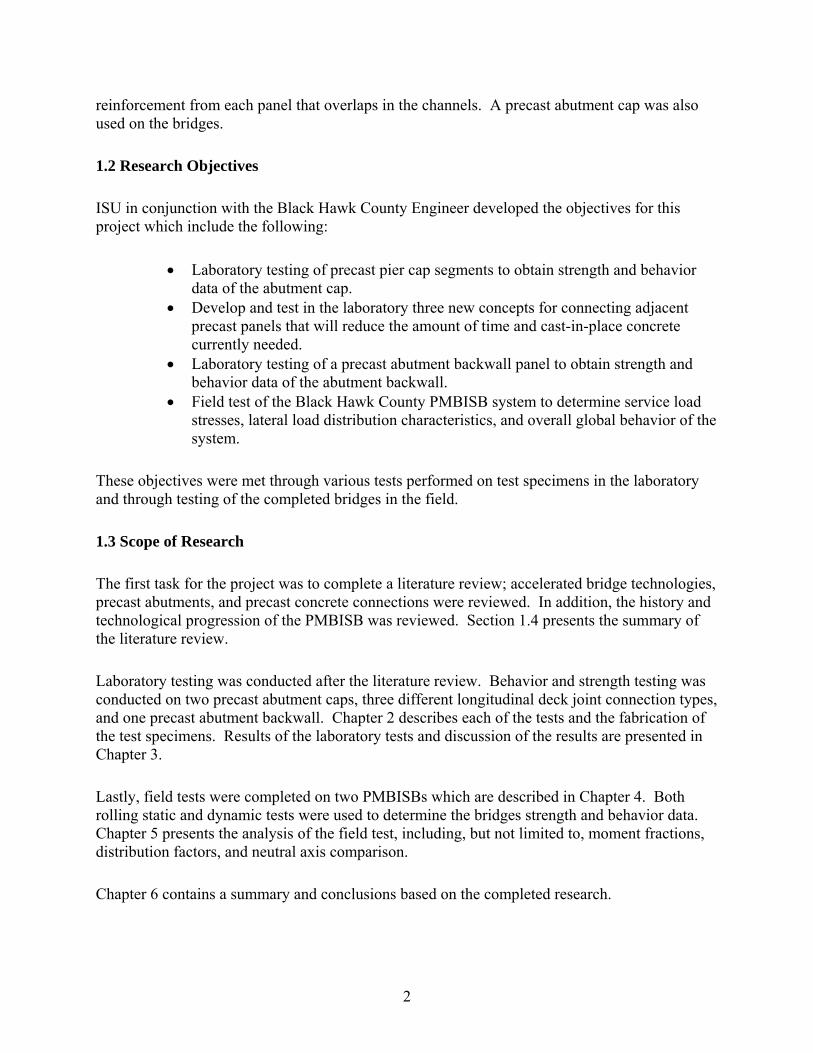
Concrete was placed using the same procedure that was used for the Type 1 Connections. During the placing of the concrete, twelve control cylinders were made using the concrete from the same batch. Before finishing the surface, which was done with a trowel, two anchors were put into the fresh concrete to facilitate movement of the connections in the laboratory. The finished surface of the six specimens, with the anchors in place, is shown in Figure 2.20. Wet burlap and plastic sheets were placed on top of the finished concrete for seven days of curing after which time the burlap, plastic sheets and formwork were removed.

Figure 2.20. Finished concrete and positioned anchors for Type 2 Connection

After curing, the Type 2 Connection specimens were positioned so that the C-channel on one specimen was in contact with the C-channel on an adjacent specimen. Plates (2.5 in. wide x 3/8 in. thick x 15 in. long), were then welded to the top and bottom surfaces of the C-channels. Afterwards, the connections were arranged as shown in Figure 2.21 with plywood formwork at the ends for the closure pour. The concrete used for the closure was not the standard C4 mix, but a high early strength concrete, O-4-S35 BCB, from another concrete pour going on that same day. Nine control cylinders were cast during the placement of the concrete. Finishing was completed with a trowel, followed by covering the concrete with burlap and plastic for a 7 day wet cure.

24

Figure 2.21. Type 2 Connection prepared for closure pour


Type 3 Connection is the same as Type 1 Connection, except for the type of reinforcing that is added to the closure pour area. Instead of two longitudinal bars with additional transverse bars tied into the joint, a length of #4 bar bent into a continuous “S” shape is placed into the joint, supported by the protruding #4 bars, after which, the closure pour is performed shown in Figure 2.22.

Formwork for the Type 3 Connection was assembled into a single form, 96 in. long x 40 in. wide. The forms were uniformly 17 in. tall. The steel forms were oiled to allow cured concrete to easily separate from the concrete. Plywood was again used to separate the forms into sections. Notches were cut into the plywood to allow 1 in. thick x 5 in. tall x 8 ft. long boards to be added to the formwork for the purpose of forming the vertical portion of the closure area. Metal keyways were prepared in the same manner as the keyways for the Type 1 Connections, and were attached to the boards to form the shear key. PVC pipe 18.75 in. in diameter was cut into three 30 in. long pieces, cut in half longitudinally, and centered in the form. Boards (1 in. thick x 25/8 in. tall x 30 in.) were placed on top of the PVC to separate each section. A single exterior tie was used to maintain the 40 in. distance between the sides of the forms.

25

14"

#4's @ 15"

#6's @ 15"5"

CLOSURE AREA

a) Side view

15"

7.50"

7.5"BENT #4 BAR

(PLACED BEFORECLOSURE)

b) Top view


Twelve 18 in. #6 bars and twelve 24.5 in. #4 bars were cut to length. The #4 bars (15 in. on center) were positioned using half-inch holes drilled into the 1 in. x 5 in. board forming the closure area 23/4 in. from the top of the specimen. Since the forms for each side of the connection faced its opposite side, the #4 bars were tied together in the closure area to hold the bars in position. The #6 bars were placed on top of and tied to 11 in. high chairs, positioning the #6 bars 5.5 in. from the top surface. Small blocks of plywood were cut and placed on top of the PVC pipe to maintain the correct depth of the #6 bars over the PVC. The completed formwork for the Type 3 Connection is presented in Figure 2.23.

Concrete was placed and consolidated in a manner similar to that used in the construction of the other two types of connections. During the placing of the concrete, twelve control cylinders were made using the concrete from the truck. After the forms were filled, anchors were placed in the fresh concrete, and finishing was again performed using a trowel. Curing was aided through the use of wet burlap and plastic sheeting, which was removed, along with the forms, after seven days of curing. Three of the freshly trowled specimens are shown in Figure 2.24.

26

Figure 2.23. Completed formwork for Type 3 Connection

Figure 2.24. Finished concrete for Type 3 Connection

Black Hawk County furnished the S-shaped #4 reinforcing bars, previously described. After the two panel segments were positioned facing each other, the 30 in. bent bar sections were tied to the reinforcement protruding into the closure areas. The closure pour was formed similar to the other closure pours. Concrete was placed by hand, consolidated with concrete vibrators, and finished using trowels. Nine control cylinders were cast during the placement of the concrete. After curing for seven days under wet burlap and plastic sheeting, forms were removed. The closure joint in the Type 3 Connection before concrete placement is shown in Figure 2.25.

27

Figure 2.25. Formwork for closure in Type 3 Connection

2.1.3 Test Set-up

Testing of the connection specimens had two goals. The first was to determine the effectiveness of each connection type in transferring load across the joint; the second to determine the ultimate strength of each connection type. To achieve the first goal, service load testing was performed by applying 5 kips in 500 lb. increments at five different locations. As shown in Figure 2.26, LP3 was at the center of the joint. The second goal was met by loading at two locations on either side of the joint and increasing the load until failure occurred (see Figure 2.27). A pin and roller spaced 2’ – 9” apart were chosen for support conditions along the 30 in. longitudinal sides to simulate the longitudinal girders in the deck panels.

LP 3LP 5LP 1

4 SPACES @ 5"512"

LP 2 LP 4

1'-3"

2'-9" 2'-6" a) Side and end views of service load points

b) Photograph of service test at LP 3

Figure 2.26. Typical service load test

28

2'-9"

P/2P/2

8" 1'-5"

a) Ultimate load points

b) Photograph of ultimate load test

Figure 2.27. Typical ultimate load test

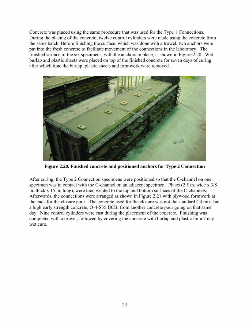
Concrete strain gages and LVDTs were attached to each specimen to determine the strains and deflections that occurred during each test. Strain gages were applied on the top surface of the joint, and on the two sides of the closure pour, as shown in Figure 2.28. A total of 10 strain gages were used for each specimen utilizing the Type 1 and Type 3 Connections. The Type 2 Connections had 13 strain gages, as three strain gages were used to measure strain in the bottom plate as shown in Figure 2.29. Deflections were measured on either side of the joint, so as to be able to determine the differential deflection between the two sides of the joint (see Figure 2.28a).

Specimens were tested when the closure concrete had reached at least 28 day strength, except for the Type 2 Connections, which were tested after 14 days due to high early strength concrete used in the closure area. In the service load tests, specimens were loaded two times, starting at Load Position 1, up to 5000 pounds. Loading was then moved to the next load position, and the process was repeated. A load cell was used to determine the load, and readings were taken at 500 pound intervals. For the service loading, the load was spread over an area of 8 in. by 20 in. in the Type 1 Connection tests. It was determined after testing the Type 1 Connection that a smaller load area would be appropriate for the size of the specimens. Thus, the load was applied

29

over an area of 5 in. by 12 in. for the Type 2 and Type 3 Connections. Areas used for loading in relation to the surface area of the various specimens are shown in Figure 2.30.

16.5"

2.75"

0.75"4.25"6.25"

3.5"

16.5"

DEFLECTION LOCATION1

4 " FROM EDGE

CL

a) Side view b) Top view

Figure 2.28. Strain gage locations in all three connections

18.75"

9"

6"

6"

Bottom view

Figure 2.29. Additional strain gages positioned on bottom plate in Type 2 Connections

30

8"

20"

9.5" (LP2)

15"

30"

33"

40"

CL SUPPORT CL SUPPORT

a) Type 1 Connection service testing load area

5"

20"

9.5" (LP2)

15"

30"

33"

40"

CL SUPPORT CL SUPPORT

b) Type 2 and 3 Connection service testing load area

Figure 2.30. Size of load area on connection surface

After a specimen was loaded at all five load positions, the specimen was set-up for ultimate load testing. To load the specimen at two locations, a beam was used to span the distance between the load points shown in Figure 2.31. By loading the midpoint of the span of the load beam, equal force was applied at each load position. Force was applied until failure of the specimen occurred. Strain and deflection data were recorded at 1000 pound increments. After failure, the broken specimen was examined, removed from the testing area, and then the next specimen was set in place.

31

Figure 2.31. Ultimate load test set-up

2.2 Abutment Backwall

The abutment backwall was precast by Black Hawk County forces, and shipped to the structures laboratory at Iowa State University. The pre-cast backwall is a 14’ – 2” long by 4’ – 3” wide reinforced slab of concrete, designed to support the soil behind the abutment when supported by the flanges of the H-piles in the abutment. The variation in the transverse reinforcement accounts for the increased load with depth due to the lateral earth pressure of the soil: six #4 bars spaced on 12 in. centers for the first 5’ – 6” and 18 #4 bars on 6 in. centers for the remaining 8’ – 6”. Longitudinal reinforcement is provided by four #5 bars that run the entire length of the slab, as shown in Figure 2.32. A drawing of the backwall system in the field, with the backwalls in place between the H-piles is presented in Figure 2.33.

32

9"

9"

4"8"

6"1'6"4'-3"

14'-2"

16 SPACES #4 BARSON 6" CENTERS

5 SPACES #4 BARSON 12" CENTERS

#5 BARS

2"

2"

Figure 2.32. Abutment backwall reinforcement details

54" 54" 54" 54"

~ 6' TO CHANNEL

SOIL

Front view Side view

a) Drawing of backwalls in field

Figure 2.33. Abutment backwalls in the field

33

b) Photograph of backwalls in field

Figure 2.33. Abutment backwalls in the field

In the field, the backwall is restrained laterally at its top edge by the dead weight of the bridge deck acting on the abutment cap, which sits on top of the backwall. At the bottom, lateral restraint is also present due to the soil surrounding the wall. For the laboratory testing, the backwall was modeled as simply supported at the top and bottom of the wall, with the long edges free. For the loading, it was assumed that the front of the wall was not supporting any soil, as would happen due to extreme scouring, and that the back of the wall was supporting a granular soil. Simulation of the field support conditions in the laboratory set-up are presented in Figure 2.34.

RESTRAINTDUE TO SOIL

RESTRAINT DUE TOABUTMENT CAP

Figure 2.34. Correlation of field conditions to the laboratory set-up

34

The backwall spanned a distance of 13’ – 5”, supported by concrete blocks 241/4 in. tall by 163/4 in. wide by 84 in. long. Instrumentation was attached as shown in Figure 2.35 and Figure 2.36: 8 concrete strain gages on top and 4 on the bottom of the backwall, 11 LVDTs on the bottom of the backwall, and 3 steel strain gages on top and 3 on the bottom of each HP10x42, which support the edges of the backwall, for a total of 12 steel gages.

Service testing was performed, both without and with the HP 10x42’s, by applying load at three points on the top of the backwall, shown in Figure 2.38. Starting without the HP10x42’s, the load points were first loaded individually, and then all loaded at different magnitudes of load, to create a triangular load distribution; the ratio of P1 to P2 to P3 was 1 to 3 to 5. After this testing, the HP 10x42’s were installed and positioned so that the backwall was resting on the flanges of the two steel sections as shown in Figure 2.37. Again, the load points were loaded individually and then loaded simultaneously using the same P1/P2/P3 ratio. Neoprene pads were placed under each end of the backwall to maintain the centerline span distance of 13’ - 5” for testing both without and with the HP 10x42’s (see Figure 2.38).

42.5" 42.5"

16"

19"

16"

42.5" 42.5"

1/2"

a) Abutment backwall

47.5" 42.5" 42.5" 47.5"

5"

b) HP 10x42

Strain Gage (Top only)Strain Gage (Top and bottom)

Figure 2.35. Strain gage instrumentation for backwall service test

35

33.5" 42.5" 42.5"

6.5"

9" 33.5"

VERTICAL DEFLECTION TRANSDUCER

9"

6.5"

19"

19"

Figure 2.36. Location of deflection transducers for abutment backwall service load test

HP 10x42

ABUTMENT BACKWALL

HP 10x42

CONCRETE SUPPORTS

a)Plan view of backwall with HP 10’s on edges

b)Photograph of backwall with HP 10’s on edges

Figure 2.37. Backwall supported by 2-HP 10x42s

36

56"56"29" 29"

P1 P2 P3

16.75"

24.25"SLAB LENGTH = 14'-2"

HP LENGTH = 15'-0"

CONCRETE SUPPORT

NEOPRENE

CENTERLINE LENGTH = 13'-5 5/8"

Figure 2.38. Position of loads used in backwall service load tests

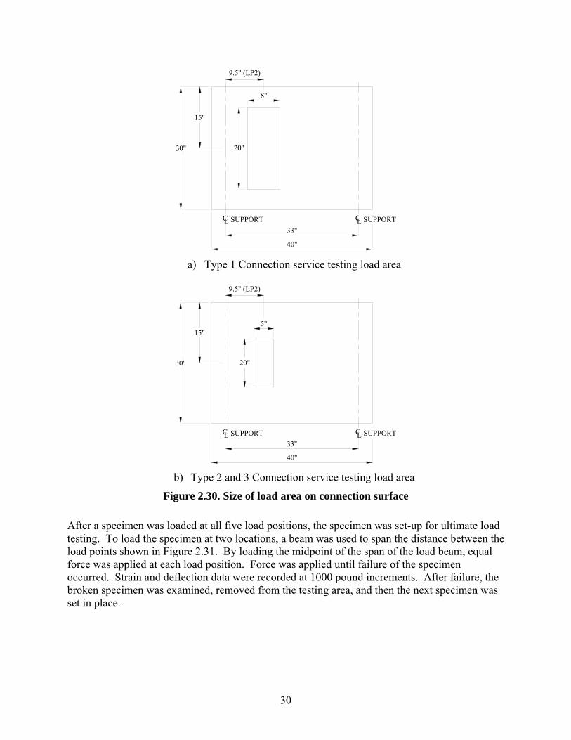
Possible rotation of the piles about their longitudinal axis under the high loads expected during the ultimate load capacity test caused concern about the stability of the system which resulted in slight modifications to the test set-up. To minimize this rotation, steel strap (3 in. x 3/8 in. x 5 ft. long) were bolted to the top and bottom flanges of the HP 10x42’s (see Figure 2.39). Strain gages were mounted on the straps to determine strains in these elements during testing. Additionally, three LVDT’s were attached to the bottom of the flanges and measured any horizontal movement between the steel sections, and four LVDT’s were attached to the bottom face of the backwall at the corners near the concrete supports. The location of the additional instrumentation is shown in Figure 2.39.

The position of the load in the ultimate strength test is 61.4 in. from the bottom of the wall, as shown in Figure 2.40. This location corresponds to the location of the resultant force due to worst case soil loading and five 5-ton axles spaced at 4.25’ on the abutment. Load was applied at this location until the wall was unable to support the load.

33.5" 42.5" 42.5"

6.5"

9" 33.5"

Horizontal Deflection TransducerVertical Deflection TransducerStrain Gage (Top and bottom)

6.5"

9"

31" 43.75" 39"

C OF STEEL HP(HP NOT SHOWN)L

Figure 2.39. Additional instrumentation used in the ultimate strength test of the abutment

backwall

37

25.5"

61.4"

16"

6"

a) Location of load for strength test

b) Photograph of test in progress

Figure 2.40. Strength test of the precast abutment backwall

38

3. LABORATORY TESTING RESULTS

Results from the laboratory testing performed in the ISU structures laboratory are presented in this chapter. First, results from the service level and ultimate strength tests of the abutment caps are presented, followed by the load transfer and strength testing results from the various connection tests. Finally, the precast abutment backwall test results are presented.

3.1 Abutment Cap Test Results

Results from the abutment cap testing described in Section 2.1 are presented in this section. Labeling for the instrumentation used on the W12x65 abutment cap (Cap 1) is shown in Figure 3.1. Gages were identified using the following nomenclature: WXYZ. W refers to the side of the cap and is either N (referring to the north side) or S (referring to the south side). X indicates the material on which the gage is mounted and is C (if the gage is mounted on concrete) or S (if the gage is mounted on steel). Y refers to the six sections (1 through 6) that were instrumented; see Figure 3.1 for the location of these sections. Finally Z is only used with the gages on the concrete and is either T (indicating the gage is on the top concrete surface) or B (indicating the gage is on the bottom concrete surface). For example, NC3T refers to the gage that is on the north side of the cap, for measuring the concrete strains at the top of the concrete, at Section 3. SS2 refers to the gage which is on the south side of the cap, for measuring the steel strains at Section 2. Instrumentation for the W12x26 abutment cap (Cap 2) used the nomenclature that was used for Cap 1, except all gages were on the same side of the cap, eliminating the need for the N/S designation. Also, only five sections were instrumented on Cap 2; see Figure 3.2 for the location of these sections. Pile supports were labeled as shown in Figure 3.1 and Figure 3.2. Note, for both caps, Sections 1, 3, and 5 are at the centerline between the respective supports.

NC1T,SC1T NC2T,SC2T NC3T,SC3T NC4T,SC4T

NC2B,SC2B

NS2,SS2

NC1B,SC1B NC3B,SC3B NC4B,SC4B

NS4,SS4 NS6,SS6NS1,SS1 NS3,SS3 NS5,SS5

A1 B1 C1 D1 E1

Figure 3.1. Identification of strain gages used on Cap 1

C1T

C1B

S1 S2

C2B

S3

C3B

C3T

S4

C4B

S5

C5B

C5T

A2 B2 C2 D2

Figure 3.2. Identification or strain gages used on Cap 2

In the early tests, it was observed that bearing was not achieved on all the piles for the service level testing. This was due to two reasons. Firstly, the cut and grind method used to fabricate the pile sections made it difficult to produce pile sections that were exactly the same length.

39

Secondly, the elevation of the laboratory floor was not constant. Due to these factors, only two piles were supporting each cap during the testing. Despite the fact that the load at each point was increased up to 40 kips, there was never any point were more than two supports were being utilized. Also, the pile sections supporting the caps were not the same for all the tests as the load was moved across the length of the cap. Deflection data from the testing show which piles were supporting the cap for the load at the various load points. Figure 3.3 illustrates which piles were reactive for each load point for Cap 1, while Figure 3.4 illustrates the support conditions for each load point for Cap 2. Presented in Figure 3.5 and Figure 3.6 are the deflection profiles for Cap 1 and Cap 2, respectively. The data presented show the deflection of the abutment cap for a load of 40 kips at each load point; with positive deflections indicating movement downward (towards the floor) and negative deflections indicating movement upward (away from the floor). In each graph, the black triangles indicate the location of the pile supports. It can be seen for Cap 1 that Piles A1 and C1 support the cap for Load Points 1 through 3, and Piles C1 and E1 support the cap for Load Points 4 through 7. For Cap 2, Piles A2 and B2 support the cap for Load Points 1 and 2, while Piles B2 and D2 support the cap for Load Points 3 through 6. The location and magnitude of the maximum deflections (both upward and downward) for both abutment caps are presented in Table 3.1.

Stresses were also calculated from the service tests. The maximum tensile stress in the steel and the maximum compressive stress in the concrete, where they occurred, and the load position for which they occurred are presented in Table 3.2 for both caps. As can be seen, the stresses are very small, especially the concrete with stresses below 0.7 ksi. Figure 3.7 and Figure 3.8 show the steel strain for Cap 1 and Cap 2, respectively. The data presented shows the strain at each steel gage for a load of 40 kips at each load point. It can be seen in these figures that not only are the strains small for steel (corresponding to a stress of 6.5ksi at worst), but that the aforementioned support conditions for the caps are verified.

LP 3LP 2LP 1

A1 C1

a) Load at points LP1, LP2, and LP3

LP 4 LP 5 LP 6 LP 7

C1 E1

b) Load at points LP4, LP5, LP6, and LP7

Figure 3.3. Support conditions for Cap 1 for each load point.

40

LP 2LP 1

A2 B2

a) Load at LP1 and LP2

LP 3 LP 4 LP 5 LP 6

B2 D2

b) Load at LP3, LP4, LP5, and LP6

Figure 3.4. Support conditions for Cap 2 for each load point

Figure 3.5. Deflection profile for Cap 1 for the seven load points used

41

Figure 3.6. Deflection profile for Cap 2 for the six load points used

Table 3.1. Maximum abutment cap deflections

Cap 1 Cap 2 Upward Downward Upward Downward

Magnitude (in.) 0.085 0.043 0.149 0.064 Deflection Location* (in.) 223 28 177 45 Load Point 2 2 1 1

* Measured from left side of abutment cap. See Figure 2.3 and Figure 2.7.

Table 3.2. Abutment cap stresses

Material Specimen Cap 1 Cap 2

Stress (ksi)

Gage

Load Position

Stress (ksi)

Gage

Load Position

Steel (Tensile) 6.1 SS2 LP 2 6.5 S4 LP 4 Concrete (Compressive) 0.68 NC2T LP 2 0.35 CT1 LP 1

42

Figure 3.7. Steel strains for Cap 1 for the seven load points used

Figure 3.8. Steel strains for Cap 2 for the six load points used

43

The uncracked and cracked neutral axes for both caps was calculated by dividing the cross-section into distinct areas, transforming the steel areas into concrete by multiplying the steel area by the modular ratio (Es/Ec), and then using

i

ii

Ay*A

cΣ

Σ=

Where c = neutral axis

iA = ith area, and

iy = distance to the centroid of ith area

Using this equation, the theoretical uncracked neutral axes 9.2 in. from the top of Cap 1 and 7.95 in. from the top of Cap 2 were calculated. The theoretical cracked neutral axes were calculated to be at 8.3 in. and 6.0 in. for Cap 1 and Cap 2, respectively. The neutral axis at Section 2 for both the north and south faces of Cap 1 while the load was at the second load position is shown in Figure 3.9. Note that the top gages are 1 in. below the top of the cap. Both the theoretical cracked and uncracked neutral axis locations are also plotted on this graph. Taking experimental error into account, the laboratory results are in moderately good agreement with the theoretical data points. From Figure 3.9 and Figure 3.10, it appears that there is some eccentricity being developed in the system in that the north face neutral axis is approximately 1 in. lower than the south face neutral axis. A possible explanation for this discrepancy is the uneven bearing on the pile supports or the loading was applied off center.

Figure 3.9. Cap 1 neutral axis at Section 2, Load Position 1, 40 kip load

44

Figure 3.10. Cap 1 neutral axis at Section 2 plotted against load

Using the strain data from Abutment Cap 1, along with calculated properties for the uncracked section, the moment in the section was calculated, and then compared to the moment predicted by beam theory. The theoretical moment was computed twice, once assuming the span length to be the support centerline distance (4.5 ft.), and the second time assuming the span length to be the clear distance between the supports (3.67 ft.). These moments are presented in Table 3.3, and show good agreement between the calculated moments and the clear span moments.

Table 3.3. Abutment Cap 1 moment comparison (calculated at Section 2)

Calculated Moments Load

(at LP 1) Based on Center

Line Length Based on Clear

Span Length Based on

Strain Data (kips) (k-ft) (k-ft) (k-ft)

20 15.0 10.8 11.1 40 30.0 21.7 22.5

The neutral axis calculated from the service testing of Cap 2 and also the theoretical cracked and uncracked axes locations are presented in Figure 3.11. The lines were drawn using the data from the first and second load positions, using the top concrete strain gage and the steel gage at Section 1. Both the theoretical cracked and uncracked neutral axis locations are plotted on the graph (6.04 in. and 7.95 in. from the top of the cap, respectively), as can be seen the experimental axes are within experimental error of the uncracked axis.

45

Figure 3.11. Cap 2 neutral axis at Section 1, Load Positions 1 and 2, at 40 kips

As for Cap 1, moments were calculated for Abutment Cap 2 using the strain data from Section 1 and assuming uncracked section properties. Theoretical moments were computed using beam theory, once based on a centerline span length (5.5 ft.) and again assuming a clear span length (4.67 ft.). These values are presented in Table 3.4; again, the theoretical and calculated moments are in good agreement. Of particular interest is how the span length appears to increase due to higher load. This means that the cap was resting on the corners of the supports initially, but bearing was eventually achieved over the length of the support. Since the moments calculated from the strain data for both caps are in such good agreement with the moments predicted by classical analysis, use of beam theory is acceptable for analysis and design of the caps.

Table 3.4. Abutment Cap 2 moment comparison (calculated at Section 1)

Calculated Moments Load

(at LP I) Based on Center

Line Length Based on Clear

Span Length Based on

Strain Data (kips) (k-ft) (k-ft) (k-ft)

20 16.3 12.1 13.0 40 32.5 24.2 31.7

Both abutment caps were tested to determine their maximum positive moment capacity, and Cap 1 was also tested to determine maximum negative capacity. Cap 1 did not experience failure during the positive capacity test as the limit of the load frame was reached. The threshold for failure was considered to be the point at which load could no longer be sustained by the caps. Load-deflection curves for the positive moment capacity tests for Cap 1 and Cap 2 are presented in Figure 3.12. Notice that the curve for Cap 1 only starts to show non-linear behavior before the test ended (capacity of load system reached) and that the curve for test 2 shows a traditional ductile failure. Cap 1 supported 175 kip, which corresponds to a moment of 765 kip-ft, and

46

deflected 0.87 in. before the test was terminated, while Cap 2 failed when a load of 120 kip, corresponding to a moment of 465 kip-ft, was applied and a deflection of 1.08 in. occurred.

Cap 2 was not tested for negative moment capacity due to the damage sustained during the positive capacity test. The load-deflection curve for the negative moment capacity test for Cap 1 is shown in Figure 3.13. As is clearly seen, Cap 1 experienced a ductile failure at 97 kips, which induced a moment of 363 kip-ft in, deflecting 2.1 in. Factored experimental moment capacities for the caps, along with their factored theoretical capacities (determined from strain compatibility), are presented in Table 3.5. The design moment for the caps for both positive and negative bending is 156 kip-ft. Both caps exceed the positive capacity called for by the designer, while Cap 1 exceeded the capacity required for negative moment capacity. While not tested for negative moment capacity, Cap 2 should have more than enough capacity to meet the moment demand required of it. This can be deduced from the excellent performance of Cap 1 coupled with the fact that Cap 2 has more reinforcing steel than Cap 1 during negative bending. According to Black Hawk County, Cap 2 is much more cost effective than Cap 1, as Cap 2 saves approximately $1000 per abutment cap in material cost. Due to adequate moment capacity and significant cost savings, Cap 2 should be used for future PMBISB projects.

Figure 3.12. Plot of load vs. deflection for positive capacity tests of caps

47

Figure 3.13. Plot of load vs. deflection for negative capacity test of Cap 1

Table 3.5. Abutment cap capacities

Experimental Capacities (kip-ft)

Mn+ (factored: φ = 0.9) Mn

- (factored: φ = 0.9)

Laboratory

Strain Compatability

Laboratory

Strain Compatability

Cap 1 765+* 752 327 344 Cap 2 419 356 - 272 * Testing halted before failure because limit of load frame reached Note: Factored Design Demand (Mu+ and Mu-) is 156 kip-ft

3.2 Connection Test Results

Results from the connection detail testing described in Chapter 2.2 are presented in this section. Proposed details were tested for response to service level loading conditions and ultimate loading conditions for the purpose of determining a preferred connection detail. In this report, the Type 1 detail is considered the baseline as the detail had already been used in the construction of a PMBISB.

Results from the service level testing show that all three connection details were able to transmit the 5 kip load across the joint. Figure 3.14, Figure 3.15, and Figure 3.16 show deflections for each connection type for both the left and right sides of the specimen. In these figures, the service loading started on the left side, and moved to the right side. For the Type 1 and Type 3

48

Connections, the side of the specimen that is carrying the load deflects more than the other side, as is expected since there is no positive connection between the instrumented areas (see Figure 2.28 for deflection instrumentation locations). The Type 2 Connection deflections show continuity between the two sides of the specimen. This was expected as the welded plates create a positive connection in the Type 2 Connection. The instrumentation labeling for the concrete gages on the top surface of the specimens is shown in Figure 3.17. Table 3.6 presents the highest compressive strains that occurred in these strain gages for all three connection types.

Figure 3.14. Type 1 Connection service deflections


49


16.5"

2.75"

16.5"

CL

DIRECTIONLOAD MOVEDACROSS JOINT

II-B II-A

I-B I-A

Figure 3.17. Labeling for top concrete strain gages

Table 3.6. Maximum compressive concrete strains on connections

Connection Strain (MII) Gage Type 1 44 IB Type 2 66 IIA Type 3 42 IB

50

To determine the preferred connection type, the cost, constructability, and capacity of each connection type was compared to the others. Differences in cost between the connections are from the differences in detailing. Costs to construct a single specimen of each connection type are presented in Table 3.7. These costs are based on material prices paid by the ISU Structures Laboratory. Concrete cost is the same between all the connections because there is no difference in volume of concrete when both the block units and the closure area are considered. Type 2 is much more expensive than either the Type 1 or Type 3 Connections because of the cost of the structural steel pieces needed for the Type 2 detail.

Table 3.7. Single specimen material cost

Material Cost of a Single Specimen ($)

Type 1 Detail

Type 2 Detail

Type 3 Detail

Concrete 22.44 22.44 22.44 #4 Bar 4.70 - 4.06 #6 Bar 4.23 4.26 4.23

C-Channel - 12.56 - Steel Plate - 4.18 -

Total 31.37 43.44 30.73

Constructability of a detail is a criterion for determining the preferred connection as more constructible details will generally result in faster build times, ultimately accelerating the construction process. Both the Type 1 and Type 3 details are easily constructed, especially in the field since #4 reinforcing bar is placed into the closure area. The Type 2 detail is more difficult to construct in the field due to the need to perform overheard welding in the field. Since many bridges are built to traverse waterways, moving the welder and the welding equipment into position can be very difficult. For these reasons, both the Type 1 and Type 3 details are preferred from the constructability standpoint.

A comparison of the ultimate strength of the connections was the last criteria for selection of the preferred detail. Load was applied on both sides (see Figure 2.27) of the joint until failure occurred. Specimens were considered failed when deflection increased without a corresponding increase in load. The load at which each specimen failed is presented in Table 3.8. All the results were normalized to the concrete strength of the Type 1 detail. The values given correspond to the load on one side of the joint (refer back to Figure 2.27), meaning the total load supported by each specimen is twice the value in the table. Deflections at failure for each specimen are also presented in Table 3.8.

As previously noted, the Type 1 Connection was used as a baseline for comparison. By far, the Type 2 detail supported the most load, most likely due to the fact that it utilizes a positive connection between the two sides. The Type 3 detail did not perform as well as anticipated, supporting noticeably less load than the Type 1 detail. Using strength considerations, the Type 2 detail is preferred, followed by the Type 1 detail.

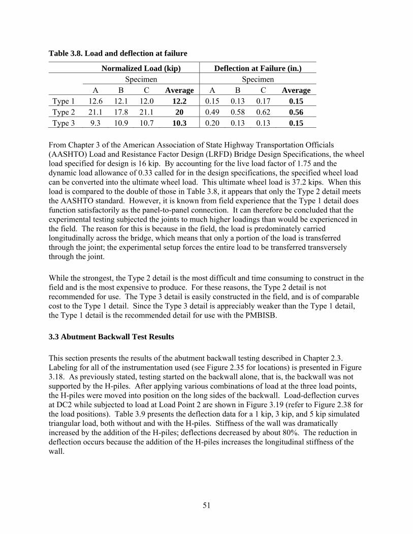
51

Table 3.8. Load and deflection at failure

Normalized Load (kip) Deflection at Failure (in.) Specimen Specimen A B C Average A B C Average Type 1 12.6 12.1 12.0 12.2 0.15 0.13 0.17 0.15 Type 2 21.1 17.8 21.1 20 0.49 0.58 0.62 0.56 Type 3 9.3 10.9 10.7 10.3 0.20 0.13 0.13 0.15

From Chapter 3 of the American Association of State Highway Transportation Officials (AASHTO) Load and Resistance Factor Design (LRFD) Bridge Design Specifications, the wheel load specified for design is 16 kip. By accounting for the live load factor of 1.75 and the dynamic load allowance of 0.33 called for in the design specifications, the specified wheel load can be converted into the ultimate wheel load. This ultimate wheel load is 37.2 kips. When this load is compared to the double of those in Table 3.8, it appears that only the Type 2 detail meets the AASHTO standard. However, it is known from field experience that the Type 1 detail does function satisfactorily as the panel-to-panel connection. It can therefore be concluded that the experimental testing subjected the joints to much higher loadings than would be experienced in the field. The reason for this is because in the field, the load is predominately carried longitudinally across the bridge, which means that only a portion of the load is transferred through the joint; the experimental setup forces the entire load to be transferred transversely through the joint.

While the strongest, the Type 2 detail is the most difficult and time consuming to construct in the field and is the most expensive to produce. For these reasons, the Type 2 detail is not recommended for use. The Type 3 detail is easily constructed in the field, and is of comparable cost to the Type 1 detail. Since the Type 3 detail is appreciably weaker than the Type 1 detail, the Type 1 detail is the recommended detail for use with the PMBISB.

3.3 Abutment Backwall Test Results

This section presents the results of the abutment backwall testing described in Chapter 2.3. Labeling for all of the instrumentation used (see Figure 2.35 for locations) is presented in Figure 3.18. As previously stated, testing started on the backwall alone, that is, the backwall was not supported by the H-piles. After applying various combinations of load at the three load points, the H-piles were moved into position on the long sides of the backwall. Load-deflection curves at DC2 while subjected to load at Load Point 2 are shown in Figure 3.19 (refer to Figure 2.38 for the load positions). Table 3.9 presents the deflection data for a 1 kip, 3 kip, and 5 kip simulated triangular load, both without and with the H-piles. Stiffness of the wall was dramatically increased by the addition of the H-piles; deflections decreased by about 80%. The reduction in deflection occurs because the addition of the H-piles increases the longitudinal stiffness of the wall.

52

HP 10x42

TMN

TN1

TS1

DN1

DC1

DS1

DCW

DN2

TN2, BN2

DC2

TS2, BS2

DS2TMS

DN3

TN3, BN3

DC3

TS3, BS3

DS3

DCE

SN1,SS1 SN2,SS2 SN3,SS3

DNW DNE

DSSDSW

ST1/SB1 ST2/SB2 ST3/SB3

DD1 DD2 DD3

HORIZONTAL DEFLECTION TRANSDUCERSTRAIN GAGE (TOP ONLY) VERTICAL DEFLECTION TRANSDUCERSTRAIN GAGE (TOP AND BOTTOM)

Figure 3.18. Labels for the abutment backwall instrumentation

Figure 3.19. Load-deflection curves for Load Point 2 at LVDT DC2

Table 3.9. Deflections for 1 kip, 3 kip, and 5 kip simulated triangular load

Measured Deflection (in.) DC1 DC2 DC3

Without Beams 0.087 0.146 0.098 With Beams 0.014 0.022 0.020 % Change 84.3% 84.7% 79.3%

53

Changes in the longitudinal strains (gages TMN, TMS, SN2, and SS2) at the edge of the backwall are presented in Table 3.10. Not surprisingly, the concrete strain is reduced once the piles are installed, and the piles experience strains from the applied load. As can be seen, the load on the north side of the backwall was almost completely carried by the steel H-pile. Concrete on the south side of the backwall did not experience the same level of reduction as the concrete on the north side did. It was observed during the installation of the H-piles that the wall did not rest perfectly on the flanges of the H-piles, which accounts for the seemingly ‘extra’ strain in the concrete on the south side of the backwall.

Table 3.10. Changing strain on the exterior of the abutment backwall due to H-piles

Exterior Midspan Strains (MII) TMN TMS SN2 SS2

Without Beams -69 -70 - - With Beams -2 -18 -63 -44

AASHTO recommends that horizontal abutment movements should be less than 1.5 in. When the wall was subjected to a triangular load pattern of 5 kip, 15 kip, and 25 kip, the maximum deflection was only 0.17 in., which is well below the recommended value. The load pattern applied corresponds to a clay backfill, under a worst-case lateral earth pressure condition.

An ultimate load test was performed by loading the slab at a single point 61.4 in. from the bottom of the wall. The slab was damaged during the first attempt when the spliced H-pile failed; the quality of the weld was poor, and the tension flange ruptured. At the time of the failure, the system was carrying 80 kips. The H-pile was repaired by welding plates to the exterior of each flange, and using a full-penetration weld along the web; the splice repair is shown in Figure 3.20.

Figure 3.20. Repaired H-pile splice

54

After the repair, the test was performed again, and the slab was still able to resist a point load of 100 kips. The load-deflection curves at DC2, both before and after the H-pile break, are shown in Figure 3.21. The failed backwall specimen is shown in Figure 3.22; the pattern of the cracking suggests that punching shear was the mode of failure. During the strength testing, the stress induced in the steel straps was less that 2.7 ksi for the top straps and less than 1.1 ksi for the bottom straps. The expected resultant load from both a 5-axle, 10 tons per axle truck over the abutment and the lateral earth pressure from an undrained clay under worst-case conditions is approximately 63 kips. Even in its weakened state, the backwall system provided a factor of safety of 1.6 against failure.

Figure 3.21. Load-deflection curves for strength testing at DC2 before and after HP break

Figure 3.22. Failed abutment backwall specimen

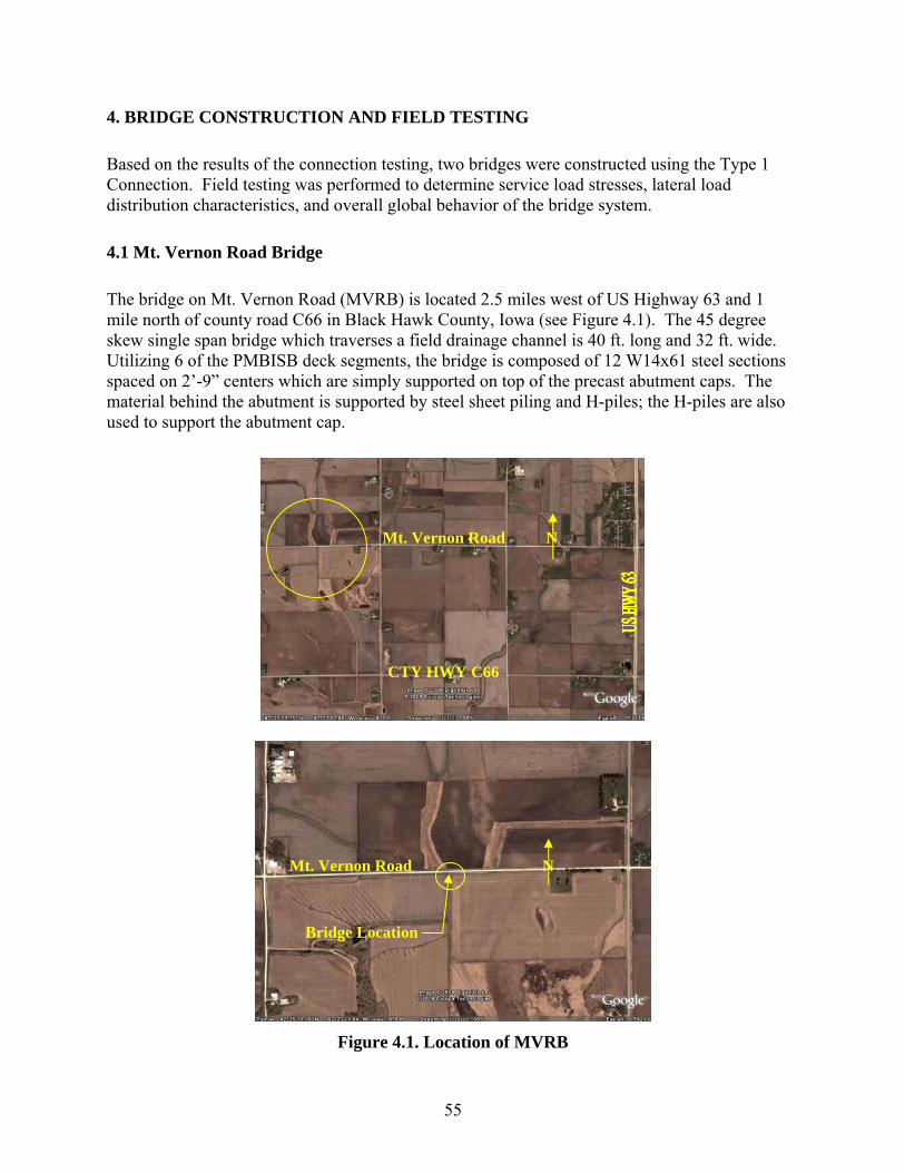
55

4. BRIDGE CONSTRUCTION AND FIELD TESTING

Based on the results of the connection testing, two bridges were constructed using the Type 1 Connection. Field testing was performed to determine service load stresses, lateral load distribution characteristics, and overall global behavior of the bridge system.

4.1 Mt. Vernon Road Bridge

The bridge on Mt. Vernon Road (MVRB) is located 2.5 miles west of US Highway 63 and 1 mile north of county road C66 in Black Hawk County, Iowa (see Figure 4.1). The 45 degree skew single span bridge which traverses a field drainage channel is 40 ft. long and 32 ft. wide. Utilizing 6 of the PMBISB deck segments, the bridge is composed of 12 W14x61 steel sections spaced on 2’-9” centers which are simply supported on top of the precast abutment caps. The material behind the abutment is supported by steel sheet piling and H-piles; the H-piles are also used to support the abutment cap.

Figure 4.1. Location of MVRB

Bridge Location

CTY HWY C66

Mt. Vernon Road N

Mt. Vernon Road N

56

Each 5.5 ft. wide interior deck panel has two W14x61 sections connected by transverse steel reinforcing bar and concrete. Holes (1.25 in. diameter) are torched into the web of the W14’s on 3 in. centers and 2.25 in. from the top flange, and #6 bars are placed into the holes at 15 in. intervals. Number 4 reinforcing bars (6’ – 3” in length) are positioned transversely on the top flange of the W14 on 15 in. centers. Arches between the steel sections and at the edges of the panel are created with 18.7 in. diameter PVC pipe. Concrete was placed after the reinforcing steel and PVC were positioned; a typical cross-section of the unit is shown in Figure 4.2.

Construction of the MVRB took place in June, 2006. First, nine HP10x42 H-piles were driven at each abutment, followed by driving steel sheet piling behind the H-piles. The precast abutment caps were placed on top of the H-piles (Figure 4.3), and 1-1/2 in. crushed limestone was used for fill behind the sheet pile abutments.

7"

3"

2"

#6 BARS

#4 BARS

1'-5"

5'-6"

#6 BARS

9.375"

Figure 4.2. Typical cross-section of the PMBISB

Figure 4.3. Abutment cap on H-piles

During the first day of superstructure construction, deck panels were transported to the site one at a time, using a semi-tractor and flatbed trailer. A crane was used to lift each panel from the trailer and place it on three steel beams that temporarily spanned the distance between the abutments as shown in Figure 4.4. Once the panel was on the beams, rigging from a crane on the

57

opposite abutment was attached to the panel, and both cranes were used to place the panels in their final positions (see Figure 4.5). Once three panels had been placed, the temporary beams were removed, and subsequent panels were then placed temporarily on top of the previously set deck panels to allow the second crane to attach to the lift points on the panels as shown in Figure 4.6. While the semi was in route for another panel, reinforcing bars were placed into the connection area between the panels as described in Section 3.2.1.1.

The second day of superstructure construction began by torching off the lifting hoops and using PVC pipe for formwork to prevent concrete from flowing through larger than anticipated gaps between panels (see Figure 4.7). Concrete was then placed in the closure areas between the panels (see Figure 4.8). Shovels, a wheelbarrow, and an electric concrete vibrator were used to place the concrete, while trowels were used to finish the concrete. The surface of the concrete was roughened, and a curing agent was applied. A view of the finished concrete deck is shown in Figure 4.9. Guardrails were attached the next day, and the bridge was opened one week later. Thus, it took nine days to complete the bridge after the substructure was in place.

Figure 4.4. Temporary beams for setting panels

Figure 4.5. Using two cranes to position a deck panel

58

Figure 4.6. Setting panel on superstructure

Figure 4.7. PVC form used in the location of a gap between the concrete panels

Figure 4.8. Closure concrete placement

59

Figure 4.9. View of completed bridge

A field test was performed on MVRB to quantify the structural behavior with particular interest in the resulting stresses, deflections, and lateral load distribution. Instrumentation was applied to the bridge to measure mid span deflection and strains (at the abutments, quarter span, and mid span). Load was applied to the bridge by a loaded tandem axle dump truck provided by Black Hawk County. Axle spacing and weight of the test vehicle (total weight = 55.8 kips) are presented in Figure 4.10; an assumption was made that the measured tandem weight was evenly distributed between the two axles. For the testing, 26 BDI’s and 12 DCDT’s were attached to the bridge and five load lanes were marked out on the bridge deck. A detailed layout of the instrumentation and the loading lanes is presented in .

Figure 4.10. Wheel and load configuration for MVRB test vehicle

The bridge was subjected to a series of rolling and dynamic tests to maximize the desired effects; rolling tests consisted of the test vehicle crossing the bridge in each of the test lanes at approximately 2 mph. The truck went across each test lane twice, for a total of ten static tests. For the dynamic tests, the test vehicle traveled across the bridge centered transversely; twice at 15 mph and twice at 25 mph for a total of 4 dynamic tests. Results of the field testing for the MVRB are presented in Section 5.1.

60

30.0"

98.2"

112.1"

112.1"

98.2"

43.5"

31.75'WEST ABUTMENT

1/4 SPAN

MIDSPAN

3/4 SPAN

EAST ABUTMENT

G1G12

BDI, BOTTOM

DCDTBDI ON GUARDRAIL

N

BDI, TOP & BOTTOM

67.5"

108.0"

190.5"

313.5"

273.0"

LOADING LANES

Figure 4.11. Instrumentation and loading lane layout for MVRB

61

4.2 Marquis Road Bridge

Located north-east of Waterloo, 2 miles north of County Road C57 and 4.25 miles east of US Highway 63 (see Figure 4.12), the Marquis Road Bridge (MRB) is 39 ft. long and 26.5 ft. wide, with no skew. A total of five precast panels were used for the bridge, constructed in the manner described in Section 4.1. The panels were placed on top of the precast abutment caps which are supported by driven HP10x42 steel sections. Driven sheet piling behind the H-piles was used to support the soil behind the abutment.

Figure 4.12. Location of MRB

Bridge Location

CTY HWY C57 N

Marquis Road

Marquis Road N

62

On August 30, 2007, the precast abutment caps were placed on top of the driven H-piles by using a crane, shown in Figure 4.13. The superstructure was constructed in the same manner as the MVRB, on September 10 and 11. During the first day, a semi-tractor and trailer was used to transport the panels to the construction site, and two cranes were used to place the panels in their final position. Because of rain on the first day, placement of the reinforcing steel in the closure joint was postponed until the second day. While the steel was being placed, the steel lifting hoops were torched off the panels. After those tasks were completed, concrete was brought to the site via a concrete truck, and was placed in the closure area using a concrete bucket, shown in Figure 4.14. Concrete being placed in the closure area is shown in Figure 4.15. After all the closure joints had been filled, the surface of the concrete was roughened and a curing agent was applied. Figure 4.16 shows the finished concrete bridge deck. As with the MVRB, guardrails were installed the next day and the bridge opened one week later. Again, it took nine days to complete the bridge after the substructure was in place.

Figure 4.13. Placement of the precast abutment cap for the MRB

Figure 4.14. Using concrete bucket for placement

63

Figure 4.15. Concrete in closure area

Figure 4.16. View of the completed bridge deck

A field test was performed on the MRB to quantify its structural behavior. Instrumentation was applied to the bridge to measure mid-span deflections and strains (at the abutments, quarter span, and mid span) for the purpose of determining live load stresses, deflections, and determining the lateral load distribution from a truck load. Load was applied to the bridge using a loaded tandem axle dump truck provided by Black Hawk County. Axle spacing and weight of the test vehicle (total weight = 55.6 kips) are presented in Figure 4.17; an assumption was made that the measured tandem weight was evenly distributed between the two axles. The truck had the same geometry as the truck for the MVRB, but with a different weight. For the testing, 30 BDI’s and 14 DCDT’s were attached to the bridge and three load lanes were marked out on the bridge deck. A detailed layout of the instrumentation and the loading lanes is presented in Figure 4.18.

Pseudo-static testing was performed by marking three different lanes on the bridge, and then having the truck move across the bridge, in each lane, at approximately 2 miles per hour. The truck went across each test lane twice, for a total of ten static tests. For the dynamic tests, the test vehicle traveled across the bridge centered transversely; twice at 15 mph and twice at 25 miles per hour for a total of 4 dynamic tests. Results of the testing of the Marquis Road Bridge are presented in Section 5.2.

64

87" 72"

182" 54"

18.6 kips 18.5 kips 18.5 kips Figure 4.17. Wheel and load configuration for MRB test vehicle

Figure 4.18. Instrumentation and loading lane layout for MRB

65

5. BRIDGE FIELD TESTING RESULTS

5.2 Mt. Vernon Road Bridge

The bridge on Mt. Vernon Road was tested as described in Section 4.1. The 10 rolling tests will be referred to as Test X.Y, where X is the lane number (X = 1, 2, 3, 4, 5), and Y designates whether it was the first crossing in that lane (Y=1), or the second (Y=2). A significant amount of strain and deflection data was collected during each of the individual tests. The data were reduced by plotting the midspan tensile strains versus time and determining the time when maximum strains occurred. As an example, the measured midspan strains for Test 4.1 are presented in Figure 5.1. For this case, the maximum effect occurred at approximately 20.6 seconds on Girder 11; hence all data readings taken at this selected time were used to evaluate the bridge behavior for this test. The data marks introduced during the rolling test were used to calculate the truck’s location at the maximum strain effect. The calculated position of the rear tandem axle is 56 ½ in. before the bridge’s midspan at the time of maximum strain effect (197 in. from the centerline of the East Abutment). As seen in Figure 5.1, the maximum strains in each girder do not occur at the same time; this is due to the skew of the bridge. The mispan strains for Test 5.1 are also presented in Figure 5.2 and also show the effect of the skew for when the maximum strains occur. For all test lanes, it was found that the maximum 1/4 span strains were always less than maximum midspan strains.

Figure 5.1. Midspan strain history for Test 4.1

The maximum midspan tensile and compressive strains due to the field tests were converted to a stress (assuming Es=29,000 ksi and Ec=4,030 ksi). The maximum tensile stress in the steel was 2.5 ksi and occurred during Test 5.1 in Girder 12, while the maximum compressive stress in the concrete was 0.27 ksi, also occurring during Test 5.1. Allowable stress for the steel used in the design of the panel was 27.5 ksi (.55fy), and for the concrete was 2 ksi (0.4f’c). Since the test vehicle isn’t as heavy as the AASHTO vehicle (72 kips), the stresses need to be factored

66

accordingly in order to compare to the AASHTO allowable stresses. After factoring, the maximum steel stress is 3.2 ksi and the maximum concrete stress is 0.35 ksi. Dead load stresses were determined from the BHC design spreadsheet, which shows the steel stress as 9.4 ksi and the concrete stress as 0.45 ksi. Therefore, the total steel stress is 11.9 ksi, and the total concrete stress is 0.69 ksi, which are much lower than what is allowed. Thus, the MVRB meets the AASHTO design criteria.

Figure 5.2. Midspan strain history for Test 5.1

The location of the bridge’s neutral axis was determined for each test by assuming a linear strain profile through the cross section between the compressive strain values on the deck surface and the tensile strain values on the beam’s bottom flange. The experimental neutral axes for Test 4.1 are presented graphically in Figure 5.3, resulting in a range of neutral axes values from 7.15 to 7.74 in. below the concrete deck. The experimental neutral axes for Test 5.1 are presented in Figure 5.4. Also, shown are the theoretical gross and cracked transformed neutral axes; gross neutral axes for the interior and exterior girders are 7.65 and 8.23 in., respectively, while cracked experimental values for interior and exterior girders are 5.9 and 6.35 in., respectively.

Theoretical neutral axes were calculated for the interior and exterior longitudinal beams for both uncracked and cracked transformed sections. The section properties of the interior and exterior beams were determined by first transforming concrete properties to steel properties by applying a modular ratio of 7, which is calculated by dividing Young’s modulus for steel by Young’s modulus for concrete. The neutral axes of the uncracked interior and exterior sections were computed using Equation 5.1.

∑∑ ∗

=i

ii

AyA

c Equation 5.1

Where: c = neutral axis from top of the section, in. Ai = Transformed area of the ith part, in2

iy = Neutral axis of the ith part from the top of the section, in.

67

Figure 5.3. Test 4.1 neutral axes


68

The theoretical cracked neutral axis was developed by equating the internal compressive and tensile forces. For the cracked sections, all concrete below the neutral axis was assumed to be ineffective in resisting flexure. A linear strain profile was assumed and Hooke’s Law was applied to relate strains to stresses that were then converted to equivalent forces. Forces above the assumed neutral axis are compressive while forces below the assumed neutral axis are tensile. Equilibrium of the resulting horizontal forces was obtained by adjusting the zero strain depth (neutral axis) to balance the forces producing the position of the cracked neutral axis. The cracked neutral axes are approximately 2 in. higher than the uncracked neutral axes.

The theoretical neutral axes results, listed in Table 5.1, are distances from the top of the cross-section. The cracked and uncracked midspan neutral axes of the theoretical interior longitudinal beam bracket the experimental midspan neutral axes results (also shown in Table 5.1). Consequently, these results provide evidence that the bridge has an effective cross-section bounded by the fully cracked and gross section; the bridge behaves as if partially cracked. This behavior was observed for all five test lanes.

Table 5.1. Depth to neutral axes during Tests 4.1 and 5.1

Neutral Axis Depth (in.)

Interior Girder

Exterior Girder

Experimental Test 4.1 7.74 7.15 Experimental Test 5.1 7.68 7.12 Theoretical Uncracked 7.65 8.23 Theoretical Cracked 5.9 6.35

The strains recorded in the thrie beam guard rails were also evaluated. In Figure 5.5, the strains in the south and north guard rails are plotted versus time for the truck in loading Lane 4. In this figure, compressive strains close to 40 microstrain occur in the south guardrail, indicating that the guard rail contributes to the flexural resistance of the PMBISB system. The contribution of the guard rails varies, depending on the location of the truck. The contribution increased when the truck was closer to the rails, and decreased as the truck moved away from the rails.

Girder strains at the abutments were evaluated to determine if end restraint was present. In Figure 5.6, the strains at the abutments in Girders 7, 9, 10, and 12 recorded during Test 4.1 are plotted versus time. The maximum compressive strains occurring in either abutment were less than 10 microstrain. Since compressive strains are recorded, the instrumentation is located in a negative moment region, indicating the ends are not purely simply supported. The area of the deck panels that rests on the abutment cap creates a semi-rigid condition at the abutments.

Deflections at the midspan were taken at the same time as the maximum midspan strains. The deflections were used to develop transverse midspan profiles. The transverse midspan deflections resulting from all five test lanes are presented in Figure 5.7. It can be seen that for a single truck, most of the load is carried in a single lane.

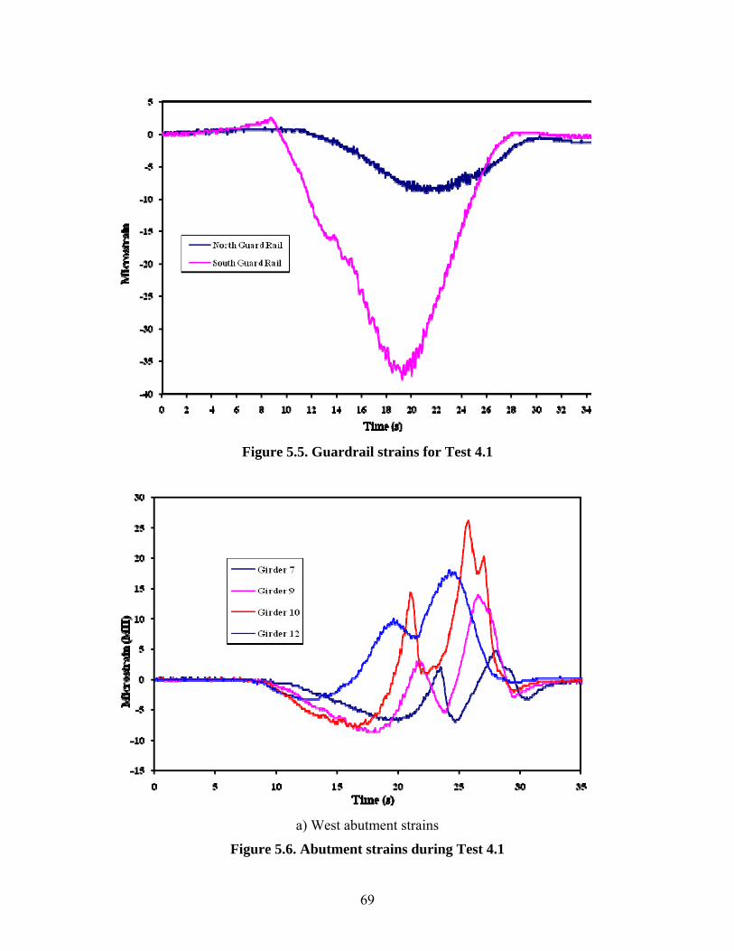
69

Figure 5.5. Guardrail strains for Test 4.1

a) West abutment strains

Figure 5.6. Abutment strains during Test 4.1

70

b) East abutment strains


Figure 5.7. Midspan displacement profiles for all five test lanes

71

The serviceability of the bridge was evaluated by examining the maximum recorded deflections. The maximum midspan deflection was 0.179 in. and occurred during Test 1.1. Adjusting this value to account for the AASHTO design truck results in a maximum midspan deflection of 0.231 in. The suggested serviceability limit from the AASHTO LRFD Bridge Design Specifications was 0.596 in. (Span/800), which is 2.6 times greater than the adjusted value.

Displacements were also measured between adjacent panels at the centerline joint (between the third and fourth panels, see Figure 4.11). Differential displacement between these panels is shown in Figure 5.8. The maximum difference is only 0.007 in., which is 4% of the maximum amount of displacement along the centerline. Thus, the new connection detail is effective in transferring load across the bridge deck.

Figure 5.8. Differential displacements along centerline joint

Load fractions and the load distributions determined from the testing of the Mt. Vernon Road Bridge are presented in Figure 5.9 and Figure 5.10, respectively. Also shown are the fractions and distribution factors as calculated from the AASTHO LRFD Bridge Design Specifications and the factor used for the design. Note that the factors used for design were based on the AASHTO Standard Specification for Bride Design (AASHTO 2002). The experimental fractions and factors were below those used for design, and those recommended by current AASHTO standards (AASHTO 2006).

72

Figure 5.9. Single lane DF from deflections

Figure 5.10. Two lane DF from deflections

73

The load fractions for each lane were calculated as shown in Equation 5.2:

∑δ

δ=

i

i

LF Equation 5.2

Where: iδ is the deflection the ith girder

Equation 5.2 assumes that the moment of inertia for each girder is the same. For the PMBISB system, the exterior girders have a larger moment of inertia than the interior girders. It is for this reason that the load fractions calculated are approximate.

Distribution factors were calculated from the experimental data by using superposition to add the load fractions for two lanes together. Lanes were only added together if the transverse position of the truck for the lanes did not overlap.

AASHTO distribution factors were calculated for both a single loaded lane (Equation 5.3) and two loaded lanes (Equation 5.4). These equations were taken from AASHTO LRFD Bridge Design Specification Article 4.6.2.2. Equation 6.3 has the multi-presence factor included. Due to the fact that for the field testing there was only one vehicle on the bridge, the values obtained using Equation 5.3 were divided by 1.2.

1.0

3s

g3.0.4.0

Lt12K

LS

14S06.0 ⎟⎟

⎠

⎞⎜⎜⎝

⎛⎟⎠⎞

⎜⎝⎛

⎟⎠⎞

⎜⎝⎛+ Equation 5.3

1.0

3s

g2.06.0

Lt12K

LS

5.9S075.0 ⎟⎟

⎠

⎞⎜⎜⎝

⎛⎟⎠⎞

⎜⎝⎛

⎟⎠⎞

⎜⎝⎛+ Equation 5.4

Where: S = spacing between girders, ft L = span length of the bridge, ft Kg = longitudinal stiffness parameter, in4 ts = thickness of the slab, in.

It is important to note that AASHTO only allows the use of these formulas if S is greater than 3.5 ft, but less than 16 ft. Since S for the MVRB is only 2.75 ft, strictly speaking, the AASHTO LRFD factors do not apply. However, as is seen in Figure 5.9 and Figure 5.10, the AASHTO LRFD factors are not overwhelmingly conservative, especially for the single lane loading.

The design factors were calculated as stated by the AASHTO Standard Specification for Bridge Design (AASHTO 2002). Equation 5.5 is for a single lane loading, and Equation 5.6 is for

74

loading in two or more lanes. These equations produce factors for wheel loads, not truck loads. As such, the factors need to be divided in half to be comparable to the test results.

0.7S Equation 5.5

5.5S Equation 5.6

Dynamic properties of the bridge were also examined from the results of the truck crossing at 15 and 25 mph. A damped natural period of 0.13 seconds was calculated from the free vibration of the bridge, which occurs once the truck is completely off the bridge. The damping ratio is also calculated during the free vibration response of the bridge and was calculated to be approximately 2.6%. An increase in the magnitude of the strains is a result of dynamically moving the load across the bridge; the dynamic amplification factor is the term by which the original strains should be multiplied to arrive at the larger strains of the dynamic testing. An average dynamic amplification factor of 1.12 was determined for the bridge.

5.2 Marquis Road Bridge

The bridge on Marquis Road was tested as described in Section 5.2. Six rolling tests were performed, and are named in the same manner as the tests for the MVRB. Inclement weather precluded the gathering of deflection data; however, strain data was still collected and analyzed in the same manner as the MVRB. For Test 3.1 (first pass over the south lane), the maximum effect occurred on Girder 3; hence all data readings were taken at this time and used to evaluate the bridge behavior for this test. The calculated position of the front truck axle is 78 in. past the bridge’s midspan at the time of maximum strain effect.

The maximum midspan tensile and compressive strains due to the field tests were converted to a stress (assuming Es=29,000 ksi and Ec=4030 ksi). The maximum tensile stress was 3.8 ksi and occurred during Test 1.1 loading in Girder 10, while the maximum compressive stress was 0.28 ksi, occurring during Test 3.2 loading. As for the MVRB, since the test truck (55.6 kips) is smaller than the AASHTO design vehicle (72 kips), the stresses need to be factored to allow comparison to the allowable design stresses. The factored maximum steel stress is 4.9 ksi, and the factored maximum concrete stress is 0.36 ksi. Allowable stress for the steel used in the design of the panel was 27.5 ksi (.55fy), and for the concrete was 2 ksi (0.4f’c). Dead load stresses were determined to be 8.9 ksi for the steel and 0.43 ksi for the concrete from the BHC design spreadsheet. Total stress is 13.8 ksi for the steel and 0.79 ksi for the concrete. Thus the MRB meets the AASHTO design criteria.

The location of the bridge’s neutral axis was determined for each test as described in section 5.1. The experimental neutral axes for Test 3.1 are presented graphically in Figure 5.11, resulting in a range of neutral axes values from 6.4 in. to 7.6 in. below the concrete deck. Also shown are the theoretical gross and cracked transformed neutral axes; gross neutral axes for the interior and exterior girders are 7.65 and 8.23 in., respectively, while cracked experimental values for interior and exterior girders are 5.9 and 6.35 in., respectively. Since the experimental axes are bounded

75

by the cracked and uncracked neutral axes for Test 3.1, it can be said that the bridge is behaving as partially cracked. This behavior was observed for all the test lanes.


Instrumentation was placed on the thrie beam guardrails to investigate the possibility of strains during testing, which would indicate contribution to the flexural resistance of the bridge. Strains in the guardrails for Test 3.1 are presented in Figure 5.12; there were appreciable strains recorded, the maximum being approximately 119 microstrain. Thus, the guardrails add to the flexural resistance of the bridge. The effect of the guardrails is less pronounced when the bridge is loaded along the centerline, but becomes increasingly appreciable as the load moves closer to the edge of the bridge.

76

Figure 5.12. Test 3.1 guardrail strains

Abutment strains were evaluated to determine any end restraint was present. In Figure 5.13, the strains at the abutments in Girders 1, 2, 3, 4, and 5 recorded during Test 3.1 are plotted versus time. The maximum compression strains for both abutments were less than 7 microstrains. Since compressive strains are recorded, the instrumentation is located in a negative moment region, indicating the end conditions are not purely simply supported. Thus, the area of the deck panels that rests on the abutment cap creates a semi-rigid condition at the abutments.

Presented in Figure 5.14 are the load fractions and load distributions (Figure 5.15) determined from the testing of the MRB and using Equation 5.2. As mentioned in Section 5.1, the load fractions are approximate since the exterior girders have a different moment of inertia than the interior girders. Also shown are the fractions and distribution factors as calculated from the AASTHO LRFD Bridge Design Specifications and the factor used for the design. Note that the factors used for design were based on the AASHTO Standard Specification for Bride Design (AASHTO 2002). Both the new AASHTO factors and the design factors were calculated using Equations 5.3 - 5.6. The experimental fractions and factors were found to be smaller than those used for design, in addition to those recommended by current AASHTO standards (AASHTO 2006).

Dynamic properties of the bridge were also examined from the results of the truck crossing at 15 and 25 mph. A damped natural period of 0.17 seconds was calculated from the free vibration of the bridge; the damping ratio was also calculated from the free vibration of the bridge and found to be approximately 1.8%. An average dynamic amplification factor of 1.12 was determined for the MRB.

77

a) East abutment

b) West abutment


78

Figure 5.14. Single lane DF from strains

Figure 5.15. Two lane DF from strains

79

6. SUMMARY AND CONCLUSIONS

6.1 Summary

This chapter presents a summary of the laboratory testing results and the field testing results. Conclusions are also presented based on the results obtained from the laboratory and field testing.

6.1.1 Laboratory Testing Summary

Testing focused on three areas of the PMBISB system: the panel-to-panel connection, the precast abutment cap, and the precast abutment wall.

Two abutment caps were tested to determine behavior and strength. Both caps responded well to the service level testing. Strength testing showed that the first abutment cap was stronger in flexure than the second. This was not unexpected as the first cap was constructed with a larger W-section than the second. However, the second abutment cap still exhibited enough positive flexural capacity to meet the expected demand required of the abutment cap.

For the panel-to-panel connections, nine specimens were constructed, three for each different type of connection. All three connection types demonstrated the ability to transfer load across the joint. Each specimen was loaded to failure by loading the specimen on both sides of the joint. The strength data, in conjunction with specimen cost and constructability, were used to determine which connection type is the most suitable for the PMBISB system.

A single precast abutment wall was also tested in the project. Service level testing was first performed on the wall alone and then also with the wall supported between two H-piles to determine how the abutment wall response changes. After the service level testing, the wall was subjected to a point load at the approximate location of the resultant force from lateral earth pressure and truck surcharge loading. This point load was increased until the wall failed.

6.1.2 Field Testing Summary

The PMBISB’s built in Blackhawk County on Mt. Vernon Road and Marquis Road were tested to determine service load stresses, lateral load distribution characteristics, and overall global behavior. Strains were measured at each abutment, the quarter point, and at the midspan. Deflections were also measured along the midspan, except on the Marquis Road Bridge, where weather prevented the collection of the deflection data. Trucks loaded with gravel, provided by Blackhawk County, were used to load the bridges. For the rolling tests, the trucks traveled across the bridge multiple times, in different lanes. Dynamic testing was also performed, with the trucks traveling across the bridge at 15 mph and 25 mph.

80

6.2 Conclusions

6.2.1 Laboratory Testing Conclusions

The following conclusions are based on the abutment cap testing:

• The caps behaved according to beam theory for supports spaced as close as 5 ft. - 6 in. at service level loads.

• Both caps exhibited uncracked behavior at a 40 kip service load. • Stresses in the steel from service testing were below 7 ksi. • Stresses in the concrete from service testing were below 0.75 ksi. • Both caps have moment capacity that exceeds the design moment of 156 kip-ft. • Cap 1 has an ultimate positive moment strength greater than 756 kip-ft (over 480%

greater than the design moment). • Cap 1 has an ultimate negative moment strength of 465 kip-ft (298% greater than the

design moment). • Cap 2 has an ultimate positive moment strength of 363 kip-ft (233% greater than the

design moment).

The following conclusions are based on the panel-to-panel connection testing:

• Type 2 Connection was the most expensive to construct ($43.44 per specimen) and supported the most load at failure (40 kips).

• Type 3 Connection was the least expensive to construct ($30.73 per specimen), had the easiest and fastest closure area to prepare for concrete, and supported the least load at failure (20.6 kips).

• Type 1 Connection cost $31.37 per specimen to construct, supported 24.4 kips total at failure, and is the preferred connection for connecting the PMBISB panels together.

The following conclusions are based on the abutment backwall testing:

• Addition of the H-piles to the backwall system greatly increases the backwall strength. • Deflections of the backwall were well below the 1.5 in. AASHTO recommendation. • The backwall provided a factor of safety of 1.6 against failure, despite being prematurely

damaged.

6.2.2 Field Testing Conclusions

The following conclusions are based on the field testing of the MVRB and the MRB and are applicable for both bridges unless otherwise noted:

• The effective cross-section is bounded by the fully-cracked section and the gross section. • Stresses induced in the MVRB by the test vehicle were very low for both steel (2.5 ksi)

81

and concrete (0.27ksi). • For the MVRB, the AASHTO vehicle would induce stresses of 3.2 ksi in the steel and

0.33 ksi in the concrete. • Stresses induced in the MRB by the test vehicle were also very low for both steel (3.8ksi)

and concrete (0.28ksi). • For the MRB, the AASHTO vehicle would induce stresses of 4.9 ksi in the steel and 0.36

ksi in the concrete. • The guardrail provides some contribution to the flexural resistance of the bridge. • Abutments provide a small amount of rotational restraint. • The new field connection is effective for transferring load transversely. • The maximum observed deflection for the MVRB was 0.179 in., which corresponds to a

deflection of 0.231 in. for the AASHTO vehicle. • The AASHTO deflection serviceability specification of Span/800 (0.596 in. allowable)

was met for the MVRB. • The maximum moment fraction for the MVRB is 0.20, less than 0.21 (determined from

Equation 5.3). • The maximum moment fraction for the MRB is 0.18, less than 0.21 (determined from

Equation 5.3). • The maximum two-lane distribution factor is 0.24 for the MVRB, less than 0.3

(determined from Equation 5.4). • The maximum two-lane distribution factor is 0.23 for the MRB, less than 0.3 (determined

from Equation 5.3).

82

REFERENCES

AASHTO. 2006. LRFD Bridge Design Specifications. Washington, D.C: American Association of State Highway and Transportation Officials

AASHTO. 2002. Standard Specifications for Highway Bridges. Washington D.C: American

Association of State Highway and Transportation Officials Arditi, David, Uluc Ergin, and Suat Günhan. Factors Affecting the Use of Precast Concrete

Systems, Journal of Architectural Engineering. Vol. 6, No. 3, September 2000, pp 79-86. Arockiasamy, M., A.P. Badve, B.V. Rao, and D.V. Reddy. Fatigue Strength of Joints in a Precast

Prestressed Concrete Double Tee Bridge, PCI Journal. Vol. 36, No. 1, January/February 1991, pp 84-97

Klaiber, F.W., T.J. Wipf, J.R. Reid, and M.J. Peterson. Investigation of Two Bridge Alternatives

for Low Volume Roads – Concept 2: Beam-In-Slab Bridge, Final Report for Iowa DOT HR-382: Volume 2 of 2, April 1997.

Klaiber, F.W., T.J. Wipf, J.C. Nauman, and Y-S. Siow. Investigation of Two Bridge Alternatives

for Low Volume Roads, Phase II – Concept 2: Beam-In-Slab Bridge, Final Report for Iowa DOT TR-410: Volume 2 of 2, July 2000.

NCHRP Project 20-58(1) Detailed Planning for Research on Accelerating the Renewal of

America’s Highways (Renewal), Preliminary Draft Final Report. February 28, 2003. PCI Industry Committee. Design and Typical Details of Connections for Precast and Prestressed

Concrete, Precast/Prestressed Concrete Institute, Second Edition, 1988, pp 5-30 – 5-31. Pincheira, J.A., M.G. Oliva, and F.I. Kusumo-Rahardjo. Tests on Double Tee Flange Connectors

Subjected to Monotonic and Cyclic Loading, PCI Journal. Vol. 43, No. 3, May/June 1998, pp 82-96.

Russell, H.G., M.L. Ralls, and B.M. Tang. Prefabricated Bridge Elements and Systems in Japan

and Europe, Transportation Research Record: Journal of the Transportation Research Board. No. 1928, 2005, pp 103-109.

Shah, B.N., K. Sennah, M. Reza Kianoush, S. Tu, C. Lam. Experimental Study on Prefabricated

Concrete Bridge Girder-to-Girder Intermittent Bolted Connections System, Journal of Bridge Engineering. Vol. 12, No. 5, September/October 2007, pp 570-584.

Stamnas, P.E., and M.D. Whittemore. All-Precast Substructure Accelerates Construction of

Prestressed Concrete Bridge in New Hampshire, PCI Journal. Vol. 50, No. 3, May/June 2005, pp 26-39.

83

Tokerud, Roy. Precast Prestressed Concrete Bridges for Low-Volume Roads, PCI Journal. Vol. 24, No. 4, July/August 1979, pp 42-55.

VanGeem, Martha. Achieving Sustainability with Precast Concrete, PCI Journal. Vol. 51, No. 1,

January/February 2006, pp 42-61. Wipf, T.J., F.W. Klaiber, A.V. Wessling, and T.F. Konda. Investigation of a Pre-Cast Modified

Beam-In-Slab Bridge System. Iowa DOT TR-410: Final Report to Black Hawk County, September 2004.

Wipf, T.J., F.W. Klaiber, L.W. Brehm, and T.F. Konda. Investigation of the Modified Beam-In-

Slab Bridge System. Technical Report for Iowa DOT TR-467: Volume 1 of 3, November 2004.

precast concrete elements for accelerated bridge...

Documents